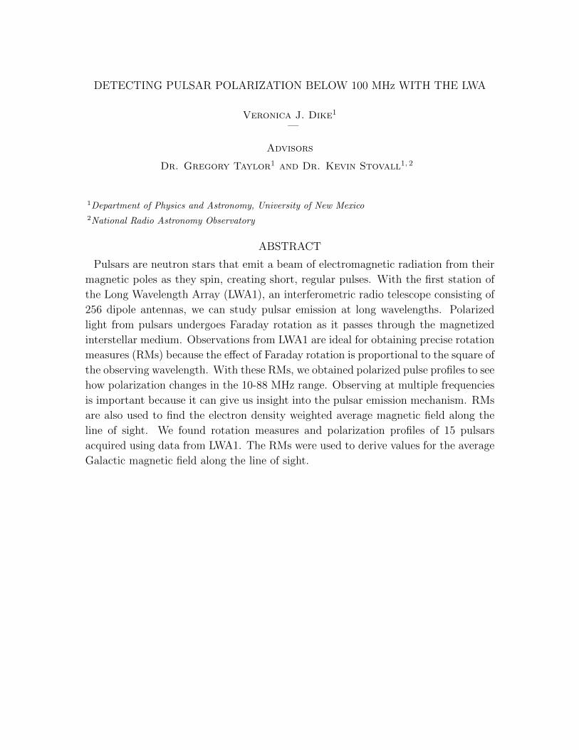
DETECTING PULSAR POLARIZATION BELOW 100 MHz WITH THE LWA

Veronica J. Dike1

—

Advisors

Dr. Gregory Taylor1 and Dr. Kevin Stovall1, 2

1Department of Physics and Astronomy, University of New Mexico2National Radio Astronomy Observatory

ABSTRACT

Pulsars are neutron stars that emit a beam of electromagnetic radiation from their

magnetic poles as they spin, creating short, regular pulses. With the first station of

the Long Wavelength Array (LWA1), an interferometric radio telescope consisting of

256 dipole antennas, we can study pulsar emission at long wavelengths. Polarized

light from pulsars undergoes Faraday rotation as it passes through the magnetized

interstellar medium. Observations from LWA1 are ideal for obtaining precise rotation

measures (RMs) because the effect of Faraday rotation is proportional to the square of

the observing wavelength. With these RMs, we obtained polarized pulse profiles to see

how polarization changes in the 10-88 MHz range. Observing at multiple frequencies

is important because it can give us insight into the pulsar emission mechanism. RMs

are also used to find the electron density weighted average magnetic field along the

line of sight. We found rotation measures and polarization profiles of 15 pulsars

acquired using data from LWA1. The RMs were used to derive values for the average

Galactic magnetic field along the line of sight.

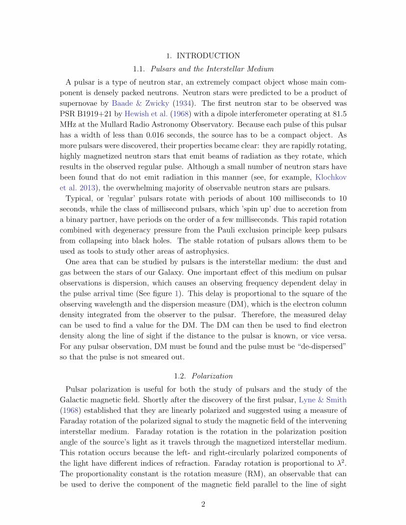
1. INTRODUCTION

1.1. Pulsars and the Interstellar Medium

A pulsar is a type of neutron star, an extremely compact object whose main com-

ponent is densely packed neutrons. Neutron stars were predicted to be a product of

supernovae by Baade & Zwicky (1934). The first neutron star to be observed was

PSR B1919+21 by Hewish et al. (1968) with a dipole interferometer operating at 81.5

MHz at the Mullard Radio Astronomy Observatory. Because each pulse of this pulsar

has a width of less than 0.016 seconds, the source has to be a compact object. As

more pulsars were discovered, their properties became clear: they are rapidly rotating,

highly magnetized neutron stars that emit beams of radiation as they rotate, which

results in the observed regular pulse. Although a small number of neutron stars have

been found that do not emit radiation in this manner (see, for example, Klochkov

et al. 2013), the overwhelming majority of observable neutron stars are pulsars.

Typical, or ’regular’ pulsars rotate with periods of about 100 milliseconds to 10

seconds, while the class of millisecond pulsars, which ’spin up’ due to accretion from

a binary partner, have periods on the order of a few milliseconds. This rapid rotation

combined with degeneracy pressure from the Pauli exclusion principle keep pulsars

from collapsing into black holes. The stable rotation of pulsars allows them to be

used as tools to study other areas of astrophysics.

One area that can be studied by pulsars is the interstellar medium: the dust and

gas between the stars of our Galaxy. One important effect of this medium on pulsar

observations is dispersion, which causes an observing frequency dependent delay in

the pulse arrival time (See figure 1). This delay is proportional to the square of the

observing wavelength and the dispersion measure (DM), which is the electron column

density integrated from the observer to the pulsar. Therefore, the measured delay

can be used to find a value for the DM. The DM can then be used to find electron

density along the line of sight if the distance to the pulsar is known, or vice versa.

For any pulsar observation, DM must be found and the pulse must be “de-dispersed”

so that the pulse is not smeared out.

1.2. Polarization

Pulsar polarization is useful for both the study of pulsars and the study of the

Galactic magnetic field. Shortly after the discovery of the first pulsar, Lyne & Smith

(1968) established that they are linearly polarized and suggested using a measure of

Faraday rotation of the polarized signal to study the magnetic field of the intervening

interstellar medium. Faraday rotation is the rotation in the polarization position

angle of the source’s light as it travels through the magnetized interstellar medium.

This rotation occurs because the left- and right-circularly polarized components of

the light have different indices of refraction. Faraday rotation is proportional to λ2.

The proportionality constant is the rotation measure (RM), an observable that can

be used to derive the component of the magnetic field parallel to the line of sight

2

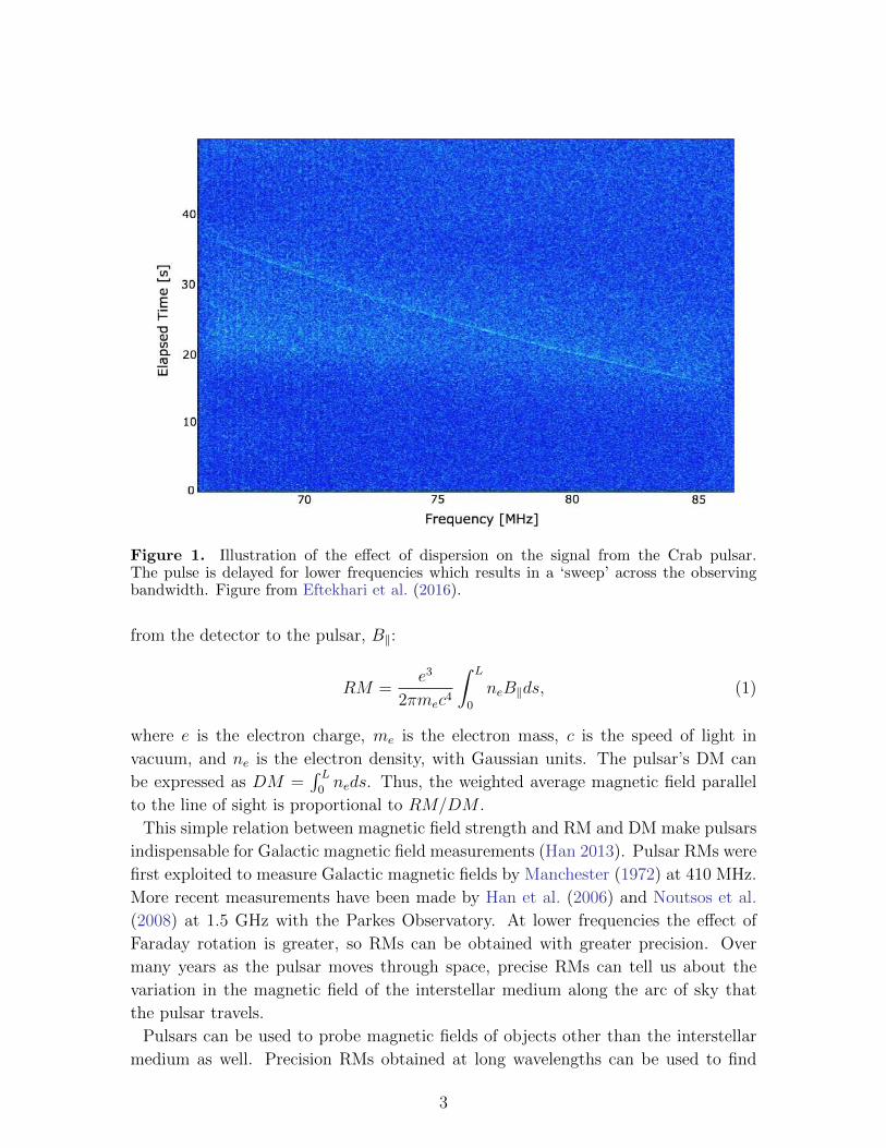
Figure 1. Illustration of the effect of dispersion on the signal from the Crab pulsar.The pulse is delayed for lower frequencies which results in a ‘sweep’ across the observingbandwidth. Figure from Eftekhari et al. (2016).

from the detector to the pulsar, B‖:

RM =e3

2πmec4

∫ L

0

neB‖ds, (1)

where e is the electron charge, me is the electron mass, c is the speed of light in

vacuum, and ne is the electron density, with Gaussian units. The pulsar’s DM can

be expressed as DM =∫ L

0neds. Thus, the weighted average magnetic field parallel

to the line of sight is proportional to RM/DM .

This simple relation between magnetic field strength and RM and DM make pulsars

indispensable for Galactic magnetic field measurements (Han 2013). Pulsar RMs were

first exploited to measure Galactic magnetic fields by Manchester (1972) at 410 MHz.

More recent measurements have been made by Han et al. (2006) and Noutsos et al.

(2008) at 1.5 GHz with the Parkes Observatory. At lower frequencies the effect of

Faraday rotation is greater, so RMs can be obtained with greater precision. Over

many years as the pulsar moves through space, precise RMs can tell us about the

variation in the magnetic field of the interstellar medium along the arc of sky that

the pulsar travels.

Pulsars can be used to probe magnetic fields of objects other than the interstellar

medium as well. Precision RMs obtained at long wavelengths can be used to find

3

the time-varying strength of the magnetic field of some object between the observer

and the pulsar, such as the Sun, as long as the effects of the ionosphere are carefully

corrected. The ionosphere is a layer of electrons above the Earth that varies on

timescales on the order of a few minutes. In spite of this challenge, Howard et al.

(2016) were able to use LWA1 to study a coronal mass ejection when PSR B0950+08

was about 5◦ from the Sun. It has also been proposed by Withers & Vogt (2017)

to use pulsars similarly for planets, although the alignment would have to be very

fortunate, and planets that emit strongly in radio such as Jupiter may overwhelm the

pulsar signal.

Another reason to measure RMs in the long wavelength regime is to study the

properties of pulsar emission. For example, it is routinely observed that linear and

circular polarization tend to decrease at shorter wavelengths. One theory for this

wavelength-dependent polarization property was put forth by von Hoensbroech et al.

(1998), assuming a magnetosphere of cold, low-density plasma: the pulsar beam

has orthogonal propagation modes that superpose due to birefringence and thus lose

polarization at higher frequencies. This theory can be tested by comparing high and

low frequency observations to see how linear and circular polarization changes (as in

Noutsos et al. 2015).

RMs can also be used to calibrate ionospheric models; see, for example, Sotomayor-

Beltran et al. (2013), in which the authors test their ionosphere modeling software

by observing four pulsars with the Low-Frequency Array (LOFAR) at different times

of day from widely-spaced stations within the array and with the higher-frequency

Westerbork Synthesis Radio Telescope. Pulsar RMs are assumed to be constant over

short timescales, so observations of a pulsar with a rotation measure known precisely

from low-frequency observations can show the diurnal variation in the ionosphere.

The multitude of reasons to examine low-frequency pulsar polarization have moti-

vated the recent studies of Johnston et al. (2008) at 243, 322 and 607 MHz with the

Giant Metrewave Radio Telescope (GMRT), Noutsos et al. (2015) at 150 MHz with

LOFAR, and Mitra et al. (2016) at 325 and 610 MHz with the GMRT. Using LWA1,

we are able to complement these studies at observing frequencies between 10 and 88

MHz.

2. OBSERVATIONS

We observed with the LWA1 station (Taylor et al. 2012), a 256-antenna dipole array

located on the Plains of San Agustin in New Mexico. The dipoles are arranged in a

pseudo-random configuration with a diameter of 100m. LWA1 is able to observe with

four independent beams simultaneously, and this beamforming capability was used

for this project. Observations were performed between July 2015 and August 2016.

Fifteen pulsars were observed with LWA1’s beamforming mode for an hour each. Two

beams were used to observe each source; each beam is split into two tunings centered

on different frequencies. This produced observations in four frequency ranges with

4

a bandwidth of 19.6 MHz. The four tunings were centered at 35.1, 49.8, 64.5, and

79.8 MHz. The raw data was coherently de-dispersed and folded using the program

DSPSR1 (van Straten & Bailes 2011). Pulsars are routinely observed with LWA1 and

de-dispersed data files are available to the public at the LWA Pulsar Data Archive2.

For more information about LWA pulsar data, see Stovall et al. (2015).

Pulsars were selected for this study if they are particularly bright in the LWA

frequency band or if there was evidence of polarization from a plot of Stokes’ pa-

rameters. Polarization components are conveniently expressed in Stokes’ parameters,

which describe the polarization of light and can be used to find the circular and lin-

ear polarization of an observation. Stokes’ parameters can also be used to find the

polarization position angle, which is the orientation of the polarization plane. Stokes’

parameters are defined as:

I = E2x + E2

y

Q = E2x − E2

y

U = 2ExEycosφ

V = 2ExEysinφ,

(2)

where each E is an electric field component and φ is the phase between the x and y

components of the field. These equations are for a linear feed, so they use the linear

electric field components. I is the total intensity, V is the circular polarization, and

linear polarization can be defined as a combination of linear components U and Q:

L =√Q2 + U2 (3)

and the polarization position angle is defined as:

ψ =1

2arctan

(U

Q

). (4)

Plots of Stokes’ Q and U over the pulse period can indicate if a pulsar is polarized.

3. METHODS

Data reduction made use of PSRCHIVE (van Straten et al. 2012), a pulsar data

analysis software package. Radio frequency interference (RFI) was removed using

a median filtering algorithm and manually through visual inspection. The rotation

measures were calculated using the method developed by Noutsos et al. (2008). The

change in total linear polarization was calculated for 512-1024 trial RMs near the value

obtained at higher observing frequency previously published in the ATNF Pulsar

Database3 (Manchester et al. 2005). The RM for each observation was found by

fitting a Gaussian peak to the plot of linear polarization vs trial RM. We corrected

1 http://dspsr.sourceforge.net/2 http://lda10g.alliance.unm.edu/PulsarArchive/3 http://www.atnf.csiro.au/people/pulsar/psrcat/

5

the linear polarization of the pulsar for the effect of the RM in order to produce

polarization profiles. The effect of Faraday rotation through the ionosphere had to

be subtracted to derive the galactic contribution to the RM. This was done using

the model developed by Sotomayor-Beltran et al. (2013). Faraday rotation through

the heliosphere was not accounted for, but this contribution is expected to be small

because our observations were made at large angles from the Sun.

4. RESULTS

4.1. Rotation Measures

We were successful in obtaining a rotation measure in at least one frequency tuning

for 15 pulsars. Table 1 lists the results as well as the period and DM of each pulsar.

Cases where RMs were unable to be found in certain frequencies are usually because

of lower sensitivity in the lowest frequency part of the band, depolarization at lower

frequencies, or RFI in that band. Note that the uncorrected RM has typical errors of

less than 0.03 rad/m2, but the ionospheric correction that follows adds considerable

uncertainty. Our results show the need for ionospheric modeling to improve so that

the accuracy achieved by low-frequency observing is not lost. There is agreement

between our results and those of Noutsos et al. (2015) and the other high-frequency

observations published in the ATNF Pulsar Database.

6

Table 1. The results of the RM fitting process for 15 pulsars. The period is taken from the ATNF Pulsar

Database and the DM is from Stovall et al. (2015). The frequency column lists the center frequency of

the beam used for each observation. Column 5 contains the RM measurement taken directly from the

observation while column 6 is the ionospheric RM at the time of observation. The rightmost column is the

observed RM with the ionospheric RM subtracted.

Pulsar Name Period DM Frequency RM Ionosphere RM Corrected RM

(s) (cm−3pc) (MHz) m−2rad) (m−2rad) (m−2rad)

B0628-28 1.2444 34.425(1)

49.8 46.67(5)

2.3(4)

44.4(4)

64.5 46.676(6) 44.4(4)

79.2 46.69(1) 44.4(4)

B0329+54 0.7145 26.779(1)64.5 −63.776(4)

2.0(2)-65.8(2)

79.2 −63.780(4) -65.8(2)

B0809+74 1.2922 5.771(2)

49.8 −13.33(1)

1.5(2)

-14.8(2)

64.5 −13.35(3) -14.8(2)

79.2 −13.36(3) -14.8(2)

B0823+26 0.5307 19.4789(2) 79.2 5.95(2) 1.3(2) 4.6(2)

B0834+06 1.2738 12.8640(4)

49.8 26.15(1)

1.6(2)

24.6(2)

64.5 26.169(6) 24.6(2)

79.2 26.129(4) 24.6(2)

B0919+06 0.4306 27.2986(5)

49.8 33.96(3)

1.3(2)

32.7(2)

64.5 33.960(4) 32.7(2)

79.2 33.90(2) 32.6(2)

B0943+10 1.0977 15.334(1)64.5 16.07(2)

3.9(2)12.2(2)

79.2 16.3(2) 12.4(3)

B0950+08 0.2531 2.96927(8)

35.1 2.210(2)

1.5(2)

0.7(2)

49.8 2.2111(4) 0.7(2)

64.5 2.209(1) 0.7(2)

79.2 2.215(3) 0.8(2)

B1133+16 1.1879 4.8480(2)

35.1 4.71(4)

1.2(2)

3.5(2)

49.8 4.710(1) 3.5(2)

64.5 4.713(3) 3.5(2)

79.2 4.719(6) 3.5(2)

B1604-00 0.4218 10.6823(1)

35.1 7.13(4)

1.4(3)

5.7(3)

49.8 7.115(3) 5.7(3)

64.5 7.10(1) 5.7(3)

Table 1 continued on next page

7

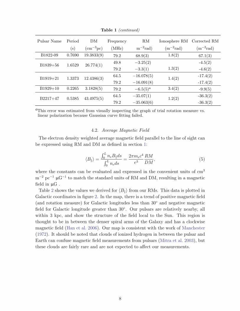
Table 1 (continued)

Pulsar Name Period DM Frequency RM Ionosphere RM Corrected RM

(s) (cm−3pc) (MHz) m−2rad) (m−2rad) (m−2rad)

B1822-09 0.7690 19.3833(9) 79.2 68.9(3) 1.8(2) 67.1(3)

B1839+56 1.6529 26.774(1)49.8 −3.25(2)

1.3(2)

-4.5(2)

79.2 −3.3(1) -4.6(2)

B1919+21 1.3373 12.4386(3)64.5 −16.078(5)

1.4(2)-17.4(2)

79.2 −16.091(8) -17.4(2)

B1929+10 0.2265 3.1828(5) 79.2 −6.5(5)a 3.4(2) -9.9(5)

B2217+47 0.5385 43.4975(5)64.5 −35.07(1)

1.2(2)-36.3(2)

79.2 −35.063(6) -36.3(2)

aThis error was estimated from visually inspecting the graph of trial rotation measure vs.linear polarization because Gaussian curve fitting failed.

4.2. Average Magnetic Field

The electron density weighted average magnetic field parallel to the line of sight can

be expressed using RM and DM as defined in section 1:

〈B‖〉 =

∫ L

0neB‖ds∫ L

0neds

=2πmec

4

e3RM

DM, (5)

where the constants can be evaluated and expressed in the convenient units of cm3

m−2 pc−1 µG−1 to match the standard units of RM and DM, resulting in a magnetic

field in µG .

Table 2 shows the values we derived for 〈B‖〉 from our RMs. This data is plotted in

Galactic coordinates in figure 2. In the map, there is a trend of positive magnetic field

(and rotation measure) for Galactic longitudes less than 30◦ and negative magnetic

field for Galactic longitude greater than 30◦. Our pulsars are relatively nearby, all

within 3 kpc, and show the structure of the field local to the Sun. This region is

thought to be in between the denser spiral arms of the Galaxy and has a clockwise

magnetic field (Han et al. 2006). Our map is consistent with the work of Manchester

(1972). It should be noted that clouds of ionized hydrogen in between the pulsar and

Earth can confuse magnetic field measurements from pulsars (Mitra et al. 2003), but

these clouds are fairly rare and are not expected to affect our measurements.

8

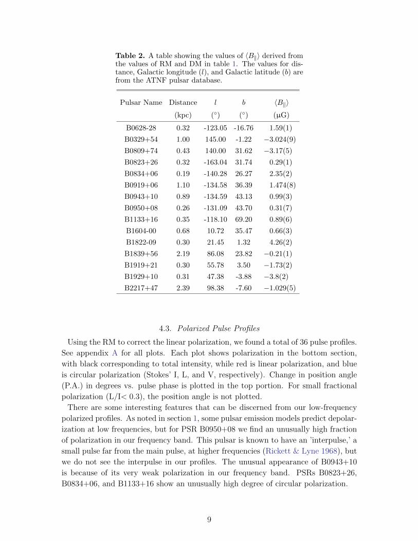
Table 2. A table showing the values of 〈B‖〉 derived fromthe values of RM and DM in table 1. The values for dis-tance, Galactic longitude (l), and Galactic latitude (b) arefrom the ATNF pulsar database.

Pulsar Name Distance l b 〈B‖〉(kpc) (◦) (◦) (µG)

B0628-28 0.32 -123.05 -16.76 1.59(1)

B0329+54 1.00 145.00 -1.22 −3.024(9)

B0809+74 0.43 140.00 31.62 −3.17(5)

B0823+26 0.32 -163.04 31.74 0.29(1)

B0834+06 0.19 -140.28 26.27 2.35(2)

B0919+06 1.10 -134.58 36.39 1.474(8)

B0943+10 0.89 -134.59 43.13 0.99(3)

B0950+08 0.26 -131.09 43.70 0.31(7)

B1133+16 0.35 -118.10 69.20 0.89(6)

B1604-00 0.68 10.72 35.47 0.66(3)

B1822-09 0.30 21.45 1.32 4.26(2)

B1839+56 2.19 86.08 23.82 −0.21(1)

B1919+21 0.30 55.78 3.50 −1.73(2)

B1929+10 0.31 47.38 -3.88 −3.8(2)

B2217+47 2.39 98.38 -7.60 −1.029(5)

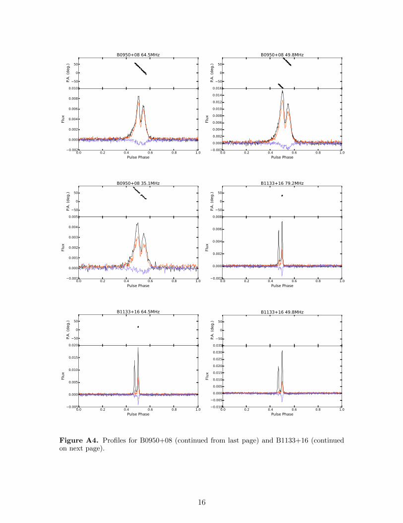
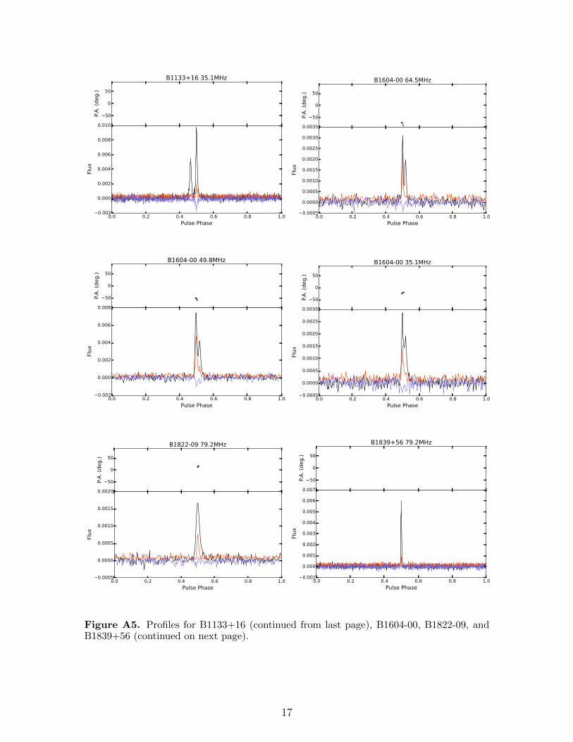
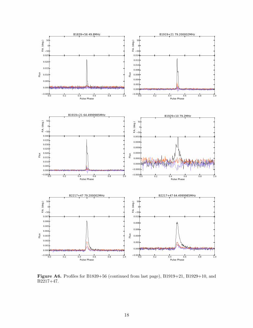
4.3. Polarized Pulse Profiles

Using the RM to correct the linear polarization, we found a total of 36 pulse profiles.

See appendix A for all plots. Each plot shows polarization in the bottom section,

with black corresponding to total intensity, while red is linear polarization, and blue

is circular polarization (Stokes’ I, L, and V, respectively). Change in position angle

(P.A.) in degrees vs. pulse phase is plotted in the top portion. For small fractional

polarization (L/I< 0.3), the position angle is not plotted.

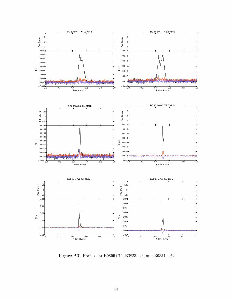
There are some interesting features that can be discerned from our low-frequency

polarized profiles. As noted in section 1, some pulsar emission models predict depolar-

ization at low frequencies, but for PSR B0950+08 we find an unusually high fraction

of polarization in our frequency band. This pulsar is known to have an ’interpulse,’ a

small pulse far from the main pulse, at higher frequencies (Rickett & Lyne 1968), but

we do not see the interpulse in our profiles. The unusual appearance of B0943+10

is because of its very weak polarization in our frequency band. PSRs B0823+26,

B0834+06, and B1133+16 show an unusually high degree of circular polarization.

9

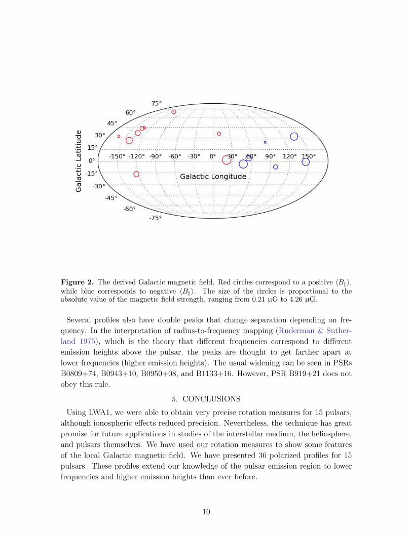
Figure 2. The derived Galactic magnetic field. Red circles correspond to a positive 〈B‖〉,while blue corresponds to negative 〈B‖〉. The size of the circles is proportional to theabsolute value of the magnetic field strength, ranging from 0.21 µG to 4.26 µG.

Several profiles also have double peaks that change separation depending on fre-

quency. In the interpretation of radius-to-frequency mapping (Ruderman & Suther-

land 1975), which is the theory that different frequencies correspond to different

emission heights above the pulsar, the peaks are thought to get farther apart at

lower frequencies (higher emission heights). The usual widening can be seen in PSRs

B0809+74, B0943+10, B0950+08, and B1133+16. However, PSR B919+21 does not

obey this rule.

5. CONCLUSIONS

Using LWA1, we were able to obtain very precise rotation measures for 15 pulsars,

although ionospheric effects reduced precision. Nevertheless, the technique has great

promise for future applications in studies of the interstellar medium, the heliosphere,

and pulsars themselves. We have used our rotation measures to show some features

of the local Galactic magnetic field. We have presented 36 polarized profiles for 15

pulsars. These profiles extend our knowledge of the pulsar emission region to lower

frequencies and higher emission heights than ever before.

10

REFERENCES

Baade, W., & Zwicky, F. 1934,Proceedings of the National Academyof Science, 20, 259

Eftekhari, T., Stovall, K., Dowell, J.,Schinzel, F. K., & Taylor, G. B. 2016,ApJ, 829, 62

Han, J. 2013, in IAU Symposium, Vol.291, Neutron Stars and Pulsars:Challenges and Opportunities after 80years, ed. J. van Leeuwen, 223–228

Han, J. L., Manchester, R. N., Lyne,A. G., Qiao, G. J., & van Straten, W.2006, ApJ, 642, 868

Hewish, A., Bell, S. J., Pilkington,J. D. H., Scott, P. F., & Collins, R. A.1968, Nature, 217, 709

Howard, T. A., Stovall, K., Dowell, J.,Taylor, G. B., & White, S. M. 2016,ApJ, 831, 208

Johnston, S., Karastergiou, A., Mitra, D.,& Gupta, Y. 2008, MNRAS, 388, 261

Klochkov, D., Puhlhofer, G., Suleimanov,V., et al. 2013, A&A, 556, A41

Lyne, A. G., & Smith, F. G. 1968,Nature, 218, 124

Manchester, R. N. 1972, ApJ, 172, 43Manchester, R. N., Hobbs, G. B., Teoh,

A., & Hobbs, M. 2005, AJ, 129, 1993Mitra, D., Basu, R., Maciesiak, K., et al.

2016, ApJ, 833, 28Mitra, D., Wielebinski, R., Kramer, M., &

Jessner, A. 2003, A&A, 398, 993

Noutsos, A., Johnston, S., Kramer, M., &

Karastergiou, A. 2008, MNRAS, 386,

1881

Noutsos, A., Sobey, C., Kondratiev, V. I.,

et al. 2015, A&A, 576, A62

Rickett, B. J., & Lyne, A. G. 1968,

Nature, 218, 934

Ruderman, M. A., & Sutherland, P. G.

1975, ApJ, 196, 51

Sotomayor-Beltran, C., Sobey, C.,

Hessels, J. W. T., et al. 2013, A&A,

552, A58

Stovall, K., Ray, P. S., Blythe, J., et al.

2015, ApJ, 808, 156

Taylor, G. B., Ellingson, S. W., Kassim,

N. E., et al. 2012, Journal of

Astronomical Instrumentation, 1,

1250004

van Straten, W., & Bailes, M. 2011,

PASA, 28, 1

van Straten, W., Demorest, P., &

Oslowski, S. 2012, Astronomical

Research and Technology, 9, 237

von Hoensbroech, A., Lesch, H., & Kunzl,

T. 1998, A&A, 336, 209

Withers, P., & Vogt, M. F. 2017, ApJ,

836, 114

Typeset using LATEX modern style in AASTeX61

APPENDIX

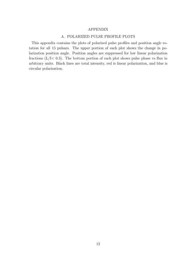
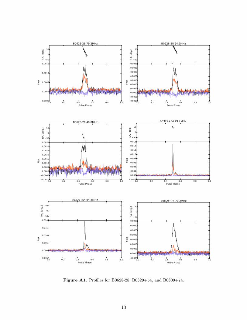
A. POLARIZED PULSE PROFILE PLOTS

This appendix contains the plots of polarized pulse profiles and position angle ro-

tation for all 15 pulsars. The upper portion of each plot shows the change in po-

larization position angle. Position angles are suppressed for low linear polarization

fractions (L/I< 0.3). The bottom portion of each plot shows pulse phase vs flux in

arbitrary units. Black lines are total intensity, red is linear polarization, and blue is

circular polarization.

12

−50

0

50

P.A. (de

g.)

B0628-28 79.2MHz

0.0 0.2 0.4 0.6 0.8 1.0Pulse Phase

−0.0005

0.0000

0.0005

0.0010

0.0015

Flux

−50

0

50

P.A. (de

g.)

B0628-28 64.5MHz

0.0 0.2 0.4 0.6 0.8 1.0Pulse Phase

−0.0010

−0.0005

0.0000

0.0005

0.0010

0.0015

0.0020

0.0025

0.0030

0.0035

Flux

−50

0

50

P.A. (de

g.)

B0628-28 49.8MHz

0.0 0.2 0.4 0.6 0.8 1.0Pulse Phase

−0.0010

−0.0005

0.0000

0.0005

0.0010

0.0015

0.0020

0.0025

0.0030

0.0035

Flux

−50

0

50P.A

. (de

g.)

B0329+54 79.2MHz

0.0 0.2 0.4 0.6 0.8 1.0Pulse Phase

−0.002

0.000

0.002

0.004

0.006

0.008

0.010

0.012

0.014

0.016

Flux

−50

0

50

P.A. (de

g.)

B0329+54 64.5MHz

0.0 0.2 0.4 0.6 0.8 1.0Pulse Phase

−0.005

0.000

0.005

0.010

0.015

0.020

Flux

−50

0

50

P.A. (de

g.)

B0809+74 79.2MHz

0.0 0.2 0.4 0.6 0.8 1.0Pulse Phase

−0.0005

0.0000

0.0005

0.0010

0.0015

0.0020

0.0025

0.0030

0.0035

Flux

Figure A1. Profiles for B0628-28, B0329+54, and B0809+74.

13

−50

0

50P.A

. (de

g.)

B0809+74 64.5MHz

0.0 0.2 0.4 0.6 0.8 1.0Pulse Phase

−0.001

0.000

0.001

0.002

0.003

0.004

0.005

0.006

0.007

0.008

Flux

−50

0

50

P.A. (de

g.)

B0809+74 49.8MHz

0.0 0.2 0.4 0.6 0.8 1.0Pulse Phase

−0.002

0.000

0.002

0.004

0.006

0.008

0.010

0.012

Flux

−50

0

50

P.A. (de

g.)

B0823+26 79.2MHz

0.0 0.2 0.4 0.6 0.8 1.0Pulse Phase

−0.0005

0.0000

0.0005

0.0010

0.0015

0.0020

0.0025

0.0030

0.0035

0.0040

Flux

−50

0

50

P.A. (de

g.)

B0834+06 79.2MHz

0.0 0.2 0.4 0.6 0.8 1.0Pulse Phase

−0.002

0.000

0.002

0.004

0.006

0.008

0.010

0.012

0.014

Flux

−50

0

50

P.A. (de

g.)

B0834+06 64.5MHz

0.0 0.2 0.4 0.6 0.8 1.0Pulse Phase

−0.01

0.00

0.01

0.02

0.03

0.04

Flux

−50

0

50

P.A. (de

g.)

B0834+06 49.8MHz

0.0 0.2 0.4 0.6 0.8 1.0Pulse Phase

−0.01

0.00

0.01

0.02

0.03

0.04

0.05

0.06

0.07

Flux

Figure A2. Profiles for B0809+74, B0823+26, and B0834+06.

14

−50

0

50P.A

. (de

g.)

B0919+06 79.2MHz

0.0 0.2 0.4 0.6 0.8 1.0Pulse Phase

−0.0005

0.0000

0.0005

0.0010

0.0015

0.0020

0.0025

Flux

−50

0

50

P.A. (de

g.)

B0919+06 64.5MHz

0.0 0.2 0.4 0.6 0.8 1.0Pulse Phase

−0.001

0.000

0.001

0.002

0.003

0.004

0.005

0.006

0.007

Flux

−50

0

50

P.A. (de

g.)

B0919+06 49.8MHz

0.0 0.2 0.4 0.6 0.8 1.0Pulse Phase

−0.002

0.000

0.002

0.004

0.006

0.008

0.010

0.012

0.014

Flux

−50

0

50

P.A. (de

g.)

B0943+10 79.2MHz

0.0 0.2 0.4 0.6 0.8 1.0Pulse Phase

−0.0002

0.0000

0.0002

0.0004

0.0006

0.0008

0.0010

0.0012

Flux

−50

0

50

P.A. (de

g.)

B0943+10 64.5MHz

0.0 0.2 0.4 0.6 0.8 1.0Pulse Phase

−0.001

0.000

0.001

0.002

0.003

0.004

0.005

0.006

Flux

−50

0

50

P.A. (de

g.)

B0950+08 79.2MHz

0.0 0.2 0.4 0.6 0.8 1.0Pulse Phase

−0.0010

−0.0005

0.0000

0.0005

0.0010

0.0015

0.0020

0.0025

0.0030

0.0035

Flux

Figure A3. Profiles for B0919+06, B0943+10, and B0950+08 (continued on next page).

15

−50

0

50P.A

. (de

g.)

B0950+08 64.5MHz

0.0 0.2 0.4 0.6 0.8 1.0Pulse Phase

−0.002

0.000

0.002

0.004

0.006

0.008

0.010

Flux

−50

0

50

P.A. (de

g.)

B0950+08 49.8MHz

0.0 0.2 0.4 0.6 0.8 1.0Pulse Phase

−0.002

0.000

0.002

0.004

0.006

0.008

0.010

0.012

0.014

0.016

Flux

−50

0

50

P.A. (de

g.)

B0950+08 35.1MHz

0.0 0.2 0.4 0.6 0.8 1.0Pulse Phase

−0.001

0.000

0.001

0.002

0.003

0.004

0.005

Flux

−50

0

50

P.A. (de

g.)

B1133+16 79.2MHz

0.0 0.2 0.4 0.6 0.8 1.0Pulse Phase

−0.002

0.000

0.002

0.004

0.006

0.008

Flux

−50

0

50

P.A. (de

g.)

B1133+16 64.5MHz

0.0 0.2 0.4 0.6 0.8 1.0Pulse Phase

−0.005

0.000

0.005

0.010

0.015

0.020

Flux

−50

0

50

P.A. (de

g.)

B1133+16 49.8MHz

0.0 0.2 0.4 0.6 0.8 1.0Pulse Phase

−0.010

−0.005

0.000

0.005

0.010

0.015

0.020

0.025

0.030

0.035

Flux

Figure A4. Profiles for B0950+08 (continued from last page) and B1133+16 (continuedon next page).

16

−50

0

50P.A

. (de

g.)

B1133+16 35.1MHz

0.0 0.2 0.4 0.6 0.8 1.0Pulse Phase

−0.002

0.000

0.002

0.004

0.006

0.008

0.010

Flux

−50

0

50

P.A. (de

g.)

B1604-00 64.5MHz

0.0 0.2 0.4 0.6 0.8 1.0Pulse Phase

−0.0005

0.0000

0.0005

0.0010

0.0015

0.0020

0.0025

0.0030

0.0035

Flux

−50

0

50

P.A. (de

g.)

B1604-00 49.8MHz

0.0 0.2 0.4 0.6 0.8 1.0Pulse Phase

−0.002

0.000

0.002

0.004

0.006

0.008

Flux

−50

0

50

P.A. (de

g.)

B1604-00 35.1MHz

0.0 0.2 0.4 0.6 0.8 1.0Pulse Phase

−0.0005

0.0000

0.0005

0.0010

0.0015

0.0020

0.0025

0.0030

Flux

−50

0

50

P.A. (de

g.)

B1822-09 79.2MHz

0.0 0.2 0.4 0.6 0.8 1.0Pulse Phase

−0.0005

0.0000

0.0005

0.0010

0.0015

0.0020

Flux

−50

0

50

P.A. (de

g.)

B1839+56 79.2MHz

0.0 0.2 0.4 0.6 0.8 1.0Pulse Phase

−0.001

0.000

0.001

0.002

0.003

0.004

0.005

0.006

0.007

Flux

Figure A5. Profiles for B1133+16 (continued from last page), B1604-00, B1822-09, andB1839+56 (continued on next page).

17

−50

0

50P.A

. (de

g.)

B1839+56 49.8MHz

0.0 0.2 0.4 0.6 0.8 1.0Pulse Phase

−0.005

0.000

0.005

0.010

0.015

0.020

0.025

Flux

−50

0

50

P.A. (de

g.)

B1919+21 79.200002MHz

0.0 0.2 0.4 0.6 0.8 1.0Pulse Phase

−0.002

0.000

0.002

0.004

0.006

0.008

0.010

0.012

0.014

Flux

−50

0

50

P.A. (de

g.)

B1919+21 64.4999985MHz

0.0 0.2 0.4 0.6 0.8 1.0Pulse Phase

−0.005

0.000

0.005

0.010

0.015

0.020

0.025

0.030

0.035

0.040

Flux

−50

0

50

P.A. (de

g.)

B1929+10 79.2MHz

0.0 0.2 0.4 0.6 0.8 1.0Pulse Phase

−0.0004

−0.0002

0.0000

0.0002

0.0004

0.0006

0.0008

0.0010

Flux

−50

0

50

P.A. (de

g.)

B2217+47 79.200002MHz

0.0 0.2 0.4 0.6 0.8 1.0Pulse Phase

−0.001

0.000

0.001

0.002

0.003

0.004

0.005

0.006

0.007

Flux

−50

0

50

P.A. (de

g.)

B2217+47 64.4999985MHz

0.0 0.2 0.4 0.6 0.8 1.0Pulse Phase

−0.002

0.000

0.002

0.004

0.006

0.008

0.010

Flux

Figure A6. Profiles for B1839+56 (continued from last page), B1919+21, B1929+10, andB2217+47.

18