Verification of Welding Power Input in Two-Dimensional

Verification of Welding Power

Input in Two-Dimensional Welding Simulation

V&V2012-6181

Session: 8-2 Validation Methods for Materials Engineering: Part 2

ASME Verification and Validation Symposium (V&V2012) Planet Hollywood Resort & Casino, Las Vegas

May 3, 2012

(Revised May 18, 2012)

Dave Dewees, P.E.

The Equity Engineering Group, Inc.

2

Introduction

• The fundamental input to the heat transfer model is the welding arc power, typically represented as

– an assigned triple Gaussian function (Goldak double ellipsoid model)

– or more simply, as a uniform temperature

• Methods for verification relative to the intended welding power are presented for the special case of 2D analysis, and results for the two methods are compared

DFLUX Uniform Temperature Assignment

3

Heat Input Methods

• Simplest approach for representing heat from welding torch in thermal FEA of welding is to assign temperature of melt to added material region for pass

• This method is widely used and documented

• There are two potential issues with uniform temperature assignment

– Re-melt/tie-in is not usually considered

– Actual heat input is often greater than uniform temperature assumption gives

4

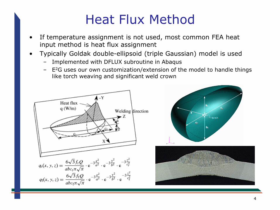
Heat Flux Method

• If temperature assignment is not used, most common FEA heat input method is heat flux assignment

• Typically Goldak double-ellipsoid (triple Gaussian) model is used

– Implemented with DFLUX subroutine in Abaqus

– E2G uses our own customization/extension of the model to handle things like torch weaving and significant weld crown

5

Heat Flux Method

• The heat flux method is attractive because it directly incorporates the weld power

• The Goldak model defines a spatially varying power density function (power per unit volume)

– When integrated over the application region (the 3D composite ellipsoid), the welding power (in Watts or btu/s) should be returned!

– See Goldak 1985 and Lindgren 2008 for illustration of the formulation and integration

• Modern math tools make this a very easy check, even over the actual 3D ellipsoidal volume:

6

Heat Flux Method

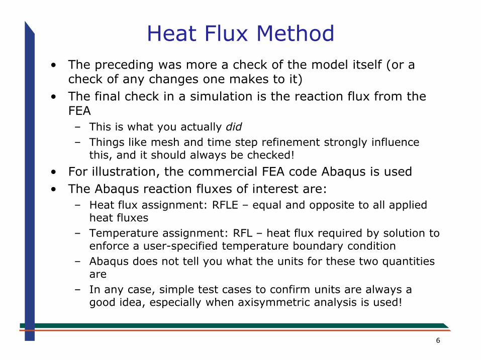
• The preceding was more a check of the model itself (or a check of any changes one makes to it)

• The final check in a simulation is the reaction flux from the FEA

– This is what you actually did

– Things like mesh and time step refinement strongly influence this, and it should always be checked!

• For illustration, the commercial FEA code Abaqus is used

• The Abaqus reaction fluxes of interest are:

– Heat flux assignment: RFLE – equal and opposite to all applied heat fluxes

– Temperature assignment: RFL – heat flux required by solution to enforce a user-specified temperature boundary condition

– Abaqus does not tell you what the units for these two quantities are

– In any case, simple test cases to confirm units are always a good idea, especially when axisymmetric analysis is used!

7

RFLE Units

• Simple steady state test problem with known solution to confirm units

• Cylindrical problem to give enough complexity to test all uncertainties:

.applied leftq

.applied rightq

.applied leftq .applied rightq

8

RFL Units

• Units of power/circumference were required for the axisymmetric surface flux input, and output was just in units of power (i.e. RFLE → btu/s)

• The same test case is used to test the units for RFL, except that the 100 degree temperature gradient is imposed at the boundaries

• So the units for RFL are the same as RFLE (power: Watts or btu/s)

temperature boundary condition:

200°F

temperature boundary condition:

100°F

9

Reaction Flux Usage

• This exercise can be extended to show that when reaction fluxes are totaled/summed over the entire model, the result is the total power input for a given time step

• When multiplied by the corresponding time step (for step application of boundary conditions), the actual modeled energy is returned

• This is perhaps the best comparison measure since all that’s needed is: [(travel distance)/(travel speed)](net weld power) = total energy

• Prior to demonstrating verification of heat input for temperature and heat flux assignment, the chosen test case is described

10

Test Case

• British Energy 316 stainless steel 7 pass pipe welds

• Discussed and validated against extensively in literature, and through the course of recent PVRV WRS JIP

11

Test Case

• Detailed info. is available in ASME JPVT (Dong 2001); good candidate to compare DFLUX approach

• PVP analysis lumped one pass and modeled as a 6 pass weld

• For this analysis all 7 passes are modeled

12

Test Case

• Experimental data from 2 mockups

13

Finite Element Analysis

• Uncoupled, sequential thermal-stress analysis

• Only thermal analysis is changed – temperature assignment and heat flux assignment used to represent welding power input

• Same FE mesh, material properties used in all cases, and stress runs are identical (only difference is thermal results file read)

• Linear, full integration elements used (2439 nodes, 2216 elements)

14

Thermal Analysis Steps

• Initial Conditions:

– Assigned Temperature: weld = 2732F base = 70F

– Assigned Heat Flux: weld = 70F base = 70F

• Boundary Conditions:

– Preheat temperature = 70F

– h = 1.0 btu/hr-ft2-F, T = 70F (interpass temperature)

– Birthing steps for assigned temperature: 2732F for 1 to 3 seconds

• Analysis steps:

1st Pass All Subsequent Passes

1 Remove all but 1st pass from model

1 Add current pass to model

2 Step 1st pass base metal boundary nodes to 2732F or assign heat flux

2 Step pass base metal boundary nodes to 2732F or assign heat flux

3 Remove boundary node BC or heat flux and let model cool for 1200 sec

3 Remove boundary node BC or heat flux and let model cool for 1200 sec

4 Set temperatures to interpass (70F)

4 Set temperatures to interpass (70F)

15

Stress Analysis Steps

• Initial Conditions:

– weld = 2192F base = 70F

• Thermal Expansion:

– Tref.a.weld = 2192F Tref.a.base = 70F

• Boundary conditions: symmetry (rollers) at weld half-plane

• Large displacement analysis

• Analysis steps:

1st Pass All Subsequent Passes

1 Remove all but 1st pass from model

1 Add current pass to model

2-4 Read temperatures from thermal analysis

2-4 Read temperatures from thermal analysis

16

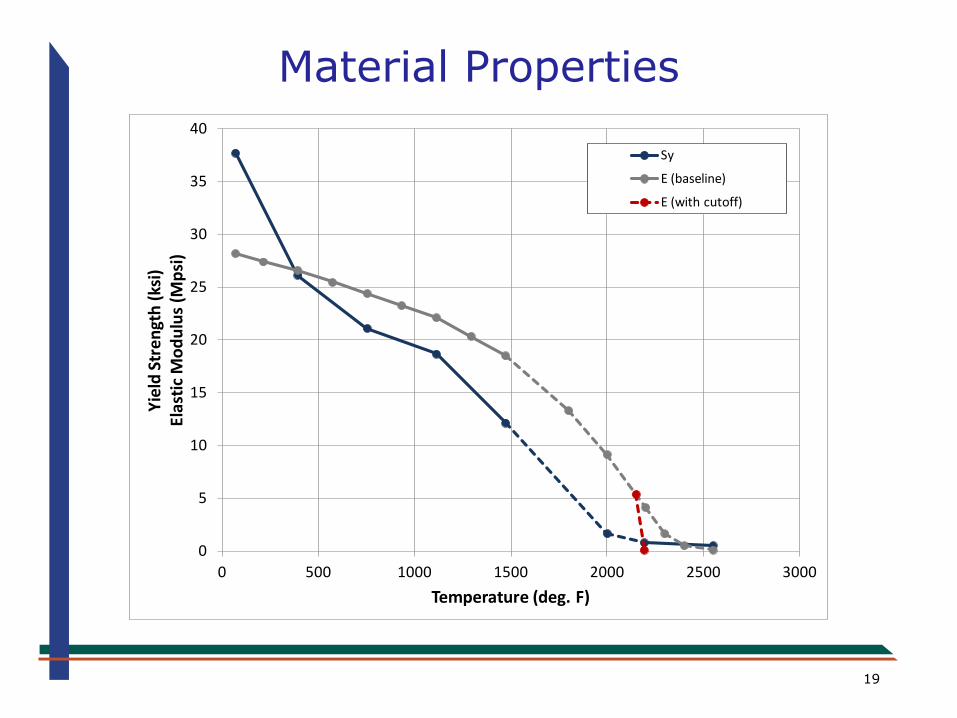
Methodology • A cutoff temperature of ≈0.8Tm(K) is used

– Above 0.8Tm high temperature phenomena (such as rapid stress relaxation and dynamic recrystallization) dominate the material response and stresses that would be modeled in FEA at these temperatures would have no physical meaning

– Temperature history is filtered with simple subroutine

– Cutoff temperature here is taken as annealing temperature: 2192F

• Weld metal is defined as stress free at the cutoff temperature (shrinks as it cools) – expansion coefficient recalculated for new reference temperature

– Large displacement analysis is used

– All elements are active for entire analysis, but since they are at melt, they float along

– This allows them to be completely annealed (elastic and plastic strain) by updating pass reference configuration (using *Model Change, add=strain free) right before the pass is to become active

Stress free at cutoff temperature

17

Methodology

• Large deflection analysis avoids typical element birthing severe mesh distortion and convergence problems

• Seam weld example shown below (seam weld simulations are particularly sensitive):

18

Material Properties

• Properties and results are from JIP and E2G property survey

0.100

0.110

0.120

0.130

0.140

0.150

0.160

5

7

9

11

13

15

17

19

0 200 400 600 800 1000 1200 1400 1600 1800

Spe

cifi

c H

eat

, cp

(btu

/lb

-°F)

The

rmal

Co

nd

uct

ivit

y, k

(btu

/hr-

ft-°

F)

Co

eff

icie

nt o

f Lin

ear

Th

erm

al E

xpan

sio

n/1

0-6

,a(i

n./

in-°

F)

Temperature (deg. F)

k

CTE

cp

r = 0.29 (constant)

Tsolidus = 2550°FTliquidus = 2650°Flatent heat = 112 btu/lb

19

Material Properties

0

5

10

15

20

25

30

35

40

0 500 1000 1500 2000 2500 3000

Yie

ld S

tren

gth

(ks

i)El

asti

c M

od

ulu

s (M

psi

)

Temperature (deg. F)

Sy

E (baseline)

E (with cutoff)

20

Material Properties

0

10000

20000

30000

40000

50000

60000

70000

80000

90000

0 0.02 0.04 0.06 0.08 0.1

Stre

ss (

psi

)

Plastic Strain

20C/68F

200C/392F

400C/752F

600C/1112F

800C/1472F

2000F

1200C/2192F

21

Assigned Heat Flux Analysis

• Thermal analysis uses Goldak double ellipsoidal power density-based model for all passes

• Since no cross-section is available, it’s assumed the added material shape is representative and re-melting follows the general shape of the added material

22

Assigned Heat Flux Analysis

• Although the heat flux assignment coding is not difficult conceptually, it is somewhat involved

• One way to verify that the subroutine is behaving as intended is to output the calculated power density at each material point for a time step and plot them:

This is really just a snapshot; a more comprehensive verification is described on the following slides . . .

23

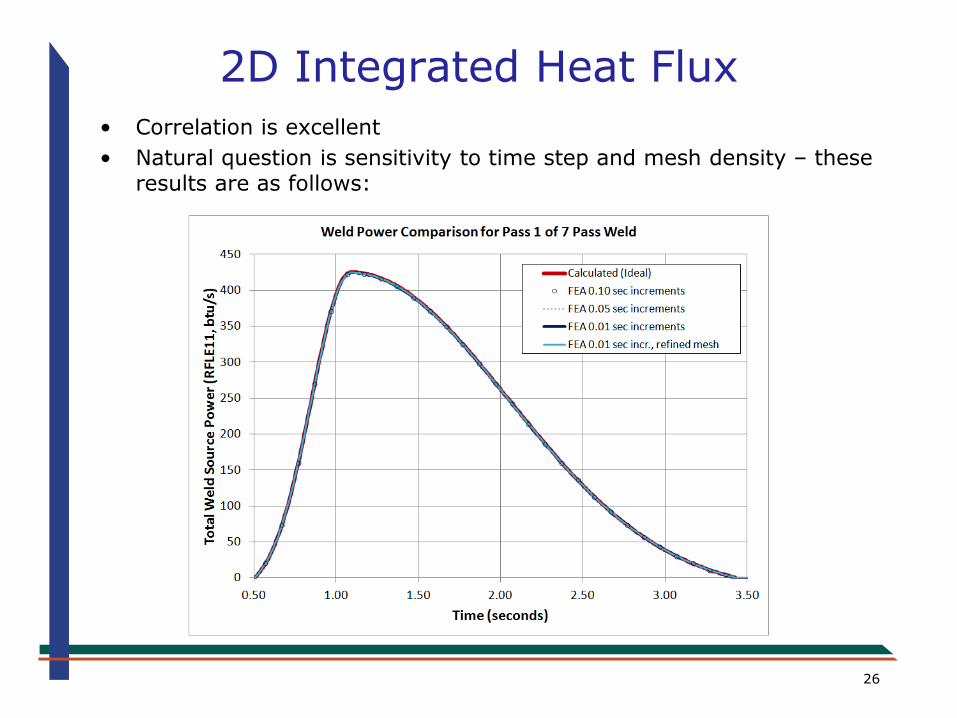
2D Integrated Heat Flux

• Heat flux is assigned through the user subroutine DFLUX

– Same subroutine coding is used for 2D or 3D analysis

– In 2D the source just moves through the single plane of the analysis

+ In the actual (3D) case, every plane of the weld will see every cross-section of the power density heat input (within the constraints of mesh and time step refinement) but at different times

+ In 2D, every cross section simply sees each cross-section of the power density heat source at the same time

• The summed value of power on the cross section for a given power density cross-section is a bit unintuitive, but can certainly be defined

24


• The only input to this function is the axial position of interest:

– Relative to the current position of the heat source center

– This can be returned from the subroutine or calculated based on known time and travel speed

– This function can be evaluated at every increment/time step to determine what the ideal 2D heat input is

• The units of the above function are power/circumference – multiply by 2pr to get overall power to compare to RFLE

25


• Result for pass 1 of the 7 pass weld is shown below:

0

50

100

150

200

250

300

350

400

450

0.50 1.00 1.50 2.00 2.50 3.00 3.50

Tota

l We

ld S

ou

rce

Po

we

r (R

FLE1

1, b

tu/s

)

Time (seconds)

Weld Power Comparison for Pass 1 of 7 Pass Weld

Calculated (Ideal)

FEA (Totaled RFLE from .dat file)

26


• Correlation is excellent

• Natural question is sensitivity to time step and mesh density – these results are as follows:

27


• RFLE values for the different time increments all fall on the same curve – no time increment sensitivity

• The importance of the time increment is related to accuracy of the weld energy, which is taken as constant over each increment

• The mesh size does not appear to be a variable either

• However:

– In this case, what’s actually demonstrated is mesh convergence

– RFLE accuracy IS pre-determined by the fineness of the mesh - flux values are only calculated at the discrete integration points and taken as constant over the entire area associated with the points

28

Total Energy

• Multiplying each time increment power (summed reaction flux) value by the time increment and summing gives the total FEA energy input for the pass

• As mentioned previously, this result should equal the known welding inputs:

• The results are:

tan

ideal

travel dis ceQ E I

travel speed

pass R_avg I E eta v (ipm) BTU/s BTU/in_ideal* BTU_ideal a (0.1s) b (0.05s) c (0.01s)

1 15.5650 85 22.5 0.86 7.68 1.559 6.090 595.6 594.5 594.2 594.3

2 15.4636 121 23 0.90 6.21 2.374 11.47 1114 1120 1119 1119

3 15.3801 156 22.4 0.38 5.95 1.259 10.47 1012 995.7 993.5 993.2

4 15.7118 300 28 0.41 15 3.264 6.528 644.4 645.3 645.7 645.5

5 15.8601 421 30 0.88 14 10.534 22.57 2249 2253 2250 2250

6 16.0127 421 30 0.52 14 6.225 18.01 1812 1812 1811 1809

7 16.1133 440 30 0.75 14 9.383 26.14 2646 2647 2650 2647

*Energy input divided by two due to half-symmetry FEA model

29

Total Energy

• The maximum difference from ideal for any pass in this case is 1.9%

• All other differences are less than 0.5% (for all time steps and both meshes)

• This demonstrates that the welding power is accurately reproduced from the 2D analysis

• This also demonstrates that there is a direct and obvious relationship between the welding power and 2D FEA, although it has been suggested in the literature that this is not the case

• These results are for heat flux assignment – temperature assignment is discussed next

30

Assigned Temperature Analysis

• In the assigned temperature, the weld is defined at high temperature (here 2732°F) initially, but is removed from the

analysis domain prior to solution

• Element sets corresponding to each pass are brought in one (pass) at a time

– The model nodes adjacent to the pass elements about to birthed are step-changed to the weld temperature and held for a “pre-heating” time

– Pre-heating times of up to 3 seconds are common

– Pre-heat step is sometimes implemented as a ramp (easier convergence), with a correspondingly lower equivalent heat input

– After the preheat step (with weld elements present at the weld temperature) all temperature boundary conditions are removed and the transient conduction problem is solved until the weld has cooled back near interpass or room temperature

31


• The length of the pre-heat step is intended to mimic penetration into adjacent existing material

• By definition though, no adjacent nodes will ever reach the assigned boundary node temperature

• However, the longer the pre-heat step is held, the greater the equivalent heat input

• To help overcome this, the weld temperature is assigned something higher than melt (i.e. 2732°F vs. 2650°F assumed liquidus)

(From Lindgren 2008)

32


• Note that temperature assignment does not have to be uniform

• In fact, the parabolic temperature assignment discussed in Goldak 2005 accounts for re-melting and tie-in and gives results nearly identical to the double ellipsoidal power density approach in this author’s experience

• said another way, the double ellipsoidal power density approach gives a temperature profile that varies parabolically on any line from the single maximum at the source/torch center to the melt temperature boundary

33

Thermal Results Comparison

• 3 sec. preheat time with excess temperature is chosen because it seems to give closest match to heat flux analysis

• 1 sec. preheat would not be an uncommon time selection, but as can be seen, gives substantially less thermal penetration

DFLUX 3 sec. 1 sec.

34


0

1000

2000

3000

4000

5000

6000

0 500 1000 1500 2000 2500 3000 3500 4000

Tem

pe

ratu

re (d

eg.

F)

Time (seconds)

Temperature History Comparison in Pass 5

Assigned Heat Flux

Assigned Temperature (3 sec. preheat)

35


• Results from another study show greater differences can exist when care is not taken

• Results are typically many hundreds of degrees different:

400

600

800

1000

1200

1400

1600

1800

2000

2200

2400

0 50000 100000 150000 200000 250000

Tem

per

atu

re (d

eg.

F)

Time (seconds)

Uniform Temperature Assignment (heat transfer analysis)

DFLUX (heat transfer analysis)

DFLUX (filtered results for stress analysis)

36

Required Heat Flux

• Just as the actual reaction flux can be tracked and totaled in the assigned heat flux analysis, RFL can be summed for assigned temperature analysis:

0

50

100

150

200

250

300

350

400

450

0.50 1.00 1.50 2.00 2.50 3.00 3.50

Tota

l We

ld S

ou

rce

Po

we

r (R

FLE

and

RFL

, btu

/s)

Time (seconds)

Weld Power Comparison for Pass 1 of 7 Pass Weld

Calculated (Ideal)

FEA 0.10 sec increments



FEA 0.01 sec incr., refined mesh

Assigned Temperature - 1s preheat

Assigned Temperature - 3s preheat

37

Required Heat Flux

• Note that the shape of the power history for the assigned temperature reflects the shape of the step application of the boundary condition (but will always be different than the double ellipsoid approaches)

• Before comparing total required powers with the flux approach:

– need to add the energy required to bring material to the assumed FEA started condition (2732°F):

– Average specific heat, cp (0.15 btu/lb-F) used with density, r (0.29 lb/in3) and latent heat, hf (112.2 btu/lb)

. . .sec2 2732 70pass centroid pass cross tion p fEnergy R A c hp r

Pass R

(in) Area (in2)

Volume (in3)

Mass (lb)

Energy (btu)

1 15.565 0.0072 0.705 0.204 105

2 15.464 0.0134 1.300 0.377 193

3 15.380 0.0169 1.632 0.473 242

4 15.712 0.0081 0.798 0.231 118

5 15.860 0.0350 3.488 1.011 517

6 16.013 0.0329 3.314 0.961 492

7 16.113 0.0438 4.435 1.286 658

38

Required Heat Flux

• The total required powers are then as follows (all values in BTU):

Pass Intended

Qideal

Assigned Heat Flux

Assigned Temperature

1 sec. preheat

Assigned Temperature

3 sec. preheat

1 595.6 594.5 362.8 (-39.1%)

595.9 (0%)

2 1114.3 1119.9 557.5 (-50.0%)

702.9 (-36.9%)

3 1012.0 995.7 626.9 (-38.1%)

768.3 (-24.1%)

4 644.4 645.3 418.8 (-35.0%)

710.7 (+10.3%)

5 2249.4 2253.3 1016 (-54.8%)

1435 (-36.2%)

6 1811.9 1811.8 1003 (-44.6%)

1404 (-22.5%)

7 2646.3 2646.7 1351 (-48.9%)

1866 (-29.5%)

39

Required Heat Flux

• While differences of 0.5% from ideal/intended were typical for the assigned heat flux approach, typical assigned temperature differences are 20-40%

• If the end goal was thermal analysis alone, or perhaps microstructure analysis, these differences are significant

• Stress analysis is assumed to be the end goal here, or more specifically flaw evaluation

• Stress results are compared on the following slides

• Note that linearized stress (through-wall crack opening membrane + bending, or “M+B”) would be the typical input to a flaw assessment

40

Hoop Stress Comparison

Results in MPa

JIP Phase 1 Report

Temperature Assignment

Heat Flux Assignment

41

Axial Stress Comparison

JIP Phase 1 Report

Temperature Assignment

Heat Flux Assignment

Results in MPa

42

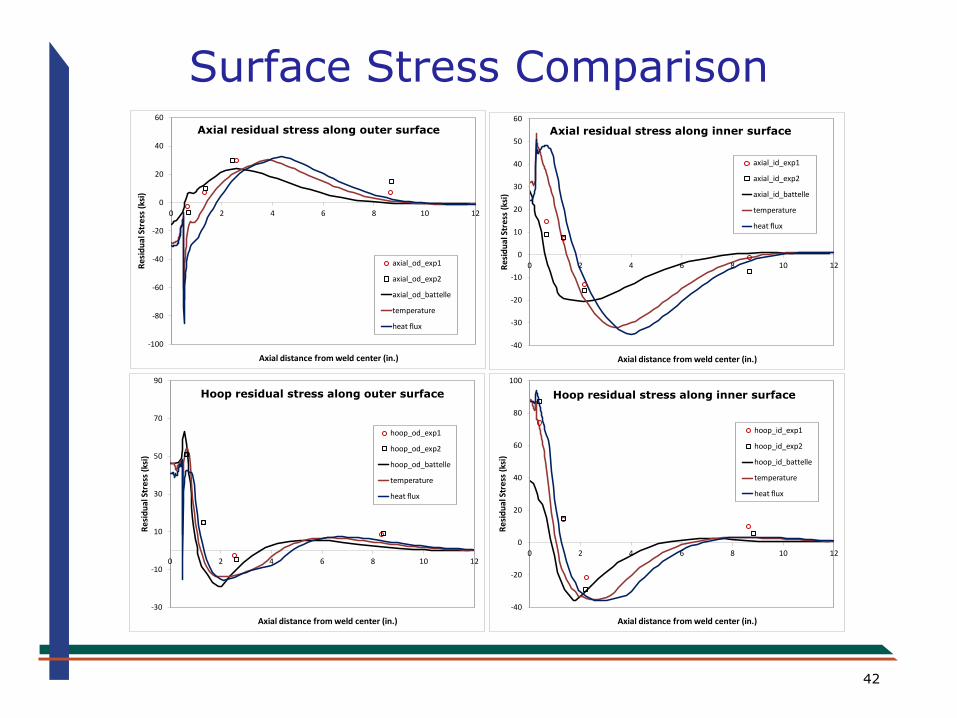
Surface Stress Comparison

-40

-30

-20

-10

0

10

20

30

40

50

60

0 2 4 6 8 10 12Re

sid

ual

Str

ess

(ks

i)

Axial distance from weld center (in.)

axial_id_exp1

axial_id_exp2

axial_id_battelle

temperature

heat flux

Axial residual stress along inner surface

-100

-80

-60

-40

-20

0

20

40

60

0 2 4 6 8 10 12

Re

sid

ual

Str

ess

(ks

i)


axial_od_exp1

axial_od_exp2

axial_od_battelle

temperature

heat flux

Axial residual stress along outer surface

-30

-10

10

30

50

70

90

0 2 4 6 8 10 12

Re

sid

ual

Str

ess

(ks

i)


hoop_od_exp1

hoop_od_exp2

hoop_od_battelle

temperature

heat flux

-40

-20

0

20

40

60

80

100

0 2 4 6 8 10 12

Re

sid

ual

Str

ess

(ks

i)


hoop_id_exp1

hoop_id_exp2

hoop_id_battelle

temperature

heat flux

Hoop residual stress along inner surface Hoop residual stress along outer surface

43

Weld Linearized Stress

• S22 is pipe axial stress, S33 is pipe hoop stress

-40000

-20000

0

20000

40000

60000

80000

100000

0 0.2 0.4 0.6 0.8 1

Stre

ss (p

si)

Distance Along Linearization Line (from ID, inches)

S22 DLUX

S22 M+B DFLUX

S22 TEMPERATURE

S22 M+B TEMPERATURE

S33 DFLUX

S33 M+B DFLUX

S33 TEMPERATURE

S33 M+B TEMPERATURE

44

Base Linearized Stress

-100000

-80000

-60000

-40000

-20000

0

20000

40000

60000

80000

100000

0 0.1 0.2 0.3 0.4 0.5 0.6 0.7

Stre

ss (p

si)


S22 DLUX

S22 M+B DFLUX

S22 TEMPERATURE

S22 M+B TEMPERATURE

S33 DFLUX

S33 M+B DFLUX

S33 TEMPERATURE

S33 M+B TEMPERATURE

45

Base Linearized Stress

-60000

-40000

-20000

0

20000

40000

60000

80000

0 0.1 0.2 0.3 0.4 0.5 0.6 0.7

Stre

ss (p

si)


S22 DLUX

S22 M+B DFLUX

S22 TEMPERATURE

S22 M+B TEMPERATURE

S33 DFLUX

S33 M+B DFLUX

S33 TEMPERATURE

S33 M+B TEMPERATURE

46

Summary

• Differences of +20 ksi (tension) are typical in linearized stress between the thermal approaches, which seems non-trivial

• Based on this limited example, primary effect of assigned heat flux is larger and more realistic overall heat input, which increases stress magnitudes

– Heat flux balances the welding power input, even in 2D

– Typical temperature assignment approaches would be expected to significantly under-estimate the heat input

• However; general trends (through thickness and surface vs. distance) are more-or-less unchanged

• This suggests that the largest concern with using assigned temperature results is that the stresses will likely be indexed to a heat input potentially much greater than they actually represent

• Note that these conclusions are based on 2D analysis, and 3D analysis adds additional complexities

Documents

Verification of Welding Power Input in Two-Dimensional