Embed Size (px)
Citation preview
NREL is a national laboratory of the U.S. Department of Energy, Office of Energy Efficiency & Renewable Energy, operated by the Alliance for Sustainable Energy, LLC.
Contract No. DE-AC36-08GO28308
Verification and Validation of EnergyPlus Conduction Finite Difference and Phase Change Material Models for Opaque Wall Assemblies Paulo Cesar Tabares-Velasco, Craig Christensen, Marcus Bianchi*, and Chuck Booten
*Current Affiliation: Owens Corning
Technical Report NREL/TP-5500-55792 July 2012

NREL is a national laboratory of the U.S. Department of Energy, Office of Energy Efficiency & Renewable Energy, operated by the Alliance for Sustainable Energy, LLC.
National Renewable Energy Laboratory 15013 Denver West Parkway Golden, Colorado 80401 303-275-3000 • www.nrel.gov
Contract No. DE-AC36-08GO28308
Verification and Validation of EnergyPlus Conduction Finite Difference and Phase Change Material Models for Opaque Wall Assemblies Paulo Cesar Tabares-Velasco, Craig Christensen, Marcus Bianchi*, and Chuck Booten Prepared under Task No. BE12.0103
Technical Report NREL/TP-5500-55792 July 2012

NOTICE
This report was prepared as an account of work sponsored by an agency of the United States government. Neither the United States government nor any agency thereof, nor any of their employees, makes any warranty, express or implied, or assumes any legal liability or responsibility for the accuracy, completeness, or usefulness of any information, apparatus, product, or process disclosed, or represents that its use would not infringe privately owned rights. Reference herein to any specific commercial product, process, or service by trade name, trademark, manufacturer, or otherwise does not necessarily constitute or imply its endorsement, recommendation, or favoring by the United States government or any agency thereof. The views and opinions of authors expressed herein do not necessarily state or reflect those of the United States government or any agency thereof.
Available electronically at http://www.osti.gov/bridge
Available for a processing fee to U.S. Department of Energy and its contractors, in paper, from:
U.S. Department of Energy Office of Scientific and Technical Information P.O. Box 62 Oak Ridge, TN 37831-0062 phone: 865.576.8401 fax: 865.576.5728 email: mailto:[email protected]
Available for sale to the public, in paper, from:
U.S. Department of Commerce National Technical Information Service 5285 Port Royal Road Springfield, VA 22161 phone: 800.553.6847 fax: 703.605.6900 email: [email protected] online ordering: http://www.ntis.gov/help/ordermethods.aspx
Cover Photos: (left to right) PIX 16416, PIX 17423, PIX 16560, PIX 17613, PIX 17436, PIX 17721
Printed on paper containing at least 50% wastepaper, including 10% post consumer waste.

iii
Acknowledgments This work was supported by the U.S. Department of Energy under Contract No. DE-AC36-08-GO28308 with the National Renewable Energy Laboratory (NREL). The authors would like to thank Ben Polly and Dane Christensen of NREL, Therese Stovall of Oak Ridge National Laboratory, and Jan Kosny of Fraunhofer Center for Sustainable Energy Systems CSE for their critical reviews, and Ken Childs of Oak Ridge National Laboratory for providing comparative data from Heating 8.0.

iv
Executive Summary Phase change materials (PCMs) represent a potential technology to reduce peak loads and heating, ventilation, and air conditioning (HVAC) energy consumption in buildings. A few building energy simulation programs have the capability to simulate PCMs, but their accuracy has not been completely tested. This report summarizes NREL’s efforts to develop diagnostic test cases to conduct accurate energy simulations when PCMs are modeled in residential buildings. Overall, the procedure used to verify and validate the conduction finite difference (CondFD) and PCM models in EnergyPlus is similar to that dictated by American Society of Heating, Refrigerating and Air-Conditioning Engineers Standard 140, which consists of analytical verification, comparative testing, and empirical validation. Validation was done in two levels (wall or building) for the two algorithms (CondFD and PCM). The wall-level tests were very detailed and focused on a single wall subjected to particular boundary conditions on both sides for a relatively short duration. In contrast, the whole-house tests focused on an entire building, considering interactions between the building envelope, HVAC, and internal loads for periods that varied from a few days to a year. This process was valuable, as several bugs were identified and fixed in both models. EnergyPlus will use the validated CondFD and PCM models as a basis for version 7.1.
This study also includes a preliminary assessment of three residential building envelope technologies containing PCM: PCM-enhanced insulation, PCM-impregnated drywall, and thin PCM layers. These technologies are compared based on peak reduction and energy savings using the PCM and CondFD algorithm in EnergyPlus. Preliminary results using whole building energy analysis suggest that considerable annual energy savings up to 20% could be achieved using PCMs in residential buildings. However, careful design is needed to optimize PCM solutions according to the specific user goals for peak demand and energy use reductions. Optimum design should also include several variables such as PCM properties, location in the building envelope, and local climate. Future research will include more detailed parametric analyses to optimize the cost effectiveness of PCM wall strategies.

v
Definitions ASHRAE American Society of Heating, Refrigerating and Air-Conditioning
Engineers
CondFD Conduction finite difference
CTF Conduction transfer function
HVAC Heating, ventilation, and air conditioning
LinEnth Linear enthalpy curve
NonLinEnth Nonlinear enthalpy curve
NREL National Renewable Energy Laboratory
PCM Phase change material
Qin Inside heat flux
RMSE Root mean square error
Tin Inside surface temperature
Tmid Middle node temperature
vi
Table of Contents Acknowledgments ........................................................................................................................................ iii
Executive Summary ...................................................................................................................................... iv
Definitions ..................................................................................................................................................... v
Figures ......................................................................................................................................................... vii
Tables ......................................................................................................................................................... viii
1 Introduction .......................................................................................................................................... 1
2 EnergyPlus Phase Change Material Model ........................................................................................... 3
3 Verification and Validation ................................................................................................................... 5
3.1 Wall-Level Tests: CondFD .............................................................................................................. 5
3.2 Wall-Level Tests: Phase Change Materials .................................................................................... 6
3.2.1 Analytical Verification: Stefan Problem ................................................................................ 6
3.2.2 Comparative Testing Against Heating 7.3 ........................................................................... 10
3.2.3 Comparative Testing Against Heating 8.0 ........................................................................... 15
3.2.4 Experimental: DuPont Hot Box Experiment ........................................................................ 19
3.3 Building-Level Tests: Conduction Finite Difference .................................................................... 23
3.4 Building-Level Tests: Evaluation of Phase Change Material Model ............................................ 25
3.4.1 Phase Change Material Model Evaluation Using Modified ASHRAE Standard 140, Case 600 ............................................................................................................................. 25
3.4.2 PCM Model Evaluation Using BEopt New House ................................................................ 29
3.5 Conclusions From Verification and Validation ............................................................................ 31
4 Detailed Diagnostics Available for Whole Building Analysis for Phase Change Material Systems Using Verified Phase Change Material Model .............................................................................................. 32
5 Conclusions ......................................................................................................................................... 37
References .................................................................................................................................................. 38
Appendix A. Phase Change Material Properties Used in Experimental Validation .................................... 41
Appendix B. EnergyPlus Conduction Finite Difference and Phase Change Material Algorithms ............... 42

vii
Figures Figure 1. Outside surface heat flux calculated using analytical solution (analytical) and PCM model v6 for
three node spacing values (dx, dx/3, dx/9) ......................................................................................... 9 Figure 2. Node temperature 0.105 m from outside surface calculated using analytical solution
(analytical) and PCM model v6 for three node spacing values (dx, dx/3, dx/9). ................................ 9 Figure 3. Calculated PCM-Insulation middle node temperature (Tmid) using comparative software (H73),
EnergyPlus PCM model with default node spacing (E+), finer mesh (E+dx/3), 2- and 4-min time steps (E+2min, E+4min) and without PCM (E+NoPCM) .................................................................... 12
Figure 4. Inside surface temperature (Tin) calculated using comparative software (H73), EnergyPlus PCM model with default node spacing (E+), finer mesh (E+dx/3), 2- and 4-min time steps (E+2min, E+4min) and without PCM (E+NoPCM) ............................................................................................. 12
Figure 5. Inside heat flux (Qin) calculated using comparative software (H73), EnergyPlus PCM model with default node spacing (E+), finer mesh (E+dx/3), 2- and 4-min time steps (E+2min, E+4min) and without PCM (E+NoPCM). ................................................................................................................. 13
Figure 6. Enthalpy curve for PCM with linear enthalpy curve (LinEnth) and for PCM with nonlinear enthalpy curve (NonLinEnth) used in comparative testing against Heating 8.0 ............................... 15
Figure 7. Calculated PCM-insulation middle node temperature(Tmid) for PCM with linear enthalpy curve using Heating 8.0 explicit solution (H8_Ex), Heating 8.0 implicit solution (H8-Im), EnergyPlus PCM model v7.1 with default node spacing (E+), and EnergyPlus without PCM (E+NoPCM) .................. 16
Figure 8. Calculated PCM-Insulation Tmid for PCM with non linear enthalpy curve using the same legend as Figure 7 ......................................................................................................................................... 16
Figure 9. Calculated Tin for PCM with linear enthalpy curve using the same legend as Figure 7 ............... 17 Figure 10. Calculated Tin for PCM with non linear enthalpy curve using the same legend as Figure 7 ...... 17 Figure 11. Calculated Qin for PCM with linear enthalpy curve using the same legend as Figure 7 ............ 18 Figure 12. Calculated Qin for PCM with non linear enthalpy curve using the same legend as Figure 7 ..... 18 Figure 13. Tested wall configuration with dimensions (in cm) and location of temperature (Temp) and
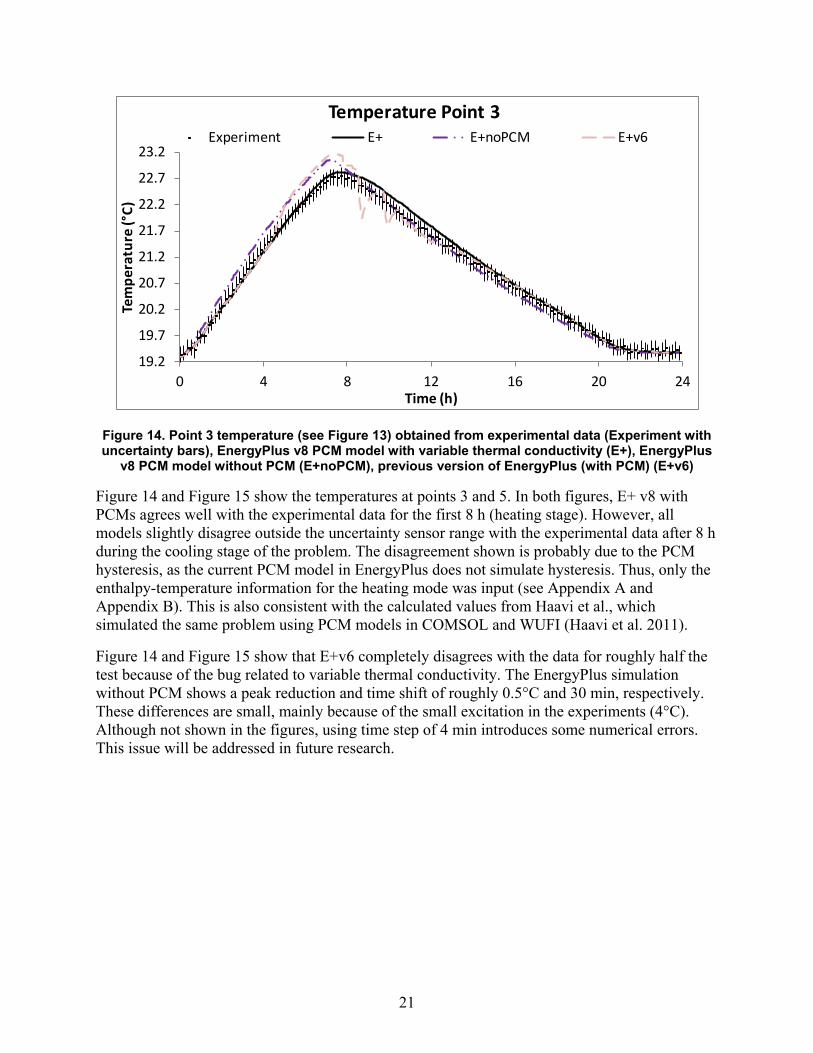
heat flux measurements (HF) ............................................................................................................ 20 Figure 14. Point 3 temperature (see Figure 13) obtained from experimental data (Experiment with
uncertainty bars), EnergyPlus v8 PCM model with variable thermal conductivity (E+), EnergyPlus v8 PCM model without PCM (E+noPCM), previous version of EnergyPlus (with PCM) (E+v6) ......... 21
Figure 15. Point 5 temperature (see Figure 13) obtained from experimental data (Experiment), EnergyPlus v8 PCM model with variable thermal conductivity (E+), EnergyPlus v8 PCM model without PCM (E+noPCM), previous version of EnergyPlus (v6) ........................................................ 22
Figure 16. Point 5 heat flux obtained from: experimental data (Experiment), EnergyPlus PCM model with variable thermal conductivity (E+), EnergyPlus PCM model without PCM (E+noPCM), and previous version of EnergyPlus (v6) ................................................................................................................. 23
Figure 17. Rendering of BEopt new house simulated ................................................................................. 24 Figure 18. 3-Day Cooling Energy use calculated with EnergyPlus using the CTF and CondFD algorithms.
The green line represents differences between the algorithms, with values displayed on the right-Y axis. ........................................................................................................................................ 25

viii
Figure 19. Runtime for lightweight construction using EnergyPlus: v6 (E+v6), v8 (E+V8), v8 with a finer mesh (E+v8 dx/3), v8 with a 2-min (E+v8 2min), and a 4-min time step (E+v8 4min). The Y-axis represents CTFs without PCM (CTF), CondFD without PCM (CondFD), CondFD with PCM distributed in insulation (Insulation), CondFD with PCM between two insulation layers (Ins/PCM/Ins), and CondFD with PCM distributed in drywall (Drywall). ......................................................................... 28
Figure 20. Model evaluation results for annual cooling energy difference using legends as in Figure 19 ............................................................................................................................................ 29
Figure 21. Model evaluation results for monthly cooling electric energy difference for BEopt house using melting ranges specified in Table 9 for Phoenix, Arizona: upper half (Upper Attic) and lower half (Lower Attic) of the attic insulation with PCM, PCM concentrated at the middle of the attic insulation (RCRAttic), wall cavity with PCM distributed in insulation (Walls), PCM concentrated at the middle of the wall cavity insulation (RCRWall), PCM distributed drywall (Drywall) and combination of RCRWall and PCM-Drywall (RCRWall-DW) .............................................................. 30
Figure 22. Model evaluation results for monthly peak cooling electric difference for BEopt house using melting ranges specified in Table 9 for Phoenix, Arizona, using same captions as in Figure 21 ..... 31
Figure 23. Predicted cooling energy savings for multiple PCM strategies for a BEopt house in Phoenix .............................................................................................................................................. 32
Figure 24. Predicted peak cooling reduction for multiple PCM strategies for a BEopt house in Phoenix .............................................................................................................................................. 33
Figure 25. Predicted hourly energy savings from multiple PCM wall applications in April in Phoenix. Right Y-axis shows hourly energy use for house without PCMs (CoolingEner). ............................... 34
Figure 26. Predicted hourly energy savings from multiple PCM wall applications in July in Phoenix. Right Y-axis shows hourly energy use for house without PCMs (CoolingEner). ............................... 35
Figure 27. Predicted heating energy savings from different PCM strategies ............................................. 36
Tables Table 1. Verification and Validation Procedure ............................................................................................ 5 Table 2. Properties of PCM Strategies Analyzed ........................................................................................... 7 Table 3. Properties of PCM Strategies Analyzed in Comparative Verification ........................................... 11 Table 4. Root Mean Square Error (RMSE) Compared to Heating 7.3 Values for PCM Distributed in
Insulation ........................................................................................................................................... 14 Table 5. Differences in Net Heat Gain Over 12 Hours Between Heating 7.3 and Other Models ............... 14 Table 6. RMSE for PCM Distributed in Drywall Compared to Heating 7.3 .................................................. 14 Table 7. RMSE Compared to Heating 8.0 Explicit Solution Values for PCM Distributed in insulation ........ 19 Table 8. Modified Case 600 Materials Properties ....................................................................................... 26 Table 9. Properties of PCM Strategies Analyzed ......................................................................................... 26 Table 10. Thermal Storage of Composite PCMs for Modified House ASHRAE Standard 140, Case 600 .... 27 Table 11. Thermal Storage of Composite PCMs for BEopt New House ...................................................... 30

1
1 Introduction Energy can be stored in buildings via sensible, latent, or chemical means. Of these, latent storage using phase change materials (PCMs) has been the focus of multiple building studies and companies because of its greater potential thermal energy storage density compared to sensible storage. Multiple PCMs are commercially available that vary in type (salts, paraffins, fatty acids), encapsulation technology (micro and macro encapsulation), and melting temperatures (covering a range that is useful for building wallboard and enclosure applications (64°–104oF [18°–40oC]).
PCMs represent a potential technology for reducing peak loads and heating, ventilation, and air conditioning (HVAC) energy consumption in buildings. Research on PCMs has considered many heat transfer applications during the last two decades, resulting in a considerable amount of literature about PCM properties, indoor temperature stabilization potential, and peak load reduction potential. Buildings PCM-oriented research has investigated two primary applications: passive and active building systems (Khudhair & Farid 2004; Pasupathy, Velraj & Seeniraj 2008; Tyagi & Buddhi 2007; Sharma, Tyagi, Chen & Buddhi 2009; Wang, Zhang, Xiao, Zeng, Zhang & Di 2009). Previous PCM studies have shown important benefits related to thermal comfort, energy savings, and perhaps HVAC downsizing when thermal storage is added into buildings (Zhu, Ma & Wang 2009).
Early numerical studies analyzed PCM wallboards during the late 1970s and 1980s, mainly for PCM-impregnated wallboard applications (Drake 1987; Solomon 1979). Later numerical studies used PCM thermal properties obtained from differential scanning calorimetry techniques and from measurements of temperature profiles across impregnated PCM wallboard (Kedl 1990; Athienitis et al. 1997). More recent studies of PCM wallboards have analyzed building elements containing microencapsulated PCM. One study compared the performance of a detailed model considering a solid-liquid interface against a simpler model using an equivalent heat capacity model. Overall, the equivalent heat capacity method performed better compared to experimental data (Ahmad, Bontemps, Sallée and Quenard 2006). Another study found the optimum time and space steps for a specific PCM using the heat capacity method, differential scanning calorimetry material property data, and an implicit finite difference model (Kuznik, Virgone & Roux 2008). A follow up study concluded that hysteresis should be considered in the numerical simulations to improve the overall accuracy of the model (Kuznik & Virgone 2009). Numerical research about PCM-enhanced building enclosure systems has followed a similar approach to that used for the wallboard arrangements, analyzing a building enclosure system containing PCM between two layers of insulation (Petrie, Childs, Christian, Childs & Shramo 1997; Halford & Boehm 2007).
These studies focused on understanding the physics behind PCMs, including validating models and investigating heat flux reduction potential using special laboratory and small-scale test rooms. Other studies have attempted to estimate potential energy savings through building energy simulation. Energy simulation studies analyzing energy and peak load benefits from PCMs have used commercial building energy simulation software such as CoDyBa (Virgone et al. 2009), ESP-r (Heim & Clarke 2004; Schossig, Henning, Gschwandera & Haussmann 2005; Heim 2010), and TRNSYS (Stovall & Tomlinson 1995; Koschenz & Lehmann 2004; Ibáñez, Lázaro, Zalba & Cabeza 2005). The implemented models varied from early PCM models (Tomlinson & Heberle 1990; Stovall & Tomlinson 1995), to empirical models using an

2
equivalent heat transfer coefficient (Ibáñez et al. 2005), to fully implemented finite difference models (Koschenz & Lehmann 2004; Pedersen 2007) and control volumes models (Heim & Clarke 2004). Predictions from these studies included no significant energy benefits (Pedersen 2007); improved thermal comfort and decreased peak load (Tomlinson & Heberle 1990; Stovall &Tomlinson 1995); and 90% reduction of heating energy demand during the heating season (Heim& Clarke 2004). Likewise, an energy simulation study focusing on building enclosure systems predicted 19%–57% peak load reduction for an attic system consisting of a PCM sandwiched between two conventional insulation layers (Halford & Boehm 2007).
In conclusion, PCMs have different benefits depending on their quantity and type (phase change temperature, energy storage capacity), location (drywall, walls, attic, and floor) and climate (heating and/or cooling performance). Therefore, there are clear differences between the methods and results from previous research efforts as: (1) most of the reviewed building energy simulation studies did not perform comprehensive model PCM validation (except a TRNSYS model that works for certain exterior PCM applications) (Kuznik et al. 2008); and (2) previous studies do not cover a wide range of PCM types, locations, and climates. Thus, there is a simulation and analysis gap with respect to PCM benefits and modeling. As a result, the objective of this study is to verify, validate, and improve (if necessary) the EnergyPlus PCM model that has yet not been fully validated. This procedure will be performed using analytical and comparative verifications and empirical validation of three PCM applications:
• PCM distributed in drywall
• PCM distributed in fibrous insulation
• Thin, concentrated PCM layers.
3
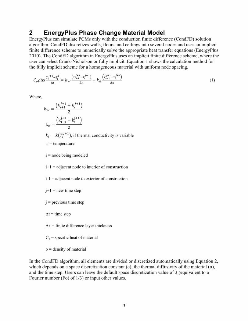
2 EnergyPlus Phase Change Material Model EnergyPlus can simulate PCMs only with the conduction finite difference (CondFD) solution algorithm. CondFD discretizes walls, floors, and ceilings into several nodes and uses an implicit finite difference scheme to numerically solve the appropriate heat transfer equations (EnergyPlus 2010). The CondFD algorithm in EnergyPlus uses an implicit finite difference scheme, where the user can select Crank-Nicholson or fully implicit. Equation 1 shows the calculation method for the fully implicit scheme for a homogeneous material with uniform node spacing.
𝐶𝑝𝜌Δx 𝑇𝑖𝑗+1−𝑇𝑖
𝑗
Δ𝑡= 𝑘𝑊
�𝑇𝑖+1𝑗+1−𝑇𝑖
𝑗+1�
Δx+ 𝑘𝐸
�𝑇𝑖−1𝑗+1−𝑇𝑖
𝑗+1�
Δx (1)
Where,
𝑘𝑊 =�𝑘𝑖+1
𝑗+1 + 𝑘𝑖𝑗+1�
2
kE =�ki−1
j+1 + kij+1�
2
𝑘𝑖 = 𝑘�𝑇𝑖𝑗+1�, if thermal conductivity is variable
T = temperature
i = node being modeled
i+1 = adjacent node to interior of construction
i-1 = adjacent node to exterior of construction
j+1 = new time step
j = previous time step
Δt = time step
Δx = finite difference layer thickness
Cp = specific heat of material
ρ = density of material
In the CondFD algorithm, all elements are divided or discretized automatically using Equation 2, which depends on a space discretization constant (c), the thermal diffusivity of the material (α), and the time step. Users can leave the default space discretization value of 3 (equivalent to a Fourier number (Fo) of 1/3) or input other values.

4
Δx = √c ∙ α ∙ Δt = �α∙ ΔtFo
(2)
For the PCM algorithm, the CondFD method is coupled with an enthalpy-temperature function (Equation 3) that the user inputs to account for enthalpy changes during phase change (Pedersen 2007). The enthalpy-temperature function is used to develop an equivalent specific heat at each time step. The resulting model is a modified version of the enthalpy method (Pedersen 2007).
h = h(T) (3)
Cp∗(T) = hij−hi
j−1
Tij−Ti
j−1 (4)
Where
h = enthalpy

5
3 Verification and Validation Accurate modeling of PCMs requires validation of the PCM and CondFD algorithms. This validation work is being completed at the National Renewable Energy Laboratory (NREL) following American Society of Heating, Refrigerating and Air-Conditioning Engineers (ASHRAE) Standard 140 and NREL validation methodologies, which consist of analytical verification, comparative testing, and empirical validation (Judkoff & Neymark 2006). Fixes in EnergyPlus were gradually implemented as they were fixed: from version 5 to the 2012 release version 7.1. The final PCM model considered for verification and validation is a modified version of EnergyPlus 6.0.0.037 that includes all fixes from the CondFD verification (Tabares-Velasco & Griffith 2011). This version will be referred as “v6” in this report. The new and improved PCM/CondFD model will be referred as version “v8,” or “v7.1” as the fixes that will be described later in this publication were not included in the 2011 EnergyPlus version 7 release due to time constraints. The fully validated model in EnergyPlus is included in v7.1. Validation was done in two levels (wall or building) with the two algorithms (CondFD and PCM), as shown in Table 1.
3.1 Wall-Level Tests: CondFD The wall-level tests were very detailed tests that focused on a single wall subjected to particular boundary conditions on both sides for a relatively short time. Thus, the wall-level validation tested the ability of only the specific CondFD and PCM algorithms to accurately model building envelope applications).
1Heating 7.3 is a multidimensional, finite difference heat conduction program that can simulate materials with variable thermal properties and other features. 2ANSI/ASHRAE Standard 140-2004: Standard Method of Test for the Evaluation of Building Energy Analysis Computer Programs. 3EnergyPlus models were generated using Building Energy Optimization (BEopt) according to the Building America 2010 Benchmark.
Table 1. Verification and Validation Procedure
Verification/Validation Level CondFD PCM
Wall
Analytical: • Variable k • Composite wall • Const heat flux (2) • Periodic BC • Symmetry
Comparative: • H7.3 transient variable k • H7.3 transient multilayer wall
Analytical: • Stefan Problem
Comparative: • Heating 7.31
Empirical: • DuPont Hotbox
Building
Comparative: • ASHRAE 140 Case 6002 • BEopt retrofit house • BEopt new house3
Evaluation: • ASHRAE 140 Case 600 • BEopt new house

6
The wall-level tests shown in Table 1 for CondFD consisted of eight test cases that were found to be useful for quality control of energy simulation models. In these cases CondFD was examined, debugged, and verified using these test cases. All test cases relate to diagnosing errors in conduction heat flux algorithms and how they interact with respective boundary conditions. The test cases tend to resemble laboratory-based heat transfer experiments on a single surface rather than a full thermal zone that resembles a building or thermal test cell. The proposed test cases offer additional diagnostic power for repairing coding errors in the area of variable thermal conductivity, Neumann boundary conditions, and transient boundary conditions. These additional test cases complement ASHRAE 140 and ASHRAE 1052-RP and are useful additions to that standard method of test.
Overall, more than six programming bugs were found and fixed that ranged from minor incorrect reporting of some variables to more serious problems in the CondFD model, including: (1) stability issues caused by the time marching scheme; (2) improper thermal conductivity evaluation when it is variable; and (3) incorrect timing for when the transient history terms are updated. The authors have also added to EnergyPlus version 7 the ability to control the following features: (1) the time marching scheme (Crank-Nicholson or fully implicit); (2) the value of the constant (“3” in Equation 1) used to set space discretization, by essentially making the inverse of the Fourier number an input; and (3) values for the maximum and minimum limits for convection surface heat transfer coefficients (Tabares-Velasco and Griffith 2011). Appendix B shows input settings for CondFD.
3.2 Wall-Level Tests: Phase Change Materials The wall-level tests shown in Table 1 for PCMs consisted of three test cases representing analytical verification, comparative testing, and empirical validation. Thus, the PCM model was verified using: (1) an analytical solution from the Stefan Problem as generalized by Franz Neumann (Carslaw & Jaeger 1959); (2) a numerical solution of a sine wave problem using a verified PCM model from Heating 7.3 (Childs 2005); and (3) experimental data from a hot box apparatus (Haavi, Gustavsen Cao, Uvsløkk & Jelle 2011). Moreover, the PCM model is tested for building envelope applications only, as heat diffusion and storage in the walls and attic were considered in the verification and validation. It is important to mention that: (1) the PCM model was not fully validated before; and (2) that the validation and verification process is not calibrating or evaluating the model, because the model input would not be changed or tuned as a result of the verification. As a result, the PCM verification and validation process found two programming bugs. The first caused stability problems with the EnergyPlus v6 PCM model and was fixed using an automatic under-relaxation factor. The other bug related to the simultaneous use of PCMs and variable thermal conductivity (Tabares-Velasco, Christensen & Bianchi 2012).
3.2.1 Analytical Verification: Stefan Problem The first verification test was the analytical solution to the “Stefan Problem” developed by Neumann for a semi-infinite wall. The solution assumptions are:
• The wall is initially at uniform temperature with PCM in the liquid form above the melting temperature (T(x,t)>Tmelting).
• Suddenly at time = 0, the wall outside surface temperature drops to 0oC (T(0,t)= 0oC).
7
• PCM density is equal and constant in both the liquid and solid phases.
• PCM thermal conductivity and specific heat are constant in each phase and can differ between the solid and liquid phases.
• PCM has a fixed melting temperature (no melting/freezing range) (Carslaw & Jaeger 1959).
The analytical solution was used to test the v6 PCM model for the three PCM applications, assuming the properties and characteristics shown in Table 2. Specific details include: (1) a simulated construction with one zone having only one wall; and (2) the walls were initially at a homogenous temperature of 50oC and had a melting temperature range of 29.4–29.6oC to approximate the fixed melting temperature assumption in the Stefan Problem. The semi-infinite wall was simulated by a thick wall, thus all surface temperatures were set in EnergyPlus using the “OtherSideCoefficient” feature; the indoor air temperature was set to the desired temperature and the inside convective heat coefficient was set to 1000 W/m2C. More details about similar approaches are in the literature (Tabares-Velasco & Griffith 2011).
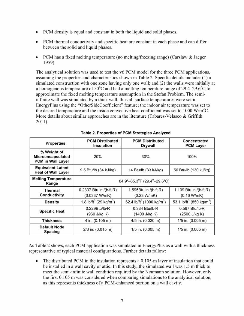
Table 2. Properties of PCM Strategies Analyzed
Properties PCM Distributed Insulation
PCM Distributed Drywall
Concentrated PCM Layer
% Weight of Microencapsulated PCM in Wall Layer
20% 30% 100%
Equivalent Latent Heat of Wall Layer 9.5 Btu/lb (34 kJ/kg) 14 Btu/lb (33 kJ/kg) 56 Btu/lb (130 kJ/kg)
Melting Temperature Range 84.9o–85.3oF (29.4o–29.6oC)
Thermal Conductivity
0.2337 Btu in./(h∙ft∙R) (0.0337 W/mK)
1.595Btu in./(h∙ft∙R) (0.23 W/mK)
1.109 Btu in./(h∙ft∙R) (0.16 W/mK)
Density 1.8 lb/ft3 (29 kg/m3) 62.4 lb/ft3 (1000 kg/m3) 53.1 lb/ft3 (850 kg/m3)
Specific Heat 0.229Btu/lb∙R (960 J/kg K)
0.334 Btu/lb∙R (1400 J/kg K)
0.597 Btu/lb∙R (2500 J/kg K)
Thickness 4 in. (0.105 m) 4/5 in. (0.020 m) 1/5 in. (0.005 m) Default Node
Spacing 2/3 in. (0.015 m) 1/5 in. (0.005 m) 1/5 in. (0.005 m)
As Table 2 shows, each PCM application was simulated in EnergyPlus as a wall with a thickness representative of typical material configurations. Further details follow:
• The distributed PCM in the insulation represents a 0.105-m layer of insulation that could be installed in a wall cavity or attic. In this study, the simulated wall was 1.5 m thick to meet the semi-infinite wall condition required by the Neumann solution. However, only the first 0.105 m was considered when comparing simulations to the analytical solution, as this represents thickness of a PCM-enhanced portion on a wall cavity.

8
• The distributed PCM in drywall represents a 0.02-m layer of drywall. In this study, the simulated wall was 0.3 m thick to meet the semi-infinite wall condition required by the Neumann solution. However, only the first 0.02 m was considered when comparing simulations to the analytical solution, as this represents the PCM-enhanced portion of the wall.
• The concentrated PCM represents a 0.005-m layer that could be installed between two layers of insulation or between insulation and drywall. In this study, the simulated wall contained only concentrated PCM and was 0.155 m thick to meet the semi-infinite wall condition required by the Neumann solution. However, only the first 0.005 m was considered when comparing simulations to the analytical solution, as this represents the PCM-enhanced portion of the wall.
All three numerical and analytical solutions show similar results; the PCM model also behaves similarly between cases. For this reason, detailed results are shown here for the PCM-enhanced insulation only. Figure 1 and Figure 2 show results for three node spacing values: 0.015 m (the default, dx), 0.005 m (dx/3), and 0.00167 m (dx/9), which are obtained using a Fourier number equal to 1/3, 3, and 26. These Fourier numbers seem high and would cause problems if an explicit scheme had been chosen. However, this study used the fully implicit scheme, which can work with higher Fourier numbers and steadily decays to convergence (Waters & Wright 1985; Hensen & Nakhi 1994).
Figure 1 shows how the v6 PCM model solution for the coarsest grid (dx) oscillates around the analytical solution: the temperature from the PCM model suddenly increases, followed by almost constant or flat behavior around the analytical solution. This behavior was observed at the coarsest node spacing value in each solution for the three PCM applications. It was also observed in each solution for the three PCM applications, but with a lesser magnitude, in the other node spacing cases (dx/3 and dx/9). The reason for this oscillatory behavior is mainly numerical; the solution to this problem requires a fine mesh to properly simulate heat wave propagation through the PCM with a fixed melting temperature.

9
Figure 1. Outside surface heat flux calculated using analytical solution (analytical) and PCM model v6 for three node spacing values (dx, dx/3, dx/9)
Figure 2. Node temperature 0.105 m from outside surface calculated using analytical solution (analytical) and PCM model v6 for three node spacing values (dx, dx/3, dx/9).
This study also analyzed the model stability and convergence by recording the number of iterations required for the PCM model to converge. In the three discretization cases, the solution did not converge when a node entered or left the melting range. Thus, after CondFD passed the maximum allowable iterations, the solution did not meet the convergence criteria. Therefore, the
-150
-130
-110
-90
-70
-50
-30
-10
1 11 21 31 41 51
Heat
Flux
(W/m
2 )
Time (min)
Analytical PCMv6 dx PCMv6 dx/3 PCMv6 dx/9
40
42
44
46
48
50
1 11 21 31 41 51
Tem
pera
ture
(o C)
Time (min)
Analytical PCMv6 dx PCMv6 dx/3 PCMv6 dx/9

10
PCM model used the values from the last iterations and moved to the next time step even though it did not converge. This problem did not cause any significant accuracy issues for the three cases tested because of the small time step used, but did increase the runtime significantly, taking 6, 15, and 66 min to simulate the wall for 2 days in the dx, dx/3, dx/9 scenarios, respectively.
The convergence problem was solved by adding an automatic and dynamic under-relaxation factor after a determined number of iterations. This new under-relaxation factor did not affect the accuracy of the PCM model and reduced the runtime 60%–90% relative to the v6 model. It is important to mention that the semi-infinite wall problem stated by the Neumann solution is very demanding and challenging from a numerical point of view. A very close match was obtained with only Heating 7.3, using a time step of 0.01 s and node spacing roughly 0.01 times the default size in EnergyPlus. These values are stricter than values that have been recommended in previous studies (Kuznik, Virgone & Johannes 2010); they are likely too strict and impractical for modeling more realistic PCM-enhanced wall configurations in annual building simulations. As a result, it is important to verify the PCM model with more realistic wall and boundary conditions. However, there is no analytical solution for this case, so comparative testing using another verified numerical model is needed.
3.2.2 Comparative Testing Against Heating 7.3 The analytical verification allowed for the detection of runtime issues and identification of node spacing requirements for an extreme circumstance with a large and sudden temperature drop. The last test is useful as a quality assurance tool but not for a performance-based tool. Thus, the next step in the verification process was comparative testing relative to the ideal PCM model in Heating 7.3. This model was also tested with the Neumann solution, thus proving the accuracy of the model at small time steps (0.01 s). The comparative verification consisted of a 24-h sine temperature wave test with amplitude of 30oC representing outside temperature variation during a day, and a 1-dimensional wall consisting of 1 cm wood, 10 cm fiber insulation, and 1.5 cm drywall. This test represents a more realistic wall configuration and boundary conditions than the analytical solution. Model space discretization and boundary conditions are:
• 0.01second time steps
• Node spacing 0.01 times the EnergyPlus default value
• Indoor air temperature: 25oC t ≥0
• Indoor convective heat transfer coefficient: hi=5W/m2K
• Outside air temperature: 25°C at t=0; varying sinusoidal over 24 h with a range 10°–40oC
• Outdoor convective heat transfer coefficient: hout=20W/m2K
• Wall initial conditions: homogenous temperature of 25oC
• Ideal/pure PCM with a fixed melting temperature.
The two wall applications verified in this test are shown in Table 3. This test evaluates only two applications, because no significant information was obtained from conducting three tests in the

11
analytical test. In addition, the concentrated thin PCM layer application will be tested with experimental data in Section 3.3.
Table 3. Properties of PCM Strategies Analyzed in Comparative Verification
Properties PCM Distributed Insulation
PCM Distributed Drywall
% Weight of PCM in Wall Layer 20% 30%
Equivalent Latent Heat 9.5 Btu/lb (34 kJ/kg) 14 Btu/lb (33 kJ/kg)
Melting Temperature 71oF (26oC) 69.6oF (25.05oC)
Thermal Conductivity 0.2337 Btu in./(h∙ft∙R)
(0.0337 W/mK) 1.595 Btu in./(h∙ft∙R)
(0.23 W/mK) Density 3.1 lb/ft3 (50 kg/m3) 59.3 lb/ft3 (950 kg/m3)
Specific Heat 0.229 Btu/lb∙R (960 J/kg K) 0.20 Btu/lb∙R (840 J/kg K)
Thickness 4 in. (0.105 m) 3/5 in. (0.015 m) Default Node Spacing 2/3 in. (0.015 m) 1/5 in. (0.005 m)
Figure 3 through Figure 5 show the results of the comparative verification for the distributed PCM in insulation. All figures show calculated values using Heating 7.3 (H73), EnergyPlus v8 PCM model with default space discretization and 1-min time step (E+), EnergyPlus v8 with no PCM and 1-min time step (E+NoPCM), EnergyPlus v8 PCM model with finer mesh (E+dx/3) and 1-min time step, EnergyPlus v8 PCM model using a 2-min time step (E+2min), and EnergyPlus v8 PCM model using a 4-min time step (E+4min). Simulations with 2- and 4-min time steps used the default space discretization values. All EnergyPlus simulations were performed using use the updated model (v8). Additionally, Figure 3 through Figure 5 show that discrepancies increase substantially when time steps ≥4 min (E+4min) are used. Thus, all simulations should use time steps <4 min. Finally, Figure 3 through Figure 5 also show that the default space discretization (E+) and finer mesh (E+dx/3) closely agree with Heating 7.3.
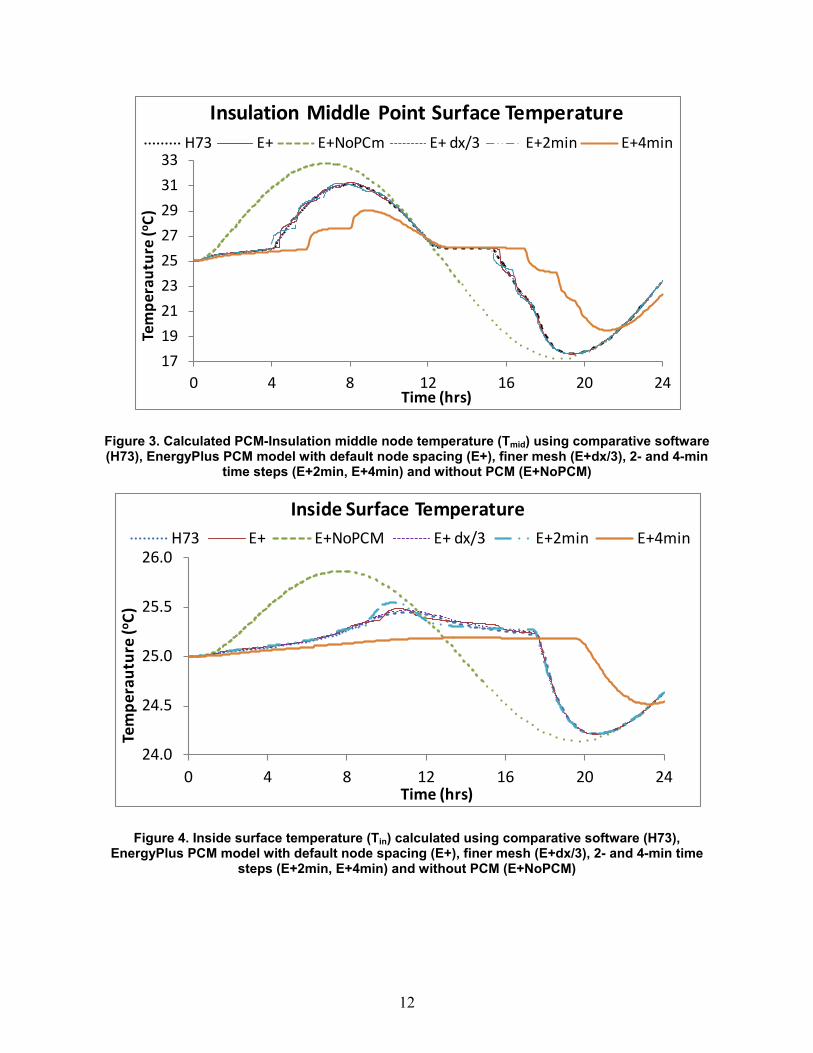
12
Figure 3. Calculated PCM-Insulation middle node temperature (Tmid) using comparative software (H73), EnergyPlus PCM model with default node spacing (E+), finer mesh (E+dx/3), 2- and 4-min
time steps (E+2min, E+4min) and without PCM (E+NoPCM)
Figure 4. Inside surface temperature (Tin) calculated using comparative software (H73), EnergyPlus PCM model with default node spacing (E+), finer mesh (E+dx/3), 2- and 4-min time
steps (E+2min, E+4min) and without PCM (E+NoPCM)
171921232527293133
0 4 8 12 16 20 24
Tem
pera
utur
e (o C
)
Time (hrs)
Insulation Middle Point Surface TemperatureH73 E+ E+NoPCm E+ dx/3 E+2min E+4min
24.0
24.5
25.0
25.5
26.0
0 4 8 12 16 20 24
Tem
pera
utur
e (o C
)
Time (hrs)
Inside Surface TemperatureH73 E+ E+NoPCM E+ dx/3 E+2min E+4min

13
Figure 5. Inside heat flux (Qin) calculated using comparative software (H73), EnergyPlus PCM model with default node spacing (E+), finer mesh (E+dx/3), 2- and 4-min time steps (E+2min,
E+4min) and without PCM (E+NoPCM).
Figure 3 also shows the temperature of the node in the middle of the insulation layer (Tmid). All node locations for this node are in the middle of the insulation except those for the 2-min (E+2min) and 4-min (E+4min) time steps, which were linearly interpolated as the automatic meshing in EnergyPlus did not generate a node in the middle of the insulation. Figure 3 and Figure 4 show that the node temperature calculated by the EnergyPlus PCM model oscillates around the temperature calculated by Heating 7.3. This is the same behavior observed in the analytical test. The oscillations attenuated and disappeared once a finer mesh was used, which in this case was about one third smaller node spacing than the default size. Furthermore, the selection of one third smaller node distance in EnergyPlus produced results nearly equal to Heating 7.3 results. Moreover, Figure 3 shows that during approximately the first 4 h the middle wall node temperature with PCM remained almost at constant temperature around the melting temperature (26oC). Once all the PCM has melted, the temperature started to increase as no more latent storage is available, delaying the peak temperature by almost 2 h. Overall, the benefits of PCM in this particular example are reflected in Figure 4 and Figure 5 where the peak inside surface temperature and heat flux are attenuated by 0.5oC and 50%, respectively, and the peak time is delayed almost 4 h.
Figure 4 and Figure 5 show the impact distributing PCM in the insulation has on the inner surface temperature and inside heat flux for this particular example. The peak load reduction and shift are correctly calculated by the PCM model. Despite the small oscillations around the values calculated from Heating 7.3, the PCM model with default space discretization obtains values close to Heating 7.3 (see Table 4). Moreover, using finer mesh improves the agreement with Heating 7.3 and the 2-min time step still has close agreement with Heating 7.3.
-5
-3
-1
1
3
5
0 4 8 12 16 20 24
Heat
Flux
(W/m
2 )
Time (hrs)
Inside Heat FluxH73 E+ E+NoPCM E+ dx/3 E+2min E+4min
14
Table 4. Root Mean Square Error (RMSE) Compared to Heating 7.3 Values for PCM Distributed in Insulation
Tin (oC)
Tmin (oC)
Qin (W/m2)
Qout (W/m2)
E+NoPCM 0.45290 2.6470 2.2940 4.370 E+ 0.01919 0.1384 0.1406 1.885
E+ dx/3 0.01564 0.0741 0.0771 0.357 E+2min 0.03715 0.2180 0.2698 0.717 E+4min 0.30770 2.3040 1.4590 2.844
Finally, Table 5 summarizes the discrepancies in the first 12-h cycle using the same caption labels as Figure 3. The results agree with Table 4; the default space discretization (E+) and smaller node spacing (E+dx/3) models with PCM agree with Heating 7.3 very closely. The 2-min time step (E+2min) has looser agreement but is still close compared to the case without PCM. The 4-min time step does not produce matching results. The comparison with EnergyPlus without PCM is just as a reference for completeness.
Table 5. Differences in Net Heat Gain Over 12 Hours Between Heating 7.3 and Other Models
Case Outside Heat Gain (kJ)
Inside Heat Gain (kJ)
Outside Discrepancy With
H7.3 (%) Inside Discrepancy
With H7.3 (%)
Heating 7.3 216 43 – – E+ 213 43 1.3% –1.5%
E+ dx/3 215 43 0.6% –0.7% E+2min 214 46 0.9% –7.8% E+4min 297 18 –37.6% 58.5%
E+ noPCM 127 115
The PCM model for the case with PCM distributed in the drywall has similar performance to the one shown in Table 4. Thus, only Table 6 is shown here, which shows that all cases agree, having an almost zero heat flux coming into the inside wall over a 24-h period.
Table 6. RMSE for PCM Distributed in Drywall Compared to Heating 7.3
Tin (oC)
Tmid (oC)
Qin (W/m2)
Qout (W/m2)
E+NoPCM 5.6180 3.066 4.610 1.801 E+ 0.0254 0.138 0.019 1.800
E+ dx/3 0.0255 0.114 0.017 0.347 E+2min 0.0257 0.015 0.193 1.777 E+4min 0.0340 0.753 0.197 4.394

15
3.2.3 Comparative Testing Against Heating 8.0 A second set of comparative tests used results from Heating 8.0, the latest version of Heating, which is currently an internal version at Oak Ridge National Laboratory. It has enhanced capabilities for PCMs, as it can model PCMs with linear and nonlinear enthalpy curves (Childs and Stovall, 2012). This comparative testing uses the same wall as described in Section 3.2.2 for the PCM distributed in insulation. However, this test uses a PCM with linear enthalpy curve (LinEnth) and a PCM with a more realistic nonlinear enthalpy profile (NonLinEnth) as shown in Figure 6. For these particular cases, the results of the EnergyPlus PCM model using the default node spacing value were compared to two solutions in Heating 8.0: an explicit solution with a time step of 0.25 s and an implicit solution with a time step of 60 s.
Figure 6. Enthalpy curve for PCM with linear enthalpy curve (LinEnth) and for PCM with nonlinear enthalpy curve (NonLinEnth) used in comparative testing against Heating 8.0
This comparative test used the same testing points as in Section 3.2.2: middle point inside insulation (Tmid), inside surface temperatures (Tin), and inside heat flux (). Figure 7 and Figure 8 show the Tmid for the PCM with LinEnth and NonLinEnth, respectively. Figure 9 and Figure 10 show the Tin for the PCM with LinEnth and NonLinEnth, respectively. Finally, Figure 11 and Figure 12 show Qin for the PCM with LinEnth and NonLinEnth, respectively. In all cases, the agreement between EnergyPlus and Heating 8.0 (implicit and explicit solutions) is nearly identical and overall agree more closely than in the case for Heating 7.3. The closer agreement is mainly due to the more realistic phase change range in Heating 8.0 instead of the ideal fixed phase change temperature used in Heating 7.3, which is harder to calculate numerically. In the case with these two PCMs with a phase change temperature change, none of the solutions with E+ showed the oscillatory behavior observed in the analytical solution and Heating 7.3 tests.
Figure 3 to Figure 5 and Figure 7 to Figure 12 show how the performance of PCMs changes based on the phase change temperature. All these PCMs had the same thermal properties, latent heat, and subjected to the same boundary and initial conditions. The only difference was on the phase change temperature range: from a fixed temperature to linear and non linear enthalpy
60
70
80
90
100
110
22 25 28 31 34
H (k
J/kg
)
Temperature (oC)
NonLinEnth LinEnth

16
profiles. This shows the importance of knowing correctly the characteristics of the PCM being analyzed.
Figure 7. Calculated PCM-insulation Tmid for PCM with linear enthalpy curve using Heating 8.0 explicit solution (H8_Ex), Heating 8.0 implicit solution (H8-Im), EnergyPlus PCM model v7.1 with
default node spacing (E+), and EnergyPlus without PCM (E+NoPCM)
Figure 8. Calculated PCM-Insulation Tmid for PCM with non linear enthalpy curve using the same legend as Figure 7
16182022242628303234
0 4 8 12 16 20 24
Tem
pera
ture
(o C)
Time (hrs)
H8-Ex H8-Im E+ E+noPCM
16182022242628303234
0 4 8 12 16 20 24
Tem
pera
ture
(o C)
Time (hrs)
H8-Ex H8-Im E+ E+NoPCM

17
Figure 9. Calculated Tin for PCM with linear enthalpy curve using the same legend as Figure 7
Figure 10. Calculated Tin for PCM with non linear enthalpy curve using the same legend as Figure 7
24.0
24.5
25.0
25.5
26.0
0 4 8 12 16 20 24
Tem
pera
ture
(o C)
Time (hrs)
H8-Ex H8-Im E+ E+NoPCM
24.0
24.5
25.0
25.5
26.0
0 4 8 12 16 20 24
Tem
pera
ture
(o C)
Time (hrs)
H8-Ex H8-Im E+ E+NoPCM

18
Figure 11. Calculated Qin for PCM with linear enthalpy curve using the same legend as Figure 7
Figure 12. Calculated Qin for PCM with non linear enthalpy curve using the same legend as Figure 7
Table 7 shows the RMSE for the EnergyPlus PCM model (linear and nonlinear PCM melt curve) and implicit solution of Heating 8.0 compared to the Heating 8.0 explicit solution. In most cases the EnergyPlus PCM models show very good agreement with the Heating 8.0 explicit solution as well as the implicit solution of Heating 8.0. This is true even though the time step for implicit solutions was 1 min and for explicit solutions it was 0.25 s. The good agreement between the
-5
-3
-1
1
3
5
0 4 8 12 16 20 24
Heat
Flux
(W/m
2 )
Time (hrs)
H8-Exp H8-Imp E+ noPCME+
-5
-3
-1
1
3
5
0 4 8 12 16 20 24
Heat
Flux
(W/m
2 )
Time (hrs)
H8-Exp H8-Imp E+ noPCME+
19
implicit and explicit solutions shows that under similar conditions EnergyPlus users can use the default space discretization value (which controls the relation between spatial and temporal discretization) without losing significant accuracy.
Table 7. RMSE Compared to Heating 8.0 Explicit Solution Values for PCM Distributed in insulation
Tin (oC)
Tmid (oC)
Qin (W/m2)
Qout (W/m2)
Heating 8.0 Implicit Linear PCM
0.003 0.004 0.267 0.021
E+ Linear PCM 0.008 0.033 0.267 0.149 Heating 8.0 Implicit
Non Linear PCM 0.003 0.004 0.009 0.018
E+ Non linear PCM 0.008 0.021 0.020 0.188
3.2.4 Experimental: DuPont Hot Box Experiment The last step in the verification and validation of the PCM model was empirical validation. This step compared the PCM model with experimental data from the literature (Cao et al. 2010; Haavi et al. 2011) for the concentrated PCM application. Figure 13 is a schematic of the wall tested with the PCM layer representing the DuPont Energain PCM product with a melting temperature range centered around 21.7°C, a latent heat of about 70 kJ/kg, and a variable thermal conductivity. Properties for this PCM are shown in Appendix A. It is important to mention that PCM properties in the experimental study were provided by the manufacturer; thus, there was there were no degrees of freedom to “calibrate” EnergyPlus results to match measured values. The tests were performed in a hot box apparatus where initially the cold box side was kept at –20°C and the hot side was kept at 20°C. At t=0, a heater in the hot box started heating the air temperature inside the hot box for 7 h (heating stage). The final inside wall temperature reached 24°C. After that, the heater was turned off and the hot box slowly cooled to the initial temperature, 20°C (cooling stage) (Cao et al. 2010; Haavi et al. 2011). Thus, based on the PCM properties listed in Appendix A, the PCM probably did not completely freeze and/or melt during an experimental cycle. However, the experimental results are still valid as long as they are understood to be representative of a situation where PCM might not completely melt during a 24-h diurnal cycle.

20
Figure 13. Tested wall configuration with dimensions (in cm) and location of temperature (Temp) and heat flux measurements (HF)
The initial comparison of the PCM model to the experimental data with variable thermal conductivity revealed another bug that occurred when these two features were simulated at the same time. This bug was fixed and Figure 14 to Figure 16 compare the results for the fixed version to the original, which is marked E+v6. Figure 14 to Figure 16 relate to the measurement points shown in Figure 13. Results from the empirical validation are shown in Figure 14 through Figure 16 for experimental data (Experiment) with the uncertainty bars, EnergyPlus v8 PCM model with variable thermal conductivity (E+), EnergyPlus v8 PCM model without PCM (E+noPCM), and the previous version of EnergyPlus (v6) with PCM. Although not shown in the figures, the PCM model was further evaluated using a 2-min time step, a 4-min time step, and a finer mesh (E+dx/3). These are not shown in Figure 14 to Figure 16 to avoid overpopulating the graphs; no results were observed that were not already described in Section 3.2. The 2-min time step with a finer mesh behaved similarly to the 1-min time step with default space discretization.
Point 3:Temp Point 7:
Temp
Gyps
umPC
M
Min
eral
Woo
l
Min
eral
Woo
l
Point 5:Temp & HF Point 11:
Temp
Hot Box Cold Box1.3
Point 1: Temp & HF
0.53 14.8 14.8
Gyps
um
0.9
21
Figure 14. Point 3 temperature (see Figure 13) obtained from experimental data (Experiment with uncertainty bars), EnergyPlus v8 PCM model with variable thermal conductivity (E+), EnergyPlus
v8 PCM model without PCM (E+noPCM), previous version of EnergyPlus (with PCM) (E+v6)
Figure 14 and Figure 15 show the temperatures at points 3 and 5. In both figures, E+ v8 with PCMs agrees well with the experimental data for the first 8 h (heating stage). However, all models slightly disagree outside the uncertainty sensor range with the experimental data after 8 h during the cooling stage of the problem. The disagreement shown is probably due to the PCM hysteresis, as the current PCM model in EnergyPlus does not simulate hysteresis. Thus, only the enthalpy-temperature information for the heating mode was input (see Appendix A and Appendix B). This is also consistent with the calculated values from Haavi et al., which simulated the same problem using PCM models in COMSOL and WUFI (Haavi et al. 2011).
Figure 14 and Figure 15 show that E+v6 completely disagrees with the data for roughly half the test because of the bug related to variable thermal conductivity. The EnergyPlus simulation without PCM shows a peak reduction and time shift of roughly 0.5°C and 30 min, respectively. These differences are small, mainly because of the small excitation in the experiments (4°C). Although not shown in the figures, using time step of 4 min introduces some numerical errors. This issue will be addressed in future research.
19.2
19.7
20.2
20.7
21.2
21.7
22.2
22.7
23.2
0 4 8 12 16 20 24
Tem
pera
ture
(°C)
Time (h)
Temperature Point 3Experiment E+ E+noPCM E+v6

22
Figure 15. Point 5 temperature (see Figure 13) obtained from experimental data (Experiment), EnergyPlus v8 PCM model with variable thermal conductivity (E+), EnergyPlus v8 PCM model
without PCM (E+noPCM), previous version of EnergyPlus (v6)
In addition to temperature data used for empirical validation, the experiments also measured heat fluxes. Figure 16 shows heat flux at measurement Point 5. Figure 16 shows that most models’ results are within the uncertainty range of the measured heat flux in Point 5 located between the PCM and mineral wood during the heating process. As with the results shown in Figure 14 and Figure 15, the disagreement increases once the PCM starts to cool and hysteresis occurs. In this case, the differences in the cooling range (starting around Time = 8 h) are on the order of 10%–15%. In all cases, the previous PCM model completely missed the behavior of the PCM because the bug had variable thermal conductivity.
19.0
19.5
20.0
20.5
21.0
21.5
22.0
22.5
23.0
0 4 8 12 16 20 24
Tem
pera
ture
(°C)
Time (h)
Temperature Point 5Experiment E+ E+noPCM E+v6

23
Figure 16. Point 5 heat flux obtained from: experimental data (Experiment), EnergyPlus PCM model with variable thermal conductivity (E+), EnergyPlus PCM model without PCM (E+noPCM),
and previous version of EnergyPlus (v6)
Overall, this comparison to empirical data was important because it tested the PCM model using a real PCM product with variable thermal conductivity. Combined, the results from Section 3.2 indicate that the v8 PCM model is performing well for PCM wall applications, except when the materials present strong hysteresis. The scope of this verification and the hysteresis limitation should be kept in mind when conducting whole-building simulations using EnergyPlus, such as those presented in the next section.
3.3 Building-Level Tests: Conduction Finite Difference The previous comparisons were important, but did not guarantee that the algorithms would work with more realistic situations and different HVAC systems. In contrast, the whole-house tests of this study focused on an entire building, considering interactions between the building envelope, HVAC, and internal loads for periods of time that vary from few days to a year. Building-level validation tests single-zone or multiple-zone houses and is mainly a comparison between conduction transfer functions (CTFs), which cannot be used with PCMs, and CondFD. Building-level verification compares hourly surface temperatures, average zone temperatures, hourly heating and cooling energy, and total heating and cooling energy between CondFD and CTFs.
• The comparative building-level verification for CondFD consisted of:
• ASHRAE Standard 140 Case 600: a simple one-zone building with lightweight construction (ASHRAE 2004).
• BEopt retrofit house: a one-story 1,280-ft2 (120-m2), 1960s-era house with three bedrooms, two bathrooms, and an unconditioned attic modeled in six of the eight original U.S. cities considered in previous retrofit analysis efforts (Polly et al. 2011).
3.4
3.6
3.8
4.0
4.2
4.4
4.6
4.8
5.0
0 4 8 12 16 20 24
Heat
Flux
(W/m
2 )
Time (h)
Heat Flux Point 5Experiment E+ E+noPCM E+v6
24
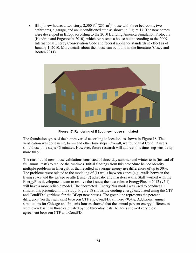
• BEopt new house: a two-story, 2,500-ft2 (231-m2) house with three bedrooms, two bathrooms, a garage, and an unconditioned attic as shown in Figure 17. The new homes were developed in BEopt according to the 2010 Building America Simulation Protocols (Hendron and Engebrecht 2010), which represents a house built according to the 2009 International Energy Conservation Code and federal appliance standards in effect as of January 1, 2010. More details about the house can be found in the literature (Casey and Booten 2011).
Figure 17. Rendering of BEopt new house simulated
The foundation types of the homes varied according to location, as shown in Figure 18. The verification was done using 1-min and other time steps. Overall, we found that CondFD users should use time steps ≤3 minutes. However, future research will address this time step sensitivity more fully.
The retrofit and new house validations consisted of three-day summer and winter tests (instead of full annual tests) to reduce the runtimes. Initial findings from this procedure helped identify multiple problems in EnergyPlus that resulted in average energy use differences of up to 30%. The problems were related to the modeling of (1) walls between zones (e.g., walls between the living space and the garage or attic); and (2) adiabatic and massless walls. Staff worked with the EnergyPlus development team to resolve the issues; the next release EnergyPlus in 2012 (v7.1) will have a more reliable model. The “corrected” EnergyPlus model was used to conduct all simulations presented in this study. Figure 18 shows the cooling energy calculated using the CTF and CondFD algorithms for the BEopt new houses. The green line represents the percent difference (on the right axis) between CTF and CondFD; all were <0.4%. Additional annual simulations for Chicago and Phoenix houses showed that the annual percent energy differences were even less than those calculated by the three-day tests. All tests showed very close agreement between CTF and CondFD.

25
Figure 18. 3-Day Cooling Energy use calculated with EnergyPlus using the CTF and CondFD algorithms. The green line represents differences between the algorithms, with values displayed
on the right-Y axis.
3.4 Building-Level Tests: Evaluation of Phase Change Material Model CondFD/PCM results could not be compared to the CTF results because PCMs cannot be modeled using the CTF algorithm. Thus, this work was called “evaluation” instead of “verification” (see Table 1). Nevertheless, the evaluation compared the runtimes and number of iterations required for CondFD to converge for different PCM applications as a measure to confirm models were converging without previous stability problems detected. The main purpose of this initial evaluation was to test and demonstrate the simulation capabilities of the PCM model in the context of whole buildings, not to draw conclusions about the performance of specific PCM technologies.
3.4.1 Phase Change Material Model Evaluation Using Modified ASHRAE Standard 140, Case 600
The Case 600 model was selected for its simplicity and because it is a well referenced and understood building that has been simulated by several major simulation engines (ASHRAE 2004). The basic test building is a lightweight, rectangular, single-zone building, with dimensions of 8 m × 6 m × 2.7 m. The building has no interior partitions, total window area of 12 m2 on the south wall, interior loads of 200 W (60% radiative, 40% convective) and a highly insulated slab to essentially eliminate thermal ground coupling. The infiltration was set to 0.5 air changes per hour. The building mechanical system is an ideal system with 100% convective air system and an efficiency of 100% with no duct losses and no capacity limitation. The thermostat is set with a deadband so heating takes place for temperatures below 20°C and cooling for temperatures above 27°C. Insulation properties have been slightly modified to incorporate PCMs (see Table 8 and Table 9). In contrast with the PCMs modeled in Section 3.2, all PCMs in Table 9 are assumed to have a 2oC melting temperature range. These three PCM cases represent
-0.1%
0.0%
0.1%
0.2%
0.3%
0.4%
0
50
100
150
Chicago Seattle Atlanta LA Houston Phoenix
Diffe
renc
e (%
)
Cool
ing
Ener
gy (k
Wh)
Location
3-DAY Cooling Energy UseCTF CondFD %Diff
Basement Crawlspace Slab
26
products that are already on the market or that have been previously investigated (Kedl 1990; Kosny et al. 2010a; Kosny, Shrestha, Stovall and Yarbrough, 2010b).
Table 8. Modified Case 600 Materials Properties
Material Thermal
Conductivity (W/m K)
Thickness (m)
Density (Kg/m3)
Specific Heat
(J/kg K)
Wall Plasterboard 0.1600 0.0120 950 840
Insulation 0.03365 0.0660 29 960 Wood siding 0.1400 0.0090 530 900
Roof Plasterboard 0.1600 0.0100 950 840
Insulation 0.03365 0.1118 29 960 Roof deck 0.1400 0.0190 530 900
Floor Timber flooring 0.1600 0.0100 950 840
Insulation 0.0400 0.2500 12 840
Table 9. Properties of PCM Strategies Analyzed
Properties PCM
Distributed Insulation
PCM Distributed Drywall
Concentrated PCM Layer
% Weight of Microencapsulated PCM in
Wall Layer 20% 30% 100%
Equivalent Latent Heat 9.5 Btu/lb (34 kJ/kg)
14 Btu/lb (33 kJ/kg)
56 Btu/lb (130 kJ/kg)
Melting Temperature Range 83°–87°F (28.5°–30.5°C)
72°–76°F (22.5°–24.5°C)
83°–87°F (28.5°–30.5°C)
Thermal Conductivity 0.234 Btu in./(h∙ft∙ R)
(0.0337 W/mK) 1.595 Btu in./(h∙ft∙R)
(0.23 W/mK) 1.109 Btu in./(h∙ft∙R)
(0.16 W/mK)
Density 1.8 lb/ft3
(29 kg/m3) 62.4 lb/ft3
(1000 kg/m3) 53.1 lb/ft3
(850 kg/m3)
Specific Heat 0.229 Btu/lb∙R (960 J/kg K)
0.334 Btu/lb∙R (1400 J/kg K)
0.597 Btu/lb∙R (2500 J/kg K)
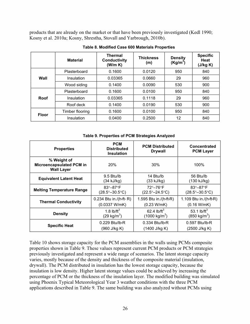
Table 10 shows storage capacity for the PCM assemblies in the walls using PCMs composite properties shown in Table 9. These values represent current PCM products or PCM strategies previously investigated and represent a wide range of scenarios. The latent storage capacity varies, mostly because of the density and thickness of the composite material (insulation, drywall). The PCM distributed in insulation has the lowest storage capacity, because the insulation is low density. Higher latent storage values could be achieved by increasing the percentage of PCM or the thickness of the insulation layer. The modified building was simulated using Phoenix Typical Meteorological Year 3 weather conditions with the three PCM applications described in Table 9. The same building was also analyzed without PCMs using
27
CondFD, and then using CTF under different time steps and mesh sizes for comparative and time-dependency analyses.
Table 10. Thermal Storage of Composite PCMs for Modified House ASHRAE Standard 140, Case 600
Properties PCM Distributed Insulation
PCM Distributed Drywall
Concentrated PCM Layer
Thickness of Wall 2.6 in. (0.0660 m) 0.5 in. (0.0127 m) 0.2 in. (0.005 m) Wall’s Latent Storage 5.7 Btu/ft2 (65 kJ/m2) 36.8 Btu/ft2 (420 kJ/m2) 48.6 Btu/ft2 (550 kJ/m2)
Amount of PCM ~0.1 lb/ft2 (0.4kg/m2) 0.8 lb/ft2 (3.6kg/m2) 0.9 lb/ft2 (4.2 kg/m2)
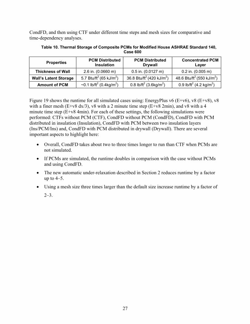
Figure 19 shows the runtime for all simulated cases using: EnergyPlus v6 (E+v6), v8 (E+v8), v8 with a finer mesh (E+v8 dx/3), v8 with a 2 minute time step (E+v8 2min), and v8 with a 4 minute time step (E+v8 4min). For each of these settings, the following simulations were performed: CTFs without PCM (CTF), CondFD without PCM (CondFD), CondFD with PCM distributed in insulation (Insulation), CondFD with PCM between two insulation layers (Ins/PCM/Ins) and, CondFD with PCM distributed in drywall (Drywall). There are several important aspects to highlight here:
• Overall, CondFD takes about two to three times longer to run than CTF when PCMs are not simulated.
• If PCMs are simulated, the runtime doubles in comparison with the case without PCMs and using CondFD.
• The new automatic under-relaxation described in Section 2 reduces runtime by a factor up to 4–5.
• Using a mesh size three times larger than the default size increase runtime by a factor of
2–3.
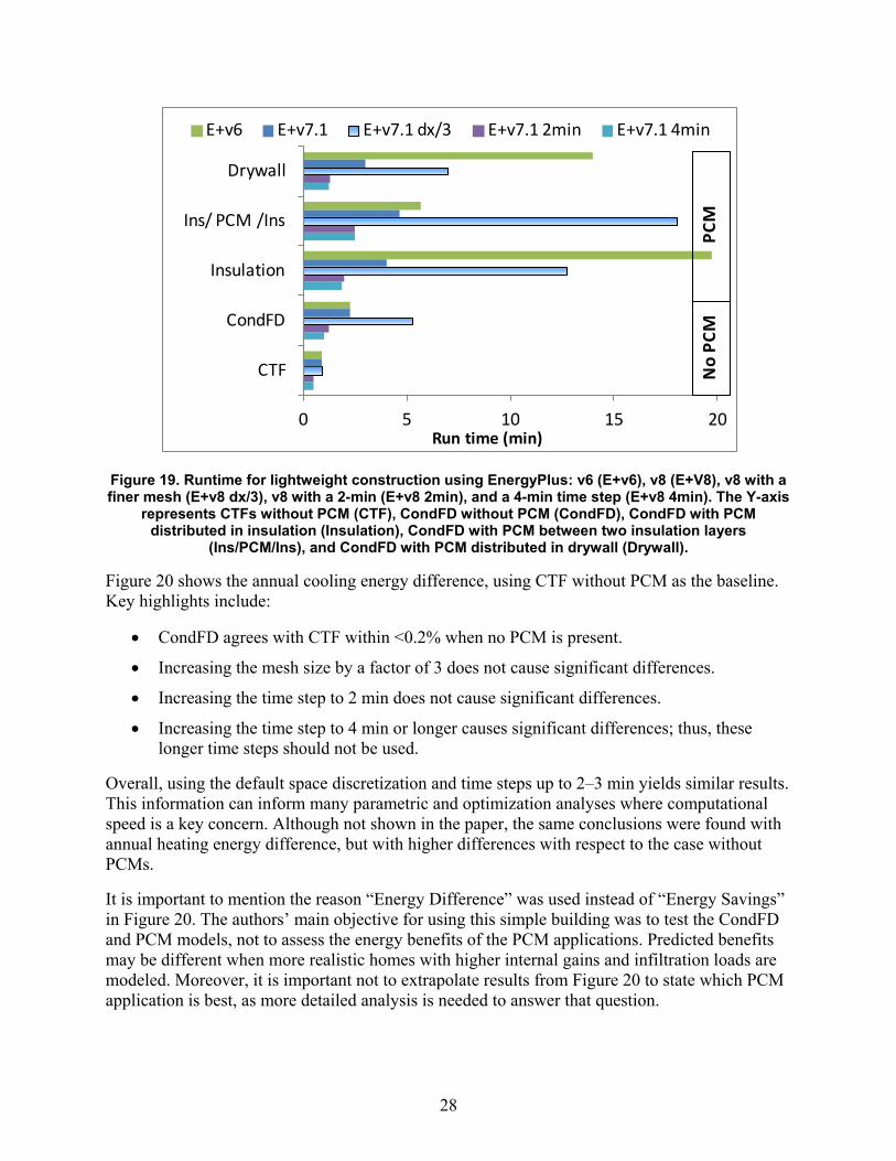
28
Figure 19. Runtime for lightweight construction using EnergyPlus: v6 (E+v6), v8 (E+V8), v8 with a finer mesh (E+v8 dx/3), v8 with a 2-min (E+v8 2min), and a 4-min time step (E+v8 4min). The Y-axis
represents CTFs without PCM (CTF), CondFD without PCM (CondFD), CondFD with PCM distributed in insulation (Insulation), CondFD with PCM between two insulation layers
(Ins/PCM/Ins), and CondFD with PCM distributed in drywall (Drywall).
Figure 20 shows the annual cooling energy difference, using CTF without PCM as the baseline. Key highlights include:
• CondFD agrees with CTF within <0.2% when no PCM is present.
• Increasing the mesh size by a factor of 3 does not cause significant differences.
• Increasing the time step to 2 min does not cause significant differences.
• Increasing the time step to 4 min or longer causes significant differences; thus, these longer time steps should not be used.
Overall, using the default space discretization and time steps up to 2–3 min yields similar results. This information can inform many parametric and optimization analyses where computational speed is a key concern. Although not shown in the paper, the same conclusions were found with annual heating energy difference, but with higher differences with respect to the case without PCMs.
It is important to mention the reason “Energy Difference” was used instead of “Energy Savings” in Figure 20. The authors’ main objective for using this simple building was to test the CondFD and PCM models, not to assess the energy benefits of the PCM applications. Predicted benefits may be different when more realistic homes with higher internal gains and infiltration loads are modeled. Moreover, it is important not to extrapolate results from Figure 20 to state which PCM application is best, as more detailed analysis is needed to answer that question.
0 5 10 15 20
CTF
CondFD
Insulation
Ins/ PCM /Ins
Drywall
Run time (min)
E+v6 E+v7.1 E+v7.1 dx/3 E+v7.1 2min E+v7.1 4min
No
PCM
PCM

29
Figure 20. Model evaluation results for annual cooling energy difference using legends as in Figure 19
3.4.2 PCM Model Evaluation Using BEopt New House A second house was analyzed in EnergyPlus using the same weather data. This is a two-story, slab-on-grade, 231-m2 (2500-ft2) house with three bedrooms, two bathrooms, an unconditioned attic, garage and a more realistic HVAC system. A few modifications were made to the original EnergyPlus model generated by BEopt to accommodate PCMs:
• The house was created in BEopt and the input EnergyPlus file (idf) was exported to EnergyPlus, where PCMs were introduced.
• The properties of the insulation used in the walls and attic were modified to the properties for PCM-distributed insulation shown in Table 9.
• The walls and attic were assumed to be studless and trussless to simplify the problem as a first approximation.
These assumptions resulted in a well-insulated building envelope, as the equivalent R-values of the studless wall and trussless attic are RSI-2.7 (RIP-15.3) and RSI-6.7 (RIP-40), respectively. Thus, this case represents a home having walls with an R-value close to a wall assembly consisting of RIP-19 batts, 5 × 15 cm (2 × 6 in.) studs, 60 cm (24 in.) apart from center having a RSI-2.9 (RIP-16.3). In contrast a typical wall consisting of RIP-13 batts, 5 × 10 cm (2 × 4 in.) studs, 40 cm (16 in.) apart from center have a RSI-2 (RIP-11.4).
Table 11 shows storage capacity for the PCM assemblies in the walls using PCM composite properties shown in Table 9. As with the ASHRAE-modified Case 600, the PCM distributed in insulation has the lowest storage capacity because the insulation is low density. Higher latent storage values could be achieved by increasing the percentage of PCM or the thickness of insulation layer.
-4% 1% 6% 11%
CTF
CondFD
Insulation
Ins/ PCM/ Ins
Drywall
Cooling Energy Difference (%)
E+v6 E+v7.1 E+v7.1 dx/3 E+v7.1 2min E+v7.1 4min
PCM
No
PCM

30
Table 11. Thermal Storage of Composite PCMs for BEopt New House
Properties PCM
Distributed Insulation
PCM Distributed Drywall
Concentrated PCM Layer
Thickness of Wall 3.5 in. (0.089 m) 0.5in. (0.0127 m) 0.2in. (0.005 m) Wall’s Latent Storage 7.7 Btu/ft2 (87 kJ/m2) 36.8 Btu/ft2 (420 kJ/m2) 48.6 Btu/ft2 (550 kJ/m2)
Amount of PCM 0.1 lb/ft2 (0.5 kg/m2) 0.8 lb/ft2 (3.8kg/m2) 0.9 lb/ft2 (4.2kg/m2)
Figure 21 shows the predicted monthly cooling electric energy reduction for the following PCM applications: upper half of the attic insulation enhanced with PCM (Upper Attic), lower half of the attic insulation enhanced with PCM (Lower Attic), PCM concentrated at the middle of the attic insulation (AtticRCR), wall cavity with PCM distributed in insulation, PCM concentrated at the middle of the wall cavity insulation (WallRCR), PCM distributed in the ceiling and wall drywall (Drywall) and combination of WallRCR with PCM distributed in Drywall (WallRCR-DW). The last PCM application was chosen to evaluate the PCM model’s ability to simulate walls with different PCMs in a single wall. The predicted annual electric cooling consumption for the house without PCM was 5,500 kWh, less than half the 2009 average for homes in Arizona, which is 12,900 (EIA 2011). In all cases, the EnergyPlus runtime was about 20 min using a 2-min time step, about twice as long as CTF. This suggests that the CondFD and PCM models are working properly, as previously shown with the modified ASHRAE Standard 140 building. Moreover, no instability problems were detected.
Figure 21. Model evaluation results for monthly cooling electric energy difference for BEopt house using melting ranges specified in Table 9 for Phoenix, Arizona: upper half (Upper Attic) and lower
half (Lower Attic) of the attic insulation with PCM, PCM concentrated at the middle of the attic insulation (RCRAttic), wall cavity with PCM distributed in insulation (Walls), PCM concentrated at
the middle of the wall cavity insulation (RCRWall), PCM distributed drywall (Drywall) and combination of RCRWall and PCM-Drywall (RCRWall-DW)
0.0%
0.1%
0.2%
0.3%
0.4%
0.5%
0.6%
0.7%
0.8%
Mar Apr May Jun Jul Aug Sep Oct Nov
Diffe
renc
e (%
)
Upper Attic Lower Attic RCRAttic Walls RCRWall Drywall RCRWall_DW
31
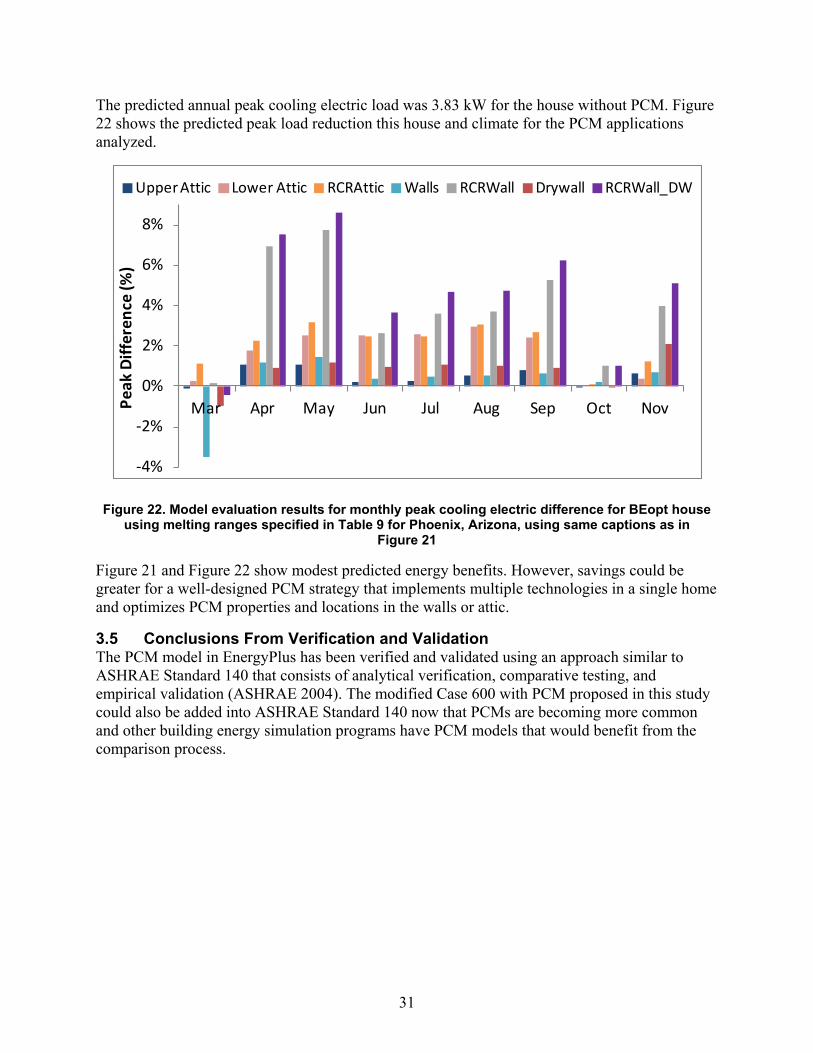
The predicted annual peak cooling electric load was 3.83 kW for the house without PCM. Figure 22 shows the predicted peak load reduction this house and climate for the PCM applications analyzed.
Figure 22. Model evaluation results for monthly peak cooling electric difference for BEopt house using melting ranges specified in Table 9 for Phoenix, Arizona, using same captions as in
Figure 21
Figure 21 and Figure 22 show modest predicted energy benefits. However, savings could be greater for a well-designed PCM strategy that implements multiple technologies in a single home and optimizes PCM properties and locations in the walls or attic.
3.5 Conclusions From Verification and Validation The PCM model in EnergyPlus has been verified and validated using an approach similar to ASHRAE Standard 140 that consists of analytical verification, comparative testing, and empirical validation (ASHRAE 2004). The modified Case 600 with PCM proposed in this study could also be added into ASHRAE Standard 140 now that PCMs are becoming more common and other building energy simulation programs have PCM models that would benefit from the comparison process.
-4%
-2%
0%
2%
4%
6%
8%
Mar Apr May Jun Jul Aug Sep Oct NovPeak
Diff
eren
ce (%
)
Upper Attic Lower Attic RCRAttic Walls RCRWall Drywall RCRWall_DW

32
4 Detailed Diagnostics Available for Whole Building Analysis for Phase Change Material Systems Using Verified Phase Change Material Model
Once the CondFD and PCM algorithms were validated, the same BEopt new house described in Section 3.4.2 was analyzed in more detail in EnergyPlus for the Phoenix location for several PCM applications in walls. The intent is to show how the whole-building analysis of a PCM system can produce information that is useful for selecting the type, amount, and location of PCMs for improved energy performance (Tabares-Velasco et al. 2012). However, it is not the purpose of this study to perform a parametric analysis of PCMs or predict actual energy savings from PCMs. Table 9 shows the properties of the PCM aggregate materials in walls analyzed in this study: PCM distributed in insulation, PCM distributed in drywall, and concentrated PCM layer. From these three materials, concentrated PCM has the most storage capacity, as it is the only concentrated application analyzed in this study.
Figure 23 shows predicted monthly cooling electric energy reduction for the analyzed PCM applications. All monthly savings were divided by the annual energy use for the building without PCMs. The PCM applications analyzed are: PCM distributed in drywall on the ceiling (DW_Ceil) and walls (DW_Walls), PCM distributed in wall insulation (Walls), PCM concentrated at the middle of the wall cavity insulation (RCRWall) and a combination of RCRWall with PCM distributed in Drywall (RCRWall-DW). The last application was selected to further investigate possible combinations of different PCMs. It illustrates potential savings when multiple PCM applications are used within a single building. For this particular case, the combination of RCRWall with PCM distributed in Drywall (RCRWall-DW) achieved an annual percentage savings of around 4% or approximately 210 kWh. However, more in-depth parametric analysis is needed before any conclusions can be made. This study did not analyze different melting temperatures or storage capacities to optimize energy and/or peak load savings.
Figure 23. Predicted cooling energy savings for multiple PCM strategies for a BEopt house in Phoenix
0.0%
0.1%
0.2%
0.3%
0.4%
0.5%
0.6%
0.7%
0.8%
Mar Apr May Jun Jul Aug Sep Oct Nov
Mon
thly
Sav
ings
(%
of a
nnua
l ene
rgy
use)
DW_Ceil Walls RCRWall Drywall DW_Walls RCRWall_DW
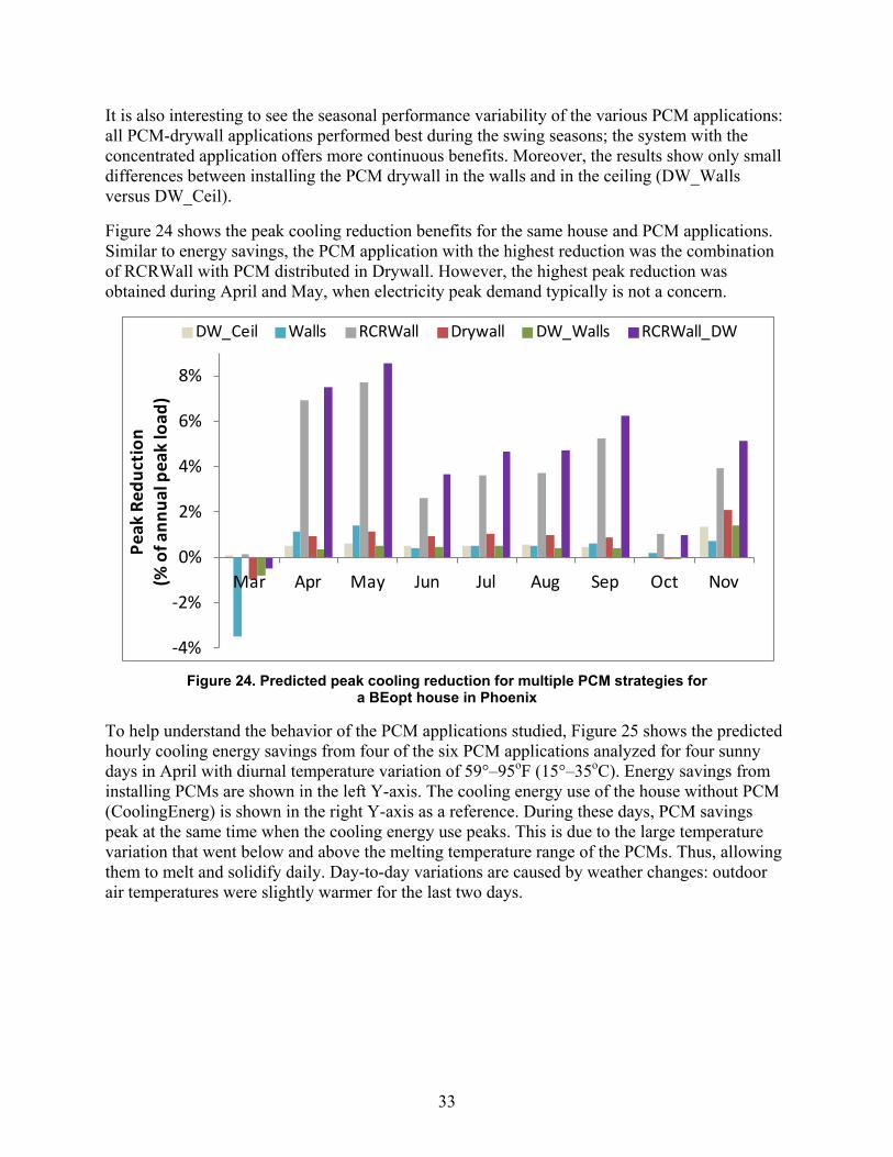
33
It is also interesting to see the seasonal performance variability of the various PCM applications: all PCM-drywall applications performed best during the swing seasons; the system with the concentrated application offers more continuous benefits. Moreover, the results show only small differences between installing the PCM drywall in the walls and in the ceiling (DW_Walls versus DW_Ceil).
Figure 24 shows the peak cooling reduction benefits for the same house and PCM applications. Similar to energy savings, the PCM application with the highest reduction was the combination of RCRWall with PCM distributed in Drywall. However, the highest peak reduction was obtained during April and May, when electricity peak demand typically is not a concern.
Figure 24. Predicted peak cooling reduction for multiple PCM strategies for a BEopt house in Phoenix
To help understand the behavior of the PCM applications studied, Figure 25 shows the predicted hourly cooling energy savings from four of the six PCM applications analyzed for four sunny days in April with diurnal temperature variation of 59°–95oF (15°–35oC). Energy savings from installing PCMs are shown in the left Y-axis. The cooling energy use of the house without PCM (CoolingEnerg) is shown in the right Y-axis as a reference. During these days, PCM savings peak at the same time when the cooling energy use peaks. This is due to the large temperature variation that went below and above the melting temperature range of the PCMs. Thus, allowing them to melt and solidify daily. Day-to-day variations are caused by weather changes: outdoor air temperatures were slightly warmer for the last two days.
-4%
-2%
0%
2%
4%
6%
8%
Mar Apr May Jun Jul Aug Sep Oct Nov
Peak
Red
uctio
n (%
of a
nnua
l pea
k lo
ad)
DW_Ceil Walls RCRWall Drywall DW_Walls RCRWall_DW
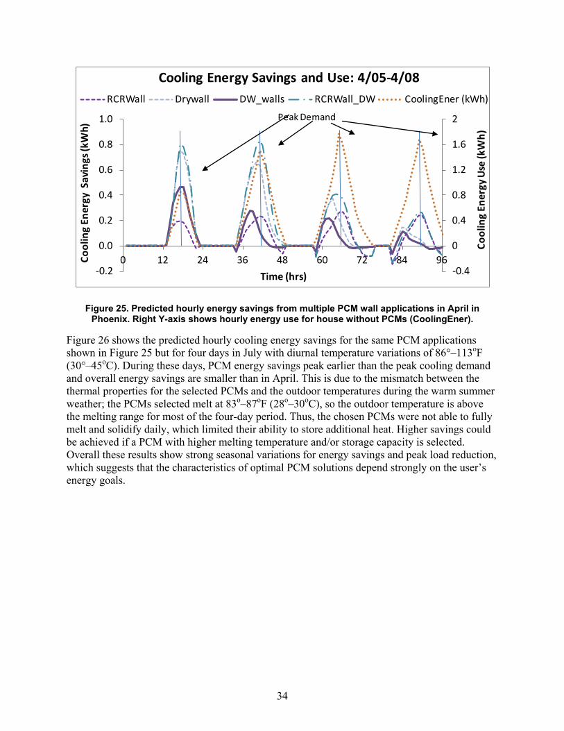
34
Figure 25. Predicted hourly energy savings from multiple PCM wall applications in April in Phoenix. Right Y-axis shows hourly energy use for house without PCMs (CoolingEner).
Figure 26 shows the predicted hourly cooling energy savings for the same PCM applications shown in Figure 25 but for four days in July with diurnal temperature variations of 86°–113oF (30°–45oC). During these days, PCM energy savings peak earlier than the peak cooling demand and overall energy savings are smaller than in April. This is due to the mismatch between the thermal properties for the selected PCMs and the outdoor temperatures during the warm summer weather; the PCMs selected melt at 83o–87oF (28o–30oC), so the outdoor temperature is above the melting range for most of the four-day period. Thus, the chosen PCMs were not able to fully melt and solidify daily, which limited their ability to store additional heat. Higher savings could be achieved if a PCM with higher melting temperature and/or storage capacity is selected. Overall these results show strong seasonal variations for energy savings and peak load reduction, which suggests that the characteristics of optimal PCM solutions depend strongly on the user’s energy goals.
-0.4
0
0.4
0.8
1.2
1.6
2
-0.2
0.0
0.2
0.4
0.6
0.8
1.0
0 12 24 36 48 60 72 84 96
Cool
ing
Ener
gy U
se (k
Wh)
Cool
ing
Ener
gy S
avin
gs (k
Wh)
Time (hrs)
Cooling Energy Savings and Use: 4/05-4/08RCRWall Drywall DW_walls RCRWall_DW CoolingEner (kWh)
Peak Demand
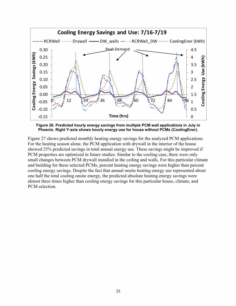
35
Figure 26. Predicted hourly energy savings from multiple PCM wall applications in July in Phoenix. Right Y-axis shows hourly energy use for house without PCMs (CoolingEner).
Figure 27 shows predicted monthly heating energy savings for the analyzed PCM applications. For the heating season alone, the PCM application with drywall in the interior of the house showed 25% predicted savings in total annual energy use. These savings might be improved if PCM properties are optimized in future studies. Similar to the cooling case, there were only small changes between PCM drywall installed in the ceiling and walls. For this particular climate and building for these selected PCMs, percent heating energy savings were higher than percent cooling energy savings. Despite the fact that annual onsite heating energy use represented about one half the total cooling onsite energy, the predicted absolute heating energy savings were almost three times higher than cooling energy savings for this particular house, climate, and PCM selection.
0
0.5
1
1.5
2
2.5
3
3.5
4
4.5
-0.15
-0.10
-0.05
0.00
0.05
0.10
0.15
0.20
0.25
0.30
0 12 24 36 48 60 72 84 96
Cool
ing
Ener
gy U
se (k
Wh)
Cool
ing
Ener
gy S
avin
gs (k
Wh)
Time (hrs)
Cooling Energy Savings and Use: 7/16-7/19RCRWall Drywall DW_walls RCRWall_DW CoolingEner (kWh)
Peak Demand

36
Figure 27. Predicted heating energy savings from different PCM strategies
0%
1%
2%
3%
4%
5%
6%
7%
8%
Jan Feb Mar Apr Nov Dec
Enen
rgy
Savi
ngs
(% o
f ann
ual e
nerg
y us
e)
DW_Ceil Walls RCRWall Drywall_All DW_Walls RCRWall-DW
37
5 Conclusions This report summarizes the approach used to validate the CondFD and PCM algorithms in EnergyPlus. During this process, more than 10 programming bugs were identified and fixed in the PCM model. Version 7.1 of EnergyPlus will include the validated PCM model and fixes, which speed up the runtime and allow for simulation of PCMs with variable thermal conductivity.
This study also identified a few key limitations and guidelines when using the EnergyPlus PCM model:
• Time steps ≤3 min should be used; the selected value for the Fourier number can have an important influence on the analysis.
• Accuracy issues can arise when modeling PCMs with strong hysteresis. Users may want to parametrically vary the enthalpy curves to estimate the impact of the single-curve limitation when modeling a material with such behavior.
• The default CondFD node spacing values can be used with acceptable monthly and annual results. However, if sub-hourly performance and analysis is required, users should use node spacing values about one third of the default size (equal to using a Space Discretization Constant in EnergyPlus of about 0.3–0.5)
This study also shows how the whole-building analysis of a PCM system can produce information that is useful for selecting the type, amount, and location of PCMs for improved energy performance. This application of whole-building analysis is demonstrated for three residential building envelope technologies containing specific PCMs: PCM distributed in insulation, PCM distributed in drywall and concentrated PCM layer between insulation in the walls. These technologies are compared based on peak reduction and energy savings using the CondFD algorithm in EnergyPlus. Preliminary results suggest that considerable annual energy savings could be achieved using PCMs in residential buildings, but that careful design is needed to optimize PCM solutions according to the specific user goals for peak demand and energy use reductions. Future research will include more detailed parametric analyses to optimize PCM wall strategies.

38
References 1. Ahmad, M., A. Bontemps, H. Sallée and D. Quenard. (2006). "Experimental investigation and
computer simulation of thermal behavior of wallboards containing a phase change material." Energy and Buildings 38(4): 357-366.
2. ASHRAE (2004). ANSI/ASHRAE Standard 140-2004. "Standard Method of Test for the Evaluation of Building Energy Analysis Computer Programs." Atlanta, GA, ASHRAE: 151.
3. Athienitis, A. K., C. Liu, D. Hawes, D. Banu, D. Feldman. (1997). "Investigation of the thermal performance of a passive solar test-room with wall latent heat storage." Building and Environment 32(5): 405-410.
4. Cao, S., A. Gustavsen, S. Uvsløkk, B.P. Jelle, J. Gilbert, J. Maunuksela . (2010). "The Effect of Wall-Integrated Phase Change Material Panelson the Indoor Air and Wall Temperature – Hot box Experiments." Zero Emission Buildings,- Proceedings of Renewable Energy Conference 2010, Trondheim, Norway: 15-26.
5. Carslaw, H. S. and J. C. Jaeger (1959). Conduction of Heat in Solids, Oxford University Press.
6. Casey, S. and C. Booten. (2011). Energy Savings Measure Packages: New Homes. Golden, National Renewable Energy Laboratory: 205.
7. Childs, K.W. (2005). Heating 7.2 User's Manual, Oak Ridge National Laboratory: 242.
8. Childs, K. and T. Stovall. (2012). Use of phase change material in a wall assembly: a case study of technical potential in two climates, ORNL TM-34268, March 2012.
9. Drake, J.B. (1987). A study of the optimal transition temperature of PCM wallboard for solar energy storage, Oak Ridge National Laboratory. ORNL\TM -10210.
10. EIA. (2011). 2009 Residential Energy Consumption Survey. Retrieved 10/21/2011, 2011, from http://205.254.135.24/consumption/residential/index.cfm.
11. Haavi, T., A. Gustavsen, S. Cao, S. Uvsløkk S and B.P. Jelle. (2011). "Numerical Simulations of a Well-Insulated Wall Assembly with Integrated Phase Change Material Panels - Comparison with Hot Box Experiments," The International Conference on Sustainable Systems and the Environment, Sharjah, Sharjah, United Arab Emirates
12. Halford, C. K. and R.F. Boehm. (2007). "Modeling of phase change material peak load shifting." Energy and Buildings 39(3): 298-305.
13. Heim, D. (2010). "Isothermal storage of solar energy in building construction." Renewable Energy 35(4): 788-796.
14. Heim, D. and J. A. Clarke. (2004). "Numerical modelling and thermal simulation of PCM-gypsum composites with ESP-r." Energy and Buildings 36(8): 795-805.
15. Hensen, J.L.M. and A. Nakhi. (1994). "Fourier and Biot numbers and the accuracy of conduction modelling." BEP '94 Conference "Facing the Future", York, Building Environmental Performance Analysis Club (BEPAC).
16. Ibáñez, M., A. Lázaro, B. Zalba, L.F. Cabeza. (2005). "An approach to the simulation of PCMs in building applications using TRNSYS." Applied Thermal Engineering 25(11-12): 1796-1807.
39
17. Kedl, R.J. (1990). "Conventional wallboard with latent heat storage for passive solar applications." 25th Intersociety Energy Conversion Engineering Conference, Reno, NV, 12-17 Aug. 1990
18. Khudhair, A.M. and M.M. Farid (2004). "A review on energy conservation in building applications with thermal storage by latent heat using phase change materials." Energy Conversion and Management 45(2): 263-275.
19. Kosny, J., S. Shrestha, D. Yarbrough, P. Childs, W. Miller, M. Bianchi, J. Smith,… E. Lee. (2010a). "Theoretical and experimental thermal performance analysis of building shell components containing blown fiberglass insulation enhanced with phase-change materials (PCM)." Thermal Performance of the Exterior Envelopes of Whole Buidings XI International Conference, Clearwater Beach, Florida: 13.
20. Kosny, J., S. Shrestha, T. Stovall and D. Yarbrough. (2010b). "Theoretical and experimental thermal performance analysis of complex thermal storage membrane containing bio-base phase change material (PCM)." Thermal Performance of The Exterior Envelopes of Whole Buidings XI International Conference, Clearwater Beach, Florida: 11.
21. Koschenz, M. and B. Lehmann (2004). "Development of a thermally activated ceiling panel with PCM for application in lightweight and retrofitted buildings." Energy and Buildings 36(6): 567-578.
22. Kuznik, F. and J. Virgone. (2009). "Experimental investigation of wallboard containing phase change material: Data for validation of numerical modeling." Energy and Buildings 41(5): 561-570.
23. Kuznik, F., J. Virgone, and K. Johannes. (2010). "Development and validation of a new TRNSYS type for the simulation of external building walls containing PCM." Energy and Buildings 42(7): 1004-1009.
24. Kuznik, F., J. Virgone, J.R. Roux. (2008). "Energetic efficiency of room wall containing PCM wallboard: A full-scale experimental investigation." Energy and Buildings 40(2): 148-156.
25. Pasupathy, A., R. Velraj, R.V. Seeniraj. (2008). "Phase change material-based building architecture for thermal management in residential and commercial establishments." Renewable and Sustainable Energy Reviews 12(1): 39-64.
26. Pedersen, C.O. (2007). "Advanced zone simulation in EnergyPlus: incorporation of variable properties and phase change material (PCM) capability." Building Simulation 2007, Beijing, China.
27. Petrie, T.W., P.W. Childs, J.E. Christian, K.W. Childs, D.J. Shramo. (1997). "Thermal behavior of mixtures of perlite and phase change material in simulated climate." Insulation Materials: Testing and Applications 3, ASTM STP 1320, Quebec City, USA, ASTM.
28. Polly, B., M. Gestwick, M. Bianchi, R. Anderson, S. Horowitz, C. Christensen, and R Judkoff. (2011). A method for determining optimal residential energy efficiency retrofit packages. NREL Technical Report DOE/GO-102011-3261. Golden, CO, National Renewable Energy Laboratory: 79

40
29. Schossig, P., H. M. Henning, S. Gschwandera and T. Haussmann. (2005). "Micro-encapsulated phase-change materials integrated into construction materials." Solar Energy Materials and Solar Cells 89(2-3): 297-306.
30. Sharma, A., V.V. Tyagi, C.R. Chen and D. Buddhi. (2009). "Review on thermal energy storage with phase change materials and applications." Renewable and Sustainable Energy Reviews 13(2): 318-345.
31. Solomon, A. D. (1979). "Design criteria in PCM wall thermal storage." Energy 4(4): 701-709.
32. Stovall, T. K. and J. J. Tomlinson (1995). "What are the potential benefits of including latent storage in common wallboard?" Journal of Solar Energy Engineering, Transactions of the ASME 117(4): 318-325.
33. Tabares-Velasco, P.C., C. Christensen, and M. Bianchi (2012). "Validation methodology to allow simulated peak reduction and energy performance analysis of residential building envelope with phase change materials." ASHRAE Transactions, SA-12-C012: 8 pages.
34. Tabares-Velasco, P. C., C. Christensen, and M. Bianchi (2012). "Verification and Validation of EnergyPlus Phase Change Material Model for Opaque Wall Assemblies." Building and Environment 54: 186-196.
35. Tabares-Velasco, P. C. and B. Griffith. (2011). " Diagnostic test cases for verifying surface heat transfer algorithms and boundary conditions in building energy simulation programs," Journal of Building Performance Simulation, doi:10.1080/19401493.2011.595501
36. Tomlinson, J. J. and D. D. Heberle. (1990). "Analysis of wallboard containing a phase change material," 25th Intersociety Energy Conversion Engineering Conference, Reno, NV, 12-17 Aug. 1990.
37. Tyagi, V.V. and D. Buddhi. (2007). "PCM thermal storage in buildings: a state of art." Renewable and Sustainable Energy Reviews 11(6): 1146-1166.
38. Virgone, J., J. Noël and R. Reisdorf. (2009). Numerical study of the influence of the thickness and melting point on the effectiveness of phase change materials: application to the renovation of a low inertia school. Eleventh International IBPSA Conference. Glasgow, Scotland, July 27-30, 2009: 408-413
39. Wang, X., Y. Zhang, W. Xiao, R.L. Zeng, Q.L. Zhang and H.F. Di. (2009). "Review on thermal performance of phase change energy storage building envelope." Chinese Science Bulletin 54(6): 920-928.
40. Waters, J.R. and A.J. Wright (1985). "Criteria for the distribution of nodes in multilayer walls in finite-difference thermal modelling." Building and Environment 20(3): 151-162.
41. Zhu, N., Z. Ma and S. Wang (2009). "Dynamic characteristics and energy performance of buildings using phase change materials: A review." Energy Conversion and Management 50(12): 3169-3181.

41
Appendix A. Phase Change Material Properties Used in Experimental Validation Thickness: 0.0053 m
Thermal conductivity: Solid (T <21.6°C): 0.18 W/mK
Liquid (T>21.6°C): 0.14 W/mK
Density: 855 kg/m3
Specific Heat: 2500 J/kg-K
Enthalpy Versus Temperature Data for DuPont Energain PCM used in Experimental Validation
T (oC)
H (J/kg oC)
T (oC)
H (J/kg oC)
–9.0 0.001 12.5 81,010
–7.0 5,200 15.0 93,760
–5.0 10,800 17.5 109,385
–4.0 13,750 20.0 129,635
–3.0 16,850 22.5 157,385
–2.0 20,350 23.5 170,985
–1.0 24,750 24.0 177,535
–0.2 30,030 25.0 186,185
0.0 31,610 26.0 191,185
1.0 37,160 27.0 195,535
2.0 40,510 28.0 199,485
2.5 42,160 29.0 203,135
4.0 47,335 30.0 206,335
5.0 50,885 31.5 210,535
7.5 60,135 45.0 244,960
10.0 70,010 80.0 332,460

42
Appendix B. EnergyPlus Conduction Finite Difference and Phase Change Material Algorithms EnergyPlus is building energy simulation software that uses the zone heat balance model to predict thermal loads and zone air conditions. Conduction heat transfer processes are an important element of this model that connect all the interactions between the inside and outside surfaces. EnergyPlus was originally developed using CTFs to calculate conduction processes throughout walls, windows and floors. CTFs are very powerful as they relate the current surface heat flux and temperature values to previous surface heat flux and temperature values (ASHRAE 2009). Thus, with CTFs there is no need to calculate temperatures within the surface, which reduces computational requirements for the simulation. The main disadvantages of CTFs are that they assume constant thermal properties and provide no information about internal processes in a wall. Therefore, the EnergyPlus developers added an implicit CondFD model to EnergyPlus, as shown in Figure B.1.
Figure B.1. EnergyPlus heat transfer algorithms
The CondFD model in EnergyPlus has the following four types of nodes, as shown in Figure B.2: (1) interior surface nodes; (2) interior nodes; (3) material interface nodes; and (4) external surface nodes (EnergyPlus 2010). The grid for each material is established by specifying a half node for each edge of a material and equal size nodes for the rest of the material.
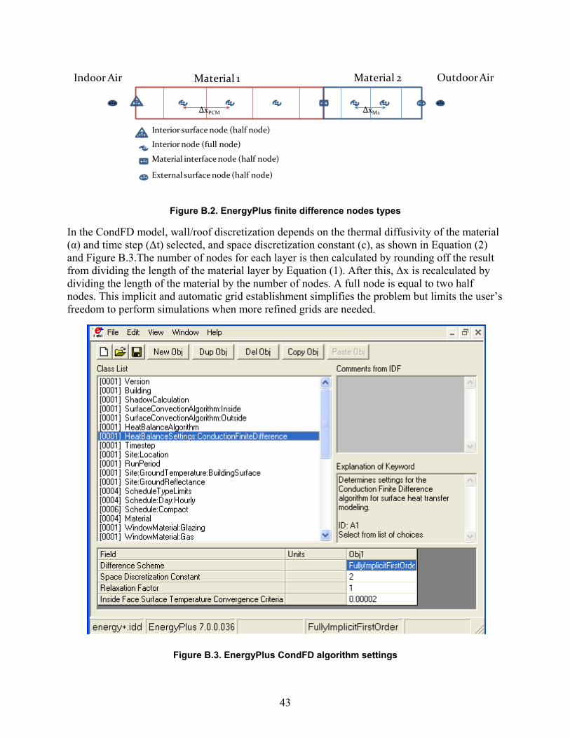
43
Figure B.2. EnergyPlus finite difference nodes types
In the CondFD model, wall/roof discretization depends on the thermal diffusivity of the material (α) and time step (Δt) selected, and space discretization constant (c), as shown in Equation (2) and Figure B.3.The number of nodes for each layer is then calculated by rounding off the result from dividing the length of the material layer by Equation (1). After this, Δx is recalculated by dividing the length of the material by the number of nodes. A full node is equal to two half nodes. This implicit and automatic grid establishment simplifies the problem but limits the user’s freedom to perform simulations when more refined grids are needed.
Figure B.3. EnergyPlus CondFD algorithm settings
Indoor Air Material 1 Material 2
ΔxPCM ΔxM2
Outdoor Air
External surface node (half node)
Material interface node (half node)
Interior node (full node)
Interior surface node (half node)

44
For the PCM algorithm, the CondFD method is coupled with an enthalpy-temperature function (see Equation 3) that the user inputs to account for enthalpy changes during phase change (Pedersen 2007). As an example, the data for the PCM shown in Appendix A are shown in Figure B.4. The enthalpy-temperature function is used to develop an equivalent specific heat at each time step: each temperature-enthalpy data pair is input for the range of temperature analyzed. The “Temperature Coefficient for Thermal Conductivity” is set to zero in Figure B.4, but it could be modified if the PCM thermal conductivity shows linear behavior. For this case, the variable thermal conductivity was input as a stepwise function (see Figure B.5). All these features were fixed and validated in this study.

45
Figure B.4. EnergyPlus PCM input model

46
Figure B.5. EnergyPlus input for material with variable thermal conductivity