Embed Size (px)
Citation preview
UNIVERSITY OF LEOBEN
DEPARTMENT OF PETROLEUM ENGINEERING
CHAIR FOR DRILLING AND COMPLETION ENGINEERING
VERIFICATION AND COMPARISON OF THE
METHODS WHICH USE LOG DATA TO ESTIMATE
ROCK PROPERTIES AND INFLUENCE OF ROCK
PROPERTIES ON DRILLING DYNAMICS AND BHA
DESIGN
MASTER’s THESIS
Author:
Žiga Škrjanc, MSc
Supervisor:
Gerhard Thonhauser, Univ.-Prof. Dipl.-Ing. Dr.mont.
Leoben, 2016


PROOF SHEET FOR MSc THESIS SUBMISSION
Name of graduate student: Žiga Škrjanc
Matriculation number: 1435116
Title of the MSc Thesis: Verification and Comparison of the Methods
which Use Log Data to Estimate Rock Properties and Influence of Rock Properties on
Drilling Dynamics and BHA Design
THE MSc THESIS HAS BEEN SUBMITTED ON ………………, ………. .
…………..………………………………………………….. Administration of Montanuniversität Leoben, Main Library
Montanuniversität Leoben, Austria


EIDESSTATTLICHE ERKLÄRUNG
“Ich erkläre an Eides statt, dass ich die vorliegende Diplomarbeit selbständig und ohne fremde Hilfe verfasst, andere als die angegebenen Quellen und Hilfsmittel nicht benutzt und
die den benutzten Quellen wörtlich und inhaltlich entnommenen Stellen als solche erkenntlich gemacht habe.“
AFFIDAVIT
“I hereby declare that the content of this work is my own composition and has not been
submitted previously for any higher degree. All extracts have been distinguished using quoted
references and all information sources have been acknowledged.”
Leoben, ________, 2016
…………………………………….. Signature of Graduate Student
Žiga Škrjanc


Acknowledgment
I would like to thank Dipl.-Ing. Dr.mont.Gerhard Pittino, who kindly organized and carried
out the UCS tests.


DEDICATION
I dedicate this thesis to my parents who supported me throughout the study.


I
Kurzfassung
Heutzutage sind Öl- und Gasvorkommen an herausfordernden Orten und in Tiefen, die man
vor nur wenigen Jahrzenten gar nicht erreichen konnte. Um diese Lagerstätten zu erreichen, ist modernste Technologie und Know-How erforderlich. Geomechanische Fragen sind nur ein
Teil der Herausforderungen bei Bohrungen. Die Auswertung der In-situ-
Gesteinseigenschaften ist ein wichtiger Bestandteil der geomechanischen Analyse und es hilft,
Prinzipien wie Bohrlochstabilität, Bohrmeißelauswahl, BHA Design, Lochqualität, Steckenbleiben und Bohrungsdynamik. Bohrungsdynamik ist ein weiterer nicht gut
durchdrungener Aspekt, der Kosten, NPT und die Zahl der Ausfälle wesentlich erhöhen kann. All dieses Wissen ist entscheidend für eine erfolgreiche Bohrung von gerichteten, stark abgelenkten und horizontalen Bohrlöchern.
Die Arbeit konzentriert sich auf die Modellierung der In-Situ Gesteinsfestigkeit mithilfe
akustischer, Dichte- oder anderer Messungen. Für die Arbeit wurden Sandstein- und
Kalksteinproben genommen. Aus ihnen wurden Zylinder mit 5 Centimeter Durchmesser
gebohrt. Die primäre Wellengeschwindigkeit wurde gemessen und ein UCS-Test (einaxiale
Druckfestigkeit) wurde für beide Proben durchgeführt . Als Ergebnis wird der Erfassungsprozess und die empfohlene Verwendung beschrieben.
Bohrungsdynamik kann zu Störungen wie Reibschwingung, niedrige oder hohe Torsionsschwingung, Meißelwirbel oder zufällige Torsionsschwingung führen. Alle diese sind vom BHA Design, Paramatern der Oberflächenbohrung und den Gesteinseigenschaften abhängig. Alle diese Erscheinungen werden in der Arbeit untersucht und als Ergebnis
Empfehlungen und beste Bohrpraktiken gegeben.
II
Abstract
At this present time, oil and gas reservoirs are found in challenging locations and can be
reached at depths which were impossible to achieve a few decades ago. In order to reach these
reservoirs, both state of the art technology and a great knowledge are required.
Geomechanical problems are just one issue which may occur during drilling operations. In
situ rock properties evaluation is an important element of geomechanical analysis, which
helps in understanding principles such as wellbore stability, bit selection, BHA design, hole
quality, stuck pipe studies and drilling dynamics. Drilling dynamics is another phenomenon,
which is not well understood and can substantially increase costs, Non-Productive Time
("NPT") and failures. All this knowledge is crucial for the successful drilling of directional,
highly deviated and horizontal wells.
This thesis focuses on rock strength modelling with the use of logs to enable an estimation of
in situ rock properties from sonic, density or another log. Sandstone and limestone rock
samples were acquired for this thesis, which were subsequently cored into five centimetre
cylinders. Primary wave velocity was measured and a Uniaxial Compressive Strength
("UCS") test was carried out on both samples. As a result, the acquiring process is given and
recommended usage described.
Drilling dynamics can lead to dysfunctions, such as full stick slip, low or high torsional
oscillation, bit whirl or random torsional oscillation. All of these are dependent on BHA
design, surface drilling parameters and rock properties. All of these phenomena are
investigated in this thesis and, as a result, recommendations and best drilling practices are
given.
III
List of Tables
Table 1: Typical values of critical porosity. (Mavko et al., 1998) ........................................ 8
Table 2: Some relations between elastic moduli. (Fjaer et al., 2008 ) ................................ 12
Table 3 Typical bulk modulus values for the most common materials. ............................ 13
Table 4: Polynomial relations of velocity-density dependance as presented by
Castagna et al. (1993). Units are km/s and g/cc for velocity and density,
respectively. (Mavko et al., 1998) ........................................................................ 26
Table 5: The case studies summary. ................................................................................... 47
Table 6: Mineral composition of the sample sandstone. ..................................................... 53
Table 7: The tests that were done on the sandstone formation from where the sample
was taken. ............................................................................................................. 53
Table 8: Size of the samples. .............................................................................................. 54
Table 9: Empirical correlations based on sonic velocity and porosity for the
sandstone sample.. ................................................................................................ 64
Table 10: Empirical correlations based on sonic velocity and porosity for the
limestone sample. ................................................................................................. 65
IV
List of Figures
Figure 1: Density vs. porosity for limestone, dolomite and sandstone. (Lake, 2007) .. 7
Figure 2: Dependence of compressional velocity on porosity for different rocks.
(Lake, 2007) .................................................................................................. 8
Figure 3: The dependance of brine density on temperature and salinity content in
ppm. (Lake, 2007) ....................................................................................... 11
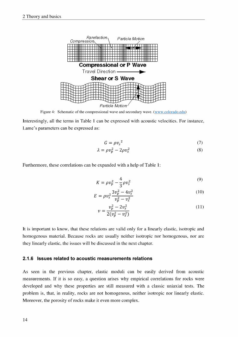
Figure 4: Schematic of the compressional wave and secondary wave.
(www.colorado.edu) ................................................................................... 14
Figure 5: Static and dynamic bulk moduli as measured during a hydrostatic test (left)
and static and dynamic moduli as measured during a triaxial test (right).
(Fjaer et al., 2008) ....................................................................................... 15
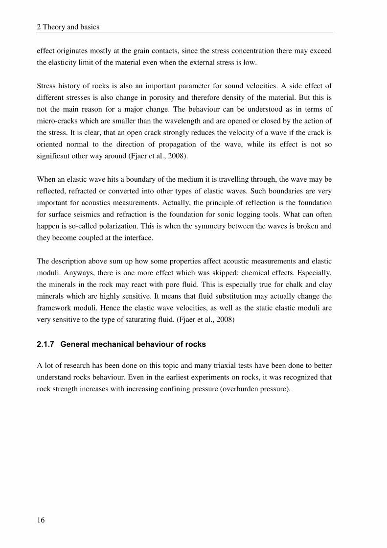
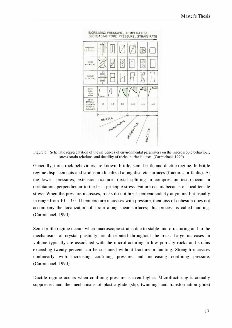
Figure 6: Schenatic representation of the influences of environmental paramaters on
the macroscopic behaviour, stress-strain relations, and ductility of rocks in
triaxial tests. (Carmichael, 1990) ................................................................ 17
Figure 7: Castagna et al. (1993) and Pickett's (1963) correlations for
limestones.(Mavko et al., 1998) ................................................................. 24
Figure 8: Castagna et al. (1993) and Pickett's (1963) correlations for
dolomites.(Mavko et al., 1998) ................................................................... 25
Figure 9: Castagna et al. (1993) and Han's (1986) correlations for sandstones.
(Mavko et al., 1998) .................................................................................... 26
Figure 10: Random results with a line which fits the best. (Modified after Mihailović, 2002) ........................................................................................................... 27
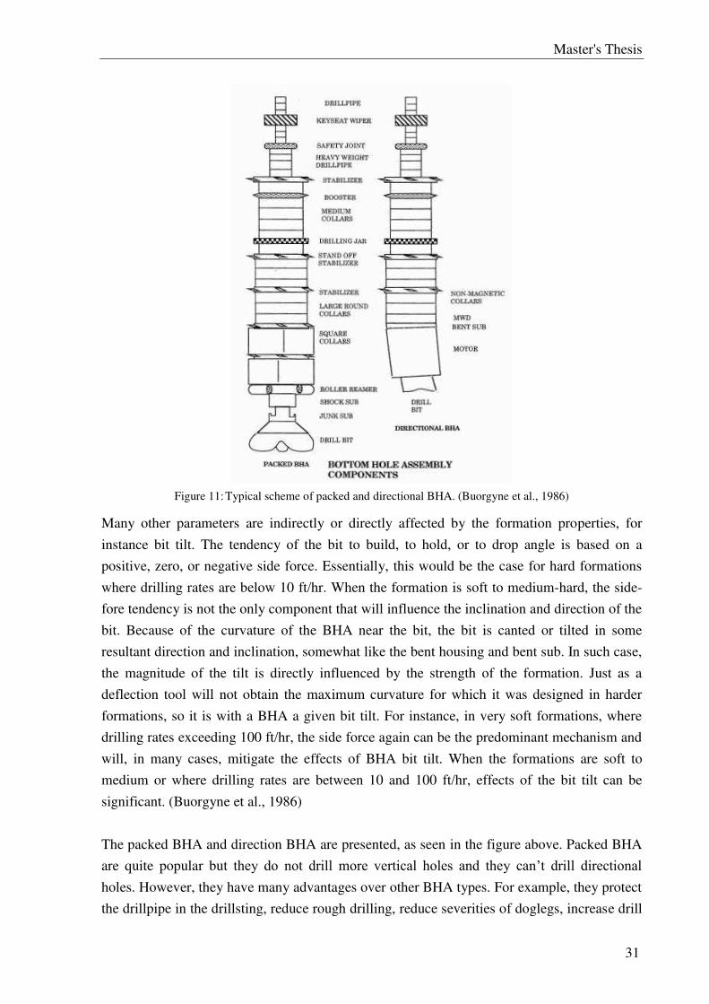
Figure 11: Typical scheme of packed and directional BHA. (Buorgyne et al., 1986) . 31
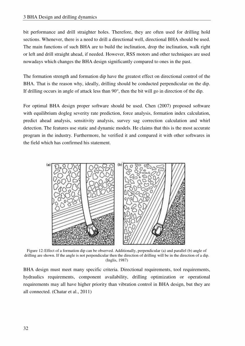
Figure 12: Effect of a formation dip can be observed. Additionally, perpendicular (a)
and parallel (b) angle of drilling are shown. If the angle is not perpendicular
then the direction of drilling will be in the direction of a dip. (Inglis, 1987)
.................................................................................................................... 32
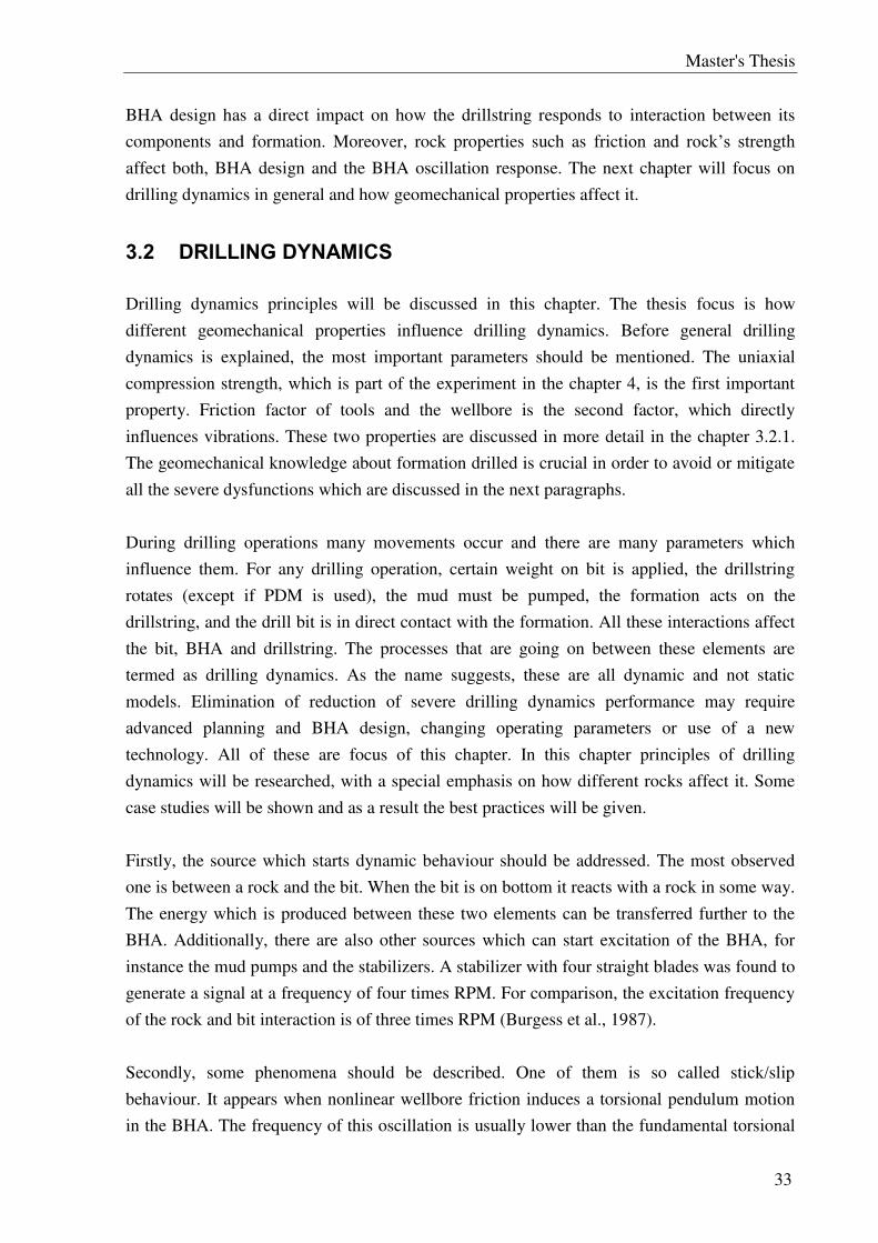
Figure 13: Some of the vibrations in the BHA and their possible consequences.
(Ramizer et al., 2010) ................................................................................. 35
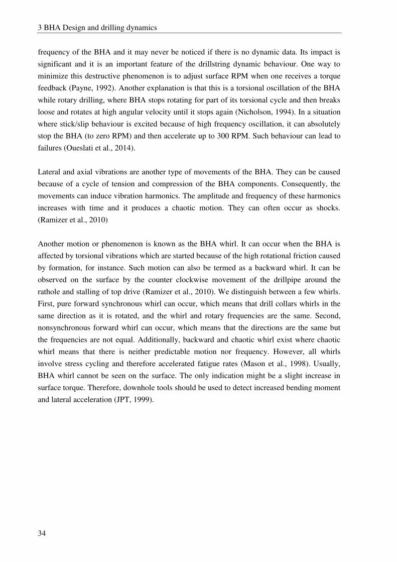
Figure 14: Relationships of some known excitation frequencies to the frequencies of
dynamic behaviour.(Reckmann et al., 2010) .............................................. 35
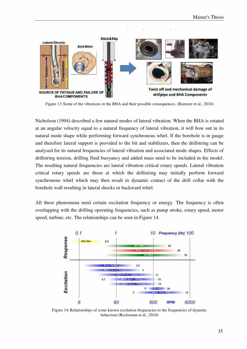
Figure 15: WOB versus rotary speed relation and drilling dynamics dysfunctions
which can occur. (Jain et al. 2014) ............................................................. 36
Figure 16: The figure is representing drilling through loose, soft sandstone with hard
calcite stringers. The question arises what is happening with the BHA in
such conditions. (Modified after Hood et al, 2003) .................................... 38
V
Figure 17: Modular vibration sensor, positioned just after the bit. (left) and a typical
MWD tool (right). (Oueslati et al., 2014) ............................................................. 40
Figure 18: Redesigned BHA which improved drilling time for 300%. ................................. 41
Figure 19: Failure rate (probability) versus lateral 1s RMS accelaration threshold and
time. (Reckmann et al., 2010) ............................................................................... 44
Figure 20: RPM vs. WOB stability diagram for drilling 24 inch well through the
sandstone developed by Elsborg et al. (2006). ..................................................... 46
Figure 21: RPM adjustment while drilling 24 inch hole. ....................................................... 46
Figure 22: The overcored limestone sample which was used in the experiment. .................. 50
Figure 23: Carbonate reservoirs around the world. (Ehrenberg et al., 2005) ......................... 51
Figure 24: The broken part of the limestone sample. Foliation where the sample broke
is clearly visible. ................................................................................................... 51
Figure 25: The overcored sandstone sample which was used in the experiment. .................. 52
Figure 26: Sandstone reservoirs around the world. (Ehrenberg et al., 2005) ......................... 53
Figure 27: A schematic view of the ultrasonic device. (Gegenhuber, 2015) ......................... 55
Figure 28: The experimental setup; Generator Geotron USG 40, receiver, transducer
and a sample. ........................................................................................................ 55
Figure 29: Limestone (left) and sandstone (right) sample in the measurement cell. ............. 56
Figure 30: The rocks from which the samples were cored. ................................................... 57
Figure 31: A typical setup for uniaxial compression test. (Mwanga et al., 2015) ................. 57
Figure 32: Both samples loaded into the cell; limestone (left) and sandstone (right). ........... 59
Figure 33: Duration of the UCS test, when limestone sample was loaded. ........................... 61
Figure 34: Force - strain curve for the limestone sample. ...................................................... 61
Figure 35: The limestone breakage. ....................................................................................... 62
Figure 36: Duration of the UCS test, when sandstone sample was loaded. ........................... 62
Figure 37: Force - strain curve fort the sandstone sample. .................................................... 63
Figure 38: The sandstone breakage. ....................................................................................... 64
Figure 39: A flow chart showing the procedure of obtaining rock properties in a new
field with numerous coring samples available. ..................................................... 67
Figure 40: A flow chart showing the procedure of obtaining rock properties in a new
field with limited coring samples available. ......................................................... 68

VI
List of Symbols and Abbreviations
NPT Non-productive Time
MWD Measured While Drilling
LWD Logging While Drilling
BHA Bottomhole Assembly
GOR Gas Oil Ratio
M Molecular weight Velocity at temperature T Initial velocity Pressure in the x-direction [Pa] Strain in the x-direction [1] Young’s modulus [Pa] Poisson’s ratio [1] λ Lame’s first parameter G Modulus of rigidity [Pa]
K Bulk modulus [Pa] Primary wave velocity [m/s] Secondary wave velocity [m/s]
UCS Uniaxial Compressive Strength Travel time [s] or [µs/ft] Density [kg/m3] Clay fraction [1] Porosity [1]
RSS Rotary Steerable System
HFTO High Frequency Torsional Oscillation
LFTO Low Frequency Torsional Oscillation
FSS Full Stick Slip
VII
Table of contents
1 Introduction .................................................................................................... 1
2 Theory and basics ........................................................................................... 5
2.1 Rock Properties ............................................................................................................ 5
2.1.1 Introduction .......................................................................................................... 5
2.1.2 Density and porosity ............................................................................................. 6
2.1.3 Fluid properties – acoustic .................................................................................... 9
2.1.4 Elastic moduli ..................................................................................................... 11
2.1.5 P- and S- waves .................................................................................................. 13
2.1.6 Issues related to acoustic measurements relations .............................................. 14
2.1.7 General mechanical behaviour of rocks ............................................................. 16
2.2 Log derivative methods ............................................................................................. 18
2.2.1 Determination of sandstone rock properties ....................................................... 18
2.2.1.1 Strength as a function of porosity for sandstone ........................................ 18
2.2.1.2 Strength as a function of sonic velocity or travel time ................................ 20
2.2.1.3 Strength as a function of Young’s modulus ................................................ 21
2.2.2 Correlations for carbonates ................................................................................. 22
2.2.2.1 Strength as a function of porosity ............................................................... 22
2.2.2.2 Rock Strength as a function of Sonic Velocity/Travel Time ...................... 22
2.2.3 Correlations for shales ........................................................................................ 23
2.3 VP – VS Relations ....................................................................................................... 23
2.4 Velocity – density relations ....................................................................................... 26
2.5 Linear Correlations .................................................................................................... 27
3 BHA Design and drilling dynamics ............................................................. 30
3.1 BHA Design ............................................................................................................... 30
3.2 Drilling dynamics ...................................................................................................... 33
3.2.1 Formation effects on drilling dynamics .............................................................. 36
3.2.2 Issues with the measurements of drilling dynamics ........................................... 39
3.2.3 Case study 1 – Ramizer et al., 2010 ................................................................... 41
3.2.4 Case study 2 – Mason et al. (1998) .................................................................... 42
VIII
3.2.5 Case study 3 – Bailey et al. (2009) .................................................................... 42
3.2.6 Case study 4 – Reckmann et al. (2010) .............................................................. 43
3.2.7 Case study 5 – Elsborg et al. (2006) .................................................................. 44
3.2.8 The case studies summary and lessons learned ................................................. 47
4 Experimental setup ....................................................................................... 49
4.1 Description of the Samples........................................................................................ 49
4.2 Measurements description ......................................................................................... 54
4.2.1 Ultrasound and porosity measurements ............................................................. 54
4.2.2 The UCS test procedure ..................................................................................... 57
5 Results and discussion .................................................................................. 60
5.1 Experimental results .................................................................................................. 60
5.1.1 Ultrasound measurements .................................................................................. 60
5.1.2 The UCS tests..................................................................................................... 60
5.1.3 Comparison of the correlations with the UCS test values ................................. 64
5.1.4 Process of obtaining rock properties from logs ................................................. 65
5.1.5 Advantages and Disadvantages of Obtaining Rock Properties from Logs ........ 69
5.2 Recommended practices to avoid drilling dynamics dysfunctions ........................... 69
5.2.1 Full Stick Slip (FSS) .......................................................................................... 70
5.2.2 Low Frequency Torsional Oscillation (LFTO) .................................................. 70
5.2.3 High Frequency Torsional Oscillation (HFTO) ................................................. 70
5.2.4 Random Torsional Vibration ............................................................................. 70
5.2.5 BHA Whirl ......................................................................................................... 71
6 Conclusion .................................................................................................... 72
7 References .................................................................................................... 74
Master's Thesis
1
1 INTRODUCTION
Wells in the oil and gas industry are becoming increasingly complex and are drilled through
formations which were previously unreachable. Due to the nature of such complexity, the risk
of various hazards increases and, therefore, more data is needed. One of the challenges is
associated with geomechanical evaluation. Issues like wellbore stability, bit selection, BHA
design, drilling dynamics and stuck pipe can be affected by a lack of geomechanical data.
Specifically, the information is critical for the successful drilling of directional, highly
deviated or horizontal wells. During drilling, the data provides the information required to
conduct safe operations and to minimise both NPT and trouble time, whilst maximising
drilling efficiency.
A lot of time and money are lost due to NPT associated with drilling troubles, which happen
due to poor wellbore stability. It is well known that rock properties information increases the
effectiveness of drilling and NPT can be significantly reduced if good practices are
considered. Due to a lack of geomechanical information, many wells around the world do not
reach their planned target depth and have difficulties while drilling, such as stuck pipe, tool
failures and wellbore instability (York et al, 2009).
Sonic, resistivity, density or gamma ray logs can be used to estimate in situ mechanical rock
properties. These techniques are in use as an alternative to costly and time consuming
laboratory tests. The rock properties which are usually determined include UCS, friction
angle, cohesion and rock elastic constants, for example, Young’s modulus, Poisson’s ratio, bulk modulus and shear modulus. This technique has a number of advantages over laboratory
measurements (and coring operation) of geomechanical properties, including availability,
providing continuous profiles, its low cost and time effectiveness (Odunlami et al., 2011).
Relationships between rocks’ physical and mechanical properties were established more than 70 years ago. Wyllie et al. (1956) introduced an empirical relationship between porosity and
acoustic velocity of a porous media. The porosity correlation is still widely used today as it
gives good results. Many correlations were found in subsequent years, after the introduction.
Successful derivation of rock strength based on porosity was conducted on sandstones,
carbonates and shales (Sarda et al., 1993, Edlmann et al., 1998, Farquahar et al., 1994, Raaen
et al., 1996 and Chang et al., 2006). Rock strength parameters were also determined with the
help of Young’s modulus (Perkins et al., 1995, Bradford et al., 1998). It was demonstrated that, as porosity increases, elastic moduli, along with UCS, cohesion and angle of internal
friction, all decrease (Edlmann et al., 1998, Farquhar et al., 1994).
1 Introduction
2
It is often the case that a sonic log or other logs are unavailable. For example, Santana et al.
(2010) developed a correlation between resistivity and sonic log data. The methodology to
match these two measurements as accurately as possible was developed and applied on case
studies from wells drilled in the Gulf of Mexico.
A new method for estimating in situ mechanical properties from logs was presented in 1996
(Raaen et al.). This method compared the results from more than 200 rock mechanical tests
made on cores. The main advantage of this model is that it can be applied to new wells and
fields without re-calibration. The authors suggest that a minor calibration can be applied, even
though it is not needed. The sensitivity analysis proved that the method is satisfactorily
robust.
Odunlami et al. (2011) presented an innovative management platform, where rock parameters
were determined exclusively by use of log data. They used all the major empirical methods
and concluded that empirical correlations are capable of being used in situations where core
data is not readily available. However, local calibration should be completed for a different
location. The best correlation gave porosity measurement, as it returned the best estimate of
UCS when compared with lab derived core UCS.
Borba et al. (2014) discovered a connection between standard uniaxial test, scratch test and
log-based empirical correlation, which were found to be in a good agreement. They suggest
that the results can be extrapolated to the entire interval of interest and, furthermore, that the
values determined indirectly should be calibrated.
Chang et al. (2006) completed a brief study of different correlation models. The models were
evaluated and a large set of data was used to calculate and compare results with physical
property data from the literature. It was concluded that some equations work reasonably well,
whereas individual rock strength variations with individual physical properties scatter
considerably. Therefore, local calibration is suggested.
When the rock properties are defined, an evaluation of other operational phenomena can
begin, such as drilling dynamics, which is the logical continuation once the rock properties
are obtained with the help of the empirical correlations described above. Drilling dynamics is
defined as being all of the dynamic movements of the drill string, which occur at certain
frequencies due to an applied load, or interaction between two elements (for example, the drill
string and the wall). In this thesis, special focus will be given on the BHA drilling dynamics,
how the dynamics are affected by rock properties (especially UCS) and the resultant effect on
drilling operations.
Master's Thesis
3
A great deal of research has been carried out on drilling dynamics, the severe behaviour of
which forced oil companies to seek to prevent the problem, with many failures being reported
in the literature. MWD tools, roller reamers, joints, LWD and other tools failed due to drilling
dynamics dysfunctions (Payne, 1992, Chen, 2007, Mason, 1998, Chatar et al., 2011, Ramizer
et al., 2010, Bailey et al., 2009).
In addition, to change operating parameters and introduce real time monitoring, a proper
planning and BHA design should be prepared to prevent drilling dynamics dysfunctions. The
most common phenomena are BHA whirl and stick-slip, which can occur as a result of
torsional movements, bit bounce and torsional accelerations. All these effects can contribute
to significant NPT which, consequently, increases both the drilling time and costs of the well.
After taking proper steps to mitigate or eliminate these dysfunctions, NPT decreased up to
40% in some cases (Bailey et al., 2009, Burgess et al., 1987, Reckmann et al., 2010).
It was difficult to evaluate the drilling dynamics until the proper measurement devices
appeared. It had previously been thought that high frequency vibrations did not damage either
the tools or the wellbore. It was later discovered, with the help of high frequency
measurements, that they can cause significant and severe excitations which may lead to tools
failure (Oueslati et al., 2013). Therefore, at present, all the frequencies are measured, in order
to get a full picture of drilling dynamics.
The thesis objectives
Several objectives are set for the thesis. Most of the correlations found in the literature are
stated in the thesis. Additionally, limestone correlations from Farquhar et al. (1994), Militzer
(1973), Golubev (1973) and Chang et al. (2006) and sandstone correlations from Freyburg
(1972), Vernik et al. (1993), Farquhar et al. (1994), Sarda et al. (1993), Raeen et al. (1996),
Moor et al. (1999), Rahman et al. (2010), and Chang et al. (2006) are used in order to meet
the following objectives:
1. Comparison of the correlations above with an experiment in which a sandstone and
limestone samples are tested. Sonic velocity, porosity and UCS values are measured
on both samples. As a result, the sonic velocity and porosity values are used in the
correlations and compared to the UCS values obtained in a laboratory.
2. Usage of the empirical correlations is verified, including their impact on cost –
effectivness, time savings and information quality.
3. Derivation of recommended procedures how to use the empirical correlations in a new
field.
Drilling dynamics is an important phenomenon, which occurs during drilling operations and
its knowledge can help with drilling the well on time, reduce NPT and hit the target. Drilling

1 Introduction
4
dynamics is dependent on rock properties. Therefore, the relationship between them is
studied in the thesis with the following objectives set:
1. How a formation dip affects drilling dynamics.
2. Influence of friction factor on BHA vibrations.
3. Drilling dynamics response to hard rocks (high UCS) stringers within a soft and loose
formation.
Master's Thesis
5
2 THEORY AND BASICS
2.1 ROCK PROPERTIES
2.1.1 Introduction
Because the thesis is dealing with rock properties and their effect on BHA design and drilling
dynamics, this chapter will provide some theory about them. General rock properties will be
described and the most common rocks which appear in the oil and gas industry discussed.
Rocks are defined as aggregates of minerals plus pore space which can be empty or filled with
a fluid. In general, the three major rock types are classified as igneous, metamorphic and
sedimentary. (Lake, 2007)
Minerals have definite structure, composition and properties which are dependent on their
chemistry and structure. There are hundreds of minerals in the Earth’s crust but in the oil and gas industry we usually deal with rather low number of them. They can be broken into
silicates, sulphates, sulphides, carbonates, and oxides. Often, organic compounds such as coal
or bitumen are present. Classification can be further broken into the most common used
elements in the oil and gas industry (Lake, 2007):
Common silicates:
- Quartz.
- Feldspars.
- Micas.
- Zeolites.
- Clays.
Common carbonates:
- Calcite
- Dolomite
- Siderite may be present.
Oxides:
- Magnetite
- Hematite
Usually, the knowledge about quartz, feldspars, clays, calcite, dolomite and anhydrite is
enough to fulfil most engineering needs.
2 Theory and basics
6
One of the most problematic minerals and the least understood are clays. They are
problematic because their properties change significantly with in-situ pressure, temperature
and chemical environment. Parts of clays can be presented in other rocks, for instance in
sandstone, which makes the understanding about rocks behaviour significantly more difficult.
(Lake, 2007)
2.1.2 Density and porosity
Density and porosity are one of the most important parameters, which further affect properties
such as the strength, acoustic velocities, elasticity and others. Density of rocks is more
complex because of many phases presented inside the void spaces.
The basic definition of density is mass per volume. For homogeneous or single-phase
material, the definition of density is simple. However, rocks are usually mixtures of several
phases, both solids and fluids.
Porosity directly affects density because a fluid is always present in pores. It is defined as the
nonsolid or pore-volume fraction. It is worth mentioning different volumes, which are often
used. For instance, total volume of rock, volume of mineral phase, volume of pores or
openings, volume of interconnected pores, volume of isolated pores, volume of cracks or
fractures and volume of different fluid phases. From these we can define the various kinds of
porosity such as total porosity, effective porosity, ineffective porosity and crack or fracture
porosity.
The figure below shows how porosity is dependent on density and vice-versa.
Master's Thesis
7
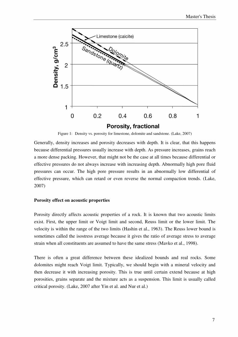
Figure 1: Density vs. porosity for limestone, dolomite and sandstone. (Lake, 2007)
Generally, density increases and porosity decreases with depth. It is clear, that this happens
because differential pressures usually increase with depth. As pressure increases, grains reach
a more dense packing. However, that might not be the case at all times because differential or
effective pressures do not always increase with increasing depth. Abnormally high pore fluid
pressures can occur. The high pore pressure results in an abnormally low differential of
effective pressure, which can retard or even reverse the normal compaction trends. (Lake,
2007)
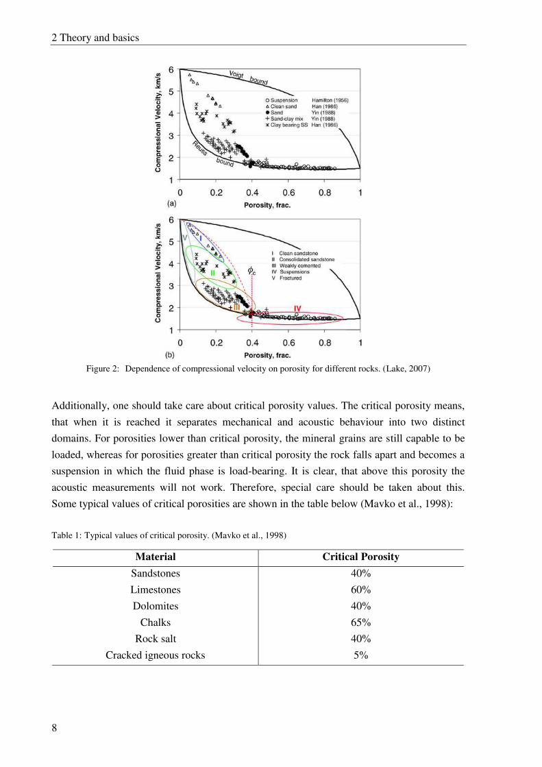
Porosity effect on acoustic properties
Porosity directly affects acoustic properties of a rock. It is known that two acoustic limits
exist. First, the upper limit or Voigt limit and second, Reuss limit or the lower limit. The
velocity is within the range of the two limits (Hashin et al., 1963). The Reuss lower bound is
sometimes called the isostress average because it gives the ratio of average stress to average
strain when all constituents are assumed to have the same stress (Mavko et al., 1998).
There is often a great difference between these idealized bounds and real rocks. Some
dolomites might reach Voigt limit. Typically, we should begin with a mineral velocity and
then decrease it with increasing porosity. This is true until certain extend because at high
porosities, grains separate and the mixture acts as a suspension. This limit is usually called
critical porosity. (Lake, 2007 after Yin et al. and Nur et al.)
2 Theory and basics
8
Figure 2: Dependence of compressional velocity on porosity for different rocks. (Lake, 2007)
Additionally, one should take care about critical porosity values. The critical porosity means,
that when it is reached it separates mechanical and acoustic behaviour into two distinct
domains. For porosities lower than critical porosity, the mineral grains are still capable to be
loaded, whereas for porosities greater than critical porosity the rock falls apart and becomes a
suspension in which the fluid phase is load-bearing. It is clear, that above this porosity the
acoustic measurements will not work. Therefore, special care should be taken about this.
Some typical values of critical porosities are shown in the table below (Mavko et al., 1998):
Table 1: Typical values of critical porosity. (Mavko et al., 1998)
Material Critical Porosity
Sandstones 40%
Limestones 60%
Dolomites 40%
Chalks 65%
Rock salt 40%
Cracked igneous rocks 5%
Master's Thesis
9
2.1.3 Fluid properties – acoustic
Rocks consist of pores and they can contain different fluids. The fluid inside the pores could
be water, air, oil or gas. The properties of fluids are needed if we wish to interpret the
laboratory data or in-situ data from logs or seismic measurements. Logging tools are greatly
affected by acoustic properties of a fluid, which is in the pores. The fluid acoustic properties
are dependent on temperature, pressure, overburden stress and others. The same fluid could
behave differently under different circumstances.
Oil
The oil itself has already different properties – it can be a heavy or very light oil. Because of
its properties the oil can transform from liquid phase to a quasi-solid phase with drastic
increase of viscosity. Therefore, P-wave velocity and S-wave velocity change drastically. In
some cases the velocity can change up to 50%. It is clear that a fluids composition should be
evaluated carefully. Additionally, the velocities are highly dependent on GOR (Gas-Oil
Ratio), temperature and pressure of the oil. (Han et al., 2006)
It is a well-known fact that sound velocity depends on media. In the air, the speed of sound is
1.236 km/h. In water the speed increases for more than four times, up to 5.342 km/h and in
solids like rocks or metals the speed is the highest. Please note that the speeds stated before
are in ideal conditions. Like stated before the velocity can change significantly when
temperature or pressure changes. A problem which may arise when dealing with different
fluids is that the composition of the fluid is rarely known.
Many correlations describe how moduli typically increases with increasing temperature and
increases with increasing pressure. Wang and Nur (1998) did an extensive study of several
hydrocarbons and found simple relationships among the density, moduli, temperature and
carbon number (Lake, 2007):
(1)
where is the initial velocity, is the velocity at temperature T, is the temperature
change, and b is a constant for each compound of molecular weight M:
(2)
Similarly, the velocities are related in molecular weight by:
2 Theory and basics
10
(3)
where is the velocity of oil of weight M, and is the velocity of a reference oil of
weight at temperature T0. The variable is a positive function of temperature. It is
clearly visible that the velocity of the fluid will increase with increasing molecular weight.
However, more complex compositions can occur and the influence of pressure should be
considered as well.
For predicting the frequency-dependent velocities of saturated rocks in terms of the dry rock
properties, formulas were derived by Biot (1956). The formulas incorporate some of the
mechanisms of viscous and inertial interaction between the pore fluid and the mineral matrix
of the rock. The formulas are based on the limiting velocities which are the same as predicted
by Gassmann’s relations (Mavko et al., 1998).
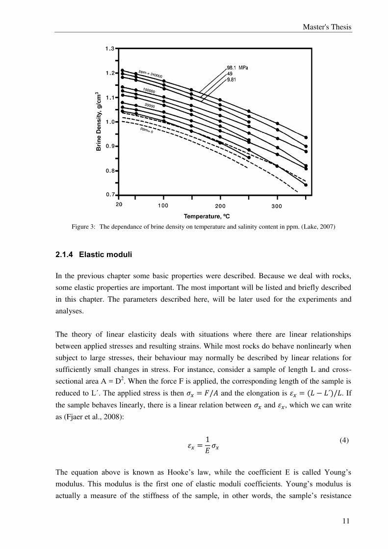
Brines
The most common fluid during drilling through different rock masses consist of brines. Their
composition can range from pure water to saturated saline solutions. The concentration of
brines can vary from field to field. Salinity of brines is an important parameter because it
obviously increases their density. Many correlations to calculate density of a brine were
developed. Due to different density of brines the sound velocity can greatly differ from brine
to brine. (Lake, 2007)
Master's Thesis
11
Figure 3: The dependance of brine density on temperature and salinity content in ppm. (Lake, 2007)
2.1.4 Elastic moduli
In the previous chapter some basic properties were described. Because we deal with rocks,
some elastic properties are important. The most important will be listed and briefly described
in this chapter. The parameters described here, will be later used for the experiments and
analyses.
The theory of linear elasticity deals with situations where there are linear relationships
between applied stresses and resulting strains. While most rocks do behave nonlinearly when
subject to large stresses, their behaviour may normally be described by linear relations for
sufficiently small changes in stress. For instance, consider a sample of length L and cross-
sectional area A = D2. When the force F is applied, the corresponding length of the sample is
reduced to L´. The applied stress is then and the elongation is . If
the sample behaves linearly, there is a linear relation between and , which we can write
as (Fjaer et al., 2008):
(4)
The equation above is known as Hooke’s law, while the coefficient E is called Young’s modulus. This modulus is the first one of elastic moduli coefficients. Young’s modulus is actually a measure of the stiffness of the sample, in other words, the sample’s resistance
2 Theory and basics
12
against being compressed by the uniaxial stress (Fjaer et al., 2008). A perfectly rigid material
has an infinite Young’s modulus, because an infinite force is needed to deform such a material. Therefore, it can be said that material which has a high Young’s modulus is approximated as rigid.
If a stress is applied, there will be another consequence; an increase in width D of the sample.
The lateral elongation is defined as . The ratio between axial and
lateral elongations is defined as:
(5)
This is another important elastic parameter, known as Poisson’s ratio. It is a measure of lateral expansion relative to longitudinal contraction. Most materials have Poisson’s ratio between 0.0 and 0.5. If the material is ideally incompressible at small strains, then the material would
have Poisson’s ratio of exactly 0.5. On the contrary, a material which shows little lateral expansion when compressed would have Poisson’s ratio of 0, such as unconsolidated sands.
There are some materials which can reach the negative ratio, for instance, weak porous rocks.
Typically, for rocks Poisson’s ratio is between 0.15 – 0.25.
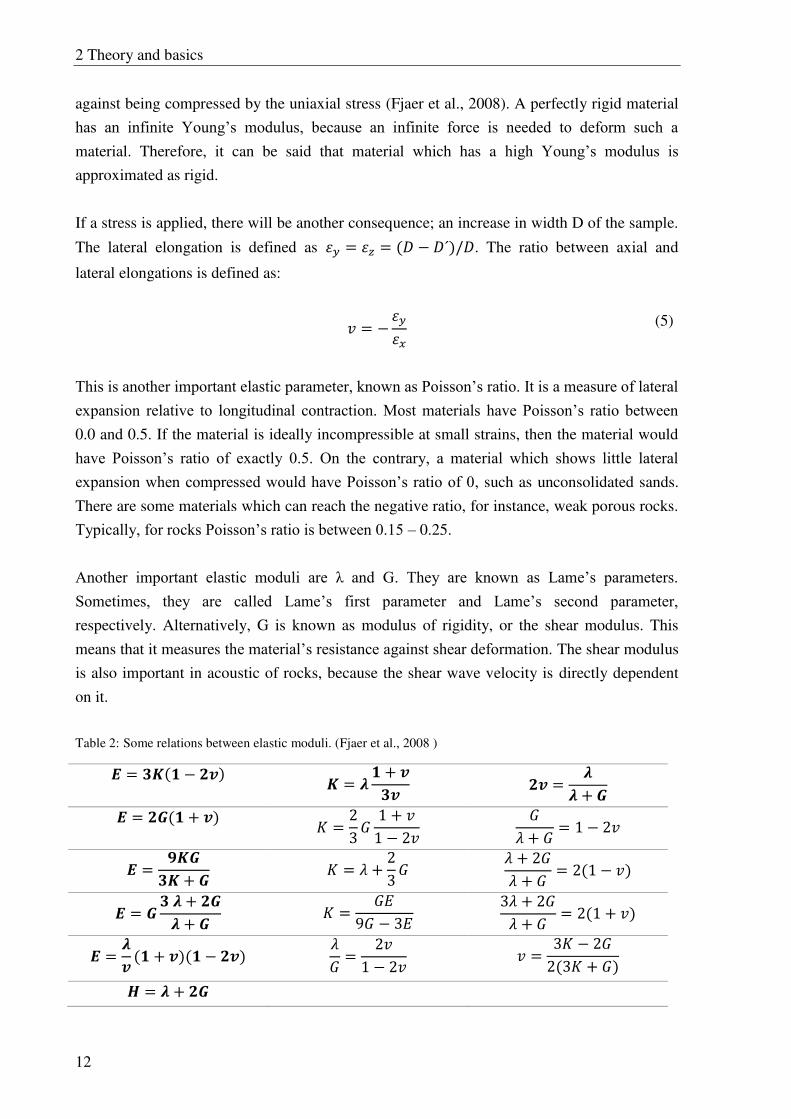
Another important elastic moduli are λ and G. They are known as Lame’s parameters. Sometimes, they are called Lame’s first parameter and Lame’s second parameter, respectively. Alternatively, G is known as modulus of rigidity, or the shear modulus. This
means that it measures the material’s resistance against shear deformation. The shear modulus
is also important in acoustic of rocks, because the shear wave velocity is directly dependent
on it.
Table 2: Some relations between elastic moduli. (Fjaer et al., 2008 )
Master's Thesis
13
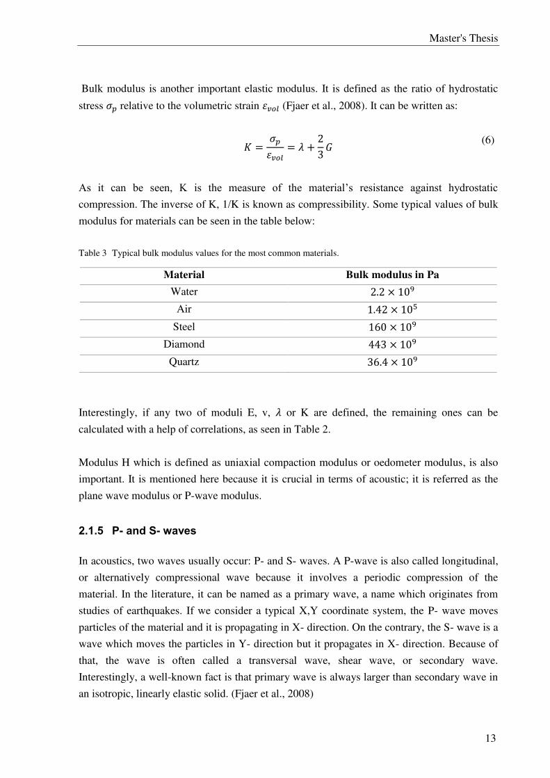
Bulk modulus is another important elastic modulus. It is defined as the ratio of hydrostatic
stress relative to the volumetric strain (Fjaer et al., 2008). It can be written as:
(6)
As it can be seen, K is the measure of the material’s resistance against hydrostatic compression. The inverse of K, 1/K is known as compressibility. Some typical values of bulk
modulus for materials can be seen in the table below:
Table 3 Typical bulk modulus values for the most common materials.
Material Bulk modulus in Pa
Water
Air
Steel
Diamond
Quartz
Interestingly, if any two of moduli E, v, or K are defined, the remaining ones can be
calculated with a help of correlations, as seen in Table 2.
Modulus H which is defined as uniaxial compaction modulus or oedometer modulus, is also
important. It is mentioned here because it is crucial in terms of acoustic; it is referred as the
plane wave modulus or P-wave modulus.
2.1.5 P- and S- waves
In acoustics, two waves usually occur: P- and S- waves. A P-wave is also called longitudinal,
or alternatively compressional wave because it involves a periodic compression of the
material. In the literature, it can be named as a primary wave, a name which originates from
studies of earthquakes. If we consider a typical X,Y coordinate system, the P- wave moves
particles of the material and it is propagating in X- direction. On the contrary, the S- wave is a
wave which moves the particles in Y- direction but it propagates in X- direction. Because of
that, the wave is often called a transversal wave, shear wave, or secondary wave.
Interestingly, a well-known fact is that primary wave is always larger than secondary wave in
an isotropic, linearly elastic solid. (Fjaer et al., 2008)
Master's Thesis
15
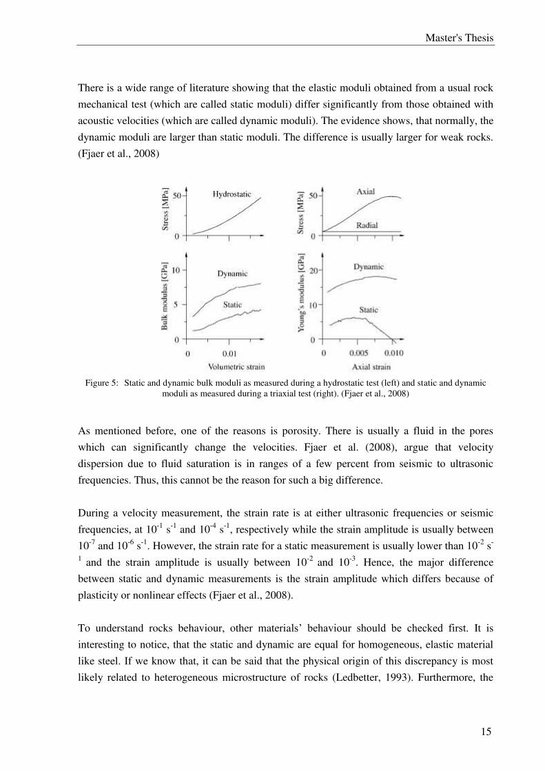
There is a wide range of literature showing that the elastic moduli obtained from a usual rock
mechanical test (which are called static moduli) differ significantly from those obtained with
acoustic velocities (which are called dynamic moduli). The evidence shows, that normally, the
dynamic moduli are larger than static moduli. The difference is usually larger for weak rocks.
(Fjaer et al., 2008)
Figure 5: Static and dynamic bulk moduli as measured during a hydrostatic test (left) and static and dynamic
moduli as measured during a triaxial test (right). (Fjaer et al., 2008)
As mentioned before, one of the reasons is porosity. There is usually a fluid in the pores
which can significantly change the velocities. Fjaer et al. (2008), argue that velocity
dispersion due to fluid saturation is in ranges of a few percent from seismic to ultrasonic
frequencies. Thus, this cannot be the reason for such a big difference.
During a velocity measurement, the strain rate is at either ultrasonic frequencies or seismic
frequencies, at 10-1
s-1
and 10-4
s-1
, respectively while the strain amplitude is usually between
10-7
and 10-6
s-1
. However, the strain rate for a static measurement is usually lower than 10-2
s-
1 and the strain amplitude is usually between 10
-2 and 10
-3. Hence, the major difference
between static and dynamic measurements is the strain amplitude which differs because of
plasticity or nonlinear effects (Fjaer et al., 2008).
To understand rocks behaviour, other materials’ behaviour should be checked first. It is
interesting to notice, that the static and dynamic are equal for homogeneous, elastic material
like steel. If we know that, it can be said that the physical origin of this discrepancy is most
likely related to heterogeneous microstructure of rocks (Ledbetter, 1993). Furthermore, the
2 Theory and basics
16
effect originates mostly at the grain contacts, since the stress concentration there may exceed
the elasticity limit of the material even when the external stress is low.
Stress history of rocks is also an important parameter for sound velocities. A side effect of
different stresses is also change in porosity and therefore density of the material. But this is
not the main reason for a major change. The behaviour can be understood as in terms of
micro-cracks which are smaller than the wavelength and are opened or closed by the action of
the stress. It is clear, that an open crack strongly reduces the velocity of a wave if the crack is
oriented normal to the direction of propagation of the wave, while its effect is not so
significant other way around (Fjaer et al., 2008).
When an elastic wave hits a boundary of the medium it is travelling through, the wave may be
reflected, refracted or converted into other types of elastic waves. Such boundaries are very
important for acoustics measurements. Actually, the principle of reflection is the foundation
for surface seismics and refraction is the foundation for sonic logging tools. What can often
happen is so-called polarization. This is when the symmetry between the waves is broken and
they become coupled at the interface.
The description above sum up how some properties affect acoustic measurements and elastic
moduli. Anyways, there is one more effect which was skipped: chemical effects. Especially,
the minerals in the rock may react with pore fluid. This is especially true for chalk and clay
minerals which are highly sensitive. It means that fluid substitution may actually change the
framework moduli. Hence the elastic wave velocities, as well as the static elastic moduli are
very sensitive to the type of saturating fluid. (Fjaer et al., 2008)
2.1.7 General mechanical behaviour of rocks
A lot of research has been done on this topic and many triaxial tests have been done to better
understand rocks behaviour. Even in the earliest experiments on rocks, it was recognized that
rock strength increases with increasing confining pressure (overburden pressure).
Master's Thesis
17
Figure 6: Schenatic representation of the influences of environmental paramaters on the macroscopic behaviour,
stress-strain relations, and ductility of rocks in triaxial tests. (Carmichael, 1990)
Generally, three rock behaviours are known: brittle, semi-brittle and ductile regime. In brittle
regime displacements and strains are localized along discrete surfaces (fractures or faults). At
the lowest pressures, extension fractures (axial splitting in compression tests) occur in
orientations perpendicular to the least principle stress. Failure occurs because of local tensile
stress. When the pressure increases, rocks do not break perpendicularly anymore, but usually
in range from 10 – 35°. If temperature increases with pressure, then loss of cohesion does not
accompany the localization of strain along shear surfaces; this process is called faulting.
(Carmichael, 1990)
Semi-brittle regime occurs when macroscopic strains due to stable microfracturing and to the
mechanisms of crystal plasticity are distributed throughout the rock. Large increases in
volume typically are associated with the microfracturing in low porosity rocks and strains
exceeding twenty percent can be sustained without fracture or faulting. Strength increases
nonlinearly with increasing confining pressure and increasing confining pressure.
(Carmichael, 1990)
Ductile regime occurs when confining pressure is even higher. Microfracturing is actually
suppressed and the mechanisms of plastic glide (slip, twinning, and transformation glide)
2 Theory and basics
18
dominate at low to intermediate temperatures. The slope of the stress-strain curve is
insensitive to changes in confining pressure. (Carmichael, 1990)
2.2 LOG DERIVATIVE METHODS
All the available correlations which can be found in literature will be given and listed in this
chapter. They are developed mainly for sandstones, carbonates (limestone, dolomite) and
shales. Therefore, they are split into three categories. Furthermore, they are derived from
either porosity, travel time and sonic speed or Young’s modulus. These correlations will be
later on applied on the real samples in the chapter “experiments”.
2.2.1 Determination of sandstone rock properties
2.2.1.1 Strength as a function of porosity for sandstone
According to Vernik et al (1993) porosity was identified as the best predictor of rock strength
in sedimentary rocks. The research included 52 cores of carbonate poor siliciclastic rocks
from a broad range of sedimentary basins on which 195 drained, compressive triaxial tests
were conducted including 27 unconfined tests. The porosities varied between 1% and 36%.
They classified the core samples into arenites and clean arenites (volume of clay less 3% and
3-15%, respectively) and derived the following empirical correlation (Odunlami et al., 2011):
(12)
where UCS is in MPa and is in percentage. The equation has been claimed to have a global
application for sandstones.
Edlmann et al. (1998) claimed that porosity gives a better continuous representation and a
wider scope rock properties than acoustic data. Therefore, they were focused on finding
relationships between log-derived porosity and rock mechanical properties. Additionally, they
stated empirical correlations between porosity and other rock properties such as elastic
moduli, strength moduli, cohesion, angle of internal friction, Poisson’s ratio and stress factor.
For uniaxial compressive strength (UCS) the following correlation was found:
(13)
where UCS is in MPa and is in percentage. Authors claim that the correlation can be
applied on a wide range of sandstones.
Master's Thesis
19
Farquhar et al. (1994) determined another set of correlations for sandstones and carbonates.
UCS, static and dynamic elastic modules were determined. They claim that the correlation
should be used with caution, because they provide an estimate of the mechanical properties
when core material is not available for testing. The correlation of UCS for sandstones is as
follows:
(14)
where UCS is in MPa and is in percentage.
Sarda et al. (1993) evaluated compressive strength based on logs from a well on Germigny-
sous-Coulombs structure. The relationships between compressive strength and porosity were
developed using a theoretical approach of grain contacts, the analysis of published rock
mechanics data and mechanical measurements on plugs taken from well cores. The
relationships were primarily found to prevent sand production. The correlations were found
for a set of porosities:
(15)
(16)
(17)
where UCS is in MPa and is in percentage. The correlations were found on many different
types of sandstone.
Raaen et al. (1996) developed an alternate method for estimating in situ rock properties from
logs. The model is based on processes which occur in rocks during mechanical loading. They
focused on the mechanisms which give rise to differences between static and dynamic elastic
moduli. These mechanisms were included into their model. Afterwards, they compared the
results with data from laboratory tests on 235 core samples from several fields in the North
Sea and mid-Norway. A correlation coefficient of 0.88 was achieved and following
correlation found:
(18)
where UCS is in MPa and is in percentage. The equation should be only used for porosities
in a range from 0.2 to 0.35.
2 Theory and basics
20
Chang et al. (2006) developed a correlation for carbonates. They did not state for which area
the correlation works the best, but it can be assumed that it is applicable worldwide. It works
the best for sandstones with UCS between 2 and 360 MPa, with porosity between 0.002 and
0.33.
(19)
Where UCS is in MPa and is in fraction.
2.2.1.2 Strength as a function of sonic velocity or travel time
In the literature review of Chang et al. (2006) a correlation for sandstones in Thuringia region,
Germany can be found. The correlation was developed by Freyburg (1972):
(20)
Where UCS is in MPa nad Vp is in m/s.
Raaen et al. (1996) developed a method for in situ properties of sandstones. The method is
based on compressional sonic log. They claim that it works the best for estimating strength at
non-zero confining stress and for porosities under 35%. Additionally, the validity range of
travel time is between 90 and 140 µs/ft. The equation is as follows:
(21)
Where UCS is in MPa and is in µs/ft.
In order to prevent open hole interval of a wellbore within the Hemlock Sands of the
McArthur River Field, Cook Inlet, Alaska, Moor et al. (1999) developed a correlation for
UCS estimation. They found out that the relationship for the fine-grained sands was
indistinguishable from that for the medium- and coarse-grained sands, and therefore a single
correlation was used:
(22)
Where UCS is in MPa, is density in g/cc and is in m/s. A caution should be taken when
use the correlation because it was used only for clean sandstones and is therefore not
applicable to other lithologies.
Master's Thesis
21
Rahman et al. (2010) proposed a correlation for sandstones in a reservoir in South East Asia.
The correlation was used to prevent sand production from a gas reservoir. The rock strengths
values were derived from multi-stage triaxial tests and correlated with corresponding sonic
travel time:
(23)
Where UCS is in psi and is in µs/ft.
Likewise, Chang et al. (2006) proposed their own correlation after evaluating more than 260
models for sandstones :
(24)
Where UCS is in MPa, is in kg/m3 and Vp is in m/s.
2.2.1.3 Strength as a function of Young’s modulus
According to the literature review, Young’s modulus provides the best estimate for rock strength when the rocks are clastic with large differences in clay content and porosity. This is
due to the fact that Young’s modulus is a measure of rockc matrix which actually bears the
load, and is correlated with the geometry and average number of gran to grain contacts.
(Odunlami 2011 after Plumb 1994)
Often, the best information about rock parameters is not static Young’s modulus but dynamic
one. If dynamic Young’s modulus is known, then rock strength can be calculated with a help of correlation developed by Plumb (1994):
(25)
where UCS is in psi and is in GPa.
Perkins et al. (1995) took samples from 13 fields in the U.S. Gulf Coast area and developed a
correlation with a help of Young’s modulus:
(26)
2 Theory and basics
22
where UCS is in psi, and are in Gpa and is in fraction.
Chang et al. (2006) also found a correlation between Young’s modulus and UCS:
(27)
where E is Young’s modulus in MPa and UCS is in MPa.
2.2.2 Correlations for carbonates
2.2.2.1 Strength as a function of porosity
Farquhar et al. (1994) developed a relationship between porosity and rock strength for
carbonates. The rock samples were from a wide range of reservoirs in the North Sea. The
following correlation was derived:
(28)
Where UCS is in MPa and is in fraction.
2.2.2.2 Rock Strength as a function of Sonic Velocity/Travel Time
As for others, Chang et al. (2006) developed a correlation between travel time and rock
strength:
(29)
Where UCS is in MPa and is in µs/ft. In the paper of Chang et al. (2006) a few other correlations were presented which were
developed by Golubev (1976) and Militzer (1973). They use sonic velocity time to calculate
rock strength.
(Golubev) (30)
(Militzer) (31)
Where UCS is in MPa and is in µs/ft.
Master's Thesis
23
2.2.3 Correlations for shales
Although, shale sections are rarely cored their properties are still important for drilling
operations. They greatly influence wellbore stability, rate of penetration, drilling dynamics
and BHA design.
Horsurd (2001) analysed many cores from the North Sea and the Norwegian Continental
Shelf in order to determine rock strength in shale as a function of porosity. With a correlation
coefficient of 0.98 he found the correlation:
(32)
Likewise, Horsurd (2001) found a good correlation between laboratory measured P-wave
velocity and rock strength with a correlation coefficient of 0.99. The correlation was made in
laboratory which could lead to a big error when used in the field, because shales are prone to
temperature effects. The equation is as follows:
( )
(33)
Where UCS is in MPa, is in fraction and is in µs/ft.
Additionally, Horsurd (2001) developed a correlation between Young’s modulus and rock strength:
(34)
Where UCS is in MPa and E is in GPa.
2.3 VP – VS RELATIONS
VP – VS are the most important parameters when determining a lithology from seismic or
sonic log data. For the correlations in the previous chapter, it is usually preferred to know the
lithology. Therefore, a few relations will be described in this chapter.
2 Theory and basics
24
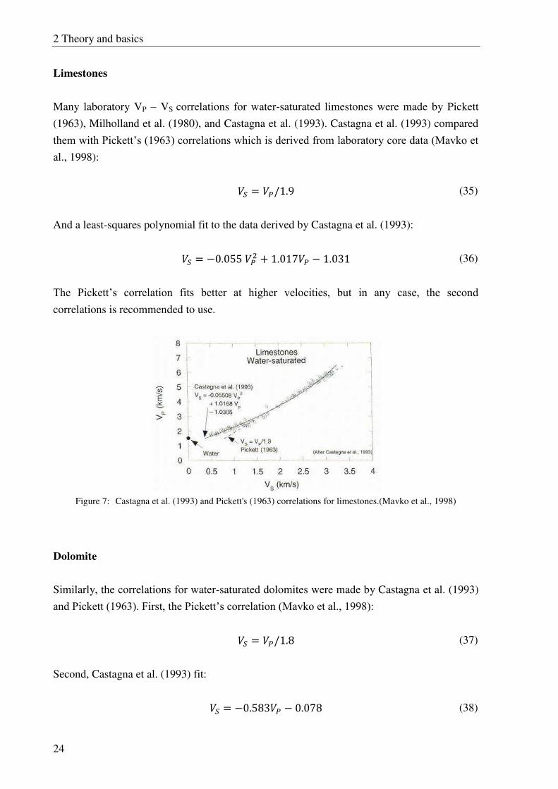
Limestones
Many laboratory VP – VS correlations for water-saturated limestones were made by Pickett
(1963), Milholland et al. (1980), and Castagna et al. (1993). Castagna et al. (1993) compared
them with Pickett’s (1963) correlations which is derived from laboratory core data (Mavko et al., 1998):
(35)
And a least-squares polynomial fit to the data derived by Castagna et al. (1993):
(36)
The Pickett’s correlation fits better at higher velocities, but in any case, the second correlations is recommended to use.
Figure 7: Castagna et al. (1993) and Pickett's (1963) correlations for limestones.(Mavko et al., 1998)
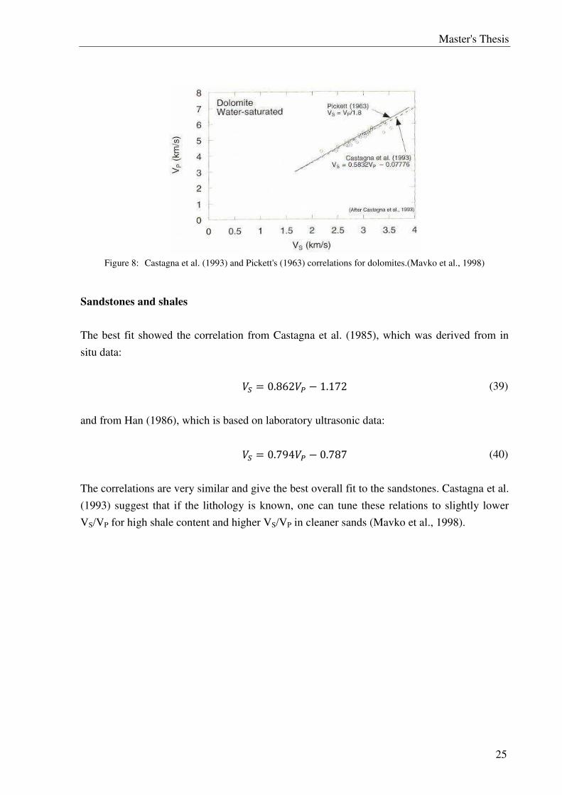
Dolomite
Similarly, the correlations for water-saturated dolomites were made by Castagna et al. (1993)
and Pickett (1963). First, the Pickett’s correlation (Mavko et al., 1998):
(37)
Second, Castagna et al. (1993) fit:
(38)
Master's Thesis
25
Figure 8: Castagna et al. (1993) and Pickett's (1963) correlations for dolomites.(Mavko et al., 1998)
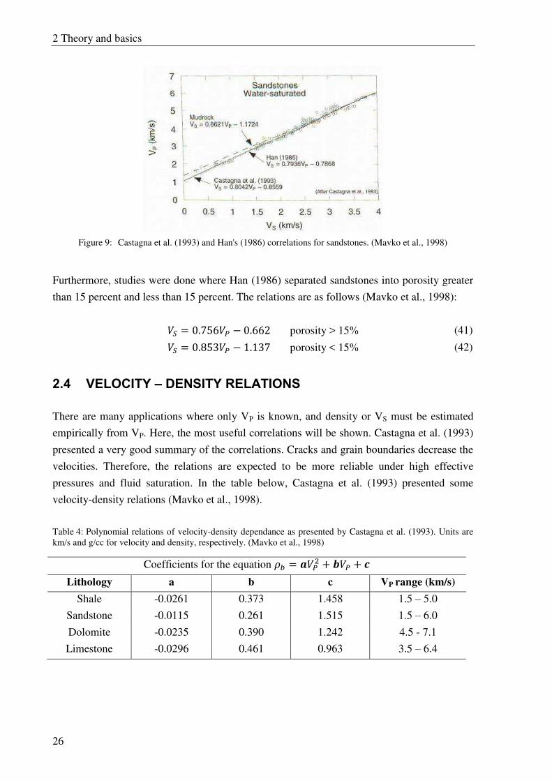
Sandstones and shales
The best fit showed the correlation from Castagna et al. (1985), which was derived from in
situ data:
(39)
and from Han (1986), which is based on laboratory ultrasonic data:
(40)
The correlations are very similar and give the best overall fit to the sandstones. Castagna et al.
(1993) suggest that if the lithology is known, one can tune these relations to slightly lower
VS/VP for high shale content and higher VS/VP in cleaner sands (Mavko et al., 1998).
2 Theory and basics
26
Figure 9: Castagna et al. (1993) and Han's (1986) correlations for sandstones. (Mavko et al., 1998)
Furthermore, studies were done where Han (1986) separated sandstones into porosity greater
than 15 percent and less than 15 percent. The relations are as follows (Mavko et al., 1998):
porosity > 15% (41)
porosity < 15% (42)
2.4 VELOCITY – DENSITY RELATIONS
There are many applications where only VP is known, and density or VS must be estimated
empirically from VP. Here, the most useful correlations will be shown. Castagna et al. (1993)
presented a very good summary of the correlations. Cracks and grain boundaries decrease the
velocities. Therefore, the relations are expected to be more reliable under high effective
pressures and fluid saturation. In the table below, Castagna et al. (1993) presented some
velocity-density relations (Mavko et al., 1998).
Table 4: Polynomial relations of velocity-density dependance as presented by Castagna et al. (1993). Units are
km/s and g/cc for velocity and density, respectively. (Mavko et al., 1998)
Coefficients for the equation
Lithology a b c VP range (km/s)
Shale -0.0261 0.373 1.458 1.5 – 5.0
Sandstone -0.0115 0.261 1.515 1.5 – 6.0
Dolomite -0.0235 0.390 1.242 4.5 - 7.1
Limestone -0.0296 0.461 0.963 3.5 – 6.4
Master's Thesis
27
2.5 LINEAR CORRELATIONS
Empirical correlations and their usage are shown in the thesis. Because these are all
correlations between two variables, it is worth describing one of the ways to correlate them.
Unfortunately, due to costly UCS test this method was not used as experimental part of the
thesis. However, the method is suggested as recommended in the discussion chapter.
As the name suggests, if two variables vary together and a relationship exists between them,
then relationship can be assumed as linear. If the relationship is positively linear, then they
both increase or decrease together. If the relationship is negatively linear, then one rises and
the other one drops. To connect two variables we basically need to fit a straight line to the
results we obtain.
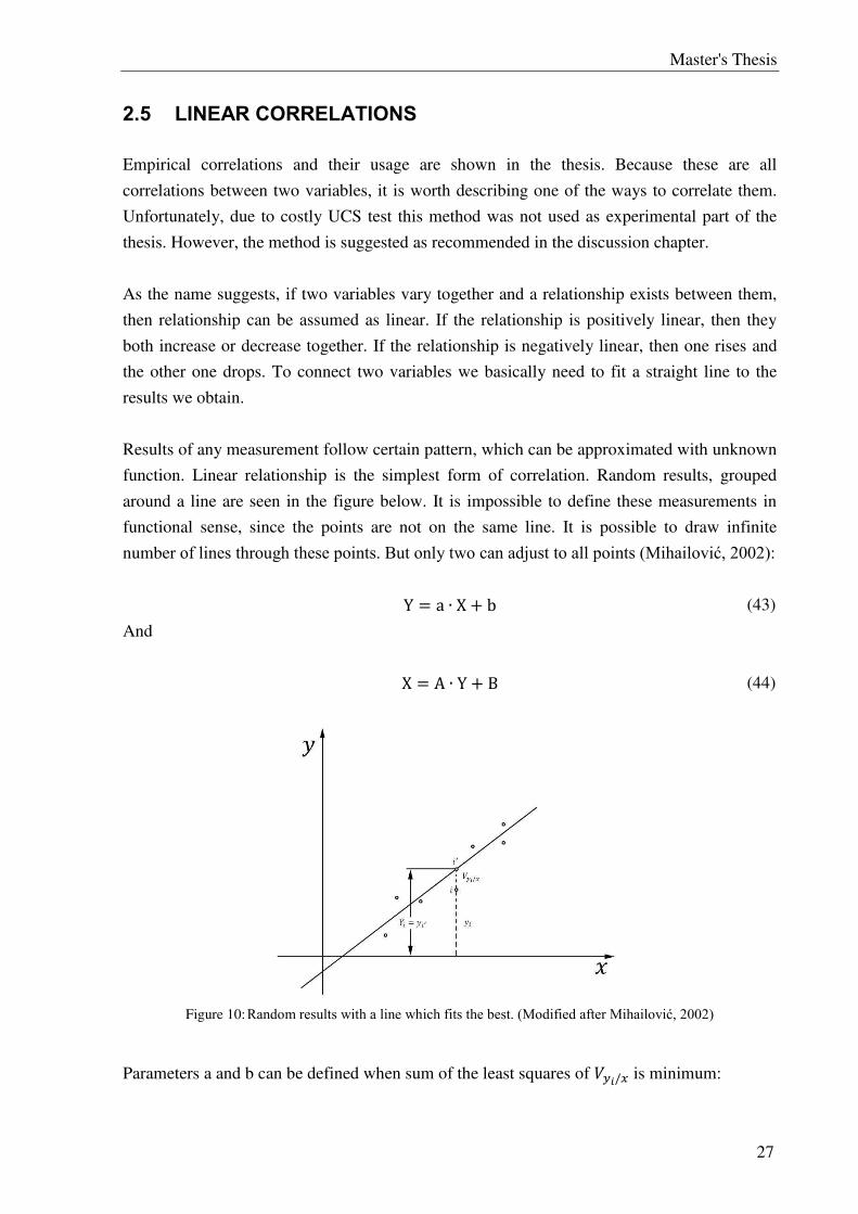
Results of any measurement follow certain pattern, which can be approximated with unknown
function. Linear relationship is the simplest form of correlation. Random results, grouped
around a line are seen in the figure below. It is impossible to define these measurements in
functional sense, since the points are not on the same line. It is possible to draw infinite
number of lines through these points. But only two can adjust to all points (Mihailović, 2002):
(43)
And
(44)
Figure 10: Random results with a line which fits the best. (Modified after Mihailović, 2002)
Parameters a and b can be defined when sum of the least squares of is minimum:

2 Theory and basics
28
, and A and B, with sum of the least squares of is minimum:
If is inserted into the equation 43, then it yields:
Because , only corrections for are made with . The system has more
known values than unknowns. Therefore, parameters a and b can be defined with the least
squares method. Parametric equations are as follows:
(45)
hence:
(46)
where and represent mean values: ,
It follows that:
( ) (47)
and
(48)
because
(49)
(50)
(51)
When the equations 45 are divided by n, then it yields:
Master's Thesis
29
(52)
and if the equation is rearranged:
(53)
Because [ ] , which follows from .
Parameter a can be derived from equation 48 and parameter b from equation 53. With these
parameters known, approximation of the real values and .
Approximation of the regression line is calculated by the following equation:
(54)
In regression analysis measured results are approximated with the line which fits these results
the best. As such, two possible cases exist. The first case, which is described above, estimates
that for already known values measures the corresponding values of , which are normally distributed ( ) The second case appears
when both values x and y and the results and follow
normal distribution and ( ) (Mihailović, 2002)
In the case of this thesis, the first case is sufficient. Ideally, we would have two sets of data;
one set about rock strengths (from the same rock, formation) and the second set would be
measured porosity or sonic velocities. X would represent the rock strength and y porosity or
second velocity, respectively. Obviously, higher number of measurements is preferred.
To make calculations easier an Add-in such as “matrix.xla” can be used in MS Excel. It has function “MCorr”, which makes the correlation in a matter of few clicks. It uses the matrix
principle and should therefore be used as matrix calculation.
3 BHA Design and drilling dynamics
30
3 BHA DESIGN AND DRILLING DYNAMICS
3.1 BHA DESIGN
BHA design is one of the most important elements while drilling a directional well. It affects
drillability, wellbore stability, hole quality and drilling direction. The BHA is the portion of
the drillsting that affects the trajectory of the bit and, consequently, of the wellbore. Its
construction could be simple, having only a drill bit, collars, and drillpipe, or it may be
complicated, having a drill bit, stabilizers, magnetic collar, telemetry unit, shock sub, collars,
reamers, jars, crossover subs, heavyweight drillpipe, and regular drillpipe. The BHA design is
dependent on many factors including, but not limited to (Buorgyne et al., 1986):
Bit side force.
Bit tilt.
Torque while drilling.
Components wear.
Riguosity of the hole (hole enlargement).
Hydraulics.
Formation dip.
Formation rock properties, especially (but not only):
o Uniaxial compression strength.
o Friction factor.
In the thesis more attention will be given to the latter two factors – effect of formation dip and
formation rock properties. Because BHA is within the formation, it is clear that BHA itself
affects the formation and that the formation reacts back on the BHA. This reaction of one on
the other will try to be analysed in details. This greatly influences the direction of the
wellbore, wear of BHA and wellbore stability including stuck pipe problems.
Master's Thesis
31
Figure 11: Typical scheme of packed and directional BHA. (Buorgyne et al., 1986)
Many other parameters are indirectly or directly affected by the formation properties, for
instance bit tilt. The tendency of the bit to build, to hold, or to drop angle is based on a
positive, zero, or negative side force. Essentially, this would be the case for hard formations
where drilling rates are below 10 ft/hr. When the formation is soft to medium-hard, the side-
fore tendency is not the only component that will influence the inclination and direction of the
bit. Because of the curvature of the BHA near the bit, the bit is canted or tilted in some
resultant direction and inclination, somewhat like the bent housing and bent sub. In such case,
the magnitude of the tilt is directly influenced by the strength of the formation. Just as a
deflection tool will not obtain the maximum curvature for which it was designed in harder
formations, so it is with a BHA a given bit tilt. For instance, in very soft formations, where
drilling rates exceeding 100 ft/hr, the side force again can be the predominant mechanism and
will, in many cases, mitigate the effects of BHA bit tilt. When the formations are soft to
medium or where drilling rates are between 10 and 100 ft/hr, effects of the bit tilt can be
significant. (Buorgyne et al., 1986)
The packed BHA and direction BHA are presented, as seen in the figure above. Packed BHA
are quite popular but they do not drill more vertical holes and they can’t drill directional holes. However, they have many advantages over other BHA types. For example, they protect
the drillpipe in the drillsting, reduce rough drilling, reduce severities of doglegs, increase drill
3 BHA Design and drilling dynamics
32
bit performance and drill straighter holes. Therefore, they are often used for drilling hold
sections. Whenever, there is a need to drill a directional well, directional BHA should be used.
The main functions of such BHA are to build the inclination, drop the inclination, walk right
or left and drill straight ahead, if needed. However, RSS motors and other techniques are used
nowadays which changes the BHA design significantly compared to ones in the past.
The formation strength and formation dip have the greatest effect on directional control of the
BHA. That is the reason why, ideally, drilling should be conducted perpendicular on the dip.
If drilling occurs in angle of attack less than 90°, then the bit will go in direction of the dip.
For optimal BHA design proper software should be used. Chen (2007) proposed software
with equilibrium dogleg severity rate prediction, force analysis, formation index calculation,
predict ahead analysis, sensitivity analysis, survey sag correction calculation and whirl
detection. The features use static and dynamic models. He claims that this is the most accurate
program in the industry. Furthermore, he verified it and compared it with other softwares in
the field which has confirmed his statement.
Figure 12: Effect of a formation dip can be observed. Additionally, perpendicular (a) and parallel (b) angle of
drilling are shown. If the angle is not perpendicular then the direction of drilling will be in the direction of a dip.
(Inglis, 1987)
BHA design must meet many specific criteria. Directional requirements, tool requirements,
hydraulics requirements, component availability, drilling optimization or operational
requirements may all have higher priority than vibration control in BHA design, but they are
all connected. (Chatar et al., 2011)
Master's Thesis
33
BHA design has a direct impact on how the drillstring responds to interaction between its
components and formation. Moreover, rock properties such as friction and rock’s strength affect both, BHA design and the BHA oscillation response. The next chapter will focus on
drilling dynamics in general and how geomechanical properties affect it.
3.2 DRILLING DYNAMICS
Drilling dynamics principles will be discussed in this chapter. The thesis focus is how
different geomechanical properties influence drilling dynamics. Before general drilling
dynamics is explained, the most important parameters should be mentioned. The uniaxial
compression strength, which is part of the experiment in the chapter 4, is the first important
property. Friction factor of tools and the wellbore is the second factor, which directly
influences vibrations. These two properties are discussed in more detail in the chapter 3.2.1.
The geomechanical knowledge about formation drilled is crucial in order to avoid or mitigate
all the severe dysfunctions which are discussed in the next paragraphs.
During drilling operations many movements occur and there are many parameters which
influence them. For any drilling operation, certain weight on bit is applied, the drillstring
rotates (except if PDM is used), the mud must be pumped, the formation acts on the
drillstring, and the drill bit is in direct contact with the formation. All these interactions affect
the bit, BHA and drillstring. The processes that are going on between these elements are
termed as drilling dynamics. As the name suggests, these are all dynamic and not static
models. Elimination of reduction of severe drilling dynamics performance may require
advanced planning and BHA design, changing operating parameters or use of a new
technology. All of these are focus of this chapter. In this chapter principles of drilling
dynamics will be researched, with a special emphasis on how different rocks affect it. Some
case studies will be shown and as a result the best practices will be given.
Firstly, the source which starts dynamic behaviour should be addressed. The most observed
one is between a rock and the bit. When the bit is on bottom it reacts with a rock in some way.
The energy which is produced between these two elements can be transferred further to the
BHA. Additionally, there are also other sources which can start excitation of the BHA, for
instance the mud pumps and the stabilizers. A stabilizer with four straight blades was found to
generate a signal at a frequency of four times RPM. For comparison, the excitation frequency
of the rock and bit interaction is of three times RPM (Burgess et al., 1987).
Secondly, some phenomena should be described. One of them is so called stick/slip
behaviour. It appears when nonlinear wellbore friction induces a torsional pendulum motion
in the BHA. The frequency of this oscillation is usually lower than the fundamental torsional
3 BHA Design and drilling dynamics
34
frequency of the BHA and it may never be noticed if there is no dynamic data. Its impact is
significant and it is an important feature of the drillstring dynamic behaviour. One way to
minimize this destructive phenomenon is to adjust surface RPM when one receives a torque
feedback (Payne, 1992). Another explanation is that this is a torsional oscillation of the BHA
while rotary drilling, where BHA stops rotating for part of its torsional cycle and then breaks
loose and rotates at high angular velocity until it stops again (Nicholson, 1994). In a situation
where stick/slip behaviour is excited because of high frequency oscillation, it can absolutely
stop the BHA (to zero RPM) and then accelerate up to 300 RPM. Such behaviour can lead to
failures (Oueslati et al., 2014).
Lateral and axial vibrations are another type of movements of the BHA. They can be caused
because of a cycle of tension and compression of the BHA components. Consequently, the
movements can induce vibration harmonics. The amplitude and frequency of these harmonics
increases with time and it produces a chaotic motion. They can often occur as shocks.
(Ramizer et al., 2010)
Another motion or phenomenon is known as the BHA whirl. It can occur when the BHA is
affected by torsional vibrations which are started because of the high rotational friction caused
by formation, for instance. Such motion can also be termed as a backward whirl. It can be
observed on the surface by the counter clockwise movement of the drillpipe around the
rathole and stalling of top drive (Ramizer et al., 2010). We distinguish between a few whirls.
First, pure forward synchronous whirl can occur, which means that drill collars whirls in the
same direction as it is rotated, and the whirl and rotary frequencies are the same. Second,
nonsynchronous forward whirl can occur, which means that the directions are the same but
the frequencies are not equal. Additionally, backward and chaotic whirl exist where chaotic
whirl means that there is neither predictable motion nor frequency. However, all whirls
involve stress cycling and therefore accelerated fatigue rates (Mason et al., 1998). Usually,
BHA whirl cannot be seen on the surface. The only indication might be a slight increase in
surface torque. Therefore, downhole tools should be used to detect increased bending moment
and lateral acceleration (JPT, 1999).
Master's Thesis
35
Figure 13: Some of the vibrations in the BHA and their possible consequences. (Ramizer et al., 2010)
Nicholson (1994) described a few natural modes of lateral vibration. When the BHA is rotated
at an angular velocity equal to a natural frequency of lateral vibration, it will bow out in its
natural mode shape while performing forward synchronous whirl. If the borehole is in gauge
and therefore lateral support is provided to the bit and stabilizers, then the drillstring can be
analysed for its natural frequencies of lateral vibration and associated mode shapes. Effects of
drillstring tension, drilling fluid buoyancy and added mass need to be included in the model.
The resulting natural frequencies are lateral vibration critical rotary speeds. Lateral vibration
critical rotary speeds are those at which the drillstring may initially perform forward
synchronous whirl which may then result in dynamic contact of the drill collar with the
borehole wall resulting in lateral shocks or backward whirl.
All these phenomena need certain excitation frequency or energy. The frequency is often
overlapping with the drilling operating frequencies, such as pump stroke, rotary speed, motor
speed, turbine, etc. The relationships can be seen in Figure 14.
Figure 14: Relationships of some known excitation frequencies to the frequencies of dynamic
behaviour.(Reckmann et al., 2010)
3 BHA Design and drilling dynamics
36
With changing only operational parameters, vibration effects may improve, but the drilling
performance can significantly decrease. If there is no extra information regarding expected
drilling dynamic behaviour, identification of the root cause of the problems may be
impossible. Therefore, the drilling dynamics problems should be addressed as a symptom of a
problem that needs to be corrected through appropriate action which, in addition to changes in
operating parameters, may include changing the drillstring and/or BHA design, changing the
bit type, installing a torque feedback control system, etc. (Nicholson, 1994)
All the effects described until now occur with low frequencies. With better technology and
methods, high frequency rotations were recorded in the field. BHA torsional vibrations and
tangential acceleration can be especially harmful. These vibrations occur at much higher
frequencies than drill collar resonance and are significantly depended on the drilled formation.
The vibrations occurred at much higher frequencies at more than 240 Hz which is more than
what was believed before. Interestingly, high frequency torsional oscillations occur at higher
WOB and low-to-moderate revolutions. This was found in a laboratory and was also
confirmed in the field. These vibrations are excited by the drilling bit and are usually not
harmful to the bit itself. However, they can excite a natural frequency of the BHA or the
whole drillstring, which can result in tool failures and NPT. (Oueslati et al., 2013 and Jain et
al., 2014).
Figure 15: WOB versus rotary speed relation and drilling dynamics dysfunctions which can occur. (Jain et al.
2014)
3.2.1 Formation effects on drilling dynamics
BHA interacts with the wellbore wall and vice versa. In the previous paragraphs, general
dynamic behaviours were described and their possible consequences were mentioned. Drilling
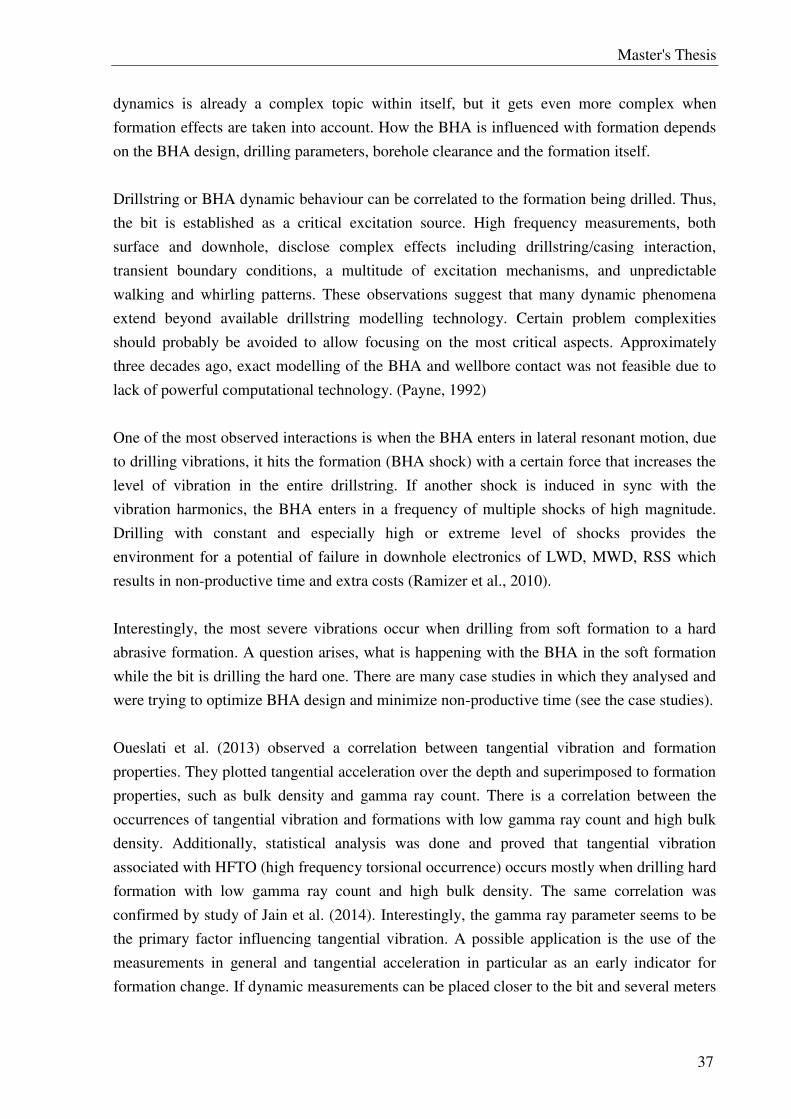
Master's Thesis
37
dynamics is already a complex topic within itself, but it gets even more complex when
formation effects are taken into account. How the BHA is influenced with formation depends
on the BHA design, drilling parameters, borehole clearance and the formation itself.
Drillstring or BHA dynamic behaviour can be correlated to the formation being drilled. Thus,
the bit is established as a critical excitation source. High frequency measurements, both
surface and downhole, disclose complex effects including drillstring/casing interaction,
transient boundary conditions, a multitude of excitation mechanisms, and unpredictable
walking and whirling patterns. These observations suggest that many dynamic phenomena
extend beyond available drillstring modelling technology. Certain problem complexities
should probably be avoided to allow focusing on the most critical aspects. Approximately
three decades ago, exact modelling of the BHA and wellbore contact was not feasible due to
lack of powerful computational technology. (Payne, 1992)
One of the most observed interactions is when the BHA enters in lateral resonant motion, due
to drilling vibrations, it hits the formation (BHA shock) with a certain force that increases the
level of vibration in the entire drillstring. If another shock is induced in sync with the
vibration harmonics, the BHA enters in a frequency of multiple shocks of high magnitude.
Drilling with constant and especially high or extreme level of shocks provides the
environment for a potential of failure in downhole electronics of LWD, MWD, RSS which
results in non-productive time and extra costs (Ramizer et al., 2010).
Interestingly, the most severe vibrations occur when drilling from soft formation to a hard
abrasive formation. A question arises, what is happening with the BHA in the soft formation
while the bit is drilling the hard one. There are many case studies in which they analysed and
were trying to optimize BHA design and minimize non-productive time (see the case studies).
Oueslati et al. (2013) observed a correlation between tangential vibration and formation
properties. They plotted tangential acceleration over the depth and superimposed to formation
properties, such as bulk density and gamma ray count. There is a correlation between the
occurrences of tangential vibration and formations with low gamma ray count and high bulk
density. Additionally, statistical analysis was done and proved that tangential vibration
associated with HFTO (high frequency torsional occurrence) occurs mostly when drilling hard
formation with low gamma ray count and high bulk density. The same correlation was
confirmed by study of Jain et al. (2014). Interestingly, the gamma ray parameter seems to be
the primary factor influencing tangential vibration. A possible application is the use of the
measurements in general and tangential acceleration in particular as an early indicator for
formation change. If dynamic measurements can be placed closer to the bit and several meters
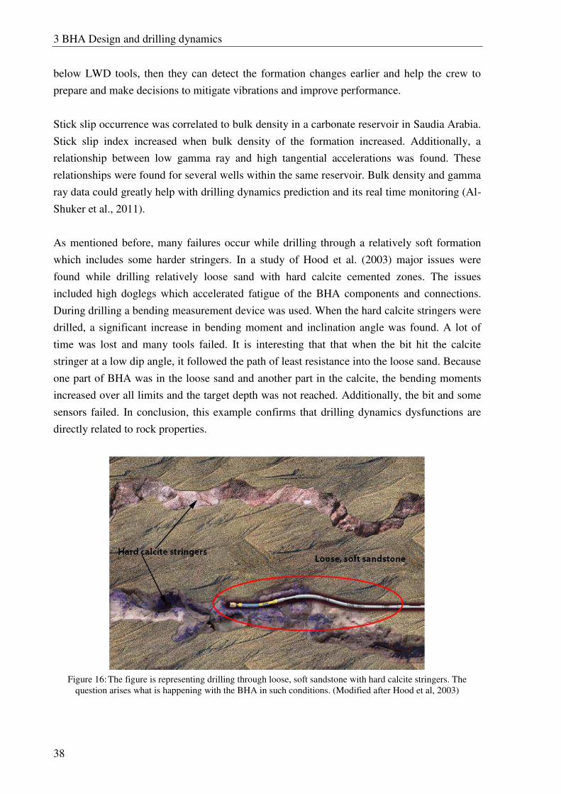
3 BHA Design and drilling dynamics
38
below LWD tools, then they can detect the formation changes earlier and help the crew to
prepare and make decisions to mitigate vibrations and improve performance.
Stick slip occurrence was correlated to bulk density in a carbonate reservoir in Saudia Arabia.
Stick slip index increased when bulk density of the formation increased. Additionally, a
relationship between low gamma ray and high tangential accelerations was found. These
relationships were found for several wells within the same reservoir. Bulk density and gamma
ray data could greatly help with drilling dynamics prediction and its real time monitoring (Al-
Shuker et al., 2011).
As mentioned before, many failures occur while drilling through a relatively soft formation
which includes some harder stringers. In a study of Hood et al. (2003) major issues were
found while drilling relatively loose sand with hard calcite cemented zones. The issues
included high doglegs which accelerated fatigue of the BHA components and connections.
During drilling a bending measurement device was used. When the hard calcite stringers were
drilled, a significant increase in bending moment and inclination angle was found. A lot of
time was lost and many tools failed. It is interesting that that when the bit hit the calcite
stringer at a low dip angle, it followed the path of least resistance into the loose sand. Because
one part of BHA was in the loose sand and another part in the calcite, the bending moments
increased over all limits and the target depth was not reached. Additionally, the bit and some
sensors failed. In conclusion, this example confirms that drilling dynamics dysfunctions are
directly related to rock properties.
Figure 16: The figure is representing drilling through loose, soft sandstone with hard calcite stringers. The
question arises what is happening with the BHA in such conditions. (Modified after Hood et al, 2003)
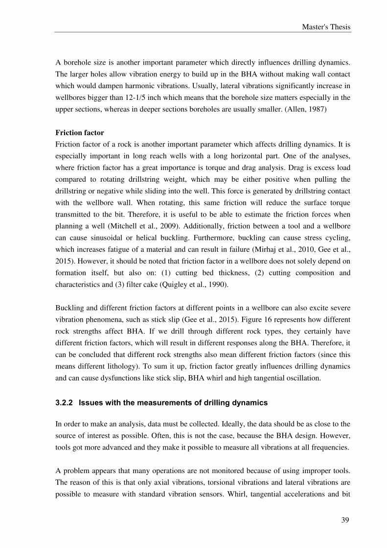
Master's Thesis
39
A borehole size is another important parameter which directly influences drilling dynamics.
The larger holes allow vibration energy to build up in the BHA without making wall contact
which would dampen harmonic vibrations. Usually, lateral vibrations significantly increase in
wellbores bigger than 12-1/5 inch which means that the borehole size matters especially in the
upper sections, whereas in deeper sections boreholes are usually smaller. (Allen, 1987)
Friction factor
Friction factor of a rock is another important parameter which affects drilling dynamics. It is
especially important in long reach wells with a long horizontal part. One of the analyses,
where friction factor has a great importance is torque and drag analysis. Drag is excess load
compared to rotating drillstring weight, which may be either positive when pulling the
drillstring or negative while sliding into the well. This force is generated by drillstring contact
with the wellbore wall. When rotating, this same friction will reduce the surface torque
transmitted to the bit. Therefore, it is useful to be able to estimate the friction forces when
planning a well (Mitchell et al., 2009). Additionally, friction between a tool and a wellbore
can cause sinusoidal or helical buckling. Furthermore, buckling can cause stress cycling,
which increases fatigue of a material and can result in failure (Mirhaj et al., 2010, Gee et al.,
2015). However, it should be noted that friction factor in a wellbore does not solely depend on
formation itself, but also on: (1) cutting bed thickness, (2) cutting composition and
characteristics and (3) filter cake (Quigley et al., 1990).
Buckling and different friction factors at different points in a wellbore can also excite severe
vibration phenomena, such as stick slip (Gee et al., 2015). Figure 16 represents how different
rock strengths affect BHA. If we drill through different rock types, they certainly have
different friction factors, which will result in different responses along the BHA. Therefore, it
can be concluded that different rock strengths also mean different friction factors (since this
means different lithology). To sum it up, friction factor greatly influences drilling dynamics
and can cause dysfunctions like stick slip, BHA whirl and high tangential oscillation.
3.2.2 Issues with the measurements of drilling dynamics
In order to make an analysis, data must be collected. Ideally, the data should be as close to the
source of interest as possible. Often, this is not the case, because the BHA design. However,
tools got more advanced and they make it possible to measure all vibrations at all frequencies.
A problem appears that many operations are not monitored because of using improper tools.
The reason of this is that only axial vibrations, torsional vibrations and lateral vibrations are
possible to measure with standard vibration sensors. Whirl, tangential accelerations and bit
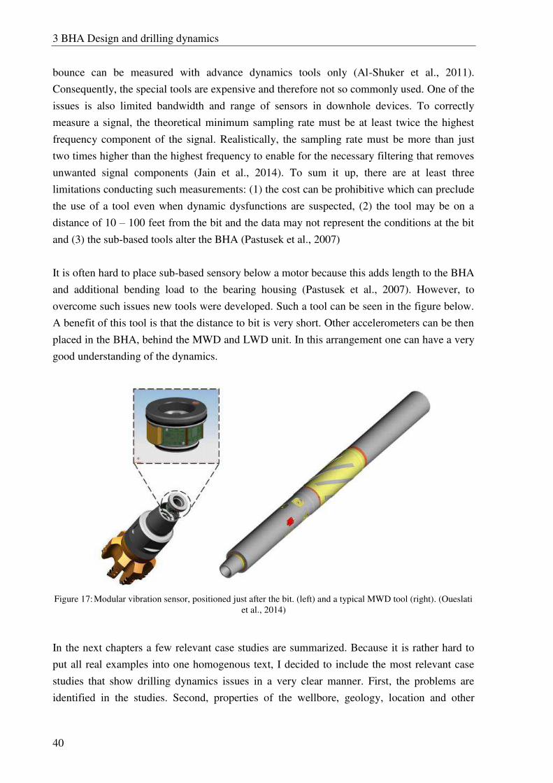
3 BHA Design and drilling dynamics
40
bounce can be measured with advance dynamics tools only (Al-Shuker et al., 2011).
Consequently, the special tools are expensive and therefore not so commonly used. One of the
issues is also limited bandwidth and range of sensors in downhole devices. To correctly
measure a signal, the theoretical minimum sampling rate must be at least twice the highest
frequency component of the signal. Realistically, the sampling rate must be more than just
two times higher than the highest frequency to enable for the necessary filtering that removes
unwanted signal components (Jain et al., 2014). To sum it up, there are at least three
limitations conducting such measurements: (1) the cost can be prohibitive which can preclude
the use of a tool even when dynamic dysfunctions are suspected, (2) the tool may be on a
distance of 10 – 100 feet from the bit and the data may not represent the conditions at the bit
and (3) the sub-based tools alter the BHA (Pastusek et al., 2007)
It is often hard to place sub-based sensory below a motor because this adds length to the BHA
and additional bending load to the bearing housing (Pastusek et al., 2007). However, to
overcome such issues new tools were developed. Such a tool can be seen in the figure below.
A benefit of this tool is that the distance to bit is very short. Other accelerometers can be then
placed in the BHA, behind the MWD and LWD unit. In this arrangement one can have a very
good understanding of the dynamics.
Figure 17: Modular vibration sensor, positioned just after the bit. (left) and a typical MWD tool (right). (Oueslati
et al., 2014)
In the next chapters a few relevant case studies are summarized. Because it is rather hard to
put all real examples into one homogenous text, I decided to include the most relevant case
studies that show drilling dynamics issues in a very clear manner. First, the problems are
identified in the studies. Second, properties of the wellbore, geology, location and other
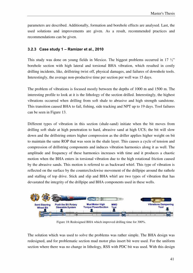
Master's Thesis
41
parameters are described. Additionally, formation and borehole effects are analysed. Last, the
used solutions and improvements are given. As a result, recommended practices and
recommendations can be given.
3.2.3 Case study 1 – Ramizer et al., 2010
This study was done on young fields in Mexico. The biggest problems occurred in 17 ½” borehole section with high lateral and torsional BHA vibration, which resulted in costly
drilling incidents, like, drillstring twist off, physical damages, and failures of downhole tools.
Interestingly, the average non-productive time per section per well was 15 days.
The problem of vibrations is focused mostly between the depths of 1000 m and 1500 m. The
interesting profile to look at it is the lithology of the section drilled. Interestingly, the highest
vibrations occurred when drilling from soft shale to abrasive and high strength sandstone.
This transition caused BHA to fail, fishing, side tracking and NPT up to 19 days. Tool failures
can be seen in Figure 13.
Different types of vibration in this section (shale-sand) initiate when the bit moves from
drilling soft shale at high penetration to hard, abrasive sand at high UCS; the bit will slow
down and the drillstring enters higher compression as the driller applies higher weight on bit
to maintain the same ROP that was seen in the shale layer. This causes a cycle of tension and
compression of drillstring components and induces vibration harmonics along it as well. The
amplitude and frequency of these harmonics increases with time and it produces a chaotic
motion when the BHA enters in torsional vibration due to the high rotational friction caused
by the abrasive sands. This motion is referred to as backward whirl. This type of vibration is
reflected on the surface by the counterclockwise movement of the drillpipe around the rathole
and stalling of top drive. Stick and slip and BHA whirl are two types of vibration that has
devastated the integrity of the drillpipe and BHA components used in these wells.
Figure 18: Redesigned BHA which improved drilling time for 300%.
The solution which was used to solve the problems was rather simple. The BHA design was
redesigned, and for problematic section mud motor plus insert bit were used. For the uniform
section where there was no change in lithology, RSS with PDC bit was used. With this design
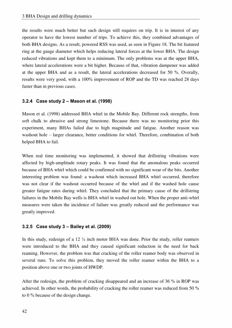
3 BHA Design and drilling dynamics
42
the results were much better but such design still requires on trip. It is in interest of any
operator to have the lowest number of trips. To achieve this, they combined advantages of
both BHA designs. As a result, powered RSS was used, as seen in Figure 18. The bit featured
ring at the gauge diameter which helps reducing lateral forces at the lower BHA. The design
reduced vibrations and kept them to a minimum. The only problems was at the upper BHA,
where lateral accelerations were a bit higher. Because of that, vibration dampener was added
at the upper BHA and as a result, the lateral accelerations decreased for 50 %. Overally,
results were very good, with a 100% improvement of ROP and the TD was reached 28 days
faster than in previous cases.
3.2.4 Case study 2 – Mason et al. (1998)
Mason et al. (1998) addressed BHA whirl in the Mobile Bay. Different rock strengths, from
soft chalk to abrasive and strong limestone. Because there was no monitoring prior this
experiment, many BHAs failed due to high magnitude and fatigue. Another reason was
washout hole – larger clearance, better conditions for whirl. Therefore, combination of both
helped BHA to fail.
When real time monitoring was implemented, it showed that drillstring vibrations were
affected by high-amplitude rotary peaks. It was found that the anomalous peaks occurred
because of BHA whirl which could be confirmed with no significant wear of the bits. Another
interesting problem was found: a washout which increased BHA whirl occurred, therefore
was not clear if the washout occurred because of the whirl and if the washed hole cause
greater fatigue rates during whirl. They concluded that the primary cause of the drillstring
failures in the Mobile Bay wells is BHA whirl in washed out hole. When the proper anti-whirl
measures were taken the incidence of failure was greatly reduced and the performance was
greatly improved.
3.2.5 Case study 3 – Bailey et al. (2009)
In this study, redesign of a 12 ¼ inch motor BHA was done. Prior the study, roller reamers were introduced to the BHA and they caused significant reduction in the need for back
reaming. However, the problem was that cracking of the roller reamer body was observed in
several runs. To solve this problem, they moved the roller reamer within the BHA to a
position above one or two joints of HWDP.
After the redesign, the problem of cracking disappeared and an increase of 36 % in ROP was
achieved. In other words, the probability of cracking the roller reamer was reduced from 50 %
to 0 % because of the design change.
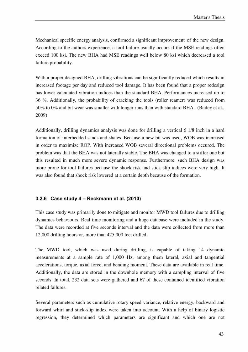
Master's Thesis
43
Mechanical specific energy analysis, confirmed a significant improvement of the new design.
According to the authors experience, a tool failure usually occurs if the MSE readings often
exceed 100 ksi. The new BHA had MSE readings well below 80 ksi which decreased a tool
failure probability.
With a proper designed BHA, drilling vibrations can be significantly reduced which results in
increased footage per day and reduced tool damage. It has been found that a proper redesign
has lower calculated vibration indices than the standard BHA. Performances increased up to
36 %. Additionally, the probability of cracking the tools (roller reamer) was reduced from
50% to 0% and bit wear was smaller with longer runs than with standard BHA. (Bailey et al.,
2009)
Additionally, drilling dynamics analysis was done for drilling a vertical 6 1/8 inch in a hard
formation of interbedded sands and shales. Because a new bit was used, WOB was increased
in order to maximize ROP. With increased WOB several directional problems occured. The
problem was that the BHA was not laterally stable. The BHA was changed to a stiffer one but
this resulted in much more severe dynamic response. Furthermore, such BHA design was
more prone for tool failures because the shock risk and stick-slip indices were very high. It
was also found that shock risk lowered at a certain depth because of the formation.
3.2.6 Case study 4 – Reckmann et al. (2010)
This case study was primarily done to mitigate and monitor MWD tool failures due to drilling
dynamics behaviours. Real time monitoring and a huge database were included in the study.
The data were recorded at five seconds interval and the data were collected from more than
12,000 drilling hours or, more than 425,000 feet drilled.
The MWD tool, which was used during drilling, is capable of taking 14 dynamic
measurements at a sample rate of 1,000 Hz, among them lateral, axial and tangential
accelerations, torque, axial force, and bending moment. These data are available in real time.
Additionally, the data are stored in the downhole memory with a sampling interval of five
seconds. In total, 232 data sets were gathered and 67 of these contained identified vibration
related failures.
Several parameters such as cumulative rotary speed variance, relative energy, backward and
forward whirl and stick-slip index were taken into account. With a help of binary logistic
regression, they determined which parameters are significant and which one are not
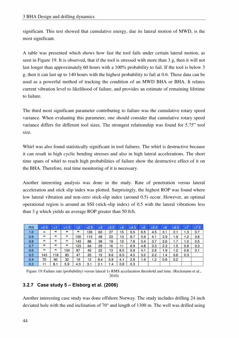
3 BHA Design and drilling dynamics
44
significant. This test showed that cumulative energy, due its lateral motion of MWD, is the
most significant.
A table was presented which shows how fast the tool fails under certain lateral motion, as
seen in Figure 19. It is observed, that if the tool is stressed with more than 3 g, then it will not
last longer than approximately 60 hours with a 100% probability to fail. If the tool is below 3
g, then it can last up to 140 hours with the highest probability to fail at 0.6. These data can be
used as a powerful method of tracking the condition of an MWD BHA or BHA. It relates
current vibration level to likelihood of failure, and provides an estimate of remaining lifetime
to failure.
The third most significant parameter contributing to failure was the cumulative rotary speed
variance. When evaluating this parameter, one should consider that cumulative rotary speed
variance differs for different tool sizes. The strongest relationship was found for 5.75” tool size.
Whirl was also found statistically significant in tool failures. The whirl is destructive because
it can result in high cyclic bending stresses and also in high lateral accelerations. The short
time spans of whirl to reach high probabilities of failure show the destructive effect of it on
the BHA. Therefore, real time monitoring of it is necessary.
Another interesting analysis was done in the study. Rate of penetration versus lateral
acceleration and stick slip index was plotted. Surprisingly, the highest ROP was found where
low lateral vibration and non-zero stick-slip index (around 0.5) occur. However, an optimal
operational region is around an SSI (stick-slip index) of 0.5 with the lateral vibrations less
than 3 g which yields an average ROP greater than 50 ft/h.
Figure 19: Failure rate (probability) versus lateral 1s RMS accelaration threshold and time. (Reckmann et al.,
2010)
3.2.7 Case study 5 – Elsborg et al. (2006)
Another interesting case study was done offshore Norway. The study includes drilling 24 inch
deviated hole with the end inclination of 70° and length of 1300 m. The well was drilled using
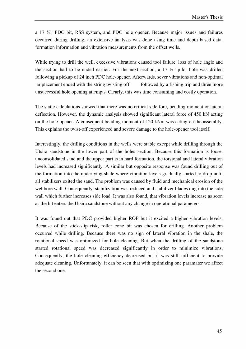
Master's Thesis
45
a 17 ½” PDC bit, RSS system, and PDC hole opener. Because major issues and failures
occurred during drilling, an extensive analysis was done using time and depth based data,
formation information and vibration measurements from the offset wells.
While trying to drill the well, excessive vibrations caused tool failure, loss of hole angle and
the section had to be ended earlier. For the next section, a 17 ½” pilot hole was drilled following a pickup of 24 inch PDC hole-opener. Afterwards, sever vibrations and non-optimal
jar placement ended with the string twisting off followed by a fishing trip and three more
unsuccessful hole opening attempts. Clearly, this was time consuming and costly operation.
The static calculations showed that there was no critical side fore, bending moment or lateral
deflection. However, the dynamic analysis showed significant lateral force of 450 kN acting
on the hole-opener. A consequent bending moment of 120 kNm was acting on the assembly.
This explains the twist-off experienced and severe damage to the hole-opener tool itself.
Interestingly, the drilling conditions in the wells were stable except while drilling through the
Utsira sandstone in the lower part of the holes section. Because this formation is loose,
unconsolidated sand and the upper part is in hard formation, the torsional and lateral vibration
levels had increased significantly. A similar but opposite response was found drilling out of
the formation into the underlying shale where vibration levels gradually started to drop until
all stabilizers exited the sand. The problem was caused by fluid and mechanical erosion of the
wellbore wall. Consequently, stabilization was reduced and stabilizer blades dug into the side
wall which further increases side load. It was also found, that vibration levels increase as soon
as the bit enters the Utsira sandstone without any change in operational parameters.
It was found out that PDC provided higher ROP but it excited a higher vibration levels.
Because of the stick-slip risk, roller cone bit was chosen for drilling. Another problem
occurred while drilling. Because there was no sign of lateral vibration in the shale, the
rotational speed was optimized for hole cleaning. But when the drilling of the sandstone
started rotational speed was decreased significantly in order to minimize vibrations.
Consequently, the hole cleaning efficiency decreased but it was still sufficient to provide
adequate cleaning. Unfortunately, it can be seen that with optimizing one paramater we affect
the second one.
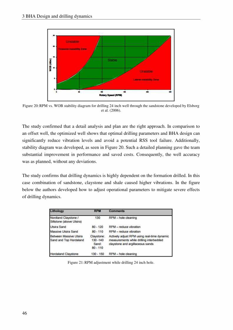
3 BHA Design and drilling dynamics
46
Figure 20: RPM vs. WOB stability diagram for drilling 24 inch well through the sandstone developed by Elsborg
et al. (2006).
The study confirmed that a detail analysis and plan are the right approach. In comparison to
an offset well, the optimized well shows that optimal drilling parameters and BHA design can
significantly reduce vibration levels and avoid a potential RSS tool failure. Additionally,
stability diagram was developed, as seen in Figure 20. Such a detailed planning gave the team
substantial improvement in performance and saved costs. Consequently, the well accuracy
was as planned, without any deviations.
The study confirms that drilling dynamics is highly dependent on the formation drilled. In this
case combination of sandstone, claystone and shale caused higher vibrations. In the figure
below the authors developed how to adjust operational parameters to mitigate severe effects
of drilling dynamics.
Figure 21: RPM adjustment while drilling 24 inch hole.
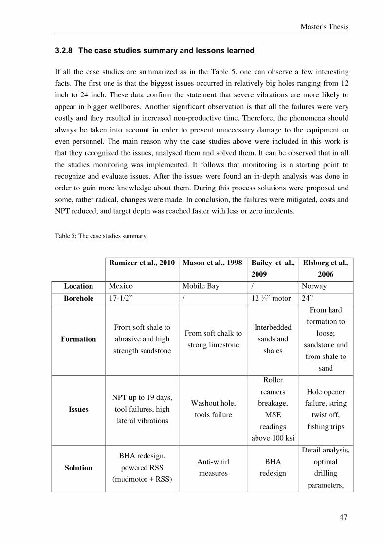
Master's Thesis
47
3.2.8 The case studies summary and lessons learned
If all the case studies are summarized as in the Table 5, one can observe a few interesting
facts. The first one is that the biggest issues occurred in relatively big holes ranging from 12
inch to 24 inch. These data confirm the statement that severe vibrations are more likely to
appear in bigger wellbores. Another significant observation is that all the failures were very
costly and they resulted in increased non-productive time. Therefore, the phenomena should
always be taken into account in order to prevent unnecessary damage to the equipment or
even personnel. The main reason why the case studies above were included in this work is
that they recognized the issues, analysed them and solved them. It can be observed that in all
the studies monitoring was implemented. It follows that monitoring is a starting point to
recognize and evaluate issues. After the issues were found an in-depth analysis was done in
order to gain more knowledge about them. During this process solutions were proposed and
some, rather radical, changes were made. In conclusion, the failures were mitigated, costs and
NPT reduced, and target depth was reached faster with less or zero incidents.
Table 5: The case studies summary.
Ramizer et al., 2010 Mason et al., 1998 Bailey et al.,
2009
Elsborg et al.,
2006
Location Mexico Mobile Bay / Norway
Borehole 17-1/2” / 12 ¼” motor 24”
Formation
From soft shale to
abrasive and high
strength sandstone
From soft chalk to
strong limestone
Interbedded
sands and
shales
From hard
formation to
loose;
sandstone and
from shale to
sand
Issues
NPT up to 19 days,
tool failures, high
lateral vibrations
Washout hole,
tools failure
Roller
reamers
breakage,
MSE
readings
above 100 ksi
Hole opener
failure, string
twist off,
fishing trips
Solution
BHA redesign,
powered RSS
(mudmotor + RSS)
Anti-whirl
measures
BHA
redesign
Detail analysis,
optimal
drilling
parameters,

3 BHA Design and drilling dynamics
48
BHA redesign.
Improvement
100% ROP
improvement
Lat. Acc. Decreased
50%
TD reached 28 days
faster
Failure rate
dramatically
reduced
Cracking
reduced to 0.
36% ROP
increase
Accurate,
reduced
vibrations, no
tool failures.
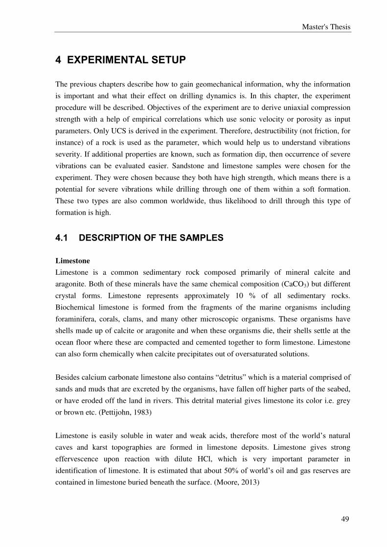
Master's Thesis
49
4 EXPERIMENTAL SETUP
The previous chapters describe how to gain geomechanical information, why the information
is important and what their effect on drilling dynamics is. In this chapter, the experiment
procedure will be described. Objectives of the experiment are to derive uniaxial compression
strength with a help of empirical correlations which use sonic velocity or porosity as input
parameters. Only UCS is derived in the experiment. Therefore, destructibility (not friction, for
instance) of a rock is used as the parameter, which would help us to understand vibrations
severity. If additional properties are known, such as formation dip, then occurrence of severe
vibrations can be evaluated easier. Sandstone and limestone samples were chosen for the
experiment. They were chosen because they both have high strength, which means there is a
potential for severe vibrations while drilling through one of them within a soft formation.
These two types are also common worldwide, thus likelihood to drill through this type of
formation is high.
4.1 DESCRIPTION OF THE SAMPLES
Limestone
Limestone is a common sedimentary rock composed primarily of mineral calcite and
aragonite. Both of these minerals have the same chemical composition (CaCO3) but different
crystal forms. Limestone represents approximately 10 % of all sedimentary rocks.
Biochemical limestone is formed from the fragments of the marine organisms including
foraminifera, corals, clams, and many other microscopic organisms. These organisms have
shells made up of calcite or aragonite and when these organisms die, their shells settle at the
ocean floor where these are compacted and cemented together to form limestone. Limestone
can also form chemically when calcite precipitates out of oversaturated solutions.
Besides calcium carbonate limestone also contains “detritus” which is a material comprised of sands and muds that are excreted by the organisms, have fallen off higher parts of the seabed,
or have eroded off the land in rivers. This detrital material gives limestone its color i.e. grey
or brown etc. (Pettijohn, 1983)
Limestone is easily soluble in water and weak acids, therefore most of the world’s natural caves and karst topographies are formed in limestone deposits. Limestone gives strong
effervescence upon reaction with dilute HCl, which is very important parameter in
identification of limestone. It is estimated that about 50% of world’s oil and gas reserves are contained in limestone buried beneath the surface. (Moore, 2013)
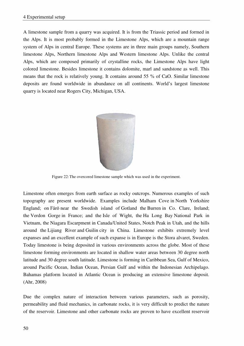
4 Experimental setup
50
A limestone sample from a quarry was acquired. It is from the Triassic period and formed in
the Alps. It is most probably formed in the Limestone Alps, which are a mountain range
system of Alps in central Europe. These systems are in three main groups namely, Southern
limestone Alps, Northern limestone Alps and Western limestone Alps. Unlike the central
Alps, which are composed primarily of crystalline rocks, the Limestone Alps have light
colored limestone. Besides limestone it contains dolomite, marl and sandstone as well. This
means that the rock is relatively young. It contains around 55 % of CaO. Similar limestone
deposits are found worldwide in abundance on all continents. World’s largest limestone quarry is located near Rogers City, Michigan, USA.
Figure 22: The overcored limestone sample which was used in the experiment.
Limestone often emerges from earth surface as rocky outcrops. Numerous examples of such
topography are present worldwide. Examples include Malham Cove in North Yorkshire
England; on Fårö near the Swedish island of Gotland the Burren in Co. Clare, Ireland;
the Verdon Gorge in France; and the Isle of Wight, the Ha Long Bay National Park in
Vietnam, the Niagara Escarpment in Canada/United States, Notch Peak in Utah, and the hills
around the Lijiang River and Guilin city in China. Limestone exhibits extremely level
expanses and an excellent example of such expanse is in Europe is the Stora alvaret, Sweden.
Today limestone is being deposited in various environments across the globe. Most of these
limestone forming environments are located in shallow water areas between 30 degree north
latitude and 30 degree south latitude. Limestone is forming in Caribbean Sea, Gulf of Mexico,
around Pacific Ocean, Indian Ocean, Persian Gulf and within the Indonesian Archipelago.
Bahamas platform located in Atlantic Ocean is producing an extensive limestone deposit.
(Ahr, 2008)
Due the complex nature of interaction between various parameters, such as porosity,
permeability and fluid mechanics, in carbonate rocks, it is very difficult to predict the nature
of the reservoir. Limestone and other carbonate rocks are proven to have excellent reservoir
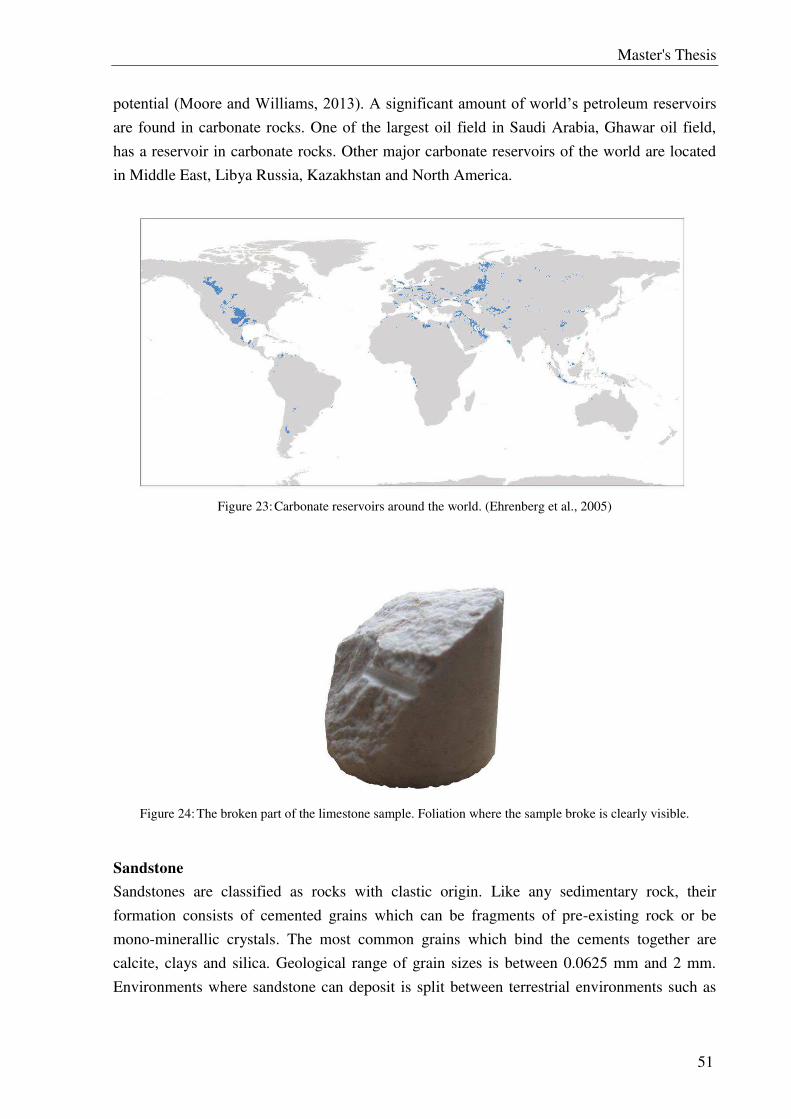
Master's Thesis
51
potential (Moore and Williams, 2013). A significant amount of world’s petroleum reservoirs
are found in carbonate rocks. One of the largest oil field in Saudi Arabia, Ghawar oil field,
has a reservoir in carbonate rocks. Other major carbonate reservoirs of the world are located
in Middle East, Libya Russia, Kazakhstan and North America.
Figure 23: Carbonate reservoirs around the world. (Ehrenberg et al., 2005)
Figure 24: The broken part of the limestone sample. Foliation where the sample broke is clearly visible.
Sandstone
Sandstones are classified as rocks with clastic origin. Like any sedimentary rock, their
formation consists of cemented grains which can be fragments of pre-existing rock or be
mono-minerallic crystals. The most common grains which bind the cements together are
calcite, clays and silica. Geological range of grain sizes is between 0.0625 mm and 2 mm.
Environments where sandstone can deposit is split between terrestrial environments such as
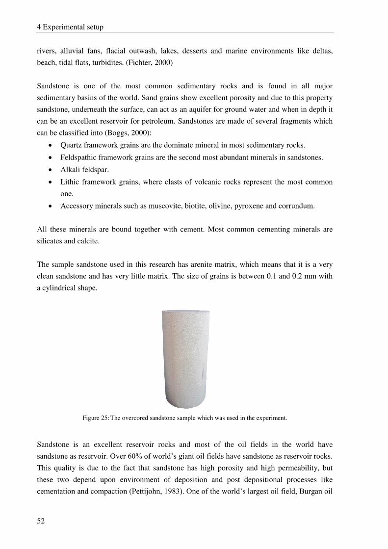
4 Experimental setup
52
rivers, alluvial fans, flacial outwash, lakes, desserts and marine environments like deltas,
beach, tidal flats, turbidites. (Fichter, 2000)
Sandstone is one of the most common sedimentary rocks and is found in all major
sedimentary basins of the world. Sand grains show excellent porosity and due to this property
sandstone, underneath the surface, can act as an aquifer for ground water and when in depth it
can be an excellent reservoir for petroleum. Sandstones are made of several fragments which
can be classified into (Boggs, 2000):
Quartz framework grains are the dominate mineral in most sedimentary rocks.
Feldspathic framework grains are the second most abundant minerals in sandstones.
Alkali feldspar.
Lithic framework grains, where clasts of volcanic rocks represent the most common
one.
Accessory minerals such as muscovite, biotite, olivine, pyroxene and corrundum.
All these minerals are bound together with cement. Most common cementing minerals are
silicates and calcite.
The sample sandstone used in this research has arenite matrix, which means that it is a very
clean sandstone and has very little matrix. The size of grains is between 0.1 and 0.2 mm with
a cylindrical shape.
Figure 25: The overcored sandstone sample which was used in the experiment.
Sandstone is an excellent reservoir rocks and most of the oil fields in the world have
sandstone as reservoir. Over 60% of world’s giant oil fields have sandstone as reservoir rocks. This quality is due to the fact that sandstone has high porosity and high permeability, but
these two depend upon environment of deposition and post depositional processes like
cementation and compaction (Pettijohn, 1983). One of the world’s largest oil field, Burgan oil
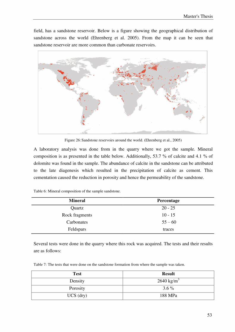
Master's Thesis
53
field, has a sandstone reservoir. Below is a figure showing the geographical distribution of
sandstone across the world (Ehrenberg et al. 2005). From the map it can be seen that
sandstone reservoir are more common than carbonate reservoirs.
Figure 26: Sandstone reservoirs around the world. (Ehrenberg et al., 2005)
A laboratory analysis was done from in the quarry where we got the sample. Mineral
composition is as presented in the table below. Additionally, 53.7 % of calcite and 4.1 % of
dolomite was found in the sample. The abundance of calcite in the sandstone can be attributed
to the late diagenesis which resulted in the precipitation of calcite as cement. This
cementation caused the reduction in porosity and hence the permeability of the sandstone.
Table 6: Mineral composition of the sample sandstone.
Mineral Percentage
Quartz 20 - 25
Rock fragments 10 - 15
Carbonates 55 – 60
Feldspars traces
Several tests were done in the quarry where this rock was acquired. The tests and their results
are as follows:
Table 7: The tests that were done on the sandstone formation from where the sample was taken.
Test Result
Density 2640 kg/m3
Porosity 3.6 %
UCS (dry) 188 MPa
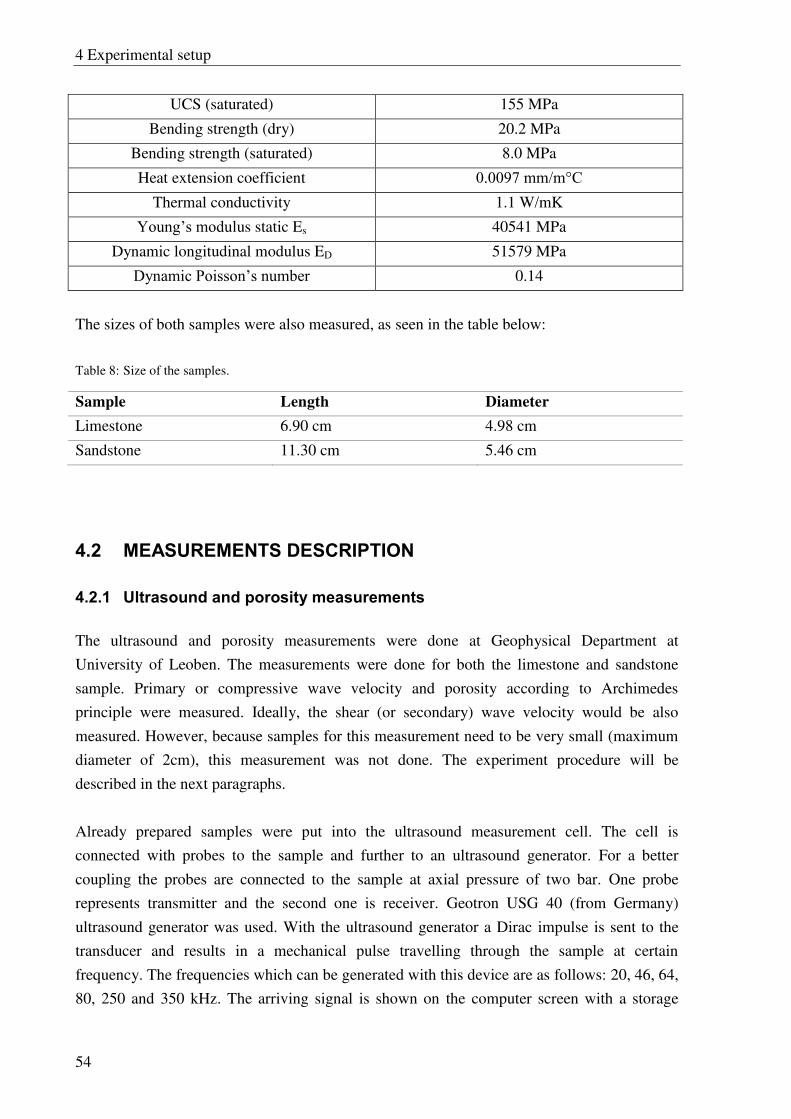
4 Experimental setup
54
UCS (saturated) 155 MPa
Bending strength (dry) 20.2 MPa
Bending strength (saturated) 8.0 MPa
Heat extension coefficient 0.0097 mm/m°C
Thermal conductivity 1.1 W/mK
Young’s modulus static Es 40541 MPa
Dynamic longitudinal modulus ED 51579 MPa
Dynamic Poisson’s number 0.14
The sizes of both samples were also measured, as seen in the table below:
Table 8: Size of the samples.
Sample Length Diameter
Limestone 6.90 cm 4.98 cm
Sandstone 11.30 cm 5.46 cm
4.2 MEASUREMENTS DESCRIPTION
4.2.1 Ultrasound and porosity measurements
The ultrasound and porosity measurements were done at Geophysical Department at
University of Leoben. The measurements were done for both the limestone and sandstone
sample. Primary or compressive wave velocity and porosity according to Archimedes
principle were measured. Ideally, the shear (or secondary) wave velocity would be also
measured. However, because samples for this measurement need to be very small (maximum
diameter of 2cm), this measurement was not done. The experiment procedure will be
described in the next paragraphs.
Already prepared samples were put into the ultrasound measurement cell. The cell is
connected with probes to the sample and further to an ultrasound generator. For a better
coupling the probes are connected to the sample at axial pressure of two bar. One probe
represents transmitter and the second one is receiver. Geotron USG 40 (from Germany)
ultrasound generator was used. With the ultrasound generator a Dirac impulse is sent to the
transducer and results in a mechanical pulse travelling through the sample at certain
frequency. The frequencies which can be generated with this device are as follows: 20, 46, 64,
80, 250 and 350 kHz. The arriving signal is shown on the computer screen with a storage
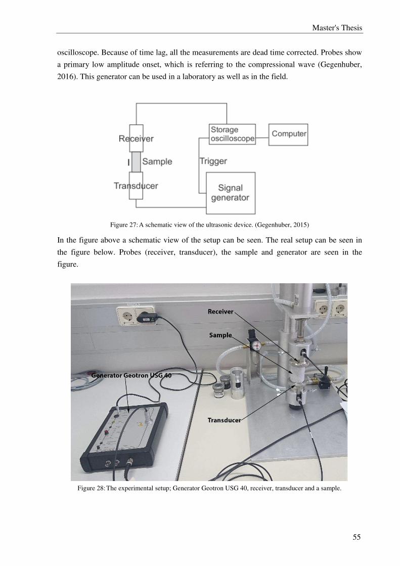
Master's Thesis
55
oscilloscope. Because of time lag, all the measurements are dead time corrected. Probes show
a primary low amplitude onset, which is referring to the compressional wave (Gegenhuber,
2016). This generator can be used in a laboratory as well as in the field.
Figure 27: A schematic view of the ultrasonic device. (Gegenhuber, 2015)
In the figure above a schematic view of the setup can be seen. The real setup can be seen in
the figure below. Probes (receiver, transducer), the sample and generator are seen in the
figure.
Figure 28: The experimental setup; Generator Geotron USG 40, receiver, transducer and a sample.
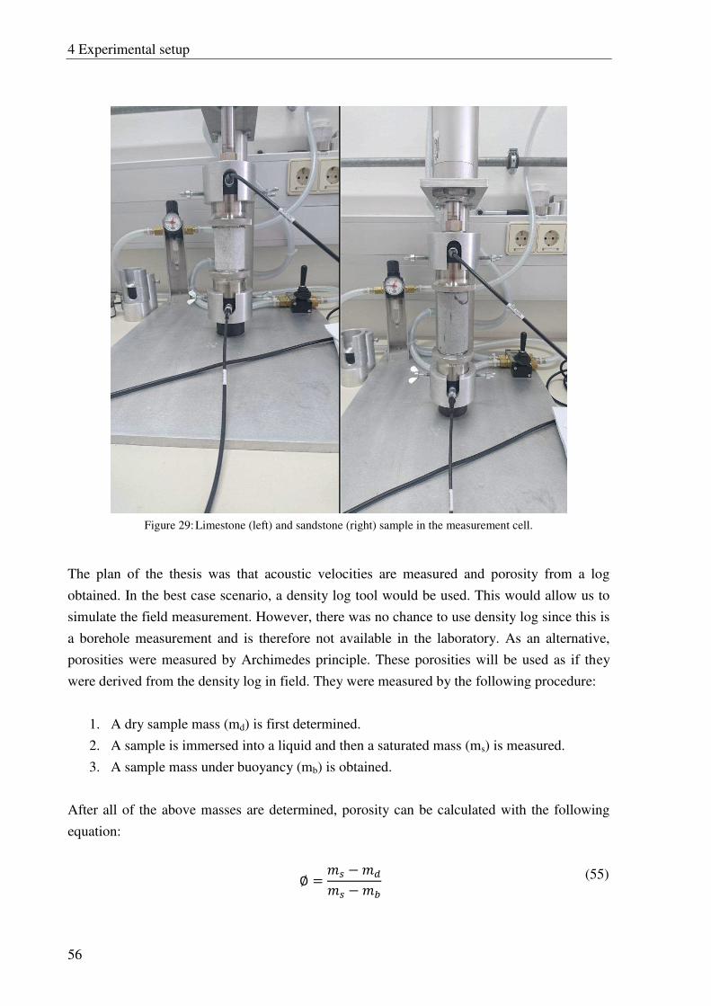
4 Experimental setup
56
Figure 29: Limestone (left) and sandstone (right) sample in the measurement cell.
The plan of the thesis was that acoustic velocities are measured and porosity from a log
obtained. In the best case scenario, a density log tool would be used. This would allow us to
simulate the field measurement. However, there was no chance to use density log since this is
a borehole measurement and is therefore not available in the laboratory. As an alternative,
porosities were measured by Archimedes principle. These porosities will be used as if they
were derived from the density log in field. They were measured by the following procedure:
1. A dry sample mass (md) is first determined.
2. A sample is immersed into a liquid and then a saturated mass (ms) is measured.
3. A sample mass under buoyancy (mb) is obtained.
After all of the above masses are determined, porosity can be calculated with the following
equation:
(55)
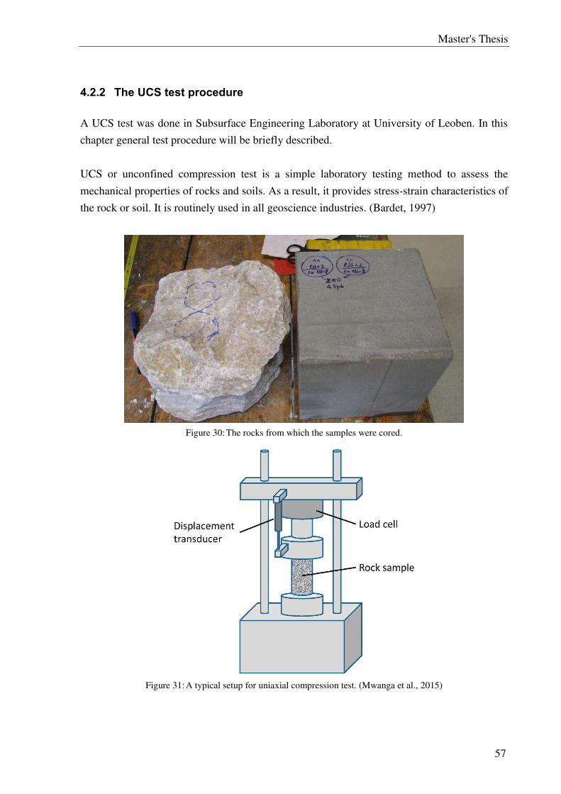
Master's Thesis
57
4.2.2 The UCS test procedure
A UCS test was done in Subsurface Engineering Laboratory at University of Leoben. In this
chapter general test procedure will be briefly described.
UCS or unconfined compression test is a simple laboratory testing method to assess the
mechanical properties of rocks and soils. As a result, it provides stress-strain characteristics of
the rock or soil. It is routinely used in all geoscience industries. (Bardet, 1997)
Figure 30: The rocks from which the samples were cored.
Figure 31: A typical setup for uniaxial compression test. (Mwanga et al., 2015)
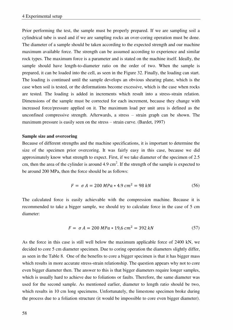
4 Experimental setup
58
Prior performing the test, the sample must be properly prepared. If we are sampling soil a
cylindrical tube is used and if we are sampling rocks an over-coring operation must be done.
The diameter of a sample should be taken according to the expected strength and our machine
maximum available force. The strength can be assumed according to experience and similar
rock types. The maximum force is a parameter and is stated on the machine itself. Ideally, the
sample should have length-to-diameter ratio on the order of two. When the sample is
prepared, it can be loaded into the cell, as seen in the Figure 32. Finally, the loading can start.
The loading is continued until the sample develops an obvious shearing plane, which is the
case when soil is tested, or the deformations become excessive, which is the case when rocks
are tested. The loading is added in increments which result into a stress-strain relation.
Dimensions of the sample must be corrected for each increment, because they change with
increased force/pressure applied on it. The maximum load per unit area is defined as the
unconfined compressive strength. Afterwards, a stress – strain graph can be shown. The
maximum pressure is easily seen on the stress – strain curve. (Bardet, 1997)
Sample size and overcoring
Because of different strengths and the machine specifications, it is important to determine the
size of the specimen prior overcoring. It was fairly easy in this case, because we did
approximately know what strength to expect. First, if we take diameter of the specimen of 2.5
cm, then the area of the cylinder is around 4.9 cm2. If the strength of the sample is expected to
be around 200 MPa, then the force should be as follows:
(56)
The calculated force is easily achievable with the compression machine. Because it is
recommended to take a bigger sample, we should try to calculate force in the case of 5 cm
diameter:
(57)
As the force in this case is still well below the maximum applicable force of 2400 kN, we
decided to core 5 cm diameter specimen. Due to coring operation the diameters slightly differ,
as seen in the Table 8. One of the benefits to core a bigger specimen is that it has bigger mass
which results in more accurate stress-strain relationship. The question appears why not to core
even bigger diameter then. The answer to this is that bigger diameters require longer samples,
which is usually hard to achieve due to foliations or faults. Therefore, the same diameter was
used for the second sample. As mentioned earlier, diameter to length ratio should be two,
which results in 10 cm long specimens. Unfortunately, the limestone specimen broke during
the process due to a foliation structure (it would be impossible to core even bigger diameter).
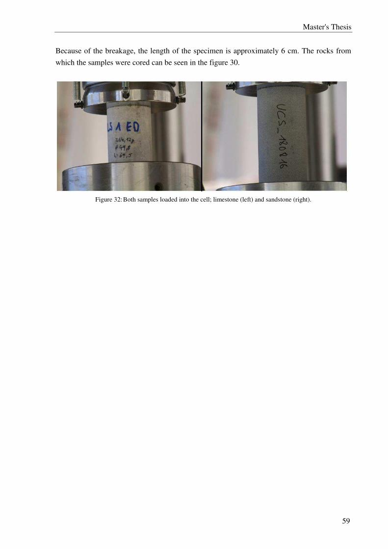
Master's Thesis
59
Because of the breakage, the length of the specimen is approximately 6 cm. The rocks from
which the samples were cored can be seen in the figure 30.
Figure 32: Both samples loaded into the cell; limestone (left) and sandstone (right).
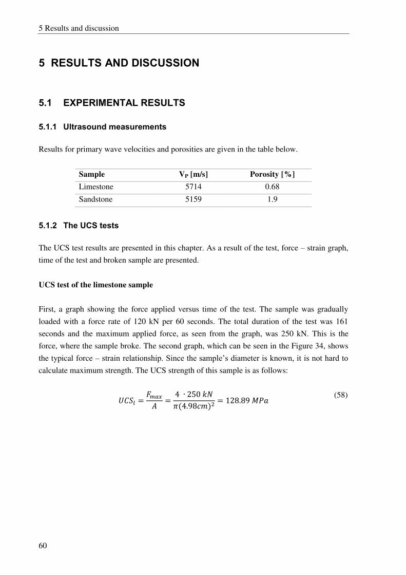
5 Results and discussion
60
5 RESULTS AND DISCUSSION
5.1 EXPERIMENTAL RESULTS
5.1.1 Ultrasound measurements
Results for primary wave velocities and porosities are given in the table below.
Sample VP [m/s] Porosity [%]
Limestone 5714 0.68
Sandstone 5159 1.9
5.1.2 The UCS tests
The UCS test results are presented in this chapter. As a result of the test, force – strain graph,
time of the test and broken sample are presented.
UCS test of the limestone sample
First, a graph showing the force applied versus time of the test. The sample was gradually
loaded with a force rate of 120 kN per 60 seconds. The total duration of the test was 161
seconds and the maximum applied force, as seen from the graph, was 250 kN. This is the
force, where the sample broke. The second graph, which can be seen in the Figure 34, shows
the typical force – strain relationship. Since the sample’s diameter is known, it is not hard to calculate maximum strength. The UCS strength of this sample is as follows:
(58)
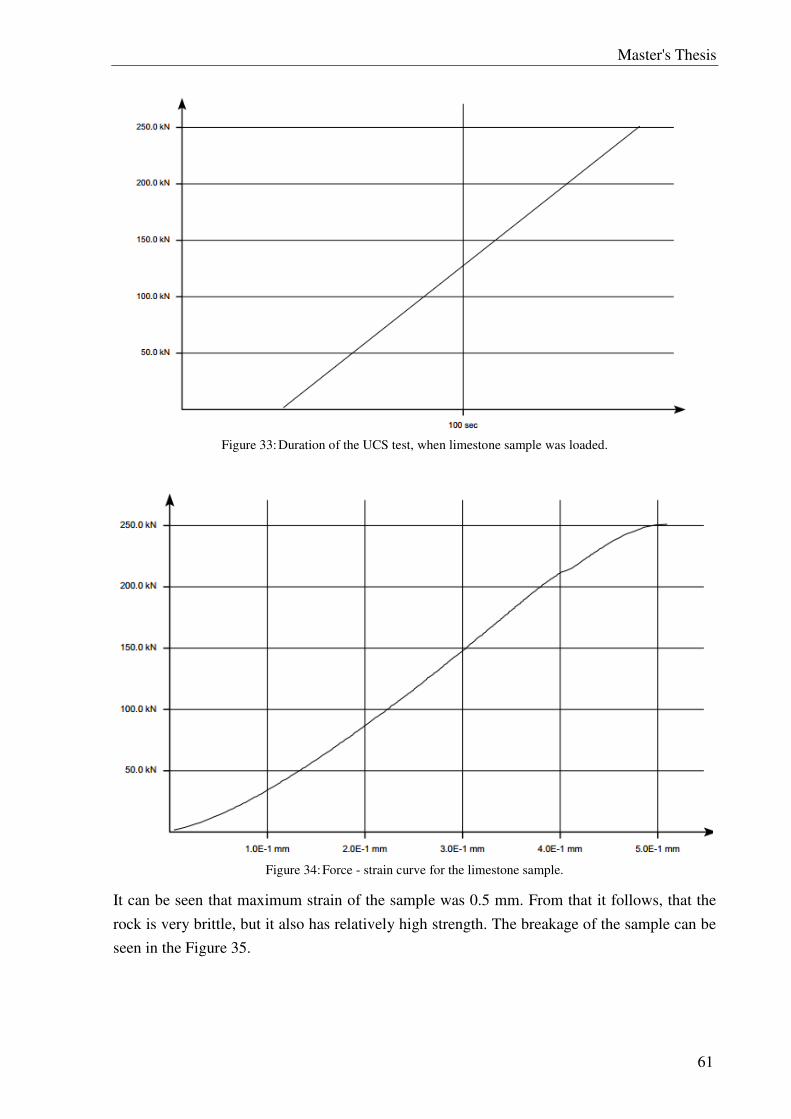
Master's Thesis
61
Figure 33: Duration of the UCS test, when limestone sample was loaded.
Figure 34: Force - strain curve for the limestone sample.
It can be seen that maximum strain of the sample was 0.5 mm. From that it follows, that the
rock is very brittle, but it also has relatively high strength. The breakage of the sample can be
seen in the Figure 35.
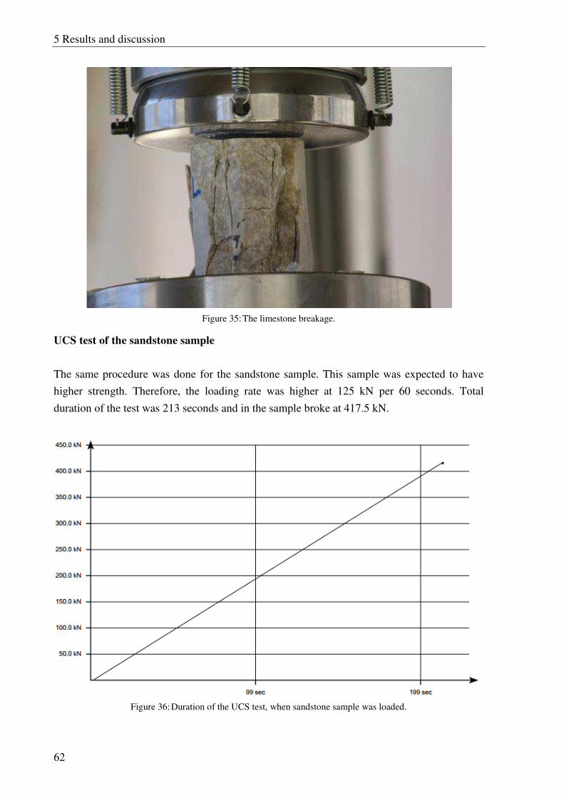
5 Results and discussion
62
Figure 35: The limestone breakage.
UCS test of the sandstone sample
The same procedure was done for the sandstone sample. This sample was expected to have
higher strength. Therefore, the loading rate was higher at 125 kN per 60 seconds. Total
duration of the test was 213 seconds and in the sample broke at 417.5 kN.
Figure 36: Duration of the UCS test, when sandstone sample was loaded.
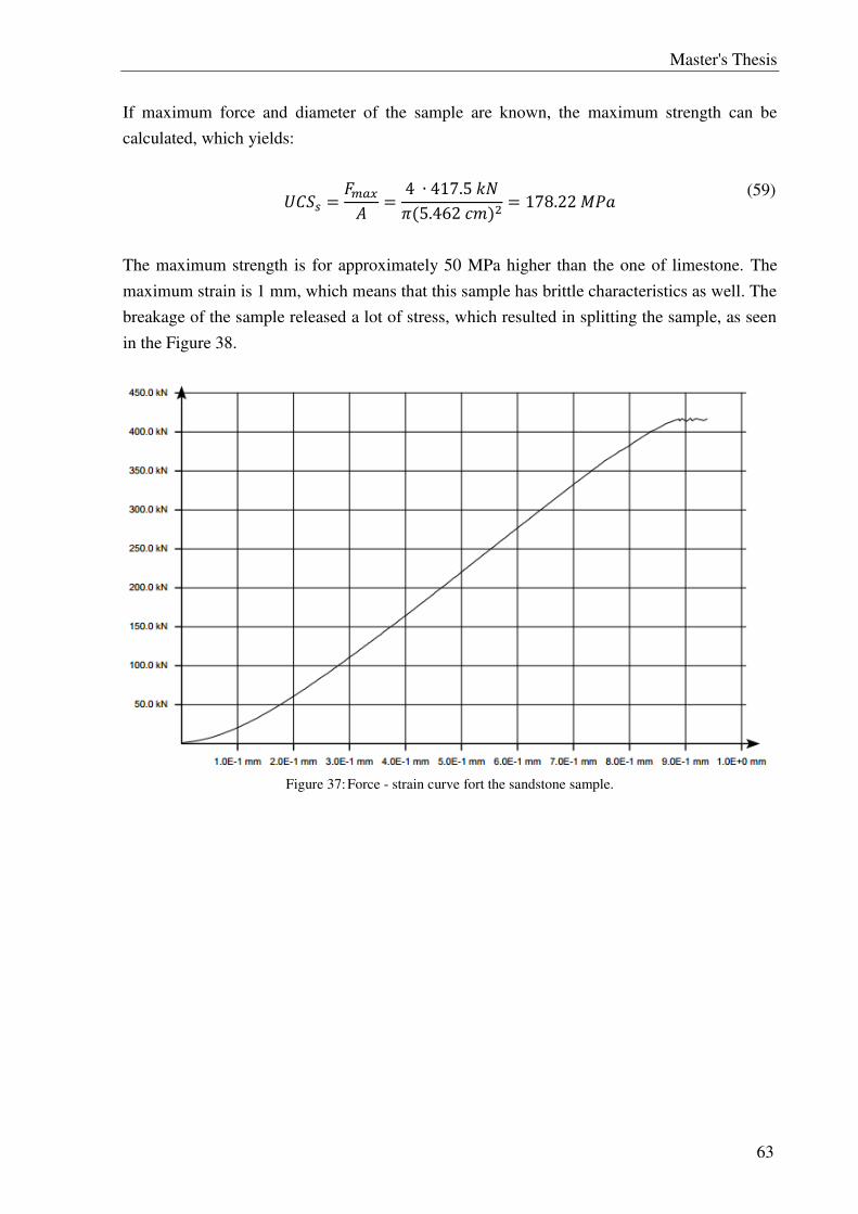
Master's Thesis
63
If maximum force and diameter of the sample are known, the maximum strength can be
calculated, which yields:
(59)
The maximum strength is for approximately 50 MPa higher than the one of limestone. The
maximum strain is 1 mm, which means that this sample has brittle characteristics as well. The
breakage of the sample released a lot of stress, which resulted in splitting the sample, as seen
in the Figure 38.
Figure 37: Force - strain curve fort the sandstone sample.
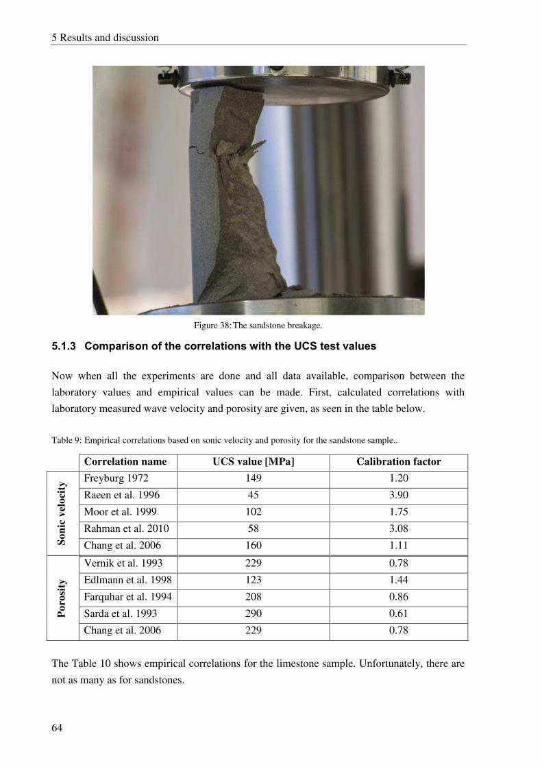
5 Results and discussion
64
Figure 38: The sandstone breakage.
5.1.3 Comparison of the correlations with the UCS test values
Now when all the experiments are done and all data available, comparison between the
laboratory values and empirical values can be made. First, calculated correlations with
laboratory measured wave velocity and porosity are given, as seen in the table below.
Table 9: Empirical correlations based on sonic velocity and porosity for the sandstone sample..
Correlation name UCS value [MPa] Calibration factor
Son
ic v
elocit
y Freyburg 1972 149 1.20
Raeen et al. 1996 45 3.90
Moor et al. 1999 102 1.75
Rahman et al. 2010 58 3.08
Chang et al. 2006 160 1.11
Poro
sity
Vernik et al. 1993 229 0.78
Edlmann et al. 1998 123 1.44
Farquhar et al. 1994 208 0.86
Sarda et al. 1993 290 0.61
Chang et al. 2006 229 0.78
The Table 10 shows empirical correlations for the limestone sample. Unfortunately, there are
not as many as for sandstones.
Master's Thesis
65
Table 10: Empirical correlations based on sonic velocity and porosity for the limestone sample.
Correlation name UCS value [MPa] Calibration factor
Son
ic
vel
ocit
y Chang et al. 2006 135 0.95
Golubev 1973 200 0.61
Militzer 1973 58 2.20
Porosity Farquhar et al.
1994 174 0.74
After the results above, it can be seen that calibration factors vary significantly. Therefore, the
correlations should be used with care and according to the procedure, which is described in
the next chapter. Raeen et al. 1996, Rahman et al. 2010 and Militzer 1973 correlations are not
recommended for use in this case. They were used to show how big the differences can be.
However, Chang et al. 2006 correlations prove to be the best ones and need calibration factors
of 1.11 and 0.95 for sandstone and limestone, respectively. This proves that high number of
tests on different samples yield the best result. Moreover, it can be seen that porosity
correlations usually overestimate the real value, whereas sonic velocity correlations
underestimate the real value.
5.1.4 Process of obtaining rock properties from logs
After the experiments, extensive literature review and comparison were made, a flow chart
showing the process can be given. The flow chart is shown in the figure below. Two flow
charts were made; one for a new field, where number of coring samples are limited and the
second one for a new field, where numerous coring samples are available. The differences
between the two will be expressed in the next paragraphs.
Figure 39 shows the second example, where numerous coring samples are available. Like in
any operation, drilling to the section of interest is the first step. Second, coring of the
formation should take place and, ideally, several samples within one formation are taken. The
best diameter size would be around two inches with a four inches length. If ten samples are
taken, the core should be around 40 inches long (around 3.5 feet), which usually should not be
a problem. Next, if LWD is used then log data are already available and conventional logging
is not needed. If no, then logging to the end of formation is conducted. The most important
logs (rock properties wise) are sonic, density and gamma ray. After porosity values, travel
times or gamma ray radiation are measured, values, marked as y in the figure, are derived. It
is important to correlate these values with coring depth and correct them if necessary.
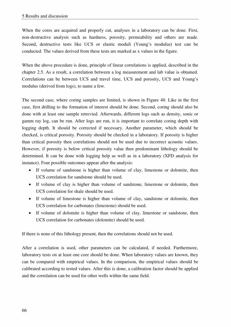
5 Results and discussion
66
When the cores are acquired and properly cut, analyses in a laboratory can be done. First,
non-destructive analysis such as hardness, porosity, permeability and others are made.
Second, destructive tests like UCS or elastic moduli (Young’s modulus) test can be conducted. The values derived from these tests are marked as x values in the figure.
When the above procedure is done, principle of linear correlations is applied, described in the
chapter 2.5. As a result, a correlation between a log measurement and lab value is obtained.
Correlations can be between UCS and travel time, UCS and porosity, UCS and Young’s modulus (derived from logs), to name a few.
The second case, where coring samples are limited, is shown in Figure 40. Like in the first
case, first drilling to the formation of interest should be done. Second, coring should also be
done with at least one sample retrevied. Afterwards, different logs such as density, sonic or
gamm ray log, can be run. After logs are run, it is important to correlate coring depth with
logging depth. It should be corrected if necessary. Another parameter, which should be
checked, is critical porosity. Porosity should be checked in a laboratory. If porosity is higher
than critical porosity then correlations should not be used due to incorrect acoustic values.
However, if porosity is below critical porosity value then predominant lithology should be
determined. It can be done with logging help as well as in a laboratory (XFD analysis for
instance). Four possible outcomes appear after the analysis:
If volume of sandstone is higher than volume of clay, limestone or dolomite, then
UCS correlation for sandstone should be used.
If volume of clay is higher than volume of sandstone, limestone or dolomite, then
UCS correlation for shale should be used.
If volume of limestone is higher than volume of clay, sandstone or dolomite, then
UCS correlation for carbonates (limestone) should be used.
If volume of dolomite is higher than volume of clay, limestone or sandstone, then
UCS correlation for carbonates (dolomite) should be used.
If there is none of this lithology present, then the correlations should not be used.
After a correlation is used, other parameters can be calculated, if needed. Furthermore,
laboratory tests on at least one core should be done. When laboratory values are known, they
can be compared with empirical values. In the comparison, the empirical values should be
calibrated according to tested values. After this is done, a calibration factor should be applied
and the correlation can be used for other wells within the same field.
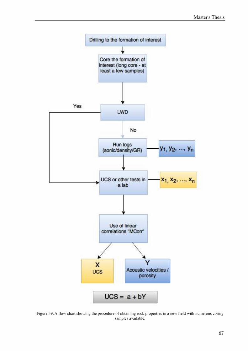
Master's Thesis
67
Figure 39: A flow chart showing the procedure of obtaining rock properties in a new field with numerous coring
samples available.
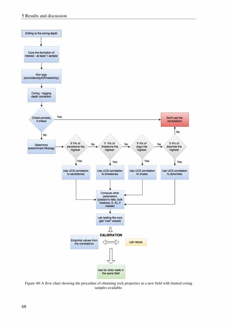
5 Results and discussion
68
Figure 40: A flow chart showing the procedure of obtaining rock properties in a new field with limited coring
samples available.
Master's Thesis
69
5.1.5 Advantages and Disadvantages of Obtaining Rock Properties from Logs
There are numerous advantages using the method described in the previous chapters. Some of
them are:
It is very cost effective; it can save up to 70 % of resources compared to conventional
coring and laboratory testing. UCS and laboratory tests which obtain rock properties
are usually costly and time consuming. A problem is that such laboratory is usually
not in field. Therefore, samples are transported to the location, which makes the
process even more time consuming.
If LWD is used, this method can provide real-time information about rocks. This
makes it very attractive for all other analysis such as drilling dynamics.
A continuous profile can be made with this method. It means that there is more
information about longer sections, than just those which are cored.
It can be used in wells, which are not planned to be cored. Additional information is
therefore available.
The method can be used in field.
However, the method is far from perfect and therefore has several disadvantages such as:
The accuracy of the empirical values can be questionable due to changing formation
composition.
Sonic and density log are not always used. Therefore, this method cannot be used,
except if additional correlations are used to correlate other logs with sonic or density
log.
It does not work for very loose or unconsolidated formations.
It needs to be calibrated when used in a new field. The problem could be solved with
an extra big database of correlated values. However, such database is not available to
date.
Due to low depth investigation of logging tools, the data might not be “real”, especially if mud invaded the near wellbore during drilling operation.
5.2 RECOMMENDED PRACTICES TO AVOID DRILLING
DYNAMICS DYSFUNCTIONS
After extensive literature review and analysis of case studies, the best practices to mitigate or
avoid drilling dynamics dysfunctions can be given. The recommendations will be given for
the most often phenomena which can be encountered during drilling operations. For each
phenomenon optimization of surface parameters will be described, potential for damage
evaluated and BHA design changes recommended.
5 Results and discussion
70
5.2.1 Full Stick Slip (FSS)
As described in previous chapters, full stick slip phenomenon can cause a potential damage.
On the scale from low to high, the damage can be evaluated as moderate. Nevertheless, it can
significantly increase NPT and it can decrease well path accuracy. To mitigate this effect with
surface parameters, weight on bit should be reduced and the revolutions increased.
Additionally, there are more options if a BHA component or well plan can be changed:
Friction can be reduced: use of rolling elements, mechanical reduction friction subs,
rolling reamers, mud lubrication (use of oil based mud).
Reduce bit aggressiveness: a short gauge bit is more aggressive and a long gauge bit
tends to be less aggressive and create a smoother hole.
Torque control devices or torque mitigation devices; such as soft torque – the most
often used tool for stick slip mitigation. The soft torque is based on an algorithm
which counteracts drill string fluctuation. It calculates set parameters for the drive
controller.
5.2.2 Low Frequency Torsional Oscillation (LFTO)
Low frequency torsional oscillation is common and as the name suggest they occur at low
frequencies which usually do no exceed 100 Hz. Because of low frequencies this effect cannot
be mitigated with surface parameters optimization. Additionally, the damage which this
oscillation can cause is rather low. A major issue could be that this oscillations lead to fatigue
which is very hard to detect. Moreover, increase in torsional rigidity of the BHA or the
drillstring would lower the occurrence of this phenomenon. Like in the previous case, torque
based surface drive control can slightly reduce the dysfunctions.
5.2.3 High Frequency Torsional Oscillation (HFTO)
On the contrary to LFTO, high frequency torsional oscillation occurs at high frequencies, well
above 200 Hz. Previously, it was believed that such oscillation does not exist which led to
many unexplained failures. Damage potential for this phenomenon is high. The only surface
parameter which can be optimized to reduce the damage is to reduce WOB. Additionally,
BHA redesign, bit aggressiveness and torque control should be discussed.
5.2.4 Random Torsional Vibration
A vibration which occurs without any particular pattern or does not follow the phenomena
previously described is called a random torsional vibration. This effect can potentially cause

Master's Thesis
71
damage, which is usually neither particularly low nor high. It can be classified as medium
damage potential. Reducing WOB and increasing RPM would both mitigate the occurrence of
this effect.
5.2.5 BHA Whirl
BHA whirl can further lead to other effects, therefore it is important to reduce it in the first
place. Similarly, it can be reduced with reduced WOB. A more effective solution would be
the BHA redesign which would include friction reducing tools such as rolling reamers and
anti-whirl bits. Additionally, use of lubrication is recommended such as oil based mud for
instance.
6 Conclusion
72
6 CONCLUSION
Comparison of empirical correlations which use sonic velocity and porosity as input
parameters to derive uniaxial compressive strength was among other objectives of this thesis.
Other objectives include verification of the correlations with an experiment, recommended
procedure to use empirical correlations in field and investigation of how rock properties
(including formation dip, friction factor and rock strength) affect drilling dynamics behaviour.
The work which was done in this thesis includes an experiment in which sandstone and
limestone samples were acquired and UCS, sonic velocity and porosity values were measured.
These values were correlated with use of correlations from Farquhar et al. (1994), Militzer
(1973), Golubev (1973), Freyburg (1972), Vernik et al. (1993), Sarda et al. (1993), Raeen et
al. (1996), Moor et al. (1999), Rahman et al. (2010), and Chang et al. (2006). As a result, a
flow chart showing the recommended procedure to use these correlations was made.
Additionally, importance of knowing the rocks strength in regard to drilling dynamics was
researched.
The scope of this thesis did not include an experiment in which relationship between friction
factor and drilling dynamics would be empirically analysed. However, this is a good topic for
further research.
The following conclusions can be made:
The correlations from Freyburg (1972), Vernik et al. (1993) , Farquhar et al. (1994)
and Chang et al. (2006) showed the best results.
The correlations above showed good results, whereas many others like Raeen et al.
(1996), Rahman et al. (2010) and Moor et al. (1999) needed calibration factor higher
than two which is not acceptable. Many of them work only for certain types of rocks
and for certain fields. Therefore, they are very location sensitive.
Correlations which use porosity as a parameter to derive UCS usually overestimate the
real value, whereas the ones which use sonic velocity underestimate them.
Empirical correlations are limited in use and can only be used for sandstone, shale,
dolomite or limestone dominated lithology.
If the correlation between sonic velocity or porosity and UCS wants to be determined
in a field, where numerous coring samples are available, then linear correlations
principle should be used, as described in chapter 2.5.
If the empirical correlations are used in a field, where coring samples are limited, but
there is at least one available, then the dominant lithology correlation should be used
Master's Thesis
73
and properly correlated with the test value, as described in chapter 5.1.4. Afterwards,
the calibration factor should be applied to the empirical values of new wells (within
the same field).
In the future, more cores should be tested. As a result, a bigger worldwide database of
correlations would be available. This proved to be true, since the correlation (of Chang
et al. 2006) had the largest number of tests on different samples and yielded the best
result. However, the problem is that the industry is usually very sensitive when it
comes to data sharing.
Drilling dynamics can be studied after BHA design, drillstring configuration, mud properties,
operational parameters, hydraulics and rock properties are known. It was found out that rock
properties greatly affect drilling dynamics phenomena as well as BHA design. After the
analyses the following conclusions can be made:
Drilling dynamics is a complex topic, which is relatively unknown and undiscovered.
Therefore, more research is needed in the future.
There are four most common phenomena that occur due to vibration: FSS, LFTO,
HFTO, random torsional oscillation and BHA whirl.
A special care about drilling dynamics dysfunctions should be taken because they can
increase costs, NPT, tool failures rate and possibility of missing the target.
The most destructive dysfunctions appear in wellbores with diameter bigger than 12
inches. Transition from soft to hard and abrasive formation is also a perfect
environment for higher oscillations. Vibrations reach critical level much higher if
there is calcite or sandstone (high UCS rocks) stringer in a soft formation as described
in chapter 3.2.7.
Appropriate measurement system is necessary to detect vibrations. Advanced
accelerometers should be used to record frequencies above 200 Hz. After data are
obtained, analysis should be done and improvement made, such as BHA redesign, use
of lubrication, roller reamers or soft torque system. Additionally, surface parameters
could be optimized in order to mitigate the effect.
Vibrations which occur at higher frequencies are proved to be as hazardous as the
ones, which occur at lower frequencies.
7 References
74
7 REFERENCES
Wyllie, M.R.J., Gregory, A.R. and Gardner, L.W. Elastic Wave Velocities in Heterogeneous
and Porous Media. Geophysics, 21, 1956, pp 41-70
Raaen, M.A. and Hovem, A.K. 1996. FORMEL: A Step Forward in Strength Logging.
Colorado, USA.
Borba,. M. A., Ferreira, H. F., Santos, R. S. E. et al. 2014. UCS Estimation through Uniaxial
Compressive Test, Scratch Test and Based Log Empirical Correlation. Goiania, Brazil.
York, P., Pritchard, D., Dodson, K. J. and Dodson, T. 2009. Eliminating Non-Productive
Time Associated With Drilling Trouble Zones. Texas, USA.
Han, D., Batzle, M. and Liu, J. 2006. Acoustic Property of Heavy Oil – Measured Data.
Annual Meeting, New Orleans.
Wang, Z., Nur, A.M., and Batzle, M.L. 1990. Acoustic Velocities in Petroleum Oils. J Pet
technology 42 (2): 192-200. SPE-18163-PA.
Hashin, Z., and Shtrikman, S. 1963. A variational approach to the theory of the elastic
behaviour of multiphase materials. J. Mech. Phys. Solids 11.
Edlmann, K., Somerville, J.M., Smart, B.G.D., Hamiltono, S.A., Crawford, B.R. 1998.
Predicting Rock Mechanical Properties from Wireline Porosities. Trondheim, Norway. SPE
47344
Farquhar, R.A., Somerville, J.M., and Smart, B.G.D. 1994. Porosity as a Geomechanical
Indicator: An Application of Core and Log Data and Rock Mechanics. London, UK. SPE
28853
Odunlami, T., Soroush, H., Kalathingal, P., and Somerville, J. 2011. Log-Based Rock
Property Evaluation - A New Capability in a Specialized Log Data Management Platform.
SPE. doi:10.2118/149050-MS
Sarda, J.P., Wicquart. E., Hannaford. K., and Deflander, J.P. 1993 Use of Porosity as a
Strength Indicator for Sand Production Evaluation. Houston, Texas, 3-6 October. SPE 26454
Master's Thesis
75
Moos, D., Zoback, D.M., and Bailey, L. 1999. Feasibility Study of the Stability of Openhole
Multilaterals. Cook Inlet, Alaska. Oklahoma, USA.
Rahman, K., Khaskar, A., and Kayes, T. 2010. An Integrated Geomechanical and Passive
Sand-Control Approach to Minimizing Sanding Risk From Openhole and Case-and-
Perforated Wells. Denver, USA.
Weingarten, J.S., and Perkins, T.K. 1995. Prediction of Sand Production in Gas Wells:
Methods and Gulf of Mexico Case Studies.
Horsrud, P. 2001. Estimating Mechanical Properties of Shale From Empirical Correlations.
SPE Drilling & Completion, June. SPE 56017
Buorgoyne, A.T., Millheim, K.K., Chenevert, E.M., and Young, F.S. 1986. Applied Drilling
Engineering. USA. ISBN 1-55563-001-4
Carmichael, S.R. 1990. Practical Handbook of Physical Properties of Rocks and Minerals.
Florida, USA. ISBN 0-8493-3703-8
Fjaer, E., Holt, M.R., Horsrud, P., Raaen, M.A., and Risnes, R. 2008. Petroleum Related Rock
Mechanics, 2nd
Edition. ISBN 978-0-444-50260
Mavko, G., Mukerji, R., and Dvorkin, J. 1998. The Rock Physics Handbook: Tools for
Seismic Analysis in Porous Media. ISBN 0- 521-62068-6
Allen, B.M. 1987. BHA Lateral Vibrations: Case Studies and Evaluation of Important
Parameters. New Orleans, USA. SPE/IADC 16110
Bailey, R.J. and Remmert, M.S. 2009. Managing Drilling Vibrations Through BHA Design
Optimization. Doha, Qatar. IPTC 13349
Burgess, M.T., McDaniel, L.G., and Das, K.P. 1987. Improving BHA Tool Reliability With
Drillstring Vibration Models: Field Experince and Limitations. New Orleans, USA. SPE
16109
Ramizer, S. and Aguilar, R. 2010. Evolution of Rotary Steerable BHA Designs in Mexico
Offshore: Solution to Stop Multiple Drillstring Failures in High-Vibration Environment.
Lima, Peru. SPE 138963
7 References
76
Chatar, C. and Blyth, M. 2011. Effective BHA Design and Vibration Modeling for Improving
the Quality of Sonic Measurements. Amsterdam, the Netherlands. SPE/IADC 140326
Chen, K.C.D. 2007. Integrated BHA Modeling Delivers Optimal BHA Design. Cairo, Egypt.
SPE/IADC 106935
Mason, S.J. and Sprawls, M.B. 1998. Addressing BHA Whirl: The Culprit in Mobile Bay.
New Orleans, USA. SPE 52887
Payne, M.L. 1992. Drilling Bottom-Hole Assembly Dynamics. PhD Thesis. Texas, USA.
Nicholson, W.J. 1994. An Integrated Approach to Drilling Dynamics Planning, Identification,
and Control. Dallas, USA.
Reckmann, H., Jogi, P., Kpetehoto, F., Chandrasekaran, S., and Macpherson, J. 2010. MWD
Failure Rates Due to Driling Dynamics. New Orleans, USA. IADC/SPE 127413
Oueslati, H., Jain, R.J., Ledgerwood, L.W., and Pessier, R. 2013. New Insights Into Drilling
Dynamics Through Hihg-Frequency Vibration Measurement and Modeling. New Orleans,
USA. SPE 166212
Lake, W.L. 2007. Petroleum Engineering Handbook, Volume II. SPE. ISBN:978-1-55563-
126-0
JPT staff, _. 1999. Downhole Dynamics Data Increases Drilling-Process Control. SPE.
doi:10.2118/0299-0038-JPT
Lines, L. A., Mauldin, C. L., Hill, J. W., & Aiello, R. A. 2014. Advanced Drilling Dynamics
Sensor Allows Real-Time Drilling Optimization, Damage Prevention and Condition
Monitoring of RSS and LWD BHAs. SPE. doi:10.2118/170586-MS
Elsborg, C. C., & Grindhaug, G. 2006. Planning and Detailed BHA Vibration Modeling Lead
to Performance Step Change Drilling Deviated 24-in. Hole Section, Offshore Norway. SPE.
doi:10.2118/99126-MS
Fichter, L.S. 2000. A Basic Sedimentary Rock Classification. James Madison University,
Virginia, USA.
Master's Thesis
77
Boggs, J.R. 2000. Principles of sedimentology and stratigraphy, 3rd
edition. Toronto, Canada.
ISBN 0-13-099696-3
Hood, J., Hovden, J., Heisig, G., Ernesti, K. D., and Knipper, A. 2003. Real-Time BHA
Bending Information Reduces Risk when Drilling Hard Interbedded Formations. SPE.
doi:10.2118/79918-MS
Bardet, J.P. 1997. Principles of Unconfined Compression Test. Prentice-Hall, New Yersey,
USA.
Oueslati, H., Hohl, A., Makkar, N., Schwefe, T., & Herbig, C. 2014. The Need for High
Frequency Vibration Measurement Along With Dynamics Modeling to Understand the
Genesis of PDC Bit Damage. SPE. doi:10.2118/167993-MS
Jain, J. R., Oueslati, H., Hohl, A., Reckmann, H., Ledgerwood III, L. W., Tergeist, M., … Ostermeyer, G. P. 2014. High-Frequency Torsional Dynamics of Drilling Systems: An
Analysis of the Bit-System Interaction. SPE. doi:10.2118/167968-MS
Pastusek, P. E., Sullivan, E., & Harris, T. M. 2007. Development and Utilization of a Bit
Based Data Acquisition System in Hard Rock PDC Applications. SPE. doi:10.2118/105017-
MS
Gegenhuber, N. 2016. Interpretation of Elastic Properties for Magmatic and Metamorphic
Rock Types. International Journal of Rock Mechanics & Mining Sciences 88.
http://dx.doi.org/10.1016/j.ijrmms.2016.07.007
Gegenhuber, N., Pupos, J. 2015. Rock Physics Template from Laboratory Data for
Carbonates. Journal of Applied Geophysics 114.
http://dx.doi.org/10.1016/j.jappgeo.2015.01.005
Pettijohn, F.J. 1983. Sedimentary Rocks. Harpercollins, 3rd
Ed.
Moore, C. H., Wade, J. W. 2013. Carbonate Reservoirs. Elsevier, 2nd
Ed.
Ahr, M. W., 2008. Geology of carbonate Reservoirs: The Identification, Description, and
Characterization of Hydrocarbon Reservoirs in Carbonate Rocks. John Wiley and Sons. DOI:
10.1002/9780470370650
7 References
78
Ehrenberg, S. N., & Nadeau, P. H. 2005. Sandstone vs. Carbonate petroleum reservoirs: A
global perspective on porosity-depth and porosity-permeability Relationships. The AAPG
Journal.
Mwanga, A., Rosenkranz, J., and Lamberg P. Testing of Ore Comminution Behaviour in the
Geometallurgical Context – A Review. Minerals, 276-297. DOI: 10.3390/min5020276
Inglis, T.A. Petroleum engineering and development studies. Vol. 2: Directional drilling.
USA. DOI: 10.1007/978-94-017-1270-5
Mihailović, K. 2002. Regresiona Analiza: objektivni pristup određivanja parametara funkcija. University of Belgrade, Belgrade.
Mitchell, R. F., & Samuel, G. R. (2007). How Good is the Torque-Drag Model? SPE.
doi:10.2118/105068-MS
Mirhaj, A., Kaarstad, E., and Aadnoy, B. S. (2010). Minimizing Friction In Shallow
Horizontal Wells. SPE. doi:10.2118/135812-MS
Gee, R., Hanley, C., Hussain, R., Canuel, L., and Martinez, J. (2015). Axial Oscillation Tools
vs. SPE. doi:10.2118/173024-MS
Quigley, M. S., Dzialowski, A. K., and Zamora, M. (1990). A Full-Scale Wellbore Friction
Simulator. SPE. doi:10.2118/19958-MS