Venture Capital Contracts and Market Structure∗

Roman Inderst† Holger M. Müller‡

First Draft: February 2000. This Draft: January 2002

∗We are indebted to Per Strömberg for valuable comments and suggestions. Thanks also to Patrick Bolton,

Mike Burkart, Paul Gompers, Denis Gromb, Thomas Hellmann, Martin Hellwig, Josh Lerner, Kjell Nyborg, Enrico

Perotti, Elu von Thadden, Masako Ueda, Andy Winton, Julie Wulf, and seminar participants at Amsterdam,

Humboldt, Mannheim, Stockholm School of Economics, Tilburg, the Columbia-NYU-Princeton-Wharton-Yale

Five Star Conference on Research in Finance at NYU (2001), the workshop “Strategic Interactions in Relationship

Finance: Bank Lending and Venture Capital” at LSE (2001), the workshop “Finance for the XXI Century” in

Amsterdam (2001), and the European Summer Symposium in Financial Markets (ESSFM) in Gerzensee (2001)

for helpful comments. Earlier versions of this paper circulated under the titles “Competition and Efficiency in

the Market for Venture Capital” and “Market Structure, Contracting, and Value Creation in Venture Capital

Finance.”

†London School of Economics, FMG, & CEPR. Address: Department of Economics & Department of Account-

ing and Finance, London School of Economics, Houghton Street, London WC2A 2AE. Email: r.inderst@lse.ac.uk.

‡New York University & CEPR. Address: Department of Finance, Stern School of Business, New York Uni-

versity, 44 West Fourth Street, Suite 9-190, New York, NY 10012-1126. Email: hmueller@stern.nyu.edu

1

Abstract

We examine the relation between optimal venture capital contracts and the supply and

demand for venture capital. Both the composition and type of financial claims held by the

venture capitalist and entrepreneur depend on the market structure. Beside, different market

structures involve different optimal forms of transferring utility: sometimes it is optimal to

transfer utility via equity stakes, sometimes it is optimal to use debt. Transferring utility via

equity stakes affects incentives. Consequently, the net value created, the success probability, the

market value, and the performance of venture-capital backed investments depend on the supply

and demand for capital. Similarly, venture capitalists face different incentives to screen projects

if the capital supply is low or high. We then endogenize the capital supply and study the relation

between venture capital contracts and entry costs, public policy, investment profitability, and

market transparency. Finally, we show that entry by inexperienced investors creates a negative

externality for the value creation in ventures financed by (regular) venture capitalists.

2

1 Introduction

Do optimal financial contracts depend on the supply and demand for capital? And if so, how?

In this paper, we address this question in the context of venture capital contracting. We exam-

ine whether, and how, optimal venture capital contracts vary with the supply and demand for

capital, or more generally, the level of competition in the venture capital market. Pursuing this

question within the traditional financial contracting framework is problematic, as it assumes

that one side (typically the entrepreneur) has all the market power. We hence depart from the

traditional paradigm and embed venture capital contracting in a search market where entrepre-

neurs and venture capitalists bargain over optimal contracts. Both the supply and demand for

capital are competitive in the sense that there are many venture capitalists and many entrepre-

neurs. The market power of each side is determined by the ratio of supply to demand. A high

ratio implies that the degree of competition among venture capitalists is high.

We find that both the composition and type of financial claims held by the venture capitalist

and entrepreneur depend on the market structure, or degree of competition. If the degree

of competition is either low or high, one side holds a mix of debt and equity and the other

side holds straight equity. If the degree of competition is intermediate, both sides hold debt

and equity. Generally, a change in the ratio of supply to demand affects market powers and

therefore the distribution of surplus. The question is whether utility should be transferred via

equity or debt. As a guiding principle, utility should be transferred at least cost, i.e., in a way

that minimizes incentive distortions. We show that different competition levels entail different

optimal forms of transferring utility. If the level of competition is either low or high, utility is

transferred by changing the equity component of the optimal contract. If the level of competition

is intermediate, utility is transferred by changing the debt component.

Work by Lerner (1995), Hellmann and Puri (2001), and Kaplan and Strömberg (2001b)

indicates that venture capital contracting may be appropriately viewed as a double-sided moral-

hazard problem.1 Venture capitalists monitor the progress of the firm, give advice, provide

entrepreneurs with access to consultants, investment bankers, and lawyers, negotiate with sup-

pliers, and play an active role in the building up of human resources and recruiting of senior

management. Under double-sided moral hazard, the second-best solution requires that both

the venture capitalist and the entrepreneur hold sufficiently large equity stakes. Actual equity

stakes, however, are determined by bargaining, where outside options depend on the level of

competition in the capital market. For low and high levels of competition, outside options are

strongly asymmetric, which implies that equity stakes , and hence incentives, deviate from the

1Theoretical papers modelling venture capital contracting as a double-sided moral-hazard problem include

Casamatta (2000), Cestone (2001), Renucci (2000), Repullo and Suarez (2000), and Schmidt (2000).

3

second-best optimum. (While riskless debt can be used to transfer utility without affecting

incentives, the total amount of riskless debt available is limited.)

This has the following additional implications: the net value created in ventures is a hump-

shaped function of the degree of competition. If efforts are substitutes, the success probability,

the market value, and the average performance of venture-capital backed investments are in-

creasing in the degree of competition if the entrepreneur’s contribution is more important, and

decreasing if the venture capitalist’s contribution is more important. If efforts are complements,

the success probability, market value, and average performance are all hump-shaped functions

of the degree of competition. Most of our results remain yet to be tested. The ones that have

been tested, however, are consistent with the empirical evidence. We provide a discussion of the

empirical evidence at the end of this paper.

In an extension of the model, we consider projects (or entrepreneurs) of low and high quality.

Prior to making his investment, the venture capitalist can screen the project. We show that

venture capitalists screen more if the degree of competition is low, and less if the degree of

competition is high.

A caveat is in order here. The above implications are based on the notion that financial

claims have a first-order effect on incentives. While it is difficult to say what motivates venture

capitalists in practice, the following quote suggests that financial claims matter.2

In an investment memo regarding a company in the financial information industry,

a venture capitalist outlines a number of actions that he will undertake to assist

the company. Among the risk factors which the venture capitalist worries about is

whether he “can [...] get enough money at work, or ownership in the company, to

warrant allocating these extra resources.”

Similarly, Kaplan and Strömberg (2001b) conclude that equity incentives increase the likelihood

that venture capitalists perform value-added support activities.

In the second part of the paper, we take the argument one step further and examine factors

that potentially affect the capital supply. We consider entry costs, public policy, investment

profitability, and market transparency. To investigate the role of these factors, we endogenize

the entry decision of venture capitalists, thereby endogenizing the degree of competition in the

capital market. An individual venture capitalist entering the market does not take into account

the effect of his entry on the overall level of competition, and thus on the bargaining, contracting,

and value creation in other ventures. Depending on the level of competition prevailing in the

market, entry by an individual venture capitalist thus either creates a positive or negative

contracting externality.

2We thank Per Strömberg for this quote.

4

It is frequently argued that the short-run supply of informed capital is fixed, for it takes time

to develop the skills and experience which are necessary to be a good advisor (Gompers and

Lerner 1999). In an extension of the model, we assume that informed capital is in short supply.

There is, however, an abundant potential supply of portfolio investors, i.e., investors who have

capital but no expertise.3 We show that if the level of competition is strong, portfolio investors

not only fail to add value in their own ventures, but also create a negative externality for the

value added in ventures financed by (regular) venture capitalists.

We believe our model of bargaining and search captures important features of real-world

venture capital contracting environments. In our model, deals are struck through bilateral nego-

tiations, and not through auctions or a Walrasian tâtonnement mechanism. Both entrepreneurs

and venture capitalists must actively look for deals. They can quit negotiations at any time and

team up with somebody else. Finding a suitable partner takes time, however, and is easier the

greater the supply of potential partners relative to the demand. Everyone is aware of his own

and his partner’s outside options, and this affects the outcome of the negotiations.4 Finally,

search models have appealing economic properties. For instance, in our model outside options,

and hence contracts, adjust gradually to changes in the degree of competition. By contrast, in

a Walrasian market the outcome is a bang-bang solution where the shorter side of the market

has the entire market power. This can have extreme implications: if there are K venture capi-

talists and K− 1 entrepreneurs, entrepreneurs have the entire market power. If there are K +1entrepreneurs, however, venture capitalists have the entire market power.

By embedding venture capital contracting in a market environment, our paper goes beyond

papers studying venture capital contracting in isolation. On the other hand, unlike many of

these papers, our simple model falls short of explaining the richness of cash flow and control

rights found in real-world venture capital contracts Michelacci and Suarez (2000) also have

a search-based model of start-up financing. Unlike our model, Michelacci and Suarez do not

consider incentive contracts or contracting inefficiencies. Instead, they consider search inefficien-

cies, using an insight from the search literature that entry creates externalities for the matching

chances of other market participants. In Aghion, Bolton, and Tirole (2000), the limited partners

3There is evidence of inexperienced investors entering the venture capital industry at times when the market is

“hot”. For instance, the Economist notes: “[a] host of new entrants are now dabbling in venture capital, ranging

from ad hoc groups of MBAs to blue-blooded investment banks such as J.P. Morgan, to sports stars and even the

CIA.” Money to Burn, the Economist, May 27, 2000.

4Entrepreneurs typically strike better deals when the supply of capital is abundant. The following is a statement

comparing the boom period of the most recent venture capital cycle with the aftermath: “if you went into a [...]

start-up three to six months ago, you almost certainly got a very bad deal. Companies could ask for anything

they wanted [in terms of valuation]. Now entrepreneurs are much more realistic.” Open Season for Europe’s

Turkeys, Financial Times, January 11, 2001.

5

in a venture partnership (i.e., the investors) must incentivize the venture capitalist to monitor

an entrepreneur. Changes in the market environment that close the gap between the venture

capitalist’s private opportunity cost of capital and the investors’ cost of capital improve the

efficiency of the incentive contract. Inderst (2001) also examines the relationship between com-

petition and contract design. Unlike this paper, he considers screening contracts in an adverse

selection setting. To our knowledge, our paper is the first to investigate the relation between in-

centive contracts and market structure in a moral hazard setting. Finally, we are not the first to

note that constraints on transfer payments may impair contract efficiency. Aghion and Bolton

(1992) and Legros and Newman (2000) both discuss the implications of this for the optimal

allocation of control rights.

2 Non-Technical Overview

Section 3 presents the model. The model consists of three building blocks: i) financial con-

tracting, ii) bargaining, and iii) search. Section 3.1 studies a contracting problem between an

entrepreneur and a venture capitalist. The optimal contract is a combination of equity and risk-

less debt.5 Both the entrepreneur and the venture capitalist can exert effort. Equilibrium effort

levels depend on the way in which the equity is allocated between the two. We first derive the

utility possibility frontier generated by different equity allocations. The undominated segment

of the frontier is called equity frontier. We subsequently add the riskless debt. The idea is to

allocate the debt in a way that minimizes incentive distortions. The utility possibility frontier

generated by different Pareto-optimal contracts is called bargaining frontier. In Section 3.2, the

entrepreneur and venture capitalist bargain over an optimal contract. We apply the generalized

Nash bargaining solution. Reservation values, i.e., outside options, are exogenous. In Section

3.3, we endogenize reservation values by embedding the bargaining problem in a search market

with pairwise matching. Reservation values are determined by the market structure, or degree

of competition, as expressed by the ratio of venture capitalists to entrepreneurs in the market.

The degree of competition is assumed to be exogenous.

Section 4 summarizes the results. Via its effect on reservation values, the degree of compe-

tition determines i) the optimal financial contract, ii) the net value created, i.e., the expected

project return minus aggregate effort costs, iii) the gross surplus, which corresponds to the

market (or IPO) value of the venture if it was sold after effort and investment costs are sunk

but before returns are realized, iv) the expected, or average, performance of the venture-backed

5An alternative interpretation is that the entrepreneur and venture capitalist hold combinations of common

and straight preferred stock, or, with minor qualifications, participating convertible preferred stock. Such claims

are widely used in real-world venture capital contracts (Kaplan and Strömberg 2001a).

6

investment, and v) the success probability of the venture, i.e., the likelihood that the investment

pays off more than it costs. We also study the role of up-front payments.

Section 5 endogenizes the degree of competition by introducing free entry of capital. We

examine the way in which the degree of competition, and thus the optimal contract, net value,

etc., is affected by i) entry costs, ii) regulation and public policy, iii) investment profitability,

and iv) market transparency.

Section 6 considers projects of different quality. We investigate the impact of competition

on the incentives of venture capitalists to screen projects ex ante.

Section 7 introduces a second class of investors: portfolio investors, i.e., investors who have

money but no skills. We examine the effect of entry by portfolio investors on the performance

of investments financed by (regular) venture capitalists.

Section 8 concludes. All proofs are provided in the Appendix.

3 The Basic Model

3.1 Financial Contracting

The Basic Setup

A penniless entrepreneur has a project which requires an investment outlay I > 0. Funding

is provided by a venture capitalist. The project return is Xl ≥ 0 with probability 1 − p andXh > I > Xl with probability p. The success probability p = p (e, a) depends on both the entre-

preneur’s and the venture capitalist’s (unobservable) efforts e ∈ [0, 1] and a ∈ [0, 1], respectively.The corresponding effort cost functions are cE (e) := e2/2αE and cF (a) := a2/2α. All agents

are risk neutral.

The project return can be decomposed into a riskless return equal to Xl and a risky return

paying 0 in the bad state and∆X := Xh−Xl in the good state. With the usual degree of caution,we refer to these as debt and equity. An optimal contract between the entrepreneur and the

venture capitalist specifies i) the venture capitalist’s investment I, ii) the debt 0 ≤ S ≤ Xl held bythe venture capitalist, and iii) the fraction of equity s ∈ [0, 1] held by the venture capitalist.6 InSection 4, we additionally admit up-front payments by the venture capitalist. The entrepreneur

keeps any return not paid to the venture capitalist. The entrepreneur’s utility from the contract

(s, S) is U (s, S) := u (s) +Xl − S, where u (s) := p (1− s)∆X − e2/2αE represents his utility

from the equity allocation s. Likewise, the venture capitalist’s utility from the contract (s, S)

is V (s, S) := v (s) + S − I, where v (s) := ps∆X − a2/2α represents his utility from the equity

allocation s.

6This rules out that one party receives a higher payment in the bad state than in the good state. It is easy to

show that such contracts are never optimal.

7

To simplify the exposition, we proceed in two steps. We first derive the set of Pareto-

optimal u− v combinations. The utility possibility frontier generated by Pareto-optimal equityallocations is called equity frontier. We then add the riskless debt and investment cost and

derive the set of Pareto-optimal U − V combinations. The utility possibility frontier generated

by Pareto-optimal contracts is called bargaining frontier.

The Equity Frontier

The equity frontier u = ψE (v) depicts the utilities u (s) and v (s) for all Pareto-optimal

equity allocations. In general, the precise shape of the equity frontier depends on the production

technology p (e, a) . There are, however, some robust properties that any well-behaved equity

frontier has. These are:

i) the equity frontier is strictly concave,

ii) the sum u (s) + v (s) attains its maximum in the interior of the domain, and

iii) along the equity frontier, v (s) is strictly increasing in s.

The first two properties follow naturally from the fact that the incentive problem is two-sided and

effort costs are strictly convex. Maximizing the sum of utilities then requires balancing the two

incentive problems. Giving one side too big an equity stake is inefficient as it will then produce

at a point where the marginal effort cost is relatively high. Accordingly, the equity allocation

maximizing the total utility lies somewhere in the interior. Denote the point where the total

utility is maximized by (v, u), and the corresponding equity allocation by s. We occasionally

refer to this as the joint-surplus maximizing, or second-best, solution. Clearly, ψ0E (v) = −1.The third property states that the venture capitalist’s utility increases with his equity stake.

Note that this need not be true for dominated segments of the utility possibility frontier, i.e.,

segments that lie not on the equity frontier. (See the following examples.)

We illustrate these properties by means of two examples. The first is based on the linear

technology p (e, a) = da + (1− d) e used in, e.g., Casamatta (2000). The second is based onthe Cobb-Douglas technology p (e, a) = ade1−d used in, e.g., Repullo and Suarez (2000). Under

the linear technology, the two efforts are substitutes while under the Cobb-Douglas technology,

they are complements. While for the remainder of the paper we could work with either of

these technologies (or any other well-behaved technology), we instead use the general notation

u = ψE (v) and assume that properties i)−iii) hold. To make the problem non-trivial, we assumethat the second-best outcome is sufficiently good to allow the venture capitalist to break even,

i.e., that v > I.

Example 1: Linear Technology. To ensure that the equilibrium success probability

has an interior solution, we assume that max {αE (1− d) ,αFd} < 1/∆X . Given some equity

allocation s, the corresponding equilibrium effort choices are a∗(s) = αFds∆X and e∗(s) =

8

αE (1− d) (1− s)∆X , respectively. The equilibrium success probability is

p∗(s) := p(e∗(s), a∗(s)) = ∆XhαFd

2s+ αE (1− d)2 (1− s)i. (1)

The venture capitalist’s and entrepreneur’s utility from the equity allocation s is

v(s) =1

2αFd

2s2∆2X + αE (1− d)2 s (1− s)∆2

X , (2)

and

u(s) =1

2αE (1− d)2 (1− s)2∆2

X + α2Fd

2s (1− s)∆2X , (3)

respectively.

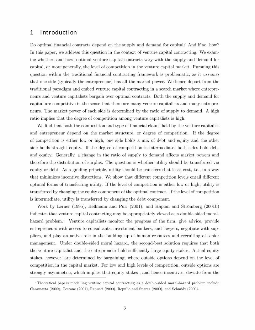
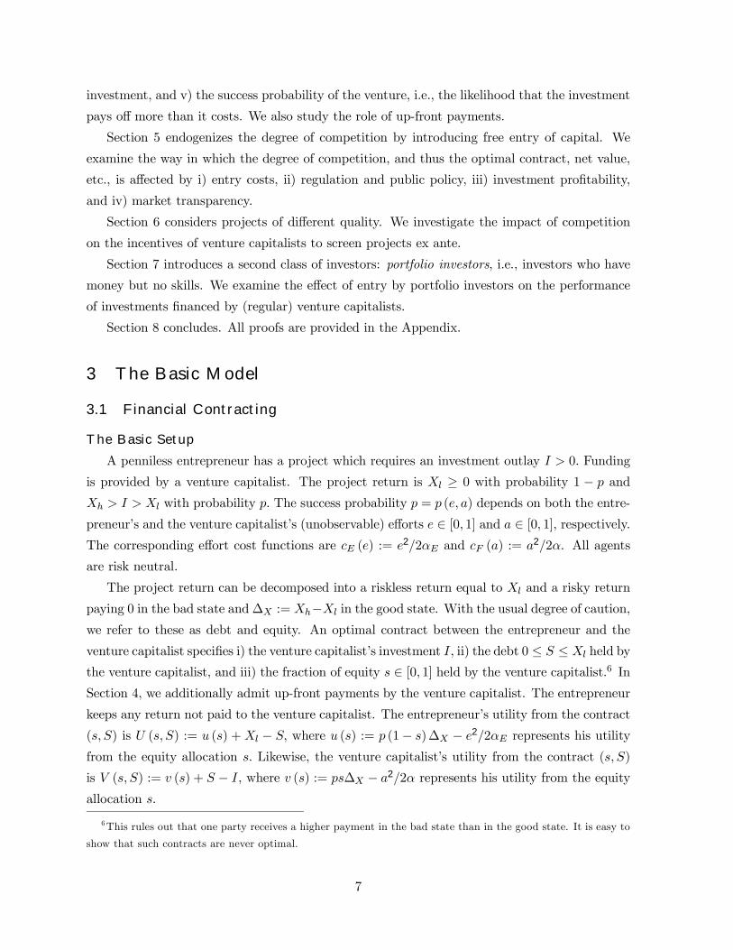
Figure 1: Equity Frontier for Linear Technology.

Figure 1 depicts the utility possibility frontier generated by different equity allocations. By

increasing the venture capitalist’s equity share s from zero to one, we move along the curve

clockwise. In the picture, we assume that αE (1− d)2 > αFd2, i.e., the entrepreneur is more

productive than the venture capitalist. If the reverse holds or if productivities are equal, the

picture looks similar. Appendix A discusses all cases.

The equity frontier is the undominated segment of the utility possibility frontier. It is defined

on the interval [v, v], where in this example v = v(0) = 0 and v = v(s), where s < 1. If s > s,

the utility of both parties decreases with s, which is due to the fact that the entrepreneur is

more productive. Hence, even if the venture capitalist had all the market power, he would want

to leave the entrepreneur some rent. (If the venture capitalist were more productive, the reverse

would hold.) A formal derivation of the equity frontier and a proof that properties i)−iii) holdis provided in Appendix A.

Example 2: Cobb-Douglas Technology. To ensure that the equilibrium success

probability has an interior solution, we assume again that max {αE (1− d) ,αFd} < 1/∆X .

Equilibrium effort choices are then e∗(s) = (αE (1− d) (1− s)∆X [a∗(s)]d)1

1+d and a∗(s) =

(αFds∆X [e∗(s)]1−d)

12−d , implying that

p∗ (s) = ρ (s)∆X , (4)

where ρ (s) := [αFds]d [αE(1− d)(1− s)]1−d . The venture capitalist’s and entrepreneur’s utility

from the equity allocation s is

v(s) =1

2(2− d) s∆2

Xρ (s) , (5)

9

and

u(s) =1

2(1 + d) (1− s)∆2

Xρ (s) . (6)

respectively.

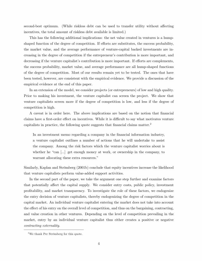
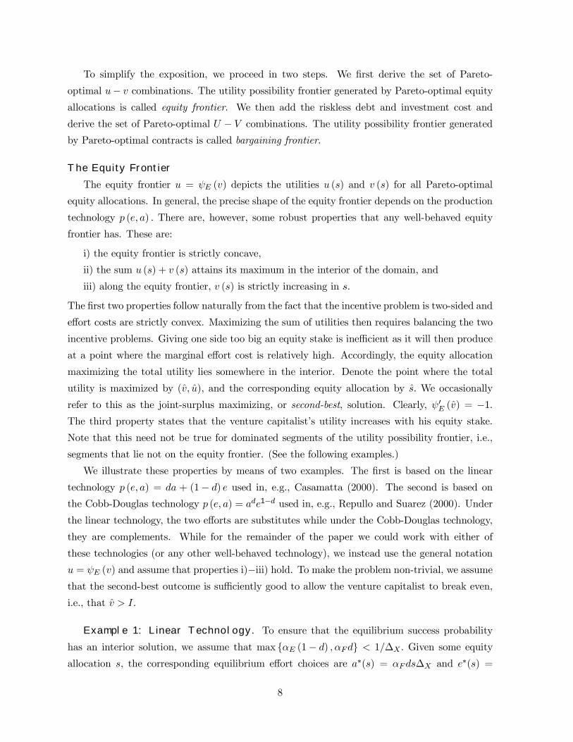
Figure 2: Equity Frontier for Cobb-Douglas Technology.

Figure 2 depicts the utility possibility and equity frontier for the Cobb-Douglas technology.

Since efforts are complements, only a relatively small segment of the utility possibility frontier

is undominated. In Appendix A we show that properties i)-iii) again hold.

The Bargaining Frontier

The bargaining frontier depicts the utility of the entrepreneur and venture capitalist, U =

u (s)+Xl−S and V = v (s)+S−I, respectively, for all Pareto-optimal contracts. We constructthe bargaining frontier from the equity frontier by adding the riskless debt in a way that mini-

mizes incentive distortions. (Adding the investment cost is trivial as it is borne by the venture

capitalist.) The construction is simple. Suppose s > s, in which case the venture capitalist holds

too much and the entrepreneur too little equity relative to the second-best. Any Pareto-optimal

contract where s > s must also have S = Xl, i.e., the venture capitalist must hold the entire

debt. If not, a Pareto-improvement would be possible where the entrepreneur trades in debt for

equity, thereby getting closer to the second-best solution. Similarly, if s < s, the entrepreneur

must hold the entire debt. If s = s, any debt allocation is Pareto-optimal.

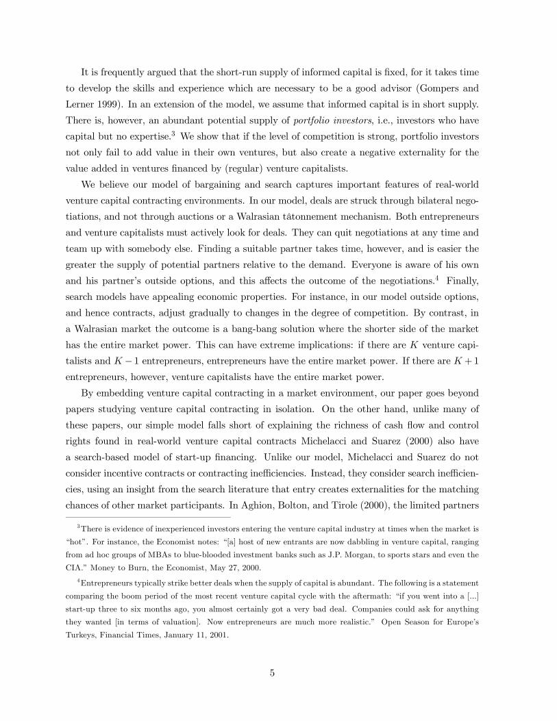
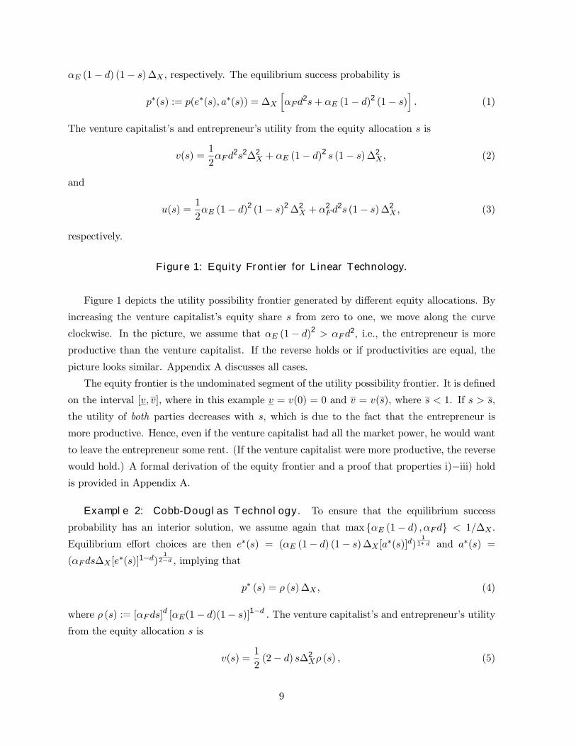
Figure 3: Construction of the Bargaining Frontier.

Figure 3 depicts the construction of the bargaining frontier. The figure is based on the equity

frontier in Figure 1. We therefore have v = 0, implying that max {v − I, 0} = 0. There are threeregions. In the left interval, the entrepreneur holds the entire debt and an inefficiently large

fraction of the equity. In the middle interval, both parties hold debt and equity. The equity

allocation is second-best optimal. As we move along the frontier clockwise, debt is shifted to

the venture capitalist until he holds all of it. As this is merely a wealth transfer, the slope of

the bargaining frontier in the middle interval is minus one. Finally, in the right interval, the

venture capitalist holds the entire debt and an inefficiently large fraction of the equity. This is

summarized in the following lemma.

Lemma 1. The bargaining frontier takes the following form:

U = ψB(V ) :=

ψE(V + I) +Xl if V ∈ [max {v − I, 0} , v − I]ψE(v) + [Xl − I + v − V ] if V ∈ [v − I, v +Xl − I]ψE(V −Xl + I) if V ∈ [v +Xl − I, v +Xl − I]

. (7)

10

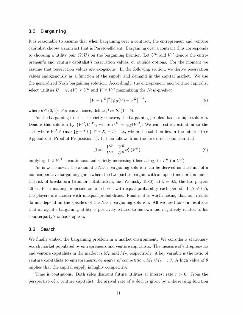
3.2 Bargaining

It is reasonable to assume that when bargaining over a contract, the entrepreneur and venture

capitalist choose a contract that is Pareto-efficient. Bargaining over a contract thus corresponds

to choosing a utility pair (V,U) on the bargaining frontier. Let UR and V R denote the entre-

preneur’s and venture capitalist’s reservation values, or outside options. For the moment we

assume that reservation values are exogenous. In the following section, we derive reservation

values endogenously as a function of the supply and demand in the capital market. We use

the generalized Nash bargaining solution. Accordingly, the entrepreneur and venture capitalist

select utilities U = ψB(V ) ≥ UR and V ≥ V R maximizing the Nash-product£V − V R¤b £ψB(V )− UR¤1−b , (8)

where b ∈ (0, 1) . For convenience, define β := b/ (1− b).As the bargaining frontier is strictly concave, the bargaining problem has a unique solution.

Denote this solution by¡V B, UB

¢, where UB = ψB(V

B). We can restrict attention to the

case where V B ∈ (max {v − I, 0} , v +Xl − I) , i.e., where the solution lies in the interior (seeAppendix B, Proof of Proposition 1). It then follows from the first-order condition that

β = −VB − V R

UB −URψ0B(V

B), (9)

implying that V B is continuous and strictly increasing (decreasing) in V R (in UR).

As is well known, the axiomatic Nash bargaining solution can be derived as the limit of a

non-cooperative bargaining game where the two parties bargain with an open time horizon under

the risk of breakdown (Binmore, Rubinstein, and Wolinsky 1986). If β = 0.5, the two players

alternate in making proposals or are chosen with equal probability each period. If β 6= 0.5,

the players are chosen with unequal probabilities. Finally, it is worth noting that our results

do not depend on the specifics of the Nash bargaining solution. All we need for our results is

that an agent’s bargaining utility is positively related to his own and negatively related to his

counterparty’s outside option.

3.3 Search

We finally embed the bargaining problem in a market environment. We consider a stationary

search market populated by entrepreneurs and venture capitalists. The measure of entrepreneurs

and venture capitalists in the market is ME and MF , respectively. A key variable is the ratio of

venture capitalists to entrepreneurs, or degree of competition, MF /ME =: θ. A high value of θ

implies that the capital supply is highly competitive.

Time is continuous. Both sides discount future utilities at interest rate r > 0. From the

perspective of a venture capitalist, the arrival rate of a deal is given by a decreasing function

11

q(θ), where limθ→0 q(θ) =∞ and limθ→∞ q(θ) = 0. Hence a venture capitalist is more likely to

meet an entrepreneur in a given time interval if the ratio of venture capitalists to entrepreneurs

is low. It is convenient to assume that q(θ) is continuously differentiable. Since the mass of deals

per unit of time is MEq(θ), the arrival rate of a deal from the perspective of an entrepreneur

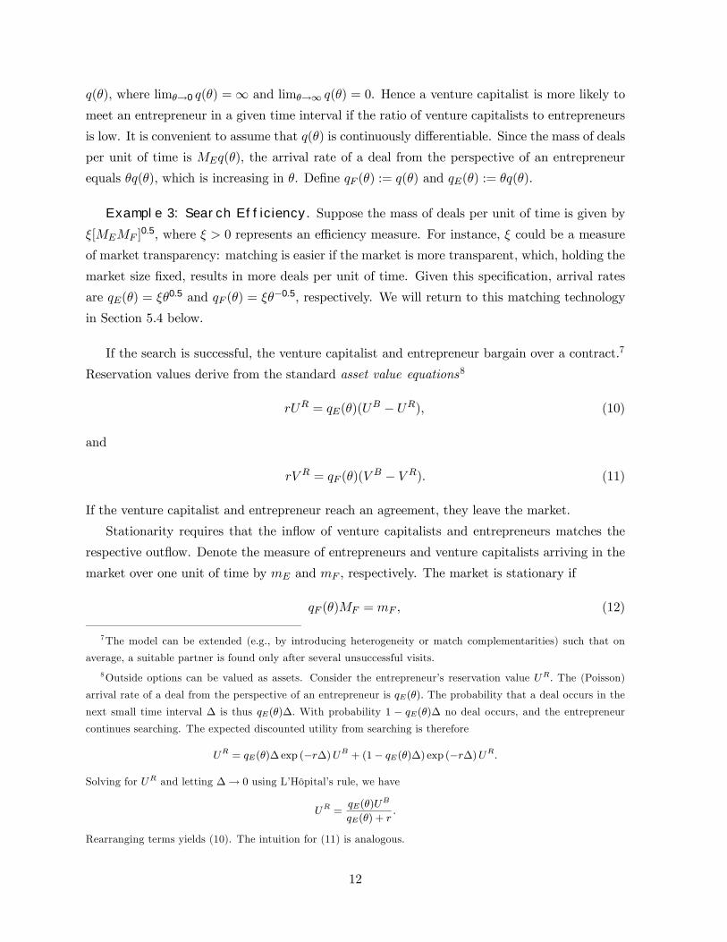
equals θq(θ), which is increasing in θ. Define qF (θ) := q(θ) and qE(θ) := θq(θ).

Example 3: Search Efficiency. Suppose the mass of deals per unit of time is given by

ξ[MEMF ]0.5, where ξ > 0 represents an efficiency measure. For instance, ξ could be a measure

of market transparency: matching is easier if the market is more transparent, which, holding the

market size fixed, results in more deals per unit of time. Given this specification, arrival rates

are qE(θ) = ξθ0.5 and qF (θ) = ξθ−0.5, respectively. We will return to this matching technology

in Section 5.4 below.

If the search is successful, the venture capitalist and entrepreneur bargain over a contract.7

Reservation values derive from the standard asset value equations8

rUR = qE(θ)(UB − UR), (10)

and

rV R = qF (θ)(VB − V R). (11)

If the venture capitalist and entrepreneur reach an agreement, they leave the market.

Stationarity requires that the inflow of venture capitalists and entrepreneurs matches the

respective outflow. Denote the measure of entrepreneurs and venture capitalists arriving in the

market over one unit of time by mE and mF , respectively. The market is stationary if

qF (θ)MF = mF , (12)

7The model can be extended (e.g., by introducing heterogeneity or match complementarities) such that on

average, a suitable partner is found only after several unsuccessful visits.

8Outside options can be valued as assets. Consider the entrepreneur’s reservation value UR. The (Poisson)

arrival rate of a deal from the perspective of an entrepreneur is qE(θ). The probability that a deal occurs in the

next small time interval ∆ is thus qE(θ)∆. With probability 1 − qE(θ)∆ no deal occurs, and the entrepreneur

continues searching. The expected discounted utility from searching is therefore

UR = qE(θ)∆ exp (−r∆)UB + (1− qE(θ)∆) exp (−r∆)UR.

Solving for UR and letting ∆→ 0 using L’Hôpital’s rule, we have

UR =qE(θ)U

B

qE(θ) + r.

Rearranging terms yields (10). The intuition for (11) is analogous.

12

and

qE(θ)ME = mE. (13)

As stationarity can always be ensured by scaling flows and stock accordingly, the market is fully

characterized by the ratio of venture capitalists to entrepreneurs θ.

We conclude by summarizing the equilibrium conditions.

Definition: Market Equilibrium. An equilibrium in the market with contracting, bar-

gaining, and search is defined by the following conditions.

i) Bargaining utilities¡V B, UB

¢maximize the Nash product (8).

ii) Reservation values¡V R, UR

¢satisfy the asset value equations (10)-(11).

iii) Flows (mE ,mF ) and stocks (ME ,MF ) satisfy the stationarity conditions (12)-(13).

To determine the equilibrium utilities V B, UB, V R, and UR, one must solve (9) and (10)-(11)

subject to UB = ψB(V B). Note that in the bargaining equation (9), the reservation values V R

and UR are exogenous, while in the asset value equations (10)-(11), the bargaining utilities V B

and UB are exogenous.

4 Results

4.1 Utilities, Financial Contracts, and Net Value Creation

Proposition 1 summarizes the main results. The key variable is the ratio of venture capitalists

to entrepreneurs, or degree of competition θ. For each θ, there exists a unique optimal contract,

unique bargaining utilities¡V B, UB

¢, and unique search utilitites

¡V R, UR

¢.

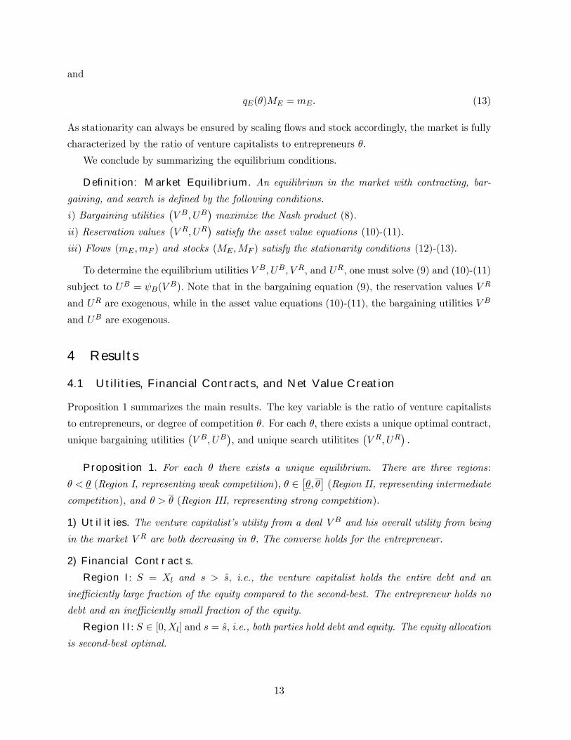
Proposition 1. For each θ there exists a unique equilibrium. There are three regions:

θ < θ (Region I, representing weak competition), θ ∈ £θ, θ¤ (Region II, representing intermediatecompetition), and θ > θ (Region III, representing strong competition).

1) Utilities. The venture capitalist’s utility from a deal V B and his overall utility from being

in the market V R are both decreasing in θ. The converse holds for the entrepreneur.

2) Financial Contracts.

Region I: S = Xl and s > s, i.e., the venture capitalist holds the entire debt and an

inefficiently large fraction of the equity compared to the second-best. The entrepreneur holds no

debt and an inefficiently small fraction of the equity.

Region II: S ∈ [0, Xl] and s = s, i.e., both parties hold debt and equity. The equity allocationis second-best optimal.

13

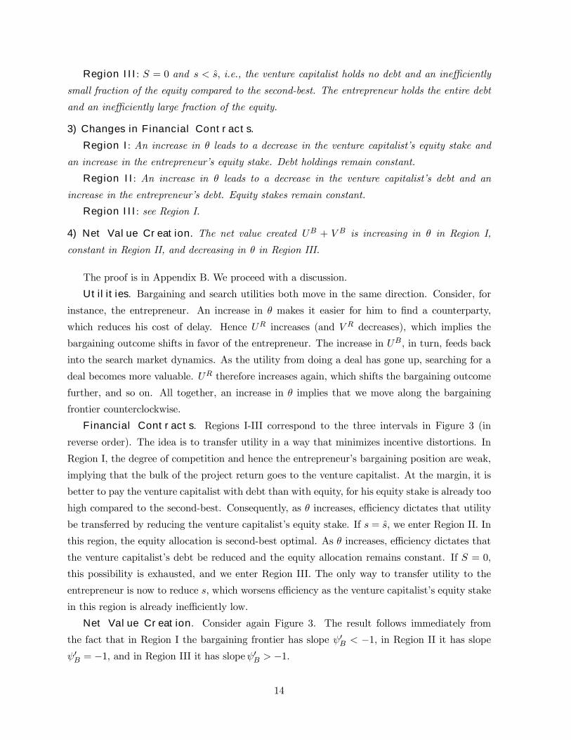
Region III: S = 0 and s < s, i.e., the venture capitalist holds no debt and an inefficiently

small fraction of the equity compared to the second-best. The entrepreneur holds the entire debt

and an inefficiently large fraction of the equity.

3) Changes in Financial Contracts.

Region I: An increase in θ leads to a decrease in the venture capitalist’s equity stake and

an increase in the entrepreneur’s equity stake. Debt holdings remain constant.

Region II: An increase in θ leads to a decrease in the venture capitalist’s debt and an

increase in the entrepreneur’s debt. Equity stakes remain constant.

Region III: see Region I.

4) Net Value Creation. The net value created UB + V B is increasing in θ in Region I,

constant in Region II, and decreasing in θ in Region III.

The proof is in Appendix B. We proceed with a discussion.

Utilities. Bargaining and search utilities both move in the same direction. Consider, for

instance, the entrepreneur. An increase in θ makes it easier for him to find a counterparty,

which reduces his cost of delay. Hence UR increases (and V R decreases), which implies the

bargaining outcome shifts in favor of the entrepreneur. The increase in UB, in turn, feeds back

into the search market dynamics. As the utility from doing a deal has gone up, searching for a

deal becomes more valuable. UR therefore increases again, which shifts the bargaining outcome

further, and so on. All together, an increase in θ implies that we move along the bargaining

frontier counterclockwise.

Financial Contracts. Regions I-III correspond to the three intervals in Figure 3 (in

reverse order). The idea is to transfer utility in a way that minimizes incentive distortions. In

Region I, the degree of competition and hence the entrepreneur’s bargaining position are weak,

implying that the bulk of the project return goes to the venture capitalist. At the margin, it is

better to pay the venture capitalist with debt than with equity, for his equity stake is already too

high compared to the second-best. Consequently, as θ increases, efficiency dictates that utility

be transferred by reducing the venture capitalist’s equity stake. If s = s, we enter Region II. In

this region, the equity allocation is second-best optimal. As θ increases, efficiency dictates that

the venture capitalist’s debt be reduced and the equity allocation remains constant. If S = 0,

this possibility is exhausted, and we enter Region III. The only way to transfer utility to the

entrepreneur is now to reduce s, which worsens efficiency as the venture capitalist’s equity stake

in this region is already inefficiently low.

Net Value Creation. Consider again Figure 3. The result follows immediately from

the fact that in Region I the bargaining frontier has slope ψ0B < −1, in Region II it has slopeψ0B = −1, and in Region III it has slopeψ0B > −1.

14

Perhaps the main insight to be taken away is that equity is used to transfer utility if the

level of competition is either low or high, while riskless debt is used to transfer utility if the

level of competition is intermediate. Accordingly, the equity component of venture capital

contracts should be relatively stable for intermediate competition levels, but vary substantially

with changes in competition if competition is either weak or strong. The opposite holds for the

debt component. In relative terms, Proposition 1 implies that the fraction of the entrepreneur’s

compensation consisting of debt is a U-shaped function of the competition level. Conversely, the

fraction of the venture capitalist’s compensation consisting of debt is a hump-shaped function

of the competition level.

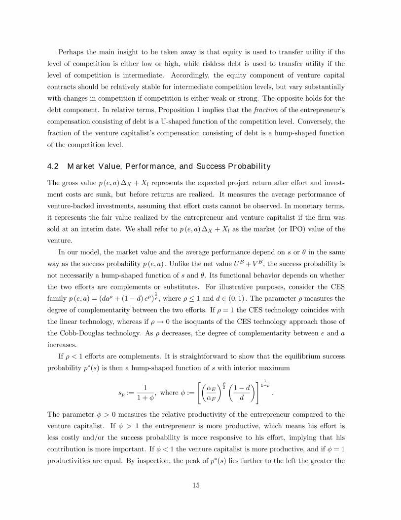
4.2 Market Value, Performance, and Success Probability

The gross value p (e, a)∆X +Xl represents the expected project return after effort and invest-

ment costs are sunk, but before returns are realized. It measures the average performance of

venture-backed investments, assuming that effort costs cannot be observed. In monetary terms,

it represents the fair value realized by the entrepreneur and venture capitalist if the firm was

sold at an interim date. We shall refer to p (e, a)∆X +Xl as the market (or IPO) value of the

venture.

In our model, the market value and the average performance depend on s or θ in the same

way as the success probability p (e, a) . Unlike the net value UB +V B, the success probability is

not necessarily a hump-shaped function of s and θ. Its functional behavior depends on whether

the two efforts are complements or substitutes. For illustrative purposes, consider the CES

family p (e, a) = (daρ + (1− d) eρ) 1ρ , where ρ ≤ 1 and d ∈ (0, 1) . The parameter ρ measures the

degree of complementarity between the two efforts. If ρ = 1 the CES technology coincides with

the linear technology, whereas if ρ→ 0 the isoquants of the CES technology approach those of

the Cobb-Douglas technology. As ρ decreases, the degree of complementarity between e and a

increases.

If ρ < 1 efforts are complements. It is straightforward to show that the equilibrium success

probability p∗(s) is then a hump-shaped function of s with interior maximum

sp :=1

1 + φ, where φ :=

"µαEαF

¶ρ2µ1− dd

¶# 11−ρ

.

The parameter φ > 0 measures the relative productivity of the entrepreneur compared to the

venture capitalist. If φ > 1 the entrepreneur is more productive, which means his effort is

less costly and/or the success probability is more responsive to his effort, implying that his

contribution is more important. If φ < 1 the venture capitalist is more productive, and if φ = 1

productivities are equal. By inspection, the peak of p∗(s) lies further to the left the greater the

15

entrepreneur’s productivity relative to that of the venture capitalist. If productivities are equal,

the peak is at sp = 1/2.

If ρ = 1 efforts are substitutes. We showed in Example 1 that the success probability

p∗(s) is then a monotonic function of s. If φ > 1 the function is strictly decreasing, while if

φ < 1 it is strictly increasing. If the entrepreneur is more productive, the success probability is

thus maximized at sp = 0. Conversely, if the venture capitalist is more productive, the success

probability is maximized at sp = 1. (This result can be obtained directly by maximizing (1)

with respect to s.)

To establish the relation between market value, average performance, and success probability

on the one side and competition on the other, recall that the venture capitalist’s equity stake

is a weakly decreasing function of θ, with a flat segment in Region II. Accordingly, if efforts

are complements the market value, average performance, and success probability are all hump-

shaped functions of the competition level (with a flat segment). On the other hand, if efforts are

substitutes they are either weakly increasing (if φ > 1) or weakly decreasing (if φ < 1) functions

of the competition level.

4.3 Up-front Payments

Suppose in addition to financing the investment cost I, the venture capitalist can make an up-

front payment P ∈ ¡0, P ¤ . (It is reasonable to assume that the entrepreneur cannot make anoteworthy up-front payment). Like riskless debt, up-front payments can be used to transfer

utility without affecting incentives. Consequently, the middle, i.e., linear, segment of the bar-

gaining frontier will extend to the left. There are two cases: if P ≥ v − I the left segmentvanishes completely. By contrast, if 0 < P < v − I all three segments of the bargaining frontierremain. The following result is then immediate.

Proposition 2. Suppose up-front payments can take values P ∈ ¡0, P ¤ .i) If P < v − I Proposition 1 holds as is. The middle segment of the bargaining fron-

tier is defined on V ∈ [v − I − P, v + Xl − I], while the leftmost segment is defined on

V ∈ [max©v − I − P, 0ª , v − I − P ].ii) If P ≥ v − I Region II extends to all θ ≥ θ, implying that Region III disappears. The

middle segment of the bargaining frontier is defined on V ∈ [0, v +Xl − I].

Introducing up-front payments has either no effect (P is small), or it causes Regions II and

III to collapse into a single region (P is large), which has the same properties as Region II.

From our perspective, what is important is that up-front payments have no effect on Region

I. As the venture capitalist’s equity stake in this region is inefficiently high, efficiency dictates

that utility be transferred by reducing his equity stake. Hence even if up-front payments are

16

possible, they will not be used. Introducing (potentially large) up-front payments therefore does

not affect our main conclusions: it is still true that for some competition levels equity is used

to transfer utility, while for others riskless debt (or up-front payments) is used. A change in the

level of competition continues to affect incentives, and thus the net value, success probability,

market value, and performance of venture-backed investments. Likewise, it still holds that for

some competition levels one side holds a mix of debt and equity and the other holds straight

equity, while for other competition levels both sides hold a mix. The literature appears to favor

the view that up-front payments should be small or even zero, however:

1) The promise to make up-front payments may attract a large pool of fraudulent entre-

preneurs, or “fly-by-night operators” (Rajan), who take the money and run (Rajan 1992, von

Thadden 1995. In the context of venture capital: Hellmann 2001). According to this argument,

up-front payments should be zero.

2) Up-front payments may be limited due to incentive problems between the venture capitalist

and his providers of capital (Holmström and Tirole 1997, Michelacci and Suarez 2000). To

mitigate the problem, the venture capitalist must put up a fraction of his own wealth, which

is arguably limited. Indeed, covenants in venture partnerships frequently require the “venture

capitalist to invest a set dollar amount or percentage in every investment made by the fund”

(Gompers and Lerner 1999, p. 40).

3) As the claims of limited partners in venture partnerships are senior, the claim of the

general partner (i.e., the venture capitalist) has features of a call option. To counteract risk-

taking by the venture capitalist, partnership agreements frequently include restrictions imposing

“a maximum percentage of capital invested in the fund [...] that can be invested in any one

firm” (Gompers and Lerner 1999, p. 38).

5 Endogenous Capital Supply

5.1 Closing the Model: Endogenous Entry

So far we have assumed that the degree of competition between venture capitalists is exogenous.

While this may be an adequate description of the market in the short run, the long-run supply

of venture capital is likely to be elastic. In what follows, we endogenize the supply side of

venture capital, thereby endogenizing the degree of competition in the market. This allows us

to study the relationship between venture capital contracts, the performance and value creation

of ventures, and various exogenous factors. The factors are entry costs, government subsidies

and regulation, investment profitability, and market transparency.

We take as given the flow of new ideas that are continuously created in the economy. Each

idea is associated with a single entrepreneur and cannot be traded. We normalize the flow of

17

new ideas such that the mass mE = 1 of ideas is created in the market over one unit of time.

The inflow of venture capital is determined by a zero-profit constraint. We assume that venture

capitalists entering the market incur entry costs k > 0, which may be conveniently thought of

as the cost of raising capital or acquiring information. Zero profit then implies that V R = k :

to recoup entry costs, venture capitalists must realize a positive utility in the market. While we

make the simplifying assumption that each venture capitalist can finance at most one project,

all our results hold if venture capitalists can finance a finite number of projects. The equilibrium

conditions are the same as before, except that mE = 1 and V R = k.

While it seems reasonable to assume that the supply of venture capital adjusts more quickly to

changes in exogenous parameters than the supply of new ideas, our model can be easily extended

to incorporate endogenous entry by both venture capitalists and entrepreneurs. Suppose, for

instance, that entrepreneurs face entry costs c ∈ [0, c]. These costs may, e.g., reflect initial R&Dor the cost of setting up a business plan. Otherwise all projects are identical. If c is sufficiently

large, there exists a threshold c < c such that only entrepreneurs with cost c ≤ c will enter themarket. This setup, in particular, generates the same results as the one considered here.

5.2 Financing Costs

In our model, venture capitalists face two costs of providing finance: entry costs k and investment

costs I. In what follows, we examine how changes in each of these costs affect the degree of

competition in the capital market.

Entry Costs

The venture capital industry is highly cyclical. In the past decades, there have been two

cycles: one starting in the late 1970s and ending in the late 1980s, the other starting in the

early 1990s. Each cycle witnessed entry by new venture capital funds: between 1991 and 1999

alone, the number of independent venture capital funds in the United States increased from 34

to 204. A factor potentially related to this massive entry of funds are changes in entry costs. As

more information about a technology or product becomes available, both the cost of information

acquisition and the uncertainty premium required by investors fall, implying that entry costs

decrease.

Consider the implications of a decrease in entry cost for the entry decision of venture cap-

italists.9 From the equality V R = k we have that V R must decrease by the same amount. By

Proposition 1, this implies that the degree of competition θ must rise.

Proposition 3. For each level of entry cost k, there exists a unique equilibrium. A decrease

9The market will only open up if venture capitalists can potentially break even, i.e., if v +Xl − I > k. We

assume that this holds.

18

in k corresponds to an increase in the level of competition θ and vice versa. The effects on

utilities and financial contracts are the same as in Proposition 1.

The proof is in Appendix B. Analogous to Proposition 1, there exist three regions: k > k

(Region I), k ∈ £k, k

¤(Region II), and k < k (Region III). In each region, the respective

statements from Proposition 1 hold. Among other things, this implies that the net value created

in ventures is a hump-shaped function of entry costs: if entry costs are high, there are too few

venture capitalists relative to the second-best. If entry costs are low, there are too many venture

capitalists. An individual venture capitalist entering the market does not take into account the

effect of his entry on the overall level of competition, and hence on the bargaining, contracting,

and value creation in other ventures. Entry by an individual venture capitalist therefore either

creates a positive (if there are too few venture capitalists) or negative (if there are too many)

contracting externality.

Regulation and Public Policy

In 1978 the United States abandoned the “prudent man rule”, a rule that prohibited pension

fund investments in securities issued by venture capital funds. The regulatory change was

accompanied by a cut in the capital gains tax from 49.5 to 28 percent. In 1981 taxes were

cut further to 20 percent.10 These changes triggered a surge in the supply of venture capital:

commitments to private equity partnerships during 1980-82 totaled more than $3.5 billion, two

and a half times the commitments to private equity during the entire decade of the 1970s.

Around the world, public programs have been designed to stimulate venture capital invest-

ment. In the United States, the bulk of these activities takes place on the state and local level

(Florida and Smith 1992). In Europe, the I-TEC project sponsored by the European Union

subsidizes initial (i.e., appraisal and management) costs, and the European Investment Fund

provides subsidized investment loans. The intention of these programs is not to replace, but to

stimulate the private provision of venture capital.

To examine the effect of investment subsidies, suppose they reduce the investment cost by

γI. As the venture capitalist’s investment outlay is now only (1− γ) I, fewer financial claims areneeded to make him break even. An increase in γ therefore either reduces the venture capitalist’s

equity stake s or his debt holdings S, whichever is more efficient.11 (If s > s a decrease in s is

more efficient, while if s ≤ s a decrease in S is more efficient).10Fenn, Liang, and Prowse (1995) provide a detailed account of the events.

11Technically, an increase in γ shifts the bargaining frontier to the right. There are two effects at work. First,

V B increases, implying that θ must increase since V R = k. Second, UB increases, implying that either s or S

must decrease. Both effects counteract the increase in γ, hence ensuring that V R = k.

19

Proposition 4. An investment subsidy γI has the same effect on financial contracts as an

(exogenous) increase in the degree of competition θ or a decrease in entry cost k.

The proof is in Appendix B. Of course, government can also directly subsidize or tax entry,

thereby changing entry costs. The effect is then as described in Proposition 3.

5.3 Investment Profitability

Another factor that might potentially trigger a positive influx of venture capital is an increase

in investment profitability. In our model, an increase in investment profitability can mean a

number of things: an increase in ∆X or Xl, or a decrease in I. In either case, the bargaining

frontier shifts outward. In what follows, we show that if an increase in profitability brings about

a change in the type of financial contract, i.e., if we move across the three regions in Proposition

1, the only possible direction is from Region I to Region II to Region III. This is the same

direction as in the case of an exogenous increase in the degree of competition θ or a decrease in

entry cost k. The result does not depend on the particular source of profitability increase.

The argument proceeds in two steps. First, it is reasonable to assume that the relative

importance of the entrepreneur’s and venture capitalist’s contribution does not change as the

investment becomes more profitable. Formally, this implies that the ratio of second-best utilities

v/u remains unchanged. Second, as the investment becomes more profitable, a smaller share of

the proceeds is needed to make the venture capitalist break even. As an illustration, suppose we

are in Region III where s < s and S = 0. The only way to reduce the venture capitalist’s share

of the proceeds is to reduce his equity stake s. As v/u is unchanged, this implies we must still

be in Region III, for moving to Region II or I would mean giving the venture capitalist more

equity. Similar arguments hold if we are in Regions I or II. The proof of the following result is

in Appendix B.

Proposition 5. Holding the ratio of second-best utilities v/u fixed, an increase in investment

profitability changes the type of financial contract in the same way as an (exogenous) increase

in the degree of competition θ or a decrease in entry cost k.

5.4 Market Transparency

So far we have studied changes affecting the costs and returns to financing. The market for

venture financing itself may undergo changes, however. In this section, we study how a change

in market transparency affects optimal financial contracts. We use the Cobb-Douglas matching

technology introduced in Example 3. According to this specification, the mass of new deals per

unit of time is ξ[MEMF ]0.5, where ξ > 0 is a measure of market transparency, or more generally,

market efficiency.

20

Consider first the case where the degree of competition θ is exogenous. Inserting the reser-

vation values (10)-(11) in the first-order condition for the Nash product (9), we obtain

βr + ξθ−

12

r + ξθ12

= −ψB(V B) V B

ψ(V B). (14)

Differentiating V B with respect to ξ while holding θ fixed shows that if θ < 1, i.e., if en-

trepreneurs outnumber venture capitalists, an increase in transparency increases the bargaining

utility of venture capitalists. Conversely, if θ > 1 an increase in transparency reduces V B.

Intuitively, the greater the market transparency, the stronger is the impact of competition, or

relative supply and demand, on the bargaining outcome. As this benefits the short side of

the market, its bargaining utility increases. Second, implicitly differentiating (9) reveals that

the cross-derivative of V B with respect to θ and ξ is negative. In words, the greater the mar-

ket transparency, the faster we move along the bargaining frontier as the level of competition

changes. Again, a greater market transparency amplifies the impact of market structure on the

bargaining outcome. To summarize, the effect of an exogenous change in θ on contracts and

utilities described in Proposition 1 is more pronounced the greater the market transparency.

In the case where entry is endogenous, the effect of transparency on the bargaining utilities

is ambiguous if θ < 1, but unambiguous if θ > 1. Consider, for instance, the effect on V B. There

are two effects. First, we know from the above discussion that an increase in transparency has a

positive effect on V B if θ < 1 and a negative effect if θ > 1. Second, an increase in transparency

reduces frictions and therefore the cost of delay. In principle, this implies that the venture

capitalist’s overall utility from being the market, V R, must rise. But V R cannot rise as it is

determined by the equality V R = k. To ensure that V R remains constant, the bargaining utility

V B must therefore decrease. Accordingly, there are two forces driving V B. If θ > 1 they move

in the same direction, whereas if θ < 1 they move in the opposite direction. This is summarized

in the following proposition. The proof is in Appendix B.

Proposition 6. If entry costs k are low (implying that θ > 1), an increase in market trans-

parency has the same effects on financial contracts and bargaining utilities as an (exogenous)

increase in the degree of competition θ or a decrease in entry cost k. If entry costs are high, the

effect is ambiguous.

6 Ex-Ante Project Screening

Thus far we have focused on two functions ascribed to venture capitalists: providing capital and

coaching projects. We now turn to a third, equally important function: separating good ideas

from bad ones. While entrepreneurs are always optimistic about their ideas, venture capitalists,

21

due to their experience and industry knowledge, are likely to have a better sense of whether a

given idea is workable or not. Suppose projects come in two qualities, or types: t ∈ T := {L,H}.The probability that a project (or entrepreneur) is of a high quality is π ∈ (0, 1] . Only high-quality projects are profitable. For simplicity, suppose a low-quality project yields a zero return

for sure. A priori, neither the venture capitalist nor the entrepreneur knows the project’s quality.

The venture capitalist can, however, learn it by screening the project. Screening comes at a cost

C > 0.

In what follows, we will argue that venture capitalists are less likely to screen projects if

the level of competition is strong. This is consistent with casual evidence that tapping venture

capital is easier in times when the venture capital market is booming.12 Before stating the result,

let us briefly lay out the argument. Each venture capitalist can finance and coach only a certain

number of projects. For simplicity, we assume in our model that this number is one. Before

sinking time and capital into a particular project, a venture capitalist will weigh the benefit

from doing so against the opportunity cost from (not) searching for a better candidate. If the

opportunity cost is high, the venture capitalist will carefully screen the project before making

the investment. If the opportunity cost if low, the benefits from screening are also low. Recall

that the utility from searching is V R. Since V R = k, we have that the venture capitalist is more

likely to screen if entry costs are high, or alternatively, if the degree of competition is low.

The sequence of moves is as follows. The venture capitalist and the entrepreneur bargain

over a contract which grants the venture capitalist the right to withdraw if he finds out that

the project is of low quality. Subsequently, the venture capitalist decides whether to screen or

not. If he screens, he learns the project quality for sure. If he does not screen, he holds prior

beliefs that he faces a high-quality project with probability π. If the venture capitalist does not

withdraw, he sinks the investment cost I. After the investment cost is sunk, the project quality

is fully revealed. The last assumption simplifies the analysis as it implies that effort choices are

made under complete information.

In a slight abuse of notation, denote the venture capitalist’s expected utility from investing

in a high-quality project by V B. If the venture capitalist screens and finds out that the quality

is low, it is optimal for him not to invest and to search anew. Moreover, as a low-quality project

generates a zero return, it does not pay an entrepreneur who has been rejected to stay in the

market.13 The expected utility from screening is then πV B + (1 − π)k − C. By contrast, theexpected utility from not screening is πV B − (1−π)I. Consequently, screening is optimal if and12See, e.g., Finance is a Siren Song, Financial Times, March 13, 2000.

13This rules out the existence of (negative) pool externalities. See Broecker (1990) for details.

22

only if

C ≤ (1− π)(k + I). (15)

From Proposition 3, we know that for each entry cost k there exists a unique corresponding

competition level θ. We thus have the following result.

Proposition 7. Ceteris paribus, screening is more likely if i) the cost of screening is low,

ii) the fraction of low-type projects is large, iii) the investment outlay (which is lost if a low-

quality project is financed) is large, and iv) entry cost k are high, or alternatively, the degree of

competition θ is low.

7 Portfolio Investors vs. Advisors

Gompers and Lerner (1999, p.4) point out that “[t]he skills needed for successful venture capital

investing are difficult and time-consuming to acquire. During periods when the supply or demand

for venture capital has shifted, adjustments in the number of venture capitalists and venture

capital organizations appear to take place very slowly.” The consequences of this are particular

apparent in boom periods such as the 1990s, where the demand for venture capital increased

sharply. In an attempt to fill the gap, an increasing number of new, inexperienced investors

entered the market.14 In this section, we model both the short-run stickiness of informed capital

and the entry by inexperienced investors who have money but no skills. We call the latter

portfolio investors.

Portfolio investors may be viewed as agents whose cost of providing effort is infinitely high. To

distinguish between regular venture capitalists and portfolio investors, we use the subscripts f ∈F := {A,P} , where A stands for advisor. There are two main differences between the bargainingfrontiers ψB,A and ψB,P . First, the fact that advisors add value while portfolio investors do not

shifts ψB,A outward relative to ψB,P . Second, unlike ψB,A, the bargaining frontier with portfolio

investors is strictly concave with slope ψ0B,P < −1 everywhere. As the moral hazard problemis only one-sided, efficiency dictates that portfolio investors hold as little equity as possible.

Accordingly, utility should be transferred by reducing the portfolio investor’s equity stake. The

bargaining frontier does not have a linear segment since the second-best allocation sP = 0 is not

feasible. (sP = 0 implies vP = 0, which in turn implies vP +Xl − I < 0.)As before, we assume that the mass mE = 1 of new ideas is created in the market over one

unit of time. We now additionally assume that over the same time period, the mass m < 1

14See, e.g., Banks Seek to Mine a Rich Seam: Private Equity, Financial Times, June 30, 2000, as well as the

reference in footnote 3.

23

of advisors arrives at the market fringe, where they must decide whether to enter or not.15

The inflow of portfolio capital is endogenous and determined by a zero-profit constraint. (The

formal equilibrium conditions, which extend the definitions in Sections 3.3 and 5.1, are stated

in Appendix C.) To ensure that portfolio investors can potentially break even, we assume that

vP +Xl − I > k . That is, the bargaining utility of portfolio investors under the most favorablebargaining outcome must be sufficiently large to cover the entry cost k. The following result

shows that Proposition 3 extends to multiple investor types. The proof is in Appendix C.

Proposition 8. For each entry cost k, there exists a unique equilibrium where both types

of investors enter. Analogous to Proposition 3, a decrease in k raises the level of competition

θ and reduces the bargaining utility of both advisors and portfolio investors. As for ventures

between entrepreneurs and advisors, the effect on financial contracts (and thus on incentives

and value creation) is the same as in Proposition 1. As for ventures between entrepreneurs and

portfolio investors, a decrease in k leads to a decrease in the portfolio investor’s equity stake and

an increase in the entrepreneur’s equity stake. The portfolio investor holds the entire debt, and

his debt holdings remain constant throughout.

Entry by an individual portfolio investor raises the overall level of competition. The extent

to which this entails a positive or negative (contracting) externality depends on whether we

consider ventures with advisors or portfolio investors. As for ventures between entrepreneurs

and portfolio investors, the externality is unambiguously positive. As competition increases,

utility is transferred to the entrepreneur by reducing the portfolio investor’s equity stake. Since

the moral hazard problem is one-sided, this improves efficiency. Also, both the market value and

the success probability increase. With regard to ventures between entrepreneurs and advisors,

the result is ambiguous. We showed in Section 5.2 that the externality is positive if competition

is weak but negative if competition is strong. In the latter case, entry by portfolio investors

reduces the net value in ventures financed by advisors and, provided efforts are complements,

also the market value and success probability in these ventures.

Being unskilled, portfolio investors have no advantage vis-a-vis advisors in our model. In

practice, this need not be the case. For instance, portfolio investors might have access to cheaper

funding, e.g., from in-house sources. On the other hand, advisors might have both better and

cheaper access to industry-specific information. In a young industry where the information

acquisition problem is important, advisors may thus face lower entry cost. By contrast, in a

mature industry portfolio investors may face lower entry costs. Given these assumptions, our

model has the following implication: as entry costs decrease and the relative cost advantage of

portfolio investors increases, advisors are driven out of the market. The reason for this is that i)

15 If m > 1, we are back to the previous setting. If m = 1, there exist multiple equilibria.

24

portfolio investors eventually face lower entry costs, and, more interestingly, ii) the increase in

competition and the associated negative contracting externality decrease the surplus produced

by advisors.

8 Concluding Remarks

Our paper yields numerous empirical predictions relating venture capital contracts, the intensity

of ex-ante project screening, and the value, success probability, and performance of venture-

backed investments to the relative supply and demand for venture capital (or degree of capital

market competition), entry costs, market transparency, investment profitability, and public pol-

icy. Most of these predictions remain yet to be tested. The ones that have been tested, however,

appear to be consistent with the empirical evidence. Perhaps the most crucial aspect of our

model is that the entrepreneur’s equity share increases with the level of competition (except

for intermediate levels, where it remains constant). This implies that incentives, the market

value, and the success probability of ventures all vary with the supply and demand for venture

capital. Indeed, Gompers and Lerner (2000) find that valuations are higher in times of strong

competition, which implies that the equity share of entrepreneurs increases as capital inflows and

competition among venture capitalists become more intense.16 The authors also examine the

relation between competition and the success of ventures. They find no statistically significant

difference for investments made during the late 1980s, a period when competition was strong,

and the early 1990s, a period of relatively low inflows. This is consistent with the hump-shaped

relation predicted by our model (if efforts are complements), which implies that the success rate

is low if competition is either strong or weak. It is, however, also consistent with the hypothesis

that there is no relation between competition and success. To discriminate between these two

hypotheses, more than two periods will be needed. Finally, Kaplan and Strömberg (2001a) find

that the entrepreneur’s equity share increases with investment performance, which is consistent

with the results stated in Proposition 5.

Our model can be extended in several directions. As it stands, the focus is on cash-flow

rights. Real-world venture capital contracts, however, include cash-flow rights, voting rights,

liquidation rights, board rights, and other instruments (Kaplan and Strömberg 2001a). One

conceivable extension is to examine how changes in competition affect the mix of different

contractual provisions. Again, the underlying principle must be that utility is transferred in a

way that minimizes incentive distortions. Second, we treat venture capitalists as a single entity.

In practice, venture capital partnerships consist of general and limited partners, which are tied

together by a contract. It would be interesting to analyze how competition simultaneously

16We thank Paul Gompers for bringing this to our attention.

25

affects both types of contracts, i.e., contracts between venture capitalists and entrepreneurs and

contracts between the general and limited partners. The question is whether the two contracts

move in the same or opposite direction.Third, we do not allow for project choice. Suppose there

is a choice between projects that rely heavily on the effort of venture capitalists and projects

that do not. If competition is strong and venture capitalists’ equity stakes are inefficiently small,

it will become optimal for venture capitalists to move away from effort-intensive activities such

as early-stage seed financing toward less effort-intensive activities.

9 Appendix

9.1 Appendix A: Specific Production Technologies

Example 1: Linear Technology. The equity frontier derives from the following program:

the entrepreneur choose s to maximize u (s) subject to the constraint that v (s) ≥ v. The solutionis characterized for all feasible reservation values v ≥ 0. (If v is too large, the solution is not

feasible). In a slight abuse of notation, we denote the solution by s∗(v). Both v(s) and u(s) are

strictly quasiconcave. Accordingly, s∗ is a solution to the entrepreneur’s problem if and only if

v(s) is nondecreasing and u(s) is nonincreasing at s∗. Define

s :=αFd

2 − αE (1− d)22αFd2 − αE (1− d)2

,

and

s :=αE (1− d)2

2αE (1− d)2 − αFd2,

where 0 < s < s < 1. We obtain the following result:

i) if αE (1− d)2 > αFd2, the set of Pareto-optimal equity allocations is [0, s] ,

ii) if αE (1− d)2 = αFd2, the set of Pareto-optimal equity allocations is [0, 1] , and

iii) if αE (1− d)2 < αFd2, the set of Pareto-optimal equity allocations is [s, 1] .

Case i) is the case discussed in the text where the entrepreneur is more productive. In case

i), define v := 0 and v =: v(s). In case ii), define v := 0 and v := v(1). Finally, in case iii), define

v := v(s) and v := v(1). For any v ∈ [v, v], the solution s∗(v) satisfies

v =1

2αFd

2 (s∗(v))2∆2X + αE (1− d)2 s∗(v) (1− s∗(v))∆2

X . (16)

Solving (16) for s∗(v), we obtain

s∗(v) =αE (1− d)2∆X −Φ³

2αE (1− d)2 − αFd2´∆X

, (17)

26

where Φ :=qα2E (1− d)4∆2

X − 2v(2αE (1− d)2 − αFd2). Clearly, s∗(v) is strictly increasing.

Inserting (17) in (3) generates the equity frontier ψE (v) . Differentiating ψE (v) twice with

respect to v, we have

d2ψE(v)

dv2= −Φ−3

·³αE (1− d)2 − αFd2

´2+ αE (1− d)2 αFd2

¸< 0.

To show that the sum of utilities v + ψE(v) attains its maximum in the interior of [v, v], we

compute the derivative of ψE (v) at the boundaries. In case i), we have ψ0E(v) = [αFd2 −

αE (1− d)2]/[αE (1− d)2] > −1 and limv→v ψ0E(v) = −∞. In case ii), we have ψ0E(v) = 0 andlimv→v ψ0E(v) = −∞. Finally, in case iii), we have ψ0E(v) = 0 and ψ0E(v) = −αFd2/[αFd

2 −αE (1− d)2] < −1. Since ψE(v) is strictly concave, this implies that in each case there exists aunique v ∈ (v, v) such that ψ0E (v) = −1. Q.E.D.

Example 2: Cobb-Douglas Technology. Again, v(s) and u(s) are both quasiconcave,

implying that s∗ solves the entrepreneur’s problem for some v if and only if v (s) is nondecreasing

and u (s) is nonincreasing at s∗. Differentiating (5) with respect to s, we have that v (s) is

nondecreasing if and only if s ≤ [1 + d]/2. Similarly, differentiating (6) with respect to s, we

have that u (s) is nonincreasing if and only if s ≥ d/2. Accordingly, the set of Pareto-optimalequity allocations is [d/2, [1 + d]/2], implying that v := v(d/2) and v := v([1 + d]/2). Moreover,

v (s) is strictly increasing for all s < [1 + d]/2, implying that s∗(v) is strictly increasing for all

v < v. We next show that ψE is strictly concave. Differentiating u(s) and v(s) twice, we obtain

d2ψE(v)

dv2= −1

2(1 + d)∆2

Xρ (s∗(v))

µ1

v0(s∗(v))

¶2

·µ

d

(s∗(v))2+

(1− d) (2s∗(v)− d)s∗(v) (1− s∗(v)) (1 + d− 2s∗(v))

¶,

which is strictly negative for all s∗ ∈ [d/2, (1 + d)/2]. To show that the sum of utilities v +

ψE(v) attains its maximum in the interior of [v, v], we compute the derivative of ψE (v) at the

boundaries. The derivative of ψE (v) is

dψE(v)

dv= −(1 + d) (2s

∗(v)− d) (1− s∗(v))s∗(v) (2− d) (1 + d− 2s∗(v)) . (18)

Evaluating (18) at v and v, we obtain ψ0E(v) = 0 and limv→v ψ0E(v) = −∞. Since ψE (v) isstrictly concave, this implies there exists a unique v ∈ (v, v) such that ψ0E (v) = −1. Q.E.D.

9.2 Appendix B: Proofs of Propositions 1 and 3-6

Proof of Proposition 1. To apply the first-order condition (9), we must first show that the

bargaining outcome lies in the interior of the domain of ψB. Given that V R ≥ 0 and UR ≥ 0,

27

there are only two possible cases where this might not hold: if v− I > 0 and ψ0B(v− I) < 0, andif ψB(v+Xl−I) > 0 and limV→v+Xl−I ψ

0B(V ) > −∞. To show that these cases cannot arise, we

argue to a contradiction. Suppose that v−I > 0 and ψ0B(v−I) < 0, implying that s∗(v) > 0. Butψ0E(v) = u

0(s∗)/v0(s∗), ψ0E(v) < 0, and Pareto optimality imply that u0(s∗(v)) < 0. Hence there

exists some equity allocation s < s∗(v) which makes the entrepreneur better off, contradicting

the construction of ψE , which requires that u (s) is maximized at s∗(v). An analogous argument

holds for the second case.

We next prove uniqueness. Inserting (10)-(11) into (9) yields

βr + qF (θ)

r + qE(θ)= −ψ0B(V B)

V B

ψB(V B). (19)

From the uniqueness of the bargaining solution, it follows that (19) has a unique solution

(UB, V B), where V B ∈ (0, v + Xl − I). As for claim 1), implicitly differentiating (19) with

respect to θ gives

dV B

dθ= β

[r + qF ] q0E − [r + qE ] q0F[r + qE ]

2

ψ2B

ψB£ψ0B + V Bψ

00B

¤− V B ¡ψ0B¢2 < 0,

implying that dUB/dθ > 0. This, in conjunction with the monotonicity of qE and qF , implies

that V R is decreasing and UR increasing in θ.

Claims 2)-3) follow now from the construction of the bargaining frontier and the monotonicity

of UB and V B. In particular, by (19), the threshold θ is uniquely determined by V B = v+Xl−I, while θ is uniquely determined by V B = bv − I. Q.E.D.

Proof of Proposition 3. In equilibrium, θ, UB, and V B are determined by (19) and the

zero-profit constraint V R = k. The total derivatives from these two equations generate the

following equation system: −β [r+qF ]q0E−[r+qE ]q0F[r+qE ]2

ψB[ψ0BV Bψ00B]−V B(ψ0B)2

ψ2B

V Brq0F

[qF+r]2qFqF+r

à dθ

dV B

!=

Ã0

1

!dk. (20)

The determinant of this system, D, is negative. In conjunction with the limit properties of

qF and qE for θ → 0 and θ →∞, this establishes the existence and uniqueness of a solution tothe equation system given by (19) and V R = k. We can now apply Cramer’s rule and obtain

dθ

dk= − 1

D

"−V B rq0F

[qF + r]2

ψB£ψ0B + V

Bψ00B¤− V B (ψ0B)2

ψ2B

#< 0.

The rest follows from Proposition 1. Q.E.D.

Proof of Proposition 4. An increase in γ shifts the bargaining frontier outward. (The

bargaining frontier is the same as in the basic model, except that I is replaced by ∆I :=

28

(1− γ)I.) Define ζ := ψ0B(V )/ψB(V ), and observe that dζ/d∆I < 0. (More precisely, dζ/d∆I =[ψBψ

00B − (ψ0B)2]/ψ2

B < 0 if V ≤ v − ∆I or V ≥ v + Xl − ∆I , and dζ/d∆I = ψ0B/ψ2B < 0 if

v −∆I ≤ v ≤ v +Xl −∆I .) In what follows, we show that dUB/d∆I < 0, which proves the

claim in the proposition.

We argue to a contradiction, assuming that UB is nondecreasing in ∆I for some ∆I . Inspec-

tion of the equilibrium conditions shows that this can only happen if θ is nondecreasing in ∆I .

However, from the equation system generated by the total derivatives of (19) and V R = k, we

have that

dθ

d∆I= − 1

DV B

dζ

d∆I

qFqF + r

< 0,

contradiction. Q.E.D.

Proof of Proposition 5. Proposition 4 considers a decrease in I. It therefore remains to

prove the result for an increase in ∆X and/or Xl. Take any two profitability levels L (low) and

H (high). We argue to a contradiction, assuming that an increase in profitability from L to H

induces a clockwise move across regions. The proof proceeds in two steps. We first show that

this must imply that

V BHUBH

<V BLUBL

. (21)

Recall that V RH = V RL = k. Suppose first that θH ≤ θL. From the zero-profit constraint V RH = k,

it follows that V BH ≤ V BL , implying UBH > UBL and therefore (21). Suppose next that θH > θL.

Moving clockwise across regions implies that

−ψ0B,H(V BH ) > −ψ0B,L(V BL ). (22)

Moreover, equations (9)-(11) imply that

−ψ0B,H(V BH )V BH

ψB,H(V BH )

r + qE(θH)

r + qF (θH)= −ψ0B,L(V BL )

V BLψB,L(V BL )

r + qE(θL)

r + qF (θL). (23)

Together, (22)-(23), θH > θL, and monotonicity of qE and qF , imply (21).

Having established that (21) must hold, we can now consider all possible moves across regions.

Suppose first we move from Region II or III to Region I. By the definition of Regions I-III, this

implies that

V BHUBH

>vH +Xl − I

uH, (24)

and

V BLUBL

≤ vL +Xl − IuL

. (25)

29

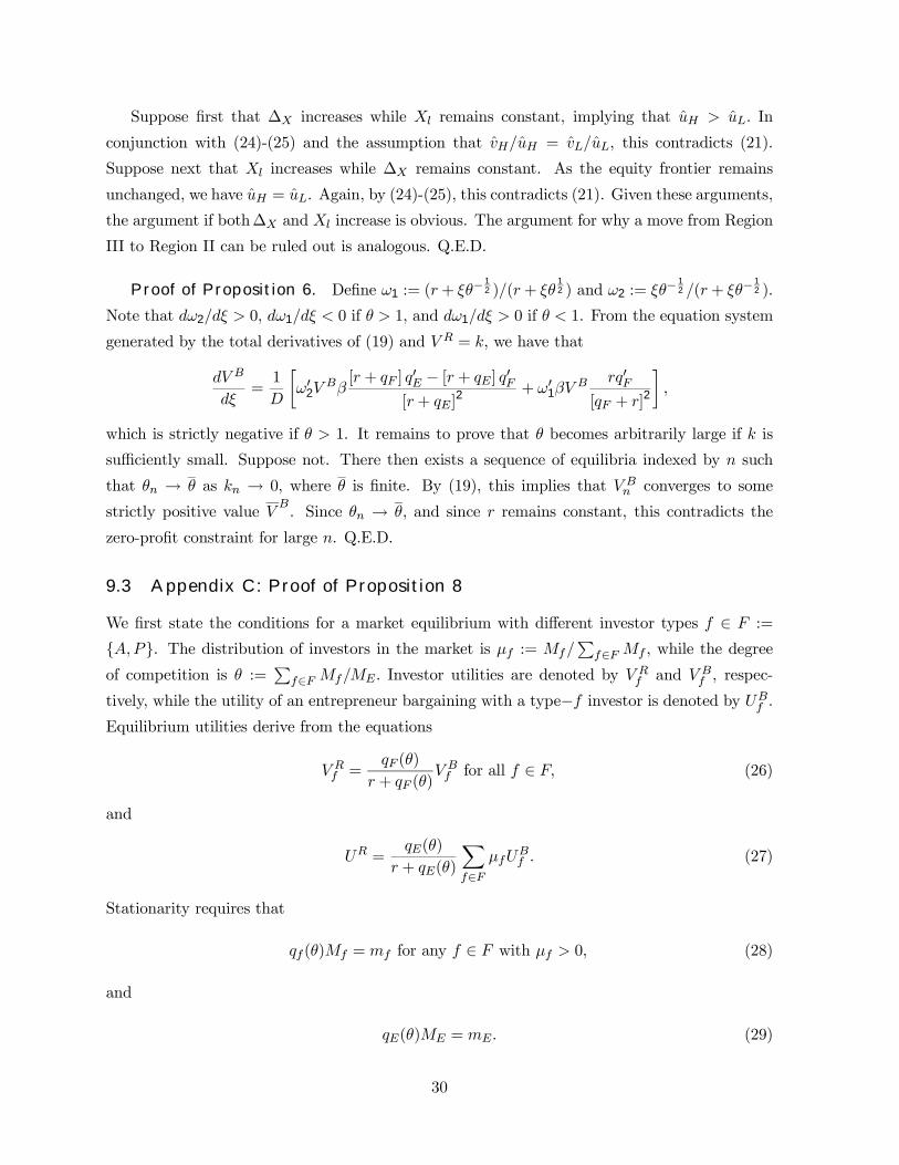
Suppose first that ∆X increases while Xl remains constant, implying that uH > uL. In

conjunction with (24)-(25) and the assumption that vH/uH = vL/uL, this contradicts (21).

Suppose next that Xl increases while ∆X remains constant. As the equity frontier remains

unchanged, we have uH = uL. Again, by (24)-(25), this contradicts (21). Given these arguments,

the argument if both∆X and Xl increase is obvious. The argument for why a move from Region

III to Region II can be ruled out is analogous. Q.E.D.

Proof of Proposition 6. Define ω1 := (r + ξθ−1

2 )/(r + ξθ12 ) and ω2 := ξθ

− 12 /(r + ξθ−

12 ).

Note that dω2/dξ > 0, dω1/dξ < 0 if θ > 1, and dω1/dξ > 0 if θ < 1. From the equation system

generated by the total derivatives of (19) and V R = k, we have that

dV B

dξ=1

D

·ω02V

Bβ[r + qF ] q

0E − [r + qE] q0F[r + qE]

2 + ω01βVB rq0F[qF + r]

2

¸,

which is strictly negative if θ > 1. It remains to prove that θ becomes arbitrarily large if k is

sufficiently small. Suppose not. There then exists a sequence of equilibria indexed by n such

that θn → θ as kn → 0, where θ is finite. By (19), this implies that V Bn converges to some

strictly positive value VB. Since θn → θ, and since r remains constant, this contradicts the

zero-profit constraint for large n. Q.E.D.

9.3 Appendix C: Proof of Proposition 8

We first state the conditions for a market equilibrium with different investor types f ∈ F :=

{A,P}. The distribution of investors in the market is µf := Mf/Pf∈F Mf , while the degree

of competition is θ :=Pf∈F Mf/ME . Investor utilities are denoted by V Rf and V Bf , respec-

tively, while the utility of an entrepreneur bargaining with a type−f investor is denoted by UBf .Equilibrium utilities derive from the equations

V Rf =qF (θ)

r + qF (θ)V Bf for all f ∈ F, (26)

and

UR =qE(θ)

r + qE(θ)

Xf∈F

µfUBf . (27)

Stationarity requires that

qf (θ)Mf = mf for any f ∈ F with µf > 0, (28)

and

qE(θ)ME = mE. (29)

30

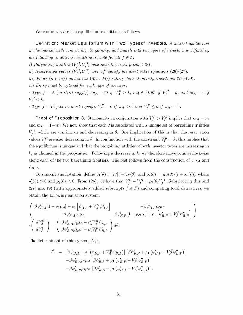
We can now state the equilibrium conditions as follows:

Definition: Market Equilibrium with Two Types of Investors. A market equilibrium

in the market with contracting, bargaining, and search with two types of investors is defined by

the following conditions, which must hold for all f ∈ F.i) Bargaining utilities (V Bf , U

Bf ) maximize the Nash product (8).

ii) Reservation values (V Rf , UR) and V Rf satisfy the asset value equations (26)-(27).

iii) Flows (mE ,mf ) and stocks (ME, Mf ) satisfy the stationarity conditions (28)-(29).

iv) Entry must be optimal for each type of investor :

- Type f = A (in short supply): mA = m if V RA > k, mA ∈ [0,m] if V RA = k, and mA = 0 if

V RA < k.

- Type f = P (not in short supply): V RP = k if mP > 0 and V RP ≤ k if mP = 0.

Proof of Proposition 8. Stationarity in conjunction with V RA > V RP implies that mA = m

andmE = 1−m. We now show that each θ is associated with a unique set of bargaining utilitiesV Bf , which are continuous and decreasing in θ. One implication of this is that the reservation

values V Rf are also decreasing in θ. In conjunction with the constraint V RP = k, this implies that

the equilibrium is unique and that the bargaining utilities of both investor types are increasing in

k, as claimed in the proposition. Following a decrease in k, we therefore move counterclockwise

along each of the two bargaining frontiers. The rest follows from the construction of ψB,A and

ψB,P .

To simplify the notation, define ρ1(θ) := r/[r+ qF (θ)] and ρ2(θ) := qE(θ)/[r+ qF (θ)], where

ρ01(θ) > 0 and ρ02(θ) < 0. From (26), we have that V Bf − V Rf = ρ1(θ)VBf . Substituting this and

(27) into (9) (with appropriately added subscripts f ∈ F ) and computing total derivatives, weobtain the following equation system: βψ0B,A [1− ρ2µA] + ρ1

hψ0B,A + V

BA ψ

00B,A

i−βψ0B,Pρ2µP

−βψ0B,Aρ2µA βψ0B,P [1− ρ2µP ] + ρ1

hψ0B,P + V

BP ψ

00B,P

i ·ÃdV BA

dV BP

!=

Ãβψ0B,Aρ

02µA − ρ01V BA ψ0B,A

βψ0B,Pρ02µP − ρ01V BP ψ0B,P

!dθ.

The determinant of this system, eD, iseD =

£βψ0B,A + ρ1

¡ψ0B,A + V

BA ψ

00B,A

¢¤ £βψ0B,P + ρ1

¡ψ0B,P + V

BP ψ

00B,P

¢¤−βψ0B,Aρ2µA

£βψ0B,P + ρ1

¡ψ0B,P + V

BP ψ

00B,P

¢¤−βψ0B,Pρ2µP

£βψ0B,A + ρ1

¡ψ0B,A + V

BA ψ

00B,A

¢¤.

31

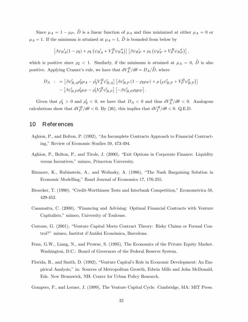
Since µA = 1 − µP , eD is a linear function of µA and thus minimized at either µA = 0 or

µA = 1. If the minimum is attained at µA = 1, eD is bounded from below by£βψB

0A(1− ρ2) + ρ1

¡ψB

0A + V

BA ψB

00A

¢¤ £βψB

0P + ρ1

¡ψB

0P + V

BP ψB

00P

¢¤,

which is positive since ρ2 < 1. Similarly, if the minimum is attained at µA = 0, eD is also

positive. Applying Cramer’s rule, we have that dV BA /dθ = DA/ eD, whereDA : =

£βψ0B,Aρ

02µA − ρ01V BA ψ0B,A

¤ £βψ0B,P (1− ρ2µP ) + ρ

¡1ψ

0B,P + V

BP ψ

00B,P

¢¤− £βψ0B,Pρ02µP − ρ01V BP ψ0B,P ¤ £−βψ0B,Pρ2µP

¤.

Given that ρ01 > 0 and ρ02 < 0, we have that DA < 0 and thus dV BA /dθ < 0. Analogous

calculations show that dV BP /dθ < 0. By (26), this implies that dVRf /dθ < 0. Q.E.D.

10 References

Aghion, P., and Bolton, P. (1992), “An Incomplete Contracts Approach to Financial Contract-

ing,” Review of Economic Studies 59, 473-494.

Aghion, P., Bolton, P., and Tirole, J. (2000), “Exit Options in Corporate Finance: Liquidity

versus Incentives,” mimeo, Princeton University.

Binmore, K., Rubinstein, A., and Wolinsky, A. (1986), “The Nash Bargaining Solution in

Economic Modelling,” Rand Journal of Economics 17, 176-255.

Broecker, T. (1990), “Credit-Worthiness Tests and Interbank Competition,” Econometrica 58,

429-452.

Casamatta, C. (2000), “Financing and Advising: Optimal Financial Contracts with Venture

Capitalists,” mimeo, University of Toulouse.

Cestone, G. (2001), “Venture Capital Meets Contract Theory: Risky Claims or Formal Con-

trol?” mimeo, Institut d’Anàlisi Económica, Barcelona.

Fenn, G.W., Liang, N., and Prowse, S. (1995), The Economics of the Private Equity Market.

Washington, D.C.: Board of Governors of the Federal Reserve System.

Florida, R., and Smith, D. (1992), “Venture Capital’s Role in Economic Development: An Em-

pirical Analysis,” in: Sources of Metropolitan Growth, Edwin Mills and John McDonald,

Eds. New Brunswick, NH: Center for Urban Policy Research.

Gompers, P., and Lerner, J. (1999), The Venture Capital Cycle. Cambridge, MA: MIT Press.

32

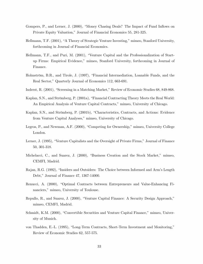
Gompers, P., and Lerner, J. (2000), “Money Chasing Deals? The Impact of Fund Inflows on

Private Equity Valuation,” Journal of Financial Economics 55, 281-325.

Hellmann, T.F. (2001), “A Theory of Strategic Venture Investing,” mimeo, Stanford University,

forthcoming in Journal of Financial Economics.

Hellmann, T.F., and Puri, M. (2001), “Venture Capital and the Professionalization of Start-

up Firms: Empirical Evidence,” mimeo, Stanford University, forthcoming in Journal of

Finance.

Holmström, B.R., and Tirole, J. (1997), “Financial Intermediation, Loanable Funds, and the

Real Sector,” Quarterly Journal of Economics 112, 663-691.

Inderst, R. (2001), “Screening in a Matching Market,” Review of Economic Studies 68, 849-868.

Kaplan, S.N., and Strömberg, P. (2001a), “Financial Contracting Theory Meets the Real World:

An Empirical Analysis of Venture Capital Contracts,” mimeo, University of Chicago.

Kaplan, S.N., and Strömberg, P. (2001b), “Characteristics, Contracts, and Actions: Evidence

from Venture Capital Analyses,” mimeo, University of Chicago.

Legros, P., and Newman, A.F. (2000), “Competing for Ownership,” mimeo, University College

London.

Lerner, J. (1995), “Venture Capitalists and the Oversight of Private Firms,” Journal of Finance

50, 301-318.

Michelacci, C., and Suarez, J. (2000), “Business Creation and the Stock Market,” mimeo,

CEMFI, Madrid.

Rajan, R.G. (1992), “Insiders and Outsiders: The Choice between Informed and Arm’s Length

Debt,” Journal of Finance 47, 1367-14000.

Renucci, A. (2000), “Optimal Contracts between Entrepreneurs and Value-Enhancing Fi-

nanciers,” mimeo, University of Toulouse.

Repullo, R., and Suarez, J. (2000), “Venture Capital Finance: A Security Design Approach,”

mimeo, CEMFI, Madrid.

Schmidt, K.M. (2000), “Convertible Securities and Venture Capital Finance,” mimeo, Univer-

sity of Munich.

von Thadden, E.-L. (1995), “Long-Term Contracts, Short-Term Investment and Monitoring,”

Review of Economic Studies 62, 557-575.

33

�

�

��� ����� ���

�� �� � ������� �� ���

!"#$%

� &(' ) * +

�

�

��� ����� ���

�� �� � ��� ���� �� ���

� ! " #

$%&'(

�

�

� � � ����� ���

��� �������������������

�

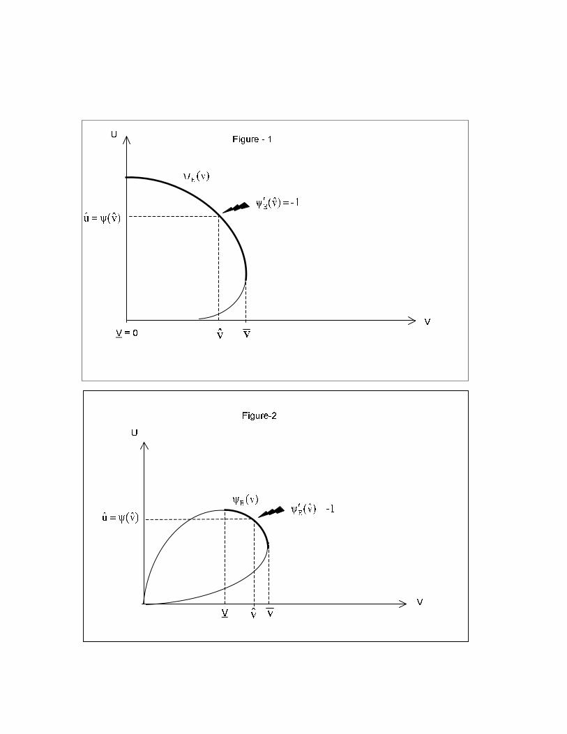
!" # $ %&' ( )+*,-./ 0 12

34

5

34