1

Velsto 1.2.1 Installation and User instructions.

Raafcom B.V. Feb 2013 ,updated nov 2017

(raafcom@gmail.com)

(This document is stored by the installer in c:\data\Velsto\docs)

Introduction. Velsto is an Open Source program for determining average depth and standard deviation depth of a

set of time horizons based on Gaussian Simulation using a layer cake model. To convert from time to

depth various velocity models can be specified. To tie the simulation results to wells there is a

residuals workflow where proper QA/QC of markers/residuals can be done and kriged maps can be

produced. Gridding and a basic Grid Calculator using GMT routines are included.

Velsto has been developed by Raafcom B.V. located in Assen The Netherlands. The functionality is

based on advice from geophysicists, knowledge from 31 years in subsurface IT and on publicly

available literature(see references).

Velsto 1.2.1 is an intermediate release after v1.2 with a new Grid calculator and a Control points

calculator. It is the plan to develop Velsto further the coming years, any suggestions are welcome.

In Velsto use is made of third party Open source programs/libraries.

Mapwindow GIS (www.mapwindow.org). (Mapping + Variogram + Grid Calculator)

GSLIB Geostatistical Library (www.gslib.com). (Kriging)

GMT Generic Mapping Tool. (www.soest.hawaii.edu/gmt). (Gridding)

References.

Characterization of the Structural uncertainty in the case of a South-Hungarian HC-reservoir,

Peter Zahuczki, MOL Plc May 2007.

(www.peter.zahuczki.hu).

3D Subsurface mapping of the Dutch offshore Results and Progress. Serge van Gessel, Hans

Doornenbal, Ed Duin, Nora Witmans ,TNO Bouw en Ondergrond, June 2008.

(www.tno.nl/downloads/InFormation20-art4.pdf).

Support. Support of Velsto is given on a best effort basis. Send an email to raafcom@gmail.com with

queries,bugs,suggestions and you will be replied within 24 hours.

2

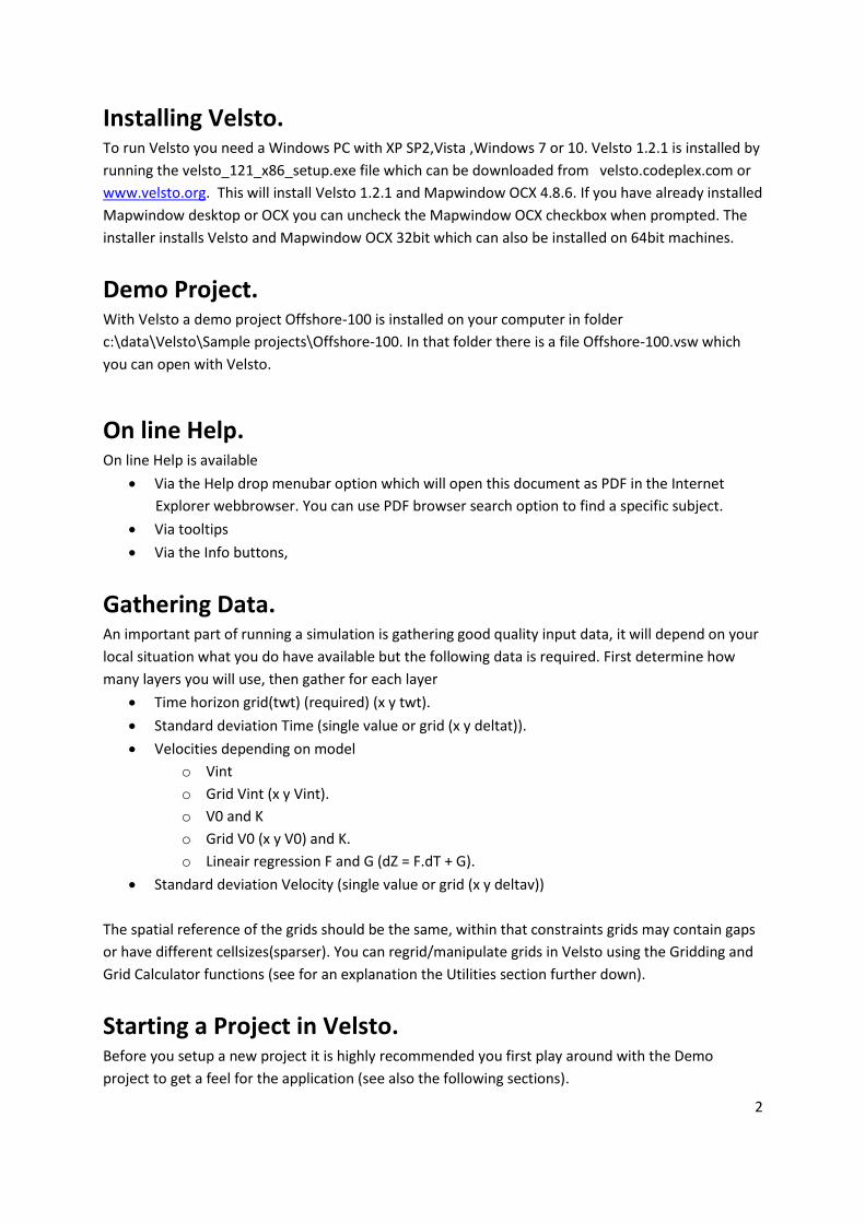
Installing Velsto. To run Velsto you need a Windows PC with XP SP2,Vista ,Windows 7 or 10. Velsto 1.2.1 is installed by

running the velsto_121_x86_setup.exe file which can be downloaded from velsto.codeplex.com or

www.velsto.org. This will install Velsto 1.2.1 and Mapwindow OCX 4.8.6. If you have already installed

Mapwindow desktop or OCX you can uncheck the Mapwindow OCX checkbox when prompted. The

installer installs Velsto and Mapwindow OCX 32bit which can also be installed on 64bit machines.

Demo Project. With Velsto a demo project Offshore-100 is installed on your computer in folder

c:\data\Velsto\Sample projects\Offshore-100. In that folder there is a file Offshore-100.vsw which

you can open with Velsto.

On line Help. On line Help is available

Via the Help drop menubar option which will open this document as PDF in the Internet

Explorer webbrowser. You can use PDF browser search option to find a specific subject.

Via tooltips

Via the Info buttons,

Gathering Data. An important part of running a simulation is gathering good quality input data, it will depend on your

local situation what you do have available but the following data is required. First determine how

many layers you will use, then gather for each layer

Time horizon grid(twt) (required) (x y twt).

Standard deviation Time (single value or grid (x y deltat)).

Velocities depending on model

o Vint

o Grid Vint (x y Vint).

o V0 and K

o Grid V0 (x y V0) and K.

o Lineair regression F and G (dZ = F.dT + G).

Standard deviation Velocity (single value or grid (x y deltav))

The spatial reference of the grids should be the same, within that constraints grids may contain gaps

or have different cellsizes(sparser). You can regrid/manipulate grids in Velsto using the Gridding and

Grid Calculator functions (see for an explanation the Utilities section further down).

Starting a Project in Velsto. Before you setup a new project it is highly recommended you first play around with the Demo

project to get a feel for the application (see also the following sections).

3

A new project is started via File->New.

In the General Tab

enter a Project name (name may not contain spaces or backslashes).

Create a folder where to store result files and intermediate files (e.g. a subfolder of the

location where your input data is stored)

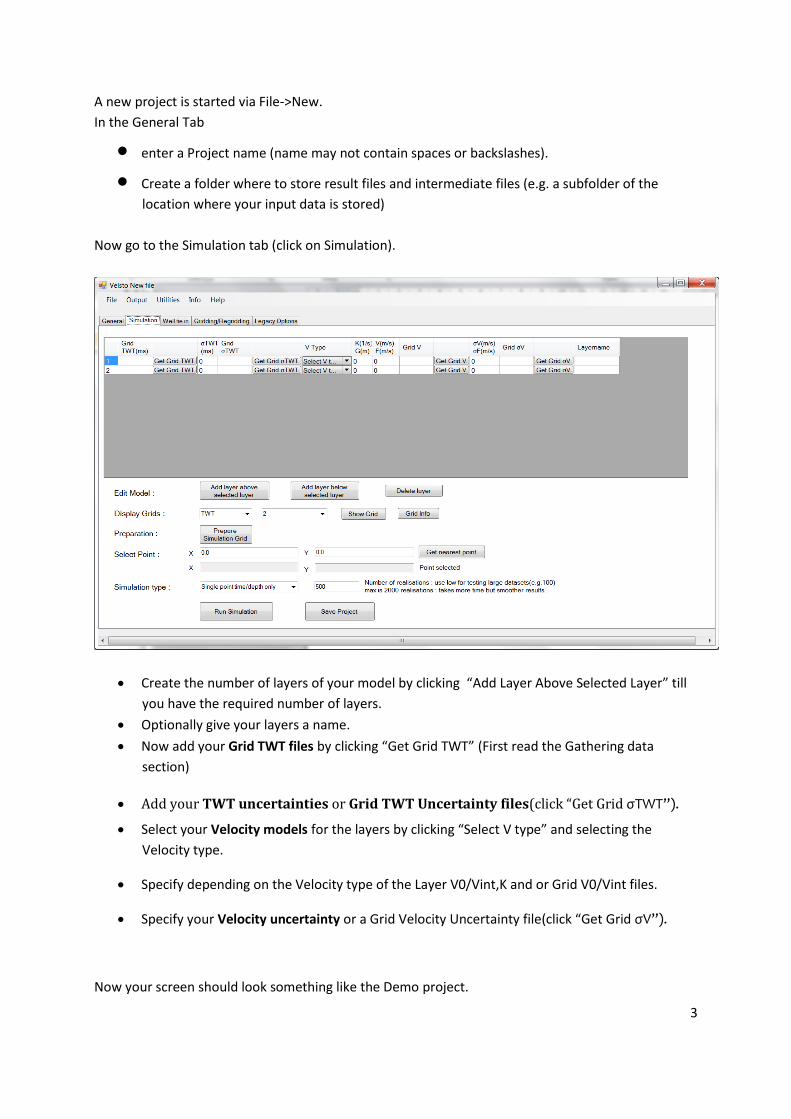
Now go to the Simulation tab (click on Simulation).

Create the number of layers of your model by clicking “Add Layer Above Selected Layer” till

you have the required number of layers.

Optionally give your layers a name.

Now add your Grid TWT files by clicking “Get Grid TWT” (First read the Gathering data

section)

Add your TWT uncertainties or Grid TWT Uncertainty files(click “Get Grid σTWT”).

Select your Velocity models for the layers by clicking “Select V type” and selecting the

Velocity type.

Specify depending on the Velocity type of the Layer V0/Vint,K and or Grid V0/Vint files.

Specify your Velocity uncertainty or a Grid Velocity Uncertainty file(click “Get Grid σV”).

Now your screen should look something like the Demo project.

4

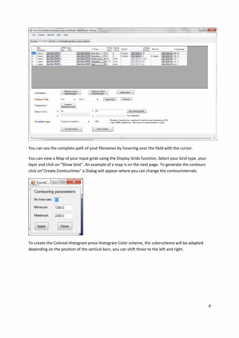
You can see the complete path of yout filenames by hovering over the field with the cursor.

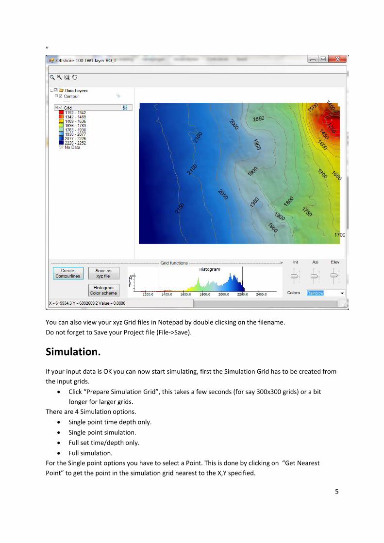
You can view a Map of your input grids using the Display Grids function. Select your Grid type, your

layer and click on “Show Grid”. An example of a map is on the next page. To generate the contours

click on“Create Contourlines” a Dialog will appear where you can change the contourintervals

To create the Colored Histogram press Histogram Color scheme, the colorscheme will be adapted

depending on the position of the vertical bars, you can shift those to the left and right.

5

”

You can also view your xyz Grid files in Notepad by double clicking on the filename.

Do not forget to Save your Project file (File->Save).

Simulation.

If your input data is OK you can now start simulating, first the Simulation Grid has to be created from

the input grids.

Click “Prepare Simulation Grid”, this takes a few seconds (for say 300x300 grids) or a bit

longer for larger grids.

There are 4 Simulation options.

Single point time depth only.

Single point simulation.

Full set time/depth only.

Full simulation.

For the Single point options you have to select a Point. This is done by clicking on “Get Nearest

Point” to get the point in the simulation grid nearest to the X,Y specified.

6

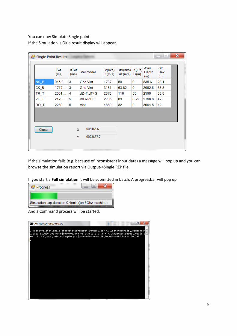
You can now Simulate Single point.

If the Simulation is OK a result display will appear.

If the simulation fails (e.g. because of inconsistent input data) a message will pop up and you can

browse the simulation report via Output->Single REP file.

If you start a Full simulation it will be submitted in batch. A progressbar will pop up

And a Command process will be started.

7

Once the Simulation is finished (the Command process and progress bar disappear from the screen

and a message appears) you can check the Simulation report via Output->Rep File.

You can view the resulting depths and standard deviation depth grids by selectiong with Display Grids

Z or σZ and the appropriate layer and clicking “Show Grid”

The results are stored in files <Projectname>.AVZ and <Projectname>.SDZ. (format x y z_layer1

z_layer2…. z_layer_n).

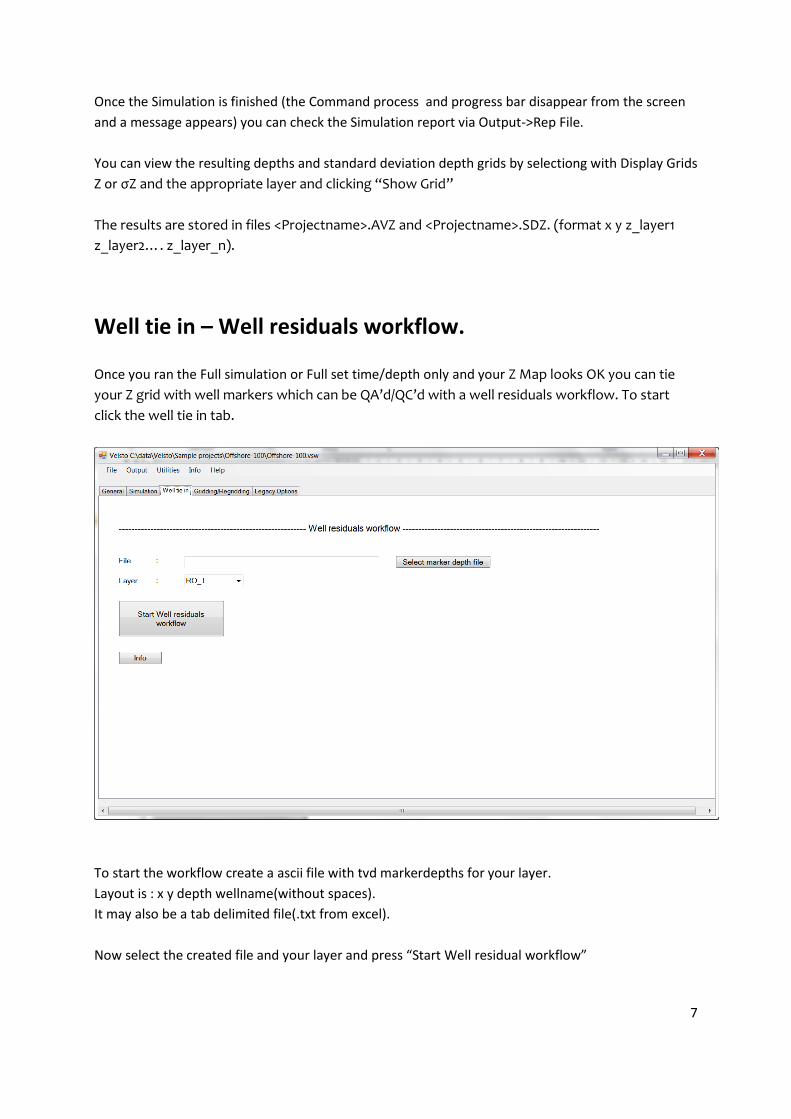
Well tie in – Well residuals workflow.

Once you ran the Full simulation or Full set time/depth only and your Z Map looks OK you can tie

your Z grid with well markers which can be QA’d/QC’d with a well residuals workflow. To start

click the well tie in tab.

To start the workflow create a ascii file with tvd markerdepths for your layer.

Layout is : x y depth wellname(without spaces).

It may also be a tab delimited file(.txt from excel).

Now select the created file and your layer and press “Start Well residual workflow”

8

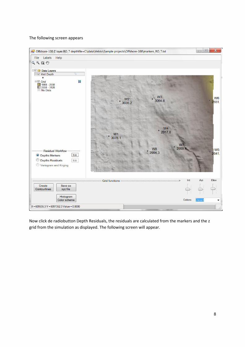
The following screen appears

Now click de radiobutton Depth Residuals, the residuals are calculated from the markers and the z

grid from the simulation as displayed. The following screen will appear.

9

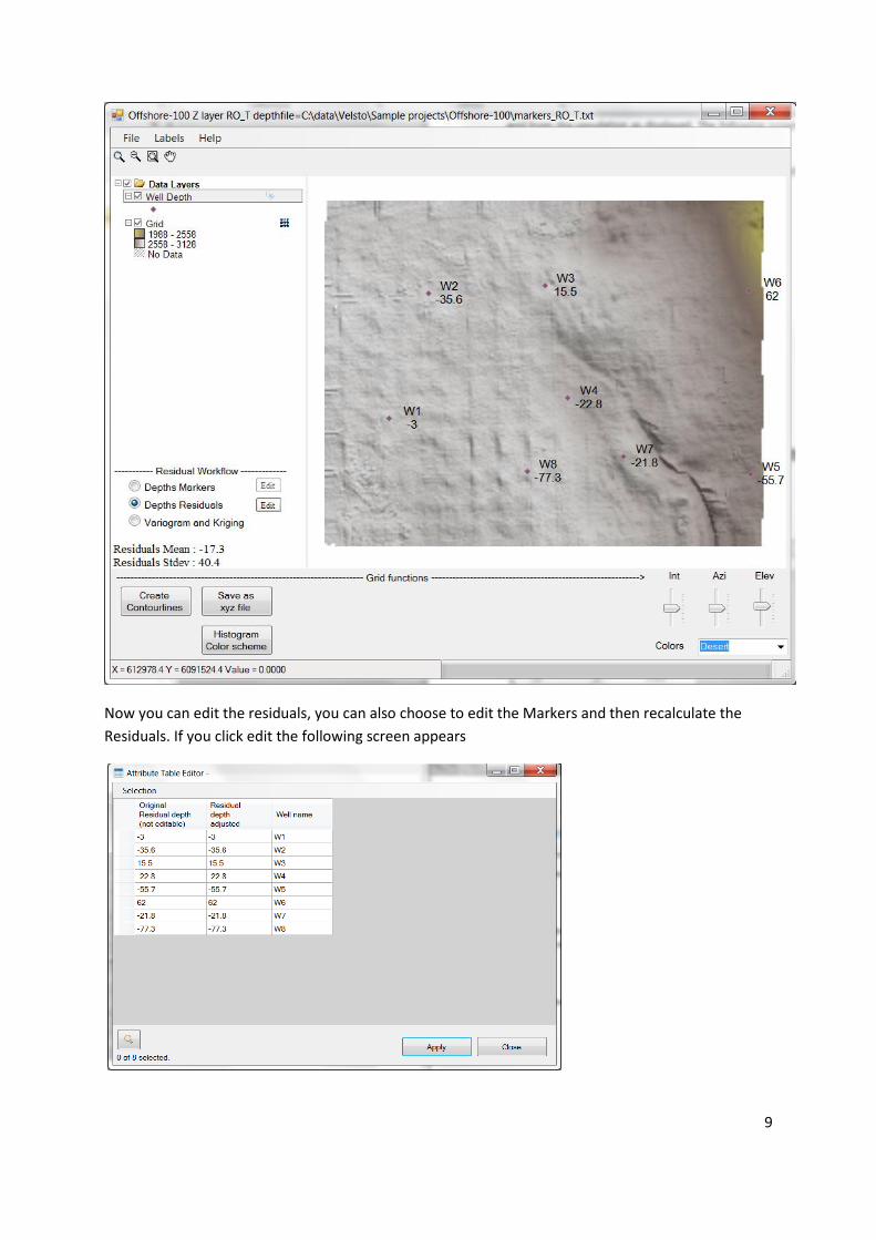
Now you can edit the residuals, you can also choose to edit the Markers and then recalculate the

Residuals. If you click edit the following screen appears

10

Here you can edit the depths(press Apply to update the map), close this window and save the

residuals using File->Save which will save the depths in a format with original and adjusted depths

and some header info. To ignore a point set the marker depth to 99999.

Alternatively you can edit the Markers and save them and recalculate the Residuals.

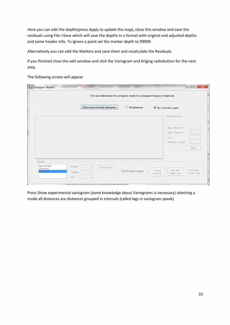
If you finished close the edit window and click the Variogram and Kriging radiobutton for the next

step.

The following screen will appear

Press Show experimental variogram (some knowledge about Variograms is necessary) selecting a

mode all distances are distances grouped in intervals (called lags in variogram speak).

11

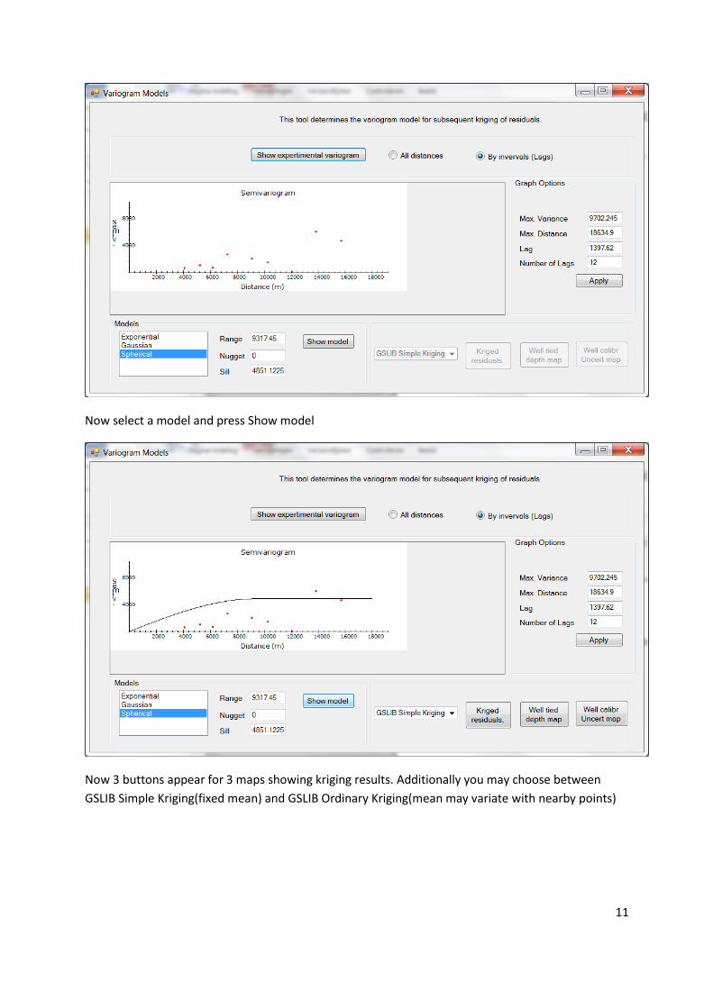
Now select a model and press Show model

Now 3 buttons appear for 3 maps showing kriging results. Additionally you may choose between

GSLIB Simple Kriging(fixed mean) and GSLIB Ordinary Kriging(mean may variate with nearby points)

12

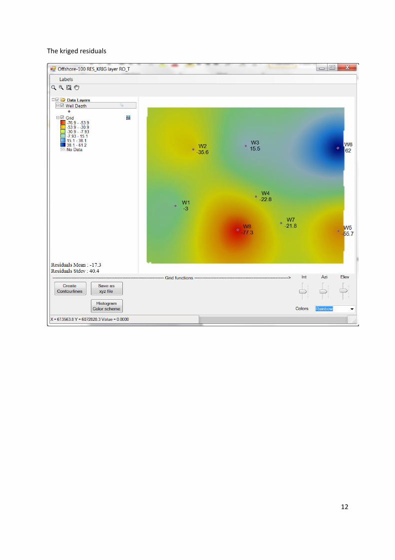
The kriged residuals

13

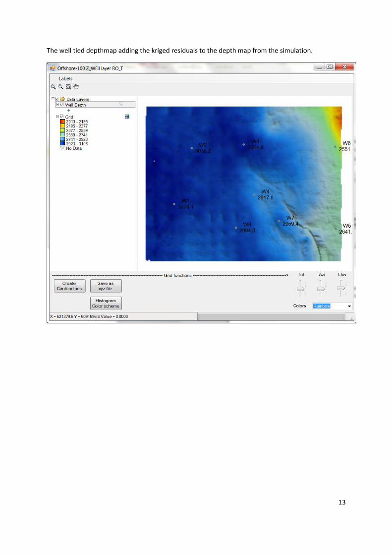
The well tied depthmap adding the kriged residuals to the depth map from the simulation.

14

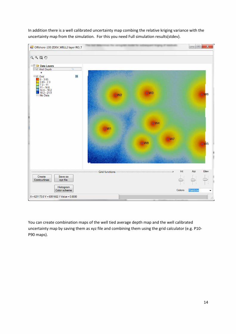
In addition there is a well calibrated uncertainty map combing the relative kriging variance with the

uncertainty map from the simulation. For this you need Full simulation results(stdev).

You can create combination maps of the well tied average depth map and the well calibrated

uncertainty map by saving them as xyz file and combining them using the grid calculator (e.g. P10-

P90 maps).

15

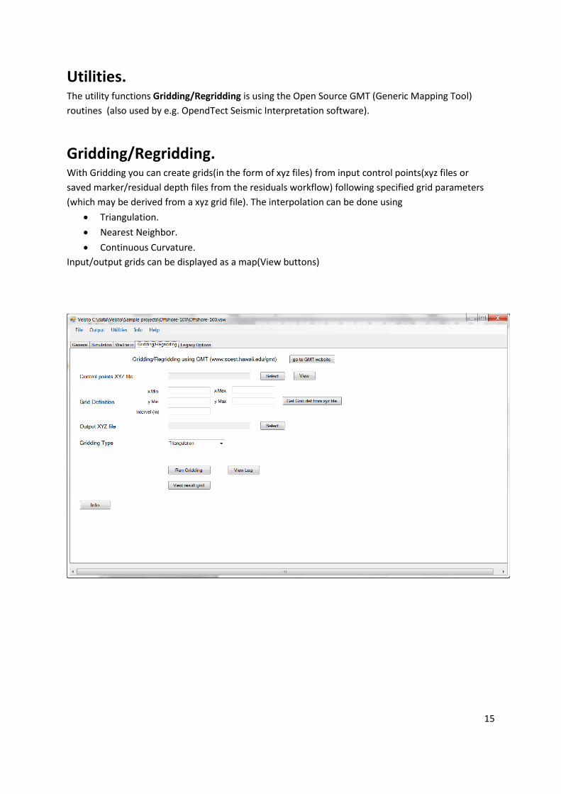
Utilities. The utility functions Gridding/Regridding is using the Open Source GMT (Generic Mapping Tool)

routines (also used by e.g. OpendTect Seismic Interpretation software).

Gridding/Regridding. With Gridding you can create grids(in the form of xyz files) from input control points(xyz files or

saved marker/residual depth files from the residuals workflow) following specified grid parameters

(which may be derived from a xyz grid file). The interpolation can be done using

Triangulation.

Nearest Neighbor.

Continuous Curvature.

Input/output grids can be displayed as a map(View buttons)

16

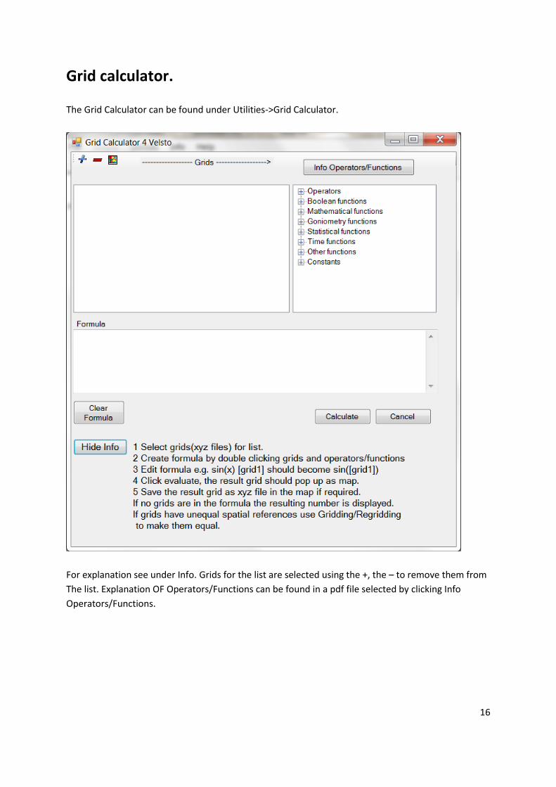
Grid calculator.

The Grid Calculator can be found under Utilities->Grid Calculator.

For explanation see under Info. Grids for the list are selected using the +, the – to remove them from

The list. Explanation OF Operators/Functions can be found in a pdf file selected by clicking Info

Operators/Functions.

17

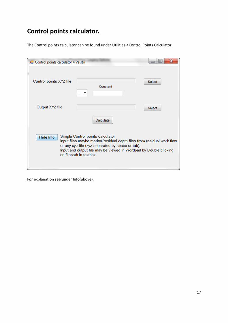
Control points calculator.

The Control points calculator can be found under Utilities->Control Points Calculator.

For explanation see under Info(above).

18

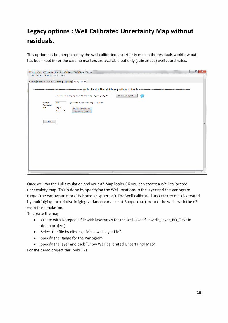
Legacy options : Well Calibrated Uncertainty Map without

residuals.

This option has been replaced by the well calibrated uncertainty map in the residuals workflow but

has been kept in for the case no markers are available but only (subsurface) well coordinates.

Once you ran the Full simulation and your σZ Map looks OK you can create a Well calibrated

uncertainty map. This is done by specifying the Well locations in the layer and the Variogram

range (the Variogram model is isotropic spherical). The Well calibrated uncertainty map is created

by multiplying the relative kriging variance(variance at Range = 1.0) around the wells with the σZ

from the simulation.

To create the map

Create with Notepad a file with layernr x y for the wells (see file wells_layer_RO_T.txt in

demo project)

Select the file by clicking “Select well layer file”.

Specify the Range for the Variogram.

Specify the layer and click “Show Well calibrated Uncertainty Map”.

For the demo project this looks like

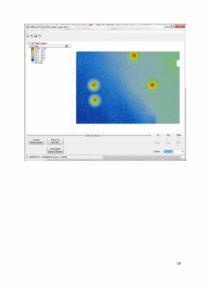
19