Velocity-Field Theory, Boltzmann's Transport …qft.web/2013/slides/...Velocity-Field Theory, Boltzmann’s Transport Equation, Geometry and Emergent Time Shoichi Ichinose [email protected]

.

.

. ..

.

.

Velocity-Field Theory, Boltzmann’s Transport

Equation, Geometry and Emergent Time

Shoichi Ichinose

[email protected]

Laboratory of Physics, SFNS, University of Shizuoka

「場の理論と弦理論」 YITP workshop , Kyoto, JapanArXiv:1303.6616(hep-th), Aug. 20, 2013

Shoichi Ichinose (Univ. of Shizuoka) Velocity-Field Theory, Boltzmann’s Transport Equation, Geometry and Emergent Time「場の理論と弦理論」 YITP workshop , Kyoto, Japan ArXiv:1303.6616(hep-th), Aug. 20, 2013 1

/ 36

[email protected]

1. Introduction

Sec 1. Introduction: a.Boltzmann eq.

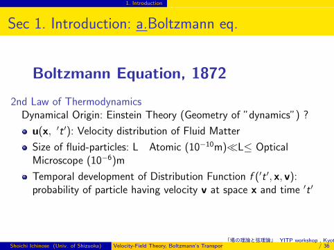
Boltzmann Equation, 1872

2nd Law of ThermodynamicsDynamical Origin: Einstein Theory (Geometry of ”dynamics”) ?

u(x, ′t ′): Velocity distribution of Fluid Matter

Size of fluid-particles: L Atomic (10−10m)≪L≤ OpticalMicroscope (10−6)m

Temporal development of Distribution Function f (′t ′, x, v):probability of particle having velocity v at space x and time ′t ′


/ 36

1. Introduction

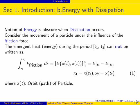
Sec 1. Introduction: b.Energy with Dissipation

Notion of Energy is obscure when Dissipation occurs.Consider the movement of a particle under the influence of thefriction force.The emergent heat (energy) during the period [t1, t2] can not bewritten as.∫ x2

x1

Ffriction dx = [E{x(t), x(t)}]t2t1 = E |t2 − E |t1 ,

x1 = x(t1), x2 = x(t2) (1)

where x(t): Orbit (path) of Particle.


/ 36

1. Introduction

Sec 1. Introduction: c.Discrete Morse Flow

Time should be re-considered, when dissipation occurs.→ Step-Wise approach to time-development.

Connection between step n and step n − 1 is determined by theminimal energy principle.

Time is ”emergent” from the principle.

Direction of flow (arrow of time) is built in from the beginning.

New approach to Statistical FluctuationDiscrete Morse Flow Method(Kikuchi, ’91)Holography (AdS/CFT, ’98)


/ 36

Sec 2. Emergent Time and Diffusion Equation

Sec 2. Emergent Time and Diff. Eq. a.Energy

Functional

1 dim viscous fluid, u(x): velocity field (distribution),Energy Functional

In[u(x)] =

∫dx

{σ

2ρ0(du

dx)2 + V (u) + u

dV 1(x)

dx+

1

2h(u − un−1)

2

}+ I 0n , σ ≡ 1, ρ0 ≡ 1, n = 1, 2, · · ·

V (u) =m2

2u2 +

λ

4!u4 , u = u(x) , un−1 = un−1(x) . (2)

periodic bound. cond. u(x) = u(x + 2l) , (3)


/ 36


Sec.2 Emer. T and Diff. Eq. : b.Variat. Principle

Variation δIn(u) = 0(u(x) → u(x) + δu(x)) gives Next step un(x)

1

h(un(x)− un−1(x)) =

σ

ρ0

d2undx2

− δV (un)

δun− dV 1

n (x)

dx, (4)

In[un] ≤ In[un−1] but In[un] ≤ In−1[un−1]does NOT hold . (5)

discrete time tn = nh = nτ0 × (h

τ0), τ0 ≡ h

√λσ/m, t0 ≡ 0. (6)

Noting u(x , tn) ≡ un(x), tn = tn−1 + h, as h → 0,

∂u(x , t)

∂t=

σ

ρ0

∂2u(x , t)

∂x2− δV (u(x , t))

δu(x , t)− ∂V 1(x , t)

∂x, 1 D diff. eq. (7)


/ 36


Sec.2 Emer. T and Diff. Eq. : b.Variat. Principle

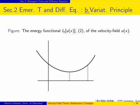
Figure: The energy functional In[u(x)], (2), of the velocity-field u(x).

In[u(x)]

un(x) un-1(x)

{u(x)}


/ 36


Sec.2 Emer T and Diff. Eq.: c.Burger’s Eq.

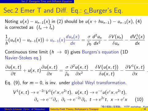
Noting u(x)− un−1(x) in (2) should be u(x + hun−1)− un−1(x), (4)is corrected as (In → In)

1

h(un(x)− un−1(x)) + un−1(x)

dun(x)

dx=

σ

ρ0

d2undx2

− δV (un)

δun− dV 1

n (x)

dx, (8)

Continuous time limit (h → 0) gives Burgers’s equation (1DNavier-Stokes eq.)

∂u(x , t)

∂t+ u(x , t)

∂u(x , t)

∂x=

σ

ρ0

∂2u(x , t)

∂x2− δV (u(x , t))

δu(x , t)− ∂V 1(x , t)

∂x. (9)

Eq. (9), for m = 0, is inv. under global Weyl transformation.

V 1(x , t) → e−2εV 1(eεx , e2εt), u(x , t) → e−εu(eεx , e2εt),

∂x → e−ε∂x , ∂t → e−2ε∂t , t → e2εt, x → eεx (10)


/ 36

Sec 3. Statistical Fluctuation Effect

Sec 3. Statistical Fluctuation Effect: a.Uncertainty

Large # of Particles→Statistical AverageInevitable uncertainty of Present Approach

1. The finite time-increment gives uncertainty to the minimal solutionun(x).2. The existence of the characteristic particle size gives uncertainty tothe minimal solution3. The system energy generally changes step by step.

Claim: the fluctuation comes not from the quantum effect butfrom the statistics caused by above points.


/ 36


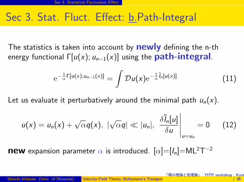
Sec 3. Stat. Fluct. Effect: b.Path-Integral

The statistics is taken into account by newly defining the n-thenergy functional Γ[u(x); un−1(x)] using the path-integral.

e−1αΓ[u(x);un−1(x)] =

∫Du(x)e−

1αIn[u(x)] (11)

Let us evaluate it perturbatively around the minimal path un(x).

u(x) = un(x) +√αq(x), |

√αq| ≪ |un|,

δIn[u]

δu

∣∣∣∣∣u=un

= 0 (12)

new expansion parameter α is introduced. [α]=[In]=ML2T−2


/ 36


Sec 3. Stat. Fluct. Effect: c.Not ~ But α

Claim: α should be small and should be chosen as

1) dimension is consistent

2) proportional to the small scale parameter whichcharacterizes the relevant physical phenomena (ex. themean-free path of the fluid particle). NOT includePlanck constant, ~, because fluctuation does not comefrom the quantum effect

3) the precise value should be best-fitted with theexperimental data


/ 36


Sec 3. Stat. Fluct. Effect: d.Background Field

The background-field method gives, at the Gaussian(quadratic,1-loop) approximation,

e−1αΓ[un(x);un−1(x)] = e−

1αIn[un(x)] × (detD)−1/2,

D ≡ − σ(= 1)

ρ0(= 1)

d2

dx2+ λun

2 +m2 +1

h− dun−1

dx,

(detD)−1/2 = exp

{1

2Tr

∫ ∞

0

e−τD

τdτ + const

}, (13)

([τ ]=[D−1]=L/M.)


/ 36


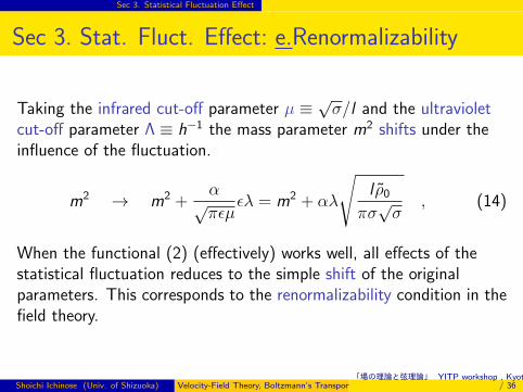
Sec 3. Stat. Fluct. Effect: e.Renormalizability

Taking the infrared cut-off parameter µ ≡√σ/l and the ultraviolet

cut-off parameter Λ ≡ h−1 the mass parameter m2 shifts under theinfluence of the fluctuation.

m2 → m2 +α

√πϵµ

ϵλ = m2 + αλ

√l ρ0

πσ√σ

, (14)

When the functional (2) (effectively) works well, all effects of thestatistical fluctuation reduces to the simple shift of the originalparameters. This corresponds to the renormalizability condition in thefield theory.


/ 36

Sec 4. Boltzmann’s Transport Equation

Sec 4. Boltzmann’s Transport Equation:

a.Step-Wise Approach

The step-wise development equation (8) with V 1n = 0, is written as

1

h(un(x)− un−1(x)) =

d2undx2

−m2un −λ

3!un

3 − un−1dundx

or un−1(x) =un(x)− h{d2un

dx2−m2un − λ

3!un

3}1− h dun

dx

. (15)

The equilibrium state u∞(x) , after sufficient recursive computation(n ≫ 1), satisfies

d2u∞

dx2−m2u∞ − λ

3!u∞3 − u∞du∞

dx= 0 , (16)


/ 36


Sec 4. Boltzmann’s Trans. Eq.: b.Distribution

The probability for the particle in the interval x ∼ x + dx andv ∼ v + dv , at the step n, is given by

1

Nn

fn(x , v)dxdv , fn(x , v): distribution function (17)

Then the n-th distribution fn(x , v) and the equilibrium distributionf ∞(x , v) can be introduced as

u∞(x) =1

ρ∞(x)

∫vf ∞(x , v)dv , un(x) =

1

ρn(x)

∫vfn(x , v)dv ,

un(x) → u∞(x) and fn(x , v) → f ∞(x , v) as n → ∞, (18)

where u∞(x) is the equilibrium velocity distribution. ρn(x) is theparticle number density. The continuity equation is given by

1

h(ρn(x)− ρn−1(x)) +

d

dx(ρn(x)un(x)) = 0 . (19)


/ 36


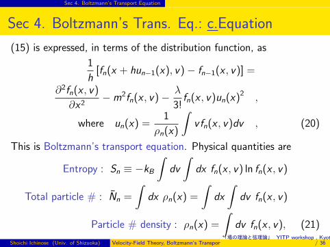
Sec 4. Boltzmann’s Trans. Eq.: c.Equation

(15) is expressed, in terms of the distribution function, as

1

h[fn(x + hun−1(x), v)− fn−1(x , v)] =

∂2fn(x , v)

∂x2−m2fn(x , v)−

λ

3!fn(x , v)un(x)

2 ,

where un(x) =1

ρn(x)

∫vfn(x , v)dv , (20)

This is Boltzmann’s transport equation. Physical quantities are

Entropy : Sn ≡ −kB

∫dv

∫dx fn(x , v) ln fn(x , v)

Total particle # : Nn =

∫dx ρn(x) =

∫dx

∫dv fn(x , v)

Particle # density : ρn(x) =

∫dv fn(x , v), (21)


/ 36


Sec 4. Boltzmann’s Trans. Eq.: d.Temperature

The momentum conservation at each point, x , requires

0 = ρn(x)

∫dv(v − un(x))fn(x , v), un(x) =

1

ρn(x)

∫dv v fn(x , v)(22)

Some distributions are given by

Temperature :1

2kBTn(x) ≡

1

ρn(x)

∫dv

m1

2(v − un(x))

2fn(x , v),

Heat Current : qn(x) ≡∫

dvm1

2(v − un(x))

3fn(x , v),

Pressure : Pn(x) ≡ m1

∫dv(v − un(x))

2fn(x , v), (23)


/ 36

Sec 5. Trajectory Geometry

Sec 5. Trajectory Geometry: a.Figure

Figure: The harmonic oscillator with friction.

-kx

-mg

Grav.Force

Fric.Force

Spring Forcex


/ 36


Sec 5. Traj. Geom.: b.Energy Funct. & Mini Princ.

The n-th energy function

Kn(x) = V (x) +η

2h(x − xn−1)

2 +m

2h2(x − 2xn−1 + xn−2)

2 + K 0n ,

Harmonic oscillator : V (x) = kx2/2, Constant : K 0n ,

friction coefficient : η, mass : m (24)

minimal principle : δKn = 0, x → x + δx .

Disc-Time Evol :δV

δx

∣∣∣∣x=xn

+η

h(xn − xn−1) +

m

h2(xn − 2xn−1 + xn−2) = 0

Diff Eq of HO with Friction :dV (x)

dx+ η

dx

dt+m

d2x

dt2= 0(25)

See Fig.2. This is a simple dissipative system.


/ 36


Sec 5. Traj. Geom.: c.Fluctuation from QM

Fluctuation of Path comes from uncertainty principle of quantummechanics in this case. ( 1 degree of freedom. No statisticalprocedure. )Classical value xn : x = xn +

√~ q where ~ is Planck constant.

e−1~hΓ(xn;xn−1,xn−2) =

∫dx e−

1~hKn(x) =

∫dq e−

1~hKn(xn+~q),

Γn ≡ Γ(xn; xn−1, xn−2) = Kn(xn) +~2h

ln(k +η

h+

m

h2) (26)

The quantum effect does not depend on the step number n.


/ 36


Sec 5. Traj. Geom.: d.Metric in Energy

xn − xn−1 ≡ ∆xn and (xn − 2xn−1 + xn−2)/h ≡ vn − vn−1 ≡ ∆vnWe find the metric in the energy at n-step.

Kn(xn) = V (xn) +η

2h(xn − xn−1)

2 +m

2h2(xn − 2xn−1 + xn−2)

2 + K 0n

=1

h2{V (xn)(∆t)2 +

ηh

2(∆xn)

2 +mh2

2(∆vn)

2}+ K 0n ,(27)

(∆sn)2 ≡ 2h2Kn(xn) = 2V (xn

′/√

ηh)(∆t)2 + (∆xn′)2 + (∆v ′

n)2 ,

xn′ ≡

√ηhxn , vn

′ ≡√mh2vn ,(28)

V (xn′/√ηh) = (k ′/2)xn

′2, k ′ ≡ k/ηh.Energy line-element ∆s2 in the (t, xn

′, vn′) space.

→ the geometrical basis for fixing the statistical ensemble.


/ 36


Sec 5. Traj. Geom.: e.Choice of K 0n

Taking the value K 0n as

K 0n = −V (xn)−

m

2h2(xn − 2xn−1 + xn−2)

2 + V (x0) +m

2h2(x1 − x0)

2,(29)

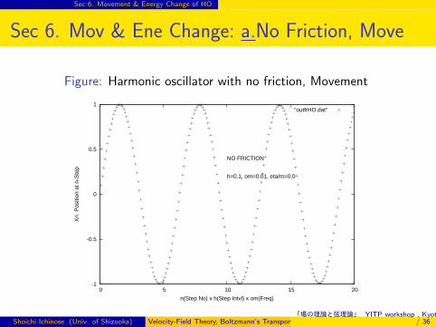
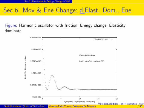
the graphs of movement and energy change, for various viscosities,are shown in Fig.3-9.no friction case: the oscillator keeps the initial energy (Fig.4).viscous case: the energy changes step by step, and finally reaches aconstant nonzero value (Fig.6,Fig.7, Fig.9).finally-remaining energy (constant) : dissipative one. Physically,the pressure and the temperature of the particle’s ”environment”.


/ 36

Sec 6. Movement & Energy Change of HO

Sec 6. Mov & Ene Change: a.No Friction, Move

Figure: Harmonic oscillator with no friction, Movement

-1

-0.5

0

0.5

1

0 5 10 15 20

Xn

Pos

ition

at n

-Ste

p

n(Step No) x h(Step Intvl) x om(Freq)

NO FRICTION

h=0.1, om=0.01, eta/m=0.0

"outfrHO.dat"


/ 36


Sec 6. Mov & Ene Change: b.No Friction, Energy

Figure: Harmonic oscillator with no friction, Energy change

9.9e-005

9.95e-005

0.0001

0.0001005

0.000101

0 5 10 15 20

Kn(

Xn)

/m E

nerg

y at

n-S

tep


NO FRICTION

h=0.1, om=0.01, eta/m=0.0

"EnefrHO.dat"


/ 36


Sec 6. Mov & Ene Change: c.Friction, Move

Figure: Harmonic oscillator with friction, Movement, (1)Elasticitydominate and (2)Viscosity dominate

-0.4

-0.2

0

0.2

0.4

0.6

0 5 10 15 20

Xn

Pos

ition

at n

-Ste

p


Viscosity Dominate

h=0.1, om=0.01, eta/m=0.03

Elasticity Dominate

h=0.1, om=0.01, eta/m=0.005

"outfrHO(2).dat""outFrHO(1).dat""outFrHO(1).dat"


/ 36


Sec 6. Mov & Ene Change: d.Elast. Dom., Ene

Figure: Harmonic oscillator with friction, Energy change, Elasticitydominate

9.37e-005

9.3705e-005

9.371e-005

9.3715e-005

9.372e-005

9.3725e-005

0 5 10 15 20

Kn(

Xn)

/m E

nerg

y at

n-S

tep


Elasticity Dominate

h=0.1, om=0.01, eta/m=0.005

"EnefrHO(1).dat"


/ 36


Sec 6. Mov & Ene Change: e.Visc. Dom., Ene

Figure: Harmonic oscillator with friction, Energy change, Viscositydominate

0.0001246

0.00012462

0.00012464

0.00012466

0.00012468

0.0001247

0.00012472

0.00012474

0 5 10 15 20

Kn(

Xn)

/m E

nerg

y at

n-S

tep


Viscosity Dominate

h=0.1, om=0.01, eta/m=0.03

"EnefrHO(2).dat"


/ 36


Sec 6. Mov & Ene Change: f.Reson, Move.

Figure: Harmonic oscillator with friction, Movement, Resonant

0

5

10

15

20

25

30

35

40

0 5 10 15 20

Xn

Pos

ition

at n

-Ste

p


RESONANT CASE

h=0.1, om=0.01, eta/m=0.02

"outfrHO(3).dat"


/ 36


Sec 6. Mov & Ene Change: g.Reson, Ene

Figure: Harmonic oscillator with friction, Energy change, Resonant

0.997

0.9975

0.998

0.9985

0.999

0 5 10 15 20

Kn(

Xn)

/m E

nerg

y at

n-S

tep


RESONANT CASE

h=0.1, om=0.01, eta/m=0.02

"EnefrHO(3).dat"


/ 36

Sec 7. Statistical Ensemble

Sec 7. Statistical Ensemble: a.Dirac-type Metric

Take N ’copies’ of previous model. Consider the ’macro’ system:N≫1. They interact each other and exchange energy, but we assumethe interaction is so moderate that every particle obeys the commonfield equation (25). They form a statistical ensemble caused by thearbitrariness of initial condition, Taking ”Dirac-type”metric[SI,2010Apr].

(ds2)D ≡ 2V (X )dt2 + dX 2 + dP2 − on-path →(2V (y) + y 2 + w 2)dt2,

LD =

∫ β

0

ds|on−path =

∫ β

0

√2V (y) + y 2 + w 2dt,

dµ = e−1αLDDyDw , e−βF =

∫ ∏n

dyndwne− 1

αLD , (30)

α: a parameter with dimension of length ([α]=L). See Fig.10.Shoichi Ichinose (Univ. of Shizuoka) Velocity-Field Theory, Boltzmann’s Transport Equation, Geometry and Emergent Time

「場の理論と弦理論」 YITP workshop , Kyoto, Japan ArXiv:1303.6616(hep-th), Aug. 20, 2013 30/ 36


Sec 7. Stat. Ensemble: b.Path(line) in 3D Bulk

Figure: The path of line in 3D bulk space (X,P,t).

t

X

0

P

(y(0),w(0))


/ 36


Sec 7. Stat. Ensemble: c.Standard Metric

Taking ”Standard-type” metric,

(ds2)S ≡ 1

dt2[(ds2)D ]

2 − on-path →

(2V (y) + y 2 + w 2)2dt2,

LS =

∫ β

0

ds|on−path =

∫ β

0

(2V (y) + y 2 + w 2)dt,

dµ = e−1αLSDyDw , e−βF =

∫ ∏n

dyndwne− 1

αLS . (31)

Exactly the same expression as the free energy expression in theFeynman’s textbook.


/ 36


Sec 7. Stat. Ensemble: d.Surfaces in 3D Bulk

Another choice: surfaces instead of lines.

X 2 + P2 = r 2(t) , 0 ≤ t ≤ β (32)

We respect here the isotropy of the 2 dim phase space (X ,P). SeeFig.11.


/ 36


Sec 7. Stat. Ensemble: e.Path(surface) in 3D Bulk

Figure: Two dimensional surface in 3D bulk space (X,P,t).

t

Xβ

0

(X=x(t),P=p(t))

P

r(t)

t


/ 36


Sec 7. Stat. Ensemble: f.Induced Metric & Area

induced metric gij on the surface (32)

(ds2)D∣∣on-path = 2V (X )dt2 + dX 2 + dP2

∣∣on-path

=2∑

i ,j=1

gijdXidX j , (gij) =

(1 + 2V

r2 r2X 2 2V

r2 r2XP

2Vr2 r2

PX 1 + 2Vr2 r2

P2

)(33)

where (X 1,X 2) = (X ,P). Area is given by

A =

∫ √det gijd

2X =

∫ √1 +

2V

r 2dXdP , (34)


/ 36


Sec 7. Stat. Ensemble: g.Path-Integral Measure

Consider all possible surfaces. Statistical distribution is

e−βF =

∫ ∞

0

dρ

∫r(0) = ρr(β) = ρ

∏t

DX (t)DP(t)e−1αA , (35)

We have directly defined the distribution function f (t, x , v) usinggeometry of the 3 dim bulk space.


/ 36

Documents

Velocity-Field Theory, Boltzmann's Transport …qft.web/2013/slides/...Velocity-Field Theory, Boltzmann’s Transport Equation, Geometry and Emergent Time Shoichi Ichinose [email protected]