Vehicle Testing and Data Analysis

Benjamin LabrosseBSc (Hons) Automotive Engineering

University of Wales Trinity Saint David

March 19, 2015

Lecturer: Tim Tudor

Contents

1. Introduction 81.1. Nomenclature . . . . . . . . . . . . . . . . . . . . . . . . . . . . . . . . . 9

2. Aerodynamic Principles 102.1. Drag . . . . . . . . . . . . . . . . . . . . . . . . . . . . . . . . . . . . . . 11

2.1.1. Drag calculation . . . . . . . . . . . . . . . . . . . . . . . . . . . 122.2. Longer path theory . . . . . . . . . . . . . . . . . . . . . . . . . . . . . . 13

2.2.1. Lift calculation . . . . . . . . . . . . . . . . . . . . . . . . . . . . 142.3. Balance . . . . . . . . . . . . . . . . . . . . . . . . . . . . . . . . . . . . 152.4. Testing methods of aerodynamics . . . . . . . . . . . . . . . . . . . . . . 16

3. Methodology 173.1. Simulator test process . . . . . . . . . . . . . . . . . . . . . . . . . . . . 173.2. Maths channels . . . . . . . . . . . . . . . . . . . . . . . . . . . . . . . . 18

4. Results and analysis 224.1. Coefficient of drag and rolling resistance . . . . . . . . . . . . . . . . . . 224.2. Coefficient of lift . . . . . . . . . . . . . . . . . . . . . . . . . . . . . . . 234.3. Lap analysis . . . . . . . . . . . . . . . . . . . . . . . . . . . . . . . . . . 25

4.3.1. Lift versus speed . . . . . . . . . . . . . . . . . . . . . . . . . . . 264.3.2. Lateral acceleration versus speed . . . . . . . . . . . . . . . . . . 264.3.3. Drag and lift . . . . . . . . . . . . . . . . . . . . . . . . . . . . . 294.3.4. Centre of pressure . . . . . . . . . . . . . . . . . . . . . . . . . . . 334.3.5. Understeer and oversteer . . . . . . . . . . . . . . . . . . . . . . . 35

5. Conclusion 385.1. Wing parameter selection . . . . . . . . . . . . . . . . . . . . . . . . . . 385.2. Further work . . . . . . . . . . . . . . . . . . . . . . . . . . . . . . . . . 38

Bibliography 38

2

A. Further research on aerodynamic principles 42A.1. Kutta Joukowski theorem . . . . . . . . . . . . . . . . . . . . . . . . . . 42A.2. Boundary layer and flow separation (skin friction) . . . . . . . . . . . . . 42

A.2.1. Boundary layer . . . . . . . . . . . . . . . . . . . . . . . . . . . . 42A.2.2. Flow separation . . . . . . . . . . . . . . . . . . . . . . . . . . . . 43

B. Simultaneous equations for drag calculation 45

3

List of Figures

2.0.1.Effect of increasing normal load on lateral tyre force, [Katz, 2006] . . . . 102.0.2.Effects on cornering acceleration due to aerodynamic devices, [Katz, 2006] 112.1.3.A typical velocity/time graph produced by a coast down test . . . . . . . 122.2.4.A diagram showing the method of creation of lift of wings, [Glenn Re-

search Center, 2014] . . . . . . . . . . . . . . . . . . . . . . . . . . . . . 132.2.5.A typical graph produced from a constant velocity test . . . . . . . . . . 14

4.1.1.The calculated coefficient of drag of the car . . . . . . . . . . . . . . . . . 234.1.2.Rolling resistance of the car depending on the AoA of both wings . . . . 244.2.3.Coefficient of lift of both wings dependent of the wing setup . . . . . . . 254.2.4.Graph showing the wing stall of the front wing when the front wing is

kept at a constant AoA . . . . . . . . . . . . . . . . . . . . . . . . . . . . 264.3.5.An x-y plot of lift versus velocity created in Pi Toolbox . . . . . . . . . . 274.3.6.A zoomed in section of the graph shown in Figure 4.3.5 . . . . . . . . . . 294.3.7.An x-y plot of lateral acceleration against speed . . . . . . . . . . . . . . 304.3.8.Screenshot showing the increased aero loads of setup F18R18 over F1R18

on the exit of Hatchet’s Hairpin . . . . . . . . . . . . . . . . . . . . . . . 314.3.9.A screenshot of drag and lift against distance, the top trace being drag

and bottom being lift . . . . . . . . . . . . . . . . . . . . . . . . . . . . . 324.3.10.Graph showing the driver lifting off the throttle (in the green box) between

Spitfires and Brooklands . . . . . . . . . . . . . . . . . . . . . . . . . . . 334.3.11.Graph showing the steering correction for setup F1R18 (red trace) . . . . 344.3.12.Plot showing the CoP of the car versus speed (bottom plot) and brake

and throttle position (top plot) . . . . . . . . . . . . . . . . . . . . . . . 354.3.13.Graph showing the theoretical and actual steering percentage for a lap . 36

A.2.1.Boundary layer of an airfoil that has been exagerrated for demonstrationpurposes, [John D. Anderson, 2005] . . . . . . . . . . . . . . . . . . . . . 43

4

A.2.2.Diagram showing the laminar and turbulent boundary layers, [de Haag,n,d] . . . . . . . . . . . . . . . . . . . . . . . . . . . . . . . . . . . . . . . 43

A.2.3.Graph depicting the change of pressure over an airfoil with an angle ofattack of 0°, [John D. Anderson, 2005] . . . . . . . . . . . . . . . . . . . 44

5

List of Tables

1.1.1.Table showing the definition of the nomenclature used within this report 9

3.1.1.The different wing parameters tested in the simulator sessions . . . . . . 173.1.2.The various ride height setups used to investigate effect of ride height on

aerodynamics . . . . . . . . . . . . . . . . . . . . . . . . . . . . . . . . . 183.1.3.The various rake parameters used in the simulator . . . . . . . . . . . . . 193.2.4.A list of the various maths channels created along with the corresponding

syntax . . . . . . . . . . . . . . . . . . . . . . . . . . . . . . . . . . . . . 203.2.5.A list of constants made in Pi . . . . . . . . . . . . . . . . . . . . . . . . 213.2.6.Table showing the different front and rear coefficients of lift for each setup 21

4.0.1.A table showing the driver feedback of each wing setup . . . . . . . . . . 224.3.2.A table showing the maximum and average speeds and maximum and

minimum lateral accelerations seen on track . . . . . . . . . . . . . . . . 284.3.3.Table comparing the theoretical steer percentage to the actual steer per-

centage on Hatchet’s hairpin . . . . . . . . . . . . . . . . . . . . . . . . . 364.3.4.Table comparing the theoretical steer percentage to the actual steer per-

centage on Honda . . . . . . . . . . . . . . . . . . . . . . . . . . . . . . . 37

5.1.1.Table showing the lap time for each wing setup . . . . . . . . . . . . . . 39

6

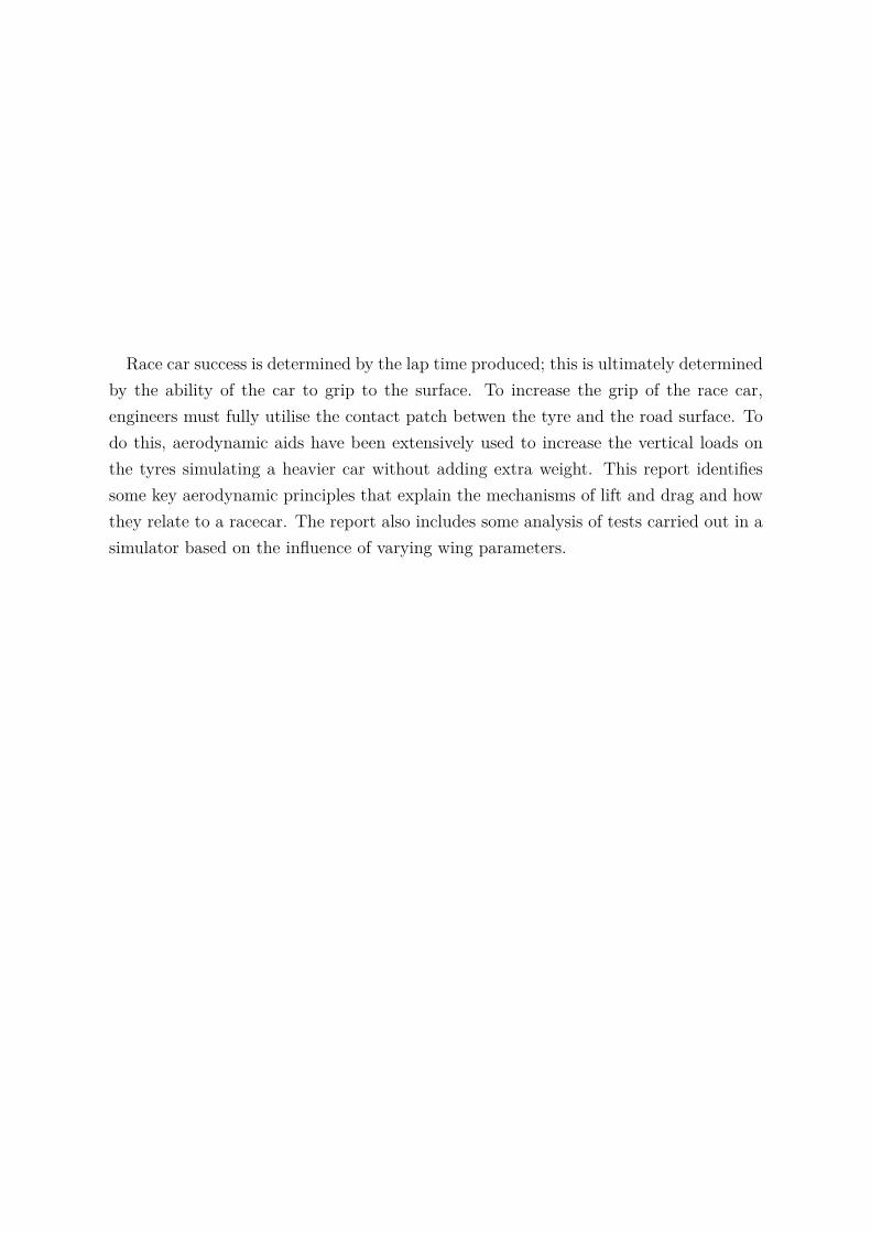
Race car success is determined by the lap time produced; this is ultimately determinedby the ability of the car to grip to the surface. To increase the grip of the race car,engineers must fully utilise the contact patch betwen the tyre and the road surface. Todo this, aerodynamic aids have been extensively used to increase the vertical loads onthe tyres simulating a heavier car without adding extra weight. This report identifiessome key aerodynamic principles that explain the mechanisms of lift and drag and howthey relate to a racecar. The report also includes some analysis of tests carried out in asimulator based on the influence of varying wing parameters.

1. Introduction

The use of aerodynamic components can change the driving characteristic of vehicles,more important in the high performance sector. Aerodynamic demands vary throughoutthe race season depending on the track being raced, leading to an easily changeable setup being advantageous. If a race track is predominantly based on top speed and has fewcorners then a lower downforce wold be beneficial to a track that has many turns andno high speed sections. Having a good data acquisition engineer will allow a race teamto analyse data gathered from testing, be it track, wind tunnel or computational fluiddynamics (CFD) and modify the setup accordingly.This leads to the aim of this report. It is the aim of the author to effectively analyse

the data obtained from a series of sessions in the Base Performance Simulator. Thisdata will be used to analyse the effect that changing the angle of attack of both frontand rear wings has on the handling characteristic of the F3 race car being tested. A fulltest procedure must be made to fully investigate the various aerodynamic parametersavailable and directions for the driver written up.Through the completion of this aim, the author will learn the fundamentals of aero-

dynamics and will learn the effects that various set ups has on the handling behaviourof the car.

8

1.1. Nomenclature

Symbol Definition Symbol DefinitionL Lift CD Coefficient of dragρ Density of fluid CL Coefficient of liftV∞ Flow velocity q∞ Fluid dynamic pressureΓ Vortex strength S Wing planform areap Pressure h Elevationv Velocity D Dragg Gravity

Table 1.1.1.: Table showing the definition of the nomenclature used within this report

9

2. Aerodynamic Principles

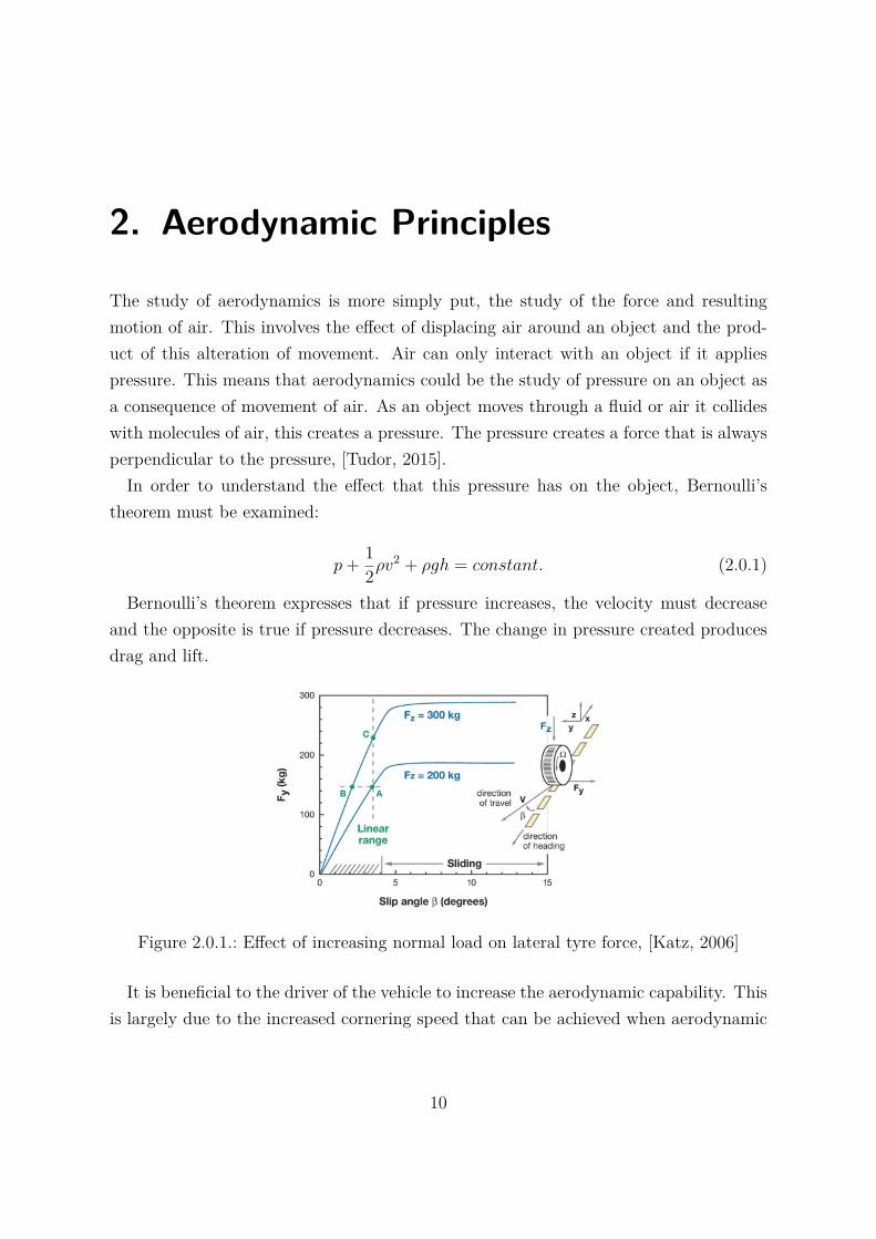
The study of aerodynamics is more simply put, the study of the force and resultingmotion of air. This involves the effect of displacing air around an object and the prod-uct of this alteration of movement. Air can only interact with an object if it appliespressure. This means that aerodynamics could be the study of pressure on an object asa consequence of movement of air. As an object moves through a fluid or air it collideswith molecules of air, this creates a pressure. The pressure creates a force that is alwaysperpendicular to the pressure, [Tudor, 2015].In order to understand the effect that this pressure has on the object, Bernoulli’s

theorem must be examined:

p+ 12ρv

2 + ρgh = constant. (2.0.1)

Bernoulli’s theorem expresses that if pressure increases, the velocity must decreaseand the opposite is true if pressure decreases. The change in pressure created producesdrag and lift.

Figure 2.0.1.: Effect of increasing normal load on lateral tyre force, [Katz, 2006]

It is beneficial to the driver of the vehicle to increase the aerodynamic capability. Thisis largely due to the increased cornering speed that can be achieved when aerodynamic

10

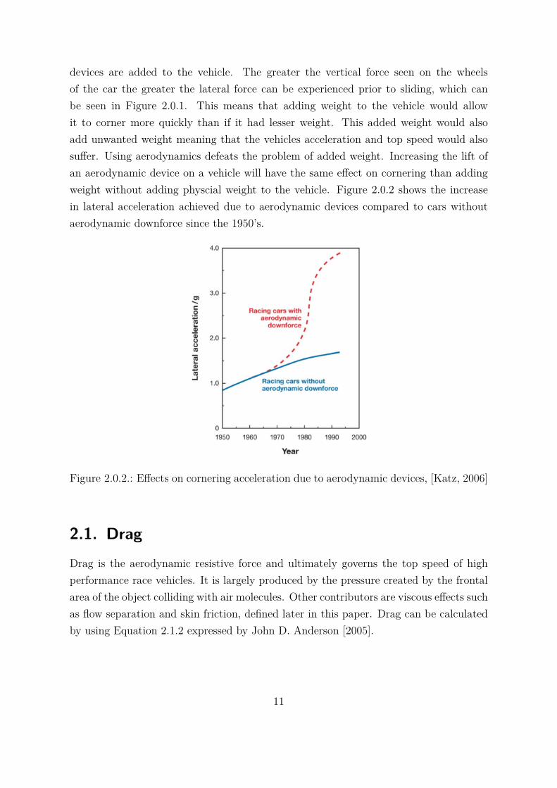
devices are added to the vehicle. The greater the vertical force seen on the wheelsof the car the greater the lateral force can be experienced prior to sliding, which canbe seen in Figure 2.0.1. This means that adding weight to the vehicle would allowit to corner more quickly than if it had lesser weight. This added weight would alsoadd unwanted weight meaning that the vehicles acceleration and top speed would alsosuffer. Using aerodynamics defeats the problem of added weight. Increasing the lift ofan aerodynamic device on a vehicle will have the same effect on cornering than addingweight without adding physcial weight to the vehicle. Figure 2.0.2 shows the increasein lateral acceleration achieved due to aerodynamic devices compared to cars withoutaerodynamic downforce since the 1950’s.

Figure 2.0.2.: Effects on cornering acceleration due to aerodynamic devices, [Katz, 2006]

2.1. DragDrag is the aerodynamic resistive force and ultimately governs the top speed of highperformance race vehicles. It is largely produced by the pressure created by the frontalarea of the object colliding with air molecules. Other contributors are viscous effects suchas flow separation and skin friction, defined later in this paper. Drag can be calculatedby using Equation 2.1.2 expressed by John D. Anderson [2005].

11

D = q∞SCD (2.1.2)

If any of these entities are not known, or if it is to be calculated through testing, themethod outlined in Section 2.1.1 can be used.

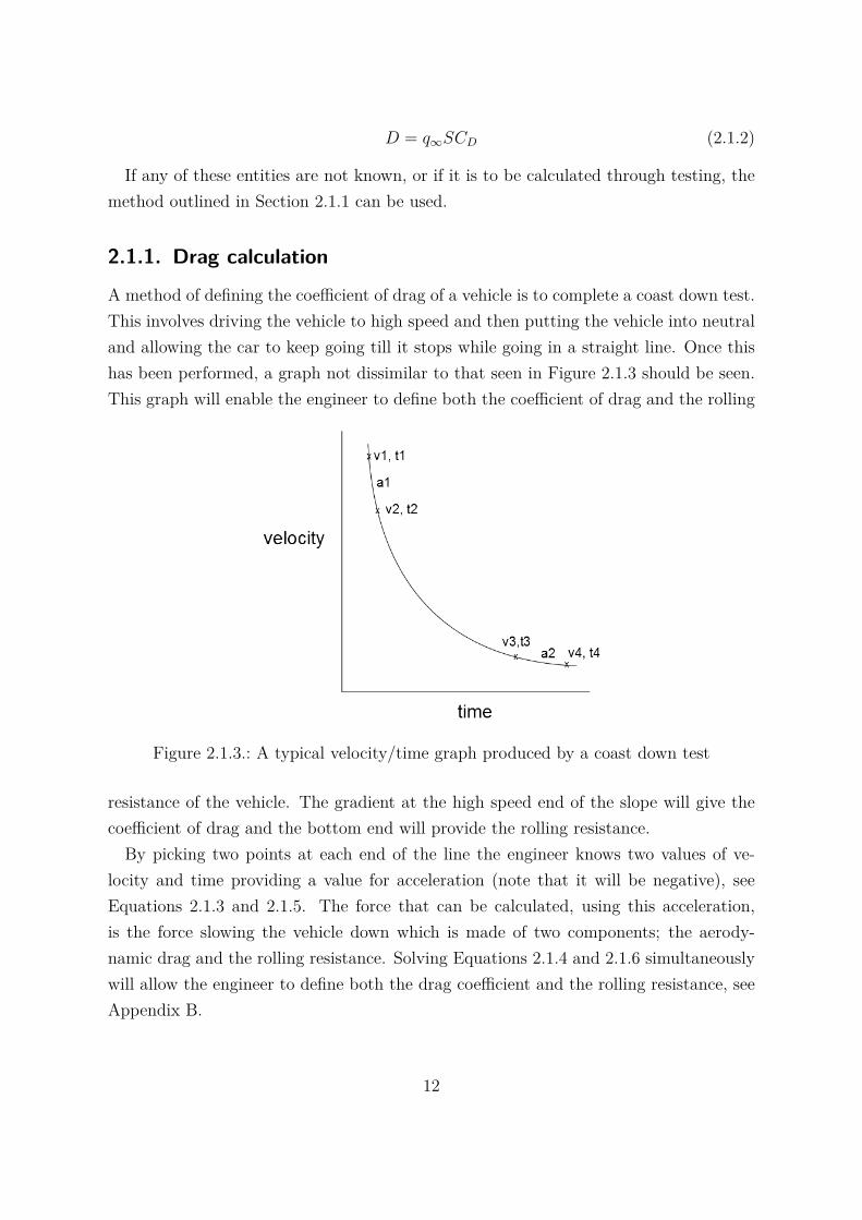
2.1.1. Drag calculation

A method of defining the coefficient of drag of a vehicle is to complete a coast down test.This involves driving the vehicle to high speed and then putting the vehicle into neutraland allowing the car to keep going till it stops while going in a straight line. Once thishas been performed, a graph not dissimilar to that seen in Figure 2.1.3 should be seen.This graph will enable the engineer to define both the coefficient of drag and the rolling

Figure 2.1.3.: A typical velocity/time graph produced by a coast down test

resistance of the vehicle. The gradient at the high speed end of the slope will give thecoefficient of drag and the bottom end will provide the rolling resistance.By picking two points at each end of the line the engineer knows two values of ve-

locity and time providing a value for acceleration (note that it will be negative), seeEquations 2.1.3 and 2.1.5. The force that can be calculated, using this acceleration,is the force slowing the vehicle down which is made of two components; the aerody-namic drag and the rolling resistance. Solving Equations 2.1.4 and 2.1.6 simultaneouslywill allow the engineer to define both the drag coefficient and the rolling resistance, seeAppendix B.

12

a1 = ∆v∆t = v2 − v1

t2 − t1(2.1.3)

F1 = ma1 = m(v2 − v1

t2 − t1) = 1

2ρCdAv21 +RR (2.1.4)

a2 = ∆v∆t = v4 − v3

t4 − t3(2.1.5)

F2 = ma2 = m(v4 − v3

t4 − t3) = 1

2ρCdAv22 +RR (2.1.6)

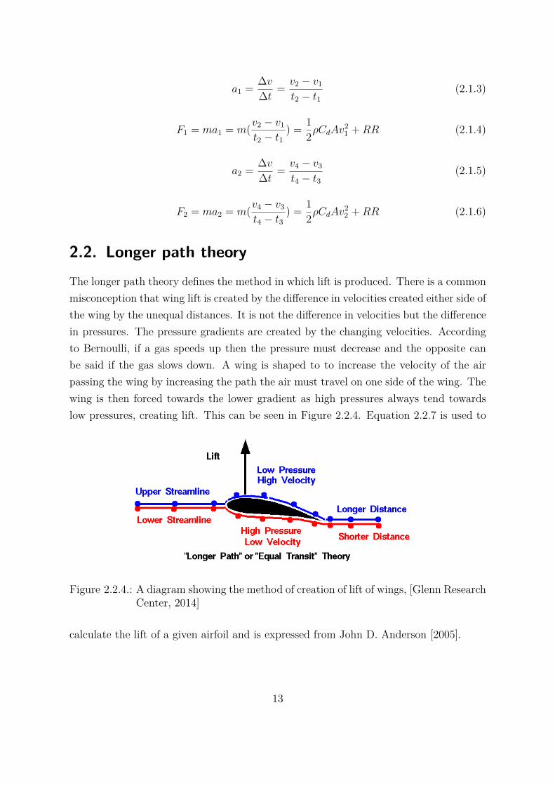
2.2. Longer path theoryThe longer path theory defines the method in which lift is produced. There is a commonmisconception that wing lift is created by the difference in velocities created either side ofthe wing by the unequal distances. It is not the difference in velocities but the differencein pressures. The pressure gradients are created by the changing velocities. Accordingto Bernoulli, if a gas speeds up then the pressure must decrease and the opposite canbe said if the gas slows down. A wing is shaped to to increase the velocity of the airpassing the wing by increasing the path the air must travel on one side of the wing. Thewing is then forced towards the lower gradient as high pressures always tend towardslow pressures, creating lift. This can be seen in Figure 2.2.4. Equation 2.2.7 is used to

Figure 2.2.4.: A diagram showing the method of creation of lift of wings, [Glenn ResearchCenter, 2014]

calculate the lift of a given airfoil and is expressed from John D. Anderson [2005].

13

L = q∞SCL (2.2.7)

2.2.1. Lift calculation

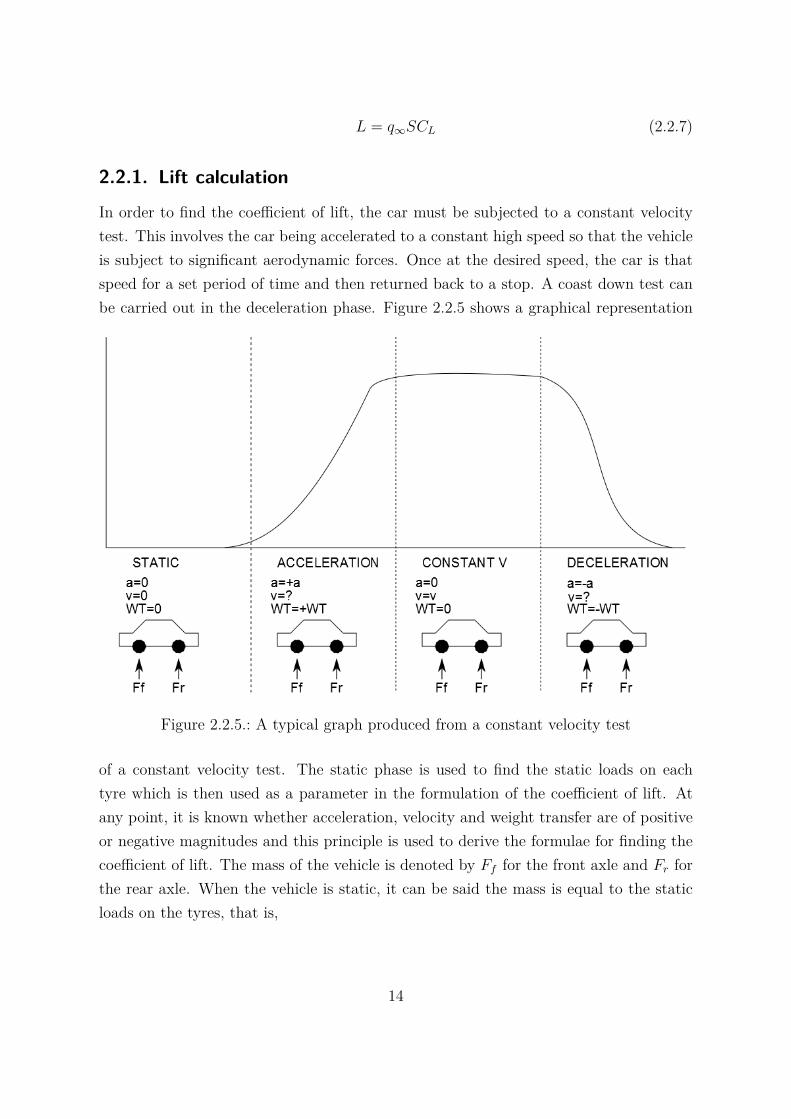
In order to find the coefficient of lift, the car must be subjected to a constant velocitytest. This involves the car being accelerated to a constant high speed so that the vehicleis subject to significant aerodynamic forces. Once at the desired speed, the car is thatspeed for a set period of time and then returned back to a stop. A coast down test canbe carried out in the deceleration phase. Figure 2.2.5 shows a graphical representation

Figure 2.2.5.: A typical graph produced from a constant velocity test

of a constant velocity test. The static phase is used to find the static loads on eachtyre which is then used as a parameter in the formulation of the coefficient of lift. Atany point, it is known whether acceleration, velocity and weight transfer are of positiveor negative magnitudes and this principle is used to derive the formulae for finding thecoefficient of lift. The mass of the vehicle is denoted by Ff for the front axle and Fr forthe rear axle. When the vehicle is static, it can be said the mass is equal to the staticloads on the tyres, that is,

14

Ff = Sf , (2.2.8)

Fr = Sr, (2.2.9)

where Sf and Sr denote the static loads of the front and rear axles respectively. Whenthe vehicle is in the acceleration phase it is subjected to aerodynamic forces and positiveweight transfer. This weight transfer will affect the aerodynamic properties due to thechanged angle of attack of the aerodynamic devices. This means the lift coefficient willdiffer to when the vehicle is at constant velocity. The force on the axles when acceleratingis therefore defined as:

Ff = Sf + 12ρCLfAv

2 −WT, (2.2.10)

Fr = Sr + 12ρCLrAv

2 +WT (2.2.11)

where CLf and CLr denotes the lift coefficient of the front and rear axles and WT isthe weight transfer. When the vehicle is in the constant velocity phase it is assumedthat only aerodynamic forces are affecting the forces on the axles with the forces beingdenoted by:

Ff = Sf + 12ρCLfAv

2, (2.2.12)

Fr = Sr + 12ρCLrAv

2. (2.2.13)

In order to define the lift coefficient these equations must be rewritten with the liftcoefficient as the subject of the equation.

2.3. BalanceIt is desirable for an engineer on a race team to know the balance of the race car andthe distribution of aerodynamic loads on the axles, that is, what percentage of theaerodynamic loads are acting on each axle. This will change how the car handles with abias to the front of the vehicle causing it to be less stable at high speeds but providinga greater initial turn in. A rear bias will make the car more stable at high speeds but

15

the car will tend to understeer. Driver feedback during the simulation tests will be usedto confirm these statements.In order to calculate the bias, the centre of pressure (CoP) must be found:

FAF = 12ρCLfAv

2 (2.3.14)

RAF = 12ρCLrAv

2 (2.3.15)

where FAF is the front aerodynamic force and RAF is the rear aerodynamic force. TheCoP is then found using Equation 2.3.16. This equation provides a percentage from thefront axle at which the centre of pressure acts on. This means that a number less than50 means there is a bias to the front axle and a number greater than 50 means the biastends towards the rear axle.

CoP = FAF

FAF +RAF× 100 (2.3.16)

2.4. Testing methods of aerodynamicsAccording to John Iley there are four main methods of testing for aerodynamics,

• Wind tunnel,

• Computational Fluid Dynamics (CFD),

• Track,

• Simulation,

stating that track testing is the most valuable method to use. He states that the otherthree forms of testing do not provide as accurate results as testing on a track, althoughsimulation has become relatively close to track testing.

16

3. Methodology

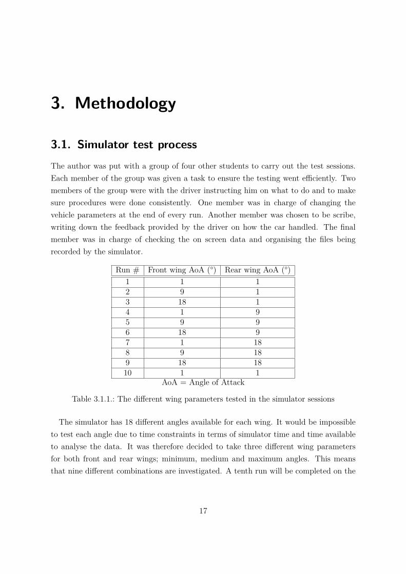
3.1. Simulator test processThe author was put with a group of four other students to carry out the test sessions.Each member of the group was given a task to ensure the testing went efficiently. Twomembers of the group were with the driver instructing him on what to do and to makesure procedures were done consistently. One member was in charge of changing thevehicle parameters at the end of every run. Another member was chosen to be scribe,writing down the feedback provided by the driver on how the car handled. The finalmember was in charge of checking the on screen data and organising the files beingrecorded by the simulator.

Run # Front wing AoA (°) Rear wing AoA (°)1 1 12 9 13 18 14 1 95 9 96 18 97 1 188 9 189 18 1810 1 1

AoA = Angle of Attack

Table 3.1.1.: The different wing parameters tested in the simulator sessions

The simulator has 18 different angles available for each wing. It would be impossibleto test each angle due to time constraints in terms of simulator time and time availableto analyse the data. It was therefore decided to take three different wing parametersfor both front and rear wings; minimum, medium and maximum angles. This meansthat nine different combinations are investigated. A tenth run will be completed on the

17

first parameter tested, this is to see how much quicker the driver completes the lap if atall and will allow the author to incorporate this difference into his analysis. The wingparameters being tested can be found in Table 3.1.1.

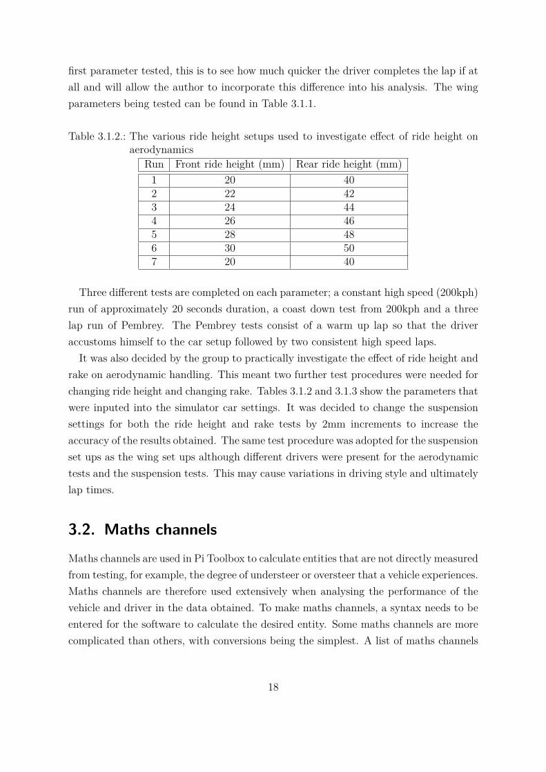
Table 3.1.2.: The various ride height setups used to investigate effect of ride height onaerodynamics

Run Front ride height (mm) Rear ride height (mm)1 20 402 22 423 24 444 26 465 28 486 30 507 20 40

Three different tests are completed on each parameter; a constant high speed (200kph)run of approximately 20 seconds duration, a coast down test from 200kph and a threelap run of Pembrey. The Pembrey tests consist of a warm up lap so that the driveraccustoms himself to the car setup followed by two consistent high speed laps.It was also decided by the group to practically investigate the effect of ride height and

rake on aerodynamic handling. This meant two further test procedures were needed forchanging ride height and changing rake. Tables 3.1.2 and 3.1.3 show the parameters thatwere inputed into the simulator car settings. It was decided to change the suspensionsettings for both the ride height and rake tests by 2mm increments to increase theaccuracy of the results obtained. The same test procedure was adopted for the suspensionset ups as the wing set ups although different drivers were present for the aerodynamictests and the suspension tests. This may cause variations in driving style and ultimatelylap times.

3.2. Maths channelsMaths channels are used in Pi Toolbox to calculate entities that are not directly measuredfrom testing, for example, the degree of understeer or oversteer that a vehicle experiences.Maths channels are therefore used extensively when analysing the performance of thevehicle and driver in the data obtained. To make maths channels, a syntax needs to beentered for the software to calculate the desired entity. Some maths channels are morecomplicated than others, with conversions being the simplest. A list of maths channels

18

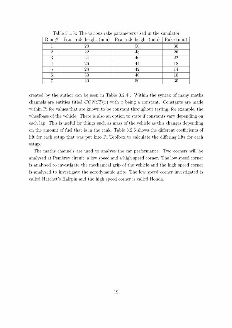
Table 3.1.3.: The various rake parameters used in the simulatorRun # Front ride height (mm) Rear ride height (mm) Rake (mm)

1 20 50 302 22 48 263 24 46 224 26 44 185 28 42 146 30 40 107 20 50 30

created by the author can be seen in Table 3.2.4 . Within the syntax of many mathschannels are entities titled CONST (x) with x being a constant. Constants are madewithin Pi for values that are known to be constant throughout testing, for example, thewheelbase of the vehicle. There is also an option to state if constants vary depending oneach lap. This is useful for things such as mass of the vehicle as this changes dependingon the amount of fuel that is in the tank. Table 3.2.6 shows the different coefficients oflift for each setup that was put into Pi Toolbox to calculate the differing lifts for eachsetup.The maths channels are used to analyse the car performance. Two corners will be

analysed at Pembrey circuit; a low speed and a high speed corner. The low speed corneris analysed to investigate the mechanical grip of the vehicle and the high speed corneris analysed to investigate the aerodynamic grip. The low speed corner investigated iscalled Hatchet’s Hairpin and the high speed corner is called Honda.

19

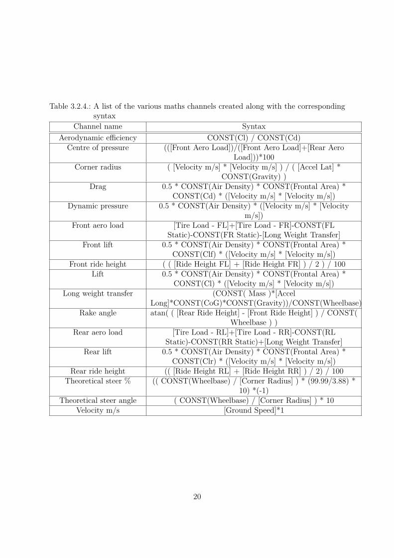
Table 3.2.4.: A list of the various maths channels created along with the correspondingsyntax

Channel name SyntaxAerodynamic efficiency CONST(Cl) / CONST(Cd)

Centre of pressure (([Front Aero Load])/([Front Aero Load]+[Rear AeroLoad]))*100

Corner radius ( [Velocity m/s] * [Velocity m/s] ) / ( [Accel Lat] *CONST(Gravity) )

Drag 0.5 * CONST(Air Density) * CONST(Frontal Area) *CONST(Cd) * ([Velocity m/s] * [Velocity m/s])

Dynamic pressure 0.5 * CONST(Air Density) * ([Velocity m/s] * [Velocitym/s])

Front aero load [Tire Load - FL]+[Tire Load - FR]-CONST(FLStatic)-CONST(FR Static)-[Long Weight Transfer]

Front lift 0.5 * CONST(Air Density) * CONST(Frontal Area) *CONST(Clf) * ([Velocity m/s] * [Velocity m/s])

Front ride height ( ( [Ride Height FL] + [Ride Height FR] ) / 2 ) / 100Lift 0.5 * CONST(Air Density) * CONST(Frontal Area) *

CONST(Cl) * ([Velocity m/s] * [Velocity m/s])Long weight transfer (CONST( Mass )*[Accel

Long]*CONST(CoG)*CONST(Gravity))/CONST(Wheelbase)Rake angle atan( ( [Rear Ride Height] - [Front Ride Height] ) / CONST(

Wheelbase ) )Rear aero load [Tire Load - RL]+[Tire Load - RR]-CONST(RL

Static)-CONST(RR Static)+[Long Weight Transfer]Rear lift 0.5 * CONST(Air Density) * CONST(Frontal Area) *

CONST(Clr) * ([Velocity m/s] * [Velocity m/s])Rear ride height (( [Ride Height RL] + [Ride Height RR] ) / 2) / 100

Theoretical steer % (( CONST(Wheelbase) / [Corner Radius] ) * (99.99/3.88) *10) *(-1)

Theoretical steer angle ( CONST(Wheelbase) / [Corner Radius] ) * 10Velocity m/s [Ground Speed]*1

20

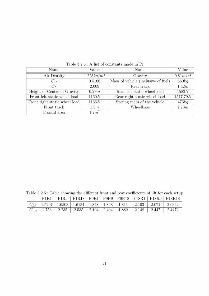
Table 3.2.5.: A list of constants made in PiName Value Name Value

Air Density 1.223kg/m3 Gravity 9.81m/s2

CD 0.5166 Mass of vehicle (inclusive of fuel) 560kgCL 2.009 Rear track 1.42m

Height of Centre of Gravity 0.23m Rear left static wheel load 1583NFront left static wheel load 1160N Rear right static wheel load 1577.79NFront right static wheel load 1166N Sprung mass of the vehicle 476kg

Front track 1.5m Wheelbase 2.73mFrontal area 1.2m2

Table 3.2.6.: Table showing the different front and rear coefficients of lift for each setupF1R1 F1R9 F1R18 F9R1 F9R9 F9R18 F18R1 F18R9 F18R18

CLF 1.5297 1.6503 1.6134 1.848 1.848 1.811 2.103 2.071 2.0342CLR 1.753 2.235 2.535 2.194 2.494 1.882 2.148 2.447 2.4472

21

4. Results and analysis

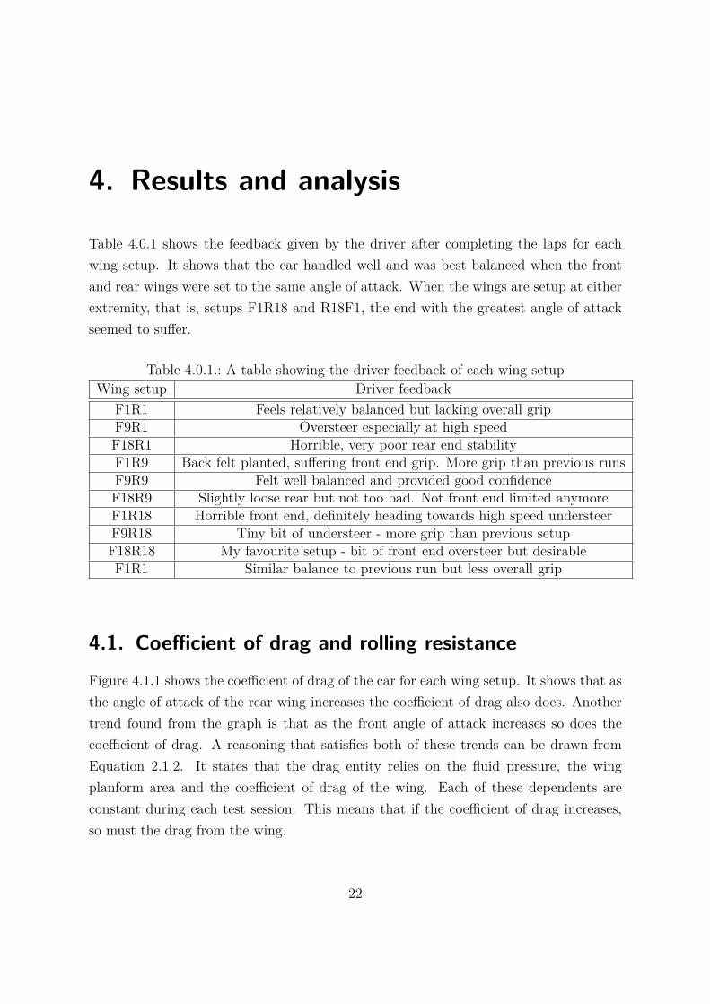
Table 4.0.1 shows the feedback given by the driver after completing the laps for eachwing setup. It shows that the car handled well and was best balanced when the frontand rear wings were set to the same angle of attack. When the wings are setup at eitherextremity, that is, setups F1R18 and R18F1, the end with the greatest angle of attackseemed to suffer.

Table 4.0.1.: A table showing the driver feedback of each wing setupWing setup Driver feedback

F1R1 Feels relatively balanced but lacking overall gripF9R1 Oversteer especially at high speedF18R1 Horrible, very poor rear end stabilityF1R9 Back felt planted, suffering front end grip. More grip than previous runsF9R9 Felt well balanced and provided good confidenceF18R9 Slightly loose rear but not too bad. Not front end limited anymoreF1R18 Horrible front end, definitely heading towards high speed understeerF9R18 Tiny bit of understeer - more grip than previous setupF18R18 My favourite setup - bit of front end oversteer but desirableF1R1 Similar balance to previous run but less overall grip

4.1. Coefficient of drag and rolling resistanceFigure 4.1.1 shows the coefficient of drag of the car for each wing setup. It shows that asthe angle of attack of the rear wing increases the coefficient of drag also does. Anothertrend found from the graph is that as the front angle of attack increases so does thecoefficient of drag. A reasoning that satisfies both of these trends can be drawn fromEquation 2.1.2. It states that the drag entity relies on the fluid pressure, the wingplanform area and the coefficient of drag of the wing. Each of these dependents areconstant during each test session. This means that if the coefficient of drag increases,so must the drag from the wing.

22

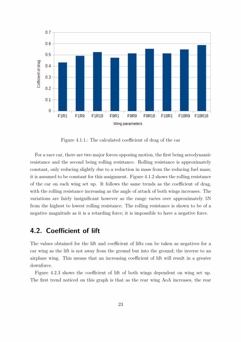
Figure 4.1.1.: The calculated coefficient of drag of the car

For a race car, there are two major forces opposing motion, the first being aerodynamicresistance and the second being rolling resistance. Rolling resistance is approximatelyconstant, only reducing slightly due to a reduction in mass from the reducing fuel mass;it is assumed to be constant for this assignment. Figure 4.1.2 shows the rolling resistanceof the car on each wing set up. It follows the same trends as the coefficient of drag,with the rolling resistance increasing as the angle of attack of both wings increases. Thevariations are fairly insignificant however as the range varies over approximately 5Nfrom the highest to lowest rolling resistance. The rolling resistance is shown to be of anegative magnitude as it is a retarding force; it is impossible to have a negative force.

4.2. Coefficient of liftThe values obtained for the lift and coefficient of lifts can be taken as negatives for acar wing as the lift is not away from the ground but into the ground; the inverse to anairplane wing. This means that an increasing coefficient of lift will result in a greaterdownforce.Figure 4.2.3 shows the coefficient of lift of both wings dependent on wing set up.

The first trend noticed on this graph is that as the rear wing AoA increases, the rear

23

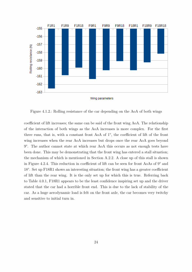
Figure 4.1.2.: Rolling resistance of the car depending on the AoA of both wings

coefficient of lift increases; the same can be said of the front wing AoA. The relationshipof the interaction of both wings as the AoA increases is more complex. For the firstthree runs, that is, with a constant front AoA of 1°, the coefficient of lift of the frontwing increases when the rear AoA increases but drops once the rear AoA goes beyond9°. The author cannot state at which rear AoA this occurs as not enough tests havebeen done. This may be demonstrating that the front wing has entered a stall situation;the mechanism of which is mentioned in Section A.2.2. A close up of this stall is shownin Figure 4.2.4. This reduction in coefficient of lift can be seen for front AoAs of 9° and18°. Set up F18R1 shows an interesting situation; the front wing has a greater coefficientof lift than the rear wing. It is the only set up for which this is true. Referring backto Table 4.0.1, F18R1 appears to be the least confidence inspiring set up and the driverstated that the car had a horrible front end. This is due to the lack of stability of thecar. As a huge aerodynamic load is felt on the front axle, the car becomes very twitchyand sensitive to initial turn in.

24

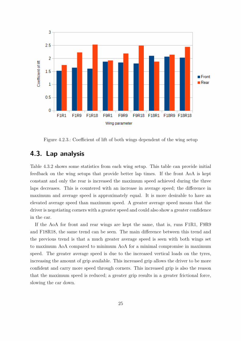
Figure 4.2.3.: Coefficient of lift of both wings dependent of the wing setup

4.3. Lap analysisTable 4.3.2 shows some statistics from each wing setup. This table can provide initialfeedback on the wing setups that provide better lap times. If the front AoA is keptconstant and only the rear is increased the maximum speed achieved during the threelaps decreases. This is countered with an increase in average speed; the difference inmaximum and average speed is approximately equal. It is more desirable to have anelevated average speed than maximum speed. A greater average speed means that thedriver is negotiating corners with a greater speed and could also show a greater confidencein the car.If the AoA for front and rear wings are kept the same, that is, runs F1R1, F9R9

and F18R18, the same trend can be seen. The main difference between this trend andthe previous trend is that a much greater average speed is seen with both wings setto maximum AoA compared to minimum AoA for a minimal compromise in maximumspeed. The greater average speed is due to the increased vertical loads on the tyres,increasing the amount of grip available. This increased grip allows the driver to be moreconfident and carry more speed through corners. This increased grip is also the reasonthat the maximum speed is reduced; a greater grip results in a greater frictional force,slowing the car down.

25

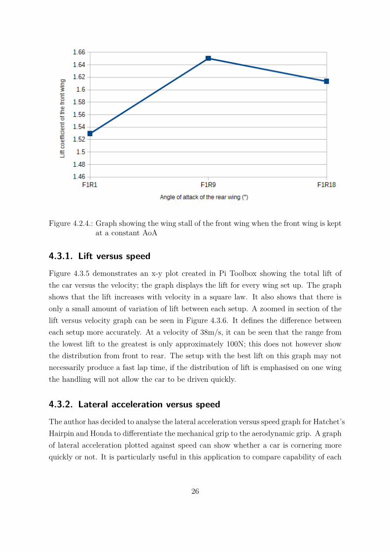
Figure 4.2.4.: Graph showing the wing stall of the front wing when the front wing is keptat a constant AoA

4.3.1. Lift versus speed

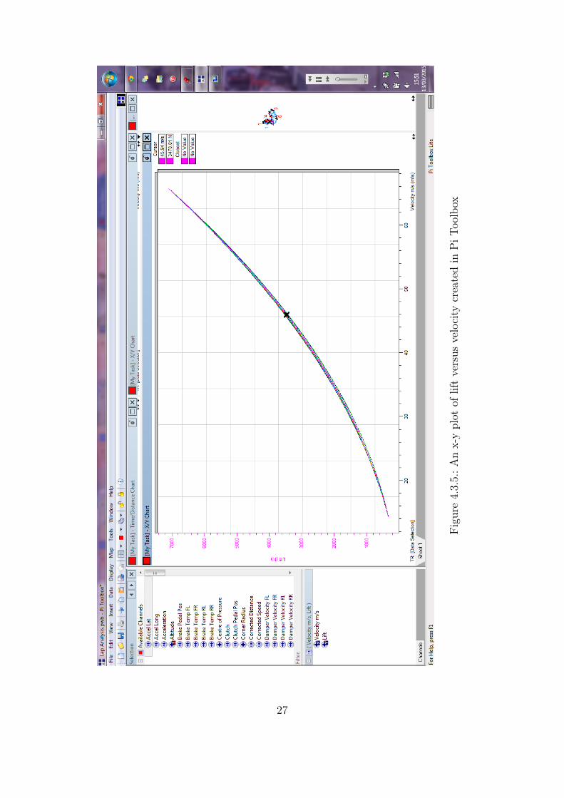
Figure 4.3.5 demonstrates an x-y plot created in Pi Toolbox showing the total lift ofthe car versus the velocity; the graph displays the lift for every wing set up. The graphshows that the lift increases with velocity in a square law. It also shows that there isonly a small amount of variation of lift between each setup. A zoomed in section of thelift versus velocity graph can be seen in Figure 4.3.6. It defines the difference betweeneach setup more accurately. At a velocity of 38m/s, it can be seen that the range fromthe lowest lift to the greatest is only approximately 100N; this does not however showthe distribution from front to rear. The setup with the best lift on this graph may notnecessarily produce a fast lap time, if the distribution of lift is emphasised on one wingthe handling will not allow the car to be driven quickly.

4.3.2. Lateral acceleration versus speed

The author has decided to analyse the lateral acceleration versus speed graph for Hatchet’sHairpin and Honda to differentiate the mechanical grip to the aerodynamic grip. A graphof lateral acceleration plotted against speed can show whether a car is cornering morequickly or not. It is particularly useful in this application to compare capability of each

26

Figu

re4.3.5.:A

nx-yplot

ofliftversus

velocity

createdin

PiTo

olbo

x

27

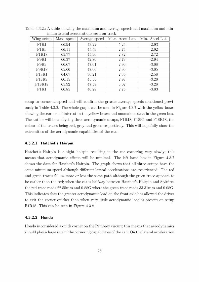
Table 4.3.2.: A table showing the maximum and average speeds and maximum and min-imum lateral accelerations seen on track

Wing setup Max. speed Average speed Max. Accel Lat. Min. Accel Lat.F1R1 66.94 43.22 5.24 -2.93F1R9 66.11 45.59 2.74 -2.92F1R18 65.77 45.96 2.82 -2.72F9R1 66.37 42.80 2.73 -2.94F9R9 66.67 47.01 2.96 -3.08F9R18 65.66 47.06 2.96 -3.05F18R1 64.67 36.21 2.36 -2.58F18R9 66.15 45.55 2.98 -3.20F18R18 65.92 47.58 3.02 -3.28F1R1 66.85 46.28 2.75 -3.03

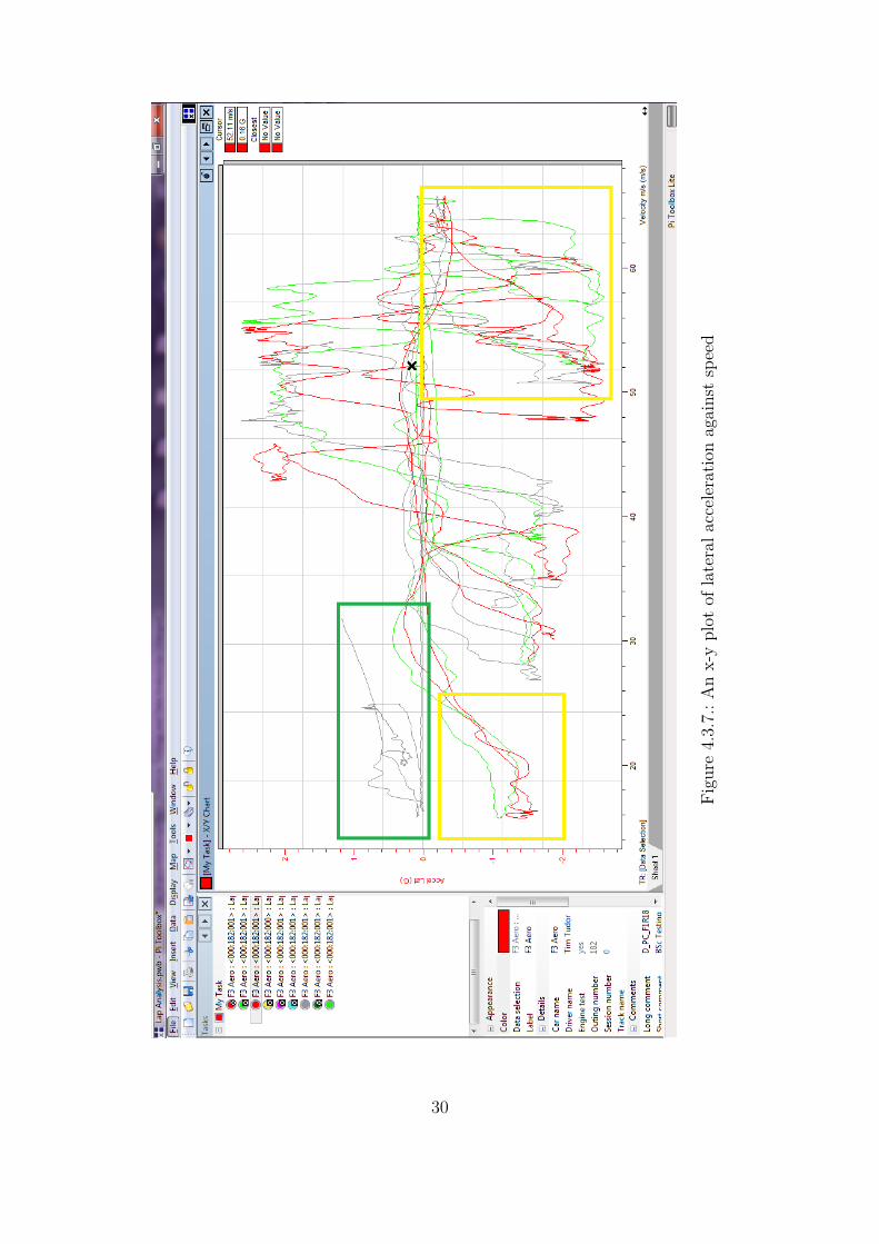
setup to corner at speed and will confirm the greater average speeds mentioned previ-ously in Table 4.3.2. The whole graph can be seen in Figure 4.3.7 with the yellow boxesshowing the corners of interest in the yellow boxes and anomalous data in the green box.The author will be analysing three aerodynamic setups, F1R18, F18R1 and F18R18, thecolour of the traces being red, grey and green respectively. This will hopefully show theextremities of the aerodynamic capabilities of the car.

4.3.2.1. Hatchet’s Hairpin

Hatchet’s Hairpin is a tight hairpin resulting in the car cornering very slowly; thismeans that aerodynamic effects will be minimal. The left hand box in Figure 4.3.7shows the data for Hatchet’s Hairpin. The graph shows that all three setups have thesame minimum speed although different lateral accelerations are experienced. The redand green traces follow more or less the same path although the green trace appears tobe earlier than the red; when the car is halfway between Hatchet’s Hairpin and Spitfiresthe red trace reads 22.55m/s and 0.88G where the green trace reads 33.31m/s and 0.08G.This indicates that the greater aerodynamic load on the front axle has allowed the driverto exit the corner quicker than when very little aerodynamic load is present on setupF1R18. This can be seen in Figure 4.3.8.

4.3.2.2. Honda

Honda is considered a quick corner on the Pembrey circuit; this means that aerodynamicsshould play a large role in the cornering capabilities of the car. On the lateral acceleration

28

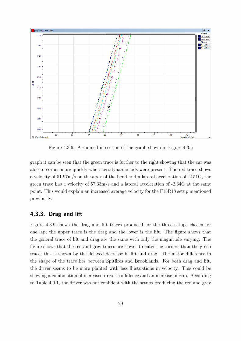
Figure 4.3.6.: A zoomed in section of the graph shown in Figure 4.3.5

graph it can be seen that the green trace is further to the right showing that the car wasable to corner more quickly when aerodynamic aids were present. The red trace showsa velocity of 51.97m/s on the apex of the bend and a lateral acceleration of -2.51G, thegreen trace has a velocity of 57.33m/s and a lateral acceleration of -2.34G at the samepoint. This would explain an increased average velocity for the F18R18 setup mentionedpreviously.

4.3.3. Drag and lift

Figure 4.3.9 shows the drag and lift traces produced for the three setups chosen forone lap; the upper trace is the drag and the lower is the lift. The figure shows thatthe general trace of lift and drag are the same with only the magnitude varying. Thefigure shows that the red and grey traces are slower to enter the corners than the greentrace; this is shown by the delayed decrease in lift and drag. The major difference inthe shape of the trace lies between Spitfires and Brooklands. For both drag and lift,the driver seems to be more planted with less fluctuations in velocity. This could beshowing a combination of increased driver confidence and an increase in grip. Accordingto Table 4.0.1, the driver was not confident with the setups producing the red and grey

29

Figu

re4.3.7.:A

nx-yplot

oflaterala

ccelerationagainstspeed

30

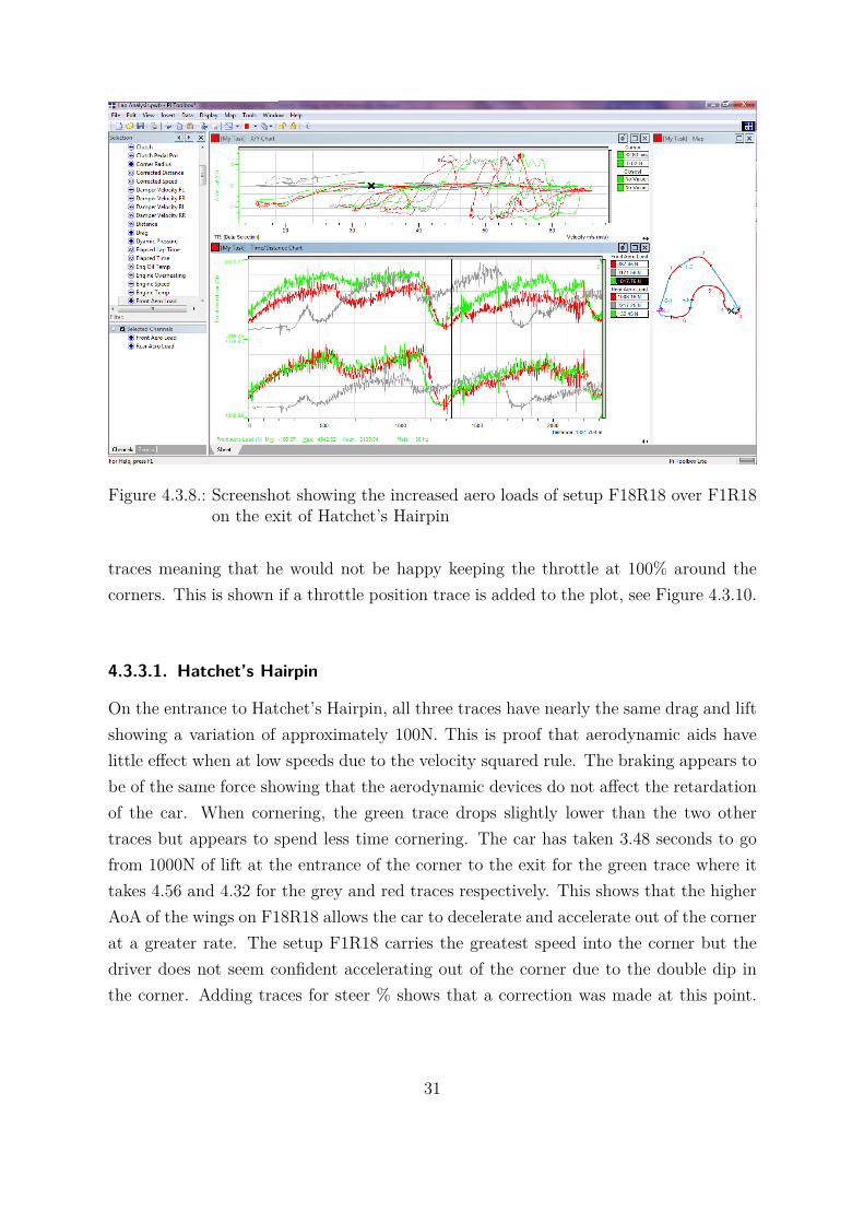
Figure 4.3.8.: Screenshot showing the increased aero loads of setup F18R18 over F1R18on the exit of Hatchet’s Hairpin

traces meaning that he would not be happy keeping the throttle at 100% around thecorners. This is shown if a throttle position trace is added to the plot, see Figure 4.3.10.

4.3.3.1. Hatchet’s Hairpin

On the entrance to Hatchet’s Hairpin, all three traces have nearly the same drag and liftshowing a variation of approximately 100N. This is proof that aerodynamic aids havelittle effect when at low speeds due to the velocity squared rule. The braking appears tobe of the same force showing that the aerodynamic devices do not affect the retardationof the car. When cornering, the green trace drops slightly lower than the two othertraces but appears to spend less time cornering. The car has taken 3.48 seconds to gofrom 1000N of lift at the entrance of the corner to the exit for the green trace where ittakes 4.56 and 4.32 for the grey and red traces respectively. This shows that the higherAoA of the wings on F18R18 allows the car to decelerate and accelerate out of the cornerat a greater rate. The setup F1R18 carries the greatest speed into the corner but thedriver does not seem confident accelerating out of the corner due to the double dip inthe corner. Adding traces for steer % shows that a correction was made at this point.

31

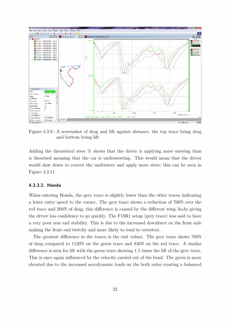
Figure 4.3.9.: A screenshot of drag and lift against distance, the top trace being dragand bottom being lift

Adding the theoretical steer % shows that the driver is applying more steering thanis theorised meaning that the car is understeering. This would mean that the driverwould slow down to correct the understeer and apply more steer; this can be seen inFigure 4.3.11.

4.3.3.2. Honda

When entering Honda, the grey trace is slightly lower than the other traces indicatinga lower entry speed to the corner. The grey trace shows a reduction of 700N over thered trace and 200N of drag; this difference is caused by the different wing AoAs givingthe driver less confidence to go quickly. The F18R1 setup (grey trace) was said to havea very poor rear end stability. This is due to the increased downforce on the front axlemaking the front end twitchy and more likely to tend to oversteer.The greatest difference in the traces is the exit values. The grey trace shows 780N

of drag compared to 1120N on the green trace and 830N on the red trace. A similardifference is seen for lift with the green trace showing 1.5 times the lift of the grey trace.This is once again influenced by the velocity carried out of the bend. The green is moreelevated due to the increased aerodynamic loads on the both axles creating a balanced

32

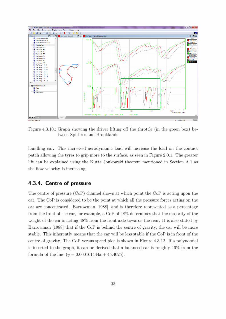
Figure 4.3.10.: Graph showing the driver lifting off the throttle (in the green box) be-tween Spitfires and Brooklands

handling car. This increased aerodynamic load will increase the load on the contactpatch allowing the tyres to grip more to the surface, as seen in Figure 2.0.1. The greaterlift can be explained using the Kutta Joukowski theorem mentioned in Section A.1 asthe flow velocity is increasing.

4.3.4. Centre of pressure

The centre of pressure (CoP) channel shows at which point the CoP is acting upon thecar. The CoP is considered to be the point at which all the pressure forces acting on thecar are concentrated, [Barrowman, 1988], and is therefore represented as a percentagefrom the front of the car, for example, a CoP of 48% determines that the majority of theweight of the car is acting 48% from the front axle towards the rear. It is also stated byBarrowman [1988] that if the CoP is behind the centre of gravity, the car will be morestable. This inherently means that the car will be less stable if the CoP is in front of thecentre of gravity. The CoP versus speed plot is shown in Figure 4.3.12. If a polynomialis inserted to the graph, it can be derived that a balanced car is roughly 46% from theformula of the line (y = 0.000161444x+ 45.4025).

33

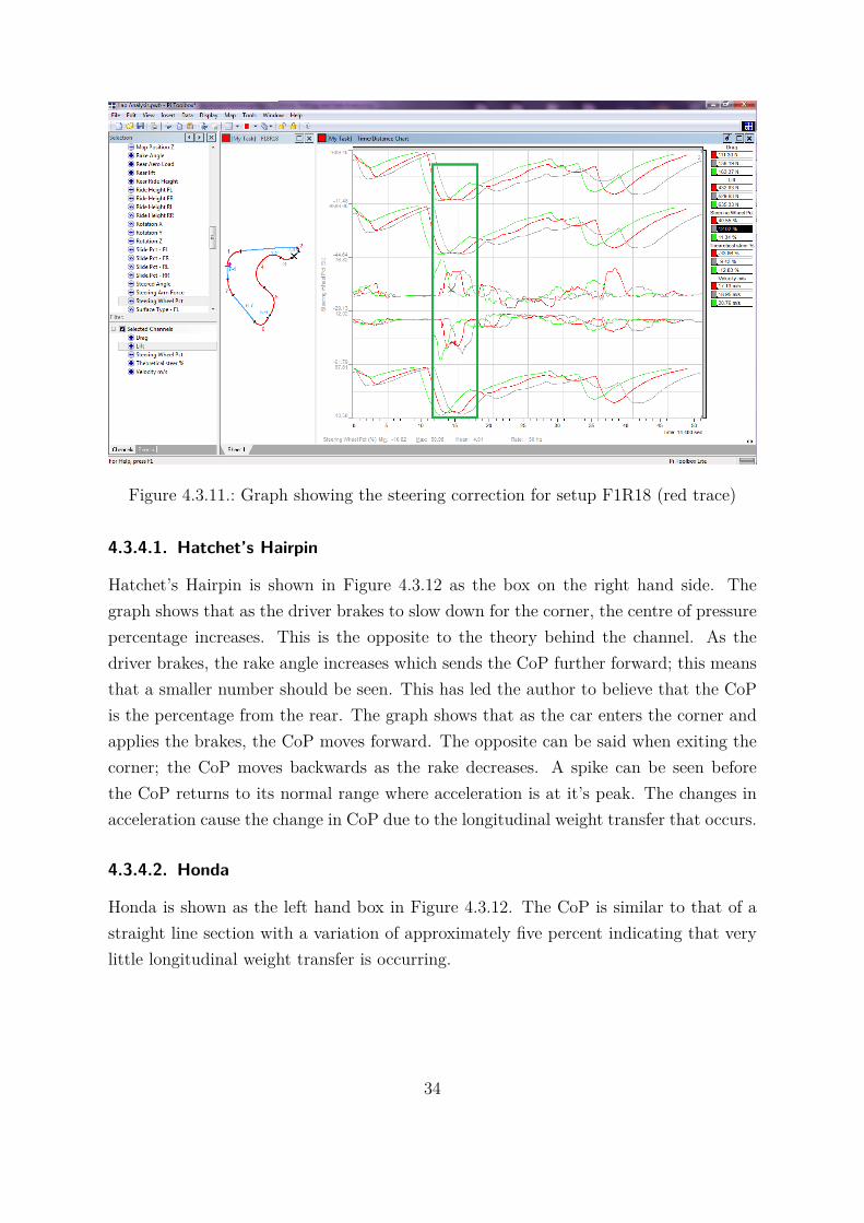
Figure 4.3.11.: Graph showing the steering correction for setup F1R18 (red trace)

4.3.4.1. Hatchet’s Hairpin

Hatchet’s Hairpin is shown in Figure 4.3.12 as the box on the right hand side. Thegraph shows that as the driver brakes to slow down for the corner, the centre of pressurepercentage increases. This is the opposite to the theory behind the channel. As thedriver brakes, the rake angle increases which sends the CoP further forward; this meansthat a smaller number should be seen. This has led the author to believe that the CoPis the percentage from the rear. The graph shows that as the car enters the corner andapplies the brakes, the CoP moves forward. The opposite can be said when exiting thecorner; the CoP moves backwards as the rake decreases. A spike can be seen beforethe CoP returns to its normal range where acceleration is at it’s peak. The changes inacceleration cause the change in CoP due to the longitudinal weight transfer that occurs.

4.3.4.2. Honda

Honda is shown as the left hand box in Figure 4.3.12. The CoP is similar to that of astraight line section with a variation of approximately five percent indicating that verylittle longitudinal weight transfer is occurring.

34

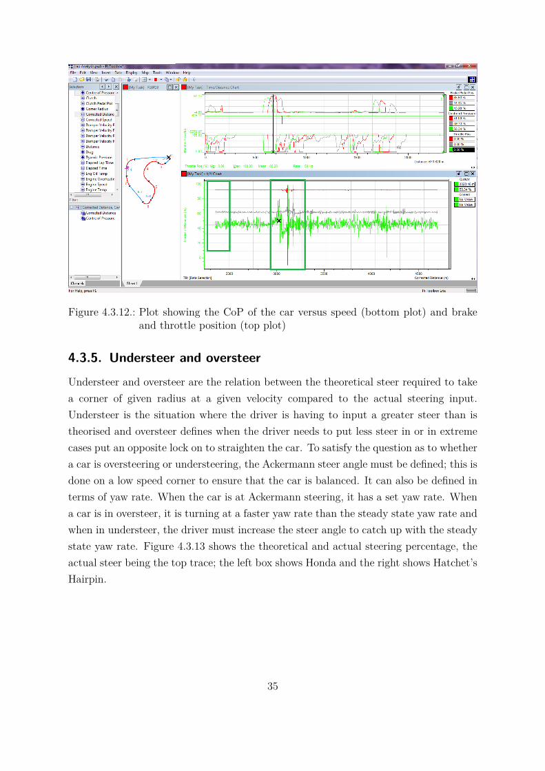
Figure 4.3.12.: Plot showing the CoP of the car versus speed (bottom plot) and brakeand throttle position (top plot)

4.3.5. Understeer and oversteer

Understeer and oversteer are the relation between the theoretical steer required to takea corner of given radius at a given velocity compared to the actual steering input.Understeer is the situation where the driver is having to input a greater steer than istheorised and oversteer defines when the driver needs to put less steer in or in extremecases put an opposite lock on to straighten the car. To satisfy the question as to whethera car is oversteering or understeering, the Ackermann steer angle must be defined; this isdone on a low speed corner to ensure that the car is balanced. It can also be defined interms of yaw rate. When the car is at Ackermann steering, it has a set yaw rate. Whena car is in oversteer, it is turning at a faster yaw rate than the steady state yaw rate andwhen in understeer, the driver must increase the steer angle to catch up with the steadystate yaw rate. Figure 4.3.13 shows the theoretical and actual steering percentage, theactual steer being the top trace; the left box shows Honda and the right shows Hatchet’sHairpin.

35

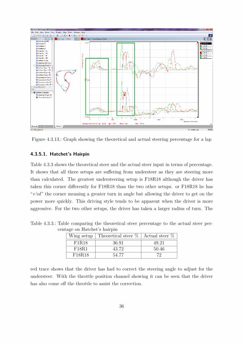
Figure 4.3.13.: Graph showing the theoretical and actual steering percentage for a lap

4.3.5.1. Hatchet’s Hairpin

Table 4.3.3 shows the theoretical steer and the actual steer input in terms of percentage.It shows that all three setups are suffering from understeer as they are steering morethan calculated. The greatest understeering setup is F18R18 although the driver hastaken this corner differently for F18R18 than the two other setups. or F18R18 he has“v’ed” the corner meaning a greater turn in angle but allowing the driver to get on thepower more quickly. This driving style tends to be apparent when the driver is moreaggressive. For the two other setups, the driver has taken a larger radius of turn. The

Table 4.3.3.: Table comparing the theoretical steer percentage to the actual steer per-centage on Hatchet’s hairpin

Wing setup Theoretical steer % Actual steer %F1R18 36.91 49.21F18R1 43.72 50.46F18R18 54.77 72

red trace shows that the driver has had to correct the steering angle to adjust for theundersteer. With the throttle position channel showing it can be seen that the driverhas also come off the throttle to assist the correction.

36

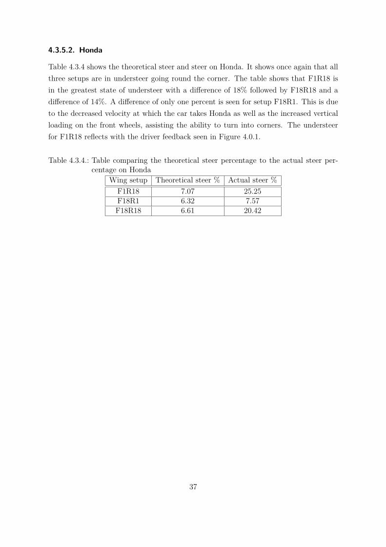
4.3.5.2. Honda

Table 4.3.4 shows the theoretical steer and steer on Honda. It shows once again that allthree setups are in understeer going round the corner. The table shows that F1R18 isin the greatest state of understeer with a difference of 18% followed by F18R18 and adifference of 14%. A difference of only one percent is seen for setup F18R1. This is dueto the decreased velocity at which the car takes Honda as well as the increased verticalloading on the front wheels, assisting the ability to turn into corners. The understeerfor F1R18 reflects with the driver feedback seen in Figure 4.0.1.

Table 4.3.4.: Table comparing the theoretical steer percentage to the actual steer per-centage on Honda

Wing setup Theoretical steer % Actual steer %F1R18 7.07 25.25F18R1 6.32 7.57F18R18 6.61 20.42

37

5. Conclusion

Due to time constraints the author was not able to fully analyse the setups that weretested; it was only feasible to analyse three out of the nine setups tested and only twocorners were analysed. This means that the conclusions brought together from the workin this assignment may not be entirely accurate as a setting that was not tested may bemore suitable.

5.1. Wing parameter selectionIt has been asked of the author to determine the most suited wing setup for a dry race.This can be identified by observing the differing aerodynamic capabilities of each wingsetup and deciding which setup has the best properties to produce a quick lap withminimal trade off in terms of drag. However, the author believes that the setup thatinspires the greatest confidence in the driver to push the car to the limits and producequick lap times would be the preferred setup for a race. The most aerodynamically soundsetup could be chosen but if the driver is not confident with the car then he will notproduce quick lap times. Table 5.1.1 shows the lap time for each wing setup. The setupthat produced the fastest time is F18R18 and according to Table 4.0.1 this setup provedto be the favourite setup of the driver. This leads the author to conclude that this isthe best setup to be used according to the data that was collected for this assignment.

5.2. Further workIf the author had a more designated time in the simulator he would have conductedmore tests investigating more setups; in particular finding the point at which the wingsenter a stall siuation. The author did not have the time to investigate the effect of rideheight and rake in the analysis although the methodology has been shown in this paperand the tests were conducted.

38

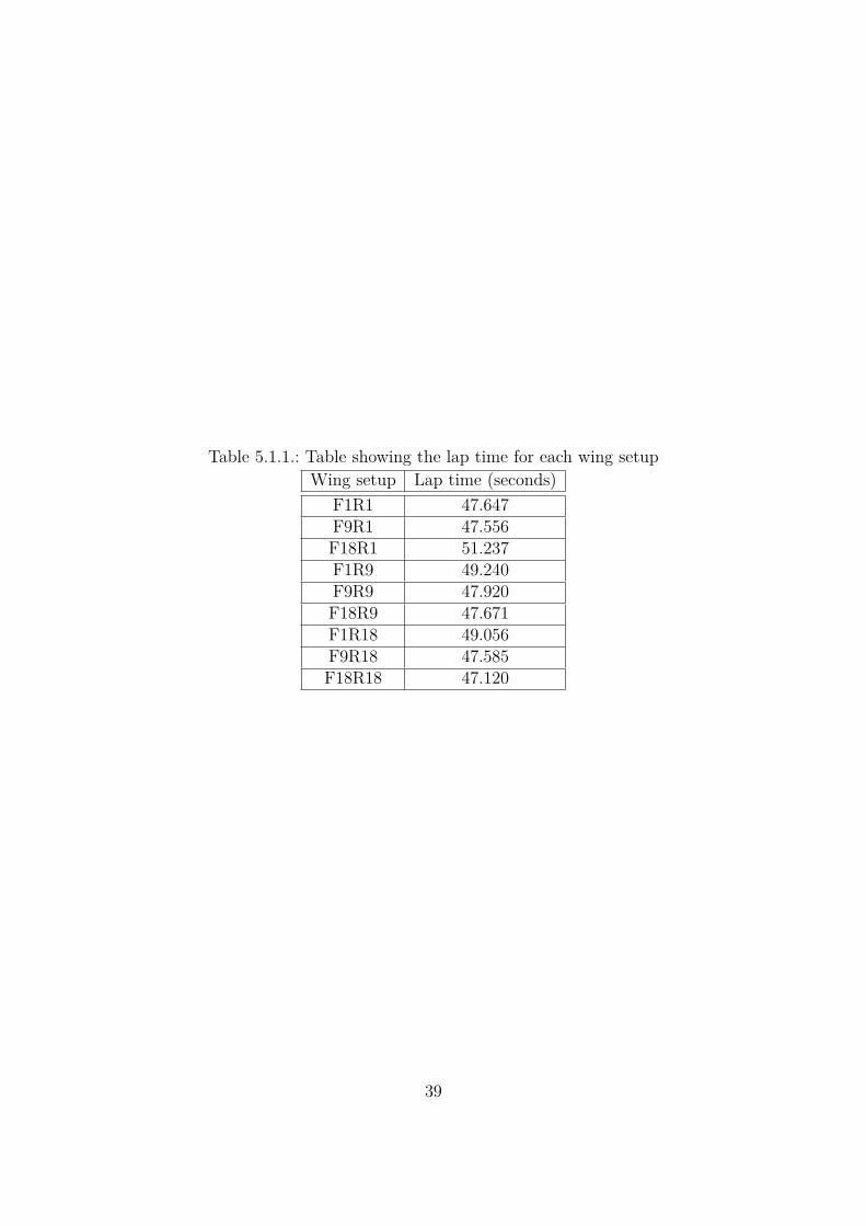
Table 5.1.1.: Table showing the lap time for each wing setupWing setup Lap time (seconds)

F1R1 47.647F9R1 47.556F18R1 51.237F1R9 49.240F9R9 47.920F18R9 47.671F1R18 49.056F9R18 47.585F18R18 47.120

39

Bibliography

Chenyuan Bai and ZIniu Wu. Generalized kutta-joukowski theorem for multi-vortexand multi-airfoil flow (a lumped vortex model). Technical report, School of Aerospace,Tsinghua University, Beijing, 2013. URL http://www.sciencedirect.com/science/article/pii/S1000936113001581.

James Barrowman. Calculating the center of pressure of a model rocket. Techni-cal report, Centuri Engineering Company, 1988. URL http://ftp.demec.ufpr.br/foguete/bibliografia/tir-33_CP.pdf.

Maarten Uijt de Haag. Basic aerodymamic principles and applications. Techni-cal report, Ohio University, n,d. URL http://www.ohio.edu/people/uijtdeha/chapter-2---basic-aerodynam.pdf.

Neha Ravi Dixit. Evaluation of vehicle understeer gradient definitions. Master’s thesis,The Ohio State University, 2009.

Glenn Research Center. Incorrect theory #1, 2014. URL http://www.grc.nasa.gov/WWW/k-12/airplane/wrong1.html. Editor: Tom Benson.

Jr. John D. Anderson. Introduction to Flight. McGraw-Hill Book Company, fifth edition,2005.

Joseph Katz. Aerodynamics of race cars. Annual Review of Fluid Mechanics, 38(1):27–63, 2006. doi: 10.1146/annurev.fluid.38.050304.092016. URL http://dx.doi.org/10.1146/annurev.fluid.38.050304.092016.

Aidan Lalor. Vehicle handling characteristics and development of a formula student car.Technical report, Swansea Metropolitan University, 2012.

Jorge Segers. Analysis Techniques for Racecar Data Acquisition. SAE International.,2014.

Tim Tudor. An introduction to aerodymamics. Lecture, 2015.

40

David H. Wood. Deriving the kutta-joukowsky equation and some of its generaliza-tions using momentum balances. Technical report, Department of Mechanical andManufacturing Engineering, Schulich School of Engineering, University of Calgary,2011.

41

A. Further research on aerodynamicprinciples

A.1. Kutta Joukowski theoremThe Kutta Joukowski theorem relates the circulation of air to the lift achieved by said aircirculation and can be seen in it’s analytical representation in Equation A.1.1, [de Haag,n,d].

L = −SV∞Γ (A.1.1)

The theorem assumes that the flow velocity acts upon an airfoil horizontally, that thedensity is constant and that a clockwise vortex has a negative sign, [Bai and Wu, 2013].At this point, drag is equal to zero.

A.2. Boundary layer and flow separation (skin friction)

A.2.1. Boundary layer

The boundary layer is a name for the retarded flow of air near the surface of an objectdue to friction between the gas and the surface of said object. This boundary layer can beseen in Figure A.2.1 where a represents the surface of the object at which point velocityis said to be zero and b is the outer edge where velocity is equal to the free flowing airflowing round the airfoil. The boundary layer thickness is denoted by δ and grows asthe flow of air progresses over the distance of the airfoil. Shear stress is experienced atthe surface of the airfoil due to the friction between the air and the airfoil surface andis denoted by τω. This shear stress contributes to aerodynamic drag in the form of skinfriction drag. The flow of air in the boundary layer is not uniform and is dependenton the Reynold’s number, smoothness of flow approaching the surface, the shape of theairfoil, the smoothness of the airfoil and the pressure gradient of the flow. The main

42

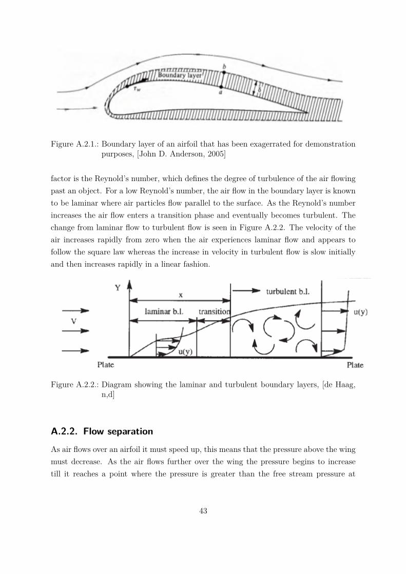
Figure A.2.1.: Boundary layer of an airfoil that has been exagerrated for demonstrationpurposes, [John D. Anderson, 2005]

factor is the Reynold’s number, which defines the degree of turbulence of the air flowingpast an object. For a low Reynold’s number, the air flow in the boundary layer is knownto be laminar where air particles flow parallel to the surface. As the Reynold’s numberincreases the air flow enters a transition phase and eventually becomes turbulent. Thechange from laminar flow to turbulent flow is seen in Figure A.2.2. The velocity of theair increases rapidly from zero when the air experiences laminar flow and appears tofollow the square law whereas the increase in velocity in turbulent flow is slow initiallyand then increases rapidly in a linear fashion.

Figure A.2.2.: Diagram showing the laminar and turbulent boundary layers, [de Haag,n,d]

A.2.2. Flow separation

As air flows over an airfoil it must speed up, this means that the pressure above the wingmust decrease. As the air flows further over the wing the pressure begins to increasetill it reaches a point where the pressure is greater than the free stream pressure at

43

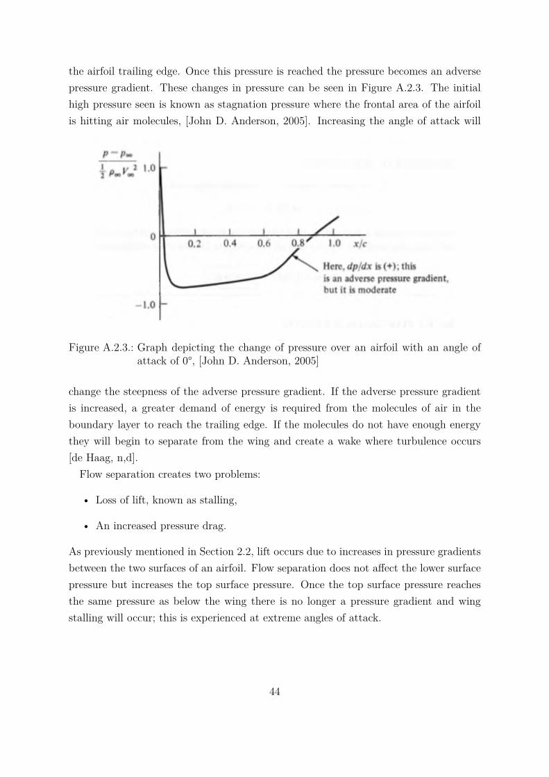
the airfoil trailing edge. Once this pressure is reached the pressure becomes an adversepressure gradient. These changes in pressure can be seen in Figure A.2.3. The initialhigh pressure seen is known as stagnation pressure where the frontal area of the airfoilis hitting air molecules, [John D. Anderson, 2005]. Increasing the angle of attack will

Figure A.2.3.: Graph depicting the change of pressure over an airfoil with an angle ofattack of 0°, [John D. Anderson, 2005]

change the steepness of the adverse pressure gradient. If the adverse pressure gradientis increased, a greater demand of energy is required from the molecules of air in theboundary layer to reach the trailing edge. If the molecules do not have enough energythey will begin to separate from the wing and create a wake where turbulence occurs[de Haag, n,d].Flow separation creates two problems:

• Loss of lift, known as stalling,

• An increased pressure drag.

As previously mentioned in Section 2.2, lift occurs due to increases in pressure gradientsbetween the two surfaces of an airfoil. Flow separation does not affect the lower surfacepressure but increases the top surface pressure. Once the top surface pressure reachesthe same pressure as below the wing there is no longer a pressure gradient and wingstalling will occur; this is experienced at extreme angles of attack.

44

B. Simultaneous equations for dragcalculation

Equations B.0.1 and B.0.2 are used as simultaneous equations to find CD and RR.

F1 = 12ρCDAv

21 +RR (B.0.1)

F2 = 12ρCDAv

22 +RR (B.0.2)

Equation B.0.1 is rearranged to solve for RR and can be seen in Equation B.0.3.

RR = F1 − 12ρCDAv

21 (B.0.3)

Equation B.0.3 is then substituted into Equation B.0.2 to make Equation B.0.4.

F2 = 12ρCDAv

22 + F1 − 1

2ρCDAv21 (B.0.4)

Equation B.0.4 is factorised to make Equation B.0.5.

F2 − F1 = 12ρACD(v2

2 − v21) (B.0.5)

Equation B.0.5 is rearranged to solve for CD and can be seen in Equation B.0.6.

CD = 2(F2 − F1)ρA(v2

2 − v21) (B.0.6)

Equation B.0.6 is substitued into Equation B.0.3 to make Equation B.0.7.

RR = F1 − 12ρ

2(F2 − F1)ρA(v2

2 − v21)Av

21 (B.0.7)

Equation B.0.7 is simplified to make Equation B.0.8.

45

RR = F1 − (F2 − F1)v21

v22 − v2

1(B.0.8)

46