Embed Size (px)
Citation preview

© ERIC 2007 www.eric.com.au 1
ERICERIC
VEGETATION: CONTINUUM OR DISCRETE STATES?
Brian Tunstall
Abstract
Environmental legislation treats vegetation similarly to species when they have very different
attributes. A key issue is whether vegetation forms discrete states, as with species, or a
continuum. This issue is addressed by way vegetation survey results for central Queensland,
central Sweden, and SW Queensland. The conservation implications of the conclusions are
discussed.
Introduction
Legislation on the conservation of biota initially addressed species and their environments.
Recent legislation greatly expands the entities provided protection, often identifying intent to
preserve. Vegetation is one such entity and it is treated similarly to species. It is assumed
there are distinct forms of vegetation and, given the desire for preservation, that these forms
are invariant over time. This attempt to preserve particular forms of vegetation has occurred
without consideration of whether distinct forms of vegetation exist, and whether existing
stands regarded as important can be preserved.
There is no logical basis for assigning attributes of species to the assemblages of species that
comprise vegetation. The genetic base of species restricts the nature and speed of evolutionary
change and this constraint does not arise with vegetation. Vegetation does not have the
attributes of species other than being composed of individuals that eventually die. Addressing
vegetation conservation requires addressing its characteristics rather than applying inapplicable
criteria developed for species.
This equating of species with vegetation is not explicit in legislation as traditional vegetation
descriptions usually identify discrete forms of plant communities. This has continued despite
the failure of numerous attempts to statistically demonstrate their existence. The forms of plant
communities identified using statistical analyses depend on how the vegetation was sampled
and the weightings used in analysis.
Landscape based approaches to vegetation mapping identify relationships between discrete
forms of plant communities and position in the landscape. While landscape related vegetation
patterns undoubtedly exist the reliability of extrapolation of results has not been properly
tested. The landscape approach to mapping has unknown reliability and, as with mapping of
discrete forms of vegetation, the results vary with the practitioner.
The notion of the existence of distinct forms of vegetation similarly to species is usually linked
with the successional theory of Clements (1916). While this theory has vegetation changing
over time through seral stages, it centres on the premise that vegetation develops to a
maximum (the climax) commensurate with the environment. Clements suggests there are
distinct forms of vegetation that reflect stable and maximal levels of vegetation development.
The Clementsian theory was widely adopted and applied because of its simplicity
and practicality. However, it was strongly questioned and commonly rejected by
those conducting research. The alternate individualistic concept (Gleason 1927) has ERICERIC
© ERIC 2007 www.eric.com.au 2
vegetation changing in response to the environment. While undisputedly correct this addresses
process but does not define outcomes. Theoretically a continuum of environment would
produce a continuum of vegetation but this was not demonstrated. The continuum concept
(McIntosh 1967, Whittaker 1975) explicitly suggests there should be an intergrade of
vegetation along an environmental gradient; a continuum of vegetation in response to a
continuum of environmental conditions.
Neither the theoretical considerations nor observations used in the development of the
concepts resolve the issue of whether vegetation occurs as a continuum or discrete states.
Even if vegetation does tend to a continuum there will be discrete states given disjuncts in the
environment. That is, there must be a continuum in environment to be able to observe a
continuum in vegetation. The difficulty lies in reliably identifying and characterising a
continuum in environment.
These issues were addressed by Tunstall (1987). They are further addressed here providing
new information on vegetation mapping and identifying general conservation implications.
The issue of preservation is not addressed as it is impossible to maintain a constant form of
vegetation. Even Clementsian theory invokes change through seral stages as temporal change
is inevitable with biology. Moreover, results by Walker et al. 1981 and Tunstall (2007)
demonstrate that vegetation does not remain at a stable maximum.
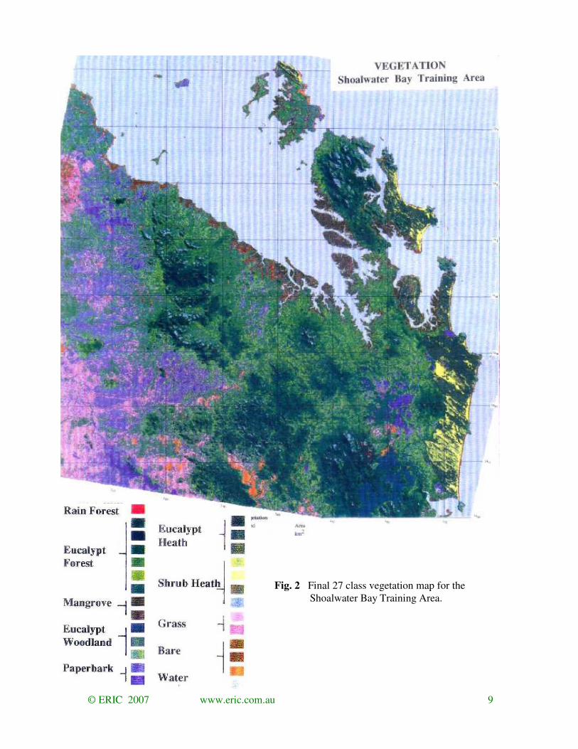
Vegetation Mapping SWBTA
Results from vegetation mapping in the Shoalwater Bay Training Area (SWBTA) in central
coastal Queensland are used to examine spatial relationships in largely undisturbed native
vegetation. The 2,700 km2 land area of SWBTA was heritage listed in the 1970s due to the
condition of the native vegetation. It was previously grazed, firstly by sheep and then cattle,
with 7% previously being cleared and around 50% selectively logged. Commercial grazing
was removed in 1964, forestry in 1972, and feral livestock around1990.
The vegetation is floristically complex with around 1000 vascular species. Most of the
vegetation is in good condition and much is pristine. However, the mapped area includes
some surrounding agricultural land much of which has been cleared and grazed by cattle.
The species diversity is associated with edaphic and climatic differences. The east west annual
rainfall gradient from 1750 to 800 mm is large. The broad environments include coastal
systems and western plains separated by a range. The coastal vegetation includes extensive
mangroves and sand dune systems. The western vegetation is typically paperbark and/or
eucalypt woodland.
Most soils are infertile but there are localised occurrences of reasonably fertile geologies.
Pockets of broad leafed (rainforest) vegetation exist in the ranges and on coastal plains.
Mapping method
The vegetation was mapped using numerical classification of a 1979 Landsat MSS image. The
procedure involved generating a large number of classes and iteratively grouping classes
taking account of spatial association and spectral similarity as well as class labels. Class labels
describe the vegetation associated with classes and were identified through field observation.
The mapping was checked using ground and aerial observations. Numerous low level
helicopter sorties were used to identify the form of vegetation in inaccessible locations, most
initiated for other purposes but some conducted specifically for vegetation survey. Ground

© ERIC 2007 www.eric.com.au 3
observations were accurately matched to the satellite mapping pre the availability of GPS and
georegistration of the image by transferring the satellite vegetation patterns to 1:25,000 colour
aerial photography.
The analysis spanned more than 5 years from 1981 and involved the development of the co-
occurrence statistic to incorporate spatial association in the analysis (Tunstall et al. 1984). The
co-occurrence analysis derives a normalised probability of a pixel in class i occurring
alongside one in class j. The i - i comparison indicates the cohesiveness of classes. The i - j
comparison indicates the level of spatial association between different classes. The statistic is
normalised to take account of the number of pixels in the classes.
The spatial associations between the 77 base classes across the entire mapped area identify that
all classes were spatially coherent (Fig.1). All classes are distinct. It also identifies that most
classes are only spatially associated (linked) with few other classes. Classes that are spectrally
similar tend to be spatially associated.
A final 27 class classification was produced by aggregating the base classes (Fig. 2). This
aggregation was zoned according to major environmental regions to eliminate the main
ambiguities. The base classification differentiated different forms of vegetation within general
environments such as hills, dry plains and wetlands but did not always discriminate between
distinct vegetation forms in the different environments. For example, mangroves in littoral
zone had the same spectral characteristics as Lysicarpus forest on the coastal plain and were
associated with the same base classes.
The zones used to stratify the base classification were sand dunes, coastal plain, marine plain,
ranges, and western plain. Different aggregations of classes were used for each zone.
Spatial associations on the western plains
Results for the western plains are used to illustrate the nature of spatial associations between
forms of vegetation. Most of the western plain is geologically reasonably uniform in being
derived from Pyri Pyri Granite. Old marine sediments occur at the south (Wandilla Formation
below Tilpal Creek). Recent sediments in the NW were associated with higher sea levels and
Herbert Creek draining the Fitzroy River. The localised volcanic Pine Mountain occurs in the
north
The spatial associations between the base and final classes are given in Fig. 3. The coloured
boxes identifying the final classes encompass aggregated base classes and so identify the
relationship between the base and final classifications.
The most open vegetation is grassland which links with paperbark woodland. In one direction
(down) the paperbark woodland links with wet paperbark communities. In the other direction
the sequence of vegetation is eucalypt / paperbark woodland, open eucalypt forest with
paperbark, and dense or open eucalypt forest (Fig 4). That is, regionally there is a sequence
from grassland through paperbark to eucalypt forest where paperbark is initially is dominant
and then forms an understory under eucalypts that decreases as the eucalypts increase.
While statistically discrete classes can be recognised, the results indicate that the vegetation
tends to form a continuum. For drained areas the sequence is from grassland through
increasing cover of paper bark to increasing cover of eucalypts, with the paperbarks decreasing
as the eucalypts increase.
The results identify spatial relationships that occur across a region of around 1,000 square
kilometres. The regional patterns relate to water supply by way of rainfall and drainage where

© ERIC 2007 www.eric.com.au 4
drainage is linked with fertility. Only a few localised patterns relate to the occurrence of more
fertile parent materials (geology / lithology). The patterns are landscape related but at a number
of scales.
The general floristic composition of the trees is 3 species of Melaleuca (nervosa, viridiflora,
leucodendra), 14 species in the Eucalyptus – Corymbia – Lophostemon complex (E
tereticornis, E alba, E exerta, E tracyhphloia, E populnea, E mollucana, E crebra, E
tessellaris, E papuana, C intermedia, C polycarpa, C dichromophloia, L suaveolens, L
conferta), Lysicarpus augustifolius and Allocasuarina leuhmanii. The number of species
allows for diverse combinations given the subtle variations in environments and wide overlap
in environmental limits for the species.
Some combinations of species effectively do not occur. While some omissions relate to
obvious environmental limits, as with eucalypts being intolerant to waterlogging, some are
without obvious explanation. For example, E populnea and E mollucana effectively do not
occur together despite occurring on similar soils in the same part of the landscape. Their
occurrence in SWBTA is lithology related, and E mollucana tends to be associated with C
citriodora on the hills and E populnea with E crebra. The only coexistence of E populnea and
E mollucana observed in central Queensland was a small patch on recent sediments in the
north west of the mapped area where E populnea was suppressed.
Conclusions SWBTA
The vegetation mapping involved the identification of discrete vegetation classes and was
needed to reduce the complexity to something that could be comprehended. While distinct
classes were identified the spatial associations indicate a continuous spatial progression
through classes. The results indicate that vegetation occurs as a continuum
An issue that arises with this conclusion is whether the result could derive from the analytical
method. The classification is broad, the imagery has a nominal 80m pixel (sample area of 60 x
80m), and the pixels are serially correlated. However, the appropriate pixel size for woody
vegetation is around 50m as the large size provides a reliable average. Also, while pixels are
serially correlated the aggregated pixels in classes are not.
While the pixel size may be appropriate the regular grid imposed by the satellite imager results
in some pixels being positioned on the overlap between vegetation forms. Pixels can be
composed of a number of vegetation forms (mixed pixels or mixels) and this introduces a
tendency to identify gradients rather than disjunct states. However, the classification identifies
the existence of classes where the spatial links between pixels within classes is much stronger
than between. The classes are statistically distinct.
While the classes are statistically distinct they are not homogeneous. The vegetation occurring
within a class includes forms that occur in spatially linked classes. That is, a sequence of
vegetation occurs within classes similarly to within the entire classification, as identified in
Fig.3. While the method may have a bias towards identifying gradients it cannot identify
gradients where they do not exist.
The broad classification does not include all vegetation forms that exist in the area. For
example, while Lysicarpus augustifolius (budgeroo) generally co-occurs with eucalypts and
paperbarks it can occur as monospecific stands. Within the study area this arose on a relict
beach ridge previously associated with Herbert Creek. However, as for the mix of eucalypts
and paperbarks, the composition of communities containing budgeroo comprises a continuum

© ERIC 2007 www.eric.com.au 5
from sparse individual to monospecific stands depending on the sandiness of the soil. There is
no apparent basis for identifying that the occurrence of a gradient derives from the method.
Vegetation patterns with simple floristics
Observations obtained in pine forests in central Sweden are reported in Tunstall and Torssell
(2004b). The climate, while severe, has little gradient and recent glaciation has produced
geologically and floristically simple systems. Most of the area is dominated by a single tree
species Pinus sylvestrus growing on sandy soils, with spruce (Picea abies) and birch (Betula
alba) being the only other tree species. Essentially only 6 understory ‘species’ occur under
pines, lichen, moss, and the shrubs Vaccinium myrtillus, Vaccinium vitis idaeus, Caluna
vulgaris, and Rubus idaeus
Sample sites were selected to encompass the full range of variation in vegetation. Results
identify that, while there are limits to what is observed, within those limits there is a full
spectrum of combinations (Fig 5). As the sampling was non-random the results cannot
identify any tendency for the preferential occurrence of particular forms of vegetation but they
do identify that all forms can occur.
The considerations of Clements centred on vegetation developing to a stable maximum
commensurate with the environment. The temporal development of pine illustrates that, while
there is a maximal level of development, it declines with time after it has been achieved. (Fig.
6). Moreover, the maximum is seldom achieved
While the coexisting species have distinct environmental preferences the vegetation does not
develop into distinct forms or states as the physical environment contains gradations. Also,
further gradations arise from the inevitable mortality of plants. The existence of a gradations
in vegetation arises from the life cycle of plants as well as gradations in the environment.
Vegetation patterns in a Poplar Box Woodland
Variations in the composition of vegetation within a poplar box woodland are identified by
Tunstall & Torssell (2004a), and Tunstall & Reece (2005) show how these patterns affect tree
recruitment. While these observations relate to part of a paddock rather than a region the
results are equivalent to those for Sweden. The results identify there are limits to what
vegetation can occur but within those limits most combinations can be observed (Figs. 7, 8).
Even at a fine scale the vegetation represents a continuum.
Discussion
There are limits to what vegetation can occur but within those limits most combinations are
possible. Some associations are positive (dependency) and others negative (mutual exclusion)
but, despite these associations, there are no distinct states or forms of vegetation as occur with
species. Vegetation forms a continuum in relation to a continuum in environment where that
situation is accentuated by succession depending on the life cycles of the component species.
The existence of a continuum of vegetation in relation to a continuum of environment does not
preclude the existence of distinct spatial vegetation patterns. Abrupt spatial changes in forms
of vegetation obviously exist but these are generally associated with abrupt changes in the
environment. The issue is whether the forms of vegetation remain constant across gradients.
The evidence is they do not.
© ERIC 2007 www.eric.com.au 6
Situations arise where there is little possibility of a gradational environment, as with the
transition from the sea to land. Mangroves constitute a distinct form of vegetation with very
little intergrade with other vegetation forms. Freshwater inundation and fire tend to produce
distinct environments similar to saltwater inundation but they are much more variable. In
Australia fire tends to produce a switch between sclerophyll and ‘broad leaf’ vegetation but
intergrades in vegetation development are common.
Not all forms of vegetation by way of species combinations need occur even where the
environment appears suitable, as illustrated by E populnea and E. mollucana. However, it
appears that such dichotomies reflect disjunct differences in the environment. There is no
opportunity for a gradational response.
Conservation implications
Protecting a particular patch of vegetation is unsound and unlikely to be effective in the long
term as vegetation naturally changes due to the inevitable death of plants. Maintaining
vegetation depends on maintaining the environment
Managing the vegetation additionally involves taking account of the life cycles of the
component species, the interactions between component plants, and the interactions between
plants and the environment. Plants modify the physical environment, often strongly as with
brigalow (Tunstall 2007).
Managing for sustainability involves managing for the future. For vegetation this involves
addressing recruitment and not simply managing what is there. Addressing sustainable
management of woodlands without addressing the recruitment of trees is not a viable option.
Neither the precautionary principle nor any other such perverse generalisation can compensate
for a lack of knowledge of how the systems function.

© ERIC 2007 www.eric.com.au 7
References
Clements, F.E. (1916) Plant succession. An analysis of the development of vegetation. Carnegie Inst.
Washington Publ. 242. Washington D.C.
Gleason, H.A. (1927) Further views on the succession-concept. Ecol. 8: 299-326.
Whittaker, R.H. (1978). Direct gradient analysis. 2 nd. ed. In `Ordination of Plant Communities'.
(Ed. R.H. Whittaker). Junk, The Hague, pp 7-51.
McIntosh, R.P. (1967) The continuum concept of vegetation. Bot. Rev. 33: 130-87.
Tunstall, B.R. (1987) On the Relationship Between Vegetation Classification and Environmental
Association. On www.eric.com.au 16 pp.
Tunstall, B.R. (2007) The Natural Development of Nutrients in Soils. On www.eric.com.au 12 pp.
Tunstall, B. R., Jupp, D. L. B. and Mayo, K. K. (1984) The use of co-occurrence in land cover
classification for the investigation of ecological landscape patterns. In `Landsat 84', Proc. 3rd
Australasian Remote Sensing Conf., Gold Coast, Queensland, 147-54. (Organising Committee,
Brisbane).
Tunstall, B.R. & Reece, P.H. (2005) Tree Recruitment in a Poplar Box Woodland. On
www.eric.com.au 8 pp.
Tunstall, B.R. and Torssell, B. (2004a) An interpretation of spatial variability in vegetation in a
Eucalyptus populnea woodland. On www.eric.com.au 13 pp.
Tunstall, B.R. & Torssell, B. (2004b) Analysis of competition in spruce-pine-birch communities in
Central Sweden. . On www.eric.com.au 13 pp.
Walker, J., Thompson, C. H., Fergus, I. F. and Tunstall, B. R. (1981) Plant succession and soil
development in coastal dunes of subtropical eastern Australia. In Forest Succession Concepts
and Applications, pp 107, 131. Eds. D. E. West, H. H. Shugart and D. B. Botkin. Springer-
Verlag, New York.

© ERIC 2007 www.eric.com.au 8
54 0.5 55 0.1
16 0.5 36 0.8 22 0.1
45 0.110 0.6
32 1.1
18 0.3
57 0.4
13 0.574 0.8
47 0.8
46 0.5
53 0.3
23 1.0
59 5.5 62 12
76 6.0
44 2.870 1.4
17 0.3
19 3.3
1 4.0 4 11 68 16 25 15
73 11
69 0.3 28 2.0 37 1.5
38 2.0
9 0.8 34 0.3
77 2.8
49 0.1
21 3.5
65 10
20 2261 26
35 7.0
75 10
5 11
60 6.6
3 1.0
24 0.5 52 0.5
8 6.6
51 0.5
15 2.5 31 1.6 72 1.7
33 1.9
26 2.3
12 5.078 0.9
48 1.8
50 1.442
41 40
14
39 1.8
7 4.3 63 4.1
30 3.0 64 17
29 20
67 27
27 6.0
58 10 66 32
45
56 1.1
6 0.9
Hills
Plains
Wetlands
Fig. 1 Spatial associations between classes in the base 77 class classification. The weight
of the connecting lines indicates the strength of the spatial association. The
superscript numbers identify the size of the class (in thousands of pixels).
© ERIC 2007 www.eric.com.au 9
Fig. 2 Final 27 class vegetation map for the
Shoalwater Bay Training Area.

© ERIC 2007 www.eric.com.au 10
23 1.0
59 5.5 62 12
76 6.0
1 4.0 4 11 68 16 25 15 65 10
20 2261 26
35 7.0
75 10
5 11
60 6.6
15 2.5 31 1.6 72 1.7
33 1.9
26 2.3
12 5.078 0.9
48 1.8
50 1.442
41 40
14
39 1.8
7 4.3 63 4.1
30 3.0 64 17
29 20
67 27
27 6.0
58 10 66 32
F = ForestF = ForestF = ForestF = ForestW = Woodland W = Woodland W = Woodland W = Woodland
E = EucalyptE = EucalyptE = EucalyptE = EucalyptH = HardwoodH = HardwoodH = HardwoodH = Hardwood
Eucalypt Eucalypt Eucalypt Eucalypt Paperbark WPaperbark WPaperbark WPaperbark W
11111111
Paperbark WPaperbark WPaperbark WPaperbark W
22222222
Open E F Open E F Open E F Open E F 7777
EFEFEFEF
6666
Eucalypt WEucalypt WEucalypt WEucalypt W 13131313
GrasslandGrasslandGrasslandGrassland 15151515
Paperbark WPaperbark WPaperbark WPaperbark W20202020
Paperbark Paperbark Paperbark Paperbark WWWW 21212121
Dense Wet H FDense Wet H FDense Wet H FDense Wet H F9999
Water orWater orWater orWater orShadowShadowShadowShadow
27272727
Wet Wet Wet Wet EucalyptEucalyptEucalyptEucalyptFFFF
10101010
WaterWaterWaterWater
26262626
Paperbark FPaperbark FPaperbark FPaperbark F
24242424
Paperbark SwampPaperbark SwampPaperbark SwampPaperbark Swamp
23232323
Paperbark FPaperbark FPaperbark FPaperbark F
25252525
Open E F + paperOpen E F + paperOpen E F + paperOpen E F + paper
8888
23 1.0
59 5.5 62 12
76 6.0
1 4.0 4 11 68 16 25 15 65 10
20 2261 26
35 7.0
75 10
5 11
60 6.6
15 2.5 31 1.6 72 1.7
33 1.9
26 2.3
12 5.078 0.9
48 1.8
50 1.442
41 40
14
39 1.8
7 4.3 63 4.1
30 3.0 64 17
29 20
67 27
27 6.0
58 10 66 32
23 1.0
59 5.5 62 12
76 6.0
1 4.0 4 11 68 16 25 15 65 10
20 2261 26
35 7.0
75 10
5 11
60 6.6
15 2.5 31 1.6 72 1.7
33 1.9
26 2.3
12 5.078 0.9
48 1.8
50 1.442
41 40
14
39 1.8
7 4.3 63 4.1
30 3.0 64 17
29 20
67 27
27 6.0
58 10 66 32
23 1.0
59 5.5 62 12
76 6.0
1 4.0 4 11 68 16 25 15 65 10
20 2261 26
35 7.0
75 10
5 11
60 6.6
15 2.5 31 1.6 72 1.7
33 1.9
26 2.3
12 5.078 0.9
48 1.8
50 1.442
41 40
14
39 1.8
7 4.3 63 4.1
30 3.0 64 17
29 20
67 27
27 6.0
58 10 66 32
F = ForestF = ForestF = ForestF = ForestW = Woodland W = Woodland W = Woodland W = Woodland
E = EucalyptE = EucalyptE = EucalyptE = EucalyptH = HardwoodH = HardwoodH = HardwoodH = Hardwood
Eucalypt Eucalypt Eucalypt Eucalypt Paperbark WPaperbark WPaperbark WPaperbark W
11111111
Eucalypt Eucalypt Eucalypt Eucalypt Paperbark WPaperbark WPaperbark WPaperbark W
11111111
Paperbark WPaperbark WPaperbark WPaperbark W
22222222Paperbark WPaperbark WPaperbark WPaperbark W
22222222
Open E F Open E F Open E F Open E F 7777
Open E F Open E F Open E F Open E F 7777
EFEFEFEF
6666EFEFEFEF
6666
Eucalypt WEucalypt WEucalypt WEucalypt W 13131313Eucalypt WEucalypt WEucalypt WEucalypt W 13131313
GrasslandGrasslandGrasslandGrassland 15151515GrasslandGrasslandGrasslandGrassland 15151515
Paperbark WPaperbark WPaperbark WPaperbark W20202020
Paperbark WPaperbark WPaperbark WPaperbark W20202020
Paperbark Paperbark Paperbark Paperbark WWWW 21212121
Paperbark Paperbark Paperbark Paperbark WWWW 21212121
Dense Wet H FDense Wet H FDense Wet H FDense Wet H F9999Dense Wet H FDense Wet H FDense Wet H FDense Wet H F9999
Water orWater orWater orWater orShadowShadowShadowShadow
27272727
Water orWater orWater orWater orShadowShadowShadowShadow
27272727
Wet Wet Wet Wet EucalyptEucalyptEucalyptEucalyptFFFF
10101010Wet Wet Wet Wet EucalyptEucalyptEucalyptEucalyptFFFF
10101010
WaterWaterWaterWater
26262626
WaterWaterWaterWater
26262626
Paperbark FPaperbark FPaperbark FPaperbark F
24242424
Paperbark FPaperbark FPaperbark FPaperbark F
24242424
Paperbark SwampPaperbark SwampPaperbark SwampPaperbark Swamp
23232323Paperbark SwampPaperbark SwampPaperbark SwampPaperbark Swamp
23232323
Paperbark FPaperbark FPaperbark FPaperbark F
25252525Paperbark FPaperbark FPaperbark FPaperbark F
25252525
Open E F + paperOpen E F + paperOpen E F + paperOpen E F + paper
8888
Open E F + paperOpen E F + paperOpen E F + paperOpen E F + paper
8888
23 1.0
59 5.5 62 12
76 6.0
1 4.0 4 11 68 16 25 15 65 10
20 2261 26
35 7.0
75 10
5 11
60 6.6
15 2.5 31 1.6 72 1.7
33 1.9
26 2.3
12 5.078 0.9
48 1.8
50 1.442
41 40
14
39 1.8
7 4.3 63 4.1
30 3.0 64 17
29 20
67 27
27 6.0
58 10 66 32
F = ForestF = ForestF = ForestF = ForestW = Woodland W = Woodland W = Woodland W = Woodland
E = EucalyptE = EucalyptE = EucalyptE = EucalyptH = HardwoodH = HardwoodH = HardwoodH = Hardwood
Eucalypt Eucalypt Eucalypt Eucalypt Paperbark WPaperbark WPaperbark WPaperbark W
11111111
Paperbark WPaperbark WPaperbark WPaperbark W
22222222
Open E F Open E F Open E F Open E F 7777
EFEFEFEF
6666
Eucalypt WEucalypt WEucalypt WEucalypt W 13131313
GrasslandGrasslandGrasslandGrassland 15151515
Paperbark WPaperbark WPaperbark WPaperbark W20202020
Paperbark Paperbark Paperbark Paperbark WWWW 21212121
Dense Wet H FDense Wet H FDense Wet H FDense Wet H F9999
Water orWater orWater orWater orShadowShadowShadowShadow
27272727
Wet Wet Wet Wet EucalyptEucalyptEucalyptEucalyptFFFF
10101010
WaterWaterWaterWater
26262626
Paperbark FPaperbark FPaperbark FPaperbark F
24242424
Paperbark SwampPaperbark SwampPaperbark SwampPaperbark Swamp
23232323
Paperbark FPaperbark FPaperbark FPaperbark F
25252525
Open E F + paperOpen E F + paperOpen E F + paperOpen E F + paper
8888
23 1.0
59 5.5 62 12
76 6.0
1 4.0 4 11 68 16 25 15 65 10
20 2261 26
35 7.0
75 10
5 11
60 6.6
15 2.5 31 1.6 72 1.7
33 1.9
26 2.3
12 5.078 0.9
48 1.8
50 1.442
41 40
14
39 1.8
7 4.3 63 4.1
30 3.0 64 17
29 20
67 27
27 6.0
58 10 66 32
23 1.0
59 5.5 62 12
76 6.0
1 4.0 4 11 68 16 25 15 65 10
20 2261 26
35 7.0
75 10
5 11
60 6.6
15 2.5 31 1.6 72 1.7
33 1.9
26 2.3
12 5.078 0.9
48 1.8
50 1.442
41 40
14
39 1.8
7 4.3 63 4.1
30 3.0 64 17
29 20
67 27
27 6.0
58 10 66 32
23 1.0
59 5.5 62 12
76 6.0
1 4.0 4 11 68 16 25 15 65 10
20 2261 26
35 7.0
75 10
5 11
60 6.6
15 2.5 31 1.6 72 1.7
33 1.9
26 2.3
12 5.078 0.9
48 1.8
50 1.442
41 40
14
39 1.8
7 4.3 63 4.1
30 3.0 64 17
29 20
67 27
27 6.0
58 10 66 32
F = ForestF = ForestF = ForestF = ForestW = Woodland W = Woodland W = Woodland W = Woodland
E = EucalyptE = EucalyptE = EucalyptE = EucalyptH = HardwoodH = HardwoodH = HardwoodH = Hardwood
Eucalypt Eucalypt Eucalypt Eucalypt Paperbark WPaperbark WPaperbark WPaperbark W
11111111
Eucalypt Eucalypt Eucalypt Eucalypt Paperbark WPaperbark WPaperbark WPaperbark W
11111111
Paperbark WPaperbark WPaperbark WPaperbark W
22222222Paperbark WPaperbark WPaperbark WPaperbark W
22222222
Open E F Open E F Open E F Open E F 7777
Open E F Open E F Open E F Open E F 7777
EFEFEFEF
6666EFEFEFEF
6666
Eucalypt WEucalypt WEucalypt WEucalypt W 13131313Eucalypt WEucalypt WEucalypt WEucalypt W 13131313
GrasslandGrasslandGrasslandGrassland 15151515GrasslandGrasslandGrasslandGrassland 15151515
Paperbark WPaperbark WPaperbark WPaperbark W20202020
Paperbark WPaperbark WPaperbark WPaperbark W20202020
Paperbark Paperbark Paperbark Paperbark WWWW 21212121
Paperbark Paperbark Paperbark Paperbark WWWW 21212121
Dense Wet H FDense Wet H FDense Wet H FDense Wet H F9999Dense Wet H FDense Wet H FDense Wet H FDense Wet H F9999
Water orWater orWater orWater orShadowShadowShadowShadow
27272727
Water orWater orWater orWater orShadowShadowShadowShadow
27272727
Wet Wet Wet Wet EucalyptEucalyptEucalyptEucalyptFFFF
10101010Wet Wet Wet Wet EucalyptEucalyptEucalyptEucalyptFFFF
10101010
WaterWaterWaterWater
26262626
WaterWaterWaterWater
26262626
Paperbark FPaperbark FPaperbark FPaperbark F
24242424
Paperbark FPaperbark FPaperbark FPaperbark F
24242424
Paperbark SwampPaperbark SwampPaperbark SwampPaperbark Swamp
23232323Paperbark SwampPaperbark SwampPaperbark SwampPaperbark Swamp
23232323
Paperbark FPaperbark FPaperbark FPaperbark F
25252525Paperbark FPaperbark FPaperbark FPaperbark F
25252525
Open E F + paperOpen E F + paperOpen E F + paperOpen E F + paper
8888
Open E F + paperOpen E F + paperOpen E F + paperOpen E F + paper
8888
27 Final Class # 77 Base Class # # k pixels in class
Grouping of 77 Classes to produce 27
Fig. 3 Grouping of classes from the base 77 class classification to produce the final
classification for the western plains. The weight of the connecting lines
indicates the strength of the spatial association.
Fig. 4 Summary of spatial associations between vegetation forms on the
western plains.
23Paperbark Forest / Swamp
25Paperbark Forest
22
Paperbark Woodland
11Eucalypt / Paperbark Woodland
8Open Eucalypt Forest + paperbark
7Open Eucalypt Forest
9Dense Eucalypt Forest
24Paperbark Forest
26Water
15
Grassland
23Paperbark Forest / Swamp
25Paperbark Forest
22
Paperbark Woodland
11Eucalypt / Paperbark Woodland
8Open Eucalypt Forest + paperbark
7Open Eucalypt Forest
9Dense Eucalypt Forest
24Paperbark Forest
26Water
23Paperbark Forest / Swamp
25Paperbark Forest
22
Paperbark Woodland
11Eucalypt / Paperbark Woodland
8Open Eucalypt Forest + paperbark
7Open Eucalypt Forest
9Dense Eucalypt Forest
24Paperbark Forest
26Water
15
Grassland

© ERIC 2007 www.eric.com.au 11
Fig. Fig. Fig. Fig. 5555 Relationships between the relative foliage cover of mosses and lichens and the cumulative projected foliage cover of all other components. Tunstall & Torssell (2004b). (a) Mosses (all systems) (b) Lichens (pine systems)
80
60
40
20
0
0 40 80 120
80
60
40
20
0
0 40 80 120
Moss relative foliage cover
Overstory projected foliage cover (%)
(a)
80
60
40
20
00 40 80 120
80
60
40
20
00 40 80 120
Lichen relative foliage cover
Overstory projected foliage cover (%)
(b)
Fig. Fig. Fig. Fig. 6666 Projected foliage cover of pine in relation to stand age. Tunstall & Torssell (2004b).
Stand age (yr)
Tree foliage cover (%)
80
60
40
20
0
0 50 100 150
80
60
40
20
0
0 50 100 150
Upper Limit

© ERIC 2007 www.eric.com.au 12
Tree
1 0
1 0
0 1
Tree
Grass Shrub
Fig. 8 Fig. 8 Fig. 8 Fig. 8 Relative abundance of tree, shrub and grass foliage in a poplar box woodland. Tunstall & Torssell (2004a).
Fig. 7 Fig. 7 Fig. 7 Fig. 7 Herbage biomass in relation to combined cover of the overstory vegetation. Tunstall & Torssell (2004a).
0 12 24 36 Projected Foliage Cover (%)
800
600
400
200
0
Herbage Biomass (gm m-
2)
Maximal and minimal levels of vegetation development