Embed Size (px)
Citation preview

VEGETATION COMMUNITY CHANGE OVER DECADAL AND CENTURY SCALES
IN THE NORTH CAROLINA PIEDMONT
by
Miguel James Schwartz
University Program in Ecology Duke University
Date:_______________________ Approved:
___________________________
Norman L. Christensen, Advisor
___________________________ Robert K. Peet
___________________________
Daniel D. Richter
___________________________ John W. Terborgh
___________________________
Dean L. Urban
Dissertation submitted in partial fulfillment of the requirements for the degree of Doctor
of Philosophy in the University Program in Ecology in the Graduate School
of Duke University
2007

ABSTRACT
VEGETATION COMMUNITY CHANGE OVER DECADAL AND CENTURY SCALES
IN THE NORTH CAROLINA PIEDMONT
by
Miguel James Schwartz
University Program in Ecology Duke University
Date:_______________________ Approved:
___________________________
Norman L. Christensen, Advisor
___________________________ Robert K. Peet
___________________________
Daniel D. Richter
___________________________ John W. Terborgh
___________________________
Dean L. Urban
An abstract of a dissertation submitted in partial fulfillment of the requirements for the degree
of Doctor of Philosophy in the University Program in Ecology in the Graduate School
of Duke University
2007

Copyright by Miguel James Schwartz
2007

iv
Abstract
This thesis examines vegetation community change at two temporal scales in the
Piedmont of North Carolina. Using long-term plots in the Duke Forest, I examine
decadal-scale changes in community composition of the forest understory and shed light
on the potential drivers of that change. Using historical data from colonial survey
records, I study presettlement forest communities of the Piedmont and attempt to
reconstruct Piedmont forests as they may have been in the time before European arrival.
The pattern of successional change in southeastern United States Piedmont
forests has been assumed from chronosequence studies over the last half century.
However, these assumptions for forest understory herb-layer populations and
communities have not been tested using long term data sets. Using permanently marked
plots in the Duke Forest (Durham, NC, USA) re-censused after a 23 year time step,
species richness and community changes at 25m2 and 1000m2 scales are examined. I look
at changes across life forms and examine these changes in relation to measured stand
and environmental factors. Although total species richness stayed relatively constant
through the 23 year step, herb richness declined with a concomitant increase in woody
richness. Plot composition change was remarkably consistent and this change was not
correlated to any measured stand or environmental factors. These community-level
changes are consistent with previously reported changes in the understories of

v
hardwood dominated stands in the Duke Forest, suggesting that landscape scale drivers
may be more important than within-stand successional processes in patterning
herbaceous communities at this time. Combined with growing evidence from other
studies, this work indicates that forests in the temperate region may be experiencing
changes different from those predicted by successional chronosequence studies. It
indicates that one of the primary drivers of this change is the explosive growth of deer
populations in the last two decades.
Witness trees recorded in historical surveys have been used to reconstruct
presettlement vegetation in many parts of North America, leading to a better
understanding of vegetation patterns before the effects of Europeans. For some parts of
North America, Government Land Office records make the process of reconstructing
vegetation patterns easier - thus more is known about these areas. Because of the unique
and unplanned nature of settlement in the southeastern U.S., less is known about the
presettlement vegetation in this area of the country. Using a reconstructed cadastral map
of a section of the North Carolina Piedmont, I was able to plot the positions of trees on
the historical landscape. These data were then used to understand and reconstruct the
composition of presettlement forests. Although the vegetation of some areas of the
Piedmont is similar to what was expected, I find significant differences with the
expected presettlement composition. In particular, pine species were common in some

vi
areas and rare in others, indicating that different disturbance regimes were active on the
landscape.

vii
Acknowledgements
I would like to thank the many people who have aided me during my tenure as a
graduate student. My dissertation committee has helped, criticized, prodded and
remained silent in proportions that, at least now in retrospect, have helped me become a
better researcher. I especially thank my advisor Norm Christensen for guidance and
good cheer whenever I needed it. Dean Urban and Dan Richter were always available
for a quick chat, often with beneficial outcomes for all. Bob Peet has made me write and
think more clearly. John Terborgh has inspired me to think broadly. Other faculty
members, especially Jim Clark, have also contributed to what I have learned and how I
think as an ecologist.
Many collaborations were critical in putting together this thesis. Without the
work of Becky Dobbs and Mary Ruvane much of this dissertation would have remained
a good idea; it has been an honor to call them colleagues, and my thanks to them for
their willingness to share data and ideas. I also would like to acknowledge many friends
and colleagues for their help on both my dissertation and other projects; many of them
are members of the Christensen, Terborgh, Urban, Halpin, and Clark labs. The Duke
Forest staff has provided me with much needed support and leads in the past few years.

viii
Funding came from an NSF graduate fellowship, a James B. Duke fellowship,
from the Forest History Society and from the Nicholas School. I am especially grateful to
Forest History Society for their research help and use of their extensive resources.
My mother and father, brothers, extended family and friends have been
supportive and kind and I feel lucky to be connected to such amazing people. Finally,
and most importantly, my wife Dana and daughter Yahli have done a fabulous job at
keeping me sane and happy despite what sometimes felt like graduate school’s effort to
the contrary. I owe them much.

ix
Contents
Abstract.... .....................................................................................................................................iv Acknowledgements ................................................................................................................... vii Contents... .....................................................................................................................................ix List of tables ................................................................................................................................xiv List of figures ...............................................................................................................................xv Chapter 1 : Introduction............................................................................................................... 1
Why must ecologists care about the past? ............................................................... 2
Initial conditions and theoretical insights .......................................................... 2 History and conservation: the constancy of change.......................................... 3 Monitoring .............................................................................................................. 4 Changing communities, changing function ....................................................... 4
Studying changing vegetation patterns.................................................................... 5 Dissertation overview ................................................................................................. 6
Chapter 2 : Community change in ground layer vegetation of successional stands over a
quarter century in the piedmont of North Carolina............................................. 9 Introduction................................................................................................................ 10 Materials and methods ............................................................................................. 13
Study Area............................................................................................................. 13

x
Field Methods ....................................................................................................... 15 Analyses ................................................................................................................ 16
Results ......................................................................................................................... 20
Changes in understory richness......................................................................... 20 Change in species composition .......................................................................... 20 Richness and community changes in relation to stand and environmental factors..................................................................................................................... 24
Discussion................................................................................................................... 25 Conclusion .................................................................................................................. 29
Chapter 3 : Presettlement vegetation of the North Carolina Piedmont I ............................ 39
Introduction................................................................................................................ 40
Characterizing the presettlement landscape .................................................... 40 Species-site relationships .................................................................................... 42 Objectives .............................................................................................................. 44
Methods ...................................................................................................................... 45
Study Area............................................................................................................. 45 History & witness tree mapping........................................................................ 46 Landscape metrics................................................................................................ 47 Soil map ................................................................................................................. 48 Analyses ................................................................................................................ 50

xi
Results ......................................................................................................................... 51 Tree composition.................................................................................................. 51 Species-site relationships .................................................................................... 53 Species-soil relationships .................................................................................... 55
Discussion................................................................................................................... 56
Regional comparisons ......................................................................................... 56 Cross-physiographic province comparisons.................................................... 58 Species-Site relationships .................................................................................... 58 Soil map and species-soil relationships ............................................................ 60 Differing disturbance regimes across physiographic provinces ................... 63 Limitations ............................................................................................................ 65
Summary..................................................................................................................... 66
Chapter 4 : Presettlement vegetation of the North Carolina Piedmont II........................... 78
Introduction................................................................................................................ 79
Non random sampling of the landscape by surveyors................................... 79 Surveyor bias in choosing trees.......................................................................... 80
Methods ...................................................................................................................... 82
Analyses ................................................................................................................ 82 Surveyor bias ........................................................................................................ 83
Results ......................................................................................................................... 83

xii
Surveyed witness tree variations ....................................................................... 83 Surveyor bias ........................................................................................................ 85
Discussion................................................................................................................... 86
Biased sampling of the landscape...................................................................... 86 Surveyor bias ........................................................................................................ 88
Chapter 5 : Reconstructing the historical landscape using modeling methods ................. 95
Introduction................................................................................................................ 96
Modeling presettlement vegetation................................................................... 96 Putting habitat models in context ...................................................................... 97 Presence based modeling techniques .............................................................. 100 Modeling presettlement vegetation as presence data................................... 103
Methods .................................................................................................................... 104
Data processing .................................................................................................. 104 Categorical tree model....................................................................................... 104 ENFA model ....................................................................................................... 105 MaxEnt model .................................................................................................... 106
Results ....................................................................................................................... 107
Pine....................................................................................................................... 107 Hickory ................................................................................................................ 109

xiii
Other species....................................................................................................... 110 Discussion................................................................................................................. 111
Modeling techniques ......................................................................................... 111 Pine modeling..................................................................................................... 111 Hickory modeling .............................................................................................. 113 Model validation ................................................................................................ 114 Limitations .......................................................................................................... 114
Summary................................................................................................................... 115
Chapter 6 : Conclusion ............................................................................................................. 131
Conclusions .............................................................................................................. 132 Summary................................................................................................................... 133
Chapter 2 ............................................................................................................. 133 Chapter 3 ............................................................................................................. 134 Chapter 4 ............................................................................................................. 134 Chapter 5 ............................................................................................................. 134
Literature Cited ......................................................................................................................... 136 Biography .................................................................................................................................. 152

xiv
List of tables
Table 2..1 Stand and environmental variables recorded for each plot in 1977................... 30 Table 2..2 Richness changes by life form, plot scale, and native status of species
occurring in the Duke Forest plots ...................................................................... 31 Table 2..3 Coefficient of determination (r2) for correlations of plot factors with NMS axes
for varioous ordinations. ........................................................................................... 32 Table 2..4 Indicator value and change in plot frequency for species with significant
indicator scores for either the 1977 or 2000 sample period................................... 34 Table 2..5 Richness change in plots and subplots correlated with selected plot factors ... 35 Table 3.1 Scoring framework of clay activity and landscape position for SSURGO soil
map used in the study modified from USDA soil classification system ............ 67 Table 3.2 Species occurrence by number and percent in each physiographic province ... 68 Table 3.3 Common and scientific names of the species discussed in the present study... 69 Table 3.4 Soil properties generally grouped according to relative rate of change............. 70 Table 4.1 Differing witness tree density by landscape province.......................................... 90 Table 4.2 Non random sampling of the landscape by colonial surveyors .......................... 91 Table 4.3 Witness tree species percentages by surveyor and physiographic province..... 92 Table 4.4 Witness tree species percentages by surveyor, physiographic province, and
surveyed season, summer and winter ..................................................................... 93 Table 5.1 Explanatory environmental layers used for each model run............................. 116 Table 5.2 Correlation between first three factor axes and environmental factors from the
Biomapper model using pine and hickory ........................................................... 117

xv
List of figures
Figure 2.1 NMS ordination of pine plot communities. .......................................................... 36 Figure 2.2 NMS ordination of pine and hardwood plot communities................................ 37 Figure 2.3 NMS ordination of pine and hardwood plot communities................................ 38 Figure 3.1 Regional map of witness tree studies done in the southeastern U.S................. 71 Figure 3.2 Map of study site showing location of site in North Carolina (inset) and the
three physiographic regions discussed in the study............................................ 72 Figure 3.3 Species accumulation curves for each physiographic province ........................ 73 Figure 3.4 Corrected standard residuals for several species significantly associated with
province...................................................................................................................... 74 Figure 3.5 Corrected standard residuals for several species significantly associated with
aspect class ................................................................................................................. 75 Figure 3.6 Central section of the nine county soil map showing clay activity. .................. 76 Figure 3.7 Locations of pines and other trees for a portion of the study site. .................... 77 Figure 4.1 Number of tree species reported by surveyor in each province plotted against
log number of trees surveyed.................................................................................. 94 Figure 5.1 Graphical simplification of ‘marginality’ and ‘specialization’ as defined
implemented in the Biomapper model (Figure from Hirzel et al. 2002a). ...... 118 Figure 5.2 Complexity parameter (cp) against cross validate error for pine.................... 119 Figure 5.3 Categorical tree model for predicting pine locations versus an equal number
of ‘pseudo absences’ chosen randomly from the study are .............................. 120 Figure 5.4 K-fold validation of the ENFA model of pine, executed in Biomapper. ........ 121
xvi
Figure 5.5 Receiver operator curve showing MaxEnt model performance as compared to random performance for pine. .............................................................................. 122
Figure 5.6 Effect on MaxEnt model performance from removing a variable from the
model or using only that variable for the model for pine. ................................ 122 Figure 5.7 Maps of pine predictive surfaces generated by (1) regression tree, (2) MaxEnt,
and (3) ENFA modeling and the actual pine locations...................................... 123 Figure 5.8 Complexity parameter (cp) against cross validated error for hickory............ 124 Figure 5.9 Categorical tree model for predicting hickory locations versus an equal
number of ‘pseudo absences’ chosen randomly from the study area. ............ 125 Figure 5.10 K-fold validation of the ENFA model of hickory, executed in Biomapper.. 126 Figure 5.11 Receiver operator curve showing MaxEnt model performance as compared
to random performance for hickory ..................................................................... 127 Figure 5.12 Effect on MaxEnt model performance from removing a variable from the
model or using only that variable for the model for hickory. .......................... 127 Figure 5.13 Maps of hickory predictive surfaces generated by (1) regression tree, (2)
MaxEnt, and (3) ENFA modeling and the actual hickory locations ................ 128 Figure 5.14 Modeled predictive surfaces for red oak and post oak as executed by
MaxEnt. ROC curves for each species are shown on the facing panels. ......... 129 Figure 5.15 Modeled predictive surfaces for blackjack oak and white oak as executed by
MaxEnt. ROC curves for each species are shown on the facing panels. ......... 130

Chapter 1: Introduction

2
Why must ecologists care about the past?
Initial conditions and theoretical insights
Initial conditions are important to complex systems (Lorenz 1963), but until
recently ecological studies have generally given history short shrift (Christensen 1989,
Foster and Aber 2004). We are now learning that the effects of humans are pervasive on
natural systems (Gillson and Willis 2004, Willis and Birks 2006) and that legacies of
human history may, in some areas, last millennia (Dupouey et al. 2002). Even when we
are unable to peer back thousands of years, the effects of the last several hundred years
are discernable on communities, terrestrial and marine (Pitcher 2001, Bellemare et al.
2002, Foster et al. 2003, Lotze and Milewski 2004). Understanding what natural
communities were like is therefore critical to understanding why they are the way they
are now, and how they will change in the future.
Historical studies have led to novel theoretical insights about the nature of
communities. Studies of compositional change have shown that species respond
individually to climactic variation, disturbance, and long term change (Frey 1955,
McLachlan and Clark 2004, Motzkin and Foster 2004). Historical studies are beginning to
shed light on how resilient communities might be to disturbance. For example, studies
of what were assumed to have been primary tropical rainforest on the Solomon Islands
has shown that these forests are actually a few hundred years old (Bayliss-Smith et al.

3
2003). In a similar vein, hemlock communities in the northeastern United States, also
assumed to have been primary forest undisturbed by humans, have also been shown to
be much younger than believed and formed, in part, by anthropogenic disturbance
(McLachlan et al. 2000). Finally, historical studies, in providing a lens into the past,
provide a wider perspective for us to think about community change and the drivers of
that change. The optical metaphor is a rich one for thinking about history, because, as I
describe below, our ability to resolve detail is generally proportional with how far back
in time we choose to look (Swetnam et al. 1999).
History and conservation: the constancy of change
Ecological communities are constantly changing. This change is due to both
autogenic factors (e.g., succession) and allogenic factors (e.g., natural disturbance, land
use). Historical studies allow us to, at various scales, quantify these changes through
time and space thereby gaining an understanding of these changes (Motzkin and Foster
2004). As humans become more involved in managing natural communities, we must
work to better understand the context of the communities we work to shape or restore.
This is exemplified in the field of restoration. Although many have advocated
restoring communities to some historical baseline, there is growing awareness that
communities are constantly changing (Sprugel 1991, Willis and Birks 2006). It becomes
more difficult, under these circumstances to choose one “natural” restoration target
(Willis and Birks 2006). Increased awareness of the ecosystem effects of both climate

4
change and disturbance has led to an emphasis on managing for the historic range of
variability (Faison et al. 2006). Rather than historical studies being used directly as
restoration targets, in these cases, historical studies are critical to characterizing the
range of historical variation (Landres et al. 1999).
Monitoring
On the shorter time scale of decades, historical studies provide us the ability to
monitor finer scale ecosystem changes. Historical studies have here too led to important
and novel understanding of ecosystem changes on systems ranging from soil (Richter et
al. 1994, Richter and Markewitz 2001) to forests (Rooney and Dress 1997). These shorter
scale historical studies often have the resolution to be compared to chronosequence
approaches carried out in similar systems. This technique can help determine whether
the observed changes are similar to those predicted by successional changes, or whether
novel drivers of change are operating on the landscape (Peterken and Jones 1987, 1989,
Pickett 1989, Bakker et al. 1996).
Changing communities, changing function
Changing vegetation communities can have wide ranging impacts. Ecosystem
scale processes from nitrogen cycling to water retention are affected by community
composition (Fahey et al. 2005) and thus changing communities through time can have
ecosystem wide effects. It has been proposed that long term historical changes in

5
vegetation communities of the New England forests have led to sharply changed
biogeochemical cycles in modern times (Foster et al. in press). In the same region,
changing forest communities have been linked to a suite of changes in animal
communities (Foster 2000). Questions of changing ecosystem function represent a rich
field of study that has been somewhat overlooked by biogeochemists and ecologists
modeling ecosystem processes.
Studying changing vegetation patterns
Given the necessity to learn more about past communities, many methods have
been developed to study ecosystem history. On the scale of decades, changes can be
examined directly, through long term projects. Recent attention has been paid to setting
up long term research areas (e.g., LTER network, NEON) and there are a number of
areas where long term ecological data is already available (Johnston et al. 1986, Peterken
and Jones 1987). When available, long term data sets provide the most direct and
detailed view of historical conditions in that they were often explicitly collected for
ecological study. Long term data sets, however, are usually limited by their relatively
short time span and limited availability. I use long term data in Chapter 2 to study
community change in the Duke Forest.
Looking back further in time, a number of methods have been developed that
look at physical clues left by historical processes. Studies of forest stands have examined
extant stands for clues to the history of those stands (Smith et al. 1993, Orwig and

6
Abrams 1994, Druckenbrod and Shugart 2004). Other studies of historical processes have
examined dendrochronological evidence to learn more about historical patterns of
disturbance (Foster et al. 1996, Foster et al. 2002). Pollen analysis has also led to
numerous and important insights about the nature of communities and their changing
nature through time (Gavin and Brubaker 1999, Cooper et al. 2004, Koster and Pienitz
2006).
Other research has focused on cultural artifacts and records that can be used to
reconstruct historical ecosystems and learn more about disturbance processes. These
include using historical maps to learn about the patterns of land use or land cover
change (Verheyen et al. 1999). Town settlement records have yielded rich information
about the vegetation of the northeastern U.S. at large extents (Cogbill et al. 2002). Finally,
witness trees recorded in early land surveys have been extensively used to reconstruct
forest patterns in the U.S. (Siccama 1971, Fralish et al. 1991, Dyer 2001, Schulte and
Mladenoff 2001, Hall et al. 2002). Most of these studies have been done outside of the
southeastern U.S. because of the poor availability of records. I use the witness tree data
to learn about the presettlement forests in North Carolina in Chapters 3, 4, and 5.
Dissertation overview
The herbaceous layer contains tremendous diversity, and changes in that
community have important consequences for the maintenance of local and regional
vegetation diversity. In Chapter 2, I examine data from permanent plots in the Duke

7
Forest. We know that vegetation communities in the Duke Forest are changing. The tree
composition of the hardwood stands has changed dramatically since the forest was first
systematically inventoried in the 1930s. There has been an overall decline in certain oak
species and a concomitant increase in Acer rubrum (McDonald et al. 2002, McDonald et
al. 2003). Many of these changes have been attributed to denser and shadier woodlands
due to lower incidence of ground fire and lowered grazing pressure (McDonald et al.
2002, Abrams 2003, McDonald et al. 2003). Additionally, based on long term plots
surveyed in the 1970s, the understory of hardwood dominated stands has been shown to
be changing in a consistent way; woody species have become more common and
herbaceous species less so (Taverna et al. 2005a). My work, which draws on the efforts of
several collaborators1, adds the finding that a similar pattern of change is observable in
the understory of the pine dominated plots in the Duke Forest.
In Chapter 3, I begin my analysis of the presettlement era vegetation of the North
Carolina Piedmont. I begin by describing research efforts which have characterized
presettlement vegetation in the southeastern United States. Many studies use historical
surveys to reconstruct the presettlement vegetation of a region, but the lack of organized
records in the Southeast has prevented the comprehensive study of most parts of this
region using this technique. A new dataset of historical surveys, painstakingly
assembled by Dobbs (2006), makes mapping the presettlement vegetation tractable.
1 M.J. Schwartz, R.K. Peet, N.L. Christensen, D. Urban & L.C. Phillips

8
Using the historical surveys and the associated text records, I examined patterns of
corner trees for a ~4500km2 area in the central North Carolina Piedmont. Using these
trees, I analyze their relationship to various measured landscape factors and attempt to
better understand the composition and controls of the presettlement forests.
In Chapter 4, I extend the analysis to an examination of biases in the historical
data. Specifically I test whether surveyed tree positions are representative of the
landscape as a whole, and whether there is evidence for surveyor bias. In Chapter 5, I
use three powerful modeling techniques to reconstruct the pattern of several species and
discuss how these techniques can shed light on data of this type.
I conclude (Chapter 6) with a call for ecologists to think about history and how it
affects the systems they study. As we move toward a world where natural systems
require more human management, we will increasingly need to look to history for
guidance in our management efforts. In particular, I discuss how the current forests of
the North Carolina Piedmont are both radically different and strikingly similar to the
historical forests, at both the decadal and the century scales.

9
Chapter 2: Community change in ground layer
vegetation of successional stands over a quarter
century in the piedmont of North Carolina

10
Introduction
In the absence of long-term data, much of our understanding of forest succession
has necessarily come from chronosequence studies (i.e., observations of different age
forests at a single point in time). Nevertheless, it is also well understood that studies
using the chronosequence approach may be misleading in that they assume a fixed
endpoint (Bakker et al. 1996) and that the environmental context (e.g., climate, landscape
features, etc.) remains constant (Pickett 1989, Foster and Tilman 2000).
Studies of successional change on old fields of the North Carolina Piedmont
provide classic examples of the chronosequence approach (Billings 1938, Oosting 1942,
Keever 1950, Peet and Christensen 1980b, Christensen and Peet 1981). Because of unique
historical factors, this area has served as a model system for the study of secondary
succession. The typical successional process in the Piedmont begins on land that had
been deforested for agriculture and subsequently abandoned, leaving few legacies (sensu
Perry and Amaranthus 1997) of previous forest cover. Shade-intolerant pine species
grow quickly and dominate a stand in the first decade or two after disturbance. The end
point of succession has been assumed to be oak-hickory hardwood forest, known from
remnant patches extant on the 20th century landscape (Oosting 1942) and witness tree
reconstruction (described below). Given these points on the successional continuum,
theory predicts that same-aged stands should change in similar ways, and change
differently from non-similarly aged stands (e.g., young stands changing more rapidly

11
than older stands; (Foster and Tilman 2000). Despite recent work challenging the notion
of a stable endpoint to the successional process, both in the canopy (McDonald et al.
2002) and the ground layer (Taverna 2004), the idea that autogenic processes structure
plant communities in successional stands has not been questioned.
In addition to successional change, landscape-wide processes may influence
vegetation composition in pine forests of the North Carolina Piedmont, including
natural disturbances (e.g., hurricanes, ice storms), fragmentation, climatic changes, and
changing herbivore numbers. Of particular interest, white-tailed deer (Odocoileus
virginianus) populations have increased rapidly in recent decades. The relative
contributions of succession and other processes to the structure of successional forest
understory plant communities have not been assessed.
From the perspective of biodiversity, the understory is particularly important, as
many species are confined to it, and those that are not must grow through it. Few long-
term data exist to document compositional change in the understory of temperate forests
in eastern North America. Previous work on understory change in temperate forests
shows a pattern of local species decline and increasing exotics (Davison and Forman
1982, Drayton and Primack 1996, Rooney and Dress 1997, Rooney et al. 2004), but none
of these studies were based on resampling permanently marked plots. Studies done
without plot resampling and multiple site comparisons have limited ability to detect
changes in understory composition, much less differentiate changes related to

12
succession from changes due to processes unrelated to succession. Furthermore, it is
preferable to have data on compositional change at multiple scales because variation in
understory vegetation is scale dependent (Palmer 1990), yet long-term studies across
multiple scales are almost nonexistent.
In 1977, a series of permanently marked plots were established (Peet and
Christensen 1980b, Peet and Christensen 1980a, Christensen and Peet 1981). As many of
these plots as possible were relocated and examined at multiple scales in order to ask the
following questions. (1) Is there composition change in the understory and does that
change appear to be more consistent with changes mediated by successional or
landscape scale processes? (2) Which species show greatest changes? (3) What species
traits are associated with these trends? (4) Is this change more strongly associated with
landscape scale or stand scale (e.g., abiotic conditions, age) factors?
We expected to find that the understories of pine plots in Duke Forest had
changed significantly in the nearly quarter century between samples, and this change
would be due to both successional processes and broad landscape change processes.
Although the total separation of these two drivers is not possible at this time, it is
possible to state, apriori, what results would be consistent with each of these two drivers.
Specifically, change consistent with predicted successional changes would give the
following results: (1) changes would be similar to those predicted using chronosequence
data only, (2) similar aged stands would change in similar ways, and differently from

13
different-aged stands, and (3) early successional species would be lost through time.
Conversely, change consistent with landscape change would give the following results:
(1) changes would be inconsistent with those predicted using chronosequence data, (2)
all stands, regardless of age, would change similarly, and (3) the pattern of species loss
could not be readily explained via successional characteristics. Finally, comparing
observed changes in the pine plots (i.e., successional plots) to changes observed in the
hardwood plots of the Duke Forest (Taverna et al. 2005a) provides a further way to
differentiate between the processes driving the change. If successional plot change
trajectories are different than the change trajectories of the hardwood plots, this would
indicate that successional processes may be more important. If the successional plot
change trajectories are similar to the change trajectories of the hardwood plots, this is
indicative of landscape scale changes. In this chapter, we quantify those apriori
predictions by first examining only the data available in 1977, and comparing those
predictions with changes observed via resampling.
Materials and methods
Study Area
The study area is located in the Piedmont region of the southeastern United
States, within the Duke Forest located in Durham and Orange Counties, North Carolina.
The area has a warm temperate climate, with mean monthly temperature in July of

14
26.1 ºC and in January of 4.3 ºC. Mean annual precipitation is 1.10 m, with rain falling
throughout the year and the summer months being the wettest. Topography is gently
rolling to flat, with few steep slopes.
Soils on the landscape are derived from various parent materials, but are all
highly weathered and characterized by relatively low nutrient content. Physically, soils
vary from sandy to silty Triassic Basin sediments to heavy clays weathered from igneous
and metamorphic parent materials. Substantial soil differences occur on the scale of
meters and vegetation composition reflects these different soil types (Peet and
Christensen 1980a, Palmer 1990). Further details on vegetation variation in relation to
soil conditions can be found in Peet and Christensen (1980a). The plots sampled in this
study extend over a broad range of soil types and are representative of the range of
conditions found in the North Carolina Piedmont.
The Piedmont of North Carolina has a long history of anthropogenic landscape
change. Much of the area was subjected to frequent low-intensity ground fires by the
indigenous population. On their arrival, Europeans converted large areas of the
Piedmont to agriculture. Starting at the beginning of the last century, farmland
abandonment began on a large scale. Much of the pine forest that dominates the
landscape today grew up on this abandoned farmland. The plots used in this study were
originally selected in 1977 to represent the range of Piedmont soil and vegetation
conditions; areas with obvious human impact since abandonment were avoided.

15
Through the study time period of 1977-2001, there were no direct manipulations on the
sampled plots.
Field Methods
In 1977, Peet and Christensen established a series of 242 permanent plots (137 in
successional plots of differing ages as a study of secondary succession and 105 in
hardwood climax forest) (Peet and Christensen 1980a, Christensen and Peet 1981,
Christensen and Peet 1984, Peet and Christensen 1987). We resampled 83 (47
successional and 36 hardwood) of these plots that could be precisely relocated and that
had not been converted to other land uses. Re-sampling was conducted in the summers
of 1999-2001 (referenced as 2000) using the same methodology as in 1977. During all
sampling, vegetation was recorded almost exclusively between May 15 and August 15.
Spring ephemeral species are usually gone by May 1, and summer forbs are generally
mature by mid May.
The study plots consisted of a 1000 m2 plot (50 x 20m) and a nested 25 m2
subplot. The subplots were laid out as a contiguous set of 25, 1m2 plots running along
the centerline of the 1000m2 plot (.5m x 2m subplots as a 0.5x50m transect). Frequency
and cover (foliage ≤ 1m high) of all ground-layer vascular plant species were recorded in
the 25 1m2 subplots. All species present in the 1000m2 plot, but absent in the subplots,
were recorded as present. Environmental, soil nutrient, and soil texture variables were
measured for each plot in 1977 (Peet and Christensen, 1980a; Table 2.1) and were

16
assumed to have little decade-scale variation. Precise age of stands was determined from
Duke University Forest records.
To ensure accurate comparisons of species richness and composition between
sample periods, all species nomenclature was standardized to conform to that of Kartesz
(1999). To control for possible taxonomic inconsistencies across years, two versions of
the data sets were used, depending on the analysis being carried out. For all calculations
of species richness, we maintained full species identifications for most taxa and grouped
to genera those species considered difficult to identify to species based on vegetative
characteristics. For analyses of species composition and composition change, all
potentially problematic species were grouped to genus and all family-level and
unknown designations were deleted. The combined final species list for richness
calculations contained 334 taxa, with 282 identified to species, 33 to genus, and 19 to
family or above. The final species list for comparison of composition contained 286 taxa,
with 263 identified to species and the remainder to genus. All shrub and tree species
were assigned a shade tolerance value of low, mid, or high from the United States
Department of Agriculture designations (USDA-NRCS 2006).
Analyses
We compared changes in understory richness through time. We analyzed
richness changes by life form and native status (i.e., native vs. invasive) of species.
Richness was examined on both the 25m2 and 1000m2 plots.

17
We assessed community differences between 1977 and 2000 via a block multi-
response permutation procedure (Block MRPP) on the 1000m2 and the 25m2 plots. Block
MRPP is a test used for determining whether inter-group differences are greater than
those expected by chance when compared to intra-group differences. In this case, the
year served as the group definition. Significance is tested via Monte-Carlo
randomization on a matrix calculated using Bray-Curtis distance measure and species
presence/absence data. Tests were performed with PCORD version 4.33 (McCune and
Mefford 1999).
To determine the directionality and consistency of compositional change, we
used non-metric multidimensional scaling (NMS). Species occurring in less than 5% of
plots were deleted prior to ordination (McCune and Grace 2002). Dissimilarity matrixes
were created using Bray-Curtis distance and either presence/absence or cover data. In
order to avoid local minima, solutions were iterated up to 300 times, with a stability
criterion of .0005; in all cases 50 NMS runs were performed. Appropriate dimensionality
for the NMS was assessed using a scree plot. In order to ease the interpretation of the
ordinations, varimax rotation (Mather 1976) was performed immediately after
ordination. Used with NMS, varimax rotation maximizes the correlation between the
longest axis of the ordination cloud with one of the ordination axes. NMS axes are
assigned arbitrarily, in order to facilitate understanding by those more familiar with
other ordination techniques, axes were renamed so that Axis 1 was the axis that

18
explained most of the variation (based on calculated R2), Axis 2 explained the next most,
and so on. Correlation between measured environmental covariates (e.g., pH, soil
characteristics, etc.) and the ordination axes was assessed via overlays as executed by
PCORD (McCune and Mefford 1999). Plot compositional change was assessed by
analyzing vectors connecting a 1977 plot’s position to that plot’s 2000 position in
ordination space. Vector direction and length provide information on, respectively, the
type and rate of compositional change over the study period.
In order to better understand the type of change occurring on the successional
pine plots, we did two things. First, to quantify apriori hypotheses about how pine
understories should change in time, we ordinated all the plots (both pine and
hardwood) censused in 1977 using the same parameters as for the previously described
ordination (except that instead of using exact ages of stands, we sorted stands into 20
year age classes and grouped all hardwood stands into one age class). This analysis
parallels a chronosequence interpretation of the 1977 data. Second, in order to better
understand landscape scale changes in forest understories, we ordinated all re-censused
plots (both pine and hardwood plots), using the same parameters as for the previously
described ordination. In this ordination, we assessed for consistency in type and rate of
change by creating vectors as described above. Vector length and direction for pine and
hardwood plots were compared using two sample t-test; for direction of change, cosines
of the vector angle were used, and for rate, length of the vector was used.

19
Indicator-species analysis was used to examine relationships of individual
species to the 1977 and 2000 sample periods. This test assesses the affinities of species for
each sample period; those species with significantly higher affinity than that which
would be expected by chance are those that have changed significantly in the 23-year
time step. Indicator value (IV) scores are calculated by combining proportional
abundance and proportional frequency for each species in both sample years to arrive at
two IV scores for each species, one for each year. The higher IV score across years is
used, and was evaluated for significance via Monte Carlo methods (using 1000
randomizations).
We used Spearman’s rank correlation to test the correlation of environmental
and stand factors with changes in species richness at 25m2 and 1000m2 scales. We
examined all environmental factors as well as stand age and original stand richness in
1977. All correlations were performed for total species richness, as well as richness of
each life form group (i.e., tree, shrub, herb).
To test whether change in composition varies with environment, paired plot
vectors from the NMS ordination were compared with the NMS axis most strongly
correlated with environmental factors using correlation analysis. This axis is readily
identified from the Pearson’s r2 values for environmental factors with the NMS axes.

20
Results
Changes in understory richness
Across all plots, total species richness dropped slightly through the 23-year time
step from 264 in 1977 to 259 in the 2000 for a net loss of 5 species. Sixty-nine (69) species
sampled in 1977 were not present in the 2000 census, and the majority of these were
herbaceous (59 species, 87%) and native (68 species, 99%). Of the 58 species that were
sampled in 2000 and not in 1977, 50 were native species (86%; 5 trees, 8 shrub, 36 herbs),
and eight were non-native (14%; 1 tree, 3 shrubs, 5 herbs) (Table 2.2).
Change in species composition
Understory composition exhibited significant change between 1977 and 2000 at
both the 1000m2 plot and the 25m2 subplot scale (blocked MRPP; 1000m2: A=.070, P<.001;
25m2: A=.070, P<.001).
Analysis of scree plots indicated that a three dimensional solution was best for all
ordinations. For the ordination of pine plots that were resampled (Figure 2.1a-b), the
proportion of variance explained by each axis, based on the r2 between distance in the
ordination space and distance in the original Bray-Curtis space, was 0.55 for axis 1, 0.13
for axis 2, and 0.11 for axis 3. Environmental variables primarily loaded on axis 1
(overlays on Figure 2.1b, Table 2.3a); community change loaded primarily on axis 2
(Figure 2.1 vectors and Table 2.3a). The final stress for the NMS solution was 18.2, and

21
orthogonality of axes is 99.9%. Because it was not correlated with any measured
variables, axis 3 is not shown.
As evidenced by the almost completely parallel direction of the change vectors,
successional plot understories changed in a remarkably consistent way over the study
period. Furthermore, we were unable to find correlations between rate of understory
community change (as measured by the length of paired plot vectors) and any measured
plot or stand factor. Of particular interest is the low and non-significant correlation
(P>>.05) between the length of the change vectors and plot position on Axis 1 (on which
environmental factors primarily load). This result indicates that the trajectory of change
in successional stands was independent of their environment. Also of interest is the low
and non-significant correlation (P>>.05) found between the length of the change vectors
and the age of the stand; successional stands changed in similar ways, regardless of the
original age of the stand.
The ordination of all the 1977 plots (i.e., pine and hardwood) is shown in Figure
2.2. The proportion of variance explained by each axis was .361 for axis 1, .234 for axis 2,
and .229 for axis 3. Environmental variables primarily loaded on axis 1 (Table 2.3b). The
final stress for the NMS solution was 20.1, and orthogonality of axes is 99.9%. On axis 2,
there is a clear separation between hardwood plots and successional pine plots,
evidenced as well by the highly significant correlation (Spearman’s ρ = 0.41) of ‘age
class’ on axis 2. Based on this analysis of the 1977 data alone, we would have expected

22
resampled pine stands to change so as to more closely resemble hardwood stands in the
future, reflecting successional change.
In order to compare these predictions with what we actually observed, we
ordinated the full data set of pine and hardwood plots. The proportion of variance
explained by each axis, based on the r2 between distance in the ordination space and
distance in the original Bray-Curtis space, is 0.49 for axis 1, 0.19 for axis 2, and 0.11 for
axis 3. As before, environmental variables load primarily on axis 1 (overlays on Figure
2.3b, Table 2.3c) and the community change load primarily on axis 2 (Figure 2.3a vectors
and Table 2.3c). The final stress for the NMS solution was 18.7; orthoganality of axes is
98.6%. Due to low correlation with all measured variables, axis 3 is not shown.
As evidenced by the consistent direction of the plot change vectors (Figure 2.3a),
community composition change was the same for pines and hardwoods. Mean paired
plot vector lengths for both the hardwood and pine plots were similar (X̄ vector
lengthpine = 0.59, s.d.=0.25; X̄ vector lengthhardwood = 0.67, s.d.=0.34) and not significantly
different (t-test p-value > 0.25). This result indicates that change between pine and
hardwood understory communities is occurring at similar rates. Directionality of change
was also similar between the two communities; vector angles of both the hardwood and
pine plots were similar (X̄ cos vectorspine = -0.36, s.d.=0.51; X̄ cos vectorshardwood = -0.29,
s.d.=0.43) and not significantly different (t-test p-value = 0.52).

23
Indicator species analysis strongly suggests that the community change seen in
the NMS ordinations can be attributed in part to increasing tree species frequency and
abundance and decreasing herb frequency and abundance (Table 2.4). Nine species were
highly indicative of plot composition in 1977 (P <0.05) including six herbs (60%), one
vine, and two trees, and of these all but one species (Chionanthus virginicus) decreased in
both plot and subplot frequency over time. All the herbaceous species exhibited high
declines in plot frequency (>6 plots). Two of the 1977 indicator species (Elephantopus
tomentosus and Galium pilosum) were not found at all in 2000.
In contrast, of the 17 species that were significant indicators of plot composition
in 2000 (P <0.05), only three (18%) were herbs, four are vines and 11 are trees. All but one
species (Morus rubra) exhibited increases in both plot and subplot frequency over time.
When we repeated an indicator analysis using only the 1977 data (and using age class as
the group definition) we found little overlap with the indicator analysis that was carried
out using data from both sample periods.
Of the tree species that increased in plot frequency by more than one plot, 11 are
classified as highly shade tolerant, 18 as mid-shade tolerant, and 3 as low-shade tolerant.
Species of both hardwoods and pines increased. Among the pines, the plot frequency of
Pinus taeda and Pinus echinata increased markedly. Many historically dominant
hardwoods (oaks and hickories) showed increases in plot frequency (among Carya
species, 4/5; Quercus species, 5/9); the species with the greatest increases were: Carya

24
ovata (20 plots), Carya alba (11 plots), Quercus falcata (9 plots), and Quercus stellata (7
plots). The oak or hickory species showing the largest declines were Quercus marilandica
(-3 plots), and Carya glabra (-3 plots).
The only shade intolerant hardwood species that increased in plot frequency by
more than one plot were Liriodendron tulipifera, Liquidambar styraciflua, and Quercus
phellos. Both Liriodendron and Liquidambar are indicative of plot composition in 2000
(P<.05, Table 2.3) and increased by 11 and 8 plots, respectively. Quercus phellos increased
by 5 plots.
Richness and community changes in relation to stand and environmental factors
Changes in richness varied significantly with measured environmental and plot
factors for some lifeforms at both plot scales (Table 2.5). At the full plot scale, a strong
negative correlation was found between 1977 plot richness and change in richness,
meaning that sites with the highest species richness tended to lose the most species over
time. This is likely because much of the richness in the most species-rich plots in 1977
was attributable to herbs, which were differentially lost. A similar correlation for shrub
richness indicates that this life form showed the same pattern of high species loss where
richness began high. Positive correlations between tree richness change and soil pH and
exchangeable Ca and Mg at both plot scales indicate that plots with higher soil fertility
gained more tree species. At the subplot scale, herb richness change was correlated with

25
percent sand and inversely correlated with percent clay indicating that herbaceous
richness increased on well-drained sites and decreased on clay-rich sites. Of note, no
correlation was found between richness change and age of stand.
Discussion
The composition changes of successional plots in Duke Forest are not consistent
with our a priori expectations based on successional theory. Successional theory predicts
that same aged plots should resemble older plots as time progresses. Our expectation
was that we would see change vector length and direction correlate to stand age (Foster
and Tilman 2000). However, rather than seeing similarly aged communities changing in
similar ways, we observed remarkably consistent change across the study plots
regardless of stand age. Successional theory also predicts that a site’s environment
should affect the direction and magnitude of change over time (Fralish et al. 1991). Thus,
our expectation was that we would see change vector length and direction correlate to
measured environmental stand factors. However, we observed no correlation between
vector length or direction and position on the primary environmental axis or other
measured environmental factors.
The observed understory community change was not consistent with changes
predicted based on the analysis of differences among stands as a function of age 1977
(i.e., a chronosequence approach). Changes in the pine plot understories did not make
them more similar to hardwood plot understories, nor were the pine plot communities

26
changing more than the hardwood plot communities. Further, the similarity of the
changes in the pine plot understory with changes in the understories of hardwood plots
strongly implicate landscape-scale drivers as the major agents of change acting on
Piedmont forest understories. Many landscape scale processes are likely working in
concert to contribute to these observed effects; these include increased herbivore
pressure, decreased ground fires and grazing, disturbance from storm and hurricanes
(especially Hurricane Fran in 1996), and the impact of exotic species.
Despite only small net declines in overall species richness, we found strong
patterns of turnover within the understory of successional plots. In particular, we found
a decrease in herbaceous richness and a concomitant increase in woody richness. These
changes may be linked to increasing herbivore pressure. White-tailed deer populations
have more than doubled in the years between 1985 and 1999 (NC Wildlife Resource
Commission, unpublished data). Recent studies conducted in North America have
indicated deer are likely driving change in forest understories (Rooney and Dress 1997,
Cote et al. 2004, Rooney et al. 2004); such impacts were expected in the Duke Forest.
Species of legumes (Desmodium and Lespedeza), preferentially browsed by deer,
experienced declines (10 species of 16 showing declines >50% at the 1000m2 plot scale).
Further, a wintergreen species (Chimaphila maculata) that serves as an important food
source for deer showed significance as an indicator species and experienced large (~30%)
declines in plot abundance. Finally, herb species richness change was correlated with

27
slope, presumably because deer avoid steep hill slopes and thus those communities are
relatively less impacted.
Deer have also been hypothesized to hamper oak and hickory regeneration in the
understory. In contrast, and in keeping with other results from the Duke Forest
(McDonald et al. 2003, Taverna et al. 2005a), we found the five most abundant oak
species exhibited increases at the 1000m2 plot scale and either increases or modest
declines (<15%, two species) at the 25m2 subplot scale. Of nine oak species, only one (Q.
marilandica) showed greater than 15% decline at either scale (75% decline at the 1000m2
scale). The decline of Q. marilandica has been evident in the Duke Forest for some time,
its decline has been attributed to denser, shadier woodlands resulting from decreased
groundfire and decreased cattle grazing (McDonald et al. 2002). Of the four hickory
species present in 1977, all but one (Carya glabra) show increases at both plot scales. Most
oak and hickory species are successfully recruiting into the successional understory;
other factors appear to be preventing their adult establishment (Abrams 2003).
Disturbance from Hurricane Fran, which passed through the study area in 1996,
could account for the observed increases in shade intolerant taxa (e.g., Pinus sp.,
Liriodendron tulipifera, Liquidambar styraciflua ). However, because none of the
successional plots in the study was severely impacted by Hurricane Fran, other
explanations may be required to explain these increases. Other storm-mediated
disturbances in the Piedmont range from single tree falls to more widespread effects of

28
ice storms. It is unclear whether these species currently recruiting into the understory
will successfully recruit into the overstory and change canopy composition. The answer
to this question will likely depend on the frequency and intensity of future storms, and
on localized stand factors such as how much of the adult canopy was affected by storm
events.
Invasion of non-native species is also changing the character of Piedmont plant
communities. Five new invasive non-native species were found in study area plots: one
tree (Paulownia tomentosa), two shrubs (Nandina domestica, Elaeagnus umbellate), one vine
(Hedera helix) and one herb (Lamium sp.). Other invasive non-native species that were
already present in 1977 showed large increases (>100%; Microstegium vimineum and
Ligustrum sinense) in plot occurrence at both the plot and subplot scale. Honeysuckle
(Lonicera japonica) was the only invasive that declined; because L. japonica is a preferred
food for deer in the Piedmont, this decline is most likely attributable to increasing
browse pressure. Some have suggested that the spread of invasive species in this region
is a consequence of forest fragmentation (Bickel 2001). However, the Duke Forest stands
studied here are embedded in hundreds of hectares of contiguous forest. This study and
similar findings in the hardwood plots (Taverna et al. 2005a) highlights that even forest
areas that are well protected are at risk for increasing invasives as the landscape matrix
changes around them (Rooney et al. 2004).

29
Conclusion
Although the limitations of chronosequence studies have been discussed (Pickett
1989, Foster and Tilman 2000), we provide here a specific example of how studies of
succession based on samples taken at a single point in time can miss important details of
a dynamic process. We show that actual changes in forest understory vegetation in
successional pine stand over two decades are quite different than what might have been
predicted from a chronosequence study of the same stands. It appears that landscape-
wide change is presently overwhelming the expected effects of succession. We attribute
this change to diverse landscape drivers: increasing herbivore pressure, disappearance
of ground fire, broad scale storm disturbance, and increasing exotic species. These
decadal scale changes that we have directly observed serve to underscore that forests of
the future will look different than forests of the past, and that our understanding of the
consequences of changing drivers is still imprecise. It is safe to say that successional
processes will not return successional forests to a climax state (even if those forests were
not also changing). Put another way, a 40 year old forest understory in 2000 will look
different than a 40 year old forest understory in 2020. Given that many of these
landscape processes are taking place over much of eastern forests, we expect to see large
scale shifts in regional species composition as these trends continue to play out.

30
Table 2.1 Stand and environmental variables recorded for each plot in 1977
Variable Description Mean S.D. Min Max pH pH in soil A horizon 4.90 0.57 3.86 6.06 POM Percent organic matter 5.55 2.19 1.43 11.98 Ca Ca in soil A horizon (p.p.m.) 369.03 266.57 25.10 1112.00 Mg Mg in soil A horizon (p.p.m.) 95.73 59.48 11.98 249.04 K K in soil A horizon (p.p.m.) 51.94 26.27 11.76 132.46 PO4 PO4 in soil A horizon (p.p.m.) 2.21 0.97 0.69 5.05 Sand Sand in A horizon (%) 54.89 13.14 31.00 73.00 Silt Silt in A horizon (%) 33.33 9.61 20.00 55.00 Clay Clay in A horizon (%) 11.76 5.87 2.00 25.00 Slope Local slope of plot 4.30 5.31 0.00 20.00 Elevation Plot elevation (m) 122.88 24.17 82.30 161.54 Age Age of stand in 1977 (years) 49 16 10 Uneven aged

31
Table 2.2 Richness changes by life form, plot scale, and native status of species occurring in the Duke Forest plots
1000m2 plots 25m2 subplots 1977 2000 1977 2000 Total species 264 259 191 179 Native 259 240* 187 167 Exotic 5 10* 4 4Trees 55 58 52 46 Native 54 57 51 46 Exotic 1 1 1 0Shrubs 40 46 32 35 Native 38 40 31 33 Exotic 2 6 1 2Herbs 169 155 107 98 Native herbs 166 143 105 88 Exotic 2 3 2 2
*In some cases, exotics and native due not sum to the total; this is due to unknowns.

32
Table 2.3 Coefficient of determination (r2) for correlations of plot factors with NMS axes for the ordinations performed using pine plots (a), pine plots in
1977 (b), and pine and hardwood plots (c).
(a) Pine Plot Ordination (1977 and 2000) Factor NMS axis
1 2 3
Year 0.004 0.310 0.098 Stand age 0.057 0.181 0.031
pH 0.598 0.006 0.126 POM 0.063 0.022 0.129 Ca 0.446 0.000 0.101 Mg 0.312 0.000 0.121 K 0.142 0.046 0.057
PO4 0.002 0.007 0.039 Vector length 0.014 0.003 0.003
% Sand 0.355 0.007 0.046 % Silt 0.316 0.000 0.065
% Clay 0.168 0.036 0.004 Elev (m) 0.165 0.001 0.018
(b) Pine Plot Ordination (only 1977 data)
Factor NMS axis 1 2 3
Age class (Spearman’s ρ) 0.168 0.445 0.041
pH 0.392 0.004 0.291 POM 0.001 0.047 0.112 Ca 0.330 0.002 0.229 Mg 0.269 0.021 0.120 K 0.054 0.032 0.103
PO4 0.001 0.022 0.021 % Sand 0.048 0.000 0.042 % Silt 0.037 0.001 0.010
% Clay 0.043 0.004 0.109 Elev (m) 0.338 0.005 0.053

33
(c) Pine & Hardwood Plot Ordination
Factor NMS axis 1 2 3
Year 0.017 0.188 0.000 Stand age 0.018 0.087 0.101
pH 0.525 0.063 0.083 POM 0.024 0.213 0.002 Ca 0.439 0.071 0.001 Mg 0.438 0.058 0.008 K 0.076 0.201 0.003
PO4 0.016 0.033 0.034 Vector length 0.027 0.013 0.009
Sand 0.340 0.055 0.048 Silt 0.357 0.062 0.084
Clay 0.261 0.010 0.001 Elev(m) 0.242 0.017 0.084

34
Table 2.4 Indicator value and change in plot frequency for species with significant indicator scores for either the 1977 or 2000 sample period, ordered by year and life form.
Indicator value Change in frequency Species Name Life form 1977 2000 P value 1000m2 25m2
1977 Chimaphila maculata Herb 51 23 0.003 -13 -18 Elephantopus tomentosus herb 13 0 0.028 -7 0 Fragaria virginiana herb 26 0 0.001 -13 -5 Galium pilosum herb 17 0 0.01 -9 -2 Lespedeza repens herb 19 0 0.006 -11 -5 Potentilla canadensis herb 33 10 0.028 -13 -8 Vitis aestivalis vine 30 2 0.003 -13 -3 Chionanthus virginicus tree/shrub 28 7 0.033 -8 0 Diospyros virginiana tree 38 15 0.039 -12 -11 2000 Galium uniflorum herb 3 46 0.001 19 14 Uvularia sessilifolia herb 0 15 0.011 7 5 Rubus spp. vine 6 34 0.01 13 8 Smilax glauca vine 15 38 0.046 10 11 Smilax rotundifolia vine 20 50 0.009 15 10 Vitis rotundifolia vine 42 53 0.05 6 3 Viburnum acerifolium shrub 24 46 0.04 10 7 Carya alba tree 29 52 0.009 11 11 Carya ovata tree 16 54 0.002 20 25 Fagus grandifolia tree 26 51 0.006 14 5 Ilex opaca tree 9 35 0.023 13 2 Liquidambar styraciflua tree 37 54 0.015 8 1 Liriodendron tulipifera tree 27 50 0.015 11 3 Morus rubra tree 7 28 0.034 9 -1 Pinus echinata tree 1 38 0.001 20 1 Pinus taeda tree 10 71 0.001 28 23 Ulmus alata tree 21 49 0.008 12 11 Ulmus americana tree 0 13 0.025 5 0

35
Table 2.5 Richness change (total and by life form) in plots and subplots correlated with selected plot factors. Only significant (P < .05) correlations are shown. *P < .01, **P < .001
Plot Change at 1000m2 Change at 25m2 factors Total Tree Shrub Herb Total Tree Shrub Herb Plot richness (1977) -0.42* -0.41* Ca 0.34 0.29 Mg 0.30 0.34 Slope 0.38* 0.52** 0.34 % Sand 0.30 % Clay -0.37
36
Axis 2
Axi
s 1
YEAR-grp19772000
Year
pH
CaMg% Sand
% Silt
Axis 2A
xis
1
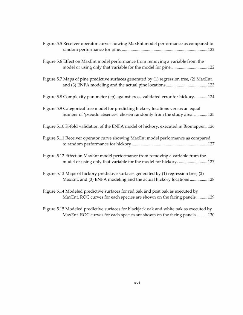
Figure 2.1 NMS ordination of pine plot communities. Community change through time is shown via vectors (a) that connect the same plot in 1977 and 2000.
Environmental variability is shown via the red overlay (b), indicating correlation of several environmental factors with axis 1 and sample year with axis 2. For simplicity, not all correlations are shown; see table 2.3(a) for all correlations of axes with other
measured factors.

37
Age class
pH
Axis 2
Axi
s 1
Hardwood Pine
Figure 2.2 NMS ordination of pine and hardwood plot communities using data
collected in 1977. Correlations of environmental variability is shown via the red overlays. For simplicity, not all correlations are shown; see table 2.3(b) for all
correlations of axes with other measured factors.

38
Axis 1
Axi
s 2
Year
pHCa Mg
Axis 1
Axi
s 2
Figure 2.3 NMS ordination of pine (black & light, open triangles) and hardwood (green & light, closed circles) plot communities. Light grey indicates resample plot position (2000). Community change through time is shown via vectors (a) that connect the same plot in 1977 and 2000. Environmental variability is shown via the red overlay (b), indicating correlation of several environmental factors with axis 1 and sample year with axis 2. For simplicity, not all correlations are shown; see table 2.3(c) for all correlations of axes with other measured factors.
Plots
Pine ∆ 1977 ∆ 2000
Hardwoood ● 1977 ○ 2000
2 2
1

39
Chapter 3: Presettlement vegetation of the North
Carolina Piedmont I

40
Introduction
When John Lawson, the English explorer, described the Piedmont of North
Carolina in the winter of 1701, he called it, “the Flower of Carolina”. From his journal,
we are able to glimpse a picture of the vegetation of presettlement North Carolina, from
“lofty Oaks” to “a prodigious overgrown Pine-Tree” (Lawson 1986). Some 30 years later,
while fixing the dividing line between North Carolina and Virginia, William Byrd and
Edward Ruffin would describe the vegetation as: “being clothed with large trees, of
poplar, hickory and oak” (Byrd and Ruffin 1841). It would be almost two centuries
before a more systematic survey was done of the trees of the North Carolina Piedmont
and great changes would have occurred on the landscape in the intervening time
(Pinchot and Ashe 1897). Ecologists of this century have also tried to imagine what the
forest community of presettlement vegetation looked like; in order to do so they used
remnant patches of forest – islands of unfarmed land in a landscape that had been
forever changed by European agriculture (Oosting 1942).
Characterizing the presettlement landscape
The use of witness trees to reconstruct presettlement forests is now a well
established field in ecology (Wang 2005). In areas surveyed after the U.S. general land
office (GLO) was established (1812), the process of mapping and analyzing pre-
settlement trees is relatively straightforward. It has been generally more difficult,

41
however, to reconstruct presettlement forests from areas of the country surveyed prior
to the GLO (i.e., most of the eastern U.S.).These colonial era surveys, or metes-and-
bounds surveys, were carried out differently from the more methodical GLO surveys.
When compared to studies done on more methodically surveyed areas,
published studies done using metes and bounds data are rare. For this reason, though
much more is known about presettlement forests of the Midwest and West, relatively
less is known about colonial forests from documentary sources. The exception to this is
some areas of the Northeast where township surveys have been used to reconstruct
presettlement forests (e.g., Cogbill et al. 2002). In the southeastern U.S., presettlement
records have been used to reconstruct forests in West Virginia (Abrams and McCay
1996), Pennsylvania (Whitney 1990, Abrams and Ruffner 1995, Black and Abrams 2001a,
b, Whitney and DeCant 2003, Black et al. 2006), southern Georgia (Cowell 1995, 1998),
and Alabama (Black et al. 2002, Foster et al. 2004). A map showing locations of witness
tree studies in the Southeast is shown in Figure 3.1. A notable gap in presettlement
survey studies is a large area between Georgia in the south and Pennsylvania in the
north (though some smaller scale, as yet unpublished, studies have examined few select
records in North Carolina; i.e., Frost 2000, Langley 2000). The mid-Atlantic region has
been particularly difficult to study via this technique because of the lack of organized
presettlement records.

42
The reconstruction of presettlement forests of the Carolina Piedmont via
standard pollen analyses is complicated by the lack of natural lakes in this region
(though see Russell 1993). Because of the lack of either pollen data or systematic
documentary evidence, ecologists have traditionally relied on extant stands to
approximate presettlement vegetation in this area. For example, Oosting (1942) wrote:
“when occasional hardwood stands are found which include trees 200-300 years of age
and show little evidence of recent disturbance, they must be accepted as samples of the
extensive hardwood forests which preceded the white man”. Oosting set the tone for
generations of ecologist who followed, who have generally assumed that oak and
hickory dominated forests are remnant of the original Piedmont forest and that pine
dominated forests are a result of well documented successional processes (Oosting 1942,
Bormann 1953, Peet and Christensen 1980b, Christensen and Peet 1981, Christensen and
Peet 1984).
Species-site relationships
Besides helping to understand compositional differences between presettlement
and current forests, presettlement records can help us understand species site
relationships before European land use. Species-site relationships can be altered by past
land use (Foster 1992, Motzkin et al. 1996, Motzkin et al. 1999, Foster et al. 2003).
Understanding species-site relationships is thus a first step in understanding the
controls on vegetation and how they may have changed since the beginning of

43
European land use. Presettlement records, by providing a snapshot of forests in time,
can also help suggest likely disturbance regimes patterning those forests (Cowell 1995).
Additionally, because they can be used to describe a large area, presettlement records
can provide an indication of different disturbance regimes across different sections of a
landscape, capturing, in effect, landscape heterogeneity (Wang 2005).
Characterizing small scale soil variation
Patterns of soil variation help control patterns of vegetation and these
relationships have been extensively studied both globally (Waide et al. 1999) and
regionally (Billings 1938, Oosting 1942, Peet and Christensen 1980a, Christensen and
Peet 1981, Palmer 1990). Soil site relationships have also been investigated for
presettlement vegetation; almost always this has involved using characteristics derived
from large scale soil and/or geologic base layers (e.g., texture, parent material, etc., Black
and Abrams 2001a). I use large scale soil maps (1:250,000; STATSGO) and similar scale
maps of underlying geology to define the physiographic provinces located on the study
site.
Large scale maps of soil properties are useful for looking at large scale patterns
of soil variation, but the within unit soil variation can be large, especially in areas
dissected by streams (Juracek and Wolock 2002). For mapping and analyses of stand
level (or in this case, tree level) data, 1:250,000 soil maps (STATSGO coverage) do not
resolve detail in a fine enough way to examine site-species relationships (Lathrop et al.

44
1995). Issues of scale have led to a recent effort to better use spatially explicit soil data at
finer resolutions on issues ranging from mapping water movement through soil profiles
(Di Luzio et al. 2004) to predicting future forest growth (Swenson et al. 2005). Although
an ongoing effort to map the soils of the entire United States at the county level has led
to widely available soil data at the 1:12,000 scale, a host of logistic issues confront the
researcher attempting to use these data (SSURGO) across several counties. County
surveys cannot be compared to each other without substantial pre-processing to deal
with inconsistent naming and mapping. Once these logistical issues are dealt with, soil
attributes must be joined to soil series. I focus my effort on two soil properties: fertility
and moisture (described below: Methods: Soils).
Objectives
In this chapter, I use a newly available dataset (Dobbs 2006) to explore
presettlement forests on the North Carolina Piedmont. I investigate (1) differences in
tree composition across the study site, and (2) species-site relationships with measured
landscape and soil factors. I place these novel results in a regional context and discuss
the role of possible disturbance regimes.

45
Methods
Study Area
The bounds of the study site encompass an area of ~4560 km2 lying in the central
Piedmont in North Carolina. The study area lies almost completely in what are now
Chatham, Durham, Granville, Orange, Person and Wake counties, and what was in the
presettlement time period (i.e., ~1750) Bladen, Granville, Johnston, and Orange counties.
The study area includes three major physiographic regions: the Carolina slate belt, the
Triassic basin, and the Raleigh belt (Figure 3.2). The slate belt bedrock consists mainly of
fine grained felsic metamorphic rocks (i.e., bedded argillites, felsic and mafic volcanics,
and schists). Carolina slate predominates, with thin but frequent basalt intrusions
(Daniels et al. 1999). Most soils in this province have deep silt loam surfaces. The Triassic
basin bedrock is composed mainly of shales, sandstones, and siltstones. Soils are mostly
heavily weathered Alfisols and Ultisols with high clay content in the subsoil. The
Raleigh belt, adjacent to the coastal plain to the east, lies atop bedrock that is primarily
acidic igneous such as, granite, granite gneiss, mica gneiss and mica schist (Calvert et al.
1980, O'Brien and Buol 1984, Daniels et al. 1999) Topography over the entire study site is
gently rolling with wide stream valleys intersecting higher ridges. Stream valleys in the
Triassic tend to be widest due to the more easily eroded nature of the bedrock and the
more gentle topography. The elevation across the study site differs somewhat; the

46
Triassic basin has the lowest mean elevation while the slate belt has the highest mean
elevation.
Prior to European arrival, the North Carolina Piedmont had been the home of
several Native American tribes. It is thought that populations during the 1600s were
near 20,000 in the region (Wood 1989). The region was largely depopulated of Native
Americans by the close of the 17th century due to smallpox and migrations (Ward and
Davis 1999). Though Europeans had explored the Piedmont earlier, European settlement
of the region began in earnest during the 1740’s and accelerated in the following decades
so that by 1770, European population in the area was approximately 40,000 (Wood 1989).
Though some property was already claimed by 1750, the studied record dates (1747-
1763) are coincident with the beginning of rapid European settlement of the Piedmont.
History & witness tree mapping
Presettlement trees were mapped using a reconstructed map of colonial era
surveys (Dobbs 2006). Originally, properties were surveyed by official surveyors at the
behest of a settler who was usually already living on the land. The claims process was
convoluted (and not totally germane) so I gloss over it here and provide only a
description of the important product: the survey document. The survey contained
written information about the size and the location of the property and a map of the
property showing important landscape features. The written text often described the
adjacent property owners as well. Spatial information in the written text most often
47
included rivers and streams, but could also include trails, topographic features, or
towns. Property corners were marked via some landscape feature, most frequently trees
but not uncommonly a post or a stream. The common names of these trees were
recorded in the survey. These survey plats, as well as associated documents such as
deeds, entries, and warrants were filed with the local land granting office (Mitchell
1993). The surviving documents for the study area were collected, transcribed, and
organized into a comprehensive and tailor made relational database (Dobbs 2006). From
the survey documents, GIS polygons were generated and then spatially mapped by
Dobbs (2006). The corners of these GIS polygons were converted to points, and each
point labeled with the tree name from the associated survey.
Landscape metrics
A suite of landscape metrics was calculated. In order to develop a metric of
landscape wetness, I calculated topographic relative moisture index (TRMI) modified
from Parker (1982). This index uses relative slope position, aspect, slope and curvature
to model water retention on the landscape. All metrics were calculated from a 30m
USGS digital elevation model (DEM) that was reprojected to WGS 1984 UTM Zone 17N.
The current landscape, however, is different in some important ways from the
presettlement one (e.g., lakes have been created by damming). In order to reconstruct
elevation as it might have been ca. 1750, I obtained bathymetry data for Jordan Lake
from the Army Corps of Engineers. This data layer was rasterized, reprojected,

48
converted to meters and then subtracted from the USGS DEM. All calculations were
done in ArcGIS 9.1 (ESRI, Redlands, CA, 2006). The relative slope position layer was
smoothed via the neighborhood statistics focal tool with a 3 x 3 cell neighborhood. In
addition, because TRMI was originally developed for areas with higher relief than the
North Carolina Piedmont, in the final calculation of TRMI, curvature values were not
used. Besides TMRI, I also calculated a measure that incorporates only wetness
measures, relative moisture index (RMI, Moore et al. 1993). This measure combines
water accumulation from upslope and the rate at which it drains. Both TRMI and RMI
gave similar pictures of wetness scores for the area; correlation between both rasters was
high.
Soil map
I obtained county-level soil data (SSURGO) for Alamance, Chatham, Durham,
Franklin, Granville, Johnston, Orange, Person and Wake counties from publicly
available data sources maintained by the USDA (http://soildatamart.nrcs.usda.gov/) in
all cases except Alamance, Durham, and Person counties. For these three counties,
tabular data were obtained from the USDA but the digitized maps were obtained from
the UNC GIS collection (Henley 2007). In order to use SSURGO data across counties, the
mapping unit ID (MUID) must be changed to the official series name (counties do not
use standardized MUIDs). After doing this, I merged all counties into one shape file
using ArcGIS 9.1 (ESRI, Redlands, CA, 2006) and reprojected to UTM. I exported the

49
data table of this layer file to R 2.4 (CRAN, 2006) and obtained the unique occurrences of
soil series for all nine counties (n=177).
In order to score soils for fertility, I created an ordinal variable (classes 1-4, Table
3.1) based on clay activity as measured by cation exchange capactity (CEC). In the
southeastern Piedmont, some soil series are practically devoid of exchangeable cations,
making these soils extremely nutrient poor environments for both natural vegetation
and agriculture. These soils, consisting of kaolinitic clays with kandic horizons, mark the
low end of activity for this ordinal variable (i.e., “subactivite”, class 1). At the highest
end of activity are soil series that contain high proportions of smectic clays and thus
have high CEC values (i.e., “active”, class 4). For soils in class 3 (“semiactive”) and 4,
clay activity was recorded from “activity” as reported by the Official Soil Series
Descriptions (OSD, NCRS 2007). “Activity” is defined by the OSD as ranges of CEC
(Table 3.1). The OSD does not list “activity” for kaolinitic soils, nor does it separate soils
with kandic horizons. In order to assign series with no “activity” rating (as reported by
the OSD), I used soil taxonomy to determine the presence of kandic horizons and the
reported mineralogy from the OSD to ascertain the presence of kaolinitic clays. Soils
with kandic horizons were scored as class 1 and those with predominantly kaolinitic
clays but without kandic horizons were scored as class 2 (“low activity”).
Soil moisture is frequently the result of a number of interrelated factors including
landscape position and soil texture (Brubaker et al. 1993, Brubaker et al. 1994). For this

50
study, I use an integrated proxy measure of soil moisture meaningful for plant
physiology: the average upper bound of saturated soil (i.e., free water) for a given soil
series as reported in the OSD (NCRS 2007). In this case, the variable reported by the OSD
is continuous, and no attempt was made to classify this variable.
Analyses
Species accumulation curves were constructed for each physiographic province.
In order to construct these curves, a given number of stems were sampled from all
possible stems and species richness was recorded. Sampling at each of nine values of
stems (i.e., 50, 100, 200, 300, 400, 500, 750, 1000, and 1250) was done 500 times to create
confidence intervals at each value. Not all provinces could be sampled at each number
of stems due to varying number of stems found in each physiographic province. In order
to compare species accumulation curves, a linear model was fit to the log means of each
sampling value for each province. Models were compared at a 95% confidence level.
To investigate species-site relationships, I used one of two techniques, depending
on whether the variable of interest was continuous or categorical. Species with more
than at least 5 records in any province were examined for association with landscape
factors (i.e., elevation, relative slope position, TRMI, RMI, aspect) and soil factors (i.e.,
clay activity, soil moisture). For continuous variables, the difference between the mean
value of a species in a given factor and province and the province mean for that factor
was calculated. This difference was then compared to 1000 randomized differences

51
calculated by selecting an equal number of trees at random from the given province and
calculating the difference between the new sampled mean and the province mean. The
proportion of times the actual difference exceeded the sample difference was used as the
p value for the randomized one-tailed t test (Manly 1997). For categorical variables, a
presence-absence contingency table was created. Independence of species distribution
with respect to categorical variable was tested via the G2 statistic (Sokal and Rohlf 1995).
Because a G2 score cannot be calculated for a value of 0, for any species where the value
of an observed box was 0, the value was changed to 0.001. Species that did not show
significant association with any categories were removed from further analysis. For
species that did show a significant association with factors, the corrected standard
residual (CSR) of the contingency table was taken (Strahler 1978) for further analysis.
Positive CSR scores indicate positive association with the variable in question and can be
compared across species.
Results
Tree composition
Surveyors identified a total of 2708 trees in 26 taxa, as well as 85 records of a
‘post’ or a ‘stake’. Surveyors did not record the name of 126 trees; these records were
considered ‘unspecified’. A total of 2582 trees were recorded with an associated taxon.
Numbers of trees in each physiographic province were 1417 in the Slate belt, 466 in the

52
Triassic basin and 784 in the Raleigh belt. Species richness in each province also differed:
25 taxa were recorded in the Slate belt, 18 in the Triassic basin and 14 in the Raleigh belt.
The species accumulation curve for each physiographic province is shown in Figure 3.3.
The curves for the Slate belt and for the Triassic basin are indistinguishable, whereas the
curve for the Raleigh belt is significantly different from the other two (p<0.001).
Species dominance varied by physiographic province (Table 3.2), though white
oak1 was abundant (~25% of the observed stems) in each of the three provinces. In the
Slate belt, white oak was the most common taxon; the next most common taxa were red
oak and hickory, each making up approximately 20% of the observed stems. In the
Triassic basin and the Raleigh belt, however, the most common taxon was pine, making
up close to a third of observed stems in both provinces. In contrast, pine made up less
than 5% of the stems in the Slate belt. Red oak and hickory were also common in the
Triassic basin and the Raleigh belt, but differed in their importance. In the Raleigh belt,
red oak comprised approximately 20% of stems, similar to the Slate belt. Hickory
comprised less than 10% of the stems in the Raleigh belt, much fewer than the
percentage found in the Slate belt. In the Triassic basin, red oak and hickory each
comprised approximately 10% of stems. No other taxon comprised more than 4% of the
stems in either the Triassic basin or the Raleigh belt. In the Slate belt, three more taxa did
comprise at least 4% of the stems: black oak (9%), blackjack oak and post oak (5% each;
1 Common names used in text, see Table 3.3 for scientific names

53
similar to the composition of pine stems). These trends were further examined by
examining the corrected standard residuals of species that showed a significant response
to ‘province’ (Figure 3.4). Clearly, many of the oak species are strongly associated with
the Slate belt, whereas pine is strongly negatively associated with the Slate belt and
positively associated with both the Triassic basin and (even more strongly) to the
Raleigh belt.
Trees of various sizes were recorded. Besides trees such as dogwood (six
recorded) and sourwood (one), which never reach the full canopy height, 182 trees were
identified by surveyors as ‘sapling’, ‘grub’, or ‘bush’. Each of the three physiographic
provinces had records of this type, but in differing percentages. Both the Slate belt and
the Triassic basin had approximately 8% of stems marked this way (113 and 37 stems,
respectively). In contrast, the Raleigh belt had far fewer stems marked this way (32
stems; 3.7%). In all of the tree records, one tree was recorded as ‘dead’. Several species
that are common in present-day forests occurred in surprisingly small numbers in the
historical data; among these taxa are maple (9 records, 0.3% total) and poplar (29
records, 1% of the total).
Species-site relationships
Many tree species showed significant interactions with landscape factors. Within
the Slate belt, hickory showed a significant difference from the sampled stems with
respect to TRMI (one tailed randomized t-test, p<0.05), RMI (p=0.01), and relative slope

54
position (p<0.01). The taxon mean for all three factors was smaller than the sampled
province mean, indicating that hickory associated with dryer than average sites with a
higher landscape position (i.e., associated with dryer hilltops). Similarly, pine was
associated with higher landscape position than average sampled stems in the Triassic
basin (relative slope position, p<0.05), though not in either of the other two
physiographic provinces. Black oak showed no significant differences from the
landscape in the Slate belt where it was common but did show significant association
with dryer sites (TRMI, p<0.05) in both the Triassic basin and the Raleigh belt. In the
Slate belt, the only province in which it occurs enough to test, beech associates
significantly with wetter than average (TRMI, p<0.01; RMI, p<0.01), and low landscape
position sites (relative slope position, p<0.01). Sweetgum also associates with wetter,
lower sites than average in the Triassic basin (RMI and relative slope position, p<0.05)
and is associated with significantly lower elevation sites in all three physiographic
provinces.
Across the entire study area, four taxa (white oak, water oak, pine and poplar)
showed significant associations with aspect class (Figure 3.5). All four showed negative
association with north aspect areas. White oak and pine, showed the strongest negative
associations to north aspect, and did not show particularly strong associations to the
other three aspect classes. Water oak showed strong association with south aspect areas.
Poplar showed strong negative association with south aspect areas and was also

55
significantly associated with low landscape position sites in both the Slate belt and
Raleigh belt (though, inconsistently, was associated with higher landscape position sites
in the Triassic basin) as well as with wetter sites in the Raleigh belt (TRMI, p<0.01).
Species-soil relationships
When compared among the surveyed locations, few tree species differed
significantly from the set of surveyed tree locations with respect to soil fertility
(measured via the ordinal variable clay activity) or moisture (measured as depth to
saturated soil). Two taxa, hickory and black oak, were associated with dryer sites (i.e.,
depth to saturated soil significantly greater than average of surveyed sites, p<0.05,
randomized t-test). Conversely, four species generally associated with alluvial soils were
found to be associated with wet sites (i.e., depth to saturated soil significantly less than
average of surveyed sites). These four species were beech and sweetgum (p<0.01), and
ash and water oak (p<0.05). Of special interest, pine was significantly associated (p<0.01)
with fertile soils in the Slate belt where it was not common. For illustrative purposes, a
representative map of slate belt pine locations is given in Figure 3.7. Pine locations in the
Slate belt are clearly clustered in alluvial areas with high fertility.

56
Discussion
Regional comparisons
The composition of the presettlement North Carolina Piedmont forests share
characteristics from previously reported presettlement forests of the eastern United
States. Large compositional differences between physiographic provinces has been
noted in forests of the Pennsylvania Piedmont and the Georgia Piedmont (Cowell 1995,
Black and Abrams 2001b, a). As would be expected, many species found in the North
Carolina Piedmont are also found in studies of presettlement vegetation in neighboring
regions.
The forests studied on the Pennsylvania Piedmont (Black and Abrams 2001b, a)
showed very similar percentages of white oak, which was also common across all
provinces in that study area. Their study site differed, however, in its almost complete
lack of red oak and pine taxa. Although the current distribution of red oak is throughout
the eastern U.S., it is possible that red oak was replaced by another species further north,
perhaps by black oak which was very common in that study. The lack of pine in that
area indicates a substantially different suite of early successional species present in the
presettlement community in that study area and perhaps differing disturbance regimes.
With studied forests located on the Georgia Piedmont (Cowell 1995), the North
Carolina Piedmont shares a similar percentage of all major taxa (pines, oaks, and
hickories) but a differing species mix. In the Georgia study, white oak is not nearly as

57
common (7.3% vs. 25%) and post oak is much more common (17.5% vs. 2.7%). The latter
difference may be explained in part by the greater percentage of drier sites examined in
that study, though post oak is not strongly associated with dryer sites in either study,
and may even have preference for wetter landscape areas. Additionally, the North
Carolina Piedmont is more similar to the reported presettlement composition of the
Georgia Piedmont than to the forest studied in Pennsylvania. This observation is borne
out by a Spearman rank correlation on the 10 most common species at each site: the
North Carolina and the Georgia sites are positively correlated (Spearman’s ρ=0.13),
whereas the North Carolina site is negatively correlated with the Pennsylvania site
(Spearman’s ρ= -0.84). Most species are present at all three sites, though there is some
obvious species turnover along the latitudinal gradient.
One notable difference between the three sites is the abundance of chestnut. In
the Pennsylvania site, this species makes up some 15% of the total stems surveyed,
although abundance ranges from a high of 17% in the ‘Piedmont uplands’ to a low of
0.5% in the ‘Piedmont lowlands’ (Black and Abrams 2001b). In the Georgia study,
Chestnut makes up a much smaller proportion of total trees, representing a significant if
minor species (~2% of the total stems sampled, Cowell 1995). In the present study, only
one tree was identified by surveyors as a chestnut (i.e., <0.1%). Chestnut has not been
assumed to have made up a major part of the North Carolina Piedmont presettlement
landscape and these results confirm that presumption.

58
Cross-physiographic province comparisons
The stark differences in species accumulation curves point to clear differences
among the three physiographic provinces. Previous work has posited that lower
diversity areas in the North Carolina Piedmont were a result of acidic igneous parent
material (Peet and Christensen 1988). The finding of significantly lower species richness
in the Raleigh belt compared with the other physiographic provinces supports that
contention.
The composition of the Carolina Slate belt was very similar to the presettlement
composition that Oosting (1942) described by relying on extant hardwood stands. The
other two provinces, however, differed substantially from this classic view – in large
part due to the high percentage of pines in both provinces. Because pines are indicative
of medium to large scale disturbance (Oosting 1942, Keever 1950, Bormann 1953), the
presence of high numbers of pine in these two regions points to different disturbance
regimes operating in the Triassic basin and the Raleigh belt as compared to the slate belt.
Understanding these differences are dealt with explicitly below (see subsection:
Disturbance).
Species-Site relationships
Many species showed consistent and expected relationships with measured
landscape factors. Species that preferred dryer, upland and higher elevation sites
included: black oak, blackjack oak, hickory, and (in the Triassic basin) pine. Species that

59
preferred wetter, lower elevation sites included water oak, willow oak and sweetgum.
Many trees such as red oak and post oak could not be associated with specific landscape
positions. These species may be near the optima of their geographic range and thus be
able to compete in a suite of environmental conditions within the North Carolina
Piedmont region.
Anomalously, pine was associated with dryer sites than random in the Triassic
basin but not significantly associated with any landscape factor in either of the other two
provinces. The explanation for this may lie in the fact that pine, rather than a species, is a
generic designation that likely includes more than one species. Modern as well as
historical studies have indicated that loblolly and shortleaf were predominant pine
species in the Piedmont range. The pine in the Triassic basin, associated with more
upland sites, was likely predominantly shortleaf. Older pines (>100 yrs old) found in this
area are predominantly shortleaf, providing further evidence for this assertion
(Christensen 1989). In the Raleigh belt, pine was not significantly different from random
sampling in terms of land form or wetness. However, the Raleigh belt was significantly
over sampled in wet, low landscape areas (more so than any of the three provinces). This
indicates that the predominant species of pine in the Raleigh belt may have been
Loblolly. Interestingly, when the association between pine and aspect was examined by
province, only the Triassic basin pines were significantly associated with East and West
aspect classes and negatively associated with the North aspect class, lending further

60
support to the possibility that the pines of the Triassic basin and the Raleigh belt were
not the same species. An early description of North Carolina’s timber reports similarly
about the different pine species in the ‘eastern granite areas’ and the ‘Jura triassic red
sandstone’ describing more shortleaf in the Triassic and more loblolly in the Raleigh belt
(Pinchot and Ashe 1897, 188)
Soil map and species-soil relationships
The nine-county soil map (Figure 3.6) represents a large extent, small scale
mapping of SSURGO data. Though efforts similar to this have been attempted, I know of
no similar project that has attempted to map soil series derived attributes over such a
large area of the North Carolina Piedmont. The map clearly reveals spatial patterns that
have been generally accepted (e.g., unfertile interfluves with high fertility fluvial zones
in the Raleigh belt) but also points at less generally appreciated soil fertility patterns
(e.g., high soil activity in the Triassic, Helms 2000).
Given that trees were almost certainly responding to soil characteristics, the lack
of significance in species – soil relationships for many species is puzzling. Several factors
may account for this including errors in tree positions, errors in mapping units,
mismatches in the scale of data, multi-species taxa, and the small number of soil
variables examined. Tree mapping errors are discussed in the previous chapter, and I
leave that discussion aside here and take up the others. First, soil series are inherently
variable and mapping them into homogeneous polygons is fraught with potential for

61
error and misclassification (Mueller et al. 2001). The scale of soil variation on the North
Carolina Piedmont is small (with significant differences occurring at the 1-100m2 scale,
Palmer 1990) whereas soil series are mapped without this granularity (100-1000m2 scale,
NCRS 2007). This scale mismatch compounds the potential for error when using these
soil data (Lin et al. 2005). It has been suggested that soil sampling and kriging, used in
combination with existing soil maps (Liu et al. 2006), could remedy some of these scale
related issues when trying to go from SSURGO scale soil data to the tree scale. Remote
sensing has also been used to map finer scale soil variations (Sullivan et al. 2005), and
this technique holds promise for improving efforts to map soil variation. It might also be
possible to field sample a select group of survey points, though this would then be
difficult to extrapolate to the whole landscape. It is unlikely that current fine scale soil
properties could be extrapolated backward in time to the presettlement era, given the
rate at which soil properties change and considering the intervening two plus centuries
of human land use, disturbance, and soil erosion, (Trimble 1974, Motzkin et al. 1996,
Richter and Markewitz 2001). This distance in time may also be responsible for the lack
of significant relationships found between species and soils. Although I selected
characteristics of soil that are likely quite persistent (Table 3.4, Richter in press), the
intervening two centuries and large scale erosion (Trimble 1974) may mean that it is
impossible to accurately portray small scale soil variation from ca. 1750.

62
The various species of pine and hickory were likely distributed along a soil
fertility gradient, but our ability to detect those relationships in these survey data is
hampered by the lack of species level identification. Shortleaf pine was likely most
abundant on dryer, less fertile upland sites (Pinchot and Ashe 1897, Billings 1938,
Bormann 1953) whereas loblolly was more commonly found mesic, fertile landscape
positions (Oosting 1942, Christensen 1989). In the Slate belt, the pines are located in
moist, low areas and almost certainly would have been loblolly (with perhaps some
individuals being Virginia pine, see Figure 3.7). These sites would have been good
agricultural areas, and are close to one of the best known archaeological sites in the
region2. Thus, Native American agriculture may well have played a role in the
distribution of Slate Belt pines. The overwhelming abundance of loblolly relative to
shortleaf on the current Piedmont landscape may be due in part to these initial
agricultural patterns, combined with 19th and early 20th century land use. European
settlers likely farmed the mesic, fertile and low areas first, and may also have abandoned
them first as agricultural production dropped there (Trimble 1974, Frankel 1984). These
disturbed, low areas would have created a landscape favorable to the spread of loblolly
throughout the North Carolina Piedmont. This changed landscape matrix, in turn,
2 The ‘Wall site’, located at a pronounced bend of the Eno River near the current town of Hillsborough, NC, is considered to be ‘Achonechy town’ visited by John Lawson on his explorations of North Carolina. The site was probably continuously inhabited by Siouan peoples from the 16th century to soon after Lawson’s visit in the first years of the 18th century (Ward and Davis 1999).

63
increased the seed rain from loblolly so that it overwhelmed shortleaf seed supply as
upper landscape areas were abandoned later on (but see also Christensen 1989).
Within the hickory taxon, Carya alba (L) (mockernut hickory, also C. tomentosa)
and C. glabra (pignut hickory) would have been the most common species, likely present
on a broad range of sites encompassing both dryer upland sites and moister
bottomlands. Other hickories would have included C. cordiformis (bitternut hickory)
which would have been most common in alluvial sites (Pinchot and Ashe 1897, Weakley
2006).
A broad range of site requirements also characterizes several of the oaks in the
North Carolina Piedmont region, especially Quercus alba, white oak, though it is
generally associated with slightly moister landscape positions. The requirements of post
oak are also quite broad, and though it is generally referred to as preferring dry upland
conditions (Pinchot and Ashe 1897, Oosting 1942, Weakley 2006). Oosting (1942)
reported finding it even in the most mesic remnant forest he surveyed and Coker (1945)
refers to it as a tree with a broad range of site tolerance.
Differing disturbance regimes across physiographic provinces
The obvious and significant differences in pine abundance across physiographic
regions are a clear indication of differing disturbance regimes. In the Piedmont region,
pine success has been linked to large scale disturbance events; they are excluded by
hardwoods in the case of small scale canopy disturbances (Billings 1938, Bormann 1953,

64
Peet and Christensen 1987). Other studies of presettlement vegetation have attributed
the presence of pines on the landscape to large scale fire, either human or natural caused
(Cowell 1995, Foster et al. 2004). The differences found in this study, given that they are
so clearly associated with physiographic section, point to some kind of soil mediated
process. This association with soil, in turn, implicates differing human land use, in
particular agriculture, as the likely cause of the differing disturbance regimes.
The native inhabitants of the North Carolina Piedmont grew corn, beans, and
gourds and practiced a form of swidden (slash and burn) agriculture through the area
(Ward and Davis 1999). Witness trees recorded in the 1750s would likely have started
growing some 50-200 years before, potentially toward the end of the 17th century. The
years of 1675 - 1700 was a time of large scale land abandonment as populations of
Native Americans living in the North Carolina Piedmont succumbed to epidemics
(Ward and Davis 1999, Davis 2002). The archeological evidence, however, does not
support large scale land abandonment simply because not enough settlements have
been found that would indicate populations large enough to have cleared substantial
portions of the Triassic basin and Raleigh belt (Davis 2002). Clearly, though, slash and
burn agriculture played some role creating a mosaic of open areas (Hammett 1992) that
might have been then been colonized by pine at the end of the 17th century. Another
possibility explaining the differing disturbance regimes is a vastly higher number of
hunting fires set by Native Americans at the beginning of the 18th century. Because of

65
political and economic pressure from the British, southern Indians turned to hunting
deer in much higher numbers at that time (Hudson 1981). These questions deserve more
interdisciplinary effort to clarify what ecologists, historians, and archaeologists can add
to each others’ stories.
Limitations
This study provides a novel picture of presettlement forests in the North
Carolina Piedmont. It is important to explicitly consider the limitations of this study
(and studies which rely on witness tree data more generally). I have briefly discussed
the differences between metes and bounds and more methodical surveys done later by
the GLO. The density of trees is lower in this study than in other studies, particularly
when compared with methodical surveys. The question of how coarse a resolution can
give a clear picture of presettlement forest has been taken up explicitly by Wang and
Larsen (2006) who found that in the extreme, even very low density surveys can
accurately reconstruct presettlement forests. Another, still open, question is the bias of
the surveyors themselves; i.e., did they choose trees non-randomly. I turn to that
question, among others, in the next chapter.

66
Summary
• The current study adds to our knowledge of the presettlement vegetation of the
southeastern U.S. showing that the North Carolina Piedmont was similar and
different to studied sites in southern Pennsylvania and central Georgia.
• The composition of the presettlement forest was both similar and different to that
imagined by Oosting and described by early explorers (Byrd and Ruffin 1841,
Oosting 1942, Lawson 1986).
• In particular, much of the forest was composed of oak and hickory, but the
abundance and spatial patterning of pine is surprising.
• Given our understanding on the controls of pine in the North Carolina Piedmont
and the spatial patterning of the pines themselves, their presence and pattern
point to differing disturbance regimes on the different physiographic provinces
of the North Carolina Piedmont.

67
Table 3.1 Scoring framework of clay activity and landscape position for SSURGO soil map used in the study modified from USDA soil classification system (NCRS 1999)
Ordinal value
Activity Cation exchange capacity (CEC)
Typical clay composition
1 Subactive
<< 0.24 Kandic clays*
2 Low activity <0.24 Kaolinitic clays*
3 Semiactive 0.24-0.40* Smectic clays
4 Active 0.40-0.60* Mixed mineralogy
*Characteristic used to define ordinal variable value

68
Table 3.2 Species occurrence by number and percent in each physiographic
province and by total.
Species Physiographic province Percent composition
Slate belt
Triassic basin
Raleigh belt Total Slate
belt Triassic basin
Raleigh belt Total
Apple 1 0 0 1 0.10% 0.00% 0.00% 0.00%Ash 6 3 5 14 0.40% 0.60% 0.60% 0.50%Beech 5 3 0 8 0.30% 0.60% 0.00% 0.30%Birch 1 0 0 1 0.10% 0.00% 0.00% 0.00%Black oak 128 16 12 156 8.80% 3.40% 1.40% 5.60%Blackgum 4 0 2 6 0.30% 0.00% 0.20% 0.20%Blackjack 68 11 13 92 4.70% 2.30% 1.50% 3.30%Chestnut 0 1 0 1 0.00% 0.20% 0.00% 0.00%Dogwood 3 1 2 6 0.20% 0.20% 0.20% 0.20%Hickory 275 55 69 399 18.80% 11.70% 8.00% 14.30%Hornbeam 1 0 0 1 0.10% 0.00% 0.00% 0.00%Maple 4 1 4 9 0.30% 0.20% 0.50% 0.30%Persimmon 2 0 0 2 0.14% 0.00% 0.00% 0.07%Pine 67 148 277 492 4.60% 31.60% 32.10% 17.60%Poplar 11 5 13 29 0.80% 1.10% 1.50% 1.00%Post oak 66 4 6 76 4.50% 0.90% 0.70% 2.70%Red oak 267 65 165 497 18.30% 13.90% 19.10% 17.80%Sassafras 1 0 0 1 0.10% 0.00% 0.00% 0.00%Sourwood 1 0 0 1 0.10% 0.00% 0.00% 0.00%Spanish oak 21 3 4 28 1.40% 0.60% 0.50% 1.00%Stake/post 57 16 12 85 3.90% 3.40% 1.40% 3.00%Sweetgum 20 5 9 34 1.40% 1.10% 1.00% 1.20%Turkey oak 2 0 0 2 0.14% 0.00% 0.00% 0.07%Unspecified 43 3 80 126 2.90% 0.60% 9.30% 4.50%Walnut 4 2 0 6 0.30% 0.40% 0.00% 0.20%Water oak 1 7 0 8 0.10% 1.50% 0.00% 0.30%White oak 398 117 191 705 27.20% 24.90% 22.10% 25.20%Willow oak 3 3 0 6 0.20% 0.60% 0.00% 0.20%Total count 1460 469 864 2793

69
Table 3.3 Common and scientific names of the species discussed in the present study. After Cowell (1995), Black and Abrams (2001b, 2001a), Weakley (2006), and Kartesz (1999)
Common name Scientific name Apple Malus spp. Ash Fraxinus americana, F. pennsylvanica Beech Fagus grandifolia Birch Betula nigra Black oak Quercus velutina Blackgum Nyssa sylvatica, N. biflora Blackjack oak Quercus marilandica Cherry Prunus americana, P. serotina Chestnut Castanea dentata Chestnut oak Quercus michaxii Chinquapin Castanea pumila, C. Ashei Dogwood Cornus florida, C. alternifolia Elm Ulmus alata, U. americana, U. rubra Hickory Carya cordiformis, C. glabra, C. ovalis, C. tomentosa Maple Acer saccharum, A. rubrum, A. saccharinum Persimmon Diospyros viginiana Pine Pinus echinata, P. taeda, P. virginiana Poplar Liriodendron tulipifera Post oak Quercus stellata Red oak Quercus rubra, Q. coccinea Sassafras Sassafras albidum Sourwood Oxydendrum arboreum Southern red (Spanish) oak Quercus falcata Sugar Celtis spp. Sweetgum (Gum) Liquidambar styraciflua Walnut Juglans nigra Water oak Quercus nigra White oak Quercus alba Willow oak Quercus phellos

70
Table 3.4 Soil properties generally grouped according to relative rate of change. After Richter (in press).
Readily altered 10 y
Relatively persistent 102 y
Persistent >103 y
Organic matter Texture Texture Acidity & salinity Illuvial clay Illuvial clay Exchangeable cations Mineral buffering Mineral buffering Redoximorphic features Redoximorphic features Rock content Bioavailable fractions of nutrients & contaminants
Duripans Plinthite
Duripans Plinthite
Surface charge Aggregation Rooting depth
Surface charge Aggregation Rooting depth
Surface charge

71
Whitney 1990
Black et al. 2002, Foster et al. 2004
Whitney and DeCant 2003
Abrams and McCay 1996
Schwartz 2007
Black et al. 2006
Cowell 1995, 1998
Black and Abrams 2001b, a
Abrams and Ruffner 1995
Abrams and Ruffner 1995
LegendNumber of witness tree records
235 - 2000
2001 - 20000
20001 - 50000
Figure 3.1 Regional map of witness tree studies done in the southeastern United States.
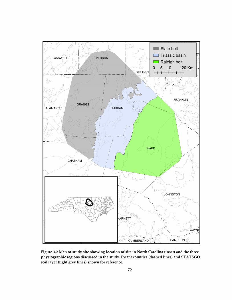
72
WAKE
LEE
HARNETT
CHATHAM
JOHNSTON
ORANGE
GRANVILLE
DURHAM
PERSON
FRANKLIN
VANCE
MOORE
ALAMANCE
CASWELL
SAMPSONCUMBERLAND
WARREN
WAYNE
Slate beltTriassic basinRaleigh belt
0 10 205 Km
Figure 3.2 Map of study site showing location of site in North Carolina (inset) and the three physiographic regions discussed in the study. Extant counties (dashed lines) and STATSGO soil layer (light grey lines) shown for reference.

73
Figure 3.3 Species accumulation curves for each physiographic province

74
Figure 3.4 Corrected standard residuals for several species significantly associated
with province

75
Figure 3.5 Corrected standard residuals for several species significantly
associated with aspect class
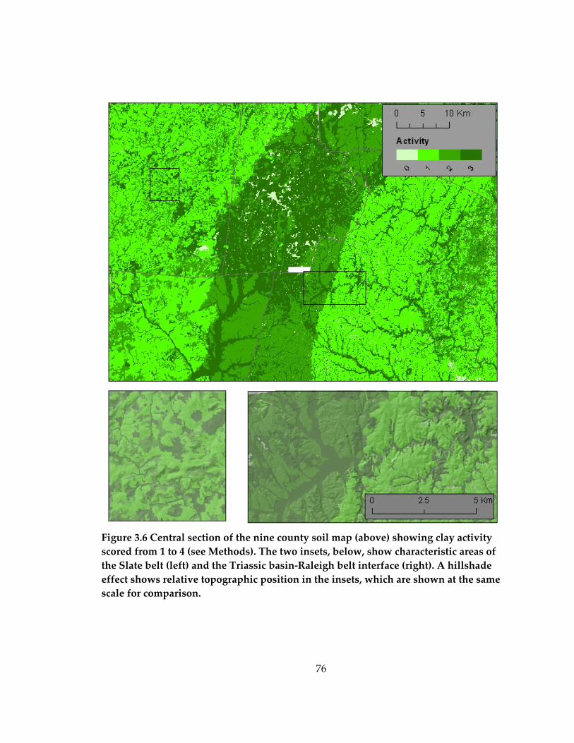
76
Figure 3.6 Central section of the nine county soil map (above) showing clay activity scored from 1 to 4 (see Methods). The two insets, below, show characteristic areas of the Slate belt (left) and the Triassic basin-Raleigh belt interface (right). A hillshade effect shows relative topographic position in the insets, which are shown at the same scale for comparison.

77
Figure 3.7 Locations of pines (▲) and other trees (●) for a portion of the study site (in the slate belt; see inset). Topography is indicated by hill shading, streams are shown by blue lines (—) and greenness increases with clay activity.

78
Chapter 4: Presettlement vegetation of the North
Carolina Piedmont II

79
Introduction
In this chapter I discuss the analyses of biases in dealing with metes-and-bounds
records for witness trees. The main types of bias treated are: the non random sampling
of the landscape by the colonial surveyors and the potential of those surveyors to be
biased in choosing or identifying trees.
Non random sampling of the landscape by surveyors
During European settlement of the North Carolina Piedmont, land was divided
somewhat haphazardly, as settlers claimed property wherever it suited them. Though
property boundaries are typically straight lines, many property edges follow river
courses and though properties were mostly contiguous this was not necessarily the case.
These differences from more methodical surveying methods (e.g., GLO surveys) make
interpreting data from such surveys more difficult. Witness tree density is a good
example of why it is more difficult to use metes and bounds surveys to study
presettlement vegetation. In GLO surveys, the density of witness trees is invariant across
geographic areas. In contrast, Black and Abrams (2001b) found that densities of witness
trees in a metes and bounds survey in Pennsylvania varied among physiographic
province. Moreover, GLO surveys sample the landscape pseudo-randomly whereas
metes and bounds surveys can over sample certain landforms if land was settled
preferentially with regard to landscape factors (Black and Abrams 2001b).

80
Surveyor bias in choosing trees
The topic of surveyor bias in choosing witness trees has rightly received at least
passing attention from nearly every study using this type of historical data. In the last
chapter I examined the non random placement of witness trees as compared to several
landscape metrics. In this chapter, I extend that analysis to non random placement with
respect to soil properties. I also deal with the more complex issue of surveyor bias in
choosing and identifying particular witness trees.
Surveyors may have preferentially chosen trees based on any number of factors,
including familiarity, size, ease of inscription, or economic value (Grimm 1984, Schulte
and Mladenoff 2001) and tests have been developed to assess for surveyor bias in
choosing corner trees (Bourdo 1956, Siccama 1971, Delcourt and Delcourt 1974). These
tests, however, are only applicable to GLO surveys that were collected using a more
standardized method of corner marking that included marking several trees at each
corner and recording the distance of each tree to the corner. GLO records generally have
the added advantage that they include ‘line descriptions’ that can be independently
compared to the composition of corner trees (Lorimer 1977, Whitney 1986). Because
metes and bounds records cannot be tested using these methods, researchers using
metes and bounds records have relied on the fact that surveyors recorded many
different tree species as evidence for the surveyors’ lack of bias.

81
Although this observation provides some evidence for lack of bias in choosing
trees, I propose a more quantitative test of surveyor bias in metes and bounds records
where the identity of the surveyor can be obtained. The identity of the surveyor is
generally available on the survey deed itself, and thus should not require much extra
effort in the way of data collection when working with records of this type. Two main
questions present themselves when trying to identify surveyor bias: (1) are surveyors
choosing species that are easily marked or in some way represent a circumscribed
sample of the total species of trees on the landscape, and (2) are surveyors consistent in
their identification (among surveyors and across time). To answer the first question, I
compare the number of species a given surveyor reports with the predicted number of
species he should have reported using the species accumulation curves generated in the
previous chapter. In order to answer the question about consistency, I take two
approaches. First, I compare the species found by surveyors to each other, working
under the assumption that significant inter surveyor differences may indicate bias (e.g.,
mistaken identification). Second, in cases with sufficient sample size, I compare the
species a surveyor marked in the winter with those marked by the same surveyor in the
summer. My assumption is that significant differences may be a reflection of a
surveyor’s tree identification skills. These tests for bias significantly add to the
usefulness of metes-and-bounds data by providing a stronger assessment of surveyors’
ability to accurately describe presettlement vegetation composition.

82
Methods
Analyses
Witness tree density was examined for variations by physiographic province. In
order to determine the ‘expected’ number of witness trees on each province, the
proportion of province area to total study area was multiplied by the total number of
witness trees. A χ2 statistic was calculated for each physiographic province to determine
the significance of differences between observed and expected number of trees. In order
to determine if property size explained witness tree density, acres of property was
regressed on density of witness trees in a given province.
To determine whether sampling across the landscape was biased with respect to
the overall study site, the sampled tree points were compared with an equal number of
randomly generated points drawn from a possible 20,000 points. Random points were
generated using Hawth's Analysis Tools for ArcGIS ver. 3.26 (Beyer 2006). After
generation, these points were then sub-sampled to get 100 random subsets of points. For
continuous variables, the difference between means of these distributions and the true
province mean were compared to the difference between the mean of the surveyor
sampled points and the true province mean (randomized t test, Manly 1997). For
categorical variables, all 20,000 random sample points were used to get expected values
and a χ2 statistic was calculated to determine the significance of differences between
observed and expected makeup of tree position.

83
Surveyor bias
Surveyors were analyzed separately by province. Species accumulation curves
were generated as described in Chapter 3, and 95% confidence intervals calculated. For
each surveyor who surveyed more than 30 trees in a given province, I calculated the
expected number of species that should have been reported, along with the upper and
lower bounds for the expectation. This expectation was then compared to the actual
number of species found by that surveyor. Data were plotted and compared graphically.
To assess for consistency of species identification among surveyors, I compared
the species composition reported by surveyors who surveyed more than 30 trees in a
province to each other, by individual province. To assess for internal surveyor
consistency, I compared the species reported by surveyors who had surveyed at least 30
trees in both the summer and the winter. Summer (leaf on) was defined as April to
October, and winter (leafless) as November to March.
Results
Surveyed witness tree variations
Density of witness trees varied by landscape province. The Slate belt was
surveyed most intensively of the three provinces with a density of 0.77 trees/km2,
significantly more than the expected sampling intensity (Table 4.1). By contrast, the
Triassic basin was sampled significantly less than expected, with only 0.40 trees/km2.

84
The Raleigh belt was sampled at a density of 0.57 trees/km2, similar to the average
density over the whole study area of 0.60 trees/km2. Average property size explains little
of this variation in density (R2=0.03, p<.001).
Surveyed locations were found to be non random with respect to the landscape
for some measured factors, though for the most part, differences were small. In all three
provinces, valley bottoms and alluvial areas were over sampled and ridge positions
were under sampled relative to the landscape overall. Mid slope positions were slightly
under sampled (Table 4.2). These differences were most pronounced in the Raleigh belt.
Over sampling of the low landscape position sites shifted mean TRMI and RMI values of
sampled sites upward (i.e., wetter sites were preferentially sampled) relative to the mean
TRMI and RMI values for the entire province significantly (though for RMI in the Slate
belt, the difference was non-significant). For wetness value, these differences were
relatively minor (e.g., ~5% differences in means for TRMI, 20% differences in means for
RMI). Mean elevation of surveyed points was significantly less than that found via
random sampling in the Triassic basin and the Raleigh belt (one tailed randomized t-
test, p<0.01). In the Raleigh belt, this likely has to do with the aforementioned over
sampling in valley bottoms. In the Triassic basin, however, this may have to do with the
fact that most of the surveyed points are located in the southern half of the province
where elevation is lower. In terms of aspect, surveyed locations were indistinguishable
from random sampling.

85
Using data from the soil map (Figure 3.6) I compared the properties of the overall
landscape with the surveyed points with respect to soil properties. When compared to
the random sample of points, tree locations were biased with respect to clay activity and
soil moisture factors; compared to the landscape average, trees were surveyed in areas
with higher than average clay activity and moisture. This difference was strongest in the
Raleigh belt. This result reinforces the findings above that indicate that trees in the
Raleigh belt were found in and near the alluvial, high fertility locations more frequently
than would be expected at random.
Surveyor bias
No significant differences were found between the expected number of species a
surveyor reported based on the number of trees he surveyed and the number of species
he actually reported (Figure 4.1). The most prolific surveyor, William Churton, observed
more species than would be expected in each province, though in no case was the
difference significant. Only two other surveyors, Wade and Caswell surveyed more than
20 trees in more than one province. Neither of them showed consistent behavior by
either over reporting or under reporting species relative to the expected.
When compared to each other, surveyors reported similar tree compositions in
each province (Table 4.3). In particular, I looked at differences in percentages between
oaks, given that these species can be difficult to identify in the field. Although in the
Slate belt Caswell reports a higher percentage of red oak than either of the other two

86
surveyors, the percentages that he reports for other species (including black oak) are in
line with the other surveyors. In the Raleigh belt, where there are more surveyors to
compare, there are somewhat large differences (~10%) between surveyors’ reporting
percentage. In no instance was one surveyor’s reported species composition markedly
different from the others. Differences between the surveyors’ reported species
composition are likely due to natural heterogeneity in the vegetation communities in the
Raleigh belt itself and the particular locations that each surveyor worked in.
Only four surveyors surveyed enough trees in any province to compare
percentages of trees marked in the summer against those marked in the winter. When
compared to themselves at different parts of the year, marked tree percentages changed
very little (Table 4.4). Churton, with the largest ‘sample size’, has almost identical
percentages in the summer and the winter indicating that surveyors were likely
consistently identifying trees without the use of leaf features.
Discussion
Biased sampling of the landscape
The settlement processes of the colonial Piedmont were non-random; people
made decisions on where to locate property based on a suite of factors that took into
account, among others, people, transportation, and the quality of the land. This process
is reflected in the biased nature of the witness tree sample when compared to the total

87
landscape. In particular, the surveyed trees were significantly more likely to be
associated with low landscape position, wet sites (whether measured via TRMI or soil
moisture). These sites are also associated with highest clay activity in each province and
thus, arguably, with higher overall soil fertility. These patterns are likely a result of
preferential settlement patterns by the first European settlers of the North Carolina
Piedmont. The settlers would have quickly identified high fertility areas, and these
would have been the sites of the first properties. These sites were likely the same ones
that had been farmed by the Native Americans, and this preferential pattern of
settlement has been described from patterns of soil erosion (Trimble 1974) and current
vegetation (Taverna et al. 2005b). It is important to note, however, that this story is
complicated by the correlated nature of soil and landscape factors in the North Carolina
Piedmont. Low landscape positions tend to be more protected, have higher soil fertility,
and have soil with free water near the surface, making assigning one cause for
settlement patterns difficult.
The decreased fertility of the Raleigh belt relative to the other provinces may also
serve to explain the relatively higher oversampling of the bottomlands in that province,
that is, with significantly lower fertility in upper landscape positions, settlers might have
preferentially chosen properties around streams and low landscape positions. Though
this pattern is most strongly recorded in the Raleigh belt, in general Piedmont soils have

88
higher native fertilities in bottomland slope positions and this is reflected in the
oversampling of the bottomlands in all provinces.
Surveyor bias
I found little evidence for surveyor bias in the study area and surveyors
accurately portrayed the composition of the forests they surveyed. This is good news for
ecologists working with colonial era documents trying to reconstruct forest patterns.
This does not mean that all metes and bounds surveys should be accepted before similar
testing, and I propose that the tests presented here should become standard where
possible for testing metes and bounds records. Since carrying out these tests requires
only a minimal extra effort in terms of data collection, the benefits of carrying out these
tests far outweigh the benefits. These tests do not eliminate the possibility of all biases.
In particular, if all surveyors shared similar biases in choosing trees, these tests would
not detect them. The number of surveyors who surveyed sufficient numbers of trees to
compare against each other was limited, this limitation also prevented more robust
comparisons of surveyors.
A picture of the colonial surveyor as a semi-expert plant biologist emerges from
these data and available historical documents. For most surveyors, little historical
material is available, but I was able to find material pertaining to William Churton. He is
described by contemporaries as “excessively scrupulous” and “certainly a reasonable
man” (Engstrom 1979). After his career as a surveyor, he was involved in politics in his

89
home in Hillsborough, where the main street is now named after him. It is likely that
surveyors were quite accurate in their descriptions, in Ohio researchers were able to
verify the identification of GLO surveyors with extant trees (Whitney 1994).

90
Table 4.1 Differing witness tree density by landscape province
# of witness trees Physiographic province
Total area (km2) Expected Observed
χ 2 test statistic
P value
Slate belt 1896.7 1157 1460 35.2 <.0001 Triassic basin 1172.1 715 469 51.4 <.0001 Raleigh belt 1510.7 921 864 1.8 0.1750

91
Table 4.2 Non random sampling of the landscape by colonial surveyors
Landscape position Province
High Mid Low χ2 test statistic P value
Observed 754 408 298 8.4 <0.05 Slate belt Expected 824 387 247 Observed 225 121 123 7.1 <0.05 Triassic basin Expected 260 116 92 Observed 432 229 203 13.4 <0.01 Raleigh belt Expected 495 221 147

92
Table 4.3 Witness tree species percentages by surveyor and physiographic province
Slate belt Triassic basin Raleigh belt Surveyor Churton Lewis Caswell Churton Caswell Caswell Churton Young Haywood Hunter
Ash 0.3% 0.0% 2.4% 0.8% 0.0% 0.0% 0.0% 0.6% 0.6% 0.0% Beech 0.4% 0.0% 0.0% 0.8% 0.0% 0.0% 0.0% 0.0% 0.0% 0.0%
Black oak 8.7% 11.1% 9.8% 4.0% 0.0% 0.0% 7.6% 0.6% 0.6% 2.1% Blackgum 0.2% 0.0% 2.4% 0.0% 0.0% 0.0% 1.3% 0.3% 0.0% 0.0% Blackjack 4.8% 13.9% 0.0% 2.7% 2.4% 0.0% 3.8% 1.9% 1.8% 0.0% Dogwood 0.2% 0.0% 0.0% 0.3% 0.0% 0.0% 0.0% 0.3% 0.6% 0.0% Hickory 18.5% 19.4% 14.6% 10.7% 21.4% 5.1% 2.5% 9.9% 9.7% 7.1% Maple 0.2% 0.0% 0.0% 0.3% 0.0% 0.0% 0.0% 0.0% 0.0% 2.9% Pine 5.0% 0.0% 0.0% 31.5% 40.5% 40.5% 26.6% 23.1% 43.6% 40.7%
Poplar 0.8% 0.0% 0.0% 0.3% 0.0% 1.3% 5.1% 0.9% 1.8% 0.0% Post oak 4.6% 0.0% 2.4% 0.8% 0.0% 0.0% 0.0% 0.0% 0.0% 4.3% Red oak 17.9% 16.7% 29.3% 12.3% 19.0% 21.5% 22.8% 18.8% 12.7% 21.4%
Spanish oak 1.5% 2.8% 2.4% 0.5% 2.4% 0.0% 1.3% 0.6% 0.0% 0.7% Stake 4.1% 0.0% 2.4% 4.3% 0.0% 0.0% 2.5% 3.1% 0.0% 0.0%
Sweetgum 1.2% 0.0% 4.9% 1.3% 0.0% 3.8% 1.3% 0.0% 1.2% 1.4% Water oak 0.1% 0.0% 0.0% 1.9% 0.0% 0.0% 0.0% 0.0% 0.0% 0.0% White oak 27.4% 27.8% 26.8% 26.1% 11.9% 10.1% 22.8% 24.1% 24.2% 17.1%Willow oak 0.2% 0.0% 0.0% 0.8% 0.0% 0.0% 0.0% 0.0% 0.0% 0.0% Unspecified 2.8% 8.3% 2.4% 0.3% 2.4% 17.7% 2.5% 15.7% 3.0% 2.1% Total stems 1287 36 41 375 42 79 79 324 165 140

93
Table 4.4 Witness tree species percentages by surveyor, physiographic province, and surveyed season, summer (April – October) and winter (November – March)
SurveyorSeason summer winter summer winter summer winter summer winter summer winter summer winterApple 0.0% 0.2% 0.0% 0.0% 0.0% 0.0% 0.0% 0.0% 0.0% 0.0% 0.0% 0.0%Ash 0.3% 0.3% 0.8% 0.7% 0.0% 0.0% 0.0% 0.0% 0.8% 0.0% 0.0% 0.0%Beech 0.3% 0.5% 0.8% 0.7% 0.0% 0.0% 0.0% 0.0% 0.0% 0.0% 0.0% 0.0%Birch 0.0% 0.2% 0.0% 0.0% 0.0% 0.0% 0.0% 0.0% 0.0% 0.0% 0.0% 0.0%Black oak 8.6% 8.8% 3.8% 4.4% 5.5% 12.5% 0.0% 0.0% 0.4% 1.6% 2.7% 1.9%Blackgum 0.3% 0.0% 0.0% 0.0% 1.8% 0.0% 0.0% 0.0% 0.4% 0.0% 0.0% 0.0%Blackjack 5.0% 4.6% 2.9% 2.2% 3.6% 4.2% 0.0% 0.0% 1.9% 1.6% 0.0% 0.0%Dogwood 0.3% 0.2% 0.4% 0.0% 0.0% 0.0% 0.0% 0.0% 0.4% 0.0% 0.0% 0.0%Hickory 18.1% 18.9% 11.3% 9.6% 3.6% 0.0% 5.4% 4.8% 11.2% 4.7% 0.0% 9.7%Maple 0.2% 0.3% 0.4% 0.0% 0.0% 0.0% 0.0% 0.0% 0.0% 0.0% 5.4% 1.9%Pine 5.4% 4.5% 32.9% 28.9% 30.9% 16.7% 27.0% 52.4% 21.2% 31.3% 48.6% 37.9%Poplar 1.1% 0.5% 0.0% 0.7% 7.3% 0.0% 2.7% 0.0% 1.2% 0.0% 0.0% 0.0%Post oak 4.7% 4.5% 1.3% 0.0% 0.0% 0.0% 0.0% 0.0% 0.0% 0.0% 0.0% 5.8%Red oak 17.1% 18.9% 12.1% 12.6% 20.0% 29.2% 18.9% 23.8% 20.0% 14.1% 21.6% 21.4%Sourwood 0.0% 0.2% 0.0% 0.0% 0.0% 0.0% 0.0% 0.0% 0.0% 0.0% 0.0% 0.0%Spanish oak 1.8% 1.1% 0.8% 0.0% 0.0% 4.2% 0.0% 0.0% 0.8% 0.0% 2.7% 0.0%Stake 5.9% 2.2% 2.5% 7.4% 1.8% 4.2% 0.0% 0.0% 3.8% 0.0% 0.0% 0.0%Sweetgum 1.8% 0.6% 1.3% 1.5% 1.8% 0.0% 5.4% 2.4% 0.0% 0.0% 0.0% 1.9%Unspecified 2.4% 3.2% 0.4% 0.0% 3.6% 0.0% 32.4% 4.8% 14.6% 20.3% 2.7% 1.9%Walnut 0.5% 0.2% 0.4% 0.0% 0.0% 0.0% 0.0% 0.0% 0.0% 0.0% 0.0% 0.0%Water oak 0.2% 0.0% 1.3% 3.0% 0.0% 0.0% 0.0% 0.0% 0.0% 0.0% 0.0% 0.0%White oak 25.1% 29.8% 25.8% 26.7% 20.0% 29.2% 8.1% 11.9% 23.5% 26.6% 16.2% 17.5%Willow oak 0.3% 0.2% 0.4% 1.5% 0.0% 0.0% 0.0% 0.0% 0.0% 0.0% 0.0% 0.0%Total stems 662 625 240 135 55 24 37 42 260 64 37 103
Slate Belt Triassic basin Raleigh beltChurton Caswell Young Hunter

94
Figure 4.1 Number of tree species reported by surveyor in each province plotted against log number of trees surveyed. Surveyors are indicated by red circles (○) identified by their last name. Each graph shows the predicted line and confidence intervals (dashed) based on randomized sampling of the data at several sampling levels (○).

95
Chapter 5: Reconstructing the historical landscape
using modeling methods

96
Introduction
Recent advances in modeling species distributions have shed light on where
species are found and the processes that pattern those distributions (Wiens and Graham
2005, Lutolf et al. 2006, Austin 2007). The insights gained from species models have been
applied to important questions in the fields of conservation, population viability
analysis, invasive species, and planning networks of protected areas (Elith et al. 2006).
Modeling presettlement vegetation
The spatially explicit type of data provided by witness tree records has been used
to model presettlement tree distribution (Fralish et al. 1991, Leahy and Pregitzer 2003,
Wang 2007). This has been done in part to turn somewhat sparse data (the points of the
witness tree locations themselves) into a better picture of how forest communities might
have looked in the presettlement time period. Three techniques have been primarily
implemented to model presettlement vegetation: (1) synthetic plots, (2) direct spatial
interpolation or (3) a combination of both (Cowell 1995, Black et al. 2002, Cogbill et al.
2002). Each of these approaches has significant weakness in both theory and practice,
although they have produced suitably interpretable results. The methodology of
creating synthetic plots consists of binning species into plots based on their occurrence
in similar environmental conditions. Little ecological theory supports this approach.
Results from this method are further suspect because the researcher must specify apriori

97
which factors will be important for species (i.e., how plots are synthesized) and must
also choose breaks to determine what will define a “plot”. This might be an issue, for
example, if different results are obtained depending on whether plots are split into four
or eight cardinal directions (i.e., N/W/E/S vs. N/NE/E/SE/S/SW/W/NW), but the choice of
where to split (often continuous) variables is many times dictated not by ecological
considerations but by the need to have a suitable sample size in each “plot” (Cowell
1995, Black and Abrams 2001a). Direct spatial interpolation makes fewer theoretical
leaps, but also has two main drawbacks. As an averaging technique, it must be used
over large areas; thus limiting its ability to discern meso-scale detail (i.e., <1 km2, Black et
al. 2002). Second, the technique inherently treats the absence of information as
information about absence, a critical error with data of this type. The final major
drawback with these techniques is the inability to easily validate results, making
understanding the errors associated with these models difficult if not impossible.
Putting habitat models in context
Data from presettlement witness trees is similar, conceptually, to data frequently
encountered in museum collections or herbaria (although the quality, in numbers of
records and accuracy of associated spatial location, is often much better for
presettlement witness tree records). A witness tree recorded at a given location indicates
the presence of that species at that location, but the absence of records does not imply
the absence of that species at a given location. Recent interest in making use of data

98
found in museums and herbaria for a variety of applications, as well as a broader
realization that ecological data in general often lack proof of species absence, has led to a
renewed focus on developing modeling techniques that can make use of presence only
data (Guisan and Thuiller 2005, Elith et al. 2006, Phillips et al. 2006).
The general aim of habitat models is to predict a range of ‘good habitat’ for a
target species using environmental (and sometimes community) correlates important for
that species. Conceptually, all habitat models rely on the concept of the realized niche
(Hutchinson 1957) and our presumed ability to classify the habitat preferences of a given
species and distinguish it from non-habitat. When absence data are available, modeling
approaches have attempted to distinguish good habitat (locations where the species is
known to occur) from bad habitat (locations where it is known to be absent). Some of the
new methods for working with presence-only data are reapplications of models which
have been extensively applied to model habitat using presence-absence data (e.g.,
generalized linear models, GLMs). For these models to work with presence only data,
“pseudo absences” (randomly sampled locations from the landscape) are generated and
used in the place of known, field sampled, absences. Other techniques, in particular,
maximum entropy (Phillips et al. 2006) and Ecological-Niche Factor Analysis (ENFA,
Hirzel et al. 2002a) were specifically designed to deal with presence only data. Two
recent reviews of presence only modeling techniques list over a dozen different models
useful for modeling presence only data which have been developed in the last decade

99
alone (Guisan and Thuiller 2005, Elith et al. 2006). The interpretation of presence only
models differs from the general interpretation of presence-absence habitat models.
Whereas with presence-absence data the results of the model indicate ‘good habitat’ vs.
‘bad habitat’, in presence only modeling the results of the model indicate better habitat
relative to the general study area. This makes habitat models using presence data
sensitive to the extent of the study (Hirzel et al. 2002a) and generally better able to
predict species with more specialized habitat requirements (Elith et al. 2006).
All habitat models work under the questionable assumption that a species’
realized niche is approximately equal to its fundamental niche (Hutchinson 1957, Guisan
and Zimmermann 2000, Wiens and Graham 2005, Araujo and Guisan 2006). Although
this is likely the case some of the time, the discrepancies between the realized niche and
the fundamental niche can be significant. Species may not be distributed in all suitable
locations for many reasons, including dispersal limitations, competition, or disturbance
(Pulliam 2000, Svenning and Skov 2005). These factors make the realized niche look
smaller than the fundamental niche, but the scale of the difference cannot be determined
using modeling techniques (Ibáñez et al. 2006). The reverse problem, where the realized
niche could appear bigger than the fundamental niche, can also occur; this would be the
case where a species is present in a given habitat but is unable to reproduce there (i.e.,
sink habitats, Pulliam 1988). Both of these issues are problems for all habitat models, but
may be exacerbated in presence only models (Hirzel et al. 2002a). Despite these

100
theoretical shortcomings, these models provide an important way to look at
presettlement data and are supported by both statistical theory and empirical testing
(Zaniewski et al. 2002, Robertson and Barker 2006, Pearson et al. 2007). Finally, model
misspecifications, when they can be discovered, are themselves important clues.
Patterns of misspecifications can be helpful in elucidating what information might be
missing from a model that may have helped to better predict species occurrence
locations. This information, in turn, can often give clues to important processes that
pattern species distribution in the real world (Pearce and Ferrier 2000).
Presence based modeling techniques
Classification trees
Like GLMs, classification trees have a long history in ecology for predicting
habitat using presence-absence data (Breiman et al. 1984, Urban 2002). They have been
used especially when species responses may be non-linear and in particular spatially
differentiated (Taverna et al. 2005b, Olivier and Wotherspoon 2006). This application has
been especially useful to predict binary responses (e.g., habitat/non-habitat) but can be
easily coerced to provide misclassification rates at each leaf node (Moore et al. 1991,
Urban et al. 2002). Another benefit of tree based models is that they can be reprojected
into geographical space through the use of simple conditional statements generated
from the trees.

101
Model implementation is executed through a one-step forward search algorithm
that looks at all possible splits of the data along all input factors (Urban 2002). The
model splits the data to minimize variance in the daughter branches. Since the process of
splitting itself can go on in until all nodes are split, models are generally overfit and
need to be pruned. Tree pruning is done via comparison with cross validated data that
assigns a cost to each split. Though the exact size of the final tree is somewhat subjective,
trees are usually pruned to minimize size while maintaining maximum cross validated
information.
Ecological-Niche Factor Analysis
Ecological-Niche Factor Analysis (ENFA), as implemented in Biomapper v3.1
(Hirzel et al. 2002a, Hirzel et al. 2002b) is specifically designed for presence only data
and for the analysis of ecological data. Because of this, it is the model most clearly
related to ecological theory, specifically based on the multi-dimensional niche concept
proposed by Hutchinson (1957). ENFA works similarly to principal components analysis
(PCA, Pearson 1901, Hotelling 1933), extracting from the environmental variables
orthogonal “marginality” and “specialization” factors. Marginality is defined as the
difference between the mean of a given species and the mean of the landscape on a
given environmental factor. Specialization is defined as the ratio of the standard
deviation of a landscape factor over the entire study area to the standard deviation of
the species in that same factor (Hirzel et al. 2002a, see Figure 5.1). By calculating

102
marginality and specialization in multi-dimensional space, the ENFA technique
approximates the Hutchinsonian niche (Hirzel et al. 2002a). Factor analysis is used to
remove colinearity in the environmental variables and to find values for marginality and
specialization. In contrast to PCA, where axes are chosen to maximize the variance
explained on each axis, factor analysis is used in ENFA to separate marginality (first
axis) and specialization (succeeding axes) in order to make interpretation of axes
ecologically relevant (Hirzel et al. 2002a). The calculated niche space is then reprojected
into geographic space using environmental data from the study area.
Maximum entropy
Maximum entropy techniques are based on the information principle, first stated
by Jaynes (1957), that the approximation of an unknown distribution should be
constrained only by known constraints but that, where constraints are unknown, the
distribution should tend toward entropy. Simply stated, we must not make unfounded
assumptions about a given distribution. The maximum entropy approach has been used
in numerous fields and is the subject of active research for applications to machine
learning (Phillips et al. 2006); its application to modeling species distributions is quite
recent (Elith et al. 2006). In the case of modeling a species, the distribution we are
modeling is the location, in environmental factor space, of the species of interest
(Phillips et al. 2006). Modeling the distribution takes a uniform probability of occurrence
and subjecting it to constraints based on information derived from the relation between

103
known locations of species presence and the environmental variables of interest. MaxEnt
calculates a probability distribution for every grid cell across the entire study site and
operates in a generative way (adding conditions to the entropy distribution) in an
iterative fashion (Phillips et al. 2006). MaxEnt models tend to overfit data, and so cross
validation of the data (where part of the data is used to model habitat and the remaining
data is used to validate the model) is integrated into the MaxEnt software (Phillips et al.
2006).
Modeling presettlement vegetation as presence data
In this chapter I use the presettlement witness tree data and compare three
techniques of presence-only modeling using two taxa, hickory and pine in order to both
(1) determine the usefulness of presence only modeling techniques for witness tree data
and (2) shed light on the likely patterns of pine and hickory distribution across the study
area. I use these two taxa to compare across modeling treatments because both provide
about equal numbers of records, but differ markedly in their fidelity to landscape sites.
In chapter 3 and 4, I showed that hickory was present over the entire study area in
approximately similar proportions across all three physiographic provinces and with no
clear patterns relating to wetness. Pines, however, were primarily found in wetter and
lower areas (particularly in the Raleigh belt), and were restricted almost completely
from the Slate belt. Comparing these two species across models allowed comparing
species that were found to behave quite differently.

104
Methods
Data processing
Most data processing was done in ArcGIS 9.1 (ESRI, Redlands, CA, 2006) using
other software obtained for specific tasks in the data processing workflow. The
BIOMAPPER software (Hirzel et al. 2002b) requires rasters in IDRISI (Clark Labs,
Worcester MA) format and the translation of the ESRI grid format to IDRISI format was
done using Grid2Idrisi 1.0 (Marinoni and Schäuble 2005). Data layers that were used are
as described in previous chapters, except for two changes. First, in order to smooth data
layers, I increased the grid cell size of the digital elevation model (DEM) from ~30 x 30m
to ~90 x 90m. This made models run more smoothly and had the added benefit of
preventing small errors in tree positions from unduly influencing the model (Brotons et
al. 2004, Engler et al. 2004). Other landscape factors were calculated from this new DEM
as before. Second, in order to use it as a continuous factor, I transformed aspect using
the following formula after Beers et al. (1966):
T.Aspect = - (cos (45-aspect))
where aspect is in degrees.
Categorical tree model
Regression trees were modeled in R v2.3 (CRAN) using the external library rpart.
Data consisted of species records (NPINE = 499, NHICKORY = 392), an equal number of

105
‘absences’ drawn from 20,000 random points and the associated environmental scores
for each location. First, a tree was created with no penalty for overfitting (i.e., complexity
parameter, cp=0) and the cross validated standard errors were examined. Trees were
pruned at the point where the relative error as a function of tree size reached a plateau.
The pruned tree was used to develop a set of predictive rules which were then mapped
onto geographic space using ArcGIS. Rather than map presence/absence, however, I
mapped percentage presence at each leaf of the tree, giving a smoother final map more
suitable for interpretation as a predictive surface. Two runs of the model were
performed, one using soil factors available for most of the modeling extent, another
without any soil factors. Environmental factors used by the model runs are given in
Table 5.1.
ENFA model
All ENFA (Hirzel et al. 2002a) models were performed in Biomapper v 3.2
(Hirzel et al. 2002b). Because I was unable to use categorical variables with the
Biomapper program, not all variables were used to model hickory and pine habitat
(Table 5.1). Hickory and pine locations were converted to raster cell formats to match the
necessary inputs for the Biomapper model. First, a covariance matrix was calculated.
Using species locations, factor analysis proceeds by partitioning marginality and
specialization. As in PCA, earlier axes explain more variance and it is usually
unnecessary to use all recovered factors to create the final habitat map. For each species I

106
used the number of factor axes that explained at least 80% of the factor variation. Habitat
suitability maps are calculated from the factor axes and species position location within
Biomapper and outputted as grids with values from 0 (poor predicted habitat) to 100
(best predicted habitat). Validation is executed through k fold validation (Boyce et al.
2002) which partitions the species points into k mutually exclusive sets. I used 10 as the
value of k. For each validation step, k, a habitat suitability model is computed (leaving
out the validation set) and this model is compared to the data that is left out. By
comparing the performance of these models, predictive power can be assessed.
Performance is gauged by binning the map into i classes and comparing the proportion
of validation points in each bin (Pi) to the proportion of the map area covered by that bin
(Ei), where i is equal to the bin number; I used i=4 (Hirzel et al. 2002b). A measure of
model goodness is obtained by dividing Pi by Ei (Boyce et al. 2002, Hirzel et al. 2006). If
the habitat map does no better than random, the variance of Pi/Ei is high and includes 1,
whereas if the model is good, low scores should have low Pi/Ei values and high habitat
scores should have high Pi/Ei scores.
MaxEnt model
MaxEnt models were performed using MaxEnt v 2.3 (Phillips et al. 2006). The
MaxEnt model begins by giving every raster cell in the study area an equal probability
of containing the species of interest. Through an iterative process the model fits
functions to each environmental layer to improve the fit of the predictive surface to the

107
known presence points. The possible shapes of the functions that are fit to the
environmental variables are extremely broad and are fit so that the summation of all
predictive surface grid cells must sum to the empirical mean of that layer. MaxEnt
model default values for convergence level (0.00001) and maximum iterations (500) were
used for model runs. Background data points were selected from 20,000 random points
and associated environmental data, but a maximum of 10,000 points were used by each
run. As with the categorical tree model, two runs were performed for each species
tested, one using soil factors available for most of the modeling extent, another without
any soil factors. Environmental factors used by the model runs are given in Table 5.1.
Validation is carried out by computing a modified receiver operator curve as described
in Phillips et al. (2006). The area under the curve (AUC) gives a metric of goodness of fit,
where a model that did no better than random has an AUC = 0.5 and a model that
perfectly predicts the data has an AUC = 1.
Results
Pine
Regression tree model
After visual inspection of complexity parameter (cp) against model size, a nine
leaf tree was chosen for pine (cp = 0.02, Figure 5.2). The resulting tree uses elevation and
RMI to make all splits in the tree (Figure 5.3). RMI is used at seven nodes, indicating a

108
potentially non-linear response to moisture in pine. A map produced from the
regression tree is given in Figure 5.7 (lower left).
ENFA model
Pine had a marginality score of 0.399 and a specialization score of 1.067
indicating that the ENFA model found some difference between the species and
background scores on transformed environmental variables. The specialization score
close to unity indicates that the range of the species compared to the background is very
similar (specialization is a ratio of standard deviations). Three factor axes were retained
from the ENFA analyses of pine. The first axis is chosen by factor analysis to explain all
marginality, so its value for how much of the marginality variance it explains will
always be 100%. The first axis also explains some of the specialization variance, and
together the three axes represent 84% of the specialization. Axes correlations with
environmental factors and the weights of each axis are shown in Table 5.2a. The ability
of the model to predict left out data in the k-fold validation step was high, with a plot of
Pi/Ei showing positive slope and low variance (Figure 5.4). A predictive surface map for
pine was generated and is shown in figure 5.7 (upper right).
MaxEnt model
The MaxEnt model for pine had a ROC that indicated it did a better job at
predicting the data than a random grab (Figure 5.5). The MaxEnt model produced a map
that accurately captured the higher abundance of that species in the Triassic basin and

109
the Raleigh belt (Figure 5.7, upper left). Areas with high predictive value were found
mostly in low, high wetness value areas, though in the Triassic basin the model found
high predictive surface values for more upland interfluves. The most important variable
used in modeling the pines, as evidenced by large differences in model performance
when using vs. not using this data (jackknife test, Figure 5.6) was RMI. The function that
the MaxEnt fit to RMI was highly nonlinear and indicated a complex response to
wetness values (data not shown).
Hickory
Regression tree model
After visual inspection of complexity parameter (cp) against model size, a 16 leaf
tree was chosen for hickory (cp = 0.013, Figure 5.8). The resulting tree uses province,
elevation, RMI and (at one node) TRMI to make all splits in the tree (Figure 5.9). As in
the regression tree for pine occurrences, RMI is used at many nodes, in this case 12.
Again, this indicates a potentially non-linear and quite complex response to moisture in
hickory. A map produced from the regression tree is given in Figure 5.13 (lower left).
ENFA model
Hickory had a marginality score of 0.186 and a specialization score of 1.01
indicating that the ENFA model found little difference between the species locations and
background scores on transformed environmental variables. The specialization score
close to unity indicates that the range of the species compared to the background is very

110
similar. As with pine, three factor axes were retained and represent 82% of the
specialization. Axes correlations with environmental factors and the weights of each axis
are shown in Table 5.2b. Prediction of the model was low, with a plot of Pi/Ei showing
no slope and high variance (Figure 5.10). A predictive surface map for hickory was
generated and is shown in Figure 5.13 (upper right)
MaxEnt model
For hickory, the MaxEnt model produced a map that accurately captured the
higher abundance of that species on the Slate belt but also showed it present in both of
the other provinces (Figure 5.13, upper left). The ROC curve for this model differs from
random (Figure 5.11) and the total area under the ROC curve (AUC) is similar to that
found for the pine model (AUCPINE = 0.93; AUCHICKORY = 0.92), indicating similar
predictive power. The most important variable used in modeling hickory, as with pine,
was RMI (jackknife test, Figure 5.12). The function that the MaxEnt fit to RMI was highly
nonlinear and indicated a complex response to wetness values (data not shown).
Other species
Maps made using the MaxEnt model for several other species of oak (red oak,
post oak, blackjack oak, and white oak) are shown in Figures 5.14 and 5.15 with their
associated ROC curves. All models had an AUC above 0.5; in general AUC was lower
for species with fewer observations.

111
Discussion
Modeling techniques
Several recent papers have attempted to compare presence only modeling
methods against each other (Zaniewski et al. 2002, Engler et al. 2004, Elith et al. 2006,
Phillips et al. 2006). All of them do so at much larger scales, and without discussing the
likely biological meanings of particular predictions, or what differences in modeling
approaches might illuminate in terms of understanding the drivers of species
occurrence. This study takes a much smaller scale approach, looking at only a few
species with a few methods. As such, this study serves less as a test of modeling
techniques than as an attempt to apply several promising methods to real data which is
both sparse and messy. It is thus fitting, since I am more concerned here about the likely
occurrence of presettlement species than about comparing modeling details, that I spend
most of the discussion making intra species comparisons rather than looking at models
across species.
Pine modeling
All three models of pine accurately captured the very different abundance of
pine in each physiographic province. Each model, however, did so differently. The
ENFA model was unable to use physiographic province/geology directly, but it is
evident from the high correlation of elevation to the primary axis of variation that the

112
ENFA model used this variable as a proxy for province. Because of this, the ENFA
model presents a picture of pine habitat closely linked to topographic variation.
Interestingly, the lowest areas on the landscape, both in the Triassic basin and the
Raleigh belt are marked unsuitable in the ENFA model. This is likely a model
misspecification, and probably results from using elevation as the primary predictor
variable. The other two models, the categorical tree and the maximum entropy model,
do a better job using biologically significant variables to generate predictive surfaces for
pine. It is significant that both of these models were able to fit different functions to
different geographic areas and that both did so. The maximum entropy model used
geology/province directly as a categorical factor, and the regression tree model used
elevation as a surrogate for this split, but both models fit different responses to
environmental factors depending on where on the landscape a prediction was for. The
output maps from both of these models were very similar and both used complex
functions to fit RMI as the main predictor variable. The complex and non-linear response
to relative moisture index may be an indication of the multi species taxon that ‘pine’
represents (i.e., Pinus taeda, P. echinata, P. virginiana, and likely small numbers of P.
palustris).
The major difference between the two predictive surface maps is that the
regression tree model places higher predictive values on the upland areas of the Triassic
basin, in line with the analyses done in Chapter 2 and with the hypothesis that shortleaf

113
was present in higher numbers in the Triassic basin. This is seen in the tree itself (Figure
5.3) as well, where after the first split, the higher part of the landscape (left branch of the
tree) branches with higher RMI values (wetter) generally have less pine. The differences
between the predictive surfaces generated with the maximum entropy and the
regression tree methods, however, are slight and may reflect particularities of each
method more than anything else.
Hickory modeling
In contrast to pine, hickory showed less difference between physiographic
provinces in the study area, consistent with the idea that hickory was found across the
study area in roughly similar proportions (although abundance was highest in the Slate
belt, something that the models picked up). The ENFA model found little specialization
in hickory against the background landscape; this undoubtedly influenced the low
predictive power of that model. The maximum entropy and regression tree techniques
produced similar predictive surface maps for hickory and, as for the pine maps, used
similar environmental variables. Both models used RMI as a key variable for mapping
hickory. The complex and non linear response of hickory to RMI may signal, as with
pine, the multi species nature of the hickory taxon. It may also signal the broad habitat
preferences of hickory, and its widespread presence in the study area (Pinchot and Ashe
1897, Coker 1945, Weakley 2006).

114
Model validation
There is not yet a consensus way to validate models made using presence only
data and each model uses a different validation method. It is plausible that all presence
only models could be compared with the model proposed by Phillips (2006) that uses
ROC curves with a modified definition of specificity. I have not undertaken that
analysis, however, and use the validation method used by the author of each technique.
It has also been suggested that comparing the minimum area needed by each model to
encompass all known occurrences of a given species might serve as a way to compare
presence only models (Zaniewski et al. 2002, Phillips et al. 2006). Ecologically, however,
there is little justification for this validation technique: a model that predicts all
occurrences with the least area may or may not be a better predictor of species habitat
than one that uses more area – this is more a test of a model’s expressiveness (sensu Elith
et al. 2006) than anything else; small predictive areas may mean that model are overfit to
the data.
Limitations
The proliferation of methods to model presence data should not shift attention
away from the weaknesses inherent in all implementations of niche based modeling.
Although niche based modeling is now widely used by both the scientific and policy
communities, the technique has major weaknesses, including the treatment of the
realized niche as the fundamental niche (Pacala and Hurtt 1992, Pearson and Dawson

115
2003). Like all modeling of this type, these techniques force researchers to make apriori
assumptions of what environmental variables are important to a given species. Results
can be influenced by what data are available, what data are used, and what scale is
chosen for analysis. Finally, all predictive modeling based on describing the relationship
of a species with environmental factors is unable to account for the effects of
disturbance. Unless researchers have a access to information about disturbance, it is
impossible to incorporate disturbance into these models.
Summary
• Presence only modeling techniques proved tractable and useful for examining
the patterns of presettlement trees in the North Carolina Piedmont
• Several techniques were able to accurately predict likely presettlement species
distributions, with the caveat that (with presence-absence models) it is difficult to
estimate how well they are performing.
• MaxEnt and regression tree models did better than the ENFA modeling
technique at capturing both geographically mediated processes and species that
were not ‘specialized’ as compared to the background landscape – both of these
techniques hold promise for further modeling of presettlement tree data

116
Table 5.1 Explanatory environmental layers used for each model run. Results are not given for all model runs.
Model Environmental factor Provincea Elevationc RMIc RSPc T.Aspectc Soil
activityo Distance to activec Upperc
ENFA x x x x
Regression tree 1 x x x x x x x x
Regression tree2 x x x x x
MaxEnt1 x x x x x x x x
MaxEnt2 x x x x x
Notes: a categorical, o ordinal, c continuous, 1 run with soil factors, 2 run without soil factors

117
1 2 3Elevation -0.975 -0.009 0.078RMI 0.125 -0.114 -0.508RSP 0.152 0.579 0.462TASP 0.047 -0.4 0.096TRMI 0.09 -0.701 0.716
Factor axis
1 2 3Elevation 0.957 -0.162 0.068RMI -0.172 -0.522 0.048RSP 0.119 -0.07 0.637TASP -0.059 0.603 -0.16TRMI 0.19 0.577 -0.75
Table 5.2 Correlation between first three factor axes and environmental factors from the Biomapper model using pine (a) and hickory (b)
(a)
(b)

118
Figure 5.1 Graphical simplification of ‘marginality’ and ‘specialization’ as defined implemented in the Biomapper model (Figure from Hirzel et al. 2002a).

119
Figure 5.2 Complexity parameter (cp) against cross validate error for pine. By convention, categorical trees are pruned when the value of cross validated error reaches a plateau

120
Figure 5.3 Categorical tree model for predicting pine locations versus an equal number of ‘pseudo absences’ chosen randomly from the study area. The tree is read from the top where each node represents a conditional statement and true responses to the conditional go left. Nodes are marked both by the binary ‘present’ or ‘absent’ and by the number of points described by that node with pines on the right side of the slash (/) and pseudo absences on the left.

121
Habitat suitability10095908580757065605550454035302520151050
Pred
icte
d/Ex
pect
ed ra
tio
2
1
Figure 5.4 K-fold validation of the ENFA model of pine as executed in Biomapper. The axes are described in the text (see Methods: Biomapper). Points indicate means and vertical lines are ±1 S.D. in four bins (0-25,25-50,50-75,75-100) of habitat suitability score

122
Figure 5.5 Receiver operator curve showing MaxEnt model performance (red line) as compared to random performance (blue line) for pine.
Figure 5.6 Effect on MaxEnt model performance from removing a variable (y axis) from the model (light blue bars) or using only that variable for the model (dark blue bars) for pine.
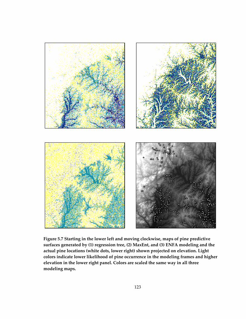
123
Figure 5.7 Starting in the lower left and moving clockwise, maps of pine predictive surfaces generated by (1) regression tree, (2) MaxEnt, and (3) ENFA modeling and the actual pine locations (white dots, lower right) shown projected on elevation. Light colors indicate lower likelihood of pine occurrence in the modeling frames and higher elevation in the lower right panel. Colors are scaled the same way in all three modeling maps.

124
Figure 5.8 Complexity parameter (cp) against cross validated error. By convention, categorical trees are pruned when the value of cross validated error reaches a plateau

125
Figure 5.9 Categorical tree model for predicting hickory locations versus an equal number of ‘pseudo absences’ chosen randomly from the study area. The tree is read from the top where each node represents a conditional statement and true responses to the conditional go left. Nodes are marked both by the binary ‘present’ or ‘absent’ and by the number of points described by that node with hickory on the right side of the slash (/) and pseudo absences on the left.

126
Habitat suitability10095908580757065605550454035302520151050
Pred
icte
d/Ex
pect
ed ra
tio2
1
Figure 5.10 K-fold validation of the ENFA model of hickory as executed in Biomapper. The axes are described in the text (see Methods: Biomapper). Points indicate means and vertical lines are ±1 S.D. in four bins (0-25, 25-50, 50-75, 75-100) of habitat suitability scores

127
Figure 5.11 Receiver operator curve showing MaxEnt model performance (red line) as compared to random performance (blue line) for hickory (Phillips et al. 2006).
Figure 5.12 Effect on MaxEnt model performance from removing a variable (y axis) from the model (light blue bars) or using only that variable for the model (dark blue bars) for hickory.

128
Figure 5.13 Starting in the lower left and moving clockwise, maps of hickory predictive surfaces generated by (1) regression tree, (2) MaxEnt, and (3) ENFA modeling and the actual hickory locations (white dots, lower right) shown projected on elevation. Light colors indicate lower likelihood of hickory occurrence in the modeling frames and higher elevation in the lower right panel. Colors are scaled the same way in all three modeling maps.

129
Figure 5.14 Modeled predictive surfaces for red oak (top) and post oak (bottom) as executed by MaxEnt. ROC curves for each species are shown on the facing panels.

130
Figure 5.15 Modeled predictive surfaces for blackjack oak (top) and white oak (bottom) as executed by MaxEnt. ROC curves for each species are shown on the facing panels.

131
Chapter 6: Conclusion

132
Conclusions
This dissertation provides new insights into the importance of history on the
ecology of the North Carolina Piedmont. In particular, I show that over both the decadal
and the century scale, the process of vegetation change is constant and strongly
influenced by human behavior. The forests of the North Carolina Piedmont are both
strikingly different and remarkably similar to how they were several hundred years ago.
At a smaller scale and rate of change, the same applies to the Duke Forest over the past
few decades. Studies like this one make clear the key role that humans will increasingly
have to play as landscapes become more fragmented and require more intensive human
management. Management decisions, both taken and ignored, will determine the state
of our forests in the coming decades and centuries. The processes of human population
growth in general and the even more rapid increase of North Carolina’s population are
unlikely to slow in the near future. These pressures, and the forest fragmentation
associated with them, are rapidly changing the matrix in which our forests operate, the
processes they are exposed to, and what they will like in the future. In a sense, studies
like this provide a long term perspective on subjects that are often examined at relatively
short time scales. I hope that readers of this dissertation, above all, will come away with
the understanding that we are also setting initial conditions today for a future that we
can only guess at. Our actions today in setting these conditions will likely have effects
that ripple outward for decades and centuries to come.

133
Summary
The goal of this dissertation was to increase understanding of vegetation and
community change in the North Carolina Piedmont. My main findings include the
following:
Chapter 2
• The understory communities of successional forest in the Duke Forest are
changing. Although total species richness stayed relatively constant through the
23-year step, herb richness declined with a concomitant increase in woody
richness.
• Plot composition change was remarkably consistent and this change was not
correlated with any measured stand or environmental factors.
• Community-level changes are consistent with previously reported changes in the
understories of mature, hardwood-dominated stands in the Duke Forest,
suggesting that landscape-scale drivers may be more important than within-
stand successional processes in determining change in herbaceous composition.
• Combined with growing evidence from other studies, our study indicates that
forests in the temperate region may be experiencing changes different from those
predicted by successional chronosequence studies.

134
Chapter 3
• The composition of the presettlement forest was both similar and different to that
imagined by Oosting and described by early explorers (Byrd and Ruffin 1841,
Oosting 1942, Lawson 1986).
• Much of the forest species was oak and hickory, but the abundance and spatial
patterning of pine is surprising.
• The spatial patterning of the pines is likely a result of differing disturbance
regimes on the different physiographic provinces of the North Carolina
Piedmont, and these differences may have been mediated by humans.
Chapter 4
• Fertile soil sites were preferentially surveyed, likely reflecting early settlement
patterns on the North Carolina Piedmont
• Methods for determining surveyor bias were developed and little to no evidence
for surveyor bias either in choosing species or identifying species was found.
Chapter 5
• Several techniques were able to accurately predict likely presettlement species
distributions, with the caveat that it is difficult to estimate how well they are
performing

135
• MaxEnt and regression tree models did better than the ENFA modeling
technique at capturing both geographically mediated processes and species that
were not ‘specialized’ as compared to the background landscape – both of these
techniques hold promise for further modeling of presettlement tree data

136
Literature Cited
Abrams, M. D. 2003. Where has all the white oak gone? Bioscience 53:927-939. Abrams, M. D., and D. M. McCay. 1996. Vegetation site relationships of witness trees
(1780-1856) in the presettlement forests of eastern West Virginia. Canadian Journal of Forest Research-Revue Canadienne De Recherche Forestiere 26:217-224.
Abrams, M. D., and C. M. Ruffner. 1995. Physiographic Analysis Of Witness-Tree
Distribution (1765-1798) And Present Forest Cover Through North Central Pennsylvania. Canadian Journal of Forest Research-Revue Canadienne De Recherche Forestiere 25:659-668.
Araujo, M. B., and A. Guisan. 2006. Five (or so) challenges for species distribution
modelling. Journal of Biogeography 33:1677-1688. Austin, M. 2007. Species distribution models and ecological theory: A critical assessment
and some possible new approaches. Ecological Modelling 200:1-19. Bakker, J. P., H. Olff, J. H. Willems, and M. Zobel. 1996. Why do we need permanent
plots in the study of long-term vegetation dynamics? Journal of Vegetation Science 7:147-155.
Bayliss-Smith, T., E. Hviding, and T. Whitmore. 2003. Rainforest composition and
histories of human disturbance in Solomon Islands. Ambio 32:346–352. Beers, T. W., P. E. Dress, and L. C. Wensel. 1966. Aspect transformation in site
productivity research. Journal Of Forestry 64:691-692. Bellemare, J., G. Motzkin, and D. R. Foster. 2002. Legacies of the agricultural past in the
forested present: an assessment of historical land-use effects on rich mesic forests. Journal of Biogeography 29:1401-1420.
Beyer, H. L. 2006. Hawth's Analysis Tools for ArcGIS. Bickel, K. A. 2001. Land use, disturbance, and the spread of non-native plant species in a
Piedmont forest ecosystem. Ms. Duke University.

137
Billings, W. D. 1938. The structure and development of old field shortleaf pine stands and certain associated physical properties of the soil. Ecological Monographs 8:436-499.
Black, B. A., and M. D. Abrams. 2001a. Analysis of temporal variation and species-site
relationships of witness tree data in southeastern Pennsylvania. Canadian Journal of Forest Research-Revue Canadienne De Recherche Forestiere 31:419-429.
Black, B. A., and M. D. Abrams. 2001b. Influences of native Americans and surveyor
biases on metes and bounds witness-tree distribution. Ecology 82:2574-2586. Black, B. A., H. T. Foster, and M. D. Abrams. 2002. Combining environmentally
dependent and independent analyses of witness tree data in east-central Alabama. Canadian Journal of Forest Research-Revue Canadienne De Recherche Forestiere 32:2060-2075.
Black, B. A., C. M. Ruffner, and M. D. Abrams. 2006. Native American influences on the
forest composition of the Allegheny Plateau, northwest Pennsylvania. Canadian Journal of Forest Research-Revue Canadienne De Recherche Forestiere 36:1266-1275.
Bormann, F. H. 1953. Factors determining the role of loblolly pine and sweet gum in
early old-field succession in the Piedmont of North Carolina. Ecological Monographs 23:339-358.
Bourdo, E. A., Jr. 1956. A Review of the General Land Office Survey and of Its Use in
Quantitative Studies of Former Forests. Ecology 37:754-768. Boyce, M. S., P. R. Vernier, S. E. Nielsen, and F. K. A. Schmiegelow. 2002. Evaluating
resource selection functions. Ecological Modelling 157:281-300. Breiman, L., J. H. Friedman, R. A. Olshen, and C. J. Stone. 1984. Classification and
Regression Trees. Wadsworth and Brooks/Cole, Monterey. Brotons, L., W. Thuiller, M. B. Araujo, and A. H. Hirzel. 2004. Presence-absence versus
presence-only modelling methods for predicting bird habitat suitability. Ecography 27:437-448.

138
Brubaker, S. C., A. J. Jones, K. Frank, and D. T. Lewis. 1994. Regression-Models for Estimating Soil Properties by Landscape Position. Soil Science Society of America Journal 58:1763-1767.
Brubaker, S. C., A. J. Jones, D. T. Lewis, and K. Frank. 1993. Soil Properties Associated
with Landscape Position. Soil Science Society of America Journal 57:235-239. Byrd, W., and E. Ruffin. 1841. The Westover Manuscripts: Containing the History of the
Dividing Line Betwixt Virginia and North Carolina; A Journey to the Land of Eden, A. D. 1733. Petersburg: Edmund & Julian C. Ruffin. Documenting the American South. 2001. University Library, The University of North Carolina at Chapel Hill. http://docsouth.unc.edu/nc/byrd/byrd.html.
Calvert, C. S., S. W. Buol, and S. B. Weed. 1980. Mineralogical characteristics and
transformations of a vertical rock-saprolite-soil sequence in the North Carolina piedmont: I. Profile morphology, chemical composition and mineralogy and II. Feldspar alteration products-their transformation through the profile. Soil Science Society of America Journal 44:1096-1112.
Christensen, N. L. 1989. Landscape history and ecological succession on the Piedmont of
North Carolina. Journal of Forest History 33:116-124. Christensen, N. L., and R. K. Peet. 1981. Secondary forest succession on the North
Carolian Piedmont. Pages 230-245 in D. West, H. Shugart, and D. Botkin, editors. Forest Succession: Concept and applications. Springer-Verlag, New York.
Christensen, N. L., and R. K. Peet. 1984. Convergence During Secondary Forest
Succession. Journal Of Ecology 72:25-36. Cogbill, C. V., J. Burk, and G. Motzkin. 2002. The forests of presettlement New England,
USA: spatial and compositional patterns based on town proprietor surveys. Journal of Biogeography 29:1279-1304.
Coker, W. C. 1945. Trees of the Southeastern states. University of North Carolina Press,
Chapel Hill. Cooper, S. R., S. K. McGlothlin, M. Madritch, and D. L. Jones. 2004. Paleoecological
evidence of human impacts on the Neuse and Pamlico Estuaries of North Carolina, USA. Estuaries 27:617-633.

139
Cote, S. D., T. P. Rooney, J. P. Tremblay, C. Dussault, and D. M. Waller. 2004. Ecological impacts of deer overabundance. Annual Review Of Ecology Evolution And Systematics 35:113-147.
Cowell, C. M. 1995. Presettlement Piedmont Forests - Patterns Of Composition And
Disturbance In Central Georgia. Annals Of The Association Of American Geographers 85:65-83.
Cowell, C. M. 1998. Historical change in vegetation and disturbance on the Georgia
piedmont. American Midland Naturalist 140:78-89. Daniels, R. B., S. W. Buol, H. J. Kleiss, and C. A. Ditzler. 1999. Soil systems in North
Carolina. North Carolina State University, Raleigh, NC. Davis, R. P. S., Jr. 2002. The cultural landscape of the North Carolina Piedmont at
contact. Pages 135-154 in R. Ethridge and C. Hudson, editors. The transformation of the Southeastern Indians 1540-1760. University Press of Mississippi, Jackson.
Davison, S. E., and R. T. T. Forman. 1982. Herb and shrub dynamics in a mature oak
forest - A 30-year study. Bulletin of the Torrey Botanical Club 109:64-73. Delcourt, H. R., and P. A. Delcourt. 1974. Primeval Magnolia-Holly-Beech Climax in
Louisiana. Ecology 55:638-644. Di Luzio, M., J. G. Arnold, and R. Srinivasan. 2004. Integration of SSURGO maps and
soil parameters within a geographic information system and nonpoint source pollution model system. Journal of Soil and Water Conservation 59:123-133.
Dobbs, G. R. 2006. The Indian Trading Path and colonial settlement development in the
North Carolina Piedmont. PhD. University of North Carolina, Chapel Hill. Drayton, B., and R. B. Primack. 1996. Plant species lost in an isolated conservation area
in Metropolitan Boston from 1894 to 1993. Conservation Biology 10:30-39. Druckenbrod, D. L., and H. H. Shugart. 2004. Forest history of James Madison's
Montpelier Plantation. Journal of the Torrey Botanical Society 131:204-219. Dupouey, J. L., E. Dambrine, J. D. Laffite, and C. Moares. 2002. Irreversible impact of
past land use on forest soils and biodiversity. Ecology 83:2978-2984.

140
Dyer, J. M. 2001. Using witness trees to assess forest change in southeastern Ohio. Canadian Journal of Forest Research-Revue Canadienne De Recherche Forestiere 31:1708-1718.
Elith, J., C. H. Graham, R. P. Anderson, M. Dudik, S. Ferrier, A. Guisan, R. J. Hijmans, F.
Huettmann, J. R. Leathwick, A. Lehmann, J. Li, L. G. Lohmann, B. A. Loiselle, G. Manion, C. Moritz, M. Nakamura, Y. Nakazawa, J. M. Overton, A. T. Peterson, S. J. Phillips, K. Richardson, R. Scachetti-Pereira, R. E. Schapire, J. Soberon, S. Williams, M. S. Wisz, and N. E. Zimmermann. 2006. Novel methods improve prediction of species' distributions from occurrence data. Ecography 29:129-151.
Engler, R., A. Guisan, and L. Rechsteiner. 2004. An improved approach for predicting
the distribution of rare and endangered species from occurrence and pseudo-absence data. Journal of Applied Ecology 41:263-274.
Engstrom, M. C. 1979. William Churton. Pages 370-371 in W. S. Powell, editor.
Dictionary of North Carolina Biography. The University of North Carolina Press, Chapel Hill.
Fahey, T. J., T. G. Siccama, C. T. Driscoll, G. E. Likens, J. Campbell, C. E. Johnson, J. J.
Battles, J. D. Aber, J. J. Cole, M. C. Fisk, P. M. Groffman, S. P. Hamburg, R. T. Holmes, P. A. Schwarz, and R. D. Yanai. 2005. The biogeochemistry of carbon at Hubbard Brook. Biogeochemistry 75:109-176.
Faison, E. K., D. R. Foster, W. W. Oswald, B. C. S. Hansen, and E. Doughty. 2006. Early
Holocene openlands in southern New England. Ecology 87:2537-2547. Foster, B. L., and D. Tilman. 2000. Dynamic and static views of succession: Testing the
descriptive power of the chronosequence approach. Plant Ecology 146:1-10. Foster, D., F. Swanson, J. Aber, I. Burke, N. Brokaw, D. Tilman, and A. Knapp. 2003. The
importance of land-use legacies to ecology and conservation. Bioscience 53:77-88. Foster, D. R. 1992. Land-Use History (1730-1990) and Vegetation Dynamics in Central
New-England, USA. Journal Of Ecology 80:753-772. Foster, D. R. 2000. From bobolinks to bears: interjecting geographical history into
ecological studies, environmental interpretation, and conservation planning. Journal of Biogeography 27:27-30.

141
Foster, D. R., and J. D. Aber. 2004. Forests in time: The environmental cosequences of 1,000 years of change in New England. Yale University Press, New Haven & London.
Foster, D. R., S. Clayden, D. A. Orwig, and B. Hall. 2002. Oak, chestnut and fire: climatic
and cultural controls of long-term forest dynamics in New England, USA. Journal of Biogeography 29:1359-1379.
Foster, D. R., D. A. Orwig, and J. S. McLachlan. 1996. Ecological and conservation
insights from reconstructive studies of temperate old-growth forests. Trends in Ecology & Evolution 11:419-424.
Foster, H. T., B. Black, and M. D. Abrams. 2004. A witness tree analysis of the effects of
Native American Indians on the pre-European settlement forests in east-central Alabama. Human Ecology 32:27-47.
Fralish, J. S., F. B. Crooks, J. L. Chambers, and F. M. Harty. 1991. Comparison Of
Presettlement, 2nd-Growth And Old-Growth Forest On 6 Site Types In The Illinois Shawnee Hills. American Midland Naturalist 125:294-309.
Frankel, R. 1984. The Couch tract of the Durham division of the Duke Forest: A history
of agricultural land-use patterns 1750-1950. Honors. Duke University, Durham. Frey, D. G. 1955. A Time Revision of the Pleistocene Pollen Chronology of Southeastern
North-Carolina. Ecology 36:762-763. Frost, C. C. 2000. Studies in landscape fire ecology and presettlement vegetation of the
southeastern United States. PhD. University of North Carolina at Chapel Hill, Chapel Hill.
Gavin, D. G., and L. B. Brubaker. 1999. A 6000-year soil pollen record of subalpine
meadow vegetation in the Olympic Mountains, Washington, USA. Journal Of Ecology 87:106-122.
Gillson, L., and K. J. Willis. 2004. 'As Earth's testimonies tell': wilderness conservation in
a changing world. Ecology Letters 7:990-998. Grimm, E. C. 1984. Fire and Other Factors Controlling the Big Woods Vegetation of
Minnesota in the Mid-Nineteenth Century. Ecological Monographs 54:291-311.

142
Guisan, A., and W. Thuiller. 2005. Predicting species distribution: offering more than simple habitat models. Ecology Letters 8:993-1009.
Guisan, A., and N. E. Zimmermann. 2000. Predictive habitat distribution models in
ecology. Ecological Modelling 135:147-186. Hall, B., G. Motzkin, D. R. Foster, M. Syfert, and J. Burk. 2002. Three hundred years of
forest and land-use change in Massachusetts, USA. Journal of Biogeography 29:1319-1335.
Hammett, J. E. 1992. Ethnohistory of Aboriginal Landscapes in the Southeastern United
States. Southern Indian Studies 41:1-50. Helms, D. 2000. Soil and Southern History. Agricultural History 74 723-758. Henley, A. 2007. Personal communication. Chapel Hill. Hirzel, A. H., J. Hausser, D. Chessel, and N. Perrin. 2002a. Ecological-niche factor
analysis: How to compute habitat-suitability maps without absence data? Ecology 83:2027-2036.
Hirzel, A. H., J. Hausser, and N. Perrin. 2002b. Biomapper. Lab for Conservation
Biology, Lausanne. Hirzel, A. H., G. Le Lay, V. Helfer, C. Randin, and A. Guisan. 2006. Evaluating the
ability of habitat suitability models to predict species presences. Ecological Modelling 199:142-152.
Hotelling, J. A. 1933. Analysis of a complex of statistical variables into principal
components Journal of Experimental Psychology 24:417-441, 493-520. Hudson, C. M. 1981. Why the Southeastern Indians Slaughtered Deer. Pages 155-176 in
S. Krech, editor. Indians, animals, and the fur trade: A critique of Keepers of the game. University of Georgia Press, Athens.
Hutchinson, G. E. 1957. Concluding remarks, Cold Spring Harbor Symposium.
Quantitative Biology 22:415-427.

143
Ibáñez, I., J. S. Clark, M. C. Dietze, K. Feeley, M. Hersh, S. LaDeau, A. McBride, N. E. Welch, and M. S. Wolosin. 2006. Predicting biodiversity change: Outside the climate envelope, beyond the species-area curve. Ecology 87:1896-1906.
Jaynes, E. T. 1957. Information theory and statistical mechanics. Physical Review
106:620-630. Johnston, A. E., K. W. T. Goulding, and P. R. Poulton. 1986. Soil Acidification During
More Than 100 Years under Permanent Grassland and Woodland at Rothamsted. Soil Use and Management 2:3-10.
Juracek, K. E., and D. M. Wolock. 2002. Spatial and statistical differences between 1 :
250,000- and 1 : 24,000-scale digital soil databases. Journal of Soil and Water Conservation 57:89-94.
Kartesz, J. T. 1999. A Synonymized Checklist and Atlas with Biological Attributes for the
Vascular Flora of the United States, Canada and Greenland.in J. T. Kartesz and C. A. Meacham, editors. Synthesis of the North American Flora, Version 1.0 North Carolina Botanical Garden, Chapel Hill, North Carolina.
Keever, C. 1950. Causes of Succession on Old Fields of the Piedmont, North Carolina.
Ecological Monographs 20:229-250. Koster, D., and R. Pienitz. 2006. Late-Holocene environmental history of two New
England ponds: natural dynamics versus human impacts. Holocene 16:519-532. Landres, P. B., P. Morgan, and F. J. Swanson. 1999. Overview of the use of natural
variability concepts in managing ecological systems. Ecological Applications 9:1179-1188.
Lathrop, R. G., J. D. Aber, and J. A. Bognar. 1995. Spatial Variability of Digital Soil Maps
and Its Impact on Regional Ecosystem Modeling. Ecological Modelling 82:1-10. Lawson, J. 1986. A new voyage to Carolina. University of North Carolina, Chapel Hill. Leahy, M. J., and K. S. Pregitzer. 2003. A comparison of presettlement and present-day
forests in northeastern lower Michigan. American Midland Naturalist 149:71-89. Lin, H. S., D. Wheeler, J. Bell, and L. Wilding. 2005. Assessment of soil spatial variability
at multiple scales. Ecological Modelling 182:271-290.

144
Liu, T. L., K. W. Juang, and D. Y. Lee. 2006. Interpolating soil properties using kriging combined with categorical information of soil maps. Soil Science Society of America Journal 70:1200-1209.
Lorenz, E. N. 1963. Deterministic Nonperiodic Flow. Journal of the Atmospheric
Sciences 20:130–141. Lorimer, C. G. 1977. The Presettlement Forest and Natural Disturbance Cycle of
Northeastern Maine. Ecology 58:139-148. Lotze, H. K., and I. Milewski. 2004. Two centuries of multiple human impacts and
successive changes in a North Atlantic food web. Ecological Applications 14:1428-1447.
Lutolf, M., F. Kienast, and A. Guisan. 2006. The ghost of past species occurrence:
improving species distribution models for presence-only data. Journal of Applied Ecology 43:802-815.
Manly, B. F. J. 1997. Randomization, bootstrap and Monte Carlo methods in biology. 2nd
edition. Chapman & Hall, London. Marinoni, O., and H. Schäuble. 2005. Grid2Idrisi. TERRACS, Tübingen. Mather, P. M. 1976. Computational Methods of Multivariate Analysis in Physical
Geography. J.Wiley & Sons, London. McCune, B., and J. B. Grace. 2002. Analysis of Ecological Communities. MjM Software
Design, Gleneden Beach, Oregon. McCune, B., and M. J. Mefford. 1999. PC-ORD: Multivariate analysis of ecological data.
MjM Software, Gleneden Beach, Oregon, USA. McDonald, R. I., R. K. Peet, and D. L. Urban. 2002. Environmental Correlates of Oak
Decline and Red Maple Increase in the North Carolina Piedmont. Castanea 67:84-95.
McDonald, R. I., R. K. Peet, and D. L. Urban. 2003. Spatial pattern of Quercus
regeneration limitation and Acer rubrum invasion in a Piedmont forest. Journal of Vegetation Science 14:441-450.

145
McLachlan, J. S., and J. S. Clark. 2004. Reconstructing historical ranges with fossil data at continental scales. Forest Ecology and Management 197:139-147.
McLachlan, J. S., D. R. Foster, and F. Menalled. 2000. Anthropogenic ties to late-
successional structure and composition in four New England hemlock stands. Ecology 81:717-733.
Mitchell, T. W. 1993. The Granville District and Its Land Records. North Carolina
Historical Review 70:103-129. Moore, D. M., B. G. Lees, and S. M. Davey. 1991. A new method for predicting
vegetation distributions using decision tree analysis in a geographic information system. Environmental Management 15:59-71.
Moore, I. D., P. E. Gessler, G. A. Nielsen, and G. A. Peterson. 1993. Soil attribute
prediction using terrain analysis. Soil Science Society of America Journal 57:443-452.
Motzkin, G., D. Foster, A. Allen, J. Harrod, and R. Boone. 1996. Controlling site to
evaluate history: Vegetation patterns of a New England sand plain. Ecological Monographs 66:345-365.
Motzkin, G., and D. R. Foster. 2004. Insights for Ecology and Conservation.in D. R.
Foster and J. D. Aber, editors. Forests in time: The environmental cosequences of 1,000 years of change in New England. Yale University Press, New Haven & London.
Motzkin, G., P. Wilson, D. R. Foster, and A. Allen. 1999. Vegetation patterns in
heterogeneous landscapes: The importance of history and environment. Journal of Vegetation Science 10:903-920.
Mueller, T. G., F. J. Pierce, O. Schabenberger, and D. D. Warncke. 2001. Map quality for
site-specific fertility management. Soil Science Society of America Journal 65:1547-1558.
NCRS. 1999. Soil Taxonomy: A Basic System of Soil Classification for Making and
Interpreting Soil Surveys. Soil survey staff. United States Department of Agriculture Agriculture Handbook. Natural Resources Conservation Service Number 436, 2nd edition.

146
NCRS. 2007. Official Soil Series Descriptions [Online WWW]. Soil Survey Staff. Natural Resources Conservation Service. United States Department of Agriculture.
O'Brien, E. L., and S. W. Buol. 1984. Physical transformations in a vertical soil-saprolite
sequence. Soil Science Society of America Journal 48:354-357. Olivier, F., and S. J. Wotherspoon. 2006. Modelling habitat selection using presence-only
data: Case study of a colonial hollow nesting bird, the snow petrel. Ecological Modelling 195:187-204.
Oosting, H. J. 1942. An Ecological Analysis of the Plant Communities of Piedmont,
North Carolina. American Midland Naturalist 28:1-126. Orwig, D. A., and M. D. Abrams. 1994. Land-Use History (1720-1992), Composition, and
Dynamics of Oak Pine Forests Within the Piedmont and Coastal-Plain of Northern Virginia. Canadian Journal of Forest Research-Revue Canadienne De Recherche Forestiere 24:1216-1225.
Pacala, S. W., and G. C. Hurtt. 1992. Terrestrial Vegetation and Climate Change:
Integrating models and experiments. Pages 57-74 in P. Kareiva, J. Kingsolver, and R. Huey, editors. Biotic Interactions and Global Change. Sinauer, Stamford, CT.
Palmer, M. W. 1990. Spatial scale and patterns of species environment relationships in
hardwood forest of the North Carolina Piedmont. Coenoses 5:79-87. Parker, A. J. 1982. The topographic relative moisture index: An approach to soil-
moisture assessment in mountain terrain. Physical Geography:160-168. Pearce, J., and S. Ferrier. 2000. Evaluating the predictive performance of habitat models
developed using logistic regression. Ecological Modelling 133:225-245. Pearson, K. 1901. On lines and planes of closest fit to systems of points in space.
Philosophical Magazine, Sixth Series 2:559-572. Pearson, R. G., and T. P. Dawson. 2003. Predicting the impacts of climate change on the
distribution of species: are bioclimate envelope models useful? Global Ecology and Biogeography 12:361-371.
147
Pearson, R. G., C. J. Raxworthy, M. Nakamura, and A. T. Peterson. 2007. Predicting species distributions from small numbers of occurrence records: a test case using cryptic geckos in Madagascar. Journal of Biogeography 34:102-117.
Peet, R. K., and N. L. Christensen. 1980a. Hardwood forest vegetation of the North
Carolina Piedmont. Veroffentlichungen Gebotanik Institut ETH. Stiftug Rubel 69:14-39.
Peet, R. K., and N. L. Christensen. 1980b. Succession - a Population Process. Vegetatio
43:131-140. Peet, R. K., and N. L. Christensen. 1987. Competition and Tree Death. Bioscience 37:586-
595. Peet, R. K., and N. L. Christensen. 1988. Changes in species diversity during secondary
forest succession on the North Carolina piedmont. Pages 233-245 in H. J. During, M. J. A. Werger, and J. H. Willems, editors. Diversity and pattern in plant communities. SPB Academic Publishing, The Hague.
Peterken, G. F., and E. W. Jones. 1987. 40 Years of Change in Lady-Park-Wood - the Old-
Growth Stands. Journal Of Ecology 75:477-512. Peterken, G. F., and E. W. Jones. 1989. 40 Years of Change in Lady-Park-Wood - the
Young-Growth Stands. Journal Of Ecology 77:401-429. Phillips, S. J., R. P. Anderson, and R. E. Schapire. 2006. Maximum entropy modeling of
species geographic distributions. Ecological Modelling 190:231-259. Pickett, S. T. A. 1989. Space for time substitution as an alternative to long-term studies.
Pages 110-135 in G. E. Likens, editor. Long-term studies in ecology. Springer, New York, NY.
Pinchot, G., and W. W. Ashe. 1897. Timber trees and forests of North Carolina. M.I. &
J.C. Stewart, Winston. Pitcher, T. J. 2001. Fisheries managed to rebuild ecosystems? Reconstructing the past to
salvage the future. Ecological Applications 11:601-617. Pulliam, H. R. 1988. Sources, Sinks, and Population Regulation. The American Naturalist
132:652-661.

148
Pulliam, H. R. 2000. On the relationship between niche and distribution. Ecology Letters 3:349-361.
Richter, D. D. in press. Humanity's transformation of soil and the science of pedology.
Soil Science. Richter, D. D., and D. Markewitz. 2001. Understanding Soil Change: Soil sustainability
over millennia, centuries, and decades. Cambridge, Camrbridge, UK. Richter, D. D., D. Markewitz, C. G. Wells, H. L. Allen, R. April, P. R. Heine, and B.
Urrego. 1994. Soil Chemical Change during Three Decades in an Old-Field Loblolly Pine (Pinus Taeda L.) Ecosystem. Ecology 75:1463-1473.
Robertson, M. P., and N. P. Barker. 2006. A technique for evaluating species richness
maps generated from collections data. South African Journal of Science 102:77-84. Rooney, T. P., and W. J. Dress. 1997. Species loss over sixty-six years in the ground-layer
vegetation of Heart's Content, an old-growth forest in Pennsylvania USA. Natural Areas Journal 17:297-305.
Rooney, T. P., S. M. Wiegmann, D. A. Rogers, and D. M. Waller. 2004. Biotic
impoverishment and homogenization in unfragmented forest understory communities. Conservation Biology 18:787-798.
Russell, E. W. B. 1993. Early Stages of Secondary Succession Recorded in Soil Pollen On
the North-Carolina Piedmont. American Midland Naturalist 129:384-396. Schulte, L. A., and D. J. Mladenoff. 2001. The original US public land survey records:
Their use and limitations in reconstructing presettlement vegetation. Journal Of Forestry 99:5-10.
Siccama, T. G. 1971. Presettlement and Present Forest Vegetation in Northern Vermont
with Special Reference to Chittenden County. American Midland Naturalist 85:153-172.
Smith, B. E., P. L. Marks, and S. Gardescu. 1993. 200 Years of Forest Cover Changes in
Tompkins County, New-York. Bulletin of the Torrey Botanical Club 120:229-247. Sokal, R. R., and F. J. Rohlf. 1995. Biometry: the principles and practice of statistics in
biological research. 3rd edition edition. W. H. Freeman and Co, New York.

149
Sprugel, D. G. 1991. Disturbance, Equilibrium, and Environmental Variability - What Is Natural Vegetation in a Changing Environment. Biological Conservation 58:1-18.
Strahler, A. H. 1978. Binary Discriminant-Analysis - New Method for Investigating
Species-Environment Relationships. Ecology 59:108-116. Sullivan, D. G., J. N. Shaw, D. Rickman, P. L. Mask, and J. C. Luvall. 2005. Using remote
sensing data to evaluate surface soil properties in Alabama ultisols. Soil Science 170:954-968.
Svenning, J. C., and F. Skov. 2005. The relative roles of environment and history as
controls of tree species composition and richness in Europe. Journal of Biogeography 32:1019-1033.
Swenson, J. J., R. H. Waring, W. H. Fan, and N. Coops. 2005. Predicting site index with a
physiologically based growth model across Oregon, USA. Canadian Journal of Forest Research-Revue Canadienne De Recherche Forestiere 35:1697-1707.
Swetnam, T. W., C. D. Allen, and J. L. Betancourt. 1999. Applied historical ecology:
Using the past to manage for the future. Ecological Applications 9:1189-1206. Taverna, K. 2004. Mature hardwood forests of the central Piedmont of North Carolina:
Landscape distribution and understory change. MS Thesis. University of North Carolina, Chapel Hill.
Taverna, K., R. K. Peet, and L. C. Phillips. 2005a. Long-term change in ground-layer
vegetation of deciduous forests of the North Carolina Piedmont, USA. J Ecology 93:202-213.
Taverna, K., D. L. Urban, and R. I. McDonald. 2005b. Modeling landscape vegetation
pattern in response to historic land-use: a hypothesis-driven approach for the North Carolina Piedmont, USA. Landscape Ecology 20:689-702.
Trimble, S. W. 1974. Man-induced soil erosion on the southern Piedmont, 1700-1970. Soil
Conservation Society of America. Urban, D. L. 2002. Classification and regression trees. Pages 222-232 in B. McCune and J.
B. Grace, editors. Analysis of ecological communities MjM Software, Gleneden Beach.

150
Urban, D. L., S. Goslee, K. Pierce, and T. Lookingbill. 2002. Extending commmunity ecology to landscapes. Ecoscience 9:200-202.
USDA-NRCS. 2006. The PLANTS Database. National Plant Data Center, Baton Rouge,
La. Verheyen, K., B. Bossuyt, M. Hermy, and G. Tack. 1999. The land use history (1278-1990)
of a mixed hardwood forest in western Belgium and its relationship with chemical soil characteristics. Journal of Biogeography 26:1115-1128.
Waide, R. B., M. R. Willig, C. F. Steiner, G. Mittelbach, L. Gough, S. I. Dodson, G. P.
Juday, and R. Parmenter. 1999. The Relationship between Productivity and Species Richness. 30:257-300.
Wang, Y. C. 2005. Presettlement land survey records of vegetation: geographic
characteristics, quality and modes of analysis. Progress in Physical Geography 29:568-598.
Wang, Y. C. 2007. Spatial patterns and vegetation-site relationships of the presettlement
forests in western New York, USA. Journal of Biogeography 34:500-513. Wang, Y. C., and C. P. S. Larsen. 2006. Do coarse resolution US presettlement land
survey records adequately represent the spatial pattern of individual tree species? Landscape Ecology 21:1003-1017.
Ward, H. T., and R. P. S. Davis, Jr. . 1999. Time before history: the archaeology of North
Carolina. University of North Carolina Press, Chapel Hill. Weakley, A. S. 2006. Flora of the Carolinas, Virginia, and Georgia, and surrounding
areas. UNC Herbarium, North Carolina Botanical Garden, University of North Carolina at Chapel Hill.
Whitney, G. G. 1986. Relation of Michigan's Presettlement Pine Forests to Substrate and
Disturbance History. Ecology 67:1548-1559. Whitney, G. G. 1990. The History and Status of the Hemlock-Hardwood Forests of the
Allegheny Plateau. The Journal of Ecology 78:443-458.

151
Whitney, G. G. 1994. From coastal wilderness to fruited plain: A history of environmental change in temperate North America from 1500 to the present. Cambridge University Press, Cambridge.
Whitney, G. G., and J. P. DeCant. 2003. Physical and historical determinants of the pre-
and post-settlement forests of northwestern Pennsylvania. Canadian Journal of Forest Research-Revue Canadienne De Recherche Forestiere 33:1683-1697.
Wiens, J. J., and C. H. Graham. 2005. Niche conservatism: Integrating evolution, ecology,
and conservation biology. Annual Review Of Ecology Evolution And Systematics 36:519-539.
Willis, K. J., and H. J. B. Birks. 2006. What is natural? The need for a long-term
perspective in biodiversity conservation. Science 314:1261-1265. Wood, P. H. 1989. The changing population of the colonial south: An overview by race
and region, 1685-1790. Pages 35-31-33 in P. H. Wood, G. A. Waselkove, and M.T.Hatley, editors. Pohatin's Mantle: Indians in the Colonial Southeast. University of Nebraska Press, Lincoln.
Zaniewski, A. E., A. Lehmann, and J. M. C. Overton. 2002. Predicting species spatial
distributions using presence-only data: a case study of native New Zealand ferns. Ecological Modelling 157:261-280.

152
Biography
Miguel Schwartz was born in 1976, in Caracas, Venezuela. He grew up in
Caracas and then in Long Island, attending Cornell University and graduating with a
BSc in Biology in1998. He spent several years working for Outward Bound and the Teva
Nature Center. He came to Duke in 2001. He is married to Dana Talmi and they have a
daughter, Yahli, born in 2005.