Vegetation as a biotic driver for the formation of soil geochemical ...€¦ · anomalies for mineral exploration of covered terranes Soil is a relatively low cost and robust geochemical

Vegetation as a biotic driver for the formation of soil geochemical

anomalies for mineral exploration of covered terranes

Yamin MA

BSc (EnvSc) (Hons)

This thesis is submitted for the degree of

Doctor of Philosophy of Soil Science and Plant Nutrition

School of Earth and Geographical Sciences

The University of Western Australia

2008

i

ABSTRACT

Vegetation as a biotic driver for the formation of soil geochemical

anomalies for mineral exploration of covered terranes

Soil is a relatively low cost and robust geochemical sampling medium and is an

essential part of most mineral exploration programs. In areas of covered terrain,

however, soils are less reliable as a sampling medium because they do not always

develop the geochemical signature of the buried mineralisation; possibly a result of

limited upward transport of ore related elements into the surficial overburden. As

economic demands on the resources industry grow, mineral exploration continues to

expand further into areas of covered terrain where the rewards of finding a new deposit

relative to the risks of finding it may be comparatively low. Thus, improving the cost-

effectiveness of a geochemical exploration program requires a sound understanding of

the mechanisms by which soil geochemical anomalies form in transported overburden.

This thesis examines the deep biotic uplift of ore related elements by deep rooting

vegetation as a mechanism for the development of soil geochemical anomalies within

transported overburdens, in semi-arid and arid regions. Vegetation can sometimes root

to significant depths in search of water and nutrients and in so doing, can effectively

redistribute elements from a large volume of regolith into the surficial soils. Where a

recently young overburden (2-5 My) has been deposited over mineralisation, we

propose that deep biotic uplift of elements operating over these time spans may

accumulate large concentrations in the surface soils, under minimal soil loss. As the

deep biotic uplift flux is at present unquantifiable, quantitative modelling through mass

balance and numerical modelling based on rate equations should provide an estimate.

Accordingly, the main objectives of this thesis are: i) To develop a conceptual model for

trace element cycling focussing on plant deep uptake of elements leading to the

formation of soil anomalies in transported overburden; ii) To develop a method for

digestion and GFAAS (graphite furnace- atomic absorption spectrophotometry) analysis

of Au in plant material and; iii) To develop a mechanistic numerical model to simulate

the development of soil anomalies under different scenarios. The objectives were met

by measurements of the vegetation and soils at two contrasting field sites and through

mass balances and differential modelling. Measured concentrations in regolith, soil and

ii

vegetation reservoirs from the first field study were fed into the differential model to

simulate and assess the potential for biotic uplift of economically important elements,

like Au, from depth.

Key biogeochemical fluxes were identified: the deep vegetation uptake flux of nutrients

and water from depth and the loss of trace elements from the soil through erosion.

Vegetation and soils were analysed at two Au prospects in Western Australia: Berkley,

Coolgardie and Torquata, 210 km south-east of Kambalda, in semi-arid Western

Australia to complement both the mass balance and the differential modelling.

At Berkley, both the vegetation and soils located directly over the mineralisation

showed high concentrations of Au. There may be indirect evidence for the operation of

the deep plant uptake flux taking effect from the field evidence at Berkley. Firstly,

anomalous concentrations of Au were found in the surface soils, with no detectable Au

in the transported overburden. Secondly, the trace element concentrations in vegetation

showed correlation to the buried lithology, which to our knowledge has not been

reported elsewhere. The results from the samples at Torquata, in contrast, were less

conclusive because the Au is almost exclusively associated with a surficial calcrete

horizon (at <5 m soil depth). Strong correlations of Ca and Au in leaf samples however,

suggest that the vegetation may be involved in the formation of calcrete and the

subsequent association of Au with the calcrete. Among the vegetation components, the

litter and leaf samples gave the greatest anomaly contrast at both prospects.

Finally, three main drivers for the deep biotic uplift of elements were identified based

on the results from the mechanistic numerical modelling exercise: i) the deep uptake

flux; ii) the maximum plant concentration and; iii) the erosional flux. The relative sizes

of these three factors control the rates of formation and decay, and trace element

concentrations, of the soil anomaly. The main implication for the use of soils as

exploration media in covered terranes is that soil geochemical anomalies may only be

transient geological features, forming and dispersing as a result of the relative sizes of

the accumulative and loss fluxes. The thesis culminates in the development of the first

quantitative, mechanistic model of trace element accumulation in soils by deep biotic

uplift.

iii

ACKNOWLEDGEMENTS

I would like to acknowledge that this thesis was completed with support from a UWA

Completion Scholarship, a UWA International Postgraduate Research Scholarship and a

UWA University Postgraduate Award Scholarship (International).

Firstly, I would like to thank my supervisors, Dr Andrew “Gums” Rate and Dr Ravi

Anand for all the support and guidance they have given me throughout my candidature.

Thanks especially to Dr Rate for being such a good shoulder to cry on and also for all

the teas/chocolates/cashews and good yarns and other such general procrastination

activities.

I am also very grateful to Dr Leigh Bettenay at SIPA Resources for letting us run wild

through SIPA’s prospects, Berkley and Torquata, and for his infectious enthusiasm.

Many thanks are also due to Dr Bettenay for helping me plan my sampling program and

in deciphering the geology of the prospects and for the useful discussions regarding the

field results.

Thank you to Ms. Gwendy Hall at the Geological Society of Canada for providing me

with many useful comments on the charcoal experiment.

I would also like to thank Dr Nigel Radford of Newmont for the initial consultation and

help with the project.

I would also like to thank Dr Sam Saunders for all her encouragement and advice during

my PhD. Thank you also for the initial discussions with my modelling work.

A big “thank you” to Mr Michael Smirk, our indispensable analytical chemist, for his

expert help with the analytical aspect of the project. (And also for the pea soup/stew/jam

tarts/recipes; keep ‘em coming, buddy).

Thanks also to my field “gophers”, Mr Peter Hutton and Miss Orin Casey for making

field sampling so much fun. I am also very thankful to Mr Bill Wilmott from SIPA for

all his help with the field sampling, and for taking such good care of us out in the

iv

middle of “nowhere” (especially for that lovely pot roast and the truck-battery operated

home made shower- you are a legend!!!).

I am most grateful to Dr Gavan McGrath and Dr Christoph Hinz for the VERY useful

discussions and help with the modelling work (You have a pile of chocolates coming

your way). Thank you to Alex Davis for helping edit the modelling chapter and giving

me constructive comments.

I am grateful to Robert Davis, at the WA Herbarium for identifying the vegetation

species.

Many thanks are due to my parents for mostly understanding.

Finally, to the dangerously distracting M. “pencil-neck” Shane; thank you for keeping

me on track with finishing up. You have been very supportive and patient with an angry

dwarf.

v

TABLE OF CONTENTS

Abstract …………………………………………………………………………………i

Acknowledgements ............................................................................................................. iii

Table of Contents ..................................................................................................................v

Chapter One

Introduction

Deep element uptake by vegetation as a mechanism for the development of ore-related

geochemical signatures in soils formed from transported overburdens

1. General Introduction ....................................................................................................1

1.1. Thesis scope ................................................................................................................2

1.1.1. General ...............................................................................................................2

1.1.2. Research objectives............................................................................................2

1.1.3. Thesis structure ..................................................................................................3

1.2. Publications arising from this thesis ............................................................................4

Chapter Two

Literature Review

Formation of trace element biogeochemical anomalies in surface soils: The role of

vegetation

2. Introduction ..................................................................................................................7

2.1. Geochemical dispersion models...................................................................................9

2.2. Temporal Effects on Soil Geochemical Anomalism..................................................11

2.3. Aspects of trace element biogeochemical cycling involving plants .........................13

2.3.1 Net primary productivity in ecosystems ...........................................................14

2.3.2 Estimates of net primary productivity in undisturbed arid – semi-arid

ecosystems .......................................................................................................14

2.3.3. Plant uptake of trace elements ..........................................................................15

2.3.4. Trace element concentrations in plant tissues in undisturbed arid-semi-arid

ecosystems……………………………………………………………………25

2.3.5. Rooting depth of plants ....................................................................................25

2.3.6. Production of metal-complexing ligands by plants..........................................25

2.3.7 Bioturbation by plants .......................................................................................26

2.4. Mechanisms of trace element cycling involving soil animals ...................................27

vi

2.4.1 Depth of termite or ant bioturbation .................................................................27

2.4.2 Horizontal extent of termite or ant bioturbation ...............................................28

2.4.3 Amount of soil relocation from termite or ant bioturbation..............................28

2.5. Losses of Trace Elements from the Soil-Plant System..............................................29

2.5.1 Leaching losses of trace elements .....................................................................29

2.5.1.1 Metal concentrations in groundwater............................................................29

2.5.1.2 Deep drainage (groundwater recharge).........................................................29

2.5.2 Rates of soil erosion..........................................................................................31

2.6. Abiotic Additions to the Soil-Plant System ...............................................................32

2.6.1 Atmospheric Fluxes ..........................................................................................32

2.7. Implications................................................................................................................33

2.8. Synthesis and Modelling of Data ...............................................................................34

2.8.1 General modelling approach .............................................................................34

2.8.2. Assumptions.....................................................................................................35

2.8.2.1 General assumptions .....................................................................................35

2.8.2.2 Simplifications for mass balance calculations ..............................................36

2.8.3. Results...............................................................................................................37

2.9. Conclusions and future directions..............................................................................39

Chapter Three

Metals adsorbed to charcoal are not identifiable by sequential extraction

3. Introduction................................................................................................................49

3.1. Methodology ..............................................................................................................50

3.1.1.Treatment of Raw Charcoal Samples................................................................50

3.1.2.Cleaning of charcoal samples ............................................................................51

3.2. Adsorption..................................................................................................................51

3.2.1.Charcoal only experiment .................................................................................51

3.2.2.Charcoal-amended soil experiment...................................................................52

3.3. Sequential Extraction Procedure................................................................................52

3.4. Trace Metal Analysis .................................................................................................53

3.5. Quality Control ..........................................................................................................53

3.6. Statistical Treatment ..................................................................................................53

3.7. Results and Discussion...............................................................................................54

3.7.1.Sequential extraction of metals adsorbed to charcoal .......................................54

vii

3.7.2.PhreeqCi modelling...........................................................................................54

3.8. Sequential extraction of metal-spiked charcoal added to soils ..................................57

3.8.1.Comparison within charcoal treatments............................................................57

3.9. Conclusion and future directions ...............................................................................59

Chapter Four

Field study on biogeochemistry and the formation of soil geochemical anomalies I:

Berkley Prospect, Coolgardie, Western Australia

4. Introduction ................................................................................................................71

4.1. Materials and Methods...............................................................................................72

4.1.1. Field Sampling ................................................................................................72

4.1.1.1.Site description..............................................................................................72

4.1.1.2.Sampling Design ...........................................................................................73

4.1.2. Sample Processing ...........................................................................................78

4.1.2.1 Soil samples ..................................................................................................78

4.1.2.2 Vegetation samples .......................................................................................78

4.1.3. Quality control .................................................................................................79

4.1.4. Statistics ...........................................................................................................79

4.2. Results ........................................................................................................................80

4.2.1. Mineralisation ..................................................................................................80

4.2.2. Surface soil response (10-25cm)......................................................................83

4.2.2.1. Mobile Metal Ion ® .....................................................................................83

4.2.2.2. Soil metal by aqua regia...............................................................................86

4.2.3. Trace element distribution with soil depth.......................................................89

4.2.4. Plant response in litter and leaf samples ..........................................................93

4.2.4.1.Trace element partitioning in plant parts ....................................................100

4.2.5. Correlation between elements ........................................................................101

4.3. Discussion ................................................................................................................117

4.3.1.Soil and plant response to buried mineralisation ............................................117

4.3.2.Soil and plant response to underlying lithology..............................................119

4.3.3. Biogeochemical accumulation in plants and soils in the presence of

a transported overburden................................................................................121

4.4. Conclusions ..............................................................................................................122

viii

Chapter Five

Field study on biogeochemistry and the formation of soil geochemical anomalies II: the

development of soil and vegetation anomalies in a calcrete-dominated landscape,

Torquata Prospect, Eucla Basin, Western Australia

5. Introduction..............................................................................................................125

5.1. Materials and Methods.............................................................................................127

5.1.1.Site description................................................................................................127

5.1.2.Sampling Design .............................................................................................131

5.1.3.Statistics ..........................................................................................................131

5.2. Results......................................................................................................................132

5.2.1. Au in near surface calcrete.............................................................................132

5.2.2. Surface soil response (10-25cm)....................................................................137

5.2.2.1. Mobile metal ion (MMI) analysis ..............................................................137

5.2.2.2. Soil elements by aqua regia digestion........................................................141

5.2.2.3. Trace element distribution with soil depth.................................................143

5.2.3. Response in leaf and litter samples ................................................................150

5.2.3.1. Trace element partitioning in different vegetation components ................150

5.2.4. Relationship between Au concentrations in soils and vegetation and Au

in calcrete ........................................................................................................151

5.2.5. Regression analyses .......................................................................................158

5.3. Discussion ................................................................................................................170

5.3.1. Source of Au ..................................................................................................170

5.3.2. Biogeochemical accumulation of elements in soil and vegetation ................172

5.4. Conclusions..............................................................................................................174

Chapter Six

Quantitative modelling of trace element accumulation in surficial soils by plant

uptake from depth in the regolith: Application to mineral exploration under

transported cover

6. Introduction..............................................................................................................175

6.1. Background ..............................................................................................................176

ix

6.2. Materials and Methods.............................................................................................180

6.2.1.General assumptions and simplifications........................................................180

6.2.2.Differential equations......................................................................................180

6.3. Results and Discussion.............................................................................................185

6.3.1.First order differential equation modelling .....................................................185

6.3.2.Key variables influencing the development of biogeochemical signatures ....195

6.3.3.Application to mineral exploration .................................................................196

6.4. Further work.............................................................................................................197

6.5. Conclusions ..............................................................................................................198

Chapter Seven

Conclusions

7. Summary and General Conclusions .........................................................................199

7.1. Implications for Future Research .............................................................................204

7.1.1. Development of soil geochemical anomalies in transported overburden ......204

7.1.2. Biogeochemical modelling ............................................................................205

8. References ................................................................................................................207

9. Appendix ..................................................................................................................221

1

CHAPTER ONE

INTRODUCTION

Deep Element Uptake by Vegetation as a Mechanism for the Development

of Ore-related Geochemical Signatures in Soils Formed from Transported

Overburdens

1. General Introduction

Increasing economic demands have put pressure on the mining industry to search for

new mineral resources. This has subsequently pushed exploration further into

challenging terrain, such as in areas where resources may be hidden by a blanket of

deposited material (Cameron et al. 2004; Cameron and Leybourne 2005; Anand et al.

2007; Lintern 2007). However, exploration in covered terrain is a costly business and

the rewards relative to the risks of finding a deposit may be low. Furthermore,

historically successful surficial materials for geochemical sampling, such as lag, are less

reliable in depositional areas (Anand et al. 2007). Intriguingly, soils developed from

barren, exogenous overburden can sometimes develop the distinct geochemical

signature of the buried ore deposit. Since soils provide a relatively cheap and robust

sampling medium, there is a need to understand how soils developed from transported

materials are related to the buried, in situ mineralisation (Cameron et al. 2004; Cameron

and Leybourne 2005). The need to increase the reward to risk ratio provides further

incentive for understanding the formative processes of trace element anomalies in the

surficial environment.

Soils formed from transported overburden can develop the geochemical signature of the

buried deposit through biogenic means (Dunn 1981; Brooks et al. 1985). Plant

communities, through their deep roots, can access large volumes of the regolith in their

search for water and nutrients (Rose et al. 1979; Burgess et al. 2001; McCulley et al.

2004). Trace elements could thus be brought up into the surficial environment via plant

uptake through these deep roots and deposited into surface soils (Jobbagy and Jackson

2004). There is a growing body of evidence to show that plants growing over ore

deposits can accumulate large concentrations of non-essential elements in their tissues

as a consequence of water uptake (Rose et al. 1979; McInnes et al. 1996; Scott and van

Riel 1999; Anand et al. 2007; Lintern 2007). Given a sufficiently long time (ca. 106

years), this deep uptake of elements by plants and their subsequent deposition into the

2

surface soil could lead to large concentrations of ore elements in these soils, despite the

presence of the transported cover. The aim of this thesis is thus to investigate, both

theoretically and empirically, the biotic uplift of ore elements from buried regolith as a

mechanism for the accumulation of ore elements in the surface soils.

1.1. Thesis scope

1.1.1. General

The scope of this current work focuses on:

i) Investigating the development of soil anomalies through plant uptake of ore related

elements from depth in areas of covered terrain;

ii) Developing a quantitative biogeochemical model for the formation of trace element

anomalies in the surface soils through plant uptake of ore elements from depth, and;

iii) Application of the quantitative model to define the specific environmental

conditions that enable biogenic transport into surficial soils to take place.

1.1.2. Research objectives

The research objectives of this thesis are:

1) To develop a conceptual model for trace element cycling as applied to the formation

of soil anomalies. Specifically, the conceptual model focuses on the plant uptake of

elements as the main vertical pathway of movement though the regolith in the

presence of a transported overburden.

2) To develop a method for digestion and GFAAS (graphite furnace- atomic absorption

spectrophotometry) analysis of Au in plant material.

3) To develop a biogeochemical model that is quantitative and mechanistic, and that

includes rate expressions to simulate soil anomaly formation under different

scenarios. Data from the field study and the literature are used as inputs in the model

to assess the potential for biotic uplift in the formation of soil geochemical

anomalies for a range of elements.

4) A minor objective of the thesis is to apply the sequential extraction technique to

naturally occurring charcoal in order to aid the interpretation of partial leach data for

3

soils. The charcoal experiment has implication for understanding many partial

extractions used for soil analyses in a mineral exploration context.

1.1.3. Thesis structure

This thesis is structured in three main sections. Firstly, a comprehensive literature

review on trace element biogeochemical cycles in the context of mineral exploration is

presented in Chapter 2. The aim of the literature review was to identify the key drivers

that would produce soil anomalies through biotic uplift of ore elements from a buried

source. The review delves into current geochemical models for the development of

dispersion haloes in the regolith. Data from a wide range of literature for concentrations

of trace elements in soils and vegetation over various types of mineralisation as well as

‘natural’ background concentrations are also collated in the review. A conceptual model

of the development of soil anomalies through plant uptake is then presented. In the final

part of the review, data from the literature was used to construct a basic mass balance

model of the development of soil trace element anomalies. The results of the charcoal

experiment are presented as a stand alone chapter under Chapter 3. Charcoal may form

up to 50% of the soil carbon stock in some soils. As charcoal has the potential to

immobilise large concentrations of metals, applying a soil sequential extraction to a

charcoal-rich soil may lead to a significant reservoir of metals being misidentified. In

this experiment, natural charcoal particles were artificially impregnated with a suite of

metals and extracted with a common sequential extraction technique used on soils (Hall

et al. 1996). The aim of the experiment was to consolidate partial extraction

methodology to aid the interpretation of many partial extractions used for soil analyses

in mineral exploration surveys.

In the second section of the thesis, the results of two field studies on the development of

trace element anomalies (focussing in particular on Au anomalies) in soils developed

from transported overburden over Au mineralisation are presented consecutively in

chapters 4 and 5. In Chapter 4, the development of trace element anomalies was

investigated, particularly Au anomalies, in both soil and vegetation in the presence of a

transported alluvial overburden of variable thickness at Au and Ni prospects in Berkley,

Western Australia. The soil and plant response to the change in lithology underneath the

overburden was also investigated as indirect evidence for the deep biotic uplift flux. In

Chapter 5, the results of the investigation into the second of my field sites are presented,

Torquata Prospect, 210 km southeast of Kambalda, in Western Australia, where Au

4

mineralisation is almost exclusively held in surficial calcrete (at approximately 5 m

depth). At this site, I investigated the effect of transported overburden depth on trace

element accumulation in soils and vegetations (in a transported overburden of marine

origins and of variable thickness). The biogeochemical exploration technique was also

used to investigate if the plants or soils at Torquata express the Au signature from even

deeper in the regolith where existing drilling did not, in order to locate the source of the

highly anomalous Au in the near surface calcrete. This thesis does not include a general

methods chapter because all methodology for both field work and analytical work is

included in Chapters 4 and 5. The third section of the thesis encompasses the results of

quantitative modelling work on the development of soil anomalies through plant uptake

of nutrients from the deeper regolith (Chapter 6). The thesis concludes in Chapter 7 with

a general discussion on the field studies and modelling exercises as well as the

opportunities that this current work presents for future research.

1.2. Publications arising from this thesis

(i) 2007- Y.Ma and Andrew Rate, Metals adsorbed to charcoal are not identifiable by

sequential extraction. Environmental Chemistry, 4, 26-34.

5

ANAND, R. R., CORNELIUS, M. and PHANG, C. (2007). "Use of vegetation and soil

in mineral exploration in areas of transported overburden, Yilgarn Craton,

Western Australia: a contribution towards understanding metal tranportation

processes." Geochemistry: Exploration, Environment, Analysis, 7: 267-288.

BROOKS, P. R., BAKER, A. J. M., RAMAKRISHNA, R. S. and RYAN, D. E. (1985).

"Botanical and geochemical exploration studies at the Seruwila Copper-

magnetite Prospect in Sri Lanka." Journal of Geochemical Exploration, 24: 223-

235.

BURGESS, S. S. O., ADAMS, M. A., TURNER, N. C., WHITE, D. A. and ONG, C. K.

(2001). "Tree roots: conduits for deep recharge of soil water." Oecologica, 126:

158-165.

CAMERON, E. M., HAMILTON, S. M., LEYBOURNE, M. I., HALL, G. E. M. and

MCCLENAGHAN, M. B. (2004). "Finding deeply buried ore deposits using

geochemistry." Geochemistry: Exploration, Environment, Analysis, 4: 7-32.

CAMERON, E. M. and LEYBOURNE, M. I. (2005). "Relationship between

groundwater chemistry and soil geochemical anomalies at the Spence copper

porphyry deposit, Chile." Geochemistry: Exploration, Environment, Analysis, 5:

135-145.

DUNN, C. E. (1981). "The biogeochemical expression of deeply buried uranium

mineralisation in Saskatchewan, Canada." Journal of Geochemical Exploration,

15: 437-452.

JOBBAGY, E. G. and JACKSON, R. B. (2004). "The uplift of soil nutrients by plants:

biogeochemical consequences across scales." Ecology, 85: 2380-2389.

LINTERN, M. J. (2007). "Vegetation controls on the formation of gold anomalies in

calcrete and other materials at the Barns Gold Prospect, Eyre Peninsula, South

Australia." Geochemistry: Exploration, Environment, Analysis, 7: 249-266.

MCCULLEY, R. L., JOBBAGY, E. G., POCKMAN, W. T. and JACKSON, R. B.

(2004). "Nutrient uptake as a contributing explanation for deep rooting in arid

and semi-arid ecosystems." Oecologia, 141: 620-628.

MCINNES, B. I. A., DUNN, C. E., CAMERON, E. M. and KAMEKO, L. (1996).

"Biogeochemical exploration for gold in tropical rain forest regions of Papua

New Guinea." Journal of Geochemical Exploration, 57: 227-243.

ROSE, A. W., HAWKES, H. E. and WEBB, J. S. (1979). Chapter 17: Vegetation. In. A.

W. Rose, H. E. Hawkes and J. S. Webb, (eds) Chapter 17: Vegetation. London,

Academic Press: 456-488.

SCOTT, K. M. and VAN RIEL, B. (1999). "The Goornong South gold deposit and its

implications for exploration beneath cover in Central Victoria, Australia."

Journal of Geochemical Exploration, 67: 83-96.

7

CHAPTER TWO

Formation of Trace Element Biogeochemical Anomalies in Surface

Soils: The Role of Vegetation

2. Introduction

The mining industry faces an on-going challenge in detecting buried ore deposits.

Drilling through tens to hundreds of metres of overburden can be costly. Vegetation,

through water and nutrient uptake, can “sample” the geochemical signature of a large

volume of the regolith (Dunn and Ray 1995). Biogeochemical sampling (e.g. plant

sampling) thus provides a low-cost alternative to drilling and is reasonably successful in

detecting buried ore deposits (Dunn 1981; Cohen et al. 1998b). However, surface soils

and plants do not always show anomalism related to mineralization (Cohen et al. 1998b;

Anand et al. 2001), making the biogeochemical method difficult to standardise.

Understanding the mechanisms by which soils accumulate locally elevated

concentrations of trace elements (termed soil geochemical anomalies) is thus crucial to

finding buried ore deposits. Taylor and Velbel (1991) have shown that vegetation can

become a significant reservoir of trace elements through bioaccumulation. Over

geological time spans (~106 yrs), bioaccumulation, under suitable conditions, could lead

to the net accumulation of ore and/or pathfinder elements in soils overlying buried ore

deposits in arid/semi-arid terrains (See Cameron et al. (2004) Anand (2001); Lintern

(2001); Radford and Burton (1999)) (also see Table 2-1 in Section 2). A key question is

whether anomalous concentrations detected in plants and other biota results from that

biota having direct access to buried mineralisation (or, at least, to a residual, regolith

anomaly beneath barren overburden). It is possible that the geochemical signature

present in biota may simply reflect uptake from shallow surficial material which has

already been enriched by abiotic mechanisms (Lintern et al. 1997). In addition, net

vertical fluxes of elements upwards into surface soils by plant uptake are currently

unquantified. These trace element fluxes, which integrate several separate processes,

link trace element biogeochemical cycling and geochemical anomalism in soils.

We also face a major impediment in discerning the mechanisms of geochemical

dispersion that may be operating in a given environment. Biogeochemical mechanisms

for enrichment of trace elements in soils are likely to be more important in semi-arid

environments; the thick vadose zone and associated large depths (>15 m) to the water

8

table in such environments suppresses upward hydrogeochemical transport relative to

downward transport (Cameron et al. 2004; Keeling 2004). This review thus focuses on

semi-arid and arid environments, specifically in areas that are seismically stable, with

no faults and deep water tables (>15 m depth), where physical transport is expected to

be minimal.

For the purposes of this review we make a distinction between geochemical dispersion

haloes and soil geochemical anomalies. We refer to geochemical dispersion haloes as

the elevated concentrations of ore elements found in the regolith, sediments, waters and

surface plants from the weathering of ore deposits (Malyuga 1964). In contrast, we refer

to the elevated concentrations of ore and/or pathfinder elements, relative to low

background concentrations, found in soils over mineralisation as soil geochemical

anomalies1. While dispersion haloes may be found near an ore deposit to which they

owe their genesis (for example, in deeper regolith), soil anomalies may not always be

present reflecting the dynamics of the near-surface environment (Butt and Zeegers

1992; Cohen et al. 1998b; Cameron et al. 2004). This is particularly evident in cases

where a transported overburden is present. Conversely, there are cases in which soil

material with locally high concentrations of ore elements has been deposited in a barren

area, giving rise to “false” anomalies with no mineralization underneath the overburden

(Anand et al. 2001). This paper will therefore focus on geochemical dispersion in the

presence of an exogenous transported overburden, as biological processes of trace

element transport may dominate in such environments particularly if the environment is

semi-arid.

In this article, we first review several models proposed to explain the formation of soil

geochemical anomalies, assessing relevant data to establish whether a relationship exists

between the age of transported cover and the development of soil and vegetation

anomalies. Second, we discuss terrestrial mechanisms of trace element cycling

involving plants, and to a lesser extent soil fauna. Finally, we present a conceptual

model of trace element cycling that encompasses the biological component, and use a

simple mass-balance calculation to determine critical values of some major

biogeochemical fluxes using environmental conditions specific to arid ecosystems. We

1 Dispersion haloes may also be considered in terms of elevated concentrations relative to local background.

9

conclude this review by highlighting future directions to be taken in terms of the

development of a quantitative biogeochemical model.

2.1. Geochemical dispersion models

Current conceptual geochemical models for the nature and origin of geochemical haloes

summarise geochemical information as relevant to exploration and are used as

predictive tools, especially with regard to the selection of sample media (Fortescue

1975; Butt 1992a; Lintern et al. 1997). The conceptual framework for geochemical

dispersion (including any model emphasising biological processes) will affect not only

the choice of sampling media, but also the apparent prospectivity of a terrain and the

subsequent interpretation of any geochemical datasets.

Conventionally, geochemical models with little or no biological component are used to

interpret the formation of geochemical haloes in the regolith (Andrade et al. 1991; Butt

and Zeegers 1992; Gray et al. 1992; Freyssinet and Itard 1997; Butt et al. 2000). The

key physical processes include the movement of material containing elevated

concentrations of trace elements through erosion or bioturbation (Butt 1992b), while

movement by chemical means involves dissolution of minerals, translocation and re-

precipitation, mainly as a result of groundwater flow and diffusion (Andrade et al. 1991;

Gray et al. 1992; Thornber 1992; Hamilton 1998).

Many mechanisms describe the formation of geochemical haloes in terms of the gradual

weathering and lowering of the land mass (Butt et al. 2000). In situations where there is

expression of ore related elements in surficial transported overburden (Butt and Zeegers

1992), however, mechanisms in which elements are transported upwards through the

profile must be sought. Five main mechanisms have been proposed: (1) hydromorphic

dispersion (including electro-geochemical dispersion) (Govett and Atherden 1987;

Hamilton 1998); (2) mechanical dispersion; (3) biogenic dispersion; (4) gaseous

transport from depth (Dyck and Meilleur 1972; Butt and Gole 1985; Butt 1992b; Butt

1992c; Pauwels et al. 1999; Butt et al. 2000; Britt et al. 2001) and (5) seismic pumping

(Kelley and Kelley 2006). The physico-chemical mechanisms have been widely studied

(Butt 1992b; Butt 1992c; Gray et al. 1992; Hamilton 1998; Butt et al. 2000; Kelley and

Kelley 2006). The link between biogenic dispersion mechanisms and soil anomalies,

however, have often been suggested but rarely studied (Butt 1992c; Radford and Burton

1999; Butt et al. 2000) until recently by Anand (2007) and Lintern (2007). One of the

10

main reasons why biogenic mechanisms are so poorly understood arises from the

difficulty in finding direct evidence for them. A similar criticism may made of other

dispersion models as well, since evidence for them, while confirmed in a number of

studies (Hamilton 1998, Pauwels et al. 1999)) is still indirect. Any given dispersion

signature is unlikely to result from a single mechanism in isolation, and would more

likely reflect some combination of biological processes and the abiotic processes listed

above. For example, Butt and Smith (1980) used exploration data from various case

histories and published work to derive twenty-four idealised conceptual geochemical

models of dispersion in surface media based mainly on physical and chemical processes

specific to the Australian context. For instance, in a partly stripped weathered bedrock

profile in an area of low relief (typically widespread throughout Australia), geochemical

signatures of buried mineralization is generally absent at the surface — upward

hydrochemical processes having been impeded by overlying impervious sedimentary

units or by alkaline groundwaters. Other models developed by various authors including

Cameron et al. (2004), based on their Deep Penetrating Geochemistry studies, propose

that mass transport of groundwater and air (encompassing mechanisms (1), (4) and (5)

above) can effectively bypass overburdens of significant thickness, within a short period

of time (<1 Ma) in arid/semi-arid terrains. However, the major drawback of these

mechanisms is that they require the presence of fractured rock. Moreover, the presence

of the overburden itself may limit the transport of metals to slower mechanisms of

transport such as molecular diffusion despite the presence of the underlying fractured

rock. Biotic uptake overcomes the limitations proposed in Cameron et al. (2004)

because vegetation will not be limited by the i) absence of fractured rocks and ii)

presence of the transported overburden (although overburden thickness and/or depth to

groundwater may limit uptake to some extent (See later sections)).

Quantitative geochemical models have been applied in exploration programs using mass

balances that account for a target element such as gold (Freyssinet and Itard 1997;

Freyssinet and Farah 2000; Sergeev and Gray 2001). The mass balance of specific

elements may be calculated using the variation in properties of the weathered regolith

such as bulk density, porosity and concentrations of immobile elements (Ti, Zr) relative

to parent rock (Freyssinet and Itard 1997). Mass balance calculations assume that the

selected element is immobile during weathering and that the lithology of weathered and

fresh rocks is consistent (Sergeev and Gray 2001). Gold signal trends in various upper

regolith horizons relative to the saprolite horizon have also been estimated by Freyssinet

11

and Itard (1997). A major drawback of this approach to quantifying relative element

concentrations in the regolith however, would be its application to landforms in

depositional regimes. In depositional environments the presence of an exogenic

transported overburden introduces a third variable that negates the assumption of

considering only the weathered residual regolith and its parent material used in the

models. Despite this limitation, mass balance models are valuable in that they provide a

quantitative, rather than only a conceptual description of the geochemical dispersion

within the regolith.

There is a relatively large gap in data regarding the geochemical response of the regolith

in situations where there is the presence of a transported overburden

(redistributed/exotic material) overlying an old eroded landscape containing

mineralisation (Butt and Zeegers 1992). Interestingly, avoiding transported overburden

as a sampling medium is recommended in Butt and Zeegers (1992), especially in arid

regions. This issue of avoidance or reliance on transported overburden is controversial.

For example, authors such as Radford and Burton (1999) and Scott and van Riel (1999)

contend that transported material can sometimes contain signatures of buried

mineralisation. Resolution of such contrasting views depends on understanding the

biogeochemistry of trace elements, including the time scales involved in the

development of trace element anomalies in soils. In the following sections, we discuss

the possible effects that time may have on soil geochemical anomaly development. We

then consider the reservoirs and fluxes that would have a significant impact on the

concentration of trace elements soil reservoir, and develop our conceptual model of

trace element biogeochemical cycling.

2.2. Temporal Effects on Soil Geochemical Anomalism

Time since deposition of transported overburden will exert substantial control over

upward ion migration and accumulation or removal of trace elements in the surface. For

example, the Deep Penetrating Geochemistry studies of the Chilean, Nevada and

Ontario regions suggested that the surface signatures in the Chilean and Nevada

examples may have taken >1 Ma to form in contrast to that in the glacial sediments of

the Ontario region at <10 ka (Cameron et al. 2004). Another significant unknown that

exists is the length of time required after the establishment of productive vegetation

over a mineralised area before significant amounts of metals are mobilised from depth.

Although Rose et al. (1979) have suggested that vegetation may be assumed to be

12

established at the same time as the transported overburden is deposited. Nevertheless,

there is little information available on how long transported overburden must be in place

before significant upward migration of geochemical expression can occur by any

mechanism. For example, Radford and Burton (1999) observed that, although

transported overburden at less than 5 m from the surface showed ore grade gold, there

was no signature in the most recent layer of sheetwash (top-most layer of transported

overburden). On the other hand, surface soils analysed by Scott and van Riel (1999)

showed ore grade concentrations of gold, despite the overburden in both studies being

approximately coeval (Quaternary; approximately 2 Ma) and of similar depths (ca.

5 m). However, the soils that had developed on the transported overburdens in the

studies were different with the soils in the study by Scott and van Riel (1999) being

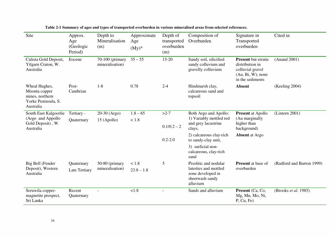
more clay rich (See Table 2-1). Their observations seem to suggest that although time

may be a significant factor that influences the formation of surface signatures, the local

climate, hydrologic regime and geology (including the depth and properties of the

transported layer) may be key drivers as well. Absolute ages for overburden(s) would be

useful in determining whether the differences encountered within such studies may be

due to small differences in the timescale.

The depth of the transported material and the formation of geochemical anomalies

within it can certainly be seen to be affected by time (Govett 1976; Hamilton 1998;

Radford and Burton 1999). Butt et al. (2000) have suggested, based on evidence from

numerous field studies, that unless the transported overburden is sufficiently shallow

(< 5 m), there will be no geochemical expression in the soils (developed from the

overburden) or in the overburden. In contrast, geochemical signatures in transported

overburden have been found at thicknesses of ~20-30 m with the ages of the overburden

in these cases being significantly older (Anand et al. 2001) (Tertiary, in contrast to the

Quaternary materials reported in Butt et al. (2000) and Sahoo and Pandalai (2000).

However, there are still insufficient data to assess whether a relationship exists between

the depth of the transported overburden and the presence of geochemical signatures.

Similarly, the lack of research with respect to the rate of trace element uptake at depth,

turnover and loss within undisturbed terrestrial ecosystems has meant that little can be

inferred about the rate of plant uptake within an ecosystem over a mineralised zone. In

view of that, there is a considerable need for the development of models that account for

the effect of time on the formation of soil geochemical anomalies by biological agents,

or by any upward migration mechanism. An approximation for this time value may be

13

obtained from the ages of transported overburden and the development of signatures

within it, if it is assumed that vegetation has been productively growing on the

overburden (Table 2-1). The review of the literature seems to suggest that soil

anomalies generally take upwards of ~1 × 106 years to form in transported overburden

(assuming that ages of overburden indicate the upper limit of the approximate time

taken to accumulate ore elements in the surface and from cases of no signal in the

surface soil of transported overburden (eg. Keeling 2004) (Table 2-1)).

In addition, the discussion in the previous sections suggests that depth to mineralisation

(or to a residual signature in older regolith) will affect the net biogenic uptake of

elements into the upper regolith profile. This effect may be apparent if the depth to

mineralisation is sufficiently large, such that it is beyond the reach of plant roots.

Hence, an initial mechanism in which a dispersion halo around the ore deposit is already

present, due to dispersion mechanisms such as hydromorphic dispersion, brings ore

elements within reach of the rooting depth. Some data seem to suggest that at great

depths to mineralisation (eg., 400 m depth to mineralisation from Anand et al. (2004),

vertical migration into the topmost part of the regolith is limited to the base of the

overburden. In this case, vertical transport of elements by biogenic mechanisms may not

be as significant as physico-chemical processes.

2.3. Aspects of trace element biogeochemical cycling involving plants

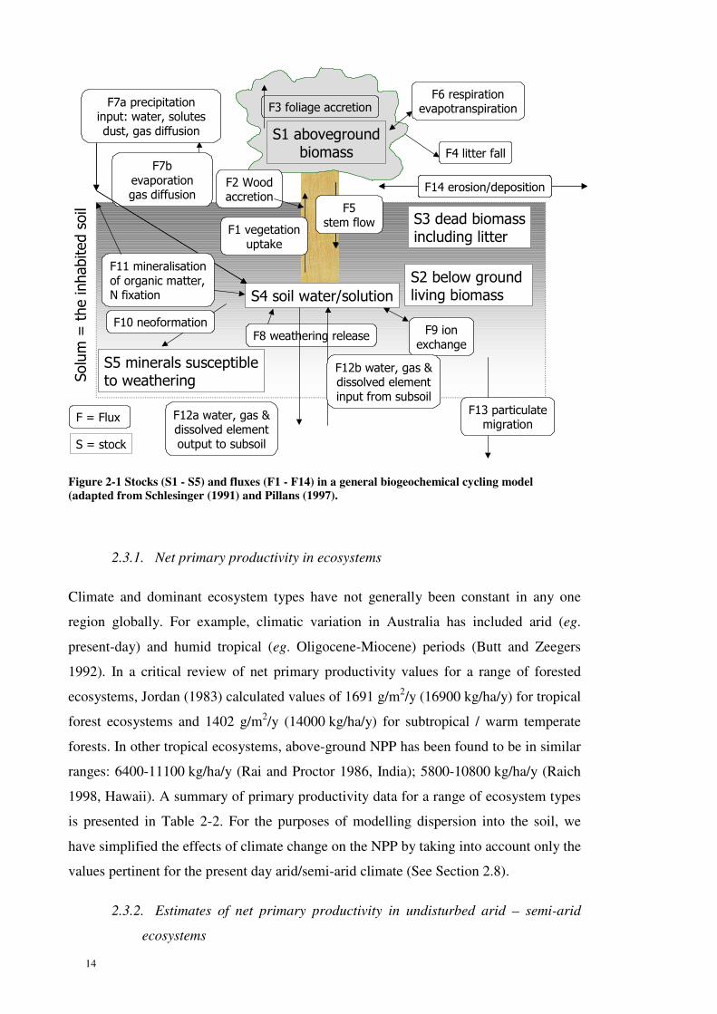
Schlesinger (1991) reviewed biogeochemical cycling in terrestrial ecosystems which is

summarised in Figure 2-1. Trace element redistribution from depth into surficial

materials by plants will be driven by several factors. Foremost are the concentrations of

trace elements in plant tissues and the productivity, in terms of biomass, of the plants;

these factors in turn are driven by climatic variables, and plant physiological attributes

such as rooting depth.

14

Solu

m =

the inhabited s

oil

S4 soil water/solution

S3 dead biomassincluding litter

S2 below ground living biomass

S5 minerals susceptibleto weathering

S1 abovegroundbiomass

F7b evaporationgas diffusion

F7a precipitationinput: water, solutesdust, gas diffusion

F2 Woodaccretion

F3 foliage accretionF6 respiration

evapotranspiration

F4 litter fall

F14 erosion/depositionF14 erosion/deposition

F5stem flow

F1 vegetationuptake

F11 mineralisationof organic matter,N fixation

F10 neoformationF8 weathering release F9 ion

exchange

F12b water, gas &dissolved elementinput from subsoil

F12a water, gas &dissolved elementoutput to subsoil

F13 particulatemigration

F = Flux

S = stock

Figure 2-1 Stocks (S1 - S5) and fluxes (F1 - F14) in a general biogeochemical cycling model

(adapted from Schlesinger (1991) and Pillans (1997).

2.3.1. Net primary productivity in ecosystems

Climate and dominant ecosystem types have not generally been constant in any one

region globally. For example, climatic variation in Australia has included arid (eg.

present-day) and humid tropical (eg. Oligocene-Miocene) periods (Butt and Zeegers

1992). In a critical review of net primary productivity values for a range of forested

ecosystems, Jordan (1983) calculated values of 1691 g/m2/y (16900 kg/ha/y) for tropical

forest ecosystems and 1402 g/m2/y (14000 kg/ha/y) for subtropical / warm temperate

forests. In other tropical ecosystems, above-ground NPP has been found to be in similar

ranges: 6400-11100 kg/ha/y (Rai and Proctor 1986, India); 5800-10800 kg/ha/y (Raich

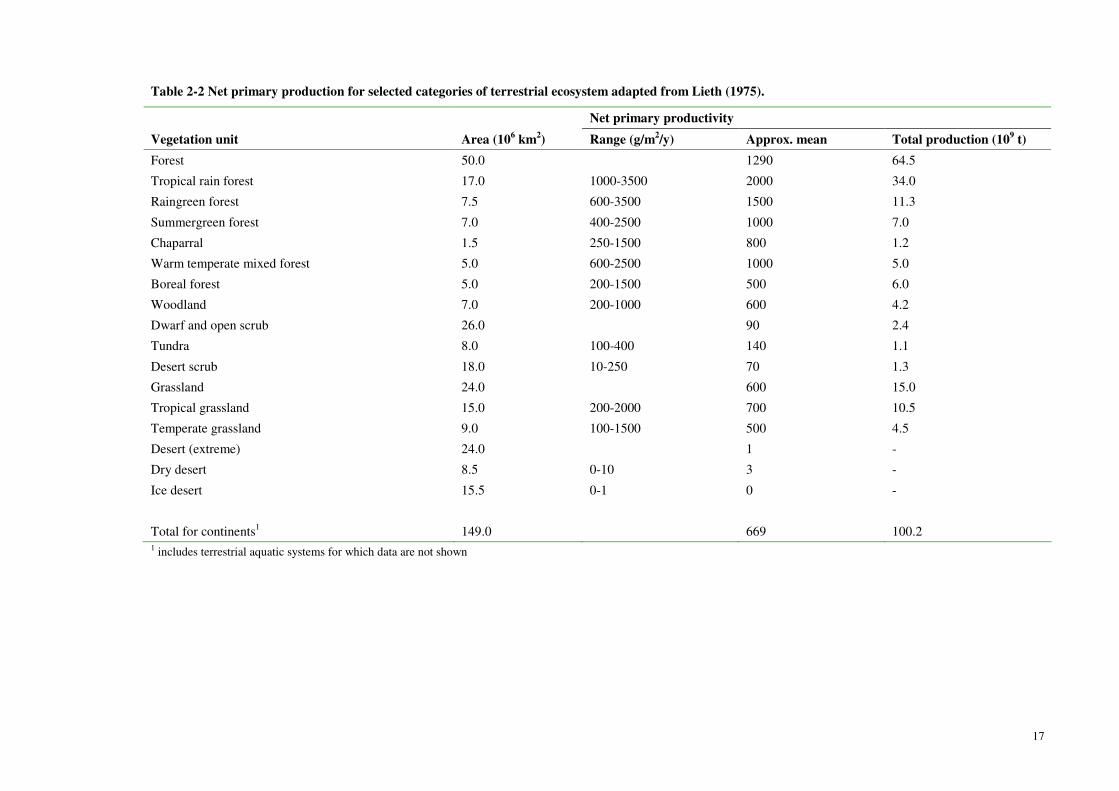
1998, Hawaii). A summary of primary productivity data for a range of ecosystem types

is presented in Table 2-2. For the purposes of modelling dispersion into the soil, we

have simplified the effects of climate change on the NPP by taking into account only the

values pertinent for the present day arid/semi-arid climate (See Section 2.8).

2.3.2. Estimates of net primary productivity in undisturbed arid – semi-arid

ecosystems

15

Published estimates of biomass production by plants in undisturbed arid - semi-arid

ecosystems are surprisingly rare in the ecological literature; most attention has been

given to managed ecosystems such as forests and agriculture. Arid and semi-arid

ecosystems in Australia generally have net primary production (NPP) values of 400 –

2400 kg/ha/y of dry matter (= 40-240 g/m2/y); grasslands in semi-arid USA have

recorded NPP values of between 1000 kg/ha/yr to 7000 kg/ha/yr (Sala et al. 1988),

while drylands in semi-arid south Africa have NPP’s ranging from 695 to 2300 kg/ha/yr

(Synman 2005). A ‘typical’ global estimate for a semi-arid ecosystem would be 150

g/m2/y (1500 kg/ha/y) (Table 2-2). In compiling the data, it has been assumed that

biomass production in natural, undisturbed ecosystems can be estimated directly from

plant tissue production, litter fall, or mineralisation of soil organic matter since over

geological time scales these fluxes should all be equal in steady-state ecosystems.

Similarly, for the purposes of trace element biogeochemical cycling, it is likely to be

unimportant whether organic matter is mineralised by biological process or by fire,

except for volatile elements such as mercury. Since only contemporary estimates of

ecosystem productivity are available, subsequent mass balance calculations most

conveniently assume that biomass production by plants has been effectively constant

over geological time scales.

2.3.3. Plant uptake of trace elements

There are more than sufficient data demonstrating that plants can accumulate trace

elements which are of importance economically or for exploration purposes. Several

trace elements (B, Co, Cu, Mn, Mo, Zn) are essential for the physiological functioning

of plants (Kabata-Pendias and Pendias 1992; Pais and Jones 1997; Reuter and Robinson

1997). Considerable data on trace element contents of plant tissues are available from

studies which focus on the ability of plants to express surface geochemical anomalies in

mineralised areas (Dunn 1986; Valente et al. 1986; Reading et al. 1987; Rogers and

Dunn 1993; McInnes et al. 1996; Lintern et al. 1997; Noller et al. 1997; Cohen et al.

1998a; Lintern and Butt 1998; Lintern 1999). Plant uptake may also be influenced by

the plant species — different species may accumulate different elements and different

plant parts will accumulate different elements (Dunn and Ray 1995; Brooks 1998).

16

Table 2-1 Summary of ages and types of transported overburden in various mineralised areas from selected references.

Site Approx.

Age

(Geologic

Period)

Depth to

Mineralisation

(m)

Approximate

Age

(My)*

Depth of

transported

overburden

(m)

Composition of

Overburden

Signature in

Transported

overburden

Cited in

Calista Gold Deposit,

Yilgarn Craton, W.

Australia

Eocene 70-100 (primary

mineralisation)

35 – 55 15-20 Sandy soil, silicified

sandy colluvium and

gravelly colluvium

Present but erratic

distribution in

colluvial gravel

(Au, Bi, W); none

in the sediments

(Anand 2001)

Wheal Hughes,

Moonta copper

mines, northern

Yorke Peninsula, S.

Australia

Post-

Cambrian

1-8 0.78 2-4 Hindmarsh clay,

calcareous sand and

topsoil

Absent (Keeling 2004)

South East Kalgoorlie

(Argo and Appollo

Gold Deposit) , W.

Australia

Tertiary -

Quaternary

20-30 (Argo)

15 (Apollo)

1.8 – 65

< 1.8

>2-7

0.1/0.2 – 2

0.2-2.0

Both Argo and Apollo:

1) Variably mottled red

and grey lacustrine

clays,

2) calcareous clay-rich

to sandy-clay unit,

3) surficial non-

calcareous, clay-rich

sand

Present at Apollo

(Au marginally

higher than

background)

Absent at Argo

(Lintern 2001)

Big Bell (Fender

Deposit), Western

Australia

Quaternary

Late Tertiary

50-80 (primary

mineralisation)

< 1.8

23.8 – 1.8

5 Pisolitic and nodular

laterites and mottled

zone developed in

sheetwash sandy

alluvium

Present at base of

overburden

(Radford and Burton 1999)

Seruwila copper-

magnetite prospect,

Sri Lanka

Recent

Quaternary

- <1.8 - Sands and alluvium Present (Ca, Co,

Mg, Mn, Mo, Ni,

P, Cu, Fe)

(Brooks et al. 1985)

17

Table 2-2 Net primary production for selected categories of terrestrial ecosystem adapted from Lieth (1975).

Net primary productivity

Vegetation unit Area (106 km

2) Range (g/m

2/y) Approx. mean Total production (10

9 t)

Forest 50.0 1290 64.5

Tropical rain forest 17.0 1000-3500 2000 34.0

Raingreen forest 7.5 600-3500 1500 11.3

Summergreen forest 7.0 400-2500 1000 7.0

Chaparral 1.5 250-1500 800 1.2

Warm temperate mixed forest 5.0 600-2500 1000 5.0

Boreal forest 5.0 200-1500 500 6.0

Woodland 7.0 200-1000 600 4.2

Dwarf and open scrub 26.0 90 2.4

Tundra 8.0 100-400 140 1.1

Desert scrub 18.0 10-250 70 1.3

Grassland 24.0 600 15.0

Tropical grassland 15.0 200-2000 700 10.5

Temperate grassland 9.0 100-1500 500 4.5

Desert (extreme) 24.0 1 -

Dry desert 8.5 0-10 3 -

Ice desert

15.5 0-1 0 -

Total for continents1 149.0 669 100.2

1 includes terrestrial aquatic systems for which data are not shown

18

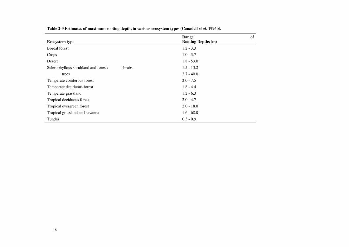
Table 2-3 Estimates of maximum rooting depth, in various ecosystem types (Canadell et al. 1996b).

Ecosystem type

Range of

Rooting Depths (m)

Boreal forest 1.2 - 3.3

Crops 1.0 - 3.7

Desert 1.8 - 53.0

Sclerophyllous shrubland and forest: shrubs 1.5 - 13.2

trees 2.7 - 40.0

Temperate coniferous forest 2.0 - 7.5

Temperate deciduous forest 1.8 - 4.4

Temperate grassland 1.2 - 6.3

Tropical deciduous forest 2.0 - 4.7

Tropical evergreen forest 2.0 - 18.0

Tropical grassland and savanna 1.6 - 68.0

Tundra 0.3 - 0.9

19

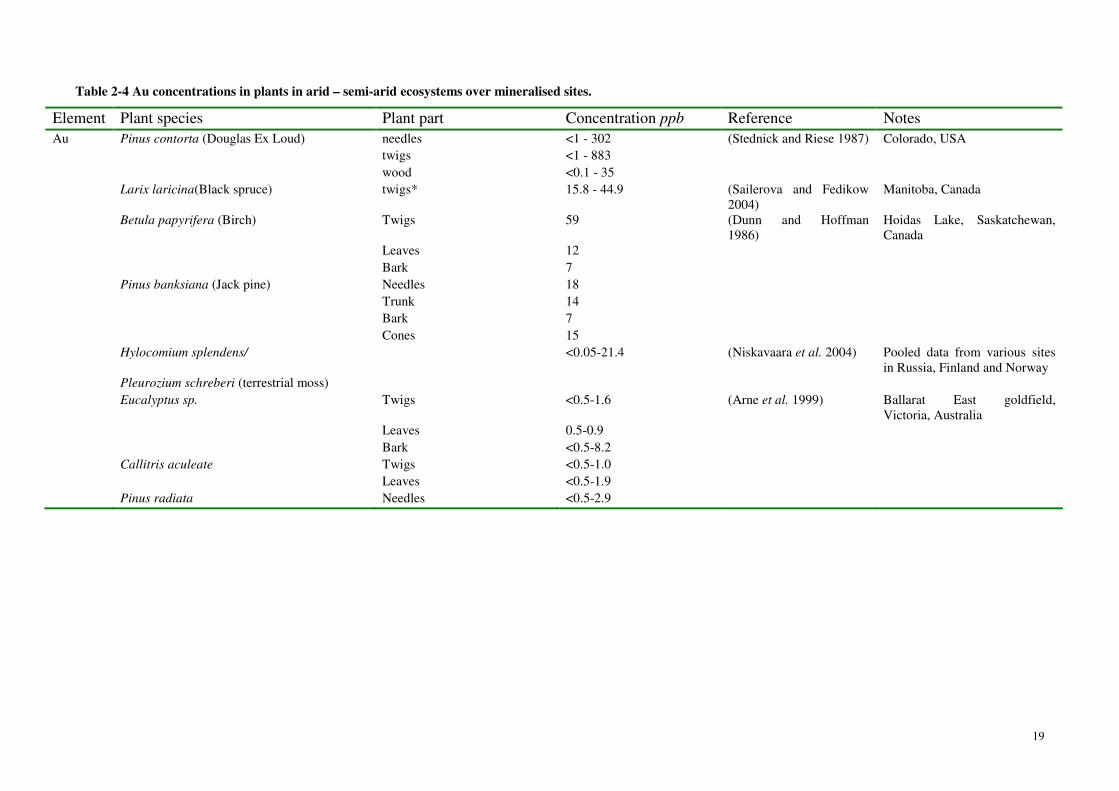
Table 2-4 Au concentrations in plants in arid – semi-arid ecosystems over mineralised sites.

Element Plant species Plant part Concentration ppb Reference Notes

Au Pinus contorta (Douglas Ex Loud) needles <1 - 302 (Stednick and Riese 1987) Colorado, USA

twigs <1 - 883

wood <0.1 - 35

Larix laricina(Black spruce) twigs* 15.8 - 44.9 (Sailerova and Fedikow

2004)

Manitoba, Canada

Betula papyrifera (Birch) Twigs 59 (Dunn and Hoffman

1986)

Hoidas Lake, Saskatchewan,

Canada

Leaves 12

Bark 7

Pinus banksiana (Jack pine) Needles 18

Trunk 14

Bark 7

Cones 15

Hylocomium splendens/ <0.05-21.4 (Niskavaara et al. 2004) Pooled data from various sites

in Russia, Finland and Norway

Pleurozium schreberi (terrestrial moss)

Eucalyptus sp. Twigs <0.5-1.6 (Arne et al. 1999) Ballarat East goldfield,

Victoria, Australia

Leaves 0.5-0.9

Bark <0.5-8.2

Callitris aculeate Twigs <0.5-1.0

Leaves <0.5-1.9

Pinus radiata Needles <0.5-2.9

20

Table 2-5 As concentrations in plants in arid – semi-arid ecosystems over mineralised sites

Element Plant species Plant part Concentration ppm Reference Notes

As Eucalyptus sp. Twigs 0.10-0.92 (Arne et al. 1999) Ballarat East goldfield, Victoria,

Australia

Leaves 0.10-0.54

Bark 0.10-0.60

Callitris aculeate Twigs <0.05-0.38

Leaves

Pinus radiata Needles <0.05-0.57

Betula papyrifera (Birch) Twigs 1.1 (Dunn and Hoffman

1986)

Hoidas Lake, Saskatchewan, Canada

Leaves 0.8

Bark 1

Pinus banksiana (Jack pine) Needles 0.9

Trunk <0.7

Bark <0.4

Cones 7.4

21

Table 2-6 Cu concentrations in plants in arid – semi-arid ecosystems over mineralised sites


Cu Rhodendon ponticum composite of twigs and leaves 5 - 25 (Ackay et al. 1998) Turkey

Rhodendon luteum composite of twigs and leaves 1 - 50

Corylus avellana composite of twigs and leaves 4 - 23

Cistus ladinifer (Neves Corvo area; Cu, Sn

and Pb mineralisation)

leaves 64.4 - 591.5 (Batista et al. 2007) Portugal

roots 9.1 - 176

Cistus ladinifer (Brancanes area; Cu

mineralisation)

leaves 7.1 - 10.9

roots 2.8 - 9.1

Cistus ladinifer (over old mines; Cu and Mn

mineralisation)

leaves 22.6 - 98

roots 4.5 - 8.7

Pinus contorta (Douglas Ex Loud) needles 21 - 191 (Stednick and Riese 1987) Colorado, USA

twigs 56 - 1154

wood <0.5 - 13.0

Larix laricina(Black spruce) twigs* 152 - 225 (Sailerova and Fedikow

2004)

Manitoba, Canada

22

Table 2-7 Pb concentrations in plants in arid – semi-arid ecosystems over mineralised sites


Pb Rhodendon ponticum composite of twigs and leaves 5 - 1244 (Ackay et al. 1998) Turkey






roots 0.6 - 3.5


mineralisation)

leaves 0.6 - 0.8

roots 0.2 - 1.6


mineralisation)

leaves 1.1 - 4.5

roots 0.7 - 7


twigs 52 - 450

wood -

Larix laricina(Black spruce) twigs* 6.25 - 17.9 (Sailerova and Fedikow

2004)

Manitoba, Canada

23

Table 2-8 Zn concentrations in plants in arid – semi-arid ecosystems over mineralised sites


Zn Rhodendon ponticum composite of twigs and leaves 10 - 138 (Ackay et al. 1998) Turkey





leaves 54.4 - 177 (Batista et al. 2007) Portugal

roots 13.8 - 70.7


mineralisation)

leaves 12 - 19.8

roots 3 - 13


mineralisation)

leaves 60.4 - 154.5

roots 11.6 - 29.8


twigs 14 - 7420

wood 3 - 55

Larix laricina (Black spruce) twigs* 1580 - 2316 (Sailerova and Fedikow

2004)

Manitoba, Canada

Table 2-9 Fe concentrations in plants in arid – semi-arid ecosystems over mineralised sites


Fe Cistus ladinifer (Neves Corvo area; Cu, Sn



roots 382.5 - 1086.7


mineralisation)

leaves 351 - 969

roots 216 - 1745.8


mineralisation)

leaves 313.2 - 1800

roots 288.5 - 2832.9

Larix laricina (Black spruce) twigs* 0.31 % - 0.49 % (Sailerova and Fedikow

2004)

Manitoba, Canada

24

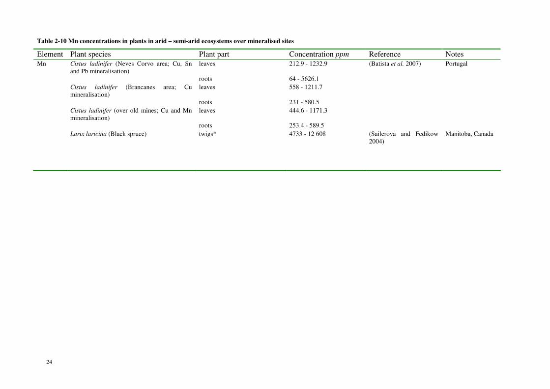
Table 2-10 Mn concentrations in plants in arid – semi-arid ecosystems over mineralised sites


Mn Cistus ladinifer (Neves Corvo area; Cu, Sn



roots 64 - 5626.1


mineralisation)

leaves 558 - 1211.7

roots 231 - 580.5


mineralisation)

leaves 444.6 - 1171.3

roots 253.4 - 589.5

Larix laricina (Black spruce) twigs* 4733 - 12 608 (Sailerova and Fedikow

2004)

Manitoba, Canada

25

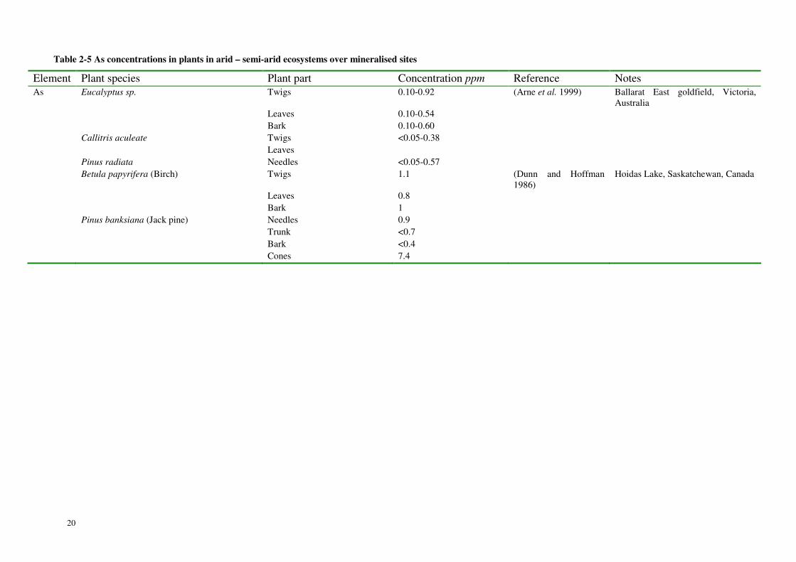
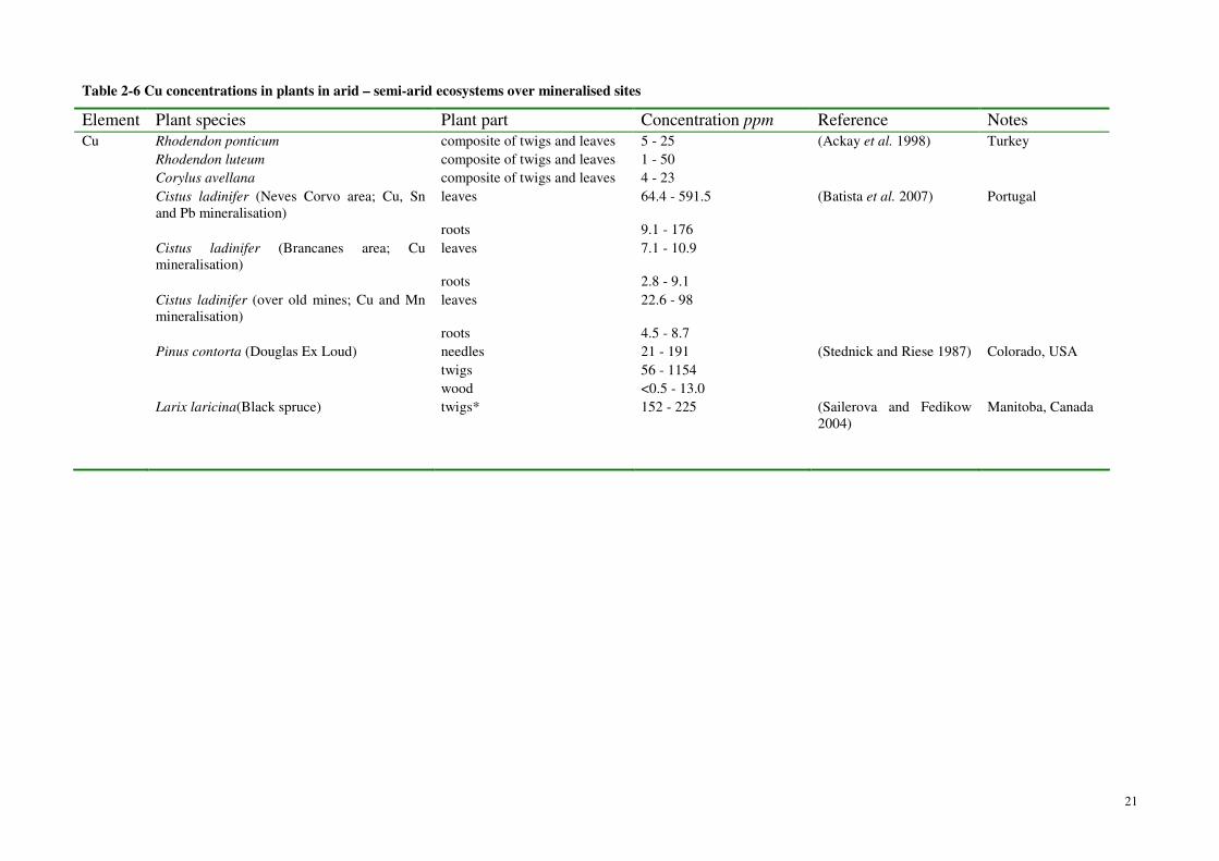
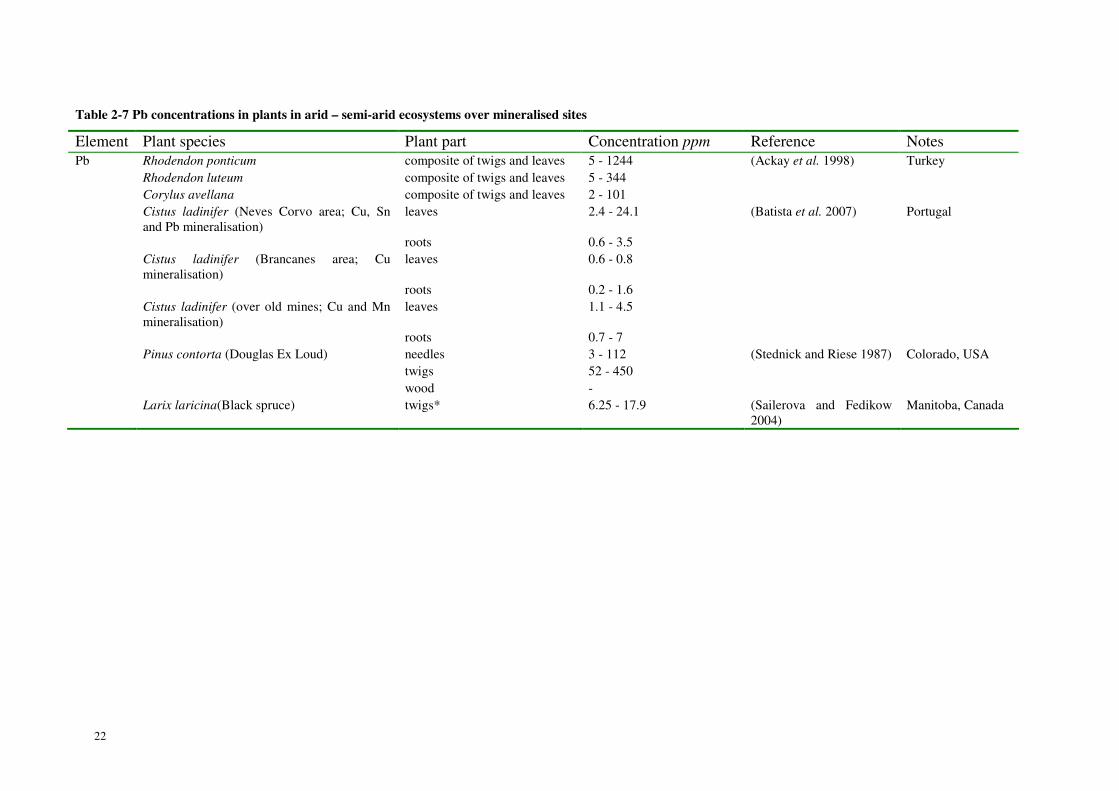
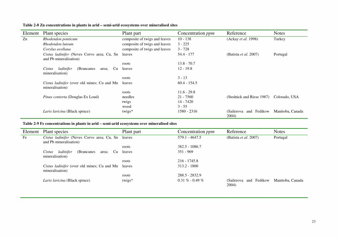
2.3.4. Trace element concentrations in plant tissues in undisturbed arid -

semi-arid ecosystems

Trace element concentrations in native vegetation in mineralised/highly polluted areas

in are remarkably variable; summaries of published data are given for Au in Table 2-4

and for As, Cu, Pb, Zn, Fe and Mn in Table 2-5 –Table 2-10. Few data for background

concentrations of trace elements in plant tissues are published, possibly because most

research has focused on exploration in mineralised areas.

2.3.5. Rooting depth of plants

The degree to which plants can absorb trace elements derived from mineralisation,

particularly in deeply weathered regolith, will be controlled to a large and unquantified

extent by the depth of plant roots. (Rooting depth will also control to a large extent the

amount of water, and therefore trace elements, moving through soil to groundwater, as

discussed below in the section ‘Leaching losses of trace elements’). The following data

(Table 2-3) are derived from a comprehensive review (Canadell et al. 1996a) of rooting

depth in a wide range of ecosystem types worldwide. The proportion of net element

uptake from deeper within the soil profile (at depths of greater than 1 m, i.e. beyond the

surface soil layer), relative to elements recycled from surface soil, remains largely

unknown. More recent work by Schenck and Jackson and co-workers (Schenk and

Jackson 2002; Schenk and Jackson 2005) has, however, suggested a dependence of deep

rooting behaviour in plants on evaporative demand with deep roots more likely to occur

in subtropical- and tropical semi-arid to humid environments which experienced

seasonal droughts. The deep uptake flux may thus be linked to the uptake of water from

groundwater sources with approximately 5 % of the total root biomass sourcing water

from depths greater than 2 m (Schenk and Jackson 2002). The use of groundwater in dry

seasons and surface soil water during the wet seaons by deep-rooted plants has been

documented in semi-arid environments by Pate et al. (1998) in south-western Australia

and Chimner and Cooper (2004) in Colorado, USA. Schenk and Jackson (2005) found

that the probability of deep rooting behaviour in plants, globally, correlates with the

aboveground plant size, with shrubs and trees four to six times more likely to root to

greater than 4 m depths. At such rooting depths, the case can be made for plant uplift in

depositional areas.

2.3.6. Production of metal-complexing ligands by plants

26

Uptake of trace elements by plants is facilitated by production of ligands by plant roots

(Römheld 1991). Soluble complexes of these ligands and metal ions increase soil

solution metal concentrations, and the complexes are able to be assimilated by plants.

One such ligand produced by plant tissues (possibly to discourage consumption by

herbivores) is cyanide (CN-), which forms stable and soluble complexes with a wide

range of metallic cations, including Au (Milligan and Muhtadi 1988; Wang and

Forssberg 1990). For example, the genera Acacia, Eucalyptus, Lotus, Pteridium, and

Zieria are known to produce cyanide or its precursors (Conn et al. 1985; Foulds and

Cartwright 1985; Flynn and Southwell 1987; Maslin et al. 1988; Low and Thomson

1990). The CN- ligand would only remain in soil given sufficient water content and pH

values near or above the pKa of HCN (ca. 9.5). This casts some uncertainty on the

geochemical significance of cyanogenesis by plants. Conversely, cyanogenesis may be

important in caliche-dominated areas, where the soils are alkaline.

Other metal complexing ligands are known to be released from the roots of plants in the

semi-arid zone. Oxalate (or oxalic acid) has been found in eucalypts (Malajczuk and

Cromack 1982; O'Connell et al. 1983) and a range of other species (Silcock and Smith

1983; Jacob and Peet 1989; Ahmed et al. 2000; McKenzie et al. 2004). Citrate has been

identified in the rhizosphere of a single Banksia species (Grierson and Adams 1999),

and is likely to exist in other species. It is likely that other compounds are also produced

which have the ability to solubilise trace elements (Dakora and Phillips 2002; Bierman

et al. 2005). The ecological significance of oxalate is questionable due to the

insolubility of calcium oxalate, but it is well-established that plants release a range of

organic ligands from their roots to enhance phosphorus and trace element nutrition

(Marschner 1995).

2.3.7. Bioturbation by plants

Bioturbation by plants mixes the top soil layers (typically the litter layer and the A

horizon) and has a homogenising effect on the physical and chemical soil properties of

top soil layers (Roering et al. 2002; Nierop and Verstraten 2004; Wilkinson and

Humphreys 2005; Kaste et al. 2007). Soil mixing thus has a major role in

biogeochemical cycling in terrestrial ecosystems. Bioturbation involves both the direct

movement of soil particles by plant root growth (and tree throw) and indirectly through

creating preferential pathways in the soil mantle for transfer of particles to depth by

water (Kaste et al.). Vertical mixing rates have been calculated at 1 – 2 cm/ka for a soil

27

depth of 35 cm in Marin County, USA (Meditarranean climate, average precipitation=

800 mm) which converts to a rate of 10-20 m/Ma (Kaste et al. 2007).

2.4. Mechanisms of trace element cycling involving soil animals

Soil animals are potentially involved in trace element cycling through the physical

mixing of soil by burrowing and foraging animals, and through consumption of organic

materials which have become enriched in trace elements as a result of plant uptake from

mineralised soil. Since physical mixing is involved, less geochemically mobile elements

can be transported, and bioturbation can be an efficient transport mechanism (Dorr

1995). Alteration of soil pore-size distributions by burrowing might be considered to

have an effect on geochemical cycling via changes in shallow hydrology, but Lobry de

Bruyn and Conacher (1994b) found that macropores created by ants were only

significant under saturated soil conditions causing ponded infiltration.

The most likely animals involved in arid and semi-arid ecosystems are the burrowing

insects (ants and termites), as a result of their extensive distribution, and this section of

the review will focus on these organisms. It is possible that larger burrowing animals,

such as mammals or reptiles, may be significant in bioturbation of soils in some areas.

For example, in Western Australia the pebble-mound mouse may redistribute ca.

50 m3/ha of soil where it is locally abundant. In South Australia the hairy-nosed wombat

can redistribute ca. 100 m3/ha of soil from burrow systems which can disrupt calcrete

and are visible in LandSat images (Whitford et al. 1997).

Data reviewed in this section suggest that animals, especially termites, may be more

involved in horizontal soil redistribution than vertical. It follows that animal activity

probably has more of a role in the lateral spread of a soil anomaly than in its formation

by vertical redistribution of soil.

2.4.1. Depth of termite or ant bioturbation

In arid environments, termites may burrow to extreme depths of 60 m to obtain water

(Butt and Zeegers 1992). In isolated instances, termite galleries have been found at

depths of between 8 and 70 m (Wood and Sands 1978; Lee 1983; Coventry et al. 1988),

but such depths are considered unusual by some authors. Wood and Sands (1978)

review literature finding that termite excavations generally do not extend below 100 cm

depth, but the maximum depths of sampling for the studies reviewed were not stated.

28

Coventry et al. (1988) found the mean depth of termite activity in the Charters Towers

area of Queensland, Australia to be 20-40 cm, but that soil chemical properties were

affected by mound-building termites to a depth of at least 80 cm. Lobry de Bruyn and

Conacher (1995) found that, in Western Australia, termite excavation was

predominantly in the upper 30 cm of soil profiles, with >50% of chambers in the top

10 cm of soil. A similar finding was reported by Wang et al. (1995) in Wisconsin where

ant activity was found to be mainly restricted to the top 70 cm of soil (main

concentration of nest chambers was in the top 30 cm of soil). It is fairly well-established

that both ants and termites selectively excavate soil fractions with higher clay content

when building mounds, which may require them to access subsoils (Lee and Wood

1971; Lee 1983; Eldridge and Myers 1998; Frouz et al. 2003).

Ants may be less important than termites in terms of soil bioturbation. Abensperg-Traun

(1992) determined that ants made a small contribution to total ecosystem biomass in

Western Australia, in the order of 3-20 mg/m2. Lobry De Bruyn and Conacher (1995)

reviewed literature finding that the proportion of land surface affected by ants was ca.

0.4%, compared with up to 20% (0.27-20%) by termites, but their dataset was

incomplete in this regard. Hart (1995) also implicated ants in texture-contrast soil

formation. Ant biopores up to 60 cm deep have been observed in Western Australia

(Lobry De Bruyn and Conacher 1994b).

2.4.2. Horizontal extent of termite or ant bioturbation

Termites create feeding galleries by shallow excavation of soil around the mound or

nest site. Most observations have found these approximately horizontal burrows to

extend 20-30 m radially from nests or mounds for Australian termites (Wood and Sands

1978; Lobry De Bruyn and Conacher 1995). Whitford et al. (1992) found that an area of

ca. 137.5 m2 around termite mounds contained feeding galleries. The land surface area

affected by termite mounds and excavations at any one point in time has been estimated

in the range 0.2-20% (Lobry De Bruyn and Conacher 1990). In contrast with the wider

lateral extent of termite bioturbation, ant activity has been found to extend 0-15 cm

from the nest (Lobry De Bruyn and Conacher 1994a).

2.4.3. Amount of soil relocation from termite or ant bioturbation

The amount of soil brought to the surface by termites is dependent on species

composition and density of termite colonies in any particular ecosystem. A range of

29

estimates of soil – surface flux is listed in Table 2-14. Hart (1995) proposed that sand-

over-clay texture contrast soils may form via bioturbation by termites or ants, as the

colonies selectively excavate clay from topsoils which is then preferentially eroded

from mounds at the surface, leaving a sandy topsoil. Estimates of soil redistribution by

ants range from 0.6 – 8410 kg/ha/y, and are on average lower than estimates for termite

bioturbation (Table 2-14). The data may be confounded by the possibility that some

estimates are averaged over large land areas, whereas others (possibly at the higher end

of the scale) may represent only the area directly disturbed by insect activity.

2.5. Losses of Trace Elements from the Soil-Plant System

Accumulation of metals in the soil-plant system needs also to account for the loss of

accumulated metals, since only net accumulation will result in formation of a

biogeochemical anomaly in soil. The most important mechanisms for loss of trace

elements following accumulation in soils by biota are likely to be soil erosion by wind

and water, and loss as soluble species by leaching and/or lateral flow.

2.5.1. Leaching losses of trace elements

It is presumed that leaching losses can be estimated from metal concentrations in

groundwater in combination with estimates of deep drainage flux of water. The other

potential losses of trace elements in water would be by overland flow (runoff) and

lateral subsurface flow, but insufficient data exist to make estimates of loss fluxes by

these mechanisms sensible.

2.5.1.1. Metal concentrations in groundwater

Most measurements of trace element concentrations in groundwaters in (semi)arid

regions have been made for purposes of exploration in mineralised areas (for example,

Kelepertisis (2001) and Gray (1992)) (See Table 2-11). Clearly these are contemporary

concentration values, and may not represent concentrations of trace elements in vadose-

zone in surface soils. Any subsequent calculations of loss of trace elements to deep

groundwater are therefore very approximate.

2.5.1.2. Deep drainage (groundwater recharge)

Eastham et al. (2000) determined that net vertical water movement was generally

upwards (0-30 mm) in silvicultural areas of a semi-arid region of Western Australia

30

(annual rainfall 350 mm; pan evaporation 2302 mm). Similarly, Allison and Hughes

(1972) found no significant groundwater recharge to forested sites following canopy

closure. In agricultural systems in semi-arid zones of Australia, recharge to groundwater

is generally low (< 40 mm/y)(Allison and Hughes 1972). In general, recharge under

natural vegetation in semi-arid Australia is <1 mm/y (Dawes et al. 2002).Values for

other semi-arid areas have been calculated (using water balance), for example in Ghana,

water balance calculations for a gold mining district were calculated at between 199 –

299 mm/y (Kuma 2007). However this recharge value is larger than would be in a

natural ecosystem because their value accounts for the impact of mining activities in the

catchment. A deep drainage value was also calculated for cropped land in semi-arid

northeastern Nigeria at an average of 14 mm/y over a 36 year period (Eilers et al. 2007).

Data from several other studies (Anand and Paine 2002; Bierman et al. 2005; Jayko

2005; Wilkinson and Humphreys 2005; Kaste et al. 2007; Kober et al. 2007; Pillans

2007) suggest that recharge to groundwater lies between 0 – 100 mm/y in most semi-

arid ecosystems. For an in-depth global synthesis of groundwater recharge in arid to

semi-arid areas, please see Scanlon et al. (2006).

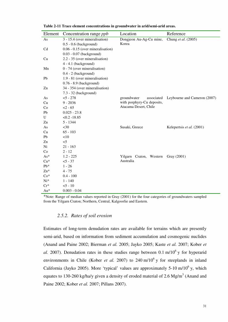
31

Table 2-11 Trace element concentrations in groundwater in arid/semi-arid areas.

Element Concentration range ppb Location Reference

As 3 - 15.4 (over mineralisation) Chung et al. (2005)

0.5 - 0.6 (background)

Dongjeon Au-Ag-Cu mine,

Korea

Cd 0.06 - 0.15 (over mineralisation)


Cu 2.2 - 35 (over mineralisation)

4 - 4.1 (background)

Mn 0 - 74 (over mineralisation)

0.4 - 2 (background)

Pb 1.9 - 81 (over mineralisation)


Zn 34 - 354 (over mineralisation)

7.3 - 32 (background)

As <5 - 278 Leybourne and Cameron (2007)

Cu 9 - 2036

Co <2 - 65

groundwater associated

with porphyry-Cu deposits,

Atacama Desert, Chile

Pb 0.025 - 23.8

U <0.2 -18.85

Zn 5 - 1344

As <30 Susaki, Greece Kelepertsis et al. (2001)

Cu 65 - 103

Pb <10

Zn <5

Ni 21 - 163

Co 2 - 12

As* 1.2 - 225 Gray (2001)

Cu* <5 - 37

Yilgarn Craton, Western

Australia

Pb* 1 - 26

Zn* 4 - 75

Co* 0.4 - 100

Ni* 1 - 140

Cr* <5 - 10

Au* 0.003 - 0.04

*Note: Range of median values reported in Gray (2001) for the four categories of groundwaters sampled

from the Yilgarn Craton; Northern, Central, Kalgoorlie and Eastern.

2.5.2. Rates of soil erosion

Estimates of long-term denudation rates are available for terrains which are presently

semi-arid, based on information from sediment accumulation and cosmogenic nuclides

(Anand and Paine 2002; Bierman et al. 2005; Jayko 2005; Kaste et al. 2007; Kober et

al. 2007). Denudation rates in these studies range between 0.1 m/106 y for hyperarid

environments in Chile (Kober et al. 2007) to 240 m/106 y for steeplands in inland

California (Jayko 2005). More ‘typical’ values are approximately 5-10 m/106 y, which

equates to 130-260 kg/ha/y given a density of eroded material of 2.6 Mg/m3 (Anand and

Paine 2002; Kober et al. 2007; Pillans 2007).

32

Very few quantitative measurements of soil erosion have been made for undisturbed

arid to semi-arid ecosystems. There are several studies which make estimates of soil

erosion in managed semi-arid ecosystems such as agricultural or silvicultural areas for

example (Harper and Gilkes 1994; Wallbrink and Murray 1996; Lopez-Bermudez et al.

1998; Chirino et al. 2006). Most erosion studies frequently assume that the erosion rates

measured are relative to undisturbed reference sites, where erosion is minimal.

Pedogenetic studies e.g. in Pillans (1997) and in Wilkinson and Humphreys (2005) also

assume minimal erosion in semi-arid environments.

Values for soil erosion are also available from studies which estimate net soil

accumulation from termite bioturbation, from the difference between observed and

calculated accumulation of apparently redistributed soil material. Wood and Sands

(1978) suggest a value of 4500 m3/ha in 12,000 y (= ca. 550 kg/ha/y, using dry bulk

density = 1.5 Mg/m3). Similarly, Coventry et al. (1988) suggest a soil erosion flux of ca.

300-400 kg/ha/y, assuming a stable landscape and a steady-state between addition of

soil to termite mounds and simultaneous soil erosion. In the absence of other data, these

estimates are possibly the most useful for undisturbed ecosystems, and agree reasonably

well with the values for long-term denudation rates above.

2.6. Abiotic Additions to the Soil-Plant System

Apart from additions of trace elements from mineralisation, for which we have already

discussed the range of mechanisms suggested, the main abiotic additions of trace

elements to soil at any locality are from deposition of sediments (alluvial, colluvial,

aeolian, etc.) and from atmospheric deposition or fallout. Of these, only atmospheric

depositional fluxes can be sensibly discussed, since the possibilities for sediment

depositional fluxes are almost infinite with respect to both type of deposit and trace

element content of the deposited material.

2.6.1. Atmospheric Fluxes

Trace elements are normally present in the air as aerosol particles (Alloway 1995).

Metals in aerosols can be transferred into the soil reservoir by either wet or dry

atmospheric deposition (Rea et al. 2001; Starr et al. 2003). Table 2-15 shows that the

deposition rates for some elements are minimal and increase with proximity to

populated areas. Atmospheric depositional fluxes into soils may be enhanced by

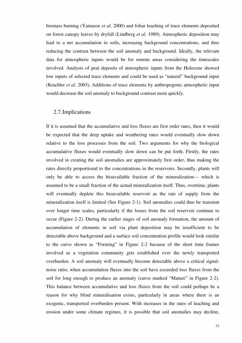
33

biomass burning (Yamasoe et al. 2000) and foliar leaching of trace elements deposited

on forest canopy leaves by dryfall (Lindberg et al. 1989). Atmospheric deposition may

lead to a net accumulation in soils, increasing background concentrations, and thus

reducing the contrast between the soil anomaly and background. Ideally, the relevant

data for atmospheric inputs would be for remote areas considering the timescales

involved. Analysis of peat deposits of atmospheric inputs from the Holocene showed

low inputs of selected trace elements and could be used as “natural” background input

(Krachler et al. 2003). Additions of trace elements by anthropogenic atmospheric input

would decrease the soil anomaly to background contrast more quickly.

2.7. Implications

If it is assumed that the accumulative and loss fluxes are first order rates, then it would

be expected that the deep uptake and weathering rates would eventually slow down

relative to the loss processes from the soil. Two arguments for why the biological

accumulative fluxes would eventually slow down can be put forth. Firstly, the rates

involved in creating the soil anomalies are approximately first order, thus making the

rates directly proportional to the concentrations in the reservoirs. Secondly, plants will

only be able to access the bioavailable fraction of the mineralization— which is

assumed to be a small fraction of the actual mineralization itself. Thus, overtime, plants

will eventually deplete this bioavailable reservoir as the rate of supply from the

mineralization itself is limited (See Figure 2-1). Soil anomalies could thus be transient

over longer time scales, particularly if the losses from the soil reservoir continue to

occur (Figure 2-2). During the earlier stages of soil anomaly formation, the amount of

accumulation of elements in soil via plant deposition may be insufficient to be

detectable above background and a surface soil concentration profile would look similar

to the curve shown as “Forming” in Figure 2-2 because of the short time frames

involved as a vegetation community gets established over the newly transported

overburden. A soil anomaly will eventually become detectable above a critical signal:

noise ratio, when accumulation fluxes into the soil have exceeded loss fluxes from the

soil for long enough to produce an anomaly (curve marked “Mature” in Figure 2-2).

This balance between accumulative and loss fluxes from the soil could perhaps be a

reason for why blind mineralisation exists, particularly in areas where there is an

exogenic, transported overburden present. With increases in the rates of leaching and

erosion under some climate regimes, it is possible that soil anomalies may decline,

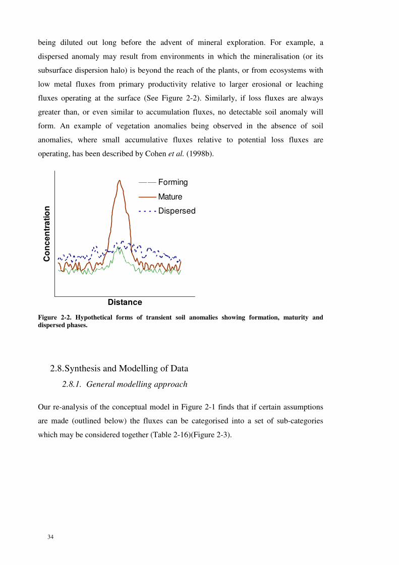
34

being diluted out long before the advent of mineral exploration. For example, a

dispersed anomaly may result from environments in which the mineralisation (or its

subsurface dispersion halo) is beyond the reach of the plants, or from ecosystems with

low metal fluxes from primary productivity relative to larger erosional or leaching

fluxes operating at the surface (See Figure 2-2). Similarly, if loss fluxes are always

greater than, or even similar to accumulation fluxes, no detectable soil anomaly will

form. An example of vegetation anomalies being observed in the absence of soil

anomalies, where small accumulative fluxes relative to potential loss fluxes are

operating, has been described by Cohen et al. (1998b).

0

0.05

0.1

0.15

0.2

0.25

0.3

0.35

0.4

0.45

0.5

-16 -6 4 14 24Distance

Co

nc

en

tra

tio

n

Forming

Mature

Dispersed

Figure 2-2. Hypothetical forms of transient soil anomalies showing formation, maturity and

dispersed phases.

2.8. Synthesis and Modelling of Data

2.8.1. General modelling approach

Our re-analysis of the conceptual model in Figure 2-1 finds that if certain assumptions

are made (outlined below) the fluxes can be categorised into a set of sub-categories

which may be considered together (Table 2-16)(Figure 2-3).

35

2.8.2. Assumptions

2.8.2.1. General assumptions

1. The flux of trace elements from buried mineralisation to the surface via cycling

through organisms is linked to the accumulation of carbon (organic matter) by the

same organisms.

2. Only net primary production (NPP) values related to the present day arid/semi-

arid climate have been used.

3. Input of organic matter (OM) by NPP is equal to the sum of OM loss by any

mechanism (mineralisation + fire + leaching + erosion + … + etc.) in a stable

ecosystem over the long term.

4. Loss fluxes of OM such as mineralisation (decomposition to CO2), stem flow

and fire (unless ash is lost outside an anomalous halo by wind action) serve to

concentrate associated non-volatile trace elements in soil. Loss fluxes of OM such

as erosion, and some leaching, serve to remove trace elements from mineralised

areas.

5. The flux of OM and associated trace elements from living to non-living soil OM

in the same ecosystem (litter fall, plant death, fire etc.) is also equal in the long term

to net primary production.

6. Animals, whether herbivorous, carnivorous or detritivorous (including soil

animals such as termites) depend on primary production for carbon/energy and do

not therefore contribute to accumulation of OM. They are, however, important in

redistributing OM.

7. The rate of rock weathering is unimportant unless it is of the same order of

magnitude as, or less than, the rate of trace element uptake calculated from NPP and

trace element content.

8. Plant rooting depth is sufficient to reach anomalous concentrations of trace

elements in deeper regolith (a reasonable expectation, given the maximum rooting

depths in Table 2-3).

36

2.8.2.2. Simplifications for mass balance calculations

1. The depth of excavation by termites and other burrowing animals,

although exceptionally to great depth, is usually <1m and therefore too shallow

for significant upward redistribution of geochemically enriched material.

2. The trace element uptake flux (U) is estimated from the annual NPP

multiplied by the trace element content of plants.

3. The loss of trace elements by soil erosion (E) is estimated from a value

for annual soil loss and a typical concentration of trace element in soil.

4. The leaching loss of trace elements (L) is estimated from annual drainage

multiplied by a typical element concentration in groundwater.

Net trace element accumulation flux (A) is simply A = cP·NPP – (cS· fS + cW· fW)

or A = U – (E + L) Equation 1

where A = net accumulation in the soil; L = net loss by leaching/deep drainage =

cW· fW (cW = trace element content of soil solution, fW = vertical transport flux); U =

net uptake flux by vegetation = cP·NPP (cP = trace element content of plants); E =

net loss by erosion = cS· fS (cS = trace element content of soil, fS = soil erosion flux).

5. The more positive the value of A, the more likely that formation of a soil

geochemical anomaly can occur by a biogeochemical mechanism.

Mass-balance calculations were performed using a range of NPP values in the range

500-5000 kgDM/ha/y, and soil erosion values in the range 0-2000 kg/ha/y, to

realistically bracket the values for these parameters found in the literature (see Table

2-1) and the section ‘Rates of soil erosion’ above).

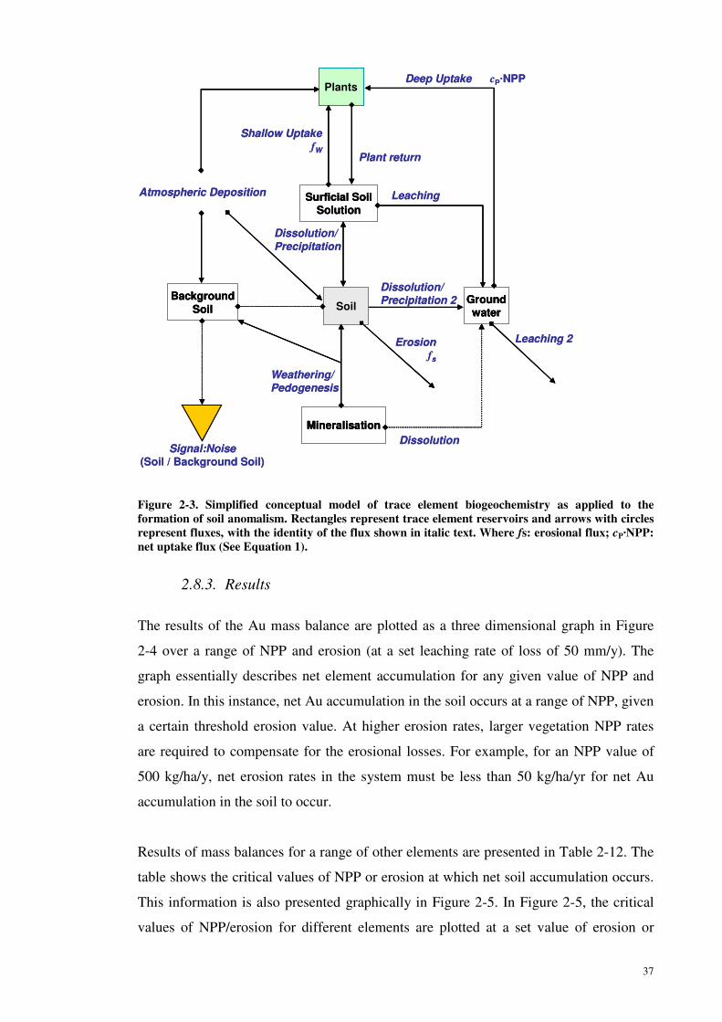
37

Deep Uptake cP·NPP

Shallow UptakefW

Atmospheric Deposition Leaching

Erosionfs

Leaching 2

DissolutionSignal:Noise

(Soil / Background Soil)

Dissolution/Precipitation 2

Dissolution/

Precipitation

Weathering/Pedogenesis

Plant return

Plants

Surficial Soil Solution

SoilGround water

Background

Soil

Mineralisation

Deep Uptake cP·NPP

Shallow UptakefW

Atmospheric Deposition Leaching

Erosionfs

Leaching 2

DissolutionSignal:Noise

(Soil / Background Soil)

Dissolution/Precipitation 2

Dissolution/

Precipitation

Weathering/Pedogenesis

Plant return

Plants


SoilGround water

Background

Soil

Mineralisation

Plants


SoilGround water

Background

Soil

Mineralisation

Figure 2-3. Simplified conceptual model of trace element biogeochemistry as applied to the

formation of soil anomalism. Rectangles represent trace element reservoirs and arrows with circles

represent fluxes, with the identity of the flux shown in italic text. Where fs: erosional flux; cP·NPP:

net uptake flux (See Equation 1).

2.8.3. Results

The results of the Au mass balance are plotted as a three dimensional graph in Figure

2-4 over a range of NPP and erosion (at a set leaching rate of loss of 50 mm/y). The

graph essentially describes net element accumulation for any given value of NPP and

erosion. In this instance, net Au accumulation in the soil occurs at a range of NPP, given

a certain threshold erosion value. At higher erosion rates, larger vegetation NPP rates

are required to compensate for the erosional losses. For example, for an NPP value of

500 kg/ha/y, net erosion rates in the system must be less than 50 kg/ha/yr for net Au

accumulation in the soil to occur.

Results of mass balances for a range of other elements are presented in Table 2-12. The

table shows the critical values of NPP or erosion at which net soil accumulation occurs.

This information is also presented graphically in Figure 2-5. In Figure 2-5, the critical

values of NPP/erosion for different elements are plotted at a set value of erosion or

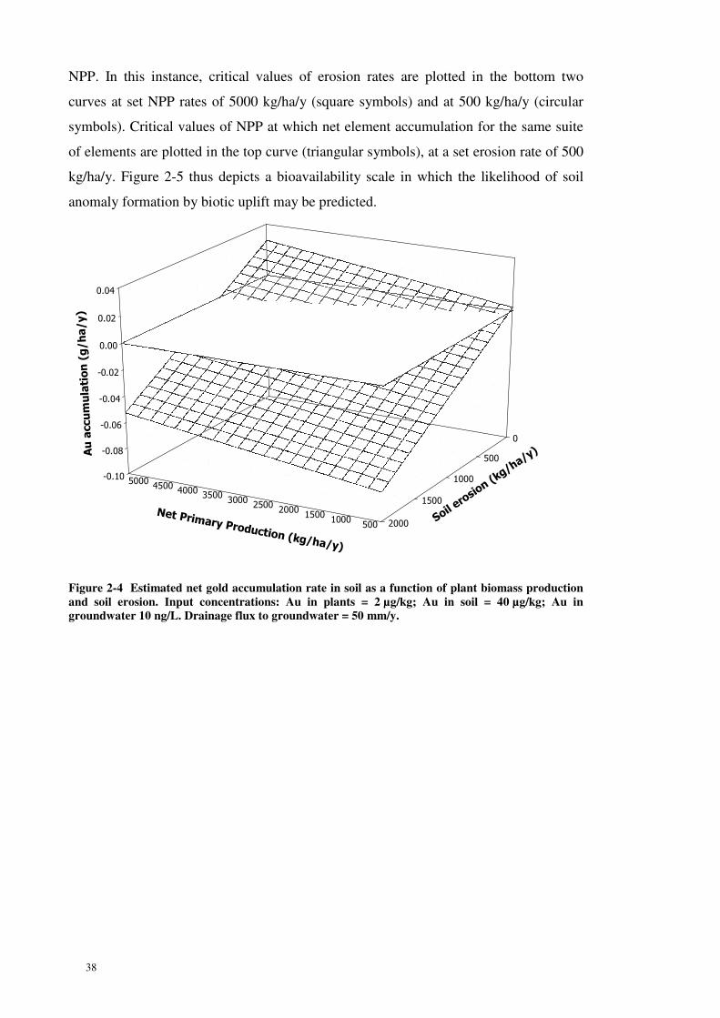
38

NPP. In this instance, critical values of erosion rates are plotted in the bottom two

curves at set NPP rates of 5000 kg/ha/y (square symbols) and at 500 kg/ha/y (circular

symbols). Critical values of NPP at which net element accumulation for the same suite

of elements are plotted in the top curve (triangular symbols), at a set erosion rate of 500

kg/ha/y. Figure 2-5 thus depicts a bioavailability scale in which the likelihood of soil

anomaly formation by biotic uplift may be predicted.

-0.10

-0.08

-0.06

-0.04

-0.02

0.00

0.02

0.04

5001000

15002000

25003000

35004000

45005000

0

500

1000

1500

2000

Au accumulation (g/ha/y)

Net Primary Production (kg/ha/y)

Soil erosion (kg/ha/y)

Figure 2-4 Estimated net gold accumulation rate in soil as a function of plant biomass production

and soil erosion. Input concentrations: Au in plants = 2 µg/kg; Au in soil = 40 µg/kg; Au in

groundwater 10 ng/L. Drainage flux to groundwater = 50 mm/y.

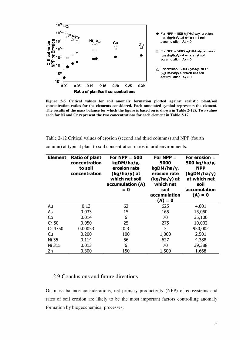
39

Figure 2-5 Critical values for soil anomaly formation plotted against realistic plant/soil

concentration ratios for the elements considered. Each annotated symbol represents the element.

The results of the mass balance for which the figure is based on is shown in Table 2-12). Two values

each for Ni and Cr represent the two concentrations for each element in Table 2-17.

Table 2-12 Critical values of erosion (second and third columns) and NPP (fourth

column) at typical plant to soil concentration ratios in arid environments.

Element Ratio of plant concentration

to soil concentration

For NPP = 500 kgDM/ha/y, erosion rate (kg/ha/y) at which net soil

accumulation (A) = 0

For NPP = 5000

kgDM/ha/y, erosion rate (kg/ha/y) at which net

soil accumulation

(A) = 0

For erosion = 500 kg/ha/y,

NPP (kgDM/ha/y) at which net

soil accumulation

(A) = 0

Au 0.13 62 625 4,001

As 0.033 15 165 15,050

Co 0.014 6 70 35,100

Cr 50 0.050 25 275 10,002

Cr 4750 0.00053 0.3 3 950,002

Cu 0.200 100 1,000 2,501

Ni 35 0.114 56 627 4,388

Ni 315 0.013 6 70 39,388

Zn 0.300 150 1,500 1,668

2.9. Conclusions and future directions

On mass balance considerations, net primary productivity (NPP) of ecosystems and

rates of soil erosion are likely to be the most important factors controlling anomaly

formation by biogeochemical processes:

40

(i) With realistic estimates of NPP and soil erosion fluxes, mass balance calculations

showed that the likelihood of anomaly formation by biotic uplift decreased in the

order Zn>Cu>Au>Ni>Cr>As>Co for Ni/Cr-poor (felsic) soil environments (Figure

2-5);

(ii)Similarly, the likelihood of anomaly formation by biotic uplift decreased in the order

Zn>Cu>Au >As>Co≈Ni>Cr for Ni/Cr-rich (mafic-ultramafic) soil environments

(Figure 2-5);

(iii)Activities of soil macrofauna (eg. termites) are not likely to affect the development

of soil anomalies per se, but may increase the rate of lateral dispersion.

Thus, Ni and Cr anomalies are unlikely to form in soil by deep biological uplift,

particularly in erosion dominated environments. On the other hand, deep biological

uplift of Zn provides relatively good anomaly contrast in the soil. The mass balance

predicts the Zn anomalies for

Although trace element budgets have been determined for a few ecosystems (Johnson

and Van Hook 1989; Kabata-Pendias and Pendias 1991), it is clear, from our discussion

in the previous chapters, that very little is known about the trace element budgets of

terrestrial ecosystems. Several conclusions can be drawn from our current review of the

literature. Firstly, it is evident that very little information is available on the amount of

trace elements held in soil solution. In addition, the following fluxes need to be

quantified: 1) net uptake from the lower horizons of the regolith by biological agents, 2)

net release back into the soil reservoir and 3) leaching and erosional losses. The

preceding discussion shows that biogeochemical cycles are complex; with many

interacting component fluxes and feedback loops (Figure 2-3). These large gaps in our

current understanding of trace element biogeochemical cycles therefore provide much

impetus for further investigation into the measurement of poorly-defined reservoirs and

fluxes, if our understanding of trace element biogeochemical cycling is to be complete.

Secondly, time is undoubtedly an important factor in determining whether surface

expression of hidden deposits occurs. The validation of a conceptual model, such as that

shown in the first part of the review, would depend on the selection of appropriate sites

if the model is to be applied in the context of how geochemical anomalies form in

transported overburdens over geological time spans. The complexity of biogeochemical

cycles means that the simple mass-balance approach that we have used is insufficient to

account for the interaction between fluxes in trace element geochemical cycles. We

41

therefore need a model that includes rate expressions to simulate the balance between

these multiple interacting fluxes. Models such as CENTURY (Parton et al. 1988), an

agroecosystem model that simulates C, N, P and S dynamics over centuries or

millennia, show an example of the level of approach needed to simulate such cycles.

The issue of identifying (and quantifying) the biological processes at work is

complicated by the many other possible translocation/accumulation mechanisms at play,

especially in ancient weathered landscapes. Selectively studying sites in which an

exogenic transported overburden is present, however, would allow elimination of some

of the other processes (such as residual enrichment) that lead to accumulation of

elements in surface soils. In addition to this, by making use of what is currently known

about the trace element biogeochemical cycle, it is possible to place further restrictions

on the selection criteria of study sites which limit the number of possible mechanisms of

dispersion. These restrictions encompass the use of current low estimates of NPP values

(for arid ecosystems), a low net uptake of elements, the presence of a transported

overburden that is at least 2 × 106 y and is sufficiently shallow (<10 m; in a stable

landscape where erosion is minimal).

Several hypotheses now emerge regarding the factors leading to the formation of

biogeochemical anomalies. Our preliminary biogeochemical calculations illustrate that

loss fluxes and accumulative fluxes must exist in an approximate steady-state, involving

excess accumulation, for soil anomalies to form. For an undisturbed ecosystem, if

accumulation of trace elements in the surface soil is to occur, the biological contribution

to the translocation of trace elements depends on a net uptake flux from deep within the

regolith to the surface soil in long-term disequilibrium with loss fluxes such as leaching

and erosion. The requirement for disequilibrium suggests that geochemical anomalies in

soils are transient features. That is, these soil anomalies form and disperse as a result of

the relative and changing sizes of the accumulative and loss fluxes. Further, using

vegetation to represent the biological component, the biological uptake flux will thus

depend on whether the vegetation is sufficiently deep-rooted to have access to the sub-

soil layers. Quantification of a deep uptake flux of any element has never been achieved

and would add great value to the body of scientific knowledge concerning plant nutrient

cycling and pedogenesis in general. In this context, the partitioning of plant water usage

between the soil water and groundwater (and hence the bioavailable trace elements in

the deeper parts of the regolith profile) may be important for net accumulation in the

surface soil to occur. This aspect of plant water uptake has only recently been studied

42

and the knowledge in this area still remains in its infancy. Finally, our initial

calculations suggest that uptake fluxes of trace elements will depend on the relative

bioavailability of each element, estimated in this work from the soil: vegetation

concentration ratio.

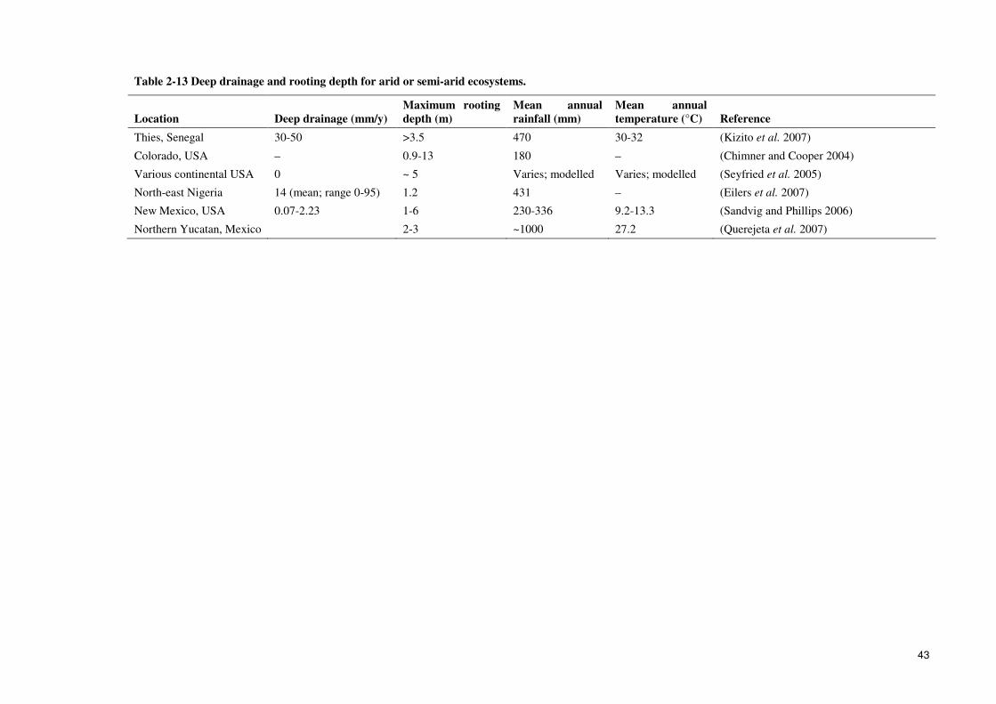
43

Table 2-13 Deep drainage and rooting depth for arid or semi-arid ecosystems.

Location Deep drainage (mm/y)

Maximum rooting

depth (m)

Mean annual

rainfall (mm)

Mean annual

temperature (°C) Reference

Thies, Senegal 30-50 >3.5 470 30-32 (Kizito et al. 2007)

Colorado, USA – 0.9-13 180 – (Chimner and Cooper 2004)

Various continental USA 0 ~ 5 Varies; modelled Varies; modelled (Seyfried et al. 2005)

North-east Nigeria 14 (mean; range 0-95) 1.2 431 – (Eilers et al. 2007)

New Mexico, USA 0.07-2.23 1-6 230-336 9.2-13.3 (Sandvig and Phillips 2006)

Northern Yucatan, Mexico 2-3 ~1000 27.2 (Querejeta et al. 2007)

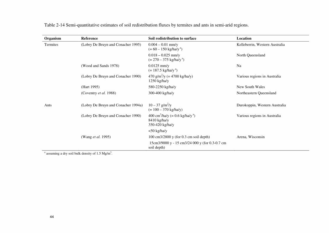
44

Table 2-14 Semi-quantitative estimates of soil redistribution fluxes by termites and ants in semi-arid regions.

Organism Reference Soil redistribution to surface Location

Termites (Lobry De Bruyn and Conacher 1995) 0.004 – 0.01 mm/y

(= 60 – 150 kg/ha/y a)

Kelleberrin, Western Australia

0.018 – 0.025 mm/y

(= 270 – 375 kg/ha/y a)

North Queensland

(Wood and Sands 1978) 0.0125 mm/y

(= 187.5 kg/ha/y a)

Na

(Lobry De Bruyn and Conacher 1990) 470 g/m2/y (= 4700 kg/ha/y)

1250 kg/ha/y

Various regions in Australia

(Hart 1995) 580-2250 kg/ha/y New South Wales

(Coventry et al. 1988) 300-400 kg/ha/y Northeastern Queensland

Ants (Lobry De Bruyn and Conacher 1994a) 10 – 37 g/m2/y

(= 100 – 370 kg/ha/y)

Durokoppin, Western Australia

(Lobry De Bruyn and Conacher 1990) 400 cm3/ha/y (= 0.6 kg/ha/y

a)

8410 kg/ha/y

350-420 kg/ha/y

<50 kg/ha/y

Various regions in Australia

(Wang et al. 1995) 100 cm3/2800 y (for 0.3 cm soil depth)

15cm3/9000 y - 15 cm3/24 000 y (for 0.3-0.7 cm

soil depth)

Arena, Wisconsin

a assuming a dry soil bulk density of 1.5 Mg/m3.

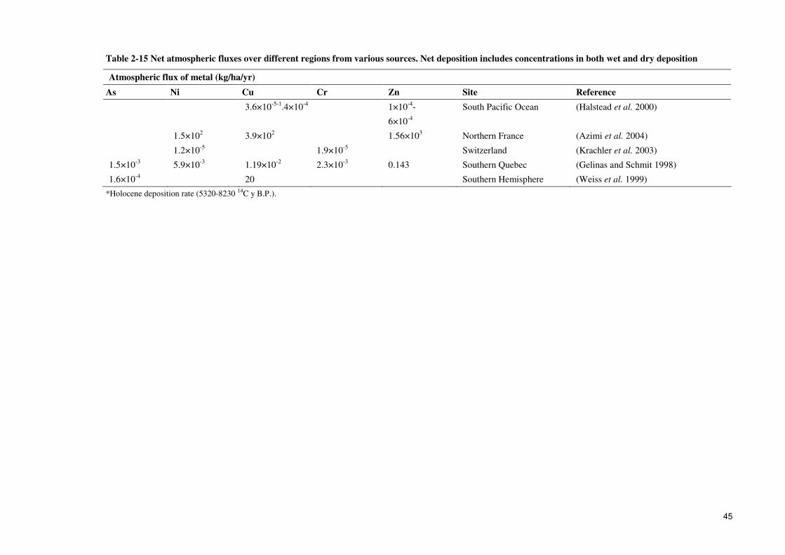
45

Table 2-15 Net atmospheric fluxes over different regions from various sources. Net deposition includes concentrations in both wet and dry deposition

Atmospheric flux of metal (kg/ha/yr)

As Ni Cu Cr Zn Site Reference

3.6×10-5-1

.4×10-4

1×10-4

-

6×10-4

South Pacific Ocean (Halstead et al. 2000)

1.5×102 3.9×10

2 1.56×10

3 Northern France (Azimi et al. 2004)

1.2×10-5

1.9×10-5

Switzerland (Krachler et al. 2003)

1.5×10-3

5.9×10-3

1.19×10-2

2.3×10-3

0.143 Southern Quebec (Gelinas and Schmit 1998)

1.6×10-4

20 Southern Hemisphere (Weiss et al. 1999)

*Holocene deposition rate (5320-8230 14C y B.P.).

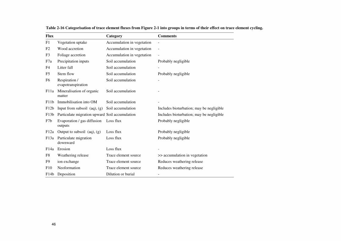
46

Table 2-16 Categorisation of trace element fluxes from Figure 2-1 into groups in terms of their effect on trace element cycling.

Flux Category Comments

F1 Vegetation uptake Accumulation in vegetation -

F2 Wood accretion Accumulation in vegetation -

F3 Foliage accretion Accumulation in vegetation -

F7a Precipitation inputs Soil accumulation Probably negligible

F4 Litter fall Soil accumulation -

F5 Stem flow Soil accumulation Probably negligible

F6 Respiration /

evapotranspiration

Soil accumulation -

F11a Mineralisation of organic

matter

Soil accumulation -

F11b Immobilisation into OM Soil accumulation -

F12b Input from subsoil (aq), (g) Soil accumulation Includes bioturbation; may be negligible

F13b Particulate migration upward Soil accumulation Includes bioturbation; may be negligible

F7b Evaporation / gas diffusion

outputs

Loss flux Probably negligible

F12a Output to subsoil (aq), (g) Loss flux Probably negligible

F13a Particulate migration

downward

Loss flux Probably negligible

F14a Erosion Loss flux -

F8 Weathering release Trace element source >> accumulation in vegetation

F9 ion exchange Trace element source Reduces weathering release

F10 Neoformation Trace element source Reduces weathering release

F14b Deposition Dilution or burial -

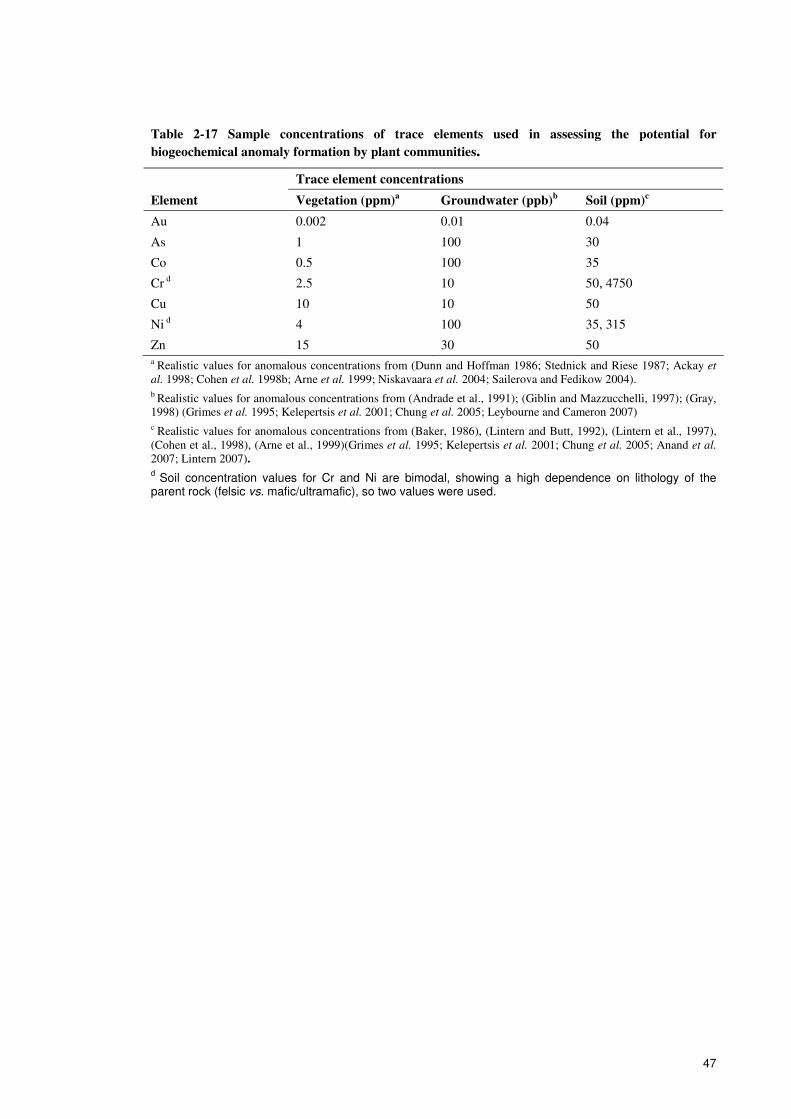
47

Table 2-17 Sample concentrations of trace elements used in assessing the potential for

biogeochemical anomaly formation by plant communities.

Trace element concentrations

Element Vegetation (ppm)a

Groundwater (ppb)b

Soil (ppm)c

Au 0.002 0.01 0.04

As 1 100 30

Co 0.5 100 35

Cr d

2.5 10 50, 4750

Cu 10 10 50

Ni d

4 100 35, 315

Zn 15 30 50 a Realistic values for anomalous concentrations from (Dunn and Hoffman 1986; Stednick and Riese 1987; Ackay et

al. 1998; Cohen et al. 1998b; Arne et al. 1999; Niskavaara et al. 2004; Sailerova and Fedikow 2004).

b Realistic values for anomalous concentrations from (Andrade et al., 1991); (Giblin and Mazzucchelli, 1997); (Gray,

1998) (Grimes et al. 1995; Kelepertsis et al. 2001; Chung et al. 2005; Leybourne and Cameron 2007)

c Realistic values for anomalous concentrations from (Baker, 1986), (Lintern and Butt, 1992), (Lintern et al., 1997),

(Cohen et al., 1998), (Arne et al., 1999)(Grimes et al. 1995; Kelepertsis et al. 2001; Chung et al. 2005; Anand et al.

2007; Lintern 2007). d

Soil concentration values for Cr and Ni are bimodal, showing a high dependence on lithology of the parent rock (felsic vs. mafic/ultramafic), so two values were used.

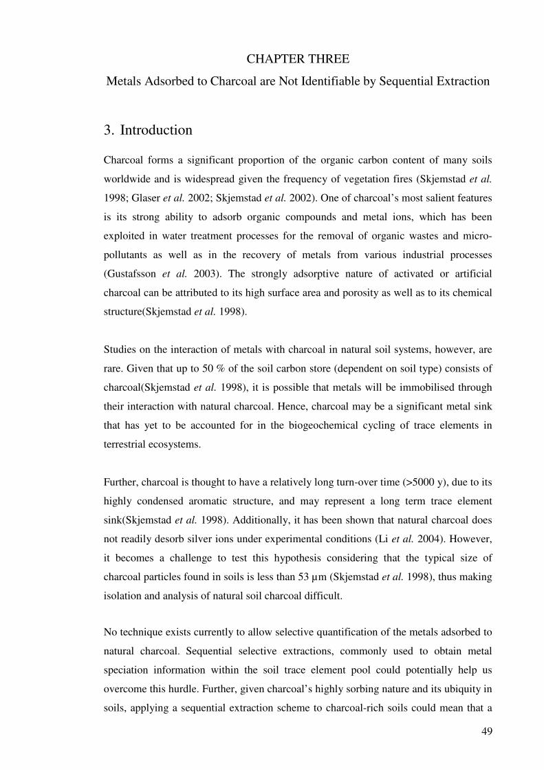
49

CHAPTER THREE

Metals Adsorbed to Charcoal are Not Identifiable by Sequential Extraction

3. Introduction

Charcoal forms a significant proportion of the organic carbon content of many soils

worldwide and is widespread given the frequency of vegetation fires (Skjemstad et al.

1998; Glaser et al. 2002; Skjemstad et al. 2002). One of charcoal’s most salient features

is its strong ability to adsorb organic compounds and metal ions, which has been

exploited in water treatment processes for the removal of organic wastes and micro-

pollutants as well as in the recovery of metals from various industrial processes

(Gustafsson et al. 2003). The strongly adsorptive nature of activated or artificial

charcoal can be attributed to its high surface area and porosity as well as to its chemical

structure(Skjemstad et al. 1998).

Studies on the interaction of metals with charcoal in natural soil systems, however, are

rare. Given that up to 50 % of the soil carbon store (dependent on soil type) consists of

charcoal(Skjemstad et al. 1998), it is possible that metals will be immobilised through

their interaction with natural charcoal. Hence, charcoal may be a significant metal sink

that has yet to be accounted for in the biogeochemical cycling of trace elements in

terrestrial ecosystems.

Further, charcoal is thought to have a relatively long turn-over time (>5000 y), due to its

highly condensed aromatic structure, and may represent a long term trace element

sink(Skjemstad et al. 1998). Additionally, it has been shown that natural charcoal does

not readily desorb silver ions under experimental conditions (Li et al. 2004). However,

it becomes a challenge to test this hypothesis considering that the typical size of

charcoal particles found in soils is less than 53 µm (Skjemstad et al. 1998), thus making

isolation and analysis of natural soil charcoal difficult.

No technique exists currently to allow selective quantification of the metals adsorbed to

natural charcoal. Sequential selective extractions, commonly used to obtain metal

speciation information within the soil trace element pool could potentially help us

overcome this hurdle. Further, given charcoal’s highly sorbing nature and its ubiquity in

soils, applying a sequential extraction scheme to charcoal-rich soils could mean that a

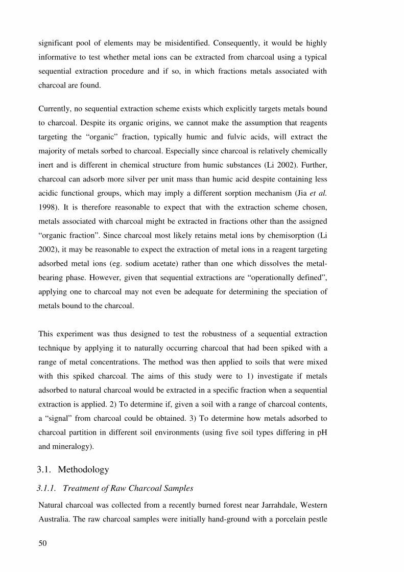
50

significant pool of elements may be misidentified. Consequently, it would be highly

informative to test whether metal ions can be extracted from charcoal using a typical

sequential extraction procedure and if so, in which fractions metals associated with

charcoal are found.

Currently, no sequential extraction scheme exists which explicitly targets metals bound

to charcoal. Despite its organic origins, we cannot make the assumption that reagents

targeting the “organic” fraction, typically humic and fulvic acids, will extract the

majority of metals sorbed to charcoal. Especially since charcoal is relatively chemically

inert and is different in chemical structure from humic substances (Li 2002). Further,

charcoal can adsorb more silver per unit mass than humic acid despite containing less

acidic functional groups, which may imply a different sorption mechanism (Jia et al.

1998). It is therefore reasonable to expect that with the extraction scheme chosen,

metals associated with charcoal might be extracted in fractions other than the assigned

“organic fraction”. Since charcoal most likely retains metal ions by chemisorption (Li

2002), it may be reasonable to expect the extraction of metal ions in a reagent targeting

adsorbed metal ions (eg. sodium acetate) rather than one which dissolves the metal-

bearing phase. However, given that sequential extractions are “operationally defined”,

applying one to charcoal may not even be adequate for determining the speciation of

metals bound to the charcoal.

This experiment was thus designed to test the robustness of a sequential extraction

technique by applying it to naturally occurring charcoal that had been spiked with a

range of metal concentrations. The method was then applied to soils that were mixed

with this spiked charcoal. The aims of this study were to 1) investigate if metals

adsorbed to natural charcoal would be extracted in a specific fraction when a sequential

extraction is applied. 2) To determine if, given a soil with a range of charcoal contents,

a “signal” from charcoal could be obtained. 3) To determine how metals adsorbed to

charcoal partition in different soil environments (using five soil types differing in pH

and mineralogy).

3.1. Methodology

3.1.1. Treatment of Raw Charcoal Samples

Natural charcoal was collected from a recently burned forest near Jarrahdale, Western

Australia. The raw charcoal samples were initially hand-ground with a porcelain pestle

51

in a porcelain mortar and sieved with a 2 mm sieve. The sieved charcoal was then

machine-ground in a grinder with a Syalon head. The ground samples were passed

through a 106 µm sieve and coarser fragments discarded. This particle size threshold for

charcoal was chosen to give a reasonable size range of charcoal particles in soil, given

that most charcoal is <53 µm in size (Skjemstad et al. 1998).

3.1.2. Cleaning of charcoal samples

The <106 µm charcoal samples were subjected to an acid-base-acid treatment (Jull et al.

1995). They were initially washed with 1M HCl to ensure the potential for interference

from any metals adsorbed to these samples was minimised. Any soluble organic matter

that may have been attached to the charcoal samples was removed by washing with 1 %

NaOH solution. The samples were then washed with 0.1 M HCl again to remove any

entrained alkali. All the charcoal samples were washed with deionised water after each

acid/base wash. The ABA treatment was carried out in acid-washed (10 % HCl) 50 mL

polypropylene centrifuge tubes. The samples were centrifuged at 4000 rpm for 5

minutes between each of the washes and the supernatants discarded.

3.2. Adsorption

3.2.1. Charcoal only experiment

The charcoal samples were treated with five different concentrations of a range of trace

metals (See Table 3-1), using five different metal stock solutions. Stock solutions were

prepared using appropriate masses of metal nitrate salts in MilliQ water. Metal stock

solution (20 mL) was added to polypropylene containers (100 mL) containing 10 g of

ABA-treated charcoal and vortexed. Sufficient amounts of 0.01 M Ca(NO3)2 solution

was added to some of the charcoal suspensions to ensure equal solution volume for all

the treatments as well as to ensure that a pH electrode could be immersed to a sufficient

solution depth. All five treatments were vortexed and the suspensions were allowed to

settle for half an hour before pH measurement. The pH of the suspensions was adjusted

to pH 6.00 (±0.03) using 6M NaOH (3 mL maximum volume added). The charcoal

suspensions were then shaken on an end-over-end shaker for 3 days at a constant

temperature of 25°C. Deionised water was included as a control. The charcoal

suspensions were vacuum filtered and dried in a 40°C oven overnight. The pH and

metal concentrations of the stock solutions and supernatants were measured as well.

52

3.2.2. Charcoal-amended soil experiment

The charcoal having the highest level of metal addition (Table 3-1) was mixed with five

different soil types to constitute 0 %, 0.25 %, 0.5 % and 1.0 % (w/w) of charcoal in 10 g

of soil. The metal concentration range was chosen to give sufficient contrast to the

background concentrations found in some of the soils that were previously characterised

by sequential extractions (Li et al. 2003). The five soils (chosen to represent typical

soils found in natural environments in Australia) that were amended with charcoal were:

1) a kaolinitic soil (Bugeye), 2) Iron oxide-rich soil (Claypan), 3) Calcareous soil

(Gala), 4) sandy soil (Ryan’s Range) and 5) lateritic sandy soil with high organic carbon

(Jarrahdale). A summary of key properties for these soils is reported in Table 3-2; the

soils cover a wide range of pH, dissolved salts, texture, organic carbon content and

mineralogy.

3.3. Sequential Extraction Procedure

The sequential extraction procedure was based on an extraction scheme developed by

Hall et al.(1996). The sequence of extractions was carried out in the order: 1) deionised

water, 2) 1.0 M Sodium acetate, pH 5 (targeting the adsorbed-exchangeable-carbonate

fraction), 3) 0.1 M sodium pyrophosphate (organic fraction), 4) 0.18 M ammonium

oxalate + 0.1 M oxalic acid; pH 3 (amorphous iron/manganese-oxides), 5) 1.0 M

hydroxylamine hydrochloride; at 90 °C in a water bath (crystalline iron/manganese

oxides) and 6) residual (1:1 aqua regia digest; 110-130 °C, digested for 1.5 hours). A

deionised water extract was included before the sodium acetate extraction step to extract

any metals that may be entrained between the charcoal particles. The aqua regia digest

was adapted for analysis of charcoal as follows: the rinsed residues from the

hydroxylamine hydrochloride extraction were ashed in a furnace at 600 °C for

approximately 12 h. The ashed charcoal samples were then digested in the ashing

crucibles with approximately 2 mL of 1:1 aqua regia on a hot plate and diluted to

10 mL for analysis by inductively-coupled plasma-mass spectrometry (ICP-MS). The

soil samples were digested in Pyrex glass digestion tubes in a block digester.

Concentrated HNO3 (2 mL) was added to each tube which was then heated at 110 ºC for

15 min. The tubes were removed and allowed to cool for 5 min before addition of

concentrated HCl. The tubes were then reheated at 110 ºC for 10 min, then at 130 ºC for

1 h. All samples were washed with 10 mL of MilliQ water between the different

extractions. Metal concentrations were also determined in wash solutions, the results of

which were included in the results for the previous, corresponding fraction.

53

3.4. Trace Metal Analysis

Trace metal analysis was carried out by flow injection-inductively-coupled plasma-mass

spectrometry (FIAS-ICP-MS) (Perkin-Elmer Elan 6000) and where Al concentrations

above the ICP-MS measurement range were encountered, by flame atomic absorption

spectrometry (Perkin-Elmer AAnalyst 300) (N2O/acetylene flame; 1000 mg/L Na+ as

ionisation-suppressant).

3.5. Quality Control

All water used was purified to a resistivity of 18.2 MΩ.cm in a Millipore ‘Milli-Q’

system. All containers and glassware were acid washed in 10 % v/v HCl. The sequential

extractions for the charcoal samples were done in triplicate. For the soil experiment,

only one concentration of charcoal was duplicated for each soil type. Each charcoal-

amended soil that was duplicated was chosen randomly. The charcoal samples were

ashed to quantitatively determine the total concentration of trace elements initially

adsorbed onto the charcoal samples. Sub-samples of charcoal (0.5 g) were placed in

porcelain crucibles and ashed at 600 °C. The samples were digested using the same

procedure as the final sequential extraction step, as described above. Reference

materials (Stream Sediment-STSD 1 (CANNMET-MMSL, Ontario, Canada), Lake

Sediment (LS-3, in-house standard) and Standard Reference Bush Leaves (GSV-2,

Institute of Geophysical and Geochemical Exploration, Hebei, China) were analysed by

the same methods. The acid digestion results for the standard reference materials (for

the elements Cr, Ni, Cu, Zn and Pb) were on average within 6 % of the reported values.

Modelling in PhreeqCi was carried out to determine whether over-saturation with

respect to any solid phases could have occurred under the given experimental conditions

3.6. Statistical Treatment

Student’s t-tests were conducted on the concentrations of metals extracted in each of the

five sequential fractions for the soil experiment. The concentrations of the control soils

from each soil type were subtracted from that of the charcoal-amended soils in each

fraction to give a comparable set of data within the different soil types, suitable for

statistical testing. The data were then tested against a null hypothesis of no change in

concentration of metals extracted in each fraction at a significance level of 0.05 by

regression analysis, using Microsoft Excel.

54

3.7. Results and Discussion

3.7.1. Sequential extraction of metals adsorbed to charcoal

The sequential extraction of charcoal for adsorbed trace metals showed reasonable

recoveries (sum of individual extraction fractions ÷ total digested from ashed charcoal)

for most metals, ranging from 80 % - 130 % with the exception of Cd (recoveries >

150 %). Therefore, Cd has been excluded from further discussion. At all concentrations

of metals added 81-100% adsorption (difference of concentrations in stock solution and

supernatant solution) was achieved for most metals except Al (21% at the lowest

concentration of metals added to charcoal) (See Table 3-3).

Lower concentrations of metals were extracted in sodium pyrophosphate, the reagent

targeting organic complexes, compared with the other reagents (Figure 3-1 and Figure

3-2). This was observed for all concentrations of metals added to the charcoal. The

metals (except Al) can be grouped into two main categories based on the fractionation

observed. Cu, Ni, Pb and Zn that display a similar trend in which most of the metals

were extracted in sodium acetate and/or ammonium oxalate, at low concentrations of

metals adsorbed (Concentration 1-4; refer to Figure 3-2). Ag and Cr make up the second

group. These metal cations display a trend in which the majority of metals (at low

adsorption concentrations) were extracted in hydroxylamine hydrochloride. Al was the

only metal which was extracted in approximately equal concentrations in ammonium

oxalate, hydroxylamine hydrochloride and aqua regia for the four lowest concentrations

of Al added (Figure 3-1). In general, as the concentration of metal added to the charcoal

was increased, the concentration extracted in all fractions increased. However, the

largest increase was found to be in sodium acetate (see Figure 3-1 and Figure 3-2).

It is striking that the sequential extraction scheme is insufficient for determining the

speciation of metal ions adsorbed to charcoal. The fact that different metals were

extracted in different reagents and that the concentration of metals extracted in each

reagent changed at higher concentrations of metals added. Clearly illustrates the

inadequacy of applying a sequential extraction scheme to charcoal.

The way in which the extraction scheme is designed to extract metals from a medium

may help explain some of the extraction results we see from charcoal. For example,

55

sodium pyrophosphate solubilises metal-organic complexes by chelating Ca2+

and

trivalent metal ions such as Al3+

, thus converting insoluble Ca, Al or Fe humate to their

soluble Na salts. The pyrophosphate also increases the ionisation of acidic functional

groups in organic matter by raising the pH. However, several authors (McKeague 1967;

Chao et al. 1983; Kersten et al. 1989) have reported that, in addition to dissolving

amorphous oxyhydroxides, ammonium oxalate also extracts metals associated with

organic matter, due to the fact that oxalate complexes with metals such as Cu (Kersten

et al. 1989). In the sequence these extractions were carried out, any metal organic

complexes similar in chemical behaviour to metal-humic acid complexes would have

been extracted first by the sodium pyrophosphate.

In addition, it was observed that the metals were extracted almost exclusively in either

ammonium oxalate or hydroxylamine hydrochloride at low concentrations of metals

sorbed (Figure 1 and 2). Infra-red and ¹H-NMR spectra of the Jarrahdale charcoal used

in this study were obtained previously(Li 2002). These spectra showed that the charcoal

contains a variety of ligands, including carboxylic and phenolic groups, which can

specifically bind to metal cations. Further, scanning electron micrographs of the

charcoal (Li 2002) showed that the surface of the charcoal comprised of pores and

channels, consistent with the high surface area expected from charcoal. It is known that

charcoals consist of stacked, condensed and highly disordered polycyclic aromatic

sheets (“graphene” layers; Sander and Pignatello (2005)), where the sheets are linked

together by ether linkages (Pastor-Villegas et al. 1998). It is therefore possible that

metal ions can be absorbed in these pores or held in between these sheets because of the

negative charge generated by the electron cloud (Jia et al. 1998). Therefore, fairly

aggressive chemical conditions, such as a low pH (pH 3 in the case of ammonium

oxalate extraction or an acidic extraction at high temperature (hydroxylamine

hydrochloride) may be required to partially dissolve the charcoal before the metals can

be released from the pores. Charcoal can adsorb more silver than humic acid despite

containing less acidic functional groups, given its large surface area (189 m2/g) and high

porosity(Li 2002). Hence, the extraction of metals in either the ammonium oxalate or

hydroxylamine hydrochloride reagent could be an indication of the highly adsorptive

nature of charcoal. It is, however, unknown whether these reagents have dissolved part

of the charcoal and any inference that the metals released by these reagents are those

that are bound in the pores is speculative.

56

Readsoprtion of metal ions onto soil mineral surfaces can occur in sequential

extractions, and is time dependent (Hall et al. 2005). Thus, it is possible that the

observations in this experiment may represent metal ions readsorbing onto the charcoal

surface. This is possible, given the large and highly porous surface of charcoal particles.

If readsorption onto charcoal surfaces did occur, however, we would expect the metals

to be extracted in the later fractions. Since an increase in the concentration of metals

extracted in the first fraction, sodium acetate, at larger metal loading was observed, it is

more likely that readsorption of metals was not significant.

It is evident that the reliability of the results we have obtained in this study is dependent

on the sequential extraction scheme chosen. Currently, there are no standard optimised

sequential extraction techniques in terms of their ability to extract elements from a

defined phase in soils or sediments (Dalrymple et al. 2005).

3.7.2. PhreeqCi modelling

A simulation using PhreeqCi was run to test if the final solutions were (over)saturated

with respect to any solid phases at equilibrium conditions, assuming the adsorption of

the metals onto charcoal had already occurred. PhreeqCi predicted that boehmite

(γ-AlOOH), Diaspore (α-AlOOH), Gibbsite (γ-Al(OH)3), Cr2O3 and Ag(s) formed at all

5 levels of metal addition. In the extraction, these Al phases should show up in oxalate

and hydroxylamine fractions. This seems to correlate with the Al trends observed from

the charcoal sequential extraction results.

Our simulations did not account for kinetics, and it is therefore unlikely that all of these

phases would have formed, particularly over the short adsorption period. The Ostwald

Step Rule of nucleation and precipitation of minerals (Stumm 1992) states that a more

soluble phase, e.g. Al species such as gibbsite will be kinetically favoured over less

soluble species like diaspore (Raupach 1962). Hence, precipitation of a more soluble Al

species like gibbsite could inhibit the precipitation of any other Al species. In addition,

over saturation is typically observed before precipitation of mineral phases occurs

(Stumm 1992). However, as the ammonium oxalate extractions show no increase in the

amount of Al extracted with increasing charcoal addition to soil, adsorption of the

cations onto precipitated Al oxyhydroxide may not have occurred to any great extent.

57

3.8. Sequential extraction of metal-spiked charcoal added to soils

3.8.1. Comparison within charcoal treatments

Charcoal spiked at the highest concentration (Concentration 5) was added to a series of

soils. The results of the sequential extraction for most of the soils show that the total

amount of metals extracted increased with the percentage of metal-spiked charcoal

added to the soil. Recoveries of metals (sum of fractions ÷ metal additions) varying

widely from 100 % are thought to be a result of sub-sample variability. The

concentrations of Ag and Cd were barely above detection limits by ICP-MS and are not

considered further. The proportion of metals extracted in the different fractions changed

as more charcoal was added to the soils.

Figures 1 and 2 show that for all metals added to charcoal only, the majority of metals

were extracted from charcoal loaded at the highest concentration, in the sodium acetate

fraction. This effect carries through into the soil treatments, since an increase in the

concentration of metals (with the exception of Al) extracted from the sodium acetate

fraction was seen for most metals in all five soil types. Figure 3-3 illustrates this effect,

using Pb as an example. When these plots are compared with the extractions of Pb from

the charcoal alone (Concentration 5) in Figure 3-2, it can be seen that the soil extractions

show an increase from the 0 % treatment in the same fractions as was seen for the

charcoal-only extractions. An approximate increase of between 1 %- 200 % in the

concentration of total metals extracted from the control was measured for most metals.

The sandy soil showed an increase of about 1350% for Pb and again shows the

difficulties faced with variability in sub-sampling.

Where charcoal was added to the soil, the fractions in which there were statistically

significant (Student’s t; 0.05 significance level) increases in extracted metals were in the

sodium acetate (Cu, Pb, Zn, Ni, Cr), ammonium oxalate (Cu, Pb, Zn, Ni, Cr) and

hydroxylamine hydrochloride (Pb, Cr, Ni) fractions, particularly at high concentrations

of charcoal added to the soils (0.5 % - 1.0 % charcoal). These results agree well with the

sequential extraction results for charcoal, which showed the metals reporting to these

same fractions (see discussion above). The only element not showing similar trends was

Al, which did not show any significant increase in concentration with increasing

charcoal content in soil. This could be attributed to the soils containing such a high

concentration of Al that the increases in Al concentration extracted were not statistically

58

different from the control (e.g. Claypan soils contain ~47000 mg/kg of Al, to which

charcoal added at 1.0 % was expected to contribute ~2 mg/kg Al).

A larger concentration of metals was extracted from the charcoal-amended soils in the

ammonium oxalate and hydroxylamine hydrochloride fractions compared with the

control soils. For example, 17 % – 27 % (12 % in control) of total Cu was extracted by

ammonium oxalate and 8 % – 13 % (6 % in control) of total Cu was extracted in the

hydroxylamine hydrochloride fraction, in the charcoal amended Claypan soils.

Similarly, in the same Claypan soils, 17 % - 27 % (cf. 12 % in control) of total Pb was

extracted in ammonium oxalate and 5 %-13 % (cf. 6 % in control) of total Pb was

extracted in hydroxylamine hydrochloride.

However, charcoal’s capability as a trace element sink will also depend on the

concentration of metals associated with the charcoal itself. Clearly this would require a

suitable technique to selectively determine metals associated with charcoal, and

selective extraction does not achieve this. In addition, we acknowledge that while the

concentration of metals used to spike the charcoal that was added into the soils was

probably higher than would be expected under natural conditions. Elevated

concentrations of metals, however, have been measured in charcoal in metal-polluted

soils (e.g.: 6030 mg/kg Cu; 870-6660 mg/kg Zn) (Hiller et al. 1996). The results also

show that at high metal ion additions, the bulk of the metals adsorbed to charcoal appear

in the exchangeable/adsorbed fraction. This may imply that charcoal has a limited

capacity for adsorbing metals. Hence, above a certain threshold, any additional metal

ions will sorb onto exchange complexes of charcoal and subsequently be more

geochemically mobile.

Regression analyses of the concentration of metals (derived from the difference between

the control and charcoal amended soil) extracted in each fraction against the

concentration of charcoal added to the soil did not show strong correlation between the

concentration of charcoal added to the soil and any increase in metals extracted. For

example, low R2 values ranging from 0.307 (Cr) to 0.725 (Pb) for sodium acetate; 0.002

(Pb) to 0.025 (Cu) in sodium pyrophosphate; 0.149 (Zn) to 0.585 (Cr) for ammonium

oxalate; 0.030 (Zn) to 0.626 (Pb) for hydroxylamine hydrochloride extracts and 0.001

(Pb) to 0.041 (Cr). A positive relationship was obtained, however, for the sodium

acetate, ammonium oxalate and hydroxylamine hydrochloride extracts (an example of

59

scatter plots for different elements for the sodium acetate and ammonium oxalate

fractions are shown in Figure 3-4 and Figure 3-5).

The regression data indicate that a signal from charcoal can be detected above the

background soil concentration. For example, charcoal shows a distinct increase in

concentration from the 0 % treatment even at a charcoal concentration of 0.25 % in soil.

However, as our results show, the sequential extraction of metals bound to charcoal is

dependant both on the concentration of metals and the metal type. Hence, the

contribution of metals bound to charcoal in soils is as yet unquantifiable.

3.9. Conclusion and future directions

A suite of metals adsorbed on naturally occurring charcoal was extracted using a typical

sequential extraction method. The results show that the method is clearly inadequate for

examining the fractionation of metal ions adsorbed to charcoal. Readsorption of metals

onto the charcoal could have occurred, given that readsorption of metals has been

observed in sequential extractions. Nevertheless, the results do illustrate the highly

scavenging nature of charcoal and could be an indication that metals are fairly strongly

bound in charcoal and require relatively aggressive chemical reagents to be extracted.

This suggests that charcoal is a fairly stable sink for trace elements and that it would

require similarly aggressive conditions in soils for the associated metals to be

solubilised.

The turnover time for the inert carbon pool in soil (commonly containing a high

proportion of charcoal) is fairly long (>5000 y), suggesting that charcoal could be a

long-term sink for trace elements. Metal-loaded charcoal added to different soil types

showed similar sequential extraction trends to the charcoal-only treatments. Our results

have demonstrated that a selective sequential extraction on soils with significant but

realistic charcoal content (0.25-1.0 % charcoal) could lead to the misidentification of

trace element fractions. However, there is still a large gap in knowledge with regard to

the significance of charcoal in soils in natural and managed ecosystems.

Further work, perhaps by transmission electron microscopy or laser ablation-ICP/MS,

could help determine the role of charcoal in modifying trace element geochemistry in

soils and related materials. A long term experiment in which charcoal is left to

60

equilibrate with metals over long time periods would also enable us to determine if the

fractionation into the extractants changes over time. Furthermore, the extraction of soils

containing only one metal loaded on charcoal at different concentrations is also

warranted. Additionally, the ability of newly formed charcoal to compete with other soil

components for the sequestration and subsequent fractionation of metals under a range

of soil metal-concentrations would still need to be examined.

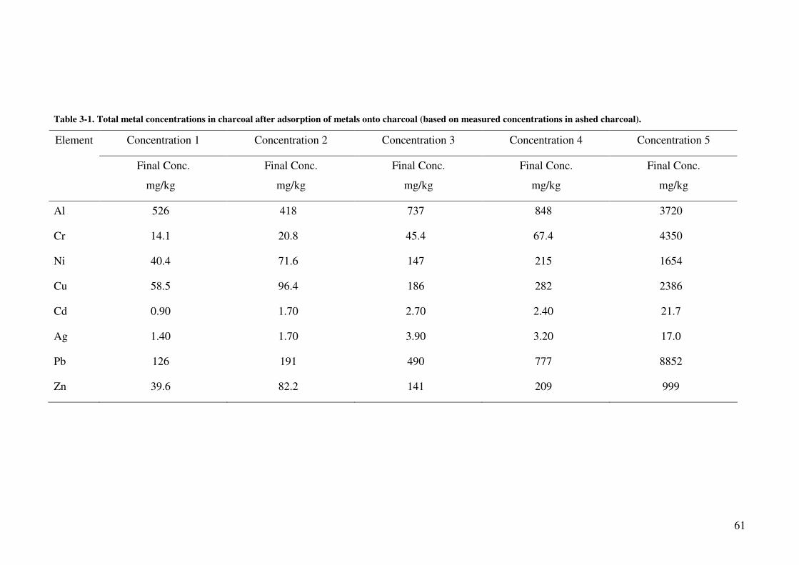
61

Table 3-1. Total metal concentrations in charcoal after adsorption of metals onto charcoal (based on measured concentrations in ashed charcoal).

Concentration 1 Concentration 2 Concentration 3 Concentration 4 Concentration 5 Element

Final Conc.

mg/kg

Final Conc.

mg/kg

Final Conc.

mg/kg

Final Conc.

mg/kg

Final Conc.

mg/kg

Al 526 418 737 848 3720

Cr 14.1 20.8 45.4 67.4 4350

Ni 40.4 71.6 147 215 1654

Cu 58.5 96.4 186 282 2386

Cd 0.90 1.70 2.70 2.40 21.7

Ag 1.40 1.70 3.90 3.20 17.0

Pb 126 191 490 777 8852

Zn 39.6 82.2 141 209 999

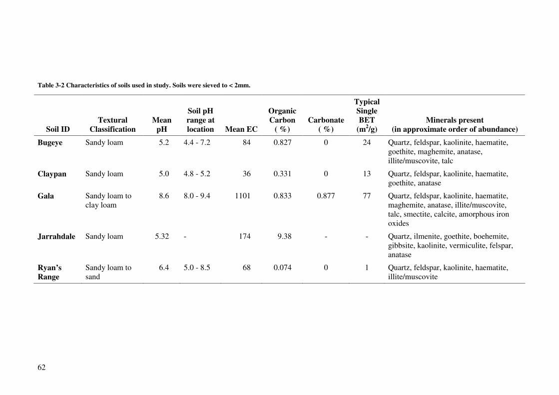
62

Table 3-2 Characteristics of soils used in study. Soils were sieved to < 2mm.

Soil ID

Textural

Classification

Mean

pH

Soil pH

range at

location Mean EC

Organic

Carbon

( %)

Carbonate

( %)

Typical

Single

BET

(m2/g)

Minerals present

(in approximate order of abundance)

Bugeye Sandy loam 5.2 4.4 - 7.2 84 0.827 0 24 Quartz, feldspar, kaolinite, haematite,

goethite, maghemite, anatase,

illite/muscovite, talc

Claypan Sandy loam 5.0 4.8 - 5.2 36 0.331 0 13 Quartz, feldspar, kaolinite, haematite,

goethite, anatase

Gala Sandy loam to

clay loam

8.6 8.0 - 9.4 1101 0.833 0.877 77 Quartz, feldspar, kaolinite, haematite,

maghemite, anatase, illite/muscovite,

talc, smectite, calcite, amorphous iron

oxides

Jarrahdale Sandy loam 5.32 - 174 9.38 - - Quartz, ilmenite, goethite, boehemite,

gibbsite, kaolinite, vermiculite, felspar,

anatase

Ryan’s

Range

Sandy loam to

sand

6.4 5.0 - 8.5 68 0.074 0 1 Quartz, feldspar, kaolinite, haematite,

illite/muscovite

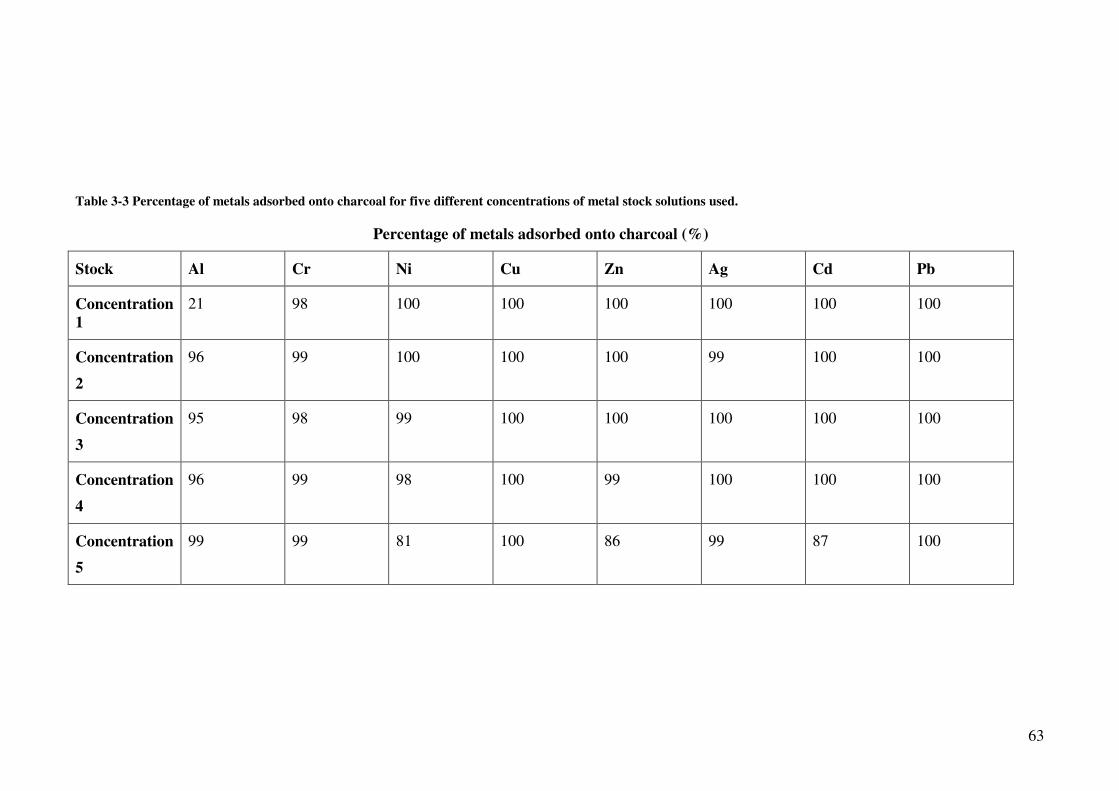
63

Table 3-3 Percentage of metals adsorbed onto charcoal for five different concentrations of metal stock solutions used.

Percentage of metals adsorbed onto charcoal (%)

Stock Al Cr Ni Cu Zn Ag Cd Pb

Concentration

1

21 98 100 100 100 100 100 100

Concentration

2

96 99 100 100 100 99 100 100

Concentration

3

95 98 99 100 100 100 100 100

Concentration

4

96 99 98 100 99 100 100 100

Concentration

5

99 99 81 100 86 99 87 100

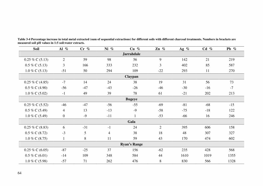
64

Table 3-4 Percentage increase in total metal extracted (sum of sequential extractions) for different soils with different charcoal treatments. Numbers in brackets are

measured soil pH values in 1:5 soil:water extracts.

Soil Al % Cr % Ni % Cu % Zn % Ag % Cd % Pb %

Jarrahdale

0.25 % C (5.13) 2 59 98 56 9 142 21 219

0.5 % C (5.13) 3 166 333 232 3 402 85 587

1.0 % C (5.13) -51 50 294 109 -22 293 11 270

Claypan

0.25 % C (4.85) -7 14 24 38 19 31 56 73

0.5 % C (4.90) -56 -47 -43 -26 -46 -30 -16 -7

1.0 % C (5.02) -1 49 39 78 61 -21 202 213

Bugeye

0.25 % C (5.52) -46 -47 -56 -55 -69 -81 -68 -15

0.5 % C (5.49) 4 13 -13 -9 -58 -75 -18 122

1.0 % C (5.49) 0 -9 -11 1 -53 -66 16 246

Gala

0.25 % C (8.83) 6 -31 -1 24 2 395 606 158

0.5 % C (8.72) -3 5 4 38 18 48 307 327

1.0 % C (8.75) 1 8 11 59 43 170 474 602

Ryan’s Range

0.25 % C (6.05) -87 -25 37 156 -62 235 428 568

0.5 % C (6.01) -14 109 348 584 44 1610 1019 1355

1.0 % C (5.98) -57 71 262 476 8 830 566 1328

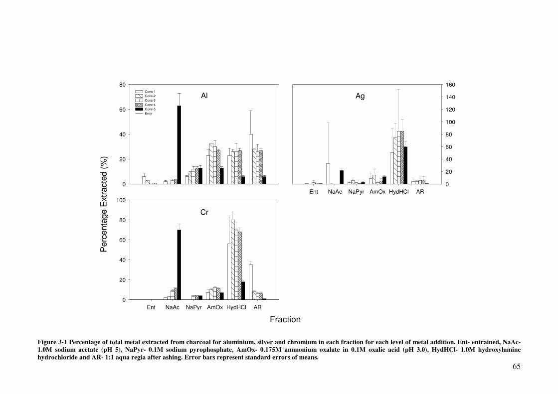
65

AlP

erc

enta

ge E

xtr

acte

d (

%)

0

20

40

60

80

Cr

Fraction

Ent NaAc NaPyr AmOx HydHCl AR

0

20

40

60

80

100

Ag


0

20

40

60

80

100

120

140

160Conc-1

Conc-2

Conc-3

Conc-4

Conc-5

Error

Figure 3-1 Percentage of total metal extracted from charcoal for aluminium, silver and chromium in each fraction for each level of metal addition. Ent- entrained, NaAc-

1.0M sodium acetate (pH 5), NaPyr- 0.1M sodium pyrophosphate, AmOx- 0.175M ammonium oxalate in 0.1M oxalic acid (pH 3.0), HydHCl- 1.0M hydroxylamine

hydrochloride and AR- 1:1 aqua regia after ashing. Error bars represent standard errors of means.

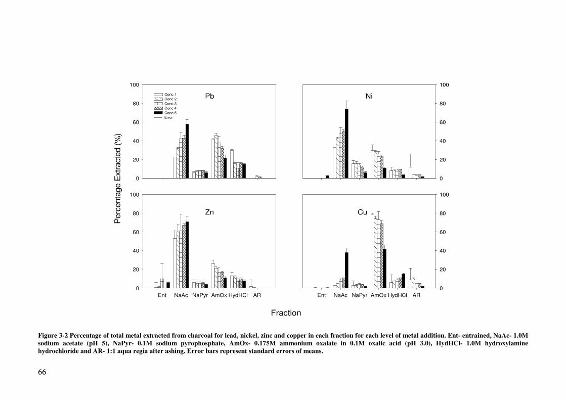
66

Zn


0

20

40

60

80

100

Ni

0

20

40

60

80

100

Pb

Perc

enta

ge E

xtr

acte

d (

%)

0

20

40

60

80

100

Conc 1

Conc 2

Conc 3

Conc 4

Conc 5

Error

Cu

Fraction


0

20

40

60

80

100

Figure 3-2 Percentage of total metal extracted from charcoal for lead, nickel, zinc and copper in each fraction for each level of metal addition. Ent- entrained, NaAc- 1.0M

sodium acetate (pH 5), NaPyr- 0.1M sodium pyrophosphate, AmOx- 0.175M ammonium oxalate in 0.1M oxalic acid (pH 3.0), HydHCl- 1.0M hydroxylamine

hydrochloride and AR- 1:1 aqua regia after ashing. Error bars represent standard errors of means.

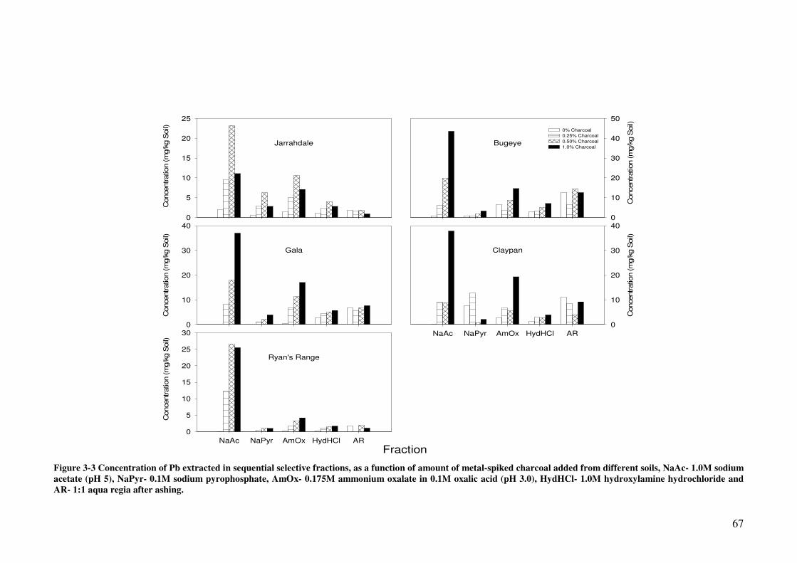
67

Bugeye

Concentration (m

g/k

g S

oil)

0

10

20

30

40

50

Jarrahdale

Concentration (m

g/k

g S

oil)

0

5

10

15

20

25

0% Charcoal

0.25% Charcoal

0.50% Charcoal

1.0% Charcoal

Gala

Concentration (m

g/k

g S

oil)

0

10

20

30

40

Claypan

NaAc NaPyr AmOx HydHCl AR

Concentration (m

g/k

g S

oil)

0

10

20

30

40

Ryan's Range

FractionNaAc NaPyr AmOx HydHCl AR

Concentration (m

g/k

g S

oil)

0

5

10

15

20

25

30

Figure 3-3 Concentration of Pb extracted in sequential selective fractions, as a function of amount of metal-spiked charcoal added from different soils, NaAc- 1.0M sodium

acetate (pH 5), NaPyr- 0.1M sodium pyrophosphate, AmOx- 0.175M ammonium oxalate in 0.1M oxalic acid (pH 3.0), HydHCl- 1.0M hydroxylamine hydrochloride and

AR- 1:1 aqua regia after ashing.

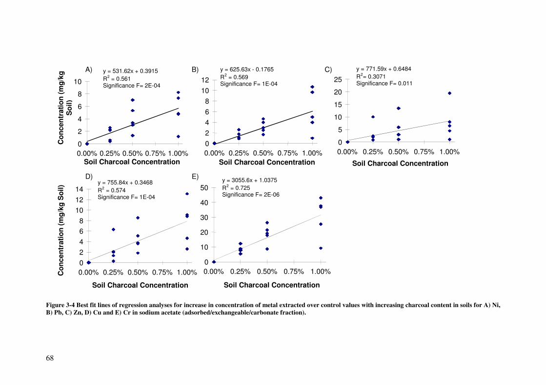
68

Figure 3-4 Best fit lines of regression analyses for increase in concentration of metal extracted over control values with increasing charcoal content in soils for A) Ni,

B) Pb, C) Zn, D) Cu and E) Cr in sodium acetate (adsorbed/exchangeable/carbonate fraction).

y = 531.62x + 0.3915 R 2 = 0.561 Significance F= 2E-04

0

2

4

6

8

10

0.00% 0.25% 0.50% 0.75% 1.00% Soil Charcoal Concentration

Co

ncen

trati

on

(m

g/k

g

So

il)

y = 771.59x + 0.6484 R 2 = 0.3071 Significance F= 0.011

0

5

10

15

20

25

0.00% 0.25% 0.50% 0.75% 1.00%

Soil Charcoal Concentration

y = 625.63x - 0.1765 R 2 = 0.569 Significance F= 1E-04

0

2

4

6

8

10

12

0.00% 0.25% 0.50% 0.75% 1.00%


y = 755.84x + 0.3468 R 2 = 0.574 Significance F= 1E-04

0

2

4

6

8

10

12

14

0.00% 0.25% 0.50% 0.75% 1.00%


Co

ncen

trati

on

(m

g/k

g S

oil

)

A) B) C)

D) E) y = 3055.6x + 1.0375 R 2 = 0.725 Significance F= 2E-06

0

10

20

30

40

50

0.00% 0.25% 0.50% 0.75% 1.00%


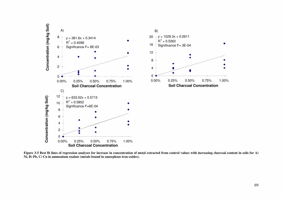
69

Figure 3-5 Best fit lines of regression analyses for increase in concentration of metal extracted from control values with increasing charcoal content in soils for A)

Ni, B) Pb, C) Cu in ammonium oxalate (metals bound in amorphous iron oxides).

y = 381.6x + 0.3414

R 2 = 0.4099

Significance F= 8E-03

0

2

4

6

8

0.00% 0.25% 0.50% 0.75% 1.00%


Co

ncen

trati

on

(m

g/k

g S

oil

)

y = 633.02x + 0.5715

R 2 = 0.5852

Significance F=6E-04

0

2

4

6

8

10

12

0.00% 0.25% 0.50% 0.75% 1.00%


Co

ncen

trati

on

(m

g/k

g S

oil

)

y = 1029.3x + 0.0911

R 2

= 0.5262

Significance F= 3E-04

0

4

8

12

16

20

0.00% 0.25% 0.50% 0.75% 1.00%


A)

C)

B)

71

CHAPTER FOUR

Field study on biogeochemistry and the formation of soil geochemical

anomalies I.: Berkley Prospect, Coolgardie, Western Australia

4. Introduction

Locating ore deposits hidden beneath a transported overburden is an ongoing challenge

for the mining industry. In mineralised areas, localised concentrations of ore-related

elements, relative to background concentrations in barren areas, occur in soils through

the weathering of parent material. However, in situations where an exotic overburden

has been deposited over the original or eroded land surface, anomalies of ore and/or

pathfinder elements may or may not be present in the surface soils. The development of

surface soil anomalies would subsequently depend on the establishment of a net vertical

ionic transport flux through the transported overburden. Several physico-chemical

processes have been put forth to account for the migration of elements into the

overburden (Govett 1976; Hamilton 1998; Kelley et al. 2006). Although a significant

body of research exists on the effects of biota on metal migration from depth to surface,

considerably less is known regarding transfer of metals from vegetation into the soil and

development of, or contribution to, soil anomalies (Dunn 1981; Dunn 1986; Cohen et

al. 1999; Kelley et al. 2006).

There is ample evidence that vegetation can affect trace element mobility in the regolith

by physically and chemically altering its immediate environment (Dakora et al. 2002;

Stretch et al. 2002). Plants are also able to root down to great depths in search of

nutrients and water (Canadell et al. 1996) and could penetrate tens of metres of

transported cover (Rose et al. 1979). Given a sufficiently long time span (>106 yrs), the

uptake of ions by vegetation at depth in the regolith and the subsequent return of plant

matter to the soil would eventually lead to the concentration of trace elements in the

surface soil. However, it is difficult to directly measure this “deep uptake” flux by

vegetation and indirect evidence through careful selection of study sites, in which this

deep uptake flux would be expected to dominate, was sought.

In order to test the hypothesis that biological uptake leads to the accumulation of trace

elements in the surface soil, we attempted to locate field sites in which the vertical

transport of elements in the regolith by physical processes would be minimal (see also

similar study by Lintern (2007)). Hence, an ideal field site in which biological transport

72

would dominate would display the following characteristics: 1) Located in a flat and

stable landscape in order to minimise physical loss (e.g. erosion) from the system; 2)

Located in an arid or semi-arid environment to minimise the likelihood of element

transport through the regolith by hydrodynamic dispersion and to minimise drainage

loss, with 3) an appropriately low water table depth, (>15 m) (See Chapter 2 for

justification and Keeling (2004); and 4) Has a transported overburden present to

minimise the likelihood of a residual signature from the mineralisation.

This chapter presents the first of two field studies carried out in semi-arid Western

Australia. In the chapter, the results of soil and vegetation analyses in transects across

mineralised prospects from the first field study site near Coolgardie, Western Australia

are discussed. The aims of the field study at Berkley were: i) To determine if deep biotic

uplift of Au has led to the accumulation of trace elements in the surface soils developed

from the transported overburden; ii) To determine if the vegetation and soils show

geochemical responses to the changing lithology underneath the transported overburden

and; iii) To generate input data for numerical modelling.

4.1. Materials and Methods

4.1.1. Field Sampling

4.1.1.1. Site description

The Forrest Gold and Miriam North prospects, collectively known as the Berkley

Prospect, are located near Coolgardie, approximately 550 km east of Perth in Western

Australia. The region receives about 270 mm mean annual rainfall (Bureau of

Meteorology Australia 2007). Vegetation in the prospects consists of mixed stands of

eucalypts (Eucalyptus sheathiana, Eucalyptus salmonphloia, Eucalyptus cylindricarpa,

Eucalyptus lesouefii) (See Plate 4-1). Sampling at the Forrest Gold and Miriam North

prospects was carried along two parallel transects, 6563 125N and 6563 350N (GPS

database: UTM ’84). Transect 6563 125N passes over four distinct lithological units. In

the west, the transect passes over poorly exposed cumulate facies ultramafics. A steeply

dipping bedrock contact between these ultramafics and metabasalt exists at

approximately 318 970E and both sampling transects run perpendicularly to this

contact. Historical drilling has shown that there are scattered nickel sulphide intercepts

close to this contact (the Mirriam Nickel Prospect) that are discontinuous (L. Bettany

(pers comm.). A second bedrock contact with ultramafic pyroxenite on a poorly exposed

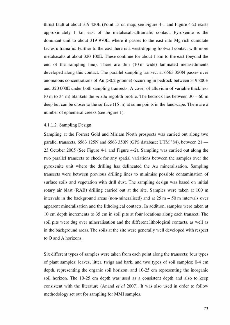
73

thrust fault at about 319 420E (Point 13 on map; see Figure 4-1 and Figure 4-2) exists

approximately 1 km east of the metabasalt-ultramafic contact. Pyroxenite is the

dominant unit to about 319 970E, where it passes to the east into Mg-rich cumulate

facies ultramafic. Further to the east there is a west-dipping footwall contact with more

metabasalts at about 320 100E. These continue for about 1 km to the east (beyond the

end of the sampling line). There are thin (10 m wide) laminated metasediments

developed along this contact. The parallel sampling transect at 6563 350N passes over

anomalous concentrations of Au (>0.2 g/tonne) occurring in bedrock between 319 800E

and 320 000E under both sampling transects. A cover of alluvium of variable thickness

(0 m to 34 m) blankets the in situ regolith profile. The bedrock lies between 30 – 60 m

deep but can be closer to the surface (15 m) at some points in the landscape. There are a

number of ephemeral creeks (see Figure 1).

4.1.1.2. Sampling Design

Sampling at the Forrest Gold and Miriam North prospects was carried out along two

parallel transects, 6563 125N and 6563 350N (GPS database: UTM ’84), between 21 —

23 October 2005 (See Figure 4-1 and Figure 4-2). Sampling was carried out along the

two parallel transects to check for any spatial variations between the samples over the

pyroxenite unit where the drilling has delineated the Au mineralisation. Sampling

transects were between previous drilling lines to minimise possible contamination of

surface soils and vegetation with drill dust. The sampling design was based on initial

rotary air blast (RAB) drilling carried out at the site. Samples were taken at 100 m

intervals in the background areas (non-mineralised) and at 25 m – 50 m intervals over

apparent mineralisation and the lithological contacts. In addition, samples were taken at

10 cm depth increments to 35 cm in soil pits at four locations along each transect. The

soil pits were dug over mineralisation and the different lithological contacts, as well as

in the background areas. The soils at the site were generally well developed with respect

to O and A horizons.

Six different types of samples were taken from each point along the transects; four types

of plant samples: leaves, litter, twigs and bark, and two types of soil samples; 0-4 cm

depth, representing the organic soil horizon, and 10-25 cm representing the inorganic

soil horizon. The 10-25 cm depth was used as a consistent depth and also to keep

consistent with the literature (Anand et al 2007). It was also used in order to follow

methodology set out for sampling for MMI samples.

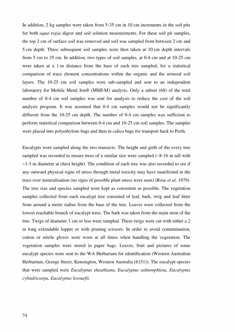
74

In addition, 2 kg samples were taken from 5-35 cm in 10 cm increments in the soil pits

for both aqua regia digest and soil solution measurements. For these soil pit samples,

the top 2 cm of surface soil was removed and soil was sampled from between 2 cm and

5 cm depth. Three subsequent soil samples were then taken at 10 cm depth intervals

from 5 cm to 35 cm. In addition, two types of soil samples, at 0-4 cm and at 10-25 cm

were taken at a 1 m distance from the base of each tree sampled, for a statistical

comparison of trace element concentrations within the organic and the mineral soil

layers. The 10-25 cm soil samples were sub-sampled and sent to an independent

laboratory for Mobile Metal Ion® (MMI-M) analysis. Only a subset (68) of the total

number of 0-4 cm soil samples was sent for analysis to reduce the cost of the soil

analysis program. It was assumed that 0-4 cm samples would not be significantly

different from the 10-25 cm depth. The number of 0-4 cm samples was sufficient to

perform statistical comparison between 0-4 cm and 10-25 cm soil samples. The samples

were placed into polyethylene bags and then in calico bags for transport back to Perth.

Eucalypts were sampled along the two transects. The height and girth of the every tree

sampled was recorded to ensure trees of a similar size were sampled (~8-16 m tall with

~1-3 m diameter at chest height). The condition of each tree was also recorded to see if

any outward physical signs of stress through metal toxicity may have manifested in the

trees over mineralisation (no signs of possible plant stress were seen) (Rose et al. 1979).

The tree size and species sampled were kept as consistent as possible. The vegetation

samples collected from each eucalypt tree consisted of leaf, bark, twig and leaf litter

from around a metre radius from the base of the tree. Leaves were collected from the

lowest reachable branch of eucalypt trees. The bark was taken from the main stem of the

tree. Twigs of diameter 1 cm or less were sampled. These twigs were cut with either a 2

m long extendable lopper or with pruning scissors. In order to avoid contamination,

cotton or nitrile gloves were worn at all times when handling the vegetation. The

vegetation samples were stored in paper bags. Leaves, fruit and pictures of some

eucalypt species were sent to the WA Herbarium for identification (Western Australian

Herbarium, George Street, Kensington, Western Australia (6151)). The eucalypt species

that were sampled were Eucalyptus sheathiana, Eucalyptus salmonphloia, Eucalyptus

cylindricarpa, Eucalyptus lesouefii.

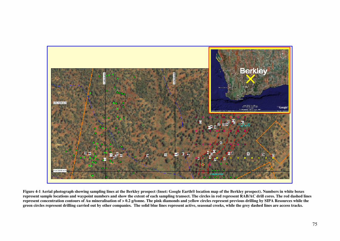
75

Figure 4-1 Aerial photograph showing sampling lines at the Berkley prospect (Inset: Google Earth® location map of the Berkley prospect). Numbers in white boxes

represent sample locations and waypoint numbers and show the extent of each sampling transect. The circles in red represent RAB/AC drill cores. The red dashed lines

represent concentration contours of Au mineralisation of > 0.2 g/tonne. The pink diamonds and yellow circles represent previous drilling by SIPA Resources while the

green circles represent drilling carried out by other companies. The solid blue lines represent active, seasonal creeks, while the grey dashed lines are access tracks.

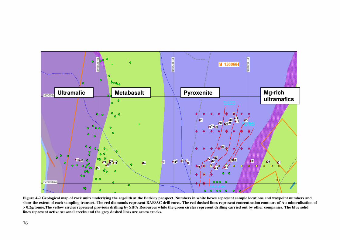
76

Figure 4-2 Geological map of rock units underlying the regolith at the Berkley prospect. Numbers in white boxes represent sample locations and waypoint numbers and

show the extent of each sampling transect. The red diamonds represent RAB/AC drill cores. The red dashed lines represent concentration contours of Au mineralisation of

> 0.2g/tonne.The yellow circles represent previous drilling by SIPA Resources while the green circles represent drilling carried out by other companies. The blue solid

lines represent active seasonal creeks and the grey dashed lines are access tracks.

Metabasalt Ultramafic Pyroxenite Mg-rich ultramafics

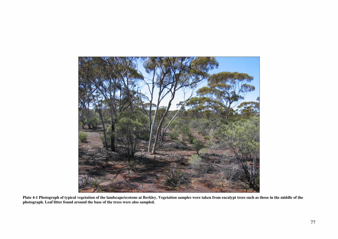
77

Plate 4-1 Photograph of typical vegetation of the landscape/ecotone at Berkley. Vegetation samples were taken from eucalypt trees such as those in the middle of the

photograph. Leaf litter found around the base of the trees were also sampled.

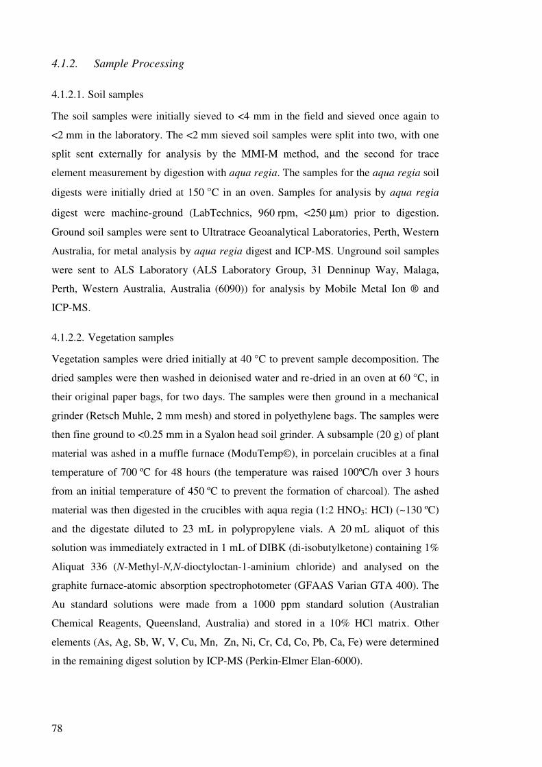
78

4.1.2. Sample Processing

4.1.2.1. Soil samples

The soil samples were initially sieved to <4 mm in the field and sieved once again to

<2 mm in the laboratory. The <2 mm sieved soil samples were split into two, with one

split sent externally for analysis by the MMI-M method, and the second for trace

element measurement by digestion with aqua regia. The samples for the aqua regia soil

digests were initially dried at 150 °C in an oven. Samples for analysis by aqua regia

digest were machine-ground (LabTechnics, 960 rpm, <250 µm) prior to digestion.

Ground soil samples were sent to Ultratrace Geoanalytical Laboratories, Perth, Western

Australia, for metal analysis by aqua regia digest and ICP-MS. Unground soil samples

were sent to ALS Laboratory (ALS Laboratory Group, 31 Denninup Way, Malaga,

Perth, Western Australia, Australia (6090)) for analysis by Mobile Metal Ion ® and

ICP-MS.

4.1.2.2. Vegetation samples

Vegetation samples were dried initially at 40 °C to prevent sample decomposition. The

dried samples were then washed in deionised water and re-dried in an oven at 60 °C, in

their original paper bags, for two days. The samples were then ground in a mechanical

grinder (Retsch Muhle, 2 mm mesh) and stored in polyethylene bags. The samples were

then fine ground to <0.25 mm in a Syalon head soil grinder. A subsample (20 g) of plant

material was ashed in a muffle furnace (ModuTemp©), in porcelain crucibles at a final

temperature of 700 ºC for 48 hours (the temperature was raised 100ºC/h over 3 hours

from an initial temperature of 450 ºC to prevent the formation of charcoal). The ashed

material was then digested in the crucibles with aqua regia (1:2 HNO3: HCl) (~130 ºC)

and the digestate diluted to 23 mL in polypropylene vials. A 20 mL aliquot of this

solution was immediately extracted in 1 mL of DIBK (di-isobutylketone) containing 1%

Aliquat 336 (N-Methyl-N,N-dioctyloctan-1-aminium chloride) and analysed on the

graphite furnace-atomic absorption spectrophotometer (GFAAS Varian GTA 400). The

Au standard solutions were made from a 1000 ppm standard solution (Australian

Chemical Reagents, Queensland, Australia) and stored in a 10% HCl matrix. Other

elements (As, Ag, Sb, W, V, Cu, Mn, Zn, Ni, Cr, Cd, Co, Pb, Ca, Fe) were determined

in the remaining digest solution by ICP-MS (Perkin-Elmer Elan-6000).

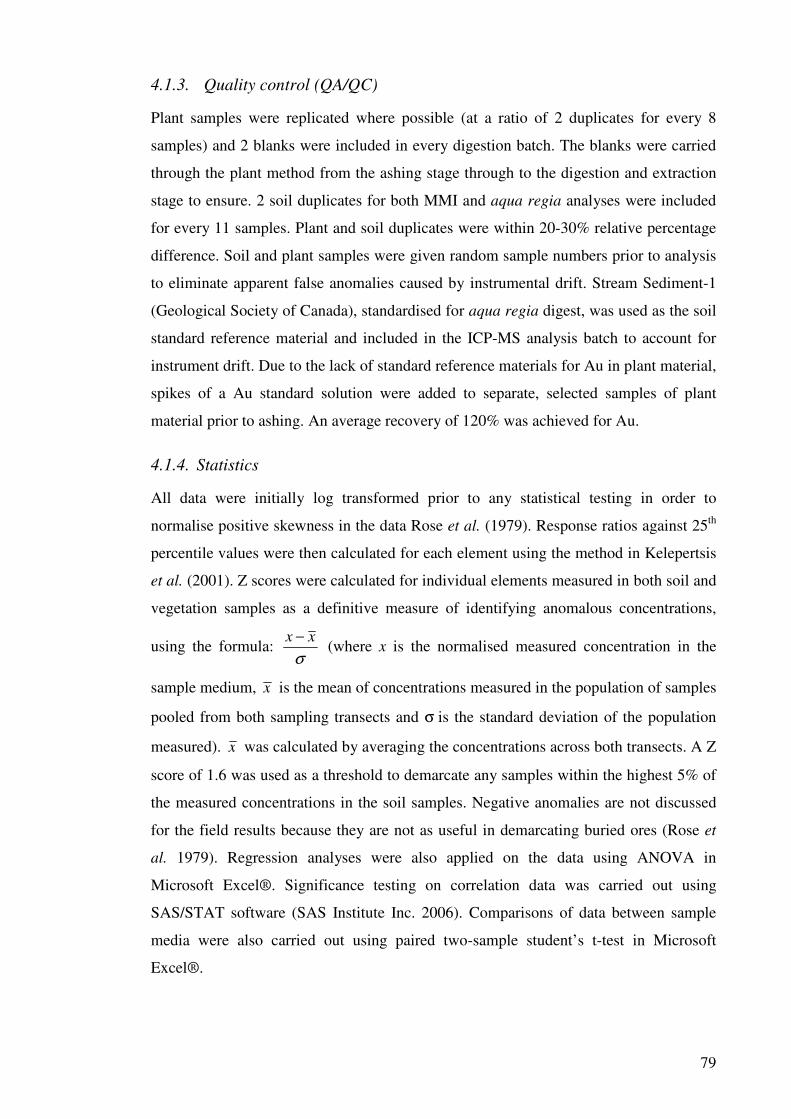
79

4.1.3. Quality control (QA/QC)

Plant samples were replicated where possible (at a ratio of 2 duplicates for every 8

samples) and 2 blanks were included in every digestion batch. The blanks were carried

through the plant method from the ashing stage through to the digestion and extraction

stage to ensure. 2 soil duplicates for both MMI and aqua regia analyses were included

for every 11 samples. Plant and soil duplicates were within 20-30% relative percentage

difference. Soil and plant samples were given random sample numbers prior to analysis

to eliminate apparent false anomalies caused by instrumental drift. Stream Sediment-1

(Geological Society of Canada), standardised for aqua regia digest, was used as the soil

standard reference material and included in the ICP-MS analysis batch to account for

instrument drift. Due to the lack of standard reference materials for Au in plant material,

spikes of a Au standard solution were added to separate, selected samples of plant

material prior to ashing. An average recovery of 120% was achieved for Au.

4.1.4. Statistics

All data were initially log transformed prior to any statistical testing in order to

normalise positive skewness in the data Rose et al. (1979). Response ratios against 25th

percentile values were then calculated for each element using the method in Kelepertsis

et al. (2001). Z scores were calculated for individual elements measured in both soil and

vegetation samples as a definitive measure of identifying anomalous concentrations,

using the formula: σ

xx −

(where x is the normalised measured concentration in the

sample medium, x is the mean of concentrations measured in the population of samples

pooled from both sampling transects and σ is the standard deviation of the population

measured). x was calculated by averaging the concentrations across both transects. A Z

score of 1.6 was used as a threshold to demarcate any samples within the highest 5% of

the measured concentrations in the soil samples. Negative anomalies are not discussed

for the field results because they are not as useful in demarcating buried ores (Rose et

al. 1979). Regression analyses were also applied on the data using ANOVA in

Microsoft Excel®. Significance testing on correlation data was carried out using

SAS/STAT software (SAS Institute Inc. 2006). Comparisons of data between sample

media were also carried out using paired two-sample student’s t-test in Microsoft

Excel®.

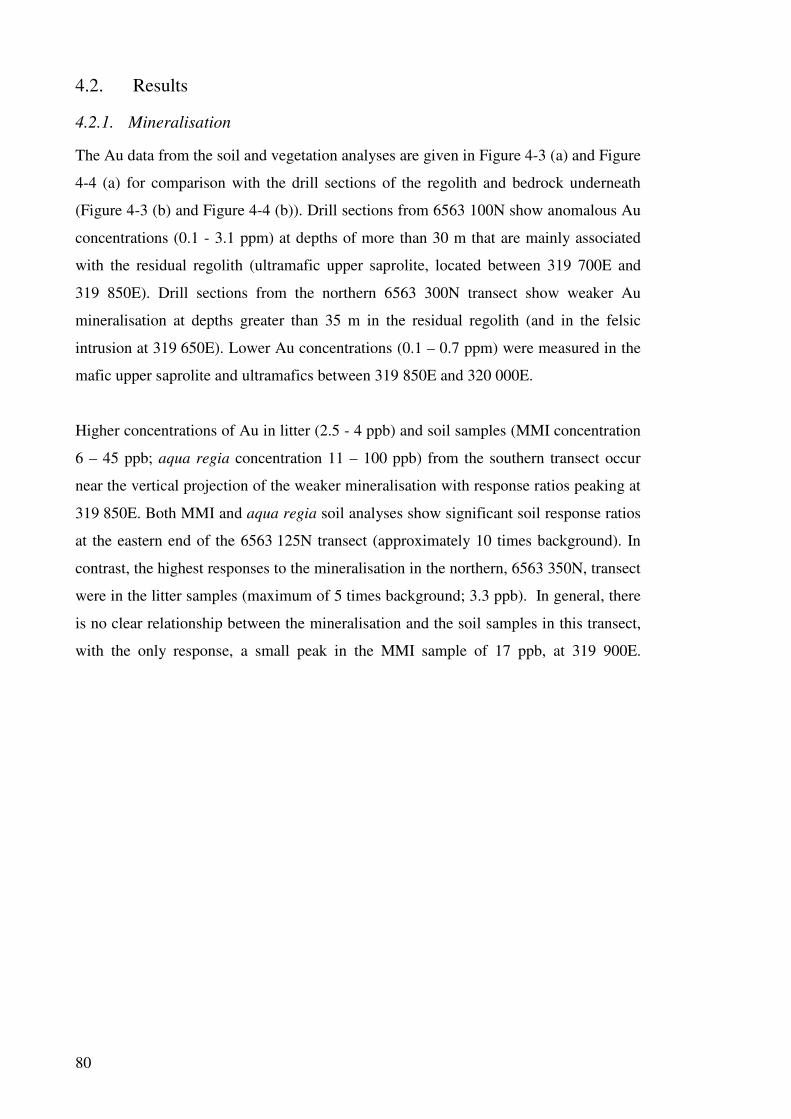
80

4.2. Results

4.2.1. Mineralisation

The Au data from the soil and vegetation analyses are given in Figure 4-3 (a) and Figure

4-4 (a) for comparison with the drill sections of the regolith and bedrock underneath

(Figure 4-3 (b) and Figure 4-4 (b)). Drill sections from 6563 100N show anomalous Au

concentrations (0.1 - 3.1 ppm) at depths of more than 30 m that are mainly associated

with the residual regolith (ultramafic upper saprolite, located between 319 700E and

319 850E). Drill sections from the northern 6563 300N transect show weaker Au

mineralisation at depths greater than 35 m in the residual regolith (and in the felsic

intrusion at 319 650E). Lower Au concentrations (0.1 – 0.7 ppm) were measured in the

mafic upper saprolite and ultramafics between 319 850E and 320 000E.

Higher concentrations of Au in litter (2.5 - 4 ppb) and soil samples (MMI concentration

6 – 45 ppb; aqua regia concentration 11 – 100 ppb) from the southern transect occur

near the vertical projection of the weaker mineralisation with response ratios peaking at

319 850E. Both MMI and aqua regia soil analyses show significant soil response ratios

at the eastern end of the 6563 125N transect (approximately 10 times background). In

contrast, the highest responses to the mineralisation in the northern, 6563 350N, transect

were in the litter samples (maximum of 5 times background; 3.3 ppb). In general, there

is no clear relationship between the mineralisation and the soil samples in this transect,

with the only response, a small peak in the MMI sample of 17 ppb, at 319 900E.

81

(a)

0

2

4

6

8

10

12

14

16

18

319550 319600 319650 319700 319750 319800 319850 319900 319950 320000 320050

Easting

Re

sp

on

se

ra

tio

Soil, MMI

Litter

Leaf

Soil, Aqua Regia

(b)

-70

-60

-50

-40

-30

-20

-10

0

319550 319600 319650 319700 319750 319800 319850 319900 319950 320000

Easting

De

pth

m

1.0ppm 1.1ppm

2.4ppm

3.1ppm0.2ppm0.2ppm0.2ppm

0.2ppm0.1ppm

Mafics

Ultramafic upper saprolite

Mafic upper saprolite

Transported Overburden

Felsics

KEY

Ultramafics

xppm Au concentration

Figure 4-3 (a) Au response in different media between 319 600E and 320 000E on the southern

transect, 6563 125N. (b) Drill sections from drill line 6563 100N. Red numbers in boxes represent

the average concentration of Au measured in 5 m depths (Note: Only anomalous Au concentrations

are shown in the figure). The position of each box represents the approximate depth at which the

Au was measured in the drill core. Actual mean concentrations of Au measured in transported

overburden are attached in the appendix section.

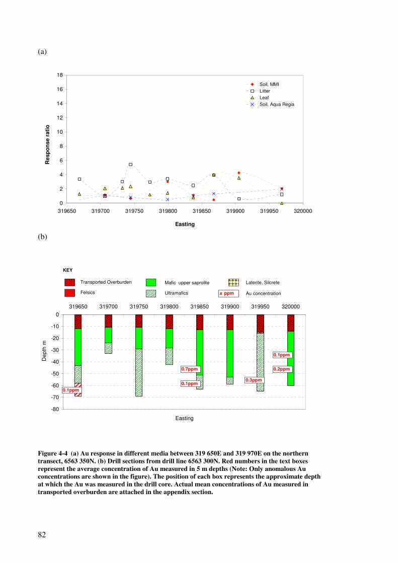
82

(a)

0

2

4

6

8

10

12

14

16

18

319650 319700 319750 319800 319850 319900 319950 320000

Easting

Re

sp

on

se

ra

tio

Soil, MMI

Litter

Leaf

Soil, Aqua Regia

(b)

-80

-70

-60

-50

-40

-30

-20

-10

0

319650 319700 319750 319800 319850 319900 319950 320000

Easting

De

pth

m

0.1ppm

0.1ppm

0.7ppm

0.3ppm

Transported Overburden

UltramaficsFelsics

Mafic upper saprolite

KEY

Laterite, Silcrete

x ppm Au concentration

0.2ppm

0.1ppm

Figure 4-4 (a) Au response in different media between 319 650E and 319 970E on the northern

transect, 6563 350N. (b) Drill sections from drill line 6563 300N. Red numbers in the text boxes

represent the average concentration of Au measured in 5 m depths (Note: Only anomalous Au

concentrations are shown in the figure). The position of each box represents the approximate depth

at which the Au was measured in the drill core. Actual mean concentrations of Au measured in

transported overburden are attached in the appendix section.

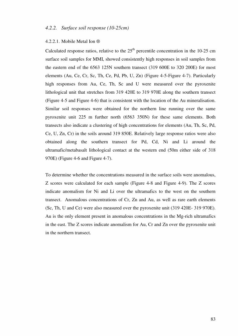
83

4.2.2. Surface soil response (10-25cm)

4.2.2.1. Mobile Metal Ion ®

Calculated response ratios, relative to the 25th

percentile concentration in the 10-25 cm

surface soil samples for MMI, showed consistently high responses in soil samples from

the eastern end of the 6563 125N southern transect (319 600E to 320 200E) for most

elements (Au, Ce, Cr, Sc, Th, Ce, Pd, Pb, U, Zn) (Figure 4-5-Figure 4-7). Particularly

high responses from Au, Ce, Th, Sc and U were measured over the pyroxenite

lithological unit that stretches from 319 420E to 319 970E along the southern transect

(Figure 4-5 and Figure 4-6) that is consistent with the location of the Au mineralisation.

Similar soil responses were obtained for the northern line running over the same

pyroxenite unit 225 m further north (6563 350N) for these same elements. Both

transects also indicate a clustering of high concentrations for elements (Au, Th, Sc, Pd,

Ce, U, Zn, Cr) in the soils around 319 850E. Relatively large response ratios were also

obtained along the southern transect for Pd, Cd, Ni and Li around the

ultramafic/metabasalt lithological contact at the western end (50m either side of 318

970E) (Figure 4-6 and Figure 4-7).

To determine whether the concentrations measured in the surface soils were anomalous,

Z scores were calculated for each sample (Figure 4-8 and Figure 4-9). The Z scores

indicate anomalism for Ni and Li over the ultramafics to the west on the southern

transect. Anomalous concentrations of Cr, Zn and Au, as well as rare earth elements

(Sc, Th, U and Ce) were also measured over the pyroxenite unit (319 420E- 319 970E).

Au is the only element present in anomalous concentrations in the Mg-rich ultramafics

in the east. The Z scores indicate anomalism for Au, Cr and Zn over the pyroxenite unit

in the northern transect.

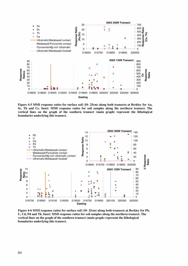
84

6563 125N Transect

0

1020

30

4050

60

7080

90

318600 318800 319000 319200 319400 319600 319800 320000 320200 320400 320600

Easting

Re

sp

on

se

Rati

os

0

100200

300

400500

600

700800

900

Ce

Re

sp

on

se

Rati

o

Au

Sc

Th

Ce

Ultramafic/Metabasalt contact

Metabasalt/Pyroxenite contact

Pyroxenite/Mg-rich Ultramafic

Ultramafic/Metabasalt footwall

6563 350N Transect

0

5

10

15

20

25

319650 319750 319850 319950 320050

Re

sp

on

se

Ra

tio

(Au

,Sc

)

0

100

200

300

400

500

600

700

Re

sp

on

se

Ra

tio

(Ce

, T

h)

Figure 4-5 MMI response ratios for surface soil (10- 25cm) along both transects at Berkley for Au,

Sc, Th and Ce. Inset: MMI response ratios for soil samples along the northern transect. The

vertical lines on the graph of the southern transect (main graph) represent the lithological

boundaries underlying this transect.

6563 125N Transect

0

2

4

6

8

10

12

14

318700 318900 319100 319300 319500 319700 319900 320100 320300 320500Easting

Re

sp

on

se

Ra

tio

0

10

2030

40

50

6070

8090 U

Res

po

ns

e

Rati

o

PbUCdPdThUltramafic/Metabasalt contactMetabasalt/Pyroxenite contactPyroxenite/Mg-rich Ultramafic contactUltramafic/Metabasalt footwall

6563 350N Transect

0

2

4

6

8

10

12

14

319600 319700 319800 319900 320000

Re

sp

on

se R

ati

o

0

20

40

60

80

100

120

140

Figure 4-6 MMI response ratios for surface soil (10- 25cm) along both transects at Berkley for Pb,

U, Cd, Pd and Th. Inset: MMI response ratios for soil samples along the northern transect. The

vertical lines on the graph of the southern transect (main graph) represent the lithological

boundaries underlying this transect.

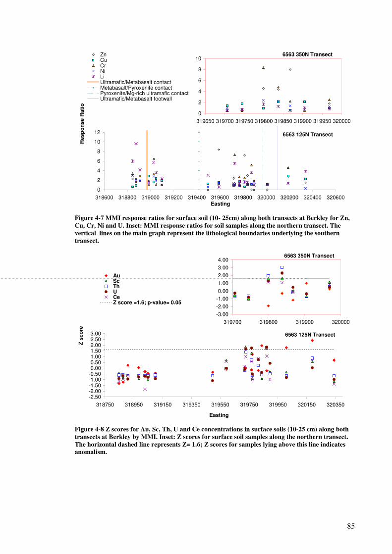
85

6563 125N Transect

0

2

4

6

8

10

12

318600 318800 319000 319200 319400 319600 319800 320000 320200 320400 320600Easting

Res

po

ns

e R

ati

o

ZnCuCrNiLiUltramafic/Metabasalt contactMetabasalt/Pyroxenite contactPyroxenite/Mg-rich ultramafic contactUltramafic/Metabasalt footwall

6563 350N Transect

0

2

4

6

8

10

319650 319700 319750 319800 319850 319900 319950 320000

Figure 4-7 MMI response ratios for surface soil (10- 25cm) along both transects at Berkley for Zn,

Cu, Cr, Ni and U. Inset: MMI response ratios for soil samples along the northern transect. The

vertical lines on the main graph represent the lithological boundaries underlying the southern

transect.

6563 125N Transect

-2.50-2.00-1.50-1.00-0.500.000.501.001.502.002.503.00

318750 318950 319150 319350 319550 319750 319950 320150 320350

Easting

Z s

co

re

AuScThUCeZ score =1.6; p-value= 0.05

6563 350N Transect

-3.00

-2.00

-1.00

0.00

1.00

2.00

3.00

4.00

319700 319800 319900 320000

Figure 4-8 Z scores for Au, Sc, Th, U and Ce concentrations in surface soils (10-25 cm) along both

transects at Berkley by MMI. Inset: Z scores for surface soil samples along the northern transect.

The horizontal dashed line represents Z= 1.6; Z scores for samples lying above this line indicates

anomalism.

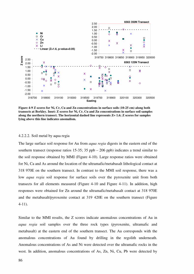
86

6563 125N Transect

-2.00

-1.50

-1.00

-0.50

0.00

0.50

1.00

1.50

2.00

2.50

318700 318900 319100 319300 319500 319700 319900 320100 320300 320500Easting

Z s

co

re

NiCrCuZnLiLinear (Z=1.6, p-value=0.05)

6563 350N Transect

-2.00

-1.50

-1.00

-0.50

0.00

0.50

1.00

1.50

2.00

2.50

319750 319800 319850 319900 319950 320000

Figure 4-9 Z scores for Ni, Cr, Cu and Zn concentrations in surface soils (10-25 cm) along both

transects at Berkley. Inset: Z scores for Ni, Cr, Cu and Zn concentrations in surface soil samples

along the northern transect. The horizontal dashed line represents Z= 1.6; Z scores for samples

lying above this line indicates anomalism.

4.2.2.2. Soil metal by aqua regia

The large surface soil response for Au from aqua regia digests in the eastern end of the

southern transect (response ratios 15-35; 35 ppb – 206 ppb) indicates a trend similar to

the soil response obtained by MMI (Figure 4-10). Large response ratios were obtained

for Ni, Ca and As around the location of the ultramafic/metabasalt lithological contact at

318 970E on the southern transect. In contrast to the MMI soil response, there was a

low aqua regia soil response for surface soils over the pyroxenite unit from both

transects for all elements measured (Figure 4-10 and Figure 4-11). In addition, high

responses were obtained for Zn around the ultramafic/metabasalt contact at 318 970E

and the metabasalt/pyroxenite contact at 319 420E on the southern transect (Figure

4-11).

Similar to the MMI results, the Z scores indicate anomalous concentrations of Au in

aqua regia soil samples over the three rock types (pyroxenite, ultramafic and

metabasalt) at the eastern end of the southern transect. The Au corresponds with the

anomalous concentrations of Au found by drilling in the regolith underneath.

Anomalous concentrations of As and Ni were detected over the ultramafic rocks in the

west. In addition, anomalous concentrations of As, Zn, Ni, Cu, Pb were detected by

87

aqua regia digests of surface soils along the ultramafic/metabasalt contact (at 318

970E) but not in the rest of the metabasalt unit to the east of the contact (Figure 4-12).

No anomalism was measured in the surface soils for these elements by aqua regia in the

northern transect.

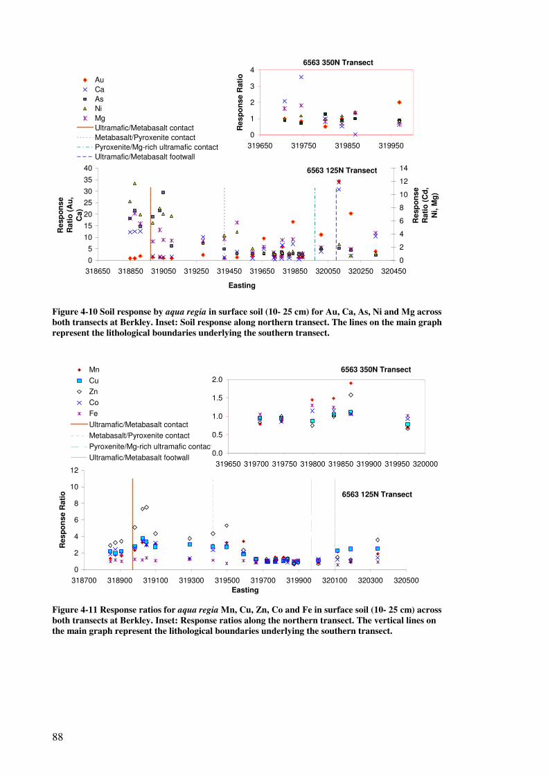
88

6563 125N Transect

0

5

10

15

20

25

30

35

40

318650 318850 319050 319250 319450 319650 319850 320050 320250 320450

Easting

Re

sp

on

se

Ra

tio

(A

u,

Ca

)

0

2

4

6

8

10

12

14

Re

sp

on

se

Ra

tio

(C

d,

Ni,

Mg

)

Au

Ca

As

Ni

Mg



Pyroxenite/Mg-rich ultramafic contact


6563 350N Transect

0

1

2

3

4

319650 319750 319850 319950

Re

sp

on

se

Rati

o

Figure 4-10 Soil response by aqua regia in surface soil (10- 25 cm) for Au, Ca, As, Ni and Mg across

both transects at Berkley. Inset: Soil response along northern transect. The lines on the main graph

represent the lithological boundaries underlying the southern transect.

6563 125N Transect

0

2

4

6

8

10

12

318700 318900 319100 319300 319500 319700 319900 320100 320300 320500

Easting

Re

sp

on

se

Ra

tio

Mn

Cu

Zn

Co

Fe





6563 350N Transect

0.0

0.5

1.0

1.5

2.0

319650 319700 319750 319800 319850 319900 319950 320000

Figure 4-11 Response ratios for aqua regia Mn, Cu, Zn, Co and Fe in surface soil (10- 25 cm) across

both transects at Berkley. Inset: Response ratios along the northern transect. The vertical lines on

the main graph represent the lithological boundaries underlying the southern transect.

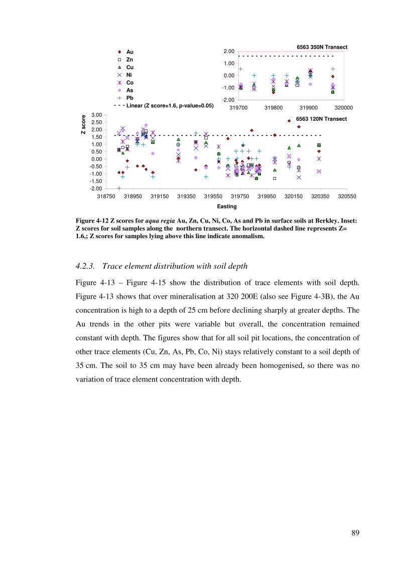
89

6563 120N Transect

-2.00

-1.50

-1.00

-0.50

0.00

0.50

1.00

1.50

2.00

2.50

3.00

318750 318950 319150 319350 319550 319750 319950 320150 320350 320550

Easting

Z s

co

re

Au

Zn

Cu

Ni

Co

As

Pb

Linear (Z score=1.6, p-value=0.05)

6563 350N Transect

-2.00

-1.00

0.00

1.00

2.00

319700 319800 319900 320000

Figure 4-12 Z scores for aqua regia Au, Zn, Cu, Ni, Co, As and Pb in surface soils at Berkley. Inset:

Z scores for soil samples along the northern transect. The horizontal dashed line represents Z=

1.6,; Z scores for samples lying above this line indicate anomalism.

4.2.3. Trace element distribution with soil depth

Figure 4-13 – Figure 4-15 show the distribution of trace elements with soil depth.

Figure 4-13 shows that over mineralisation at 320 200E (also see Figure 4-3B), the Au

concentration is high to a depth of 25 cm before declining sharply at greater depths. The

Au trends in the other pits were variable but overall, the concentration remained

constant with depth. The figures show that for all soil pit locations, the concentration of

other trace elements (Cu, Zn, As, Pb, Co, Ni) stays relatively constant to a soil depth of

35 cm. The soil to 35 cm may have been already been homogenised, so there was no

variation of trace element concentration with depth.

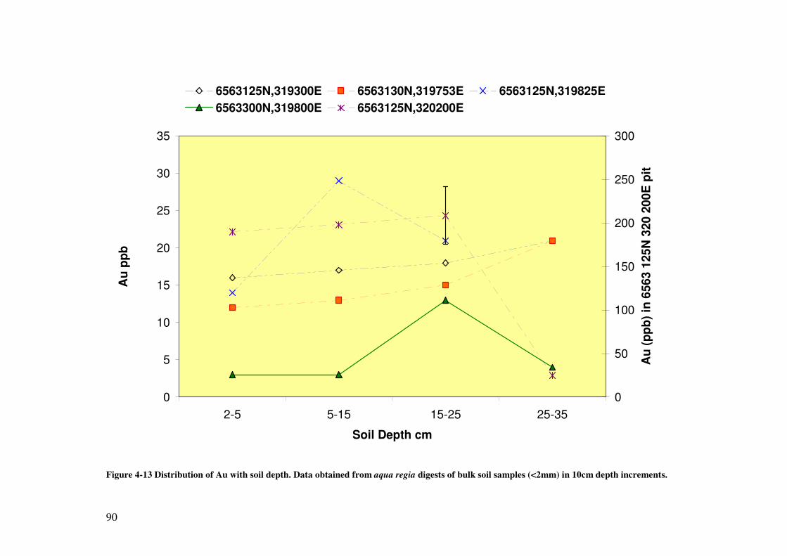
90

0

5

10

15

20

25

30

35

2-5 5-15 15-25 25-35

Soil Depth cm

Au

pp

b

0

50

100

150

200

250

300

Au

(p

pb

) in

6563 1

25N

32

0 2

00

E p

it

6563125N,319300E 6563130N,319753E 6563125N,319825E

6563300N,319800E 6563125N,320200E

Figure 4-13 Distribution of Au with soil depth. Data obtained from aqua regia digests of bulk soil samples (<2mm) in 10cm depth increments.

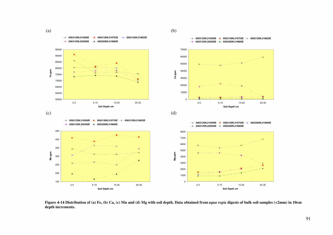
91

(a)

55000

60000

65000

70000

75000

80000

85000

90000

95000

2-5 5-15 15-25 25-35

Soil Depth cm

Fe p

pm

6563125N,319300E 6563130N,319753E 6563125N,319825E

6563125N,320200E 6563300N,319800E

(b)

0

10000

20000

30000

40000

50000

60000

70000

2-5 5-15 15-25 25-35

Soil Depth cm

Ca p

pm

6563125N,319300E 6563130N,319753E 6563125N,319825E

6563125N,320200E 6563300N,319800E

(c)

150

200

250

300

350

400

450

2-5 5-15 15-25 25-35

Soil Depth cm

Mn

pp

m

6563125N,319300E 6563130N,319753E 6563125N,319825E

6563125N,320200E 6563300N,319800E

(d)

0

1000

2000

3000

4000

5000

6000

7000

8000

2-5 5-15 15-25 25-35

Soil Depth cm

Mg

pp

m

6563125N,319300E 6563130N,319753E 6563300N,319800E

6563125N,320200E 6563300N,319800E

Figure 4-14 Distribution of (a) Fe, (b) Ca, (c) Mn and (d) Mg with soil depth. Data obtained from aqua regia digests of bulk soil samples (<2mm) in 10cm

depth increments.

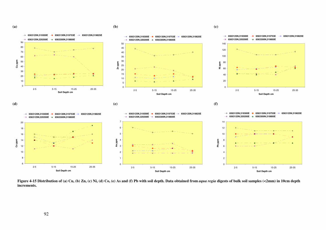
92

(a)

0

10

20

30

40

50

60

70

80

90

2-5 5-15 15-25 25-35

Soil Depth cm

Cu

pp

m

6563125N,319300E 6563130N,319753E 6563125N,319825E

6563125N,320200E 6563300N,319800E

(b)

0

5

10

15

20

25

30

35

40

45

50

2-5 5-15 15-25 25-35

Soil Depth cm

Zn

pp

m

6563125N,319300E 6563130N,319753E 6563125N,319825E

6563125N,320200E 6563300N,319800E

(c)

0

20

40

60

80

100

120

140

2-5 5-15 15-25 25-35

Soil Depth cm

Ni p

pm

6563125N,319300E 6563130N,319753E 6563125N,319825E

6563125N,320200E 6563300N,319800E

(d)

6

8

10

12

14

16

18

20

2-5 5-15 15-25 25-35

Soil Depth cm

Co

pp

m

6563125N,319300E 6563130N,319753E 6563125N,319825E

6563125N,320200E 6563300N,319800E

(e)

0

1

2

3

4

5

6

7

2-5 5-15 15-25 25-35

Soil Depth cm

As p

pm

6563125N,319300E 6563130N,319753E 6563125N,319825E

6563125N,320200E 6563300N,319800E

(f)

0

2

4

6

8

10

12

14

2-5 5-15 15-25 25-35

Soil Depth cm

Pb

pp

m

6563125N,319300E 6563130N,319753E 6563125N,319825E

6563125N,320200E 6563300N,319800E

Figure 4-15 Distribution of (a) Cu, (b) Zn, (c) Ni, (d) Co, (e) As and (f) Pb with soil depth. Data obtained from aqua regia digests of bulk soil samples (<2mm) in 10cm depth

increments.

93

4.2.4. Plant response in litter and leaf samples

Only the results of leaf and litter analyses are reported in this section because of the

small number of bark and twig samples analysed. The response in leaf and litter samples

across both transects are shown in Figure 4-16 to Figure 4-25. The same clustering of

high response ratios that were seen for the soil samples were also observed in the leaf

and litter samples at two points on the southern transect, over the pyroxenite unit at

about 319 800E and near the ultramafic/metabasalt contact at 319 850E. The strongest

responses in both plant samples were from eucalypt trees growing above the pyroxenite

lithological unit, particularly around 319 800E. At the ultramafic/metabasalt lithological

contact, high plant responses were obtained for Cd, Co, Cr and Ni. Strong responses, of

greater than 10 times background concentrations, were obtained in litter samples for Cr

(320 ppb), Pb (2175 ppb), Th (137 ppb) and U (367 ppb) at approximately 319 850E in

the pyroxenite lithological unit (southern transect). A particularly strong response in a

leaf sample was obtained for Cd at approximately 80 times background at the same

point along the southern transect in the pyroxenite (155 ppb). It is unclear if the result

obtained in this one leaf sample was spurious since the leaf samples 100 m either side of

this location were comparable to background concentrations. However, comparison

with the litter results from 100 m either side of this anomalous value shows high

responses as well and may therefore indicate true anomalism in the leaf sample. Au in

litter at 5- 6 times background was obtained from trees growing above the pyroxenite.

There were lower responses (<5 times background) overall for most elements measured

in the leaf samples except As, Cr, Ni, Th, U and Pb (>5 times background) (Figure 4-21

and Figure 4-22). There are strong responses from leaf samples for Th (20-100 ppb), U

(15-57 ppb) and Pb (50-520 ppb) from trees over the pyroxenite (Figure 4-21). As, Cr

and Ni measured in the leaf samples show enrichment in trees at the same two points

along the southern transect in the pyroxenite unit and the ultramafic/metabasalt contact.

In contrast, only Pb, measured in leaves in the trees showed enrichment in the

pyroxenite unit to the north (100-430 ppb) (Northern Transect, 6563 350N). Low

responses for all other elements were obtained for both vegetation sample types from

trees in the northern transect.

Calculated Z scores indicate a one point anomaly each for Au, As and Zn over the

pyroxenite in the litter samples (Figure 4-18 and Figure 4-19). The Z scores from litter

samples point to anomalous values for Au in the western end of the southern transect

(Figure 4-18). There are one point anomalies for Zn and Th each from the litter samples

94

in the ultramafics west of the 318 970E contact and the metabasalt between 318 970E

and 319 420E. The Z scores for leaf samples show anomalies for Ni, Cr in the

metabasalt near the ultramafic/metabasalt contact (318 970E) (Figure 4-23) and a one

point anomaly for Th in the ultramafics at the western end of the southern transect

(Figure 4-25). There are leaf anomalies for As, Cu, Cd, Th, U, Pb and Zn at various

points along the southern transect, over the pyroxenite unit (Figure 4-24 and Figure

4-25). Apart from the one point anomaly for Co in the northern transect, there were no

anomalies for any other element detected in the leaves over the pyroxenite in the

northern transect. Similarly weak anomalies were obtained for Cr, Ni, As, Co, Zn, Pb,

Th and U in the litter samples taken from the northern transect.

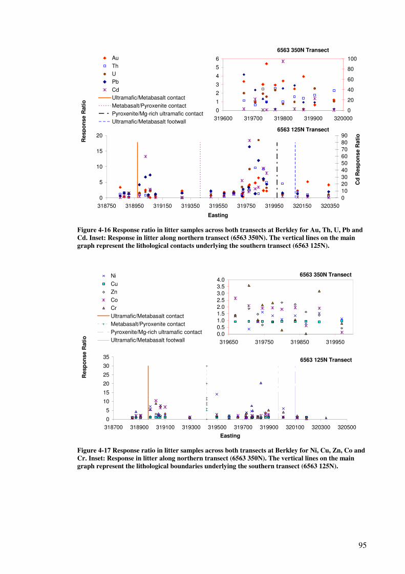
95

6563 125N Transect

0

5

10

15

20

318750 318950 319150 319350 319550 319750 319950 320150 320350

Easting

0

10

20

30

40

50

60

70

80

90

Au

Th

U

Pb

Cd





6563 350N Transect

0

1

2

3

4

5

6

319600 319700 319800 319900 320000

0

20

40

60

80

100

Re

sp

on

se

Ra

tio

Cd

Res

po

ns

e R

ati

o

Figure 4-16 Response ratio in litter samples across both transects at Berkley for Au, Th, U, Pb and

Cd. Inset: Response in litter along northern transect (6563 350N). The vertical lines on the main

graph represent the lithological contacts underlying the southern transect (6563 125N).

6563 125N Transect

0

5

10

15

20

25

30

35

318700 318900 319100 319300 319500 319700 319900 320100 320300 320500

Easting

Re

sp

on

se

Ra

tio

Ni

Cu

Zn

Co

Cr





6563 350N Transect

0.0

0.5

1.0

1.5

2.0

2.5

3.0

3.5

4.0

319650 319750 319850 319950

Figure 4-17 Response ratio in litter samples across both transects at Berkley for Ni, Cu, Zn, Co and

Cr. Inset: Response in litter along northern transect (6563 350N). The vertical lines on the main

graph represent the lithological boundaries underlying the southern transect (6563 125N).

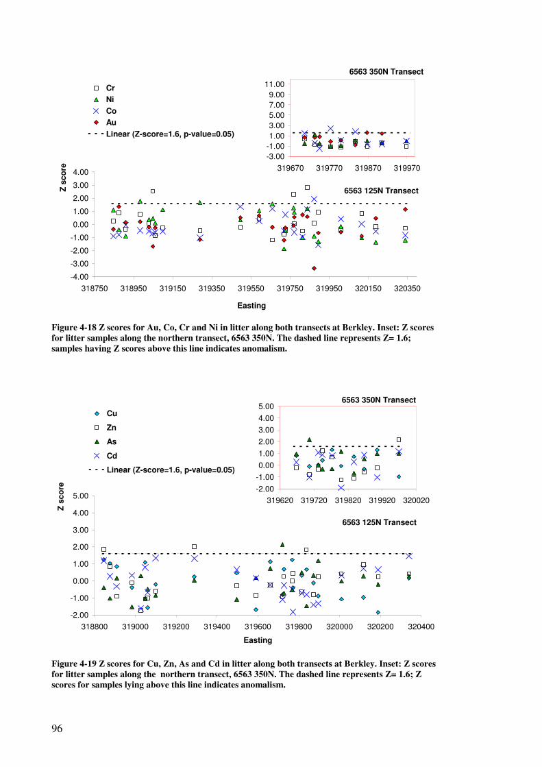
96

6563 125N Transect

-4.00

-3.00

-2.00

-1.00

0.00

1.00

2.00

3.00

4.00

318750 318950 319150 319350 319550 319750 319950 320150 320350

Easting

Z s

co

re

Cr

Ni

Co

Au

Linear (Z-score=1.6, p-value=0.05)

6563 350N Transect

-3.00

-1.00

1.00

3.00

5.00

7.00

9.00

11.00

319670 319770 319870 319970

Figure 4-18 Z scores for Au, Co, Cr and Ni in litter along both transects at Berkley. Inset: Z scores

for litter samples along the northern transect, 6563 350N. The dashed line represents Z= 1.6;

samples having Z scores above this line indicates anomalism.

6563 125N Transect

-2.00

-1.00

0.00

1.00

2.00

3.00

4.00

5.00

318800 319000 319200 319400 319600 319800 320000 320200 320400

Easting

Z s

co

re

Cu

Zn

As

Cd


6563 350N Transect

-2.00

-1.00

0.00

1.00

2.00

3.00

4.00

5.00

319620 319720 319820 319920 320020

Figure 4-19 Z scores for Cu, Zn, As and Cd in litter along both transects at Berkley. Inset: Z scores

for litter samples along the northern transect, 6563 350N. The dashed line represents Z= 1.6; Z

scores for samples lying above this line indicates anomalism.

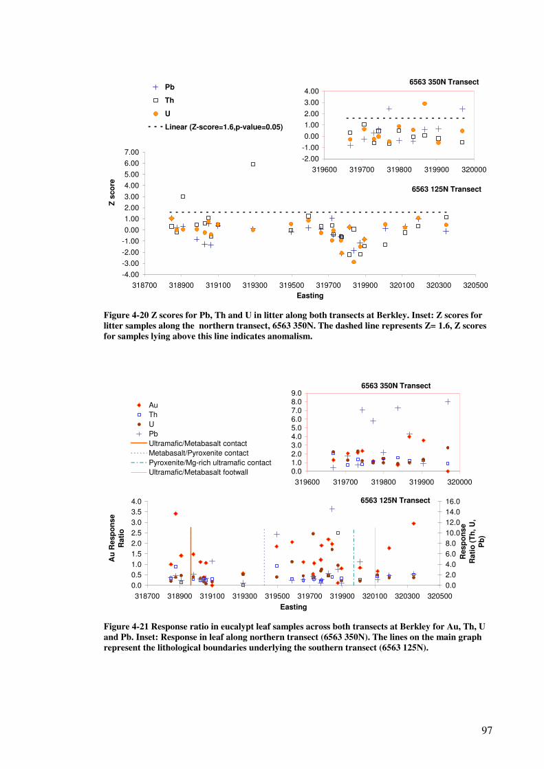
97

6563 125N Transect

-4.00

-3.00

-2.00

-1.00

0.00

1.00

2.00

3.00

4.00

5.00

6.00

7.00

318700 318900 319100 319300 319500 319700 319900 320100 320300 320500

Easting

Z s

co

re

Pb

Th

U

Linear (Z-score=1.6,p-value=0.05)

6563 350N Transect

-2.00

-1.00

0.00

1.00

2.00

3.00

4.00

319600 319700 319800 319900 320000

Figure 4-20 Z scores for Pb, Th and U in litter along both transects at Berkley. Inset: Z scores for

litter samples along the northern transect, 6563 350N. The dashed line represents Z= 1.6, Z scores

for samples lying above this line indicates anomalism.

6563 125N Transect

0.0

0.5

1.0

1.5

2.0

2.5

3.0

3.5

4.0

318700 318900 319100 319300 319500 319700 319900 320100 320300 320500

Easting

Au

Re

sp

on

se

Ra

tio

0.0

2.0

4.0

6.0

8.0

10.0

12.0

14.0

16.0

Res

po

ns

e

Ra

tio

(T

h,

U,

Pb

)

Au

Th

U

Pb





6563 350N Transect

0.01.02.03.04.05.06.07.08.09.0

319600 319700 319800 319900 320000

Figure 4-21 Response ratio in eucalypt leaf samples across both transects at Berkley for Au, Th, U

and Pb. Inset: Response in leaf along northern transect (6563 350N). The lines on the main graph

represent the lithological boundaries underlying the southern transect (6563 125N).

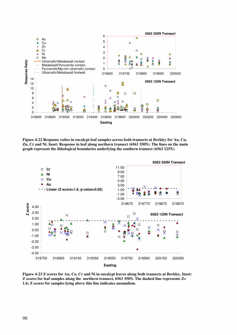
98

6563 125N Transect

0

2

4

6

8

10

12

14

318600 318800 319000 319200 319400 319600 319800 320000 320200 320400 320600

Easting

Re

sp

on

se R

ati

o

AsCuZnCrNiMnUltramafic/Metabasalt contactMetabasalt/Pyroxenite contactPyroxenite/Mg-rich ultramafic contactUltramafic/Metabasalt footwall

6563 350N Transect

0

1

2

3

4

5

6

319600 319700 319800 319900 320000

Figure 4-22 Response ratios in eucalypt leaf samples across both transects at Berkley for Au, Cu,

Zn, Cr and Ni. Inset: Response in leaf along northern transect (6563 350N). The lines on the main

graph represent the lithological boundaries underlying the southern transect (6563 125N).

6563 125N Transect

-4.00

-3.00

-2.00

-1.00

0.00

1.00

2.00

3.00

4.00

318750 318950 319150 319350 319550 319750 319950 320150 320350

Easting

Z s

co

re

Cr

Ni

Co

Au


6563 350N Transect

-3.00

-1.00

1.00

3.00

5.00

7.00

9.00

11.00

319670 319770 319870 319970

Figure 4-23 Z scores for Au, Co, Cr and Ni in eucalypt leaves along both transects at Berkley. Inset:

Z scores for leaf samples along the northern transect, 6563 350N. The dashed line represents Z=

1.6; Z scores for samples lying above this line indicates anomalism.

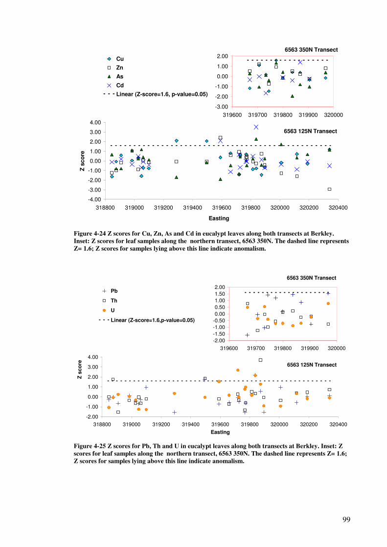
99

6563 125N Transect

-4.00

-3.00

-2.00

-1.00

0.00

1.00

2.00

3.00

4.00

318800 319000 319200 319400 319600 319800 320000 320200 320400

Easting

Z s

co

re

Cu

Zn

As

Cd


6563 350N Transect

-3.00

-2.00

-1.00

0.00

1.00

2.00

319600 319700 319800 319900 320000

Figure 4-24 Z scores for Cu, Zn, As and Cd in eucalypt leaves along both transects at Berkley.

Inset: Z scores for leaf samples along the northern transect, 6563 350N. The dashed line represents

Z= 1.6; Z scores for samples lying above this line indicate anomalism.

6563 125N Transect

-2.00

-1.00

0.00

1.00

2.00

3.00

4.00

318800 319000 319200 319400 319600 319800 320000 320200 320400

Easting

Z s

co

re

Pb

Th

U

Linear (Z-score=1.6,p-value=0.05)

6563 350N Transect

-2.00

-1.50

-1.00

-0.50

0.00

0.50

1.00

1.50

2.00

319600 319700 319800 319900 320000

Figure 4-25 Z scores for Pb, Th and U in eucalypt leaves along both transects at Berkley. Inset: Z

scores for leaf samples along the northern transect, 6563 350N. The dashed line represents Z= 1.6;

Z scores for samples lying above this line indicate anomalism.

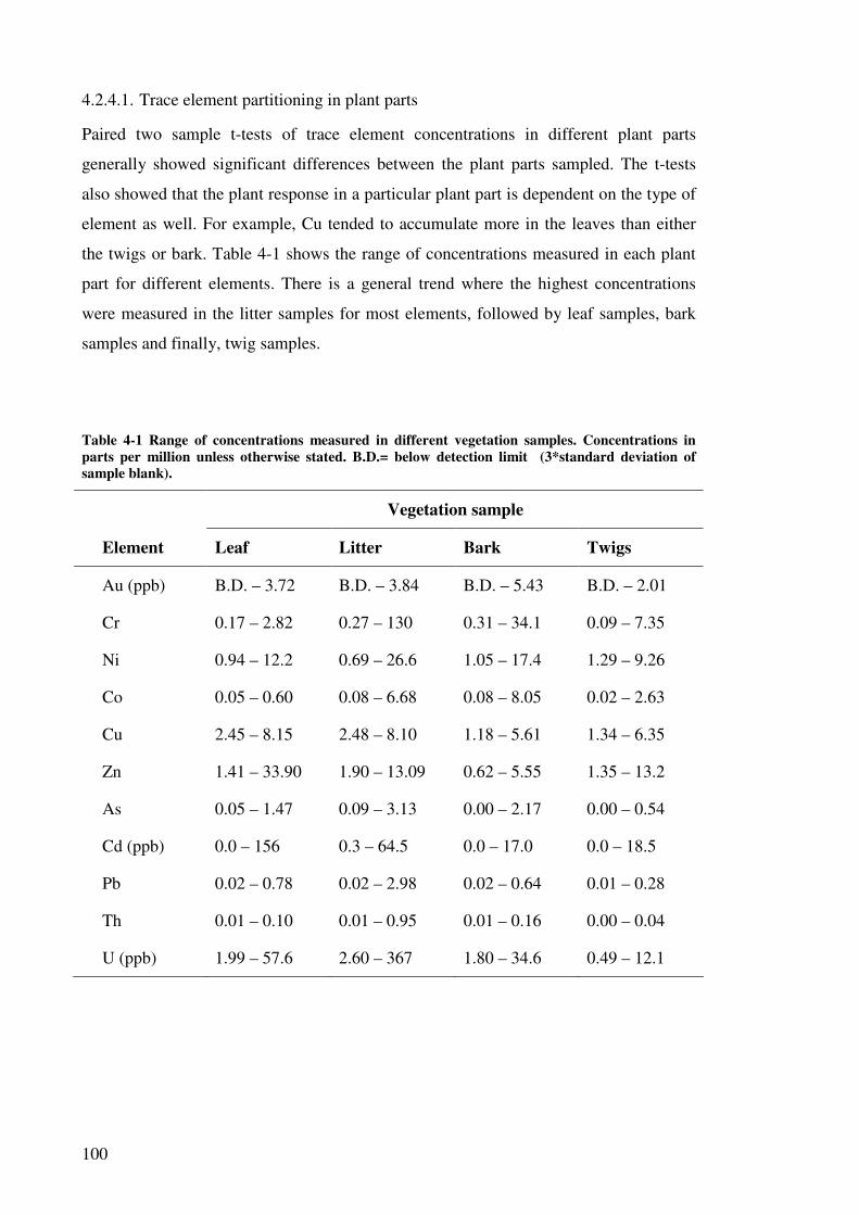
100

4.2.4.1. Trace element partitioning in plant parts

Paired two sample t-tests of trace element concentrations in different plant parts

generally showed significant differences between the plant parts sampled. The t-tests

also showed that the plant response in a particular plant part is dependent on the type of

element as well. For example, Cu tended to accumulate more in the leaves than either

the twigs or bark. Table 4-1 shows the range of concentrations measured in each plant

part for different elements. There is a general trend where the highest concentrations

were measured in the litter samples for most elements, followed by leaf samples, bark

samples and finally, twig samples.

Table 4-1 Range of concentrations measured in different vegetation samples. Concentrations in

parts per million unless otherwise stated. B.D.= below detection limit (3*standard deviation of

sample blank).

Vegetation sample

Element Leaf Litter Bark Twigs

Au (ppb) B.D. – 3.72 B.D. – 3.84 B.D. – 5.43 B.D. – 2.01

Cr 0.17 – 2.82 0.27 – 130 0.31 – 34.1 0.09 – 7.35

Ni 0.94 – 12.2 0.69 – 26.6 1.05 – 17.4 1.29 – 9.26

Co 0.05 – 0.60 0.08 – 6.68 0.08 – 8.05 0.02 – 2.63

Cu 2.45 – 8.15 2.48 – 8.10 1.18 – 5.61 1.34 – 6.35

Zn 1.41 – 33.90 1.90 – 13.09 0.62 – 5.55 1.35 – 13.2

As 0.05 – 1.47 0.09 – 3.13 0.00 – 2.17 0.00 – 0.54

Cd (ppb) 0.0 – 156 0.3 – 64.5 0.0 – 17.0 0.0 – 18.5

Pb 0.02 – 0.78 0.02 – 2.98 0.02 – 0.64 0.01 – 0.28

Th 0.01 – 0.10 0.01 – 0.95 0.01 – 0.16 0.00 – 0.04

U (ppb) 1.99 – 57.6 2.60 – 367 1.80 – 34.6 0.49 – 12.1

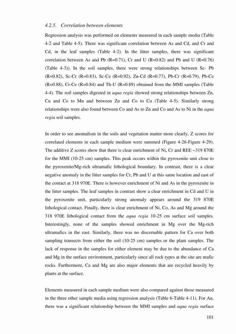
101

4.2.5. Correlation between elements

Regression analysis was performed on elements measured in each sample media (Table

4-2 and Table 4-5). There was significant correlation between As and Cd, and Cr and

Cd, in the leaf samples (Table 4-2). In the litter samples, there was significant

correlation between As and Pb (R=0.71), Cr and U (R=0.82) and Pb and U (R=0.76)

(Table 4-3)). In the soil samples, there were strong relationships between Sc- Pb

(R=0.82), Sc-Cr (R=0.83), Sc-Ce (R=0.92), Zn-Cd (R=0.77), Pb-Cr (R=0.79), Pb-Ce

(R=0.88), Cr-Ce (R=0.84) and Th-U (R=0.89) obtained from the MMI samples (Table

4-4). The soil samples digested in aqua regia showed strong relationships between Zn,

Cu and Co to Mn and between Zn and Co to Cu (Table 4-5). Similarly strong

relationships were also found between Co and As to Zn and Co and As to Ni in the aqua

regia soil samples.

In order to see anomalism in the soils and vegetation matter more clearly, Z scores for

correlated elements in each sample medium were summed (Figure 4-26-Figure 4-29).

The additive Z scores show that there is clear enrichment of Ni, Cr and REE ~319 870E

for the MMI (10-25 cm) samples. This peak occurs within the pyroxenite unit close to

the pyroxenite/Mg-rich ultramafic lithological boundary. In contrast, there is a clear

negative anomaly in the litter samples for Cr, Pb and U at this same location and east of

the contact at 318 970E. There is however enrichment of Ni and As in the pyroxenite in

the litter samples. The leaf samples in contrast show a clear enrichment in Cd and U in

the pyroxenite unit, particularly strong anomaly appears around the 319 870E

lithological contact. Finally, there is clear enrichment of Ni, Co, As and Mg around the

318 970E lithological contact from the aqua regia 10-25 cm surface soil samples.

Interestingly, none of the samples showed enrichment in Mg over the Mg-rich

ultramafics in the east. Similarly, there was no discernable pattern for Ca over both

sampling transects from either the soil (10-25 cm) samples or the plant samples. The

lack of response in the samples for either element may be due to the abundance of Ca

and Mg in the surface environment, particularly since all rock types at the site are mafic

rocks. Furthermore, Ca and Mg are also major elements that are recycled heavily by

plants at the surface.

Elements measured in each sample medium were also compared against those measured

in the three other sample media using regression analysis (Table 6-Table 4-11). For Au,

there was a significant relationship between the MMI samples and aqua regia surface

102

soil samples (10-25cm). Elements that showed significant correlation between the MMI

and aqua regia soil samples were also found for Ca, Cu, Mg and Ni. Between the leaf

and MMI soil samples, Fe was significantly and negatively correlated while Mn was

positively correlated. Between litter and MMI soil samples, Mg and Mn were positively

correlated. Only Ni showed a significant positive correlation between the aqua regia

digested soils and the leaves, whereas the litter showed Co and Ni to be significantly

correlated to the aqua regia digested soils. Finally, Th, U, Ca, Mg and Mn showed a

positive correlation between the leaf and litter samples. The types of elements that are

positively correlated between the types of sample media appear to be readily

bioavailable and abundant.

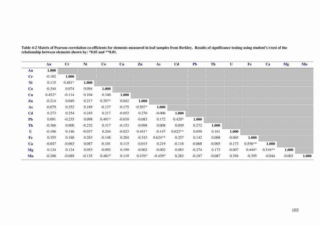
103

Table 4-2 Matrix of Pearson correlation co-efficients for elements measured in leaf samples from Berkley. Results of significance testing using student’s t-test of the

relationship between elements shown by: *0.05 and **0.01.

Au Cr Ni Co Cu Zn As Cd Pb Th U Fe Ca Mg Mn

Au 1.000

Cr -0.182 1.000

Ni 0.115 0.481* 1.000

Co -0.344 0.074 0.094 1.000

Cu 0.452* -0.114 0.104 0.340 1.000

Zn -0.214 0.049 0.217 0.397* 0.042 1.000

As -0.079 0.352 0.189 -0.137 -0.175 -0.507* 1.000

Cd 0.273 0.254 0.245 0.217 -0.052 0.270 -0.006 1.000

Pb 0.091 -0.235 0.098 0.401* -0.010 -0.083 0.172 0.420* 1.000

Th -0.366 0.000 -0.232 0.317 -0.153 -0.098 0.008 0.049 0.272 1.000

U -0.106 0.146 -0.037 0.244 -0.023 0.441* -0.147 0.622** 0.050 0.161 1.000

Fe 0.355 0.180 0.283 -0.148 0.204 -0.343 0.624** 0.257 0.142 0.008 -0.065 1.000

Ca -0.047 -0.063 0.087 -0.101 0.115 -0.015 0.219 -0.118 -0.068 -0.005 -0.173 0.556** 1.000

Mg 0.124 0.124 0.053 -0.092 0.199 -0.002 -0.002 0.083 -0.274 0.175 -0.007 0.444* 0.516** 1.000

Mn -0.208 -0.089 -0.135 0.481* 0.119 0.476* -0.439* 0.283 -0.187 -0.087 0.394 -0.395 -0.044 -0.003 1.000

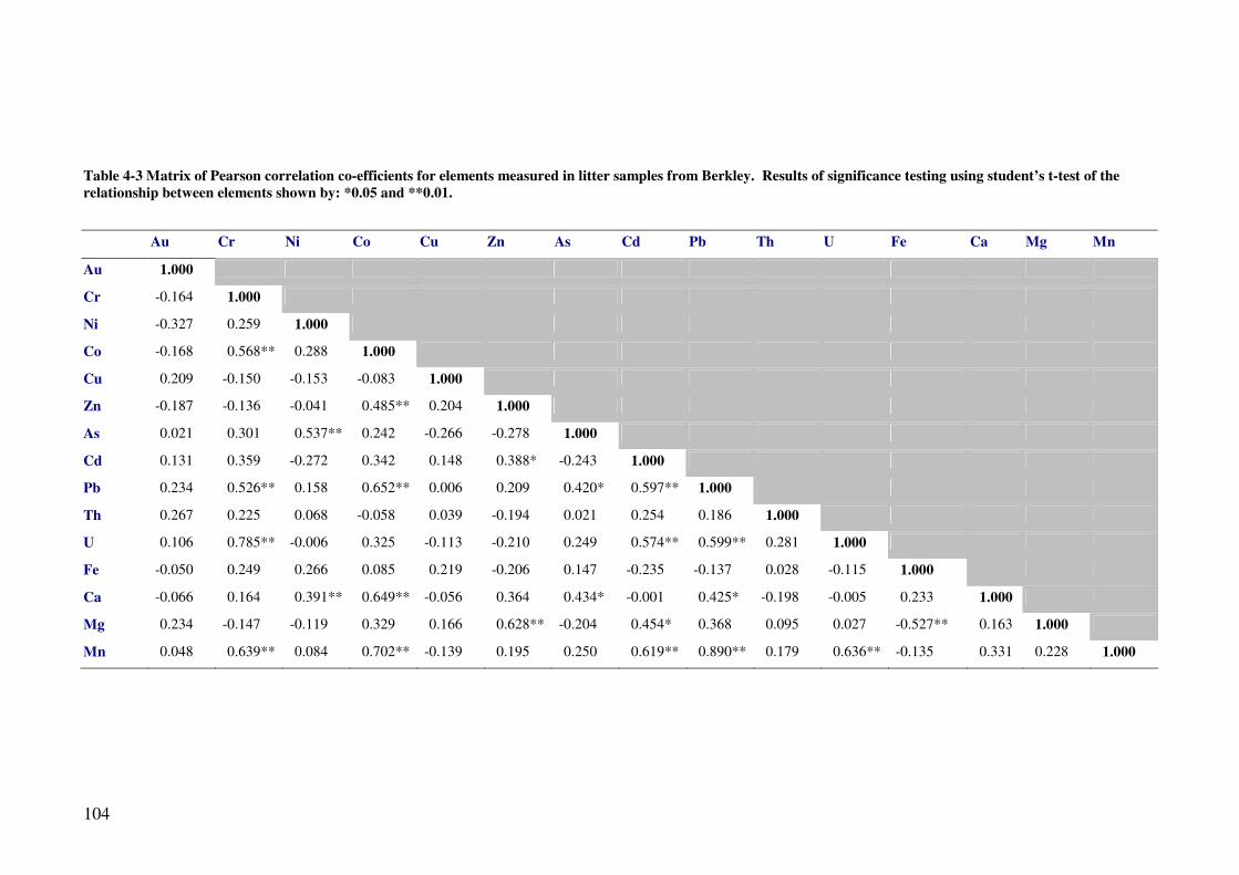
104

Table 4-3 Matrix of Pearson correlation co-efficients for elements measured in litter samples from Berkley. Results of significance testing using student’s t-test of the

relationship between elements shown by: *0.05 and **0.01.

Au Cr Ni Co Cu Zn As Cd Pb Th U Fe Ca Mg Mn

Au 1.000

Cr -0.164 1.000

Ni -0.327 0.259 1.000

Co -0.168 0.568** 0.288 1.000

Cu 0.209 -0.150 -0.153 -0.083 1.000

Zn -0.187 -0.136 -0.041 0.485** 0.204 1.000

As 0.021 0.301 0.537** 0.242 -0.266 -0.278 1.000

Cd 0.131 0.359 -0.272 0.342 0.148 0.388* -0.243 1.000

Pb 0.234 0.526** 0.158 0.652** 0.006 0.209 0.420* 0.597** 1.000

Th 0.267 0.225 0.068 -0.058 0.039 -0.194 0.021 0.254 0.186 1.000

U 0.106 0.785** -0.006 0.325 -0.113 -0.210 0.249 0.574** 0.599** 0.281 1.000

Fe -0.050 0.249 0.266 0.085 0.219 -0.206 0.147 -0.235 -0.137 0.028 -0.115 1.000

Ca -0.066 0.164 0.391** 0.649** -0.056 0.364 0.434* -0.001 0.425* -0.198 -0.005 0.233 1.000

Mg 0.234 -0.147 -0.119 0.329 0.166 0.628** -0.204 0.454* 0.368 0.095 0.027 -0.527** 0.163 1.000

Mn 0.048 0.639** 0.084 0.702** -0.139 0.195 0.250 0.619** 0.890** 0.179 0.636** -0.135 0.331 0.228 1.000

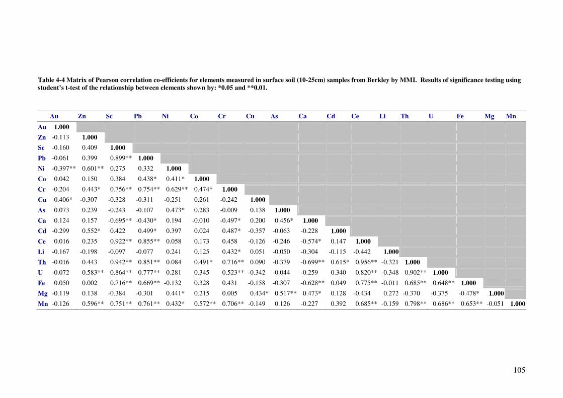
105

Table 4-4 Matrix of Pearson correlation co-efficients for elements measured in surface soil (10-25cm) samples from Berkley by MMI. Results of significance testing using

student’s t-test of the relationship between elements shown by: *0.05 and **0.01.

Au Zn Sc Pb Ni Co Cr Cu As Ca Cd Ce Li Th U Fe Mg Mn

Au 1.000

Zn -0.113 1.000

Sc -0.160 0.409 1.000

Pb -0.061 0.399 0.899** 1.000

Ni -0.397** 0.601** 0.275 0.332 1.000

Co 0.042 0.150 0.384 0.438* 0.411* 1.000

Cr -0.204 0.443* 0.756** 0.754** 0.629** 0.474* 1.000

Cu 0.406* -0.307 -0.328 -0.311 -0.251 0.261 -0.242 1.000

As 0.073 0.239 -0.243 -0.107 0.473* 0.283 -0.009 0.138 1.000

Ca 0.124 0.157 -0.695** -0.430* 0.194 -0.010 -0.497* 0.200 0.456* 1.000

Cd -0.299 0.552* 0.422 0.499* 0.397 0.024 0.487* -0.357 -0.063 -0.228 1.000

Ce 0.016 0.235 0.922** 0.855** 0.058 0.173 0.458 -0.126 -0.246 -0.574* 0.147 1.000

Li -0.167 -0.198 -0.097 -0.077 0.241 0.125 0.432* 0.051 -0.050 -0.304 -0.115 -0.442 1.000

Th -0.016 0.443 0.942** 0.851** 0.084 0.491* 0.716** 0.090 -0.379 -0.699** 0.615* 0.956** -0.321 1.000

U -0.072 0.583** 0.864** 0.777** 0.281 0.345 0.523** -0.342 -0.044 -0.259 0.340 0.820** -0.348 0.902** 1.000

Fe 0.050 0.002 0.716** 0.669** -0.132 0.328 0.431 -0.158 -0.307 -0.628** 0.049 0.775** -0.011 0.685** 0.648** 1.000

Mg -0.119 0.138 -0.384 -0.301 0.441* 0.215 0.005 0.434* 0.517** 0.473* 0.128 -0.434 0.272 -0.370 -0.375 -0.478* 1.000

Mn -0.126 0.596** 0.751** 0.761** 0.432* 0.572** 0.706** -0.149 0.126 -0.227 0.392 0.685** -0.159 0.798** 0.686** 0.653** -0.051 1.000

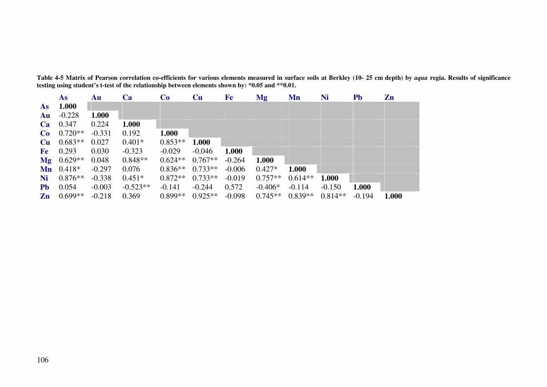
106

Table 4-5 Matrix of Pearson correlation co-efficients for various elements measured in surface soils at Berkley (10- 25 cm depth) by aqua regia. Results of significance

testing using student’s t-test of the relationship between elements shown by: *0.05 and **0.01.

As Au Ca Co Cu Fe Mg Mn Ni Pb Zn

As 1.000

Au -0.228 1.000

Ca 0.347 0.224 1.000

Co 0.720** -0.331 0.192 1.000

Cu 0.683** 0.027 0.401* 0.853** 1.000

Fe 0.293 0.030 -0.323 -0.029 -0.046 1.000

Mg 0.629** 0.048 0.848** 0.624** 0.767** -0.264 1.000

Mn 0.418* -0.297 0.076 0.836** 0.733** -0.006 0.427* 1.000

Ni 0.876** -0.338 0.451* 0.872** 0.733** -0.019 0.757** 0.614** 1.000

Pb 0.054 -0.003 -0.523** -0.141 -0.244 0.572 -0.406* -0.114 -0.150 1.000

Zn 0.699** -0.218 0.369 0.899** 0.925** -0.098 0.745** 0.839** 0.814** -0.194 1.000

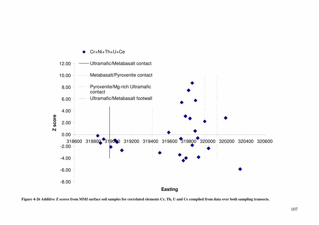
107

-8.00

-6.00

-4.00

-2.00

0.00

2.00

4.00

6.00

8.00

10.00

12.00

318600 318800 319000 319200 319400 319600 319800 320000 320200 320400 320600

Easting

Z s

co

reCr+Ni+Th+U+Ce



Pyroxenite/Mg-rich Ultramaficcontact


Figure 4-26 Additive Z scores from MMI surface soil samples for correlated elements Cr, Th, U and Ce compiled from data over both sampling transects.

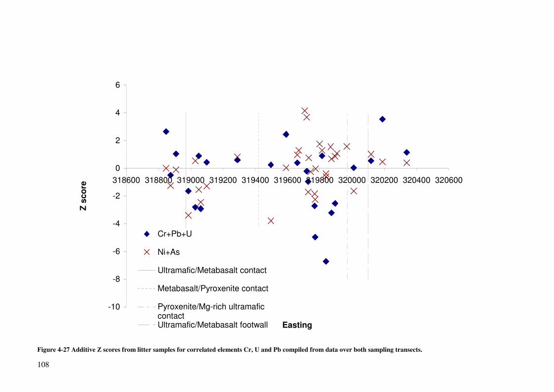
108

-10

-8

-6

-4

-2

0

2

4

6

318600 318800 319000 319200 319400 319600 319800 320000 320200 320400 320600

Easting

Z s

co

re

Cr+Pb+U

Ni+As



Pyroxenite/Mg-rich ultramaficcontactUltramafic/Metabasalt footwall

Figure 4-27 Additive Z scores from litter samples for correlated elements Cr, U and Pb compiled from data over both sampling transects.

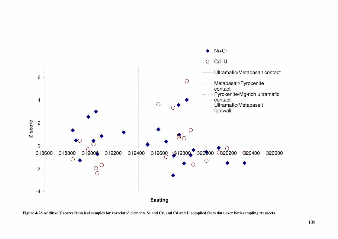
109

-4

-2

0

2

4

6

318600 318800 319000 319200 319400 319600 319800 320000 320200 320400 320600

Easting

Z s

co

re

Ni+Cr

Cd+U


Metabasalt/PyroxenitecontactPyroxenite/Mg-rich ultramaficcontactUltramafic/Metabasaltfootwall

Figure 4-28 Additive Z scores from leaf samples for correlated elements Ni and Cr, and Cd and U compiled from data over both sampling transects.

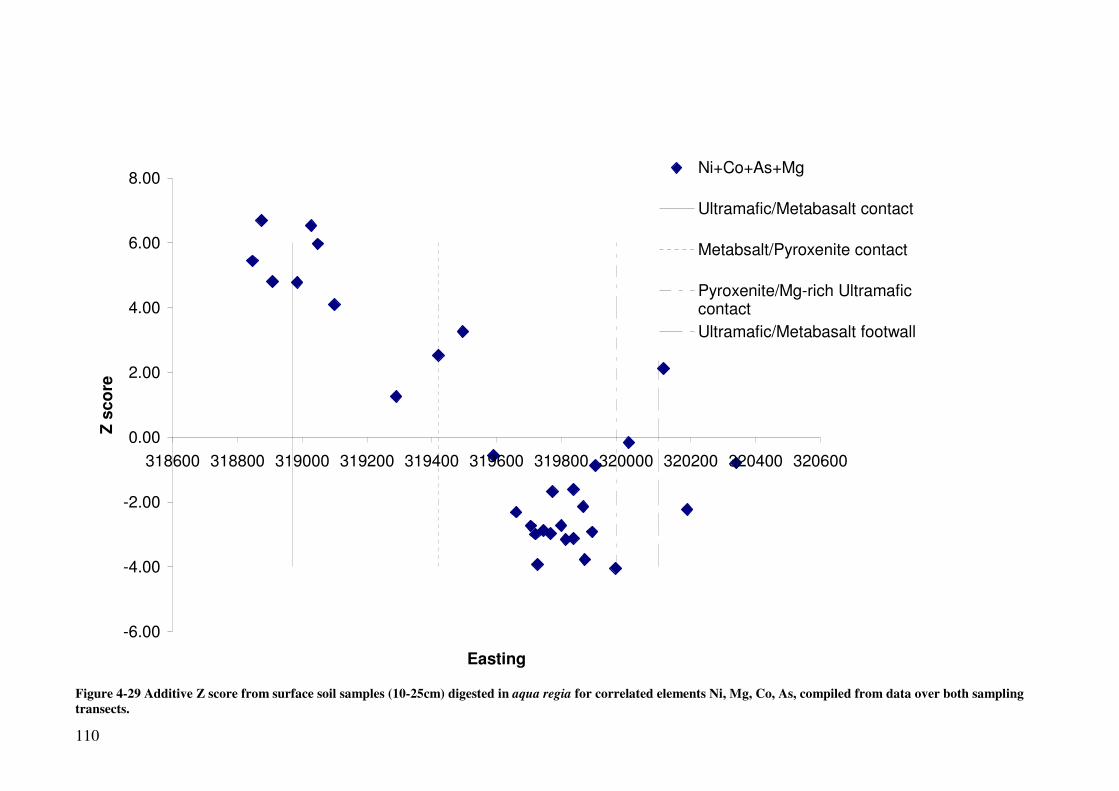
110

-6.00

-4.00

-2.00

0.00

2.00

4.00

6.00

8.00

318600 318800 319000 319200 319400 319600 319800 320000 320200 320400 320600

Easting

Z s

co

re

Ni+Co+As+Mg


Metabsalt/Pyroxenite contact

Pyroxenite/Mg-rich Ultramaficcontact


Figure 4-29 Additive Z score from surface soil samples (10-25cm) digested in aqua regia for correlated elements Ni, Mg, Co, As, compiled from data over both sampling

transects.

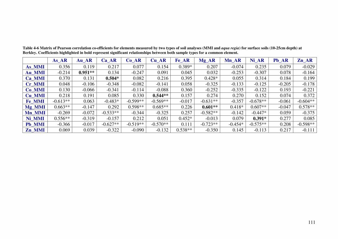
111

Table 4-6 Matrix of Pearson correlation co-efficients for elements measured by two types of soil analyses (MMI and aqua regia) for surface soils (10-25cm depth) at

Berkley. Coefficients highlighted in bold represent significant relationships between both sample types for a common element.

As_AR Au_AR Ca_AR Co_AR Cu_AR Fe_AR Mg_AR Mn_AR Ni_AR Pb_AR Zn_AR

As_MMI 0.356 0.119 0.217 0.077 0.154 0.389* 0.207 -0.074 0.235 0.079 -0.029

Au_MMI -0.214 0.951** 0.134 -0.247 0.091 0.045 0.032 -0.253 -0.307 0.078 -0.164

Ca_MMI 0.370 0.131 0.504* 0.082 0.216 0.395 0.428* 0.055 0.314 0.184 0.199

Cr_MMI 0.048 -0.106 -0.348 -0.082 -0.141 0.058 -0.325 -0.133 -0.125 -0.205 -0.178

Co_MMI 0.130 -0.066 -0.341 -0.114 -0.088 0.360 -0.252 -0.335 -0.122 0.193 -0.221

Cu_MMI 0.218 0.191 0.085 0.330 0.544** 0.157 0.274 0.270 0.152 0.074 0.372

Fe_MMI -0.613** 0.063 -0.483* -0.599** -0.569** -0.017 -0.631** -0.357 -0.678** -0.061 -0.604**

Mg_MMI 0.663** -0.147 0.292 0.598** 0.685** 0.226 0.601** 0.418* 0.607** -0.047 0.578**

Mn_MMI -0.269 -0.072 -0.533** -0.344 -0.325 0.257 -0.582** -0.142 -0.447* 0.059 -0.375

Ni_MMI 0.556** -0.319 -0.157 0.212 0.051 0.452* -0.013 0.079 0.391* 0.277 0.085

Pb_MMI -0.366 -0.017 -0.627** -0.519** -0.570** 0.111 -0.723** -0.454* -0.575** 0.208 -0.598**

Zn_MMI 0.069 0.039 -0.322 -0.090 -0.132 0.538** -0.350 0.145 -0.113 0.217 -0.111

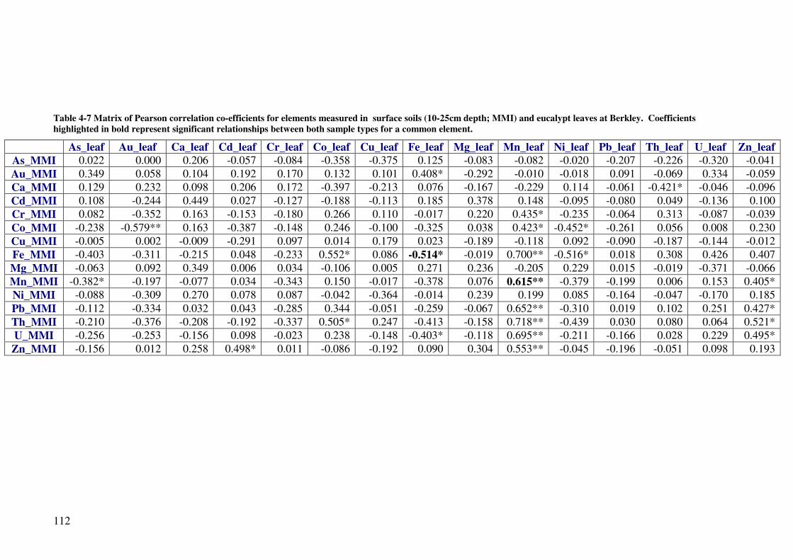
112

Table 4-7 Matrix of Pearson correlation co-efficients for elements measured in surface soils (10-25cm depth; MMI) and eucalypt leaves at Berkley. Coefficients

highlighted in bold represent significant relationships between both sample types for a common element.

As_leaf Au_leaf Ca_leaf Cd_leaf Cr_leaf Co_leaf Cu_leaf Fe_leaf Mg_leaf Mn_leaf Ni_leaf Pb_leaf Th_leaf U_leaf Zn_leaf

As_MMI 0.022 0.000 0.206 -0.057 -0.084 -0.358 -0.375 0.125 -0.083 -0.082 -0.020 -0.207 -0.226 -0.320 -0.041

Au_MMI 0.349 0.058 0.104 0.192 0.170 0.132 0.101 0.408* -0.292 -0.010 -0.018 0.091 -0.069 0.334 -0.059

Ca_MMI 0.129 0.232 0.098 0.206 0.172 -0.397 -0.213 0.076 -0.167 -0.229 0.114 -0.061 -0.421* -0.046 -0.096

Cd_MMI 0.108 -0.244 0.449 0.027 -0.127 -0.188 -0.113 0.185 0.378 0.148 -0.095 -0.080 0.049 -0.136 0.100

Cr_MMI 0.082 -0.352 0.163 -0.153 -0.180 0.266 0.110 -0.017 0.220 0.435* -0.235 -0.064 0.313 -0.087 -0.039

Co_MMI -0.238 -0.579** 0.163 -0.387 -0.148 0.246 -0.100 -0.325 0.038 0.423* -0.452* -0.261 0.056 0.008 0.230

Cu_MMI -0.005 0.002 -0.009 -0.291 0.097 0.014 0.179 0.023 -0.189 -0.118 0.092 -0.090 -0.187 -0.144 -0.012

Fe_MMI -0.403 -0.311 -0.215 0.048 -0.233 0.552* 0.086 -0.514* -0.019 0.700** -0.516* 0.018 0.308 0.426 0.407

Mg_MMI -0.063 0.092 0.349 0.006 0.034 -0.106 0.005 0.271 0.236 -0.205 0.229 0.015 -0.019 -0.371 -0.066

Mn_MMI -0.382* -0.197 -0.077 0.034 -0.343 0.150 -0.017 -0.378 0.076 0.615** -0.379 -0.199 0.006 0.153 0.405*

Ni_MMI -0.088 -0.309 0.270 0.078 0.087 -0.042 -0.364 -0.014 0.239 0.199 0.085 -0.164 -0.047 -0.170 0.185

Pb_MMI -0.112 -0.334 0.032 0.043 -0.285 0.344 -0.051 -0.259 -0.067 0.652** -0.310 0.019 0.102 0.251 0.427*

Th_MMI -0.210 -0.376 -0.208 -0.192 -0.337 0.505* 0.247 -0.413 -0.158 0.718** -0.439 0.030 0.080 0.064 0.521*

U_MMI -0.256 -0.253 -0.156 0.098 -0.023 0.238 -0.148 -0.403* -0.118 0.695** -0.211 -0.166 0.028 0.229 0.495*

Zn_MMI -0.156 0.012 0.258 0.498* 0.011 -0.086 -0.192 0.090 0.304 0.553** -0.045 -0.196 -0.051 0.098 0.193

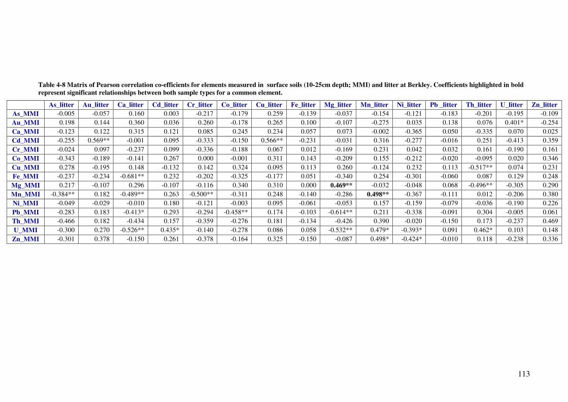
113

Table 4-8 Matrix of Pearson correlation co-efficients for elements measured in surface soils (10-25cm depth; MMI) and litter at Berkley. Coefficients highlighted in bold

represent significant relationships between both sample types for a common element.

As_litter Au_litter Ca_litter Cd_litter Cr_litter Co_litter Cu_litter Fe_litter Mg_litter Mn_litter Ni_litter Pb _litter Th_litter U_litter Zn_litter

As_MMI -0.005 -0.057 0.160 0.003 -0.217 -0.179 0.259 -0.139 -0.037 -0.154 -0.121 -0.183 -0.201 -0.195 -0.109

Au_MMI 0.198 0.144 0.360 0.036 0.260 -0.178 0.265 0.100 -0.107 -0.275 0.035 0.138 0.076 0.401* -0.254

Ca_MMI -0.123 0.122 0.315 0.121 0.085 0.245 0.234 0.057 0.073 -0.002 -0.365 0.050 -0.335 0.070 0.025

Cd_MMI -0.255 0.569** -0.001 0.095 -0.333 -0.150 0.566** -0.231 -0.031 0.316 -0.277 -0.016 0.251 -0.413 0.359

Cr_MMI -0.024 0.097 -0.237 0.099 -0.336 -0.188 0.067 0.012 -0.169 0.231 0.042 0.032 0.161 -0.190 0.161

Co_MMI -0.343 -0.189 -0.141 0.267 0.000 -0.001 0.311 0.143 -0.209 0.155 -0.212 -0.020 -0.095 0.020 0.346

Cu_MMI 0.278 -0.195 0.148 -0.132 0.142 0.324 0.095 0.113 0.260 -0.124 0.232 0.113 -0.517** 0.074 0.231

Fe_MMI -0.237 -0.234 -0.681** 0.232 -0.202 -0.325 -0.177 0.051 -0.340 0.254 -0.301 -0.060 0.087 0.129 0.248

Mg_MMI 0.217 -0.107 0.296 -0.107 -0.116 0.340 0.310 0.000 0.469** -0.032 -0.048 0.068 -0.496** -0.305 0.290

Mn_MMI -0.384** 0.182 -0.489** 0.263 -0.500** -0.311 0.248 -0.140 -0.286 0.498** -0.367 -0.111 0.012 -0.206 0.380

Ni_MMI -0.049 -0.029 -0.010 0.180 -0.121 -0.003 0.095 -0.061 -0.053 0.157 -0.159 -0.079 -0.036 -0.190 0.226

Pb_MMI -0.283 0.183 -0.413* 0.293 -0.294 -0.458** 0.174 -0.103 -0.614** 0.211 -0.338 -0.091 0.304 -0.005 0.061

Th_MMI -0.466 0.182 -0.434 0.157 -0.359 -0.276 0.181 -0.134 -0.426 0.390 -0.020 -0.150 0.173 -0.237 0.469

U_MMI -0.300 0.270 -0.526** 0.435* -0.140 -0.278 0.086 0.058 -0.532** 0.479* -0.393* 0.091 0.462* 0.103 0.148

Zn_MMI -0.301 0.378 -0.150 0.261 -0.378 -0.164 0.325 -0.150 -0.087 0.498* -0.424* -0.010 0.118 -0.238 0.336

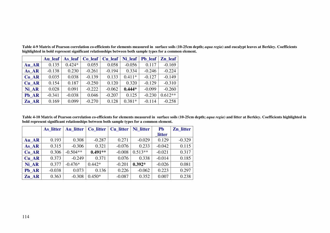
114

Table 4-9 Matrix of Pearson correlation co-efficients for elements measured in surface soils (10-25cm depth; aqua regia) and eucalypt leaves at Berkley. Coefficients

highlighted in bold represent significant relationships between both sample types for a common element.

Au_leaf As_leaf Co_leaf Cu_leaf Ni_leaf Pb_leaf Zn_leaf

Au_AR 0.135 0.424* 0.055 0.058 -0.056 0.117 -0.169

As_AR -0.138 0.230 -0.261 -0.194 0.334 -0.246 -0.224

Co_AR 0.035 0.038 -0.139 0.133 0.411* -0.127 -0.149

Cu_AR 0.154 0.187 -0.250 0.120 0.320 -0.129 -0.310

Ni_AR 0.028 0.091 -0.222 -0.062 0.444* -0.099 -0.260

Pb_AR -0.341 -0.038 0.046 -0.207 0.125 -0.230 0.612**

Zn_AR 0.169 0.099 -0.270 0.128 0.381* -0.114 -0.258

Table 4-10 Matrix of Pearson correlation co-efficients for elements measured in surface soils (10-25cm depth; aqua regia) and litter at Berkley. Coefficients highlighted in

bold represent significant relationships between both sample types for a common element.

As_litter Au_litter Co_litter Cu_litter Ni_litter Pb

_litter

Zn_litter

Au_AR 0.193 0.308 -0.287 0.271 -0.029 0.129 -0.329

As_AR 0.315 -0.306 0.321 -0.076 0.233 -0.042 0.115

Co_AR 0.306 -0.504** 0.491** -0.008 0.513** -0.021 0.317

Cu_AR 0.373 -0.249 0.371 0.076 0.338 -0.014 0.185

Ni_AR 0.377 -0.476* 0.442* -0.201 0.392* -0.026 0.081

Pb_AR -0.038 0.073 0.136 0.226 -0.062 0.223 0.297

Zn_AR 0.363 -0.308 0.450* -0.087 0.352 0.007 0.238

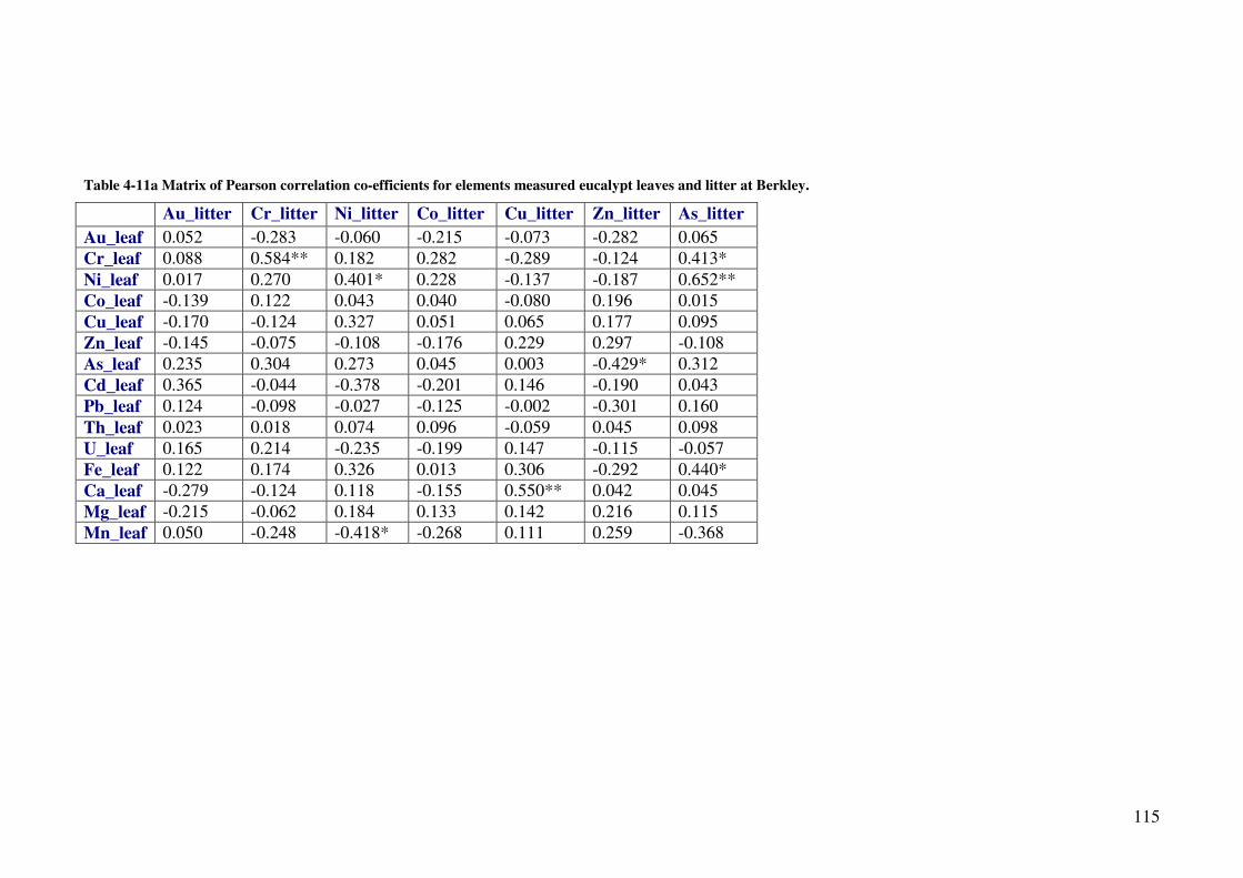
115

Table 4-11a Matrix of Pearson correlation co-efficients for elements measured eucalypt leaves and litter at Berkley.

Au_litter Cr_litter Ni_litter Co_litter Cu_litter Zn_litter As_litter

Au_leaf 0.052 -0.283 -0.060 -0.215 -0.073 -0.282 0.065

Cr_leaf 0.088 0.584** 0.182 0.282 -0.289 -0.124 0.413*

Ni_leaf 0.017 0.270 0.401* 0.228 -0.137 -0.187 0.652**

Co_leaf -0.139 0.122 0.043 0.040 -0.080 0.196 0.015

Cu_leaf -0.170 -0.124 0.327 0.051 0.065 0.177 0.095

Zn_leaf -0.145 -0.075 -0.108 -0.176 0.229 0.297 -0.108

As_leaf 0.235 0.304 0.273 0.045 0.003 -0.429* 0.312

Cd_leaf 0.365 -0.044 -0.378 -0.201 0.146 -0.190 0.043

Pb_leaf 0.124 -0.098 -0.027 -0.125 -0.002 -0.301 0.160

Th_leaf 0.023 0.018 0.074 0.096 -0.059 0.045 0.098

U_leaf 0.165 0.214 -0.235 -0.199 0.147 -0.115 -0.057

Fe_leaf 0.122 0.174 0.326 0.013 0.306 -0.292 0.440*

Ca_leaf -0.279 -0.124 0.118 -0.155 0.550** 0.042 0.045

Mg_leaf -0.215 -0.062 0.184 0.133 0.142 0.216 0.115

Mn_leaf 0.050 -0.248 -0.418* -0.268 0.111 0.259 -0.368

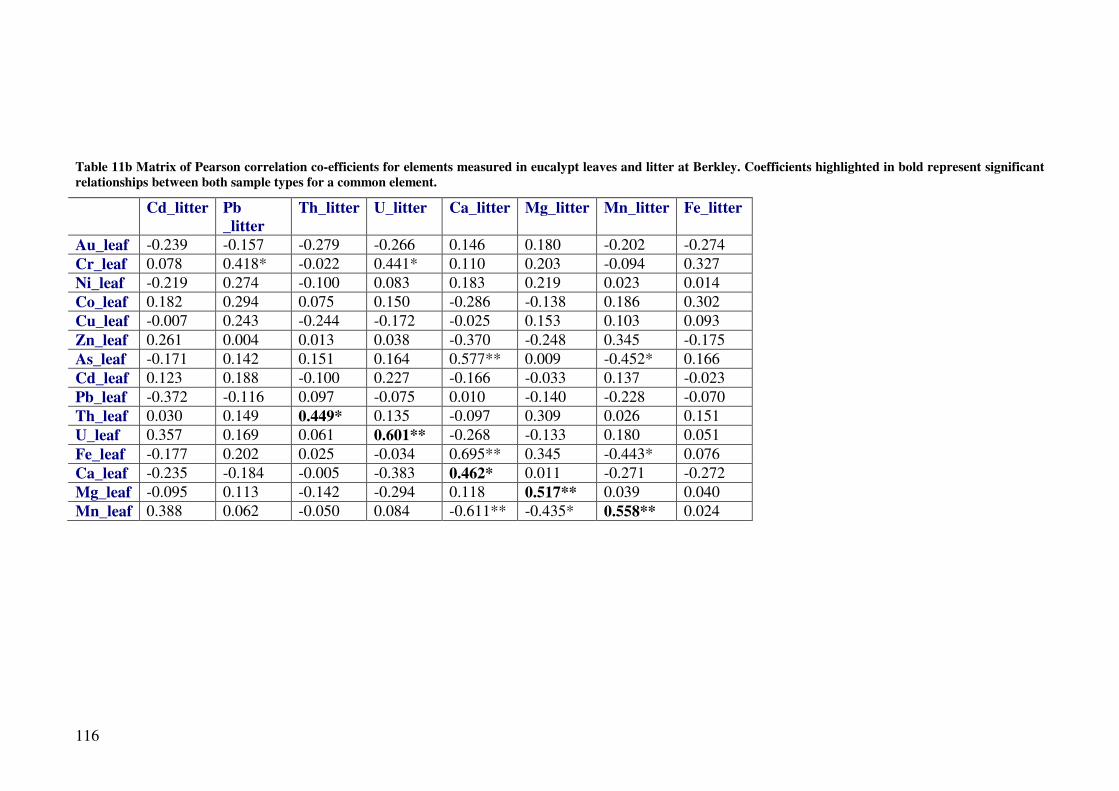
116

Table 11b Matrix of Pearson correlation co-efficients for elements measured in eucalypt leaves and litter at Berkley. Coefficients highlighted in bold represent significant

relationships between both sample types for a common element.

Cd_litter Pb

_litter

Th_litter U_litter Ca_litter Mg_litter Mn_litter Fe_litter

Au_leaf -0.239 -0.157 -0.279 -0.266 0.146 0.180 -0.202 -0.274

Cr_leaf 0.078 0.418* -0.022 0.441* 0.110 0.203 -0.094 0.327

Ni_leaf -0.219 0.274 -0.100 0.083 0.183 0.219 0.023 0.014

Co_leaf 0.182 0.294 0.075 0.150 -0.286 -0.138 0.186 0.302

Cu_leaf -0.007 0.243 -0.244 -0.172 -0.025 0.153 0.103 0.093

Zn_leaf 0.261 0.004 0.013 0.038 -0.370 -0.248 0.345 -0.175

As_leaf -0.171 0.142 0.151 0.164 0.577** 0.009 -0.452* 0.166

Cd_leaf 0.123 0.188 -0.100 0.227 -0.166 -0.033 0.137 -0.023

Pb_leaf -0.372 -0.116 0.097 -0.075 0.010 -0.140 -0.228 -0.070

Th_leaf 0.030 0.149 0.449* 0.135 -0.097 0.309 0.026 0.151

U_leaf 0.357 0.169 0.061 0.601** -0.268 -0.133 0.180 0.051

Fe_leaf -0.177 0.202 0.025 -0.034 0.695** 0.345 -0.443* 0.076

Ca_leaf -0.235 -0.184 -0.005 -0.383 0.462* 0.011 -0.271 -0.272

Mg_leaf -0.095 0.113 -0.142 -0.294 0.118 0.517** 0.039 0.040

Mn_leaf 0.388 0.062 -0.050 0.084 -0.611** -0.435* 0.558** 0.024

117

4.3. Discussion

4.3.1. Soil and plant response to buried mineralisation

The soils at Berkley showed a stronger response to the Au mineralisation than the plant

samples. However, both sample media showed good correspondence to the underlying

mineralisation despite the presence of a transported overburden. The association

between the plants and soils with the buried mineralisation does not, however, prove

any causative relationship between mineralisation, plant uptake and soil accumulation.

As both the plants and soils showed high responses to the regolith Au, it is inconclusive

whether deep biotic uplift as a mechanism of soil anomaly formation caused the high

concentrations of Au in the soil. Lintern et al. (1997) concluded that the vegetation

tended to reflect the concentrations in soil instead of the mineralisation, and that the

vegetation was cycling the ore elements in the surface only. At this site, the strongest

evidence that the vegetation seems to have taken up Au from depth comes from data

that show accumulation of Au in soil developed from a transported overburden that drill

cores show to be effectively barren of Au. The Au distribution with soil depth shows an

anomalous concentration of Au to a soil depth of 25 cm over mineralisation, after which

there is a sharp decline in Au concentration to 35 cm (Refer to Figure 4-13, soil depth

data for 320 00E soil pit). The plant samples (both leaf and litter) from this same

location showed responses of approximately 3-6 times background Au concentrations

(refer to Figure 4-16 and Figure 4-21). However, there are insufficient data for samples

greater than 35 cm depth and replication within the soils sampled at each depth interval

to support a hypothesis that the plants are taking up metals from depth.

Plants will recycle the Au in the surface but there is still the question of how the Au

came to accumulate in the soils developed from a barren transported overburden. Plants

are established at the same time the transported overburden was deposited over the

residual mineralised-profile (Rose et al. 1979). It is well known that plants are able to

root to significant depths (40-53 m; see Table 2-3,Chapter 2) (Canadell et al. 1996) in

search of nutrients and water. Even over relatively short geological time periods (ca.106

y), it is plausible that plants may be able to take up target ore and associated path finder

elements from depth, and deposit these into the surface soils at a much faster rate than

would normally be possible by physical mechanisms such as diffusion. Other

mechanisms of vertical ionic transport, such as capillary rise or evaporation (Keeling

2004; Mann et al. 2005), may be operating in unison in the semi-arid environment. Our

118

study site at Berkley showed accumulation of the target element Au in plants but also in

the soils, despite the barren transported overburden the plants and soils are overlying.

Thus, it is likely that plants at Berkley may have provided a vertical pathway of

migration for Au to accumulate in the surface soils, completely bypassing the

underlying transported overburden.

Our statistical analyses showed poor correlation between the concentrations of Au in the

soil and plants at Berkley, although both responded to the mineralisation. Anand et al.

(2007) similarly found that only the plants (Acacia spp.) showed the signature of the

underlying bedrock mineralisation and not their 10-20 cm soil samples from their study

at the Jaguar deposit near Kalgoorlie in Western Australia. Various other studies have

also shown a lack of correlation between the concentration of ore elements in soils and

plants (Lintern et al. 1997; Cohen et al. 1998; Cohen et al. 1999). The lack of

correlation between the soils and plants at our site and in the literature may be explained

by considering the different time frames applying to soil and plant accumulation. Soils

will integrate the geochemical signature of the mineralisation over time but plants may

not. Hence, the geochemical signature of the mineralisation that develops in the plants

could be a much more transient signal than that in the soils. Anand et al. (2007)

surmised that the lack of development of a soil anomaly was due to the low net primary

productivity of the vegetation and the low decomposition rates of the litter. Similarly,

litter removal by wind or water erosion before significant amounts of litter can

accumulate would also lead to low plant returns to the soil (Cohen et al. 1999). On the

other hand, a study in the Cobar area of NSW, Australia by Cohen et al. (1998)

concluded that an anomaly did not develop in the soils because the rate of leaching loss

from the soils was faster than the rate of accumulation of elements in the soil by plant

return. These observations support the conclusions of a mass balance exercise presented

earlier in this thesis, which showed that net accumulation of trace elements in soils

occurs via upward flux from plant uptake depending on the balance between ecosystem

net primary productivity and losses through soil erosion and leaching (Refer to Chapter

2: Literature Review; also refer to Chapter 5).

This balance between net accumulative and loss fluxes may perhaps explain why we

found the 10-25 cm soil enriched in Au. The loss fluxes of trace elements from the soils

at Berkley through erosion and leaching are minimal, since the landscape is relatively

flat and stable and the environment is semi-arid. Thus, the conditions for net trace

119

element accumulation in the soil are optimal at Berkley and accordingly, elevated

concentrations of Au and other trace elements were measured in the soils.

4.3.2. Soil and plant response to underlying lithology

The correspondence between the plants and soils with underlying lithology may be an

indication that the plants are taking up elements from deep in the buried regolith (Figure

4-5 - Figure 4-25). Both the plant and soil samples display chemically distinct trace

element “signatures” and may reflect the underlying lithological unit as suggested by

the results of the correlation analysis on the elements in each sample medium (Table

4-2-Table 4-5). For example, there is clear enrichment of Li, As, Ni, Zn in the soils

above the ultramafics in the west on the southern transect. There is also enrichment of

As, Pb, Cd, Co, Cr and Ni in both leaf and litter samples close to the

ultramafic/metabasalt contact at 318 970E. Large response ratios for Cd, Pb, Th and U

were detected in all samples over the pyroxenite unit. On closer examination, the

response ratios for these elements are closely clustered around 319 850E. Drill cores

across the pyroxenite unit indicate the presence of felsic intrusions and the high

concentrations of Pb, Th and U in the plants and soils may indicate the occurrence of a

felsic intrusion along the sampling transect. Large REE anomalies at this same location,

319 850E, on the southern transect in MMI soil samples further suggest the presence of

a felsic intrusion. There is also a strong anomaly contrast from the raw concentrations of

Th and U in plant samples (particularly litter samples) over the pyroxenite, with the

litter samples often surpassing the 10-25 cm soil samples in concentration for both

elements. The different sample media were useful in demarcating the underlying

lithology. It is interesting that the samples showed high responses over the lithological

contacts between the ultramafic and metabasalt (at 318 970E) and the metabasalt and

pyroxenite (at 319 970E) units. For example, there are clear peaks in the Pb, Zn, REE

and Au concentrations of the MMI and aqua regia soil samples above these two

contacts. Similar peaks were detected for Pb, Cr, As, Au, Cu, Zn and REE (U and Th) in

the litter and leaf samples near these same two lithological contacts. It is unclear why

the response ratios were significantly higher for some elements near these two

lithological contacts (ultramafic and metabasalt contact and the metabasalt and

pyroxenite contact further east). Contacts commonly experience increased weathering

activity due to chemical gradients that occur between the adjacent lithological rock units

(Isik Ece and Schroeder 2007). These elements may be more bioavailable or mobile at

the lithological boundaries that may be the result of the poorly exposed thrust fault in

120

the pyroxenite unit or the felsic intrusions. Cameron and Leybourne (2005) have

documented the movement of groundwater through permeable zones along fault lines

that once conducted hydrothermal fluids. The fault lines girdling the pyroxenite unit

may perhaps provide zones of permeability along which water may move more freely

than through the surrounding rocks. Further investigation with partial extractions of soil

samples, for example that targeting the organic pool in soils (extraction with sodium

pyrophosphate; see Chapter 3 (Hall et al. 1996)) may help clarify the presence of these

anomalies over the lithological contacts.

Litter samples gave better anomaly contrast to the underlying Au mineralisation than

the living plant tissue itself. Similarly, other workers have found better anomaly

contrast in litter and the humus soil horizon for Au and base mineral exploration

(Lintern et al. 1997). Anand et al. (2007) have suggested that the litter layer and the 0-4

cm soil horizon gave better anomaly contrasts than the mineral horizon (10-20 cm)

because the metals absorbed by living vegetation eventually accumulate in the litter

layer which is subsequently released into the 0-4 cm soil horizon. However, they

suggested that, because the 0-4 cm soil horizon was continually redistributed in the

landscape, little of the metals held in the 0-4 cm soil horizon get incorporated directly

into the underlying soil horizons. The same argument would apply even more so to the

litter layer. Further, the break-down of the litter layer and eventual leaching of metals

from the 0-4 cm to the deeper soil horizons may also be limited by the aridity of the

environment within which Berkley is sited. Bioturbation by ants and other soil fauna

could also redistribute the litter layer around the landscape. Within the Berkley soil

samples, we found that there were significant differences (student’s t-test,

α= 0.05) between the 0-4 cm and the 10-25 cm soil samples as reported in Anand et al.

(2007). However, the differences between the sampling depths differed with the type of

analysis (MMI or aqua regia) and only for certain elements. Both types of analysis

showed that only the Cu and Zn concentrations in the two soil depths differed

significantly. For Au, only the MMI samples showed a difference between the two soil

depths. Subsequently, we found no advantage in using soil sampled from the 0-4 cm

depth, in terms of additional information, over the 10-25cm sampling depth.

121

4.3.3. Biogeochemical accumulation in plants and soils in the presence of a

transported overburden

There is good correlation between surface response on the southern transect and the

buried mineralisation (Figure 4-3). Au mineralisation is found in the saprolite at depths

of greater than 35m in the eastern end of both sampling transects (Figure 4-1). Both the

plants and soils showed elevated concentrations of Au directly above the mineralisation

at 319 850E, despite the presence of 15 m of barren transported cover. Interestingly,

both types of soil analysis showed high Au responses at the eastern end of the transect,

whereas Au mineralisation was not detected in this area from the drill cores.

In contrast to the southern transect, the soils from the transect 225 m to the north

showed little to no response to the underlying mineralisation (Figure 4-4). The

mineralisation found beneath this transect is weaker and may explain the lack of

response in the soils. Litter samples from the northern transect were the only media to

give a Au response ratio larger than 2, with a peak response of about 3 ppb or 5 times

the background concentration at 319 750E. However, the drill core data showed no

significant Au accumulation in either the regolith or the underlying bedrock at this

location. A similar peak in Au concentration was detected further east along this

transect at 319 875E in both the litter and leaf samples. However, there is anomalous Au

present in the saprolite nearby at 319 850E as shown in the drill section at 6563 300N

(Figure 4-4).

The depth of transported cover does not seem to affect the accumulation of elevated

concentrations of elements in plants and soils. In the southern transect, the greatest

response obtained for Au from all sample media along the southern transect was at

319 850E, which has a cover depth of 15 m (Figure 4-3). There were low responses in

the sample media to the west of this location, where there is thickening cover (20-30 m),

and low responses to the east where there is thinning cover (15-0 m). Additionally, the

plant response to the mineralisation in our study at Berkley shows that depth of

transported overburden has no effect on the soil and plant response, particularly in the

northern transect. Work by Lintern (2007) has also shown no correlation between

transported overburden thickness and accumulation in vegetation (Eucalyptus

incrassata and Eucalyptus socialis). The depth of transported overburden at Berkley on

the northern transect is fairly uniform, with an average depth of 10 m, but the only

significant response was in the plant samples at two points along this transect (Figure

122

4-4). In addition, the land surface here is relatively flat (maximum difference in height

along this transect over a distance of 100 m was 4 m), hence, movement of material in

the north at present should be fairly limited. However, prior mass movement may have

flattened out the landscape. Further, the plant response was not always vertically over

mineralisation. Often, the plants that showed response to mineralisation were situated

approximately 25 m further west/east of the anomalous Au measured in the drill core.

Lintern et al. (1997) have suggested that the lack of correlation between soils and

vegetation may be because the soil horizon sampled may not be the same as that from

which the vegetation takes up water and nutrients. By that same token, vegetation can

also be thought to sample a wide volume of regolith, which could conceivably dilute the

geochemical signature of the hidden mineralisation. Plant accumulation is also

dependent on whether the roots are within reach of mineralisation (see also later

discussion on the effect of biogeochemical processes on the development of plant and

vegetation anomalies). The accumulation of ore elements in plants at Berkley is

therefore dependent on rooting depth and may not necessarily correspond to surface soil

concentrations. The drill sections are also from transects parallel to, but not directly

beneath, our own sampling transects and hence the mineralisation found in the drill

lines may not line up exactly to our sampling transects.

Au anomalies were detected in several plant and soil samples beyond the existing RAB

drill lines. Over the ultramafics in the west of the southern transect, a Au anomaly in

litter was detected (Figure 4-18). These anomalous concentrations in the samples may

indicate the presence of more Au mineralisation at depth and may represent a further

extension of the mineralisation that was detected in the drill cores.

4.4. Conclusions

Plants and soils were not only useful in indicating the presence of Au mineralisation

underlying several metres of transported overburden but were also incorporating the

geochemical signature of each lithological unit despite the presence of the overburden.

Although the Au response ratios in the soil samples were greater than lithologically

related elements, the Au response ratios in the vegetation samples were lower than that

of the lithologically related elements. The strongest evidence that the vegetation seems

to have taken up Au from depth at Berkley comes from data that showed accumulation

of Au in soil developed from a transported overburden that drill cores show to be

123

effectively barren of Au. Further, the presence of soil anomalies from both MMI and

aqua regia analyses indicates that the optimal conditions for accumulation of trace

elements in the soils are present at Berkley because of minimal loss fluxes operating in

this particular environment.

125

CHAPTER FIVE

Field study on trace element biogeochemistry and the formation of soil

geochemical anomalies II: the development of soil and vegetation

anomalies in a calcrete-dominated landscape

Torquata Prospect, Eucla Basin, Western Australia

5. Introduction

The findings from the second case study on soil and vegetation anomalies are presented

in this chapter. The study site, Torquata, makes for an interesting study because minable

quantities of gold are predominately associated with near-surface (1-5 m deep)

pedogenic calcrete (referring both to the calcareous surface soils horizon and the

calcrete nodules developed within them) developed in a thick transported overburden. In

arid regions of Australia, pedogenic calcrete developed in residual soils, and soils

developed in transported material over bedrock mineralisation, is commonly associated

with anomalous Au (Lintern et al. 2006). The anomalous Au in the calcrete at Torquata

is therefore not technically “mineralisation”, since there is no underlying bedrock

mineralisation. Although anomalous concentrations of gold as high as 3 ppm have been

found in the calcrete, extensive drilling in the area has shown no gold mineralisation

beneath 30-100 m of transported material.

The formation of calcrete has been widely studied because of its importance as a sample

medium for Au exploration (Anand et al. 1997; Lintern 2001; Lintern et al. 2006;

Mumm et al. 2007). Pedogenic calcrete is commonly found in areas with an average

annual rainfall between 100-600 mm and forms in the vadose zone (unsaturated soil

horizon) (Anand et al. 1997; Anand et al. 2002). Some evidence suggests that plants,

mycorrhizal fungi and microorganisms are extensively involved in the formation of

pedogenic calcrete (Verboom et al. 2006; Singh et al. 2007). Carbon isotope data has

shown that the C in the carbonate originates from a mixture of C3 and C4

palaeovegetation (Lintern et al. 2006), provided no subsequent fractionation occurs in

the process. Lintern et al. (2006) suggested that the Au then eventually comes to be

associated with the calcrete through plant uptake from depth and eventual deposition in

the surface soil where both the Au and calcium carbonate precipitate out from solution

(the carbonate resulting from a combination of plant C and CO2 from soil respiration).

Due to the constant processes of dissolution and precipitation that Ca and Au undergo in

126

the soil profile (the vadose zone) with the changing seasons, there is usually a strong

linear relationship between the two. The relative mobility of Ca and Au in these

environments (calcareous soil and in the vadose zone) implies that we might also expect

a relationship between Ca and Au within the plant material. The model by Lintern et al.

(2006) is however based on the mobilisation of Au from a bedrock source. The situation

at Torquata, in contrast, is one where there is no underlying bedrock Au mineralisation.

This begs the question of where the Au in the Torquata near surface calcrete originates

from. Drilling in the area shows the presence of a redox boundary at depth (between 50-

100 m deep) and also the presence of a deep water table (highest level at 46 m). Three

possible scenarios can be drawn up to explain the lack of bedrock Au:

Scenario (1) Torquata is situated on the edge of the Eucla Basin and could possibly

have served as a drainage point for several palaeostreams carrying

minute quantities of Au originating from the Yilgarn Plateau. In this

scenario, there is no point source of Au as such;

Scenario (2) Groundwater levels in the geologic past may have been higher and if

only a small bedrock mineralisation was present, the waters may have

long leached the Au out to sea. The Au locked up in the calcrete could be

the remnant signature of past Au mineralisation;

Scenario (3) The mineralisation that may be the source of the anomalous Au in

calcrete may simply be located beyond the extent of current drill lines.

In all three scenarios, the biogeochemical process of translocating and accumulating the

Au in the calcrete as described by Lintern et al. (2006) would still be possible. A

biogeochemical study of the prospect was carried out to determine whether vegetation

and soil sampling could generate a biogeochemical signature that may in turn provide

some clues as to the whereabouts of the source of the Au in the calcrete. Thus the aims

of the biogeochemical study at Torquata were: i) To determine if deep biotic uplift of

Au has led to the accumulation of trace elements in the near surface calcrete horizon

developed within the transported overburden; ii) To determine the source of the calcrete

Au and; iii) To generate input data for numerical modelling.

127


5.1.1. Site description

Torquata is located 210 km south east of Kambalda in Western Australia (Figure 5-1).

The tenement is situated at the edge of the sedimentary Eucla Basin abutting the Yilgarn

Plateau. The Eucla Basin is known for its heavy mineral and Au placer deposits

(Government of South Australia 2007). The climate at Torquata is semi-arid with an

average annual rainfall of approximately 250 mm, which falls mainly in the winter

months between June and August. The landscape around Torquata is relatively flat and

erosional loss from the soil should be minimal. Vegetation on the site was recently

burned in a wildfire (3 months prior to the sampling exercise); however, a few stands of

eucalypts (Eucalyptus cylindrocarpa) were left intact on the northern sampling transect,

6511 200N (see Plates 5-1 and 5-2). Young vegetation regrowth had already been

established at the base of burned trees (see Plate 5-1). The gold at Torquata is mainly

present in the calcrete horizon in the near surface at an average depth of 5 m. The

weathered regolith at Torquata is covered by a transported overburden of variable

thickness which is of marine origin (predominantly shales). The transported cover

generally increases in thickness to the east of the site to depths greater than 100 m. Soil

pits dug at the site showed that the top of the calcareous soil horizon starts at about 10-

25 cm. A layer of calcrete nodules (ranging in size from 2 mm to 50 mm) is present at

about 25–35 cm depth (The layer of calcrete nodules may extend lower than the depth

of the soil pits). The in situ regolith comprises of mudstones or shales of variable

thickness between 30-60 m. The mudstone/shale regolith is underlain by a weathered

uniform sedimentary rock of Proterozoic age. Initial RAB drilling of the area was

carried out at the site prior to the start of this current biogeochemical study, indicated

the presence of a variable redox boundary at between 20 m to greater than 60 m depth.

There are no obvious active drainage channels at the surface and drilling has not

discovered any palaeodrainage channels. There is a variable water table present in the

regolith with the highest water level recorded in the drill bores at approximately 40 m

depth.

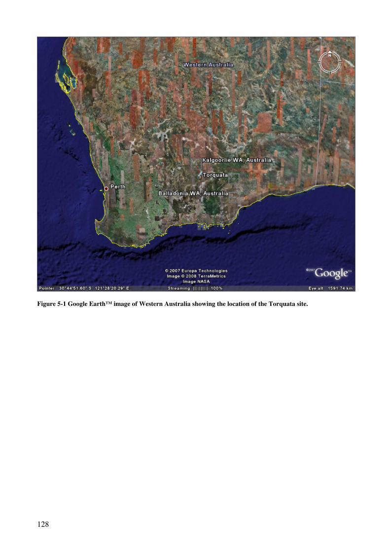
128

Figure 5-1 Google Earth™ image of Western Australia showing the location of the Torquata site.

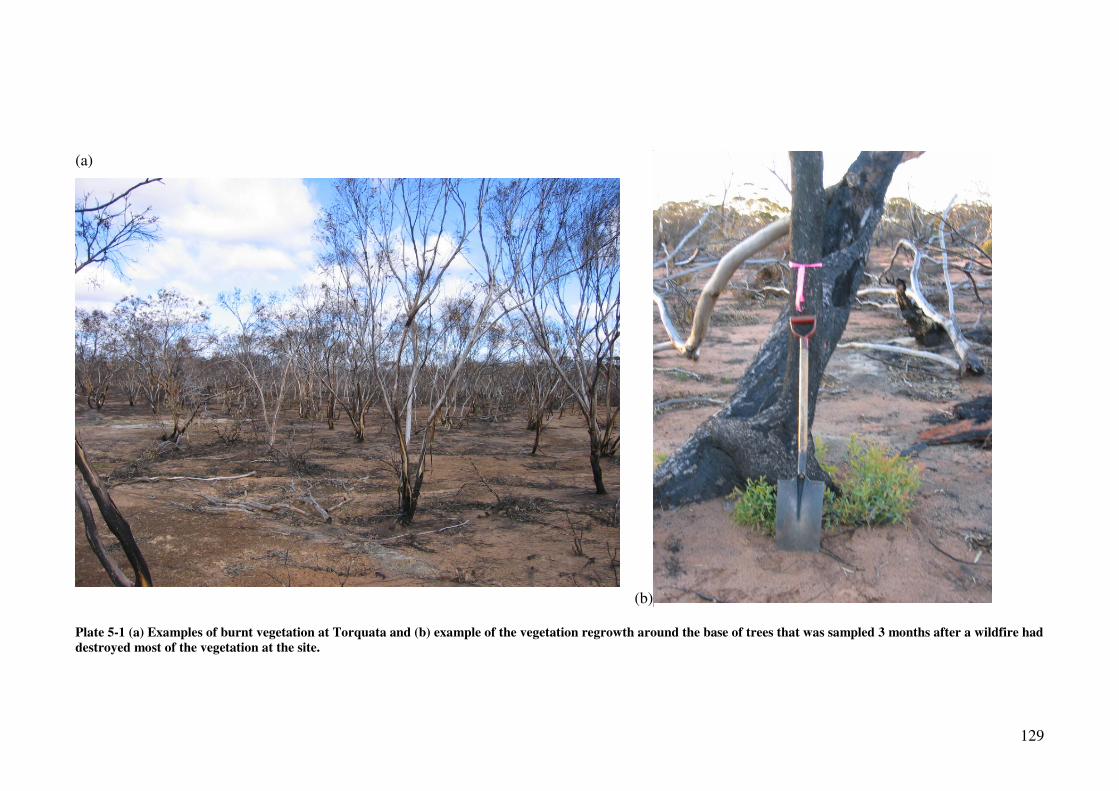
129

(a)

(b)

Plate 5-1 (a) Examples of burnt vegetation at Torquata and (b) example of the vegetation regrowth around the base of trees that was sampled 3 months after a wildfire had

destroyed most of the vegetation at the site.

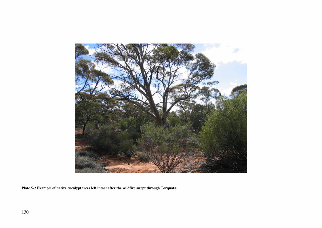
130

Plate 5-2 Example of native eucalypt trees left intact after the wildfire swept through Torquata.

131

5.1.2. Sampling Design

The same sampling design and sample processing procedures were applied to the

Torquata site as was applied at Berkley. The reader is referred to Chapter 4 for more

information regarding the sampling methods. The sampling at the Torquata prospect

was carried out along two parallel transects, 6510 440 N and 6511 200 N (GPS

database: UTM ’84), between 24 — 25 October 2005. Sampling transects were between

previous drilling lines to minimise possible contamination of surface soils and

vegetation with drill dust. Similarly to Berkley, of the unburnt trees, no sign of plant

stress was observed at Torquata. Due to the recent fire at Torquata, where vegetation

was burned, the vegetation regrowth (the re-sprouting eucalypt plants at the base of a

burned tree) was sampled instead (see Plate 5-1 for an example of regrowth found at the

site). Leaves and fruits, as well as pictures of the unburnt trees were sent to the WA

Herbarium for identification (Western Australian Herbarium, George Street,

Kensington, Western Australia (6151)). Additionally, the coarse fraction (>2 mm) of the

soils collected from the 35 cm deep soil pits were sent for analysis by ICP/MS for Au,

As, Ca, Co, Cu, Fe, Mn, Mg, Pb and Zn to Ultratrace (Ultra Trace Pty Ltd, 58

Sorbonne Crescent, Canning Vale, Western Australia 6155).

5.1.3. Statistics

All data were initially log transformed prior to any statistical testing to normalise the

positive skewness in the data. Response ratios were then calculated for each element

using the 25th

percentile method described by Karajas (1999), where the 25th

percentile

value for pooled data from both transects has been taken to be the background value for

any element. Z scores were calculated for individual elements measured in both soil and

vegetation samples as a definitive measure of identifying anomalous concentrations,

using the formula: σ

xx −

(where x is the normalised measured concentration in the

sample medium, x is the mean of concentrations measured in the samples and σ is the

standard deviation of the population measured). x was calculated by averaging the

concentrations across both transects. A Z score of 1.6 was used as a threshold to

demarcate any samples within the highest 5% of the measured concentrations in the soil

samples. Negative anomalies are not discussed for the field results because they are not

as useful in demarcating buried ores (Rose et al. 1979). Regression analyses were also

132

applied on the data using ANOVA in Microsoft Excel®. Significance testing on

correlation data was carried out in SAS statistical software package (SAS Institute Inc.

2006). Comparisons of data between sample media were also carried out using paired

two-sample student’s t-test in Microsoft Excel®.

5.2. Results

5.2.1. Au in near surface calcrete

The highest concentration of Au at Torquata is associated with the pedogenic calcrete

horizon in the near surface (<5 m) of the transported overburden. Concentrations greater

than 100 ppb of Au have been measured in the surficial calcrete horizon; both in the

nodular calcrete and the calcareous soil horizon (Figure 2 and 3). Concentrations of Au

between 50 and 100 ppb have also been measured deeper in the overburden and in the in

situ mudstone/shales. Figure 5-2 (b) and Figure 5-3 (b) show the drill core cross

sections taken from transects close to the sampling transects. Drill data 140 m south of

our southern sampling transect (6510 440N) show concentrations of 30 – 74 ppb in the

top 5 m of calcrete horizon between 574 200E and 574 300E. High Au concentrations

of 21-700 ppb were measured deeper in the eastern most core of the 6510 440N drill

transect at 45-55 m depths. Similarly, drill data 60 m north of the 6510 440N sampling

transect also show high Au concentrations of 28-142 ppb within the top 5 m of the

transported overburden, in the calcrete horizon (Figure 2 (c)). Concentrations of Au

ranging from 26-230 ppb were found in the weathered in situ mudstone/shales between

50 and 60 m depth to the east of the drill transects. In the extended drilling line 100 m

south of the 6511 200N transect, 26-133 ppb of Au was measured in the top 5 m of the

transported overburden that extends east of 574 100E (Figure 5-3 (b) and (c)).

Concentrations of Au as high as 2.9 ppm were found in the transported overburden at

depths of between 20 m and 30 m. There is also some Au in the in situ material between

574 100E and 574 400E. Generally, where elevated concentrations of Au occur in the

surface 5 m of a drill core, there are similarly elevated concentrations of Au within that

same drill core, about 20-30 m deeper. Au data from all three drill sections, particularly

the drill sections at 6510 500N and 6511 100N, show that anomalous concentrations of

Au occur irregularly at different depths down the drill profile.

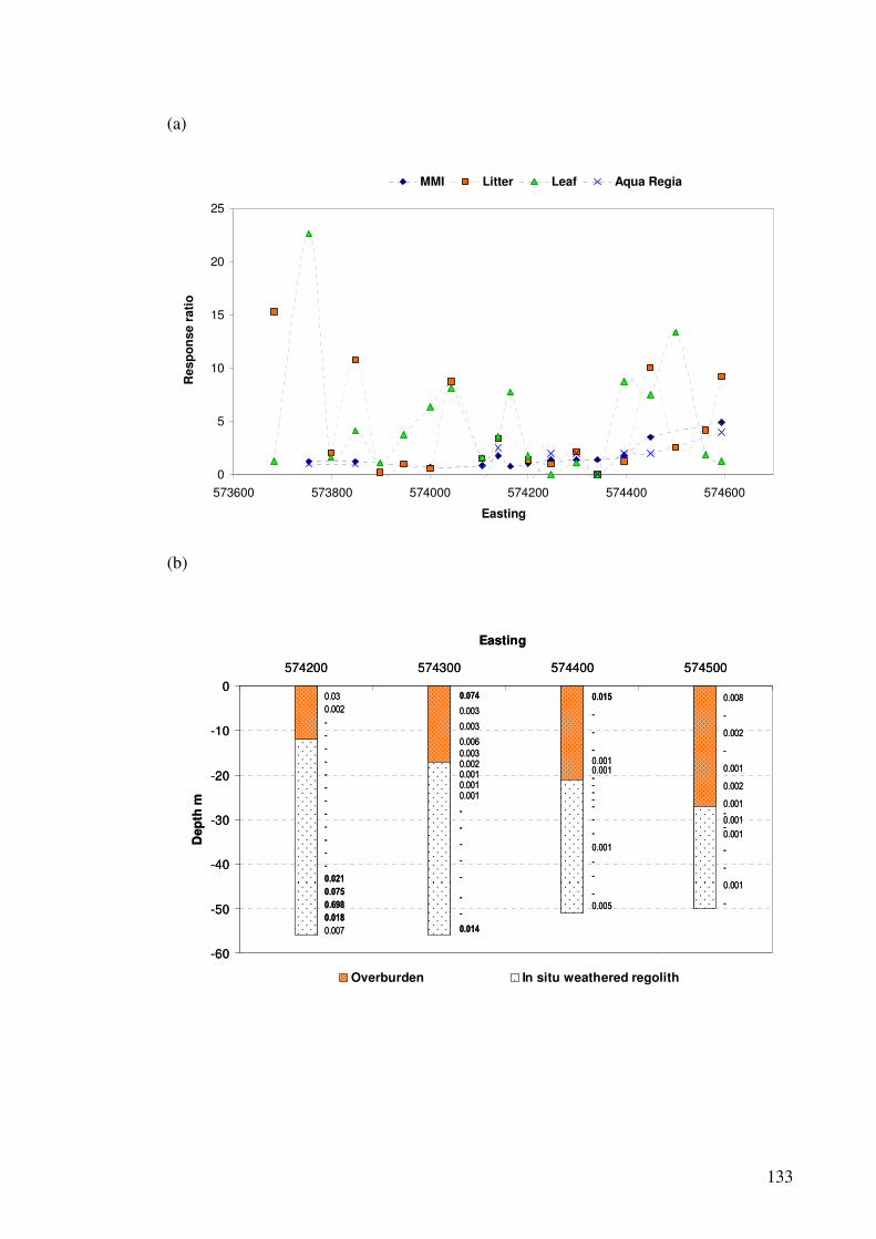
133

(a)

0

5

10

15

20

25

573600 573800 574000 574200 574400 574600

Easting

Re

sp

on

se

ra

tio

MMI Litter Leaf Aqua Regia

(b)

-60

-50

-40

-30

-20

-10

0

574200 574300 574400 574500

Easting

De

pth

m

Overburden In situ weathered regolith

0.03

0.002

-

-

-

-

-

-

-

-

-

-

-

-

0.021

0.075

0.698

0.018

0.007

0.074

0.003

0.003

0.006

0.003

0.002

0.001

0.001

0.001

-

-

-

-

-

-

-

0.014

0.015

-

-

-

0.001

0.001-----

-

-

0.001

-

-

-

0.005

0.008

-

0.002

-

0.001

0.002

0.001

-0.001-0.001

-

-

0.001

-

-60

-50

-40

-30

-20

-10

0

574200 574300 574400 574500

Easting

De

pth

m


0.03

0.002

-

-

-

-

-

-

-

-

-

-

-

-

0.021

0.075

0.698

0.018

0.007

0.074

0.003

0.003

0.006

0.003

0.002

0.001

0.001

0.001

-

-

-

-

-

-

-

0.014

0.015

-

-

-

0.001

0.001-----

-

-

0.001

-

-

-

0.005

0.008

-

0.002

-

0.001

0.002

0.001

-0.001-0.001

-

-

0.001

-

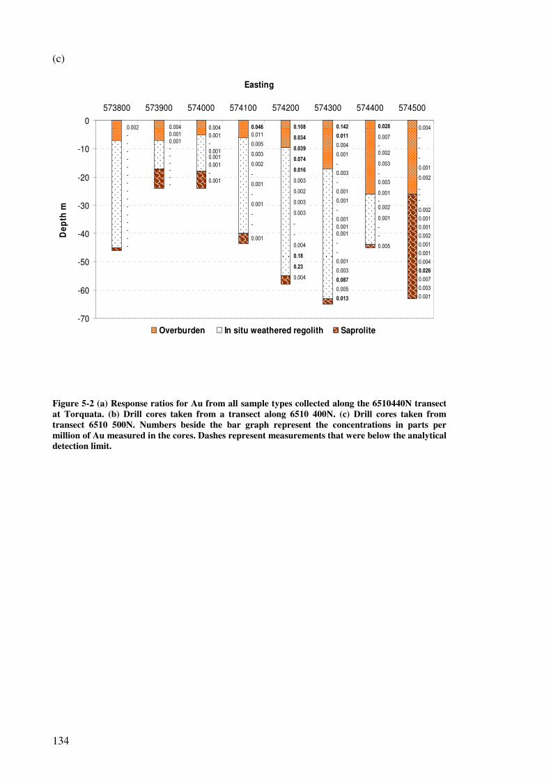
134

(c)

-70

-60

-50

-40

-30

-20

-10

0

573800 573900 574000 574100 574200 574300 574400 574500

Easting

De

pth

m

Overburden In situ weathered regolith Saprolite

0.002

-

-

-

-

-

-

-

-

-

-

-

-

-

-

-

0.004

0.001

0.001

-

-

-

-

-

-

0.004

0.001

-

0.001

0.001

0.001

-

0.001

0.046

0.011

0.005

0.003

0.002

-

0.001

-

0.001

-

-

0.001

0.108

0.034

0.039

0.074

0.016

0.003

0.002

0.003

0.003

-

-

0.004

0.18

0.23

0.004

0.142

0.011

0.004

0.001

-

0.003

-

0.001

0.001

-

0.001

0.001

0.001

-

-

0.001

0.003

0.087

0.005

0.013

0.028

0.007

-

0.002

0.003

-

0.003

0.001

-

0.002

0.001

-

-

0.005

0.004

-

-

-

0.001

0.002

-

-

-

0.002

0.001

0.001

0.002

0.001

0.001

0.004

0.026

0.007

0.003

0.001

Figure 5-2 (a) Response ratios for Au from all sample types collected along the 6510440N transect

at Torquata. (b) Drill cores taken from a transect along 6510 400N. (c) Drill cores taken from

transect 6510 500N. Numbers beside the bar graph represent the concentrations in parts per

million of Au measured in the cores. Dashes represent measurements that were below the analytical

detection limit.

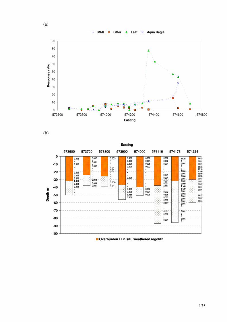
135

(a)

0

10

20

30

40

50

60

70

80

90

573600 573800 574000 574200 574400 574600 574800

Easting

Re

sp

on

se r

ati

o

MMI Litter Leaf Aqua Regia

(b)

-100

-90

-80

-70

-60

-50

-40

-30

-20

-10

0

573600 573700 573800 573900 574000 574116 574176 574224

Easting

De

pth

m


0.004

-

0.002

-

-

0.001

0.002

0.003

0.011

0.004

0.004

-

-

-

0.007-0.001-0.002------0.010

0.003

0.001

0.003-----0.0010.001-----0.008-0.001

0.003

0.002

0.001

0.001

-

-

-

0.001

-

-

-

0.001

0.003

0.011

0.001

0.009

0.001

0.005

0.002

-

-

-

-

-

-

-

0.002

0.004

0.005

0.008

0.002

0.001

-

-

-

0.001

0.001

0.001

0.001

0.001

-

0.002

0.030

0.002

0.002

0.001

-

-

0.001

0.002

-

0.001

-

0.026

0

0.001

0

0

0.004

0.001

0.004

0.001

0.002

0.009

0.140

0.129

0.001

0.002

0.001

0.001

0.001

0.001

0

-

0.001

0

0

0.001

0

0.053

0.001

0.001

0.033

0.210

2.290

0.800

0.005

0.003

0.001

0.002

0.001

0.001

-

0.057

0.002

0.004

-100

-90

-80

-70

-60

-50

-40

-30

-20

-10

0

573600 573700 573800 573900 574000 574116 574176 574224

Easting

De

pth

m


0.004

-

0.002

-

-

0.001

0.002

0.003

0.011

0.004

0.004

-

-

-

0.007-0.001-0.002------0.010

0.003

0.001

0.003-----0.0010.001-----0.008-0.001

0.003

0.002

0.001

0.001

-

-

-

0.001

-

-

-

0.001

0.003

0.011

0.001

0.009

0.001

0.005

0.002

-

-

-

-

-

-

-

0.002

0.004

0.005

0.008

0.002

0.001

-

-

-

0.001

0.001

0.001

0.001

0.001

-

0.002

0.030

0.002

0.002

0.001

-

-

0.001

0.002

-

0.001

-

0.026

0

0.001

0

0

0.004

0.001

0.004

0.001

0.002

0.009

0.140

0.129

0.001

0.002

0.001

0.001

0.001

0.001

0

-

0.001

0

0

0.001

0

0.053

0.001

0.001

0.033

0.210

2.290

0.800

0.005

0.003

0.001

0.002

0.001

0.001

-

0.057

0.002

0.004

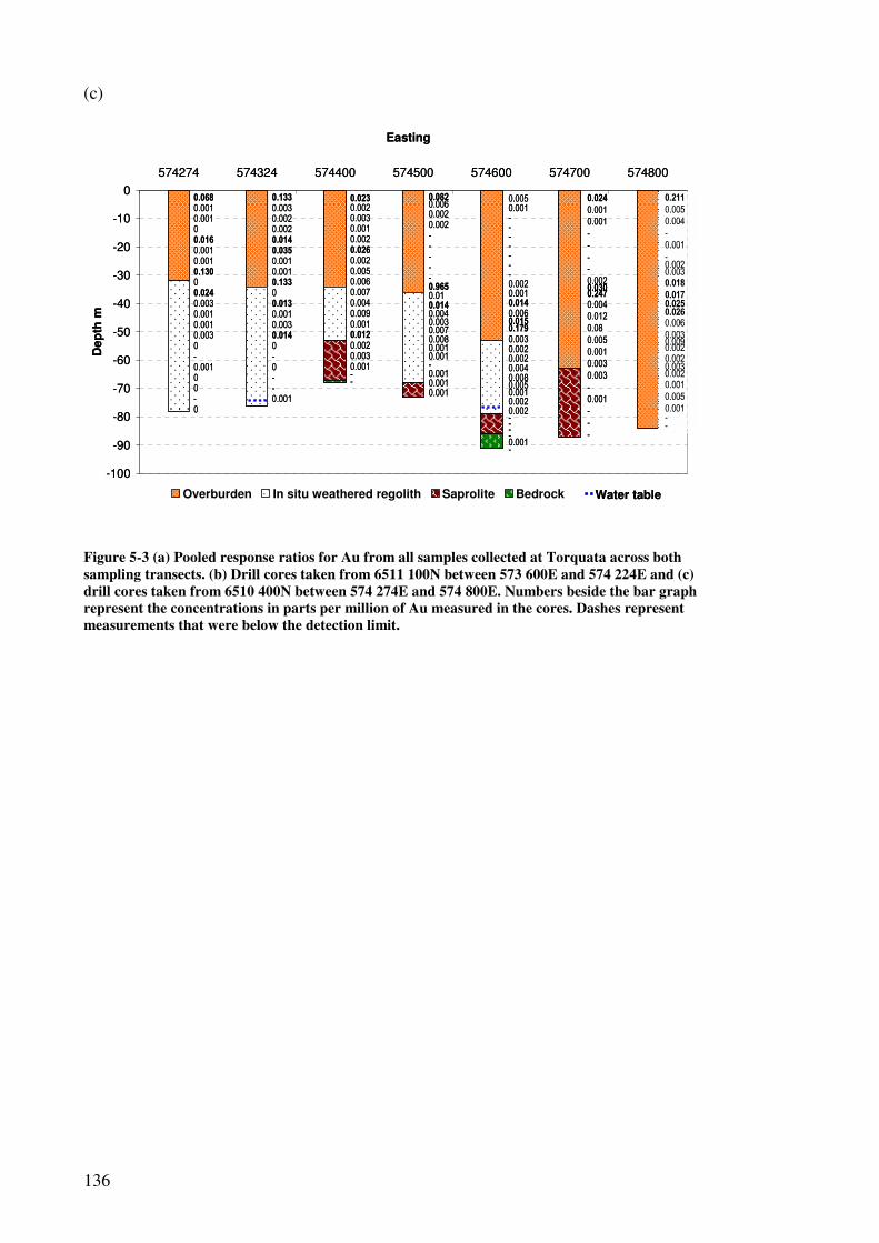
136

(c)

-100

-90

-80

-70

-60

-50

-40

-30

-20

-10

0

574274 574324 574400 574500 574600 574700 574800

Easting

Dep

th m

Overburden In situ weathered regolith Saprolite Bedrock Water table

0.068

0.001

0.001

0

0.016

0.001

0.001

0.130

0

0.024

0.003

0.001

0.001

0.003

0

-

0.001

0

0

-

0

0.133

0.003

0.002

0.002

0.014

0.035

0.001

0.001

0.133

0

0.013

0.001

0.003

0.014

0

-

0

-

-

0.001

0.023

0.002

0.003

0.001

0.002

0.026

0.002

0.005

0.006

0.007

0.004

0.009

0.001

0.012

0.002

0.003

0.001--

0.0820.006

0.002

0.002

-

-

-

-

-0.965

0.01

0.0140.0040.0030.007

0.0080.0010.001-

0.001

0.001

0.001

0.005

0.001

-

-

-

-

-

-

-

0.002

0.001

0.014

0.0060.0150.179

0.003

0.002

0.002

0.004

0.0080.0050.001

0.002

0.002----0.001-

0.024

0.001

0.001

-

-

-

-

0.0020.0300.247

0.004

0.012

0.08

0.005

0.001

0.003

0.003

-

0.001

-

-

-

0.211

0.005

0.004

-

0.001

-0.0020.003

0.018

0.0170.0250.026

0.006

0.0030.0090.002

0.0020.0030.002

0.001

0.005

0.001--

-100

-90

-80

-70

-60

-50

-40

-30

-20

-10

0

574274 574324 574400 574500 574600 574700 574800

Easting

Dep

th m

Overburden In situ weathered regolith Saprolite Bedrock Water table

0.068

0.001

0.001

0

0.016

0.001

0.001

0.130

0

0.024

0.003

0.001

0.001

0.003

0

-

0.001

0

0

-

0

0.133

0.003

0.002

0.002

0.014

0.035

0.001

0.001

0.133

0

0.013

0.001

0.003

0.014

0

-

0

-

-

0.001

0.023

0.002

0.003

0.001

0.002

0.026

0.002

0.005

0.006

0.007

0.004

0.009

0.001

0.012

0.002

0.003

0.001--

0.0820.006

0.002

0.002

-

-

-

-

-0.965

0.01

0.0140.0040.0030.007

0.0080.0010.001-

0.001

0.001

0.001

0.005

0.001

-

-

-

-

-

-

-

0.002

0.001

0.014

0.0060.0150.179

0.003

0.002

0.002

0.004

0.0080.0050.001

0.002

0.002----0.001-

0.024

0.001

0.001

-

-

-

-

0.0020.0300.247

0.004

0.012

0.08

0.005

0.001

0.003

0.003

-

0.001

-

-

-

0.211

0.005

0.004

-

0.001

-0.0020.003

0.018

0.0170.0250.026

0.006

0.0030.0090.002

0.0020.0030.002

0.001

0.005

0.001--

Figure 5-3 (a) Pooled response ratios for Au from all samples collected at Torquata across both

sampling transects. (b) Drill cores taken from 6511 100N between 573 600E and 574 224E and (c)

drill cores taken from 6510 400N between 574 274E and 574 800E. Numbers beside the bar graph

represent the concentrations in parts per million of Au measured in the cores. Dashes represent

measurements that were below the detection limit.

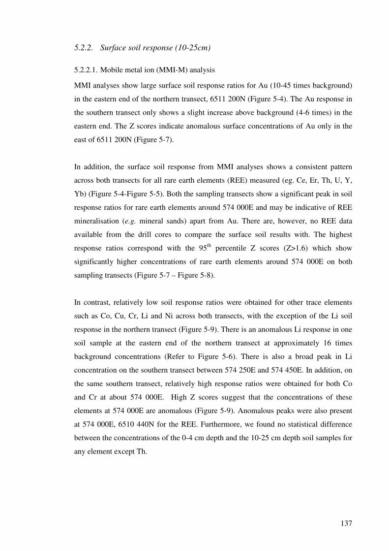
137

5.2.2. Surface soil response (10-25cm)

5.2.2.1. Mobile metal ion (MMI-M) analysis

MMI analyses show large surface soil response ratios for Au (10-45 times background)

in the eastern end of the northern transect, 6511 200N (Figure 5-4). The Au response in

the southern transect only shows a slight increase above background (4-6 times) in the

eastern end. The Z scores indicate anomalous surface concentrations of Au only in the

east of 6511 200N (Figure 5-7).

In addition, the surface soil response from MMI analyses shows a consistent pattern

across both transects for all rare earth elements (REE) measured (eg. Ce, Er, Th, U, Y,

Yb) (Figure 5-4-Figure 5-5). Both the sampling transects show a significant peak in soil

response ratios for rare earth elements around 574 000E and may be indicative of REE

mineralisation (e.g. mineral sands) apart from Au. There are, however, no REE data

available from the drill cores to compare the surface soil results with. The highest

response ratios correspond with the 95th

percentile Z scores (Z>1.6) which show

significantly higher concentrations of rare earth elements around 574 000E on both

sampling transects (Figure 5-7 – Figure 5-8).

In contrast, relatively low soil response ratios were obtained for other trace elements

such as Co, Cu, Cr, Li and Ni across both transects, with the exception of the Li soil

response in the northern transect (Figure 5-9). There is an anomalous Li response in one

soil sample at the eastern end of the northern transect at approximately 16 times

background concentrations (Refer to Figure 5-6). There is also a broad peak in Li

concentration on the southern transect between 574 250E and 574 450E. In addition, on

the same southern transect, relatively high response ratios were obtained for both Co

and Cr at about 574 000E. High Z scores suggest that the concentrations of these

elements at 574 000E are anomalous (Figure 5-9). Anomalous peaks were also present

at 574 000E, 6510 440N for the REE. Furthermore, we found no statistical difference

between the concentrations of the 0-4 cm depth and the 10-25 cm depth soil samples for

any element except Th.

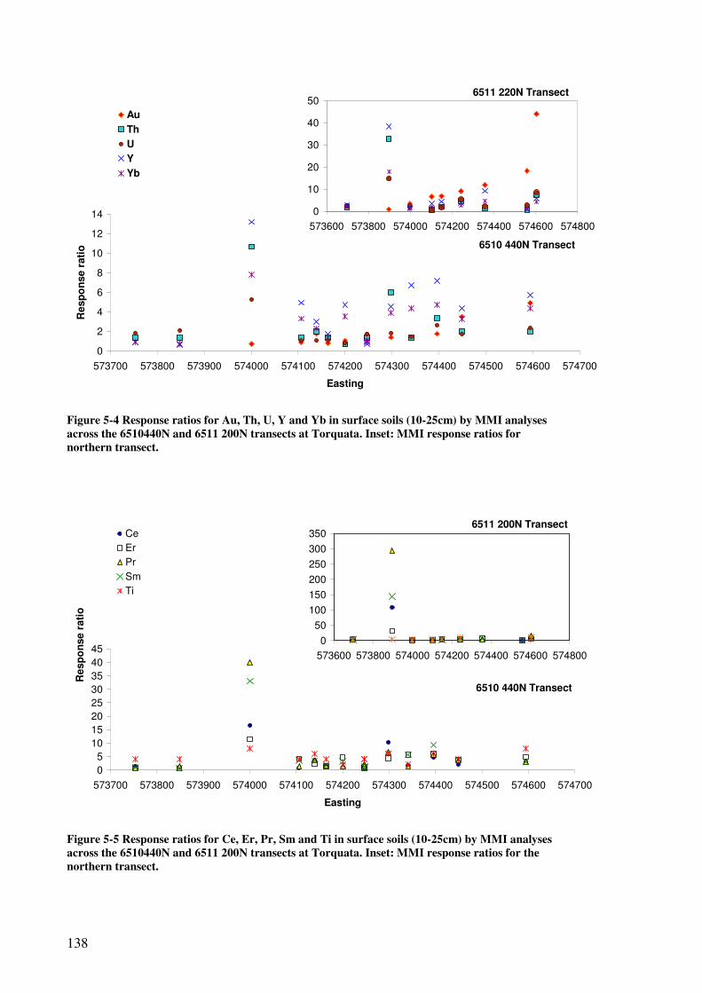
138

6510 440N Transect

0

2

4

6

8

10

12

14

573700 573800 573900 574000 574100 574200 574300 574400 574500 574600 574700

Easting

Re

sp

on

se

rati

o

Au

Th

U

Y

Yb

6511 220N Transect

0

10

20

30

40

50

573600 573800 574000 574200 574400 574600 574800

Figure 5-4 Response ratios for Au, Th, U, Y and Yb in surface soils (10-25cm) by MMI analyses

across the 6510440N and 6511 200N transects at Torquata. Inset: MMI response ratios for

northern transect.

6510 440N Transect

0

5

10

15

20

25

30

35

40

45

573700 573800 573900 574000 574100 574200 574300 574400 574500 574600 574700

Easting

Re

sp

on

se

rati

o

Ce

Er

Pr

Sm

Ti

6511 200N Transect

0

50

100

150

200

250

300

350

573600 573800 574000 574200 574400 574600 574800

Figure 5-5 Response ratios for Ce, Er, Pr, Sm and Ti in surface soils (10-25cm) by MMI analyses

across the 6510440N and 6511 200N transects at Torquata. Inset: MMI response ratios for the

northern transect.

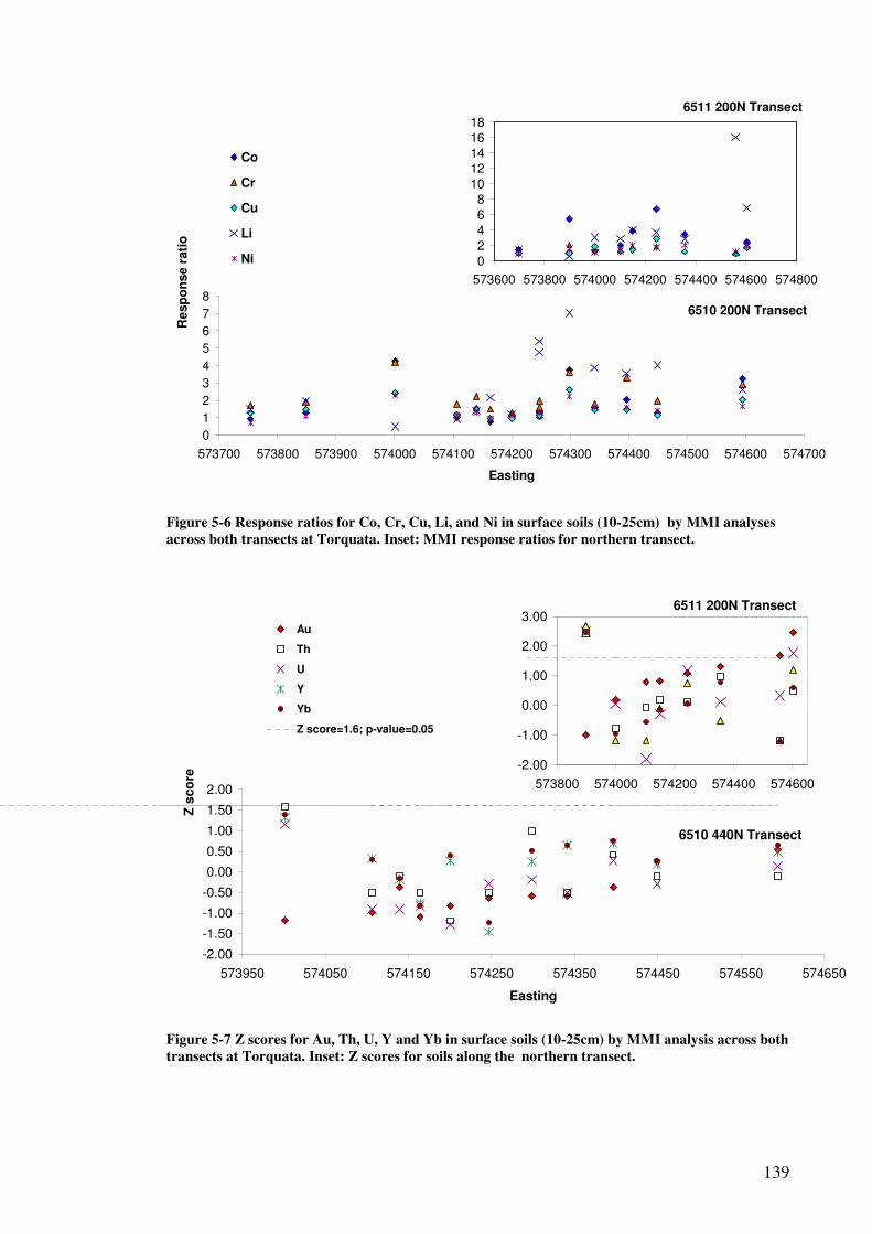
139

6510 200N Transect

0

1

2

3

4

5

6

7

8

573700 573800 573900 574000 574100 574200 574300 574400 574500 574600 574700

Easting

Re

sp

on

se

rati

o

Co

Cr

Cu

Li

Ni

6511 200N Transect

0

24

6

810

1214

1618

573600 573800 574000 574200 574400 574600 574800

Figure 5-6 Response ratios for Co, Cr, Cu, Li, and Ni in surface soils (10-25cm) by MMI analyses

across both transects at Torquata. Inset: MMI response ratios for northern transect.

6510 440N Transect

-2.00

-1.50

-1.00

-0.50

0.00

0.50

1.00

1.50

2.00

573950 574050 574150 574250 574350 574450 574550 574650

Easting

Z s

co

re

Au

Th

U

Y

Yb

Z score=1.6; p-value=0.05

6511 200N Transect

-2.00

-1.00

0.00

1.00

2.00

3.00

573800 574000 574200 574400 574600

Figure 5-7 Z scores for Au, Th, U, Y and Yb in surface soils (10-25cm) by MMI analysis across both

transects at Torquata. Inset: Z scores for soils along the northern transect.

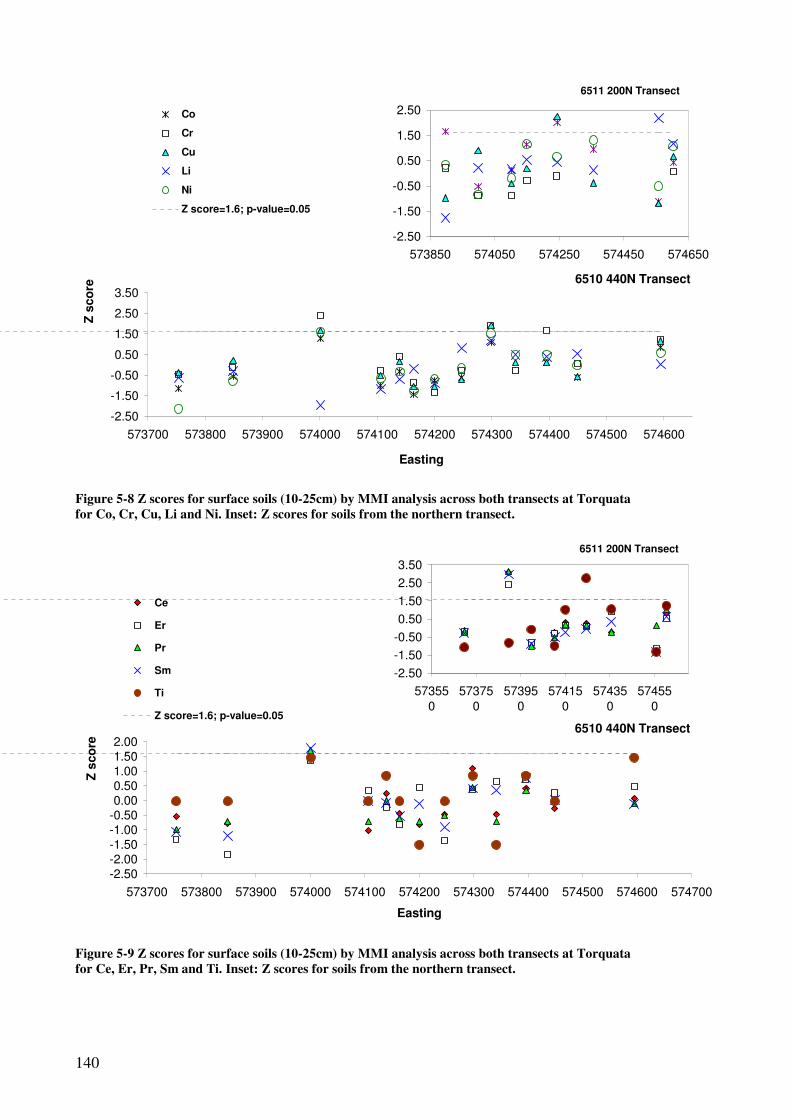
140

6510 440N Transect

-2.50

-1.50

-0.50

0.50

1.50

2.50

3.50

573700 573800 573900 574000 574100 574200 574300 574400 574500 574600

Easting

Z s

co

re

Co

Cr

Cu

Li

Ni


6511 200N Transect

-2.50

-1.50

-0.50

0.50

1.50

2.50

573850 574050 574250 574450 574650

Figure 5-8 Z scores for surface soils (10-25cm) by MMI analysis across both transects at Torquata

for Co, Cr, Cu, Li and Ni. Inset: Z scores for soils from the northern transect.

6510 440N Transect

-2.50-2.00-1.50-1.00-0.500.000.501.001.502.00

573700 573800 573900 574000 574100 574200 574300 574400 574500 574600 574700

Easting

Z s

co

re

Ce

Er

Pr

Sm

Ti


6511 200N Transect

-2.50

-1.50

-0.50

0.50

1.50

2.50

3.50

57355

0

57375

0

57395

0

57415

0

57435

0

57455

0

Figure 5-9 Z scores for surface soils (10-25cm) by MMI analysis across both transects at Torquata

for Ce, Er, Pr, Sm and Ti. Inset: Z scores for soils from the northern transect.

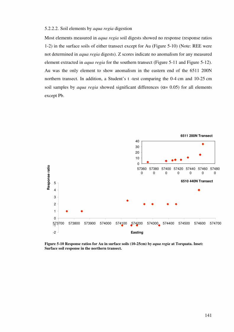
141

5.2.2.2. Soil elements by aqua regia digestion

Most elements measured in aqua regia soil digests showed no response (response ratios

1-2) in the surface soils of either transect except for Au (Figure 5-10) (Note: REE were

not determined in aqua regia digests). Z scores indicate no anomalism for any measured

element extracted in aqua regia for the southern transect (Figure 5-11 and Figure 5-12).

Au was the only element to show anomalism in the eastern end of the 6511 200N

northern transect. In addition, a Student’s t -test comparing the 0-4 cm and 10-25 cm

soil samples by aqua regia showed significant differences (α= 0.05) for all elements

except Pb.

6510 440N Transect

-2

-1

0

1

2

3

4

5

573700 573800 573900 574000 574100 574200 574300 574400 574500 574600 574700

Easting

Re

sp

on

se r

ati

o

6511 200N Transect

0

10

20

30

40

57360

0

57380

0

57400

0

57420

0

57440

0

57460

0

57480

0

Figure 5-10 Response ratios for Au in surface soils (10-25cm) by aqua regia at Torquata. Inset:

Surface soil response in the northern transect.

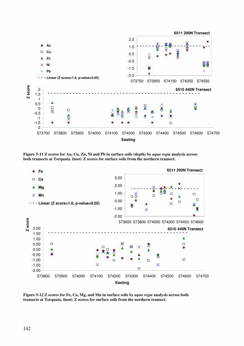
142

6510 440N Transect

-2

-1.5

-1

-0.5

0

0.5

1

1.5

2

573700 573800 573900 574000 574100 574200 574300 574400 574500 574600 574700

Easting

Z s

co

re

Au

Cu

Zn

Ni

Pb


6511 200N Transect

-2.5

-1.5

-0.5

0.5

1.5

2.5

573750 573950 574150 574350 574550

Figure 5-11 Z scores for Au, Cu, Zn, Ni and Pb in surface soils (depth) by aqua regia analysis across

both transects at Torquata. Inset: Z scores for surface soils from the northern transect.

6510 440N Transect

-2.00

-1.50

-1.00

-0.50

0.00

0.50

1.00

1.50

2.00

573800 573900 574000 574100 574200 574300 574400 574500 574600 574700

Easting

Z s

co

re

Fe

Ca

Mg

Mn


6511 200N Transect

-2.00

-1.00

0.00

1.00

2.00

3.00

573600 573800 574000 574200 574400 574600

Figure 5-12 Z scores for Fe, Ca, Mg, and Mn in surface soils by aqua regia analysis across both

transects at Torquata. Inset: Z scores for surface soils from the northern transect.

143

5.2.2.3. Trace element distribution with soil depth

Figure 5-13 shows the variation in Au concentration with soil depth for both the <2 mm

(fine) and >2 mm (coarse) soil fractions at Torquata. Firstly, there are no statistical

differences in Au concentration between the fine and coarse fractions of soil for any of

the soil pits. Secondly, both soil pits at the western end of the two transects show no

change in concentration with depth in either coarse or fine soil fractions. The soils from

the soil pits in the 6511 200N northern transect produced higher concentrations of Au

than the soil pits from the southern transect. Furthermore, the two soil pits in the eastern

end of the northern transect show a general trend of increasing Au concentration with

depth. The increasing Au with soil depth in these pits could be associated with increase

in calcrete nodules observed in the pits. Linear regression of pooled soil pit data for Au

and Ca in the coarse fraction shows a significant correlation between these two elements

when the soil pit showing anomalous Au is removed as an outlier (Figure 5-18). In

contrast, there was no relationship between Au and Ca using the data for the fine soil

fraction. There were no statistically significant differences for other elements measured

between soil depths for both fine and coarse soil fractions (Figure 5-14- Figure 5-17).

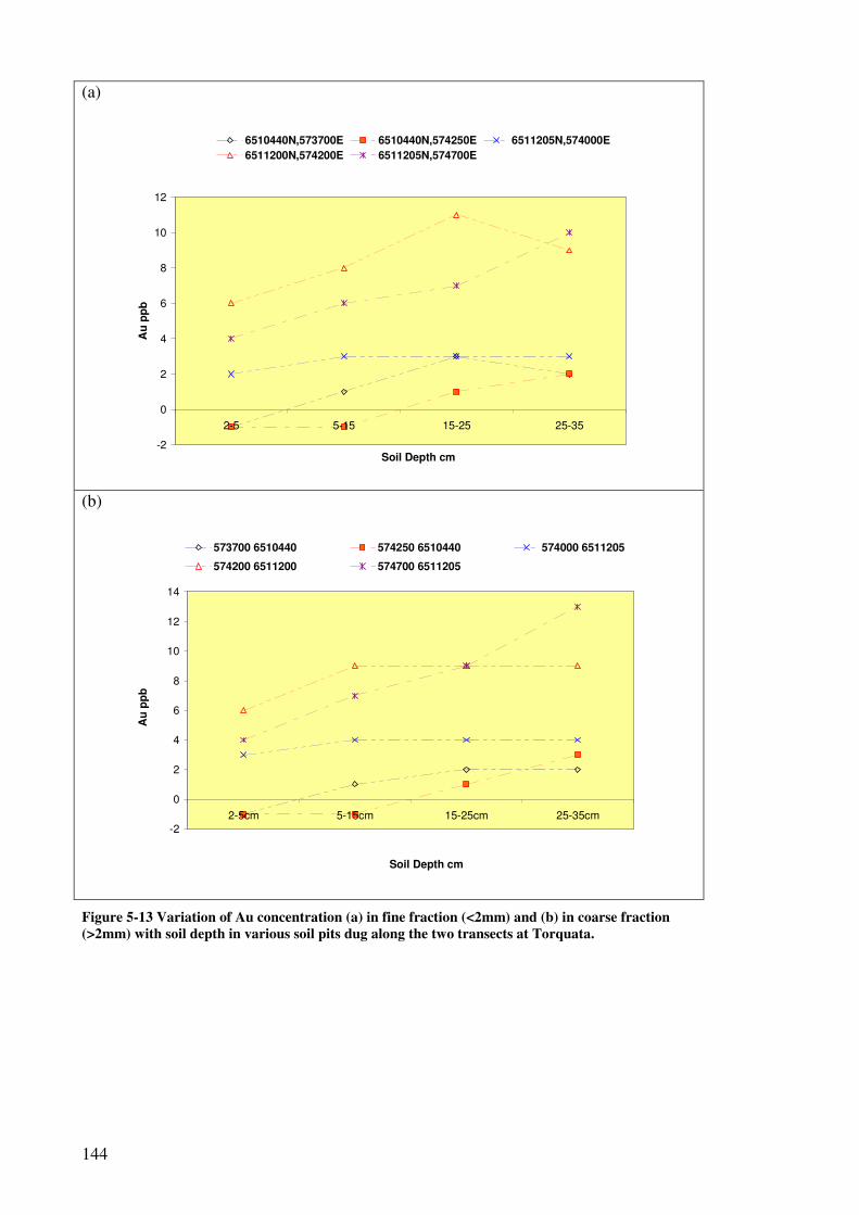
144

(a)

-2

0

2

4

6

8

10

12

2-5 5-15 15-25 25-35

Soil Depth cm

Au

pp

b6510440N,573700E 6510440N,574250E 6511205N,574000E

6511200N,574200E 6511205N,574700E

(b)

-2

0

2

4

6

8

10

12

14

2-5cm 5-15cm 15-25cm 25-35cm

Soil Depth cm

Au

pp

b

573700 6510440 574250 6510440 574000 6511205

574200 6511200 574700 6511205

Figure 5-13 Variation of Au concentration (a) in fine fraction (<2mm) and (b) in coarse fraction

(>2mm) with soil depth in various soil pits dug along the two transects at Torquata.

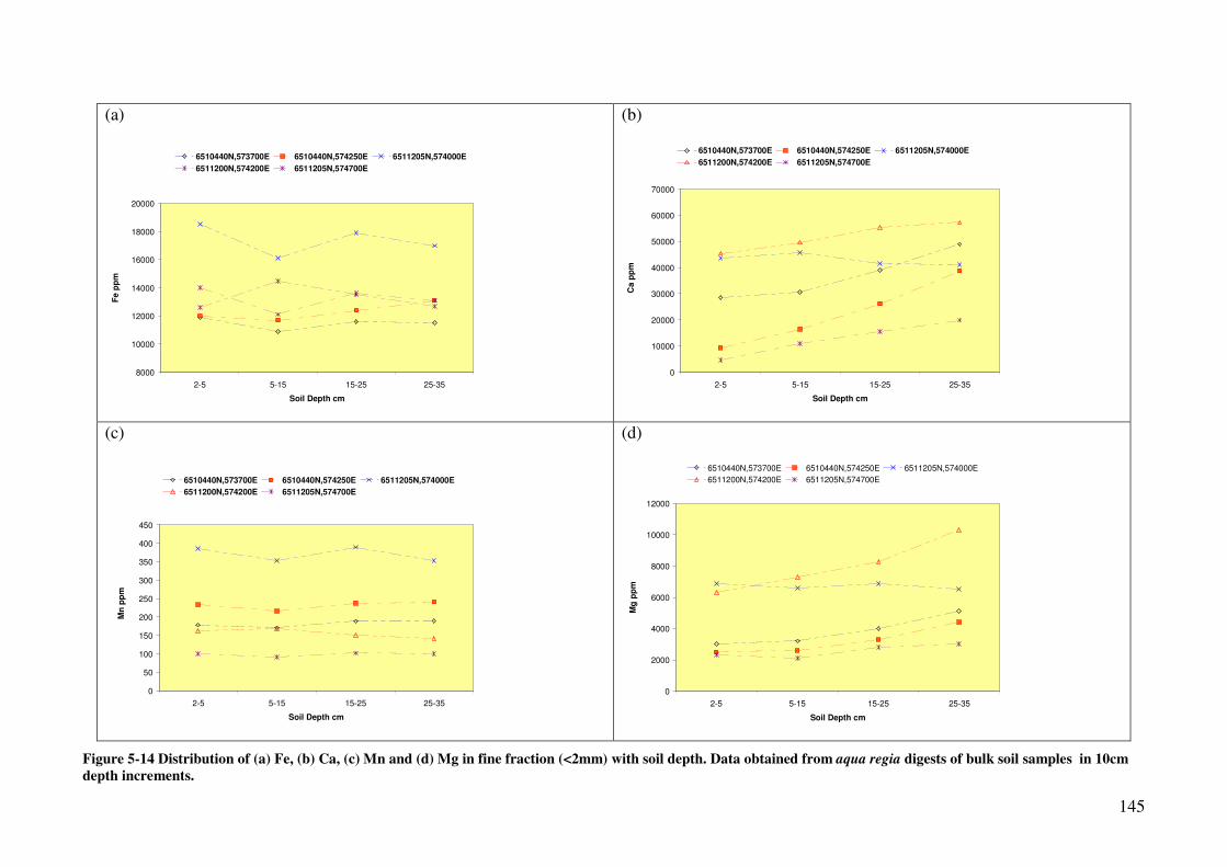
145

(a)

8000

10000

12000

14000

16000

18000

20000

2-5 5-15 15-25 25-35

Soil Depth cm

Fe

pp

m

6510440N,573700E 6510440N,574250E 6511205N,574000E

6511200N,574200E 6511205N,574700E

(b)

0

10000

20000

30000

40000

50000

60000

70000

2-5 5-15 15-25 25-35

Soil Depth cm

Ca

pp

m

6510440N,573700E 6510440N,574250E 6511205N,574000E

6511200N,574200E 6511205N,574700E

(c)

0

50

100

150

200

250

300

350

400

450

2-5 5-15 15-25 25-35

Soil Depth cm

Mn

pp

m

6510440N,573700E 6510440N,574250E 6511205N,574000E

6511200N,574200E 6511205N,574700E

(d)

0

2000

4000

6000

8000

10000

12000

2-5 5-15 15-25 25-35

Soil Depth cm

Mg

pp

m

6510440N,573700E 6510440N,574250E 6511205N,574000E

6511200N,574200E 6511205N,574700E

Figure 5-14 Distribution of (a) Fe, (b) Ca, (c) Mn and (d) Mg in fine fraction (<2mm) with soil depth. Data obtained from aqua regia digests of bulk soil samples in 10cm

depth increments.

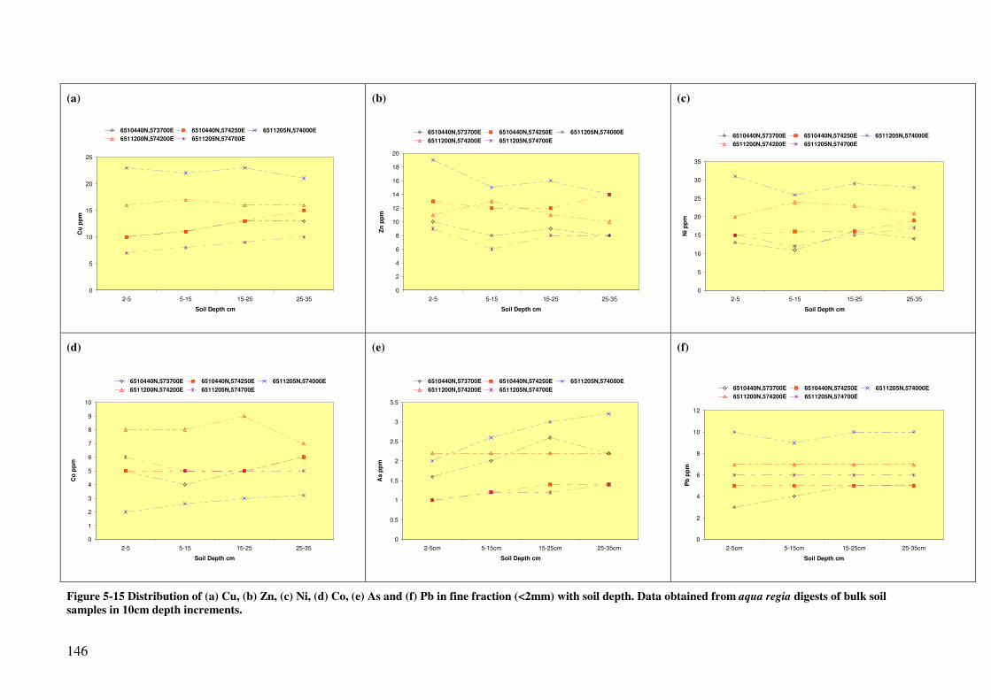
146

(a)

0

5

10

15

20

25

2-5 5-15 15-25 25-35

Soil Depth cm

Cu

pp

m

6510440N,573700E 6510440N,574250E 6511205N,574000E

6511200N,574200E 6511205N,574700E

(b)

0

2

4

6

8

10

12

14

16

18

20

2-5 5-15 15-25 25-35

Soil Depth cm

Zn

pp

m

6510440N,573700E 6510440N,574250E 6511205N,574000E

6511200N,574200E 6511205N,574700E

(c)

0

5

10

15

20

25

30

35

2-5 5-15 15-25 25-35

Soil Depth cm

Ni

pp

m

6510440N,573700E 6510440N,574250E 6511205N,574000E

6511200N,574200E 6511205N,574700E

(d)

0

1

2

3

4

5

6

7

8

9

10

2-5 5-15 15-25 25-35

Soil Depth cm

Co

pp

m

6510440N,573700E 6510440N,574250E 6511205N,574000E

6511200N,574200E 6511205N,574700E

(e)

0

0.5

1

1.5

2

2.5

3

3.5

2-5cm 5-15cm 15-25cm 25-35cm

Soil Depth cm

As p

pm

6510440N,573700E 6510440N,574250E 6511205N,574000E

6511200N,574200E 6511205N,574700E

(f)

0

2

4

6

8

10

12

2-5cm 5-15cm 15-25cm 25-35cm

Soil Depth cm

Pb

pp

m

6510440N,573700E 6510440N,574250E 6511205N,574000E

6511200N,574200E 6511205N,574700E

Figure 5-15 Distribution of (a) Cu, (b) Zn, (c) Ni, (d) Co, (e) As and (f) Pb in fine fraction (<2mm) with soil depth. Data obtained from aqua regia digests of bulk soil

samples in 10cm depth increments.

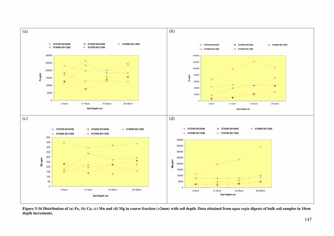
147

(a)

0

5000

10000

15000

20000

25000

30000

2-5cm 5-15cm 15-25cm 25-35cm

Soil Depth cm

Fe p

pm

573700 6510440 574250 6510440 574000 6511205

574200 6511200 574700 6511205

(b)

0

20000

40000

60000

80000

100000

120000

140000

2-5cm 5-15cm 15-25cm 25-35cm

Soil Depth cm

Ca p

pm

573700 6510440 574250 6510440 574000 6511205

574200 6511200 574700 6511205

(c)

0

50

100

150

200

250

300

350

400

450

500

2-5cm 5-15cm 15-25cm 25-35cm

Soil Depth cm

Mn

pp

m

573700 6510440 574250 6510440 574000 6511205

574200 6511200 574700 6511205

(d)

0

5000

10000

15000

20000

25000

30000

35000

40000

2-5cm 5-15cm 15-25cm 25-35cm

Soil Depth cm

Mg

pp

m

573700 6510440 574250 6510440 574000 6511205

574200 6511200 574700 6511205

Figure 5-16 Distribution of (a) Fe, (b) Ca, (c) Mn and (d) Mg in coarse fraction (>2mm) with soil depth. Data obtained from aqua regia digests of bulk soil samples in 10cm

depth increments.

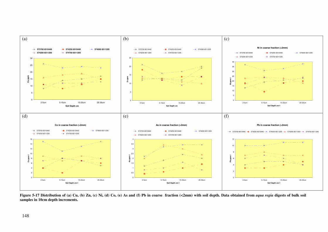
148

(a)

0

5

10

15

20

25

30

2-5cm 5-15cm 15-25cm 25-35cm

Soil Depth cm

Cu

pp

m

573700 6510440 574250 6510440 574000 6511205

574200 6511200 574700 6511205

(b)

0

5

10

15

20

25

2-5cm 5-15cm 15-25cm 25-35cm

Soil Depth cm

Zn

pp

m

573700 6510440 574250 6510440 574000 6511205

574200 6511200 574700 6511205

(c)

Ni in coarse fraction (>2mm)

0

5

10

15

20

25

30

35

40

2-5cm 5-15cm 15-25cm 25-35cm

Soil Depth cm-1

Ni p

pm

-1

573700 6510440 574250 6510440 574000 6511205

574200 6511200 574700 6511205

(d)

Co in coarse fraction (>2mm)

0

2

4

6

8

10

12

14

16

2-5cm 5-15cm 15-25cm 25-35cm

Soil Depth cm-1

Co

pp

m-1

573700 6510440 574250 6510440 574000 6511205

574200 6511200 574700 6511205

(e)

As in coarse fraction (>2mm)

0

0.5

1

1.5

2

2.5

3

3.5

4

2-5cm 5-15cm 15-25cm 25-35cm

Soil Depth cm-1

As

pp

m-1

573700 6510440 574250 6510440 574000 6511205

574200 6511200 574700 6511205

(f)

Pb in coarse fraction (>2mm)

0

2

4

6

8

10

12

2-5cm 5-15cm 15-25cm 25-35cm

Soil Depth cm-1

Pb

pp

m-1

573700 6510440 574250 6510440 574000 6511205 574200 6511200 574700 6511205

Figure 5-17 Distribution of (a) Cu, (b) Zn, (c) Ni, (d) Co, (e) As and (f) Pb in coarse fraction (<2mm) with soil depth. Data obtained from aqua regia digests of bulk soil

samples in 10cm depth increments.

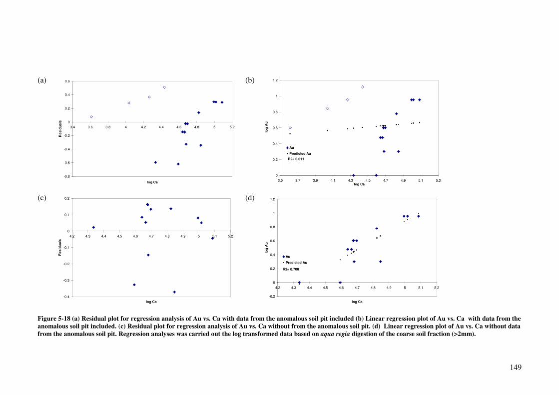
149

(a)

-0.8

-0.6

-0.4

-0.2

0

0.2

0.4

0.6

3.4 3.6 3.8 4 4.2 4.4 4.6 4.8 5 5.2

log Ca

Re

sid

ua

ls

(b)

0

0.2

0.4

0.6

0.8

1

1.2

3.5 3.7 3.9 4.1 4.3 4.5 4.7 4.9 5.1 5.3log Ca

log

Au

Au

Predicted Au

R2= 0.011

(c)

-0.4

-0.3

-0.2

-0.1

0

0.1

0.2

4.2 4.3 4.4 4.5 4.6 4.7 4.8 4.9 5 5.1 5.2

log Ca

Re

sid

uals

(d)

-0.2

0

0.2

0.4

0.6

0.8

1

1.2

4.2 4.3 4.4 4.5 4.6 4.7 4.8 4.9 5 5.1 5.2

log Ca

log

Au

Au

Predicted Au

R2= 0.708

Figure 5-18 (a) Residual plot for regression analysis of Au vs. Ca with data from the anomalous soil pit included (b) Linear regression plot of Au vs. Ca with data from the

anomalous soil pit included. (c) Residual plot for regression analysis of Au vs. Ca without from the anomalous soil pit. (d) Linear regression plot of Au vs. Ca without data

from the anomalous soil pit. Regression analyses was carried out the log transformed data based on aqua regia digestion of the coarse soil fraction (>2mm).

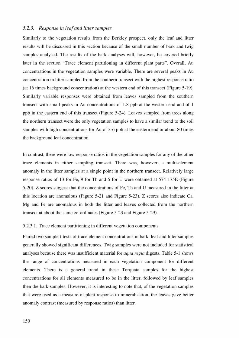
150

5.2.3. Response in leaf and litter samples

Similarly to the vegetation results from the Berkley prospect, only the leaf and litter

results will be discussed in this section because of the small number of bark and twig

samples analysed. The results of the bark analyses will, however, be covered briefly

later in the section “Trace element partitioning in different plant parts”. Overall, Au

concentrations in the vegetation samples were variable. There are several peaks in Au

concentration in litter sampled from the southern transect with the highest response ratio

(at 16 times background concentration) at the western end of this transect (Figure 5-19).

Similarly variable responses were obtained from leaves sampled from the southern

transect with small peaks in Au concentrations of 1.8 ppb at the western end and of 1

ppb in the eastern end of this transect (Figure 5-24). Leaves sampled from trees along

the northern transect were the only vegetation samples to have a similar trend to the soil

samples with high concentrations for Au of 3-6 ppb at the eastern end or about 80 times

the background leaf concentration.

In contrast, there were low response ratios in the vegetation samples for any of the other

trace elements in either sampling transect. There was, however, a multi-element

anomaly in the litter samples at a single point in the northern transect. Relatively large

response ratios of 13 for Fe, 9 for Th and 5 for U were obtained at 574 175E (Figure

5-20). Z scores suggest that the concentrations of Fe, Th and U measured in the litter at

this location are anomalous (Figure 5-21 and Figure 5-23). Z scores also indicate Ca,

Mg and Fe are anomalous in both the litter and leaves collected from the northern

transect at about the same co-ordinates (Figure 5-23 and Figure 5-29).

5.2.3.1. Trace element partitioning in different vegetation components

Paired two sample t-tests of trace element concentrations in bark, leaf and litter samples

generally showed significant differences. Twig samples were not included for statistical

analyses because there was insufficient material for aqua regia digests. Table 5-1 shows

the range of concentrations measured in each vegetation component for different

elements. There is a general trend in these Torquata samples for the highest

concentrations for all elements measured to be in the litter, followed by leaf samples

then the bark samples. However, it is interesting to note that, of the vegetation samples

that were used as a measure of plant response to mineralisation, the leaves gave better

anomaly contrast (measured by response ratios) than litter.

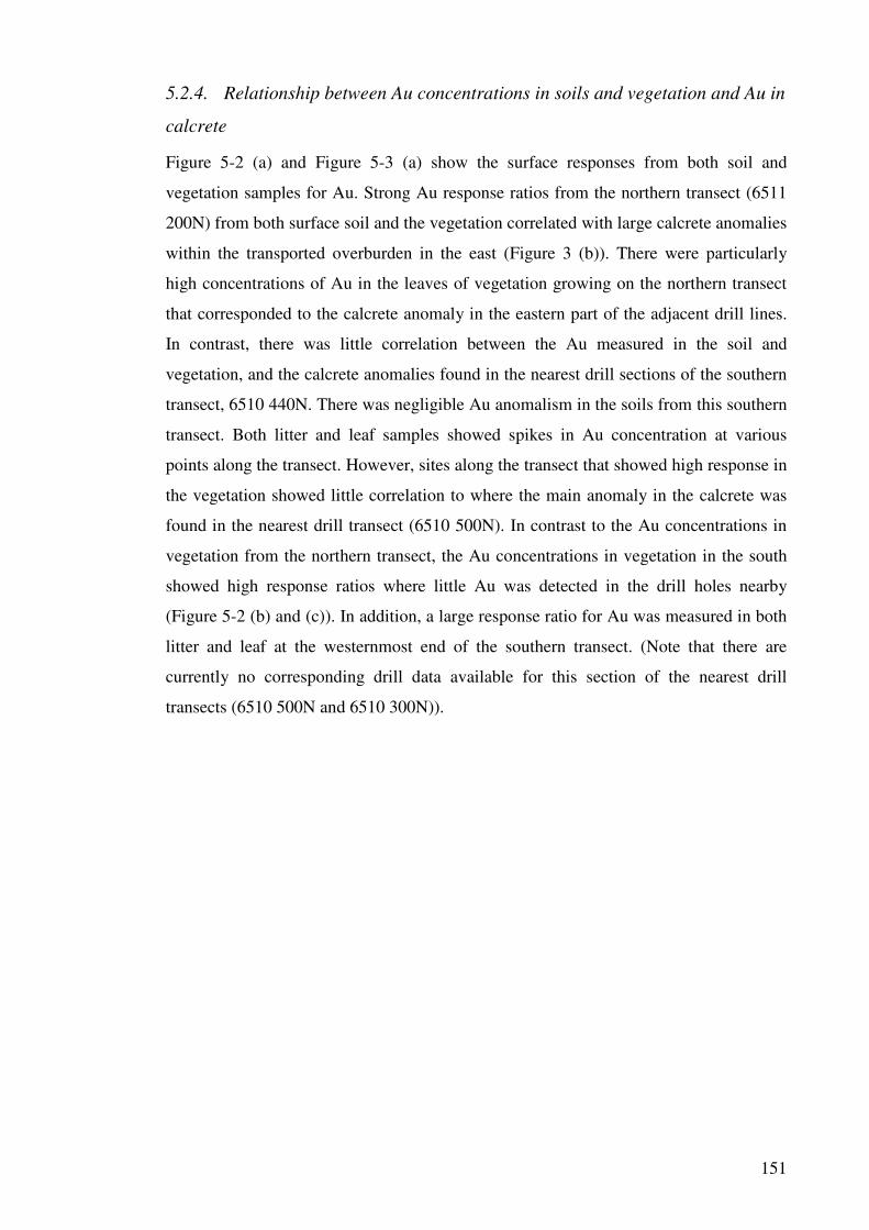
151

5.2.4. Relationship between Au concentrations in soils and vegetation and Au in

calcrete

Figure 5-2 (a) and Figure 5-3 (a) show the surface responses from both soil and

vegetation samples for Au. Strong Au response ratios from the northern transect (6511

200N) from both surface soil and the vegetation correlated with large calcrete anomalies

within the transported overburden in the east (Figure 3 (b)). There were particularly

high concentrations of Au in the leaves of vegetation growing on the northern transect

that corresponded to the calcrete anomaly in the eastern part of the adjacent drill lines.

In contrast, there was little correlation between the Au measured in the soil and

vegetation, and the calcrete anomalies found in the nearest drill sections of the southern

transect, 6510 440N. There was negligible Au anomalism in the soils from this southern

transect. Both litter and leaf samples showed spikes in Au concentration at various

points along the transect. However, sites along the transect that showed high response in

the vegetation showed little correlation to where the main anomaly in the calcrete was

found in the nearest drill transect (6510 500N). In contrast to the Au concentrations in

vegetation from the northern transect, the Au concentrations in vegetation in the south

showed high response ratios where little Au was detected in the drill holes nearby

(Figure 5-2 (b) and (c)). In addition, a large response ratio for Au was measured in both

litter and leaf at the westernmost end of the southern transect. (Note that there are

currently no corresponding drill data available for this section of the nearest drill

transects (6510 500N and 6510 300N)).

152

6510 440N Transect

0

2

4

6

8

10

12

14

16

18

20

573600 573800 574000 574200 574400 574600

Easting

Re

sp

on

se r

ati

o

Au

Cr

Cd

6511 200N Transect

05

101520253035

573500 574000 574500 575000

0

10

20

30

40

50

60

Cd

Re

sp

on

se

rati

o

Figure 5-19 Response ratios for Au, Cr and Cd measured in litter at Torquata along both transects.

Inset: Litter response ratios for northern transect.

6510 440N Transect

0.0

0.5

1.0

1.5

2.0

2.5

3.0

3.5

573650 573750 573850 573950 574050 574150 574250 574350 574450 574550 574650

Easting

Resp

on

se

rati

o

Th

U

Mn

Fe

6511 200N Transect

0

5

10

15

573500 574000 574500 575000

Figure 5-20 Response ratios for Th, U, Mn and Fe measured in litter at Torquata along both

transects. Inset: Response ratios for elements measured in litter sampled from the northern

transect.

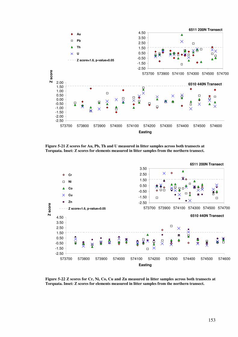
153

6510 440N Transect

-2.50-2.00-1.50-1.00-0.500.000.501.001.502.00

573700 573800 573900 574000 574100 574200 574300 574400 574500 574600

Easting

Z s

co

re

Au

Pb

Th

U

Z score=1.6, p-value=0.05

6511 200N Transect

-2.50

-1.50

-0.50

0.50

1.50

2.50

3.50

4.50

573700 573900 574100 574300 574500 574700

Figure 5-21 Z scores for Au, Pb, Th and U measured in litter samples across both transects at

Torquata. Inset: Z scores for elements measured in litter samples from the northern transect.

6510 440N Transect

-2.50

-1.50

-0.50

0.50

1.50

2.50

3.50

4.50

573700 573800 573900 574000 574100 574200 574300 574400 574500 574600

Easting

Z s

co

re

Cr

Ni

Co

Cu

Zn

Z score=1.6, p-value=0.05

6511 200N Transect

-2.50

-1.50

-0.50

0.50

1.50

2.50

3.50

573700 573900 574100 574300 574500 574700

Figure 5-22 Z scores for Cr, Ni, Co, Cu and Zn measured in litter samples across both transects at


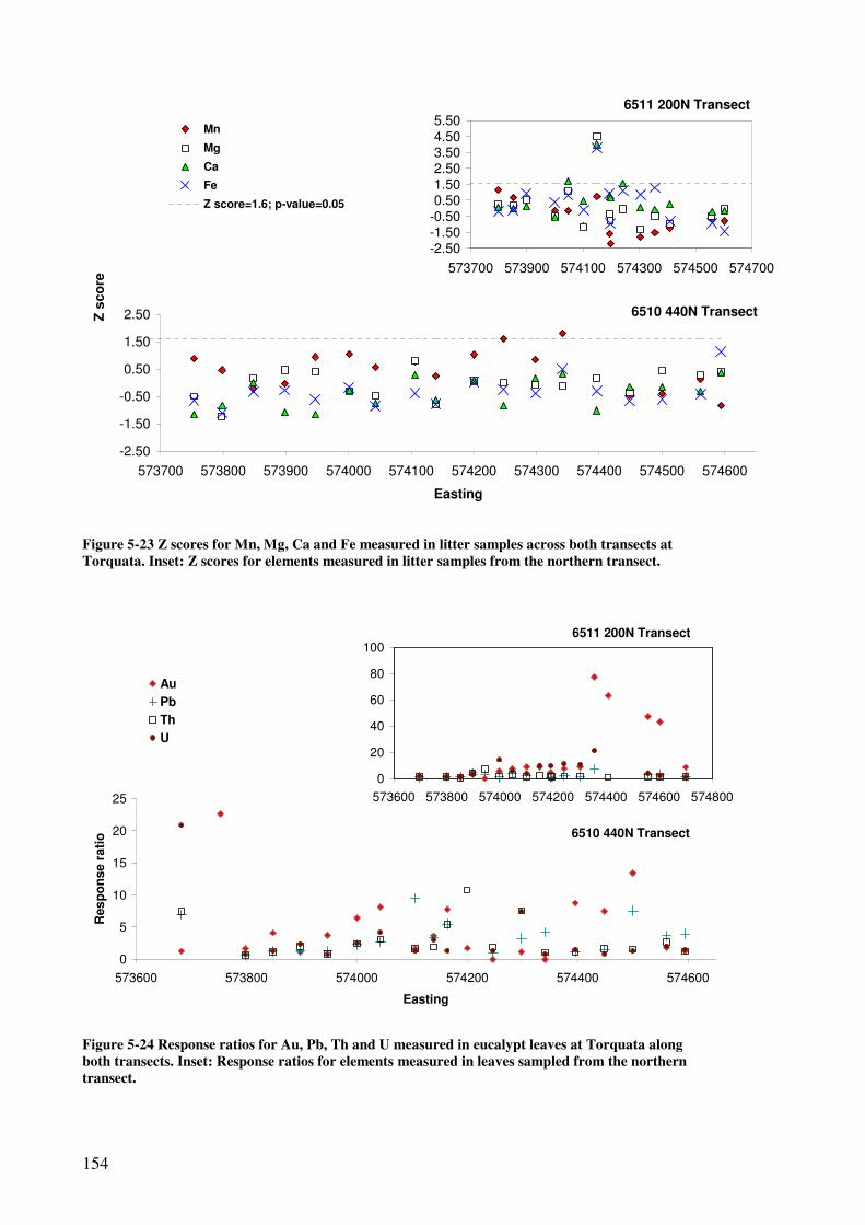
154

6510 440N Transect

-2.50

-1.50

-0.50

0.50

1.50

2.50

573700 573800 573900 574000 574100 574200 574300 574400 574500 574600

Easting

Z s

co

re

Mn

Mg

Ca

Fe


6511 200N Transect

-2.50-1.50-0.500.501.502.503.504.505.50

573700 573900 574100 574300 574500 574700

Figure 5-23 Z scores for Mn, Mg, Ca and Fe measured in litter samples across both transects at


6510 440N Transect

0

5

10

15

20

25

573600 573800 574000 574200 574400 574600

Easting

Res

po

ns

e r

ati

o

Au

Pb

Th

U

6511 200N Transect

0

20

40

60

80

100

573600 573800 574000 574200 574400 574600 574800

Figure 5-24 Response ratios for Au, Pb, Th and U measured in eucalypt leaves at Torquata along

both transects. Inset: Response ratios for elements measured in leaves sampled from the northern

transect.

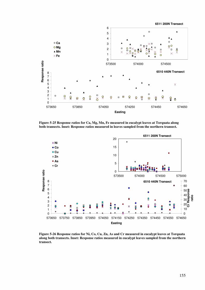
155

6510 440N Transect

0

1

2

3

4

5

6

7

8

573650 573850 574050 574250 574450 574650

Easting

Re

sp

on

se r

ati

oCa

Mg

Mn

Fe

6511 200N Transect

0

1

2

3

4

5

6

573500 574000 574500

Figure 5-25 Response ratios for Ca, Mg, Mn, Fe measured in eucalypt leaves at Torquata along

both transects. Inset: Response ratios measured in leaves sampled from the northern transect.

6510 440N Transect

0

1

2

3

4

5

6

7

8

573650 573750 573850 573950 574050 574150 574250 574350 574450 574550 574650

Easting

Re

sp

on

se r

ati

o

0

10

20

30

40

50

60

70

Cr

Re

sp

on

se

rati

o

Ni

Co

Cu

Zn

As

Cr

6511 200N Transect

0

5

10

15

20

573500 574000 574500 575000

Figure 5-26 Response ratios for Ni, Co, Cu, Zn, As and Cr measured in eucalypt leaves at Torquata

along both transects. Inset: Response ratios measured in eucalypt leaves sampled from the northern

transect.

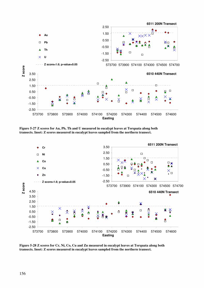
156

6510 440N Transect

-2.50

-1.50

-0.50

0.50

1.50

2.50

3.50

573700 573800 573900 574000 574100 574200 574300 574400 574500 574600

Easting

Z s

co

re

Au

Pb

Th

U


6511 200N Transect

-2.50

-1.50

-0.50

0.50

1.50

2.50

573700 573900 574100 574300 574500 574700

Figure 5-27 Z scores for Au, Pb, Th and U measured in eucalypt leaves at Torquata along both

transects. Inset: Z scores measured in eucalypt leaves sampled from the northern transect.

6510 440N Transect

-2.50

-1.50

-0.50

0.50

1.50

2.50

3.50

4.50

573700 573800 573900 574000 574100 574200 574300 574400 574500 574600Easting

Z s

co

re

Cr

Ni

Co

Cu

Zn


6511 200N Transect

-2.50

-1.50

-0.50

0.50

1.50

2.50

3.50

573700 573900 574100 574300 574500 574700

Figure 5-28 Z scores for Cr, Ni, Co, Cu and Zn measured in eucalypt leaves at Torquata along both


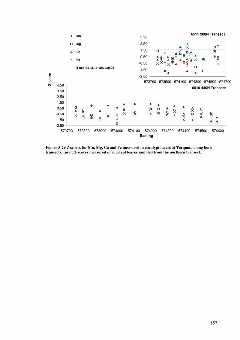
157

6510 440N Transect

-2.50

-1.50

-0.50

0.50

1.50

2.50

3.50

4.50

573700 573800 573900 574000 574100 574200 574300 574400 574500 574600

Easting

Z s

co

re

Mn

Mg

Ca

Fe


6511 200N Transect

-2.50

-1.50

-0.50

0.50

1.50

2.50

3.50

573700 573900 574100 574300 574500 574700

Figure 5-29 Z scores for Mn, Mg, Ca and Fe measured in eucalypt leaves at Torquata along both


158

5.2.5. Regression analyses

Au measured in the soil and vegetation samples from both transects does not co-vary

with any other trace element. Correlation analyses confirm that the Au measured in each

sample type is independent of other trace elements (Table 5-2-Table 5-5). There is,

however, a weak correlation between Au and Li in the MMI soil samples (Table 5-2).

Linear regression modelling showed that Au and Li are significantly related at a

significance value of <1% (p-value=0.0009), despite the low R value. Surprisingly, the

Au in the soil samples showed poor correlation with total/MMI soil Ca despite the fact

that most of the sub-surface Au (and source of Au in the soils) is associated with

calcrete at Torquata. There is also a weak correlation between Au and Ca measured in

leaf samples at a significance value of <10% (p-value=0.0537) (Figure 5-31).

Further, regression analyses between soil and plant samples showed no general trend for

most elements (Table 5-6). Au measured in leaves was positively correlated with both

the MMI and aqua regia soil Au. Further, a particularly strong correlation was observed

between the MMI and aqua regia soil samples for Au (R=0.94; p-value<0.001) (Also

see Figure 5-30). There were also statistically significant correlations between

concentrations in soils (10-25 cm depth) and vegetation for Zn, Ca, Mg and Fe (See

Table 5-6).

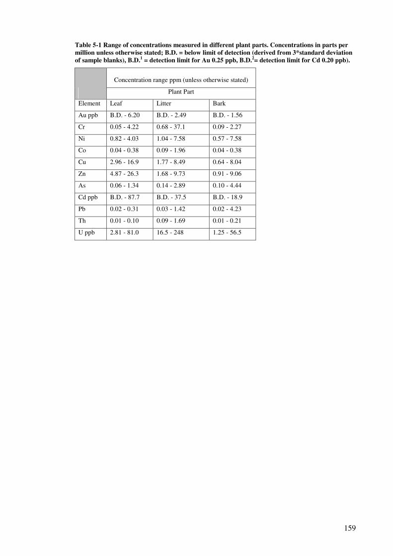
159

Table 5-1 Range of concentrations measured in different plant parts. Concentrations in parts per

million unless otherwise stated; B.D. = below limit of detection (derived from 3*standard deviation

of sample blanks), B.D.1 = detection limit for Au 0.25 ppb, B.D.

2= detection limit for Cd 0.20 ppb).

Concentration range ppm (unless otherwise stated)

Plant Part

Element Leaf Litter Bark

Au ppb B.D. - 6.20 B.D. - 2.49 B.D. - 1.56

Cr 0.05 - 4.22 0.68 - 37.1 0.09 - 2.27

Ni 0.82 - 4.03 1.04 - 7.58 0.57 - 7.58

Co 0.04 - 0.38 0.09 - 1.96 0.04 - 0.38

Cu 2.96 - 16.9 1.77 - 8.49 0.64 - 8.04

Zn 4.87 - 26.3 1.68 - 9.73 0.91 - 9.06

As 0.06 - 1.34 0.14 - 2.89 0.10 - 4.44

Cd ppb B.D. - 87.7 B.D. - 37.5 B.D. - 18.9

Pb 0.02 - 0.31 0.03 - 1.42 0.02 - 4.23

Th 0.01 - 0.10 0.09 - 1.69 0.01 - 0.21

U ppb 2.81 - 81.0 16.5 - 248 1.25 - 56.5

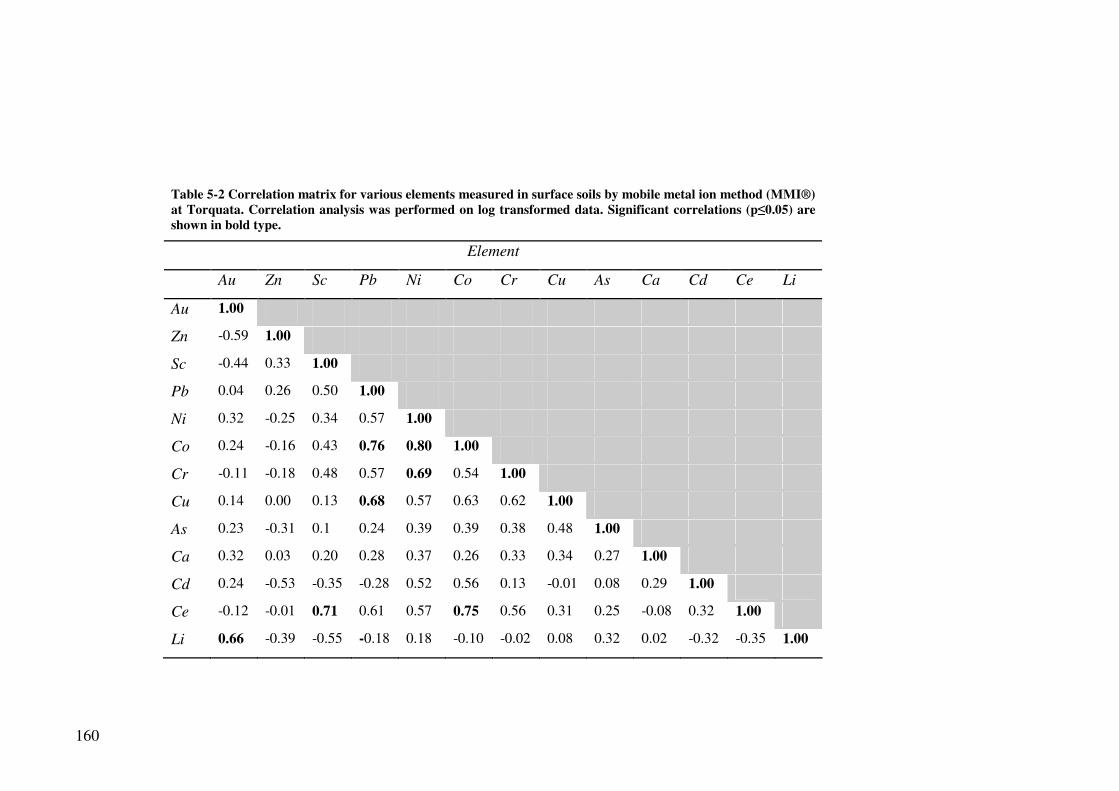
160

Table 5-2 Correlation matrix for various elements measured in surface soils by mobile metal ion method (MMI®)

at Torquata. Correlation analysis was performed on log transformed data. Significant correlations (p≤0.05) are

shown in bold type.

Element

Au Zn Sc Pb Ni Co Cr Cu As Ca Cd Ce Li

Au 1.00

Zn -0.59 1.00

Sc -0.44 0.33 1.00

Pb 0.04 0.26 0.50 1.00

Ni 0.32 -0.25 0.34 0.57 1.00

Co 0.24 -0.16 0.43 0.76 0.80 1.00

Cr -0.11 -0.18 0.48 0.57 0.69 0.54 1.00

Cu 0.14 0.00 0.13 0.68 0.57 0.63 0.62 1.00

As 0.23 -0.31 0.1 0.24 0.39 0.39 0.38 0.48 1.00

Ca 0.32 0.03 0.20 0.28 0.37 0.26 0.33 0.34 0.27 1.00

Cd 0.24 -0.53 -0.35 -0.28 0.52 0.56 0.13 -0.01 0.08 0.29 1.00

Ce -0.12 -0.01 0.71 0.61 0.57 0.75 0.56 0.31 0.25 -0.08 0.32 1.00

Li 0.66 -0.39 -0.55 -0.18 0.18 -0.10 -0.02 0.08 0.32 0.02 -0.32 -0.35 1.00

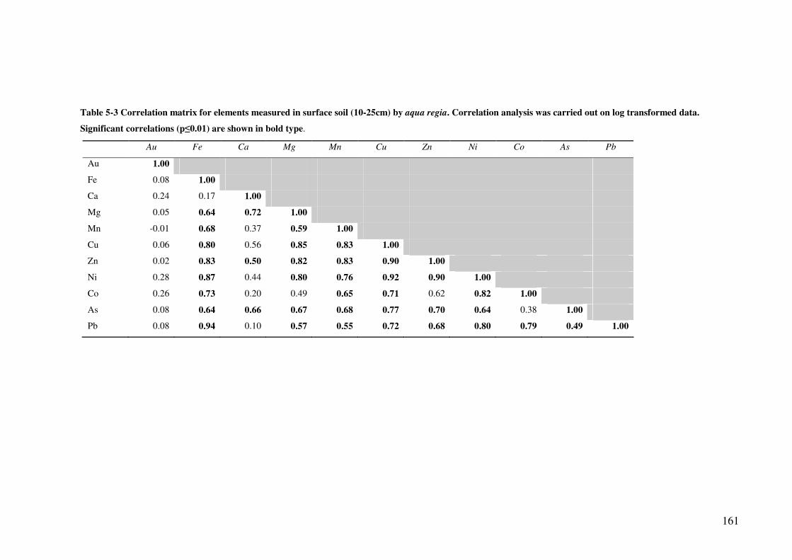
161

Table 5-3 Correlation matrix for elements measured in surface soil (10-25cm) by aqua regia. Correlation analysis was carried out on log transformed data.

Significant correlations (p≤0.01) are shown in bold type.

Au Fe Ca Mg Mn Cu Zn Ni Co As Pb

Au 1.00

Fe 0.08 1.00

Ca 0.24 0.17 1.00

Mg 0.05 0.64 0.72 1.00

Mn -0.01 0.68 0.37 0.59 1.00

Cu 0.06 0.80 0.56 0.85 0.83 1.00

Zn 0.02 0.83 0.50 0.82 0.83 0.90 1.00

Ni 0.28 0.87 0.44 0.80 0.76 0.92 0.90 1.00

Co 0.26 0.73 0.20 0.49 0.65 0.71 0.62 0.82 1.00

As 0.08 0.64 0.66 0.67 0.68 0.77 0.70 0.64 0.38 1.00

Pb 0.08 0.94 0.10 0.57 0.55 0.72 0.68 0.80 0.79 0.49 1.00

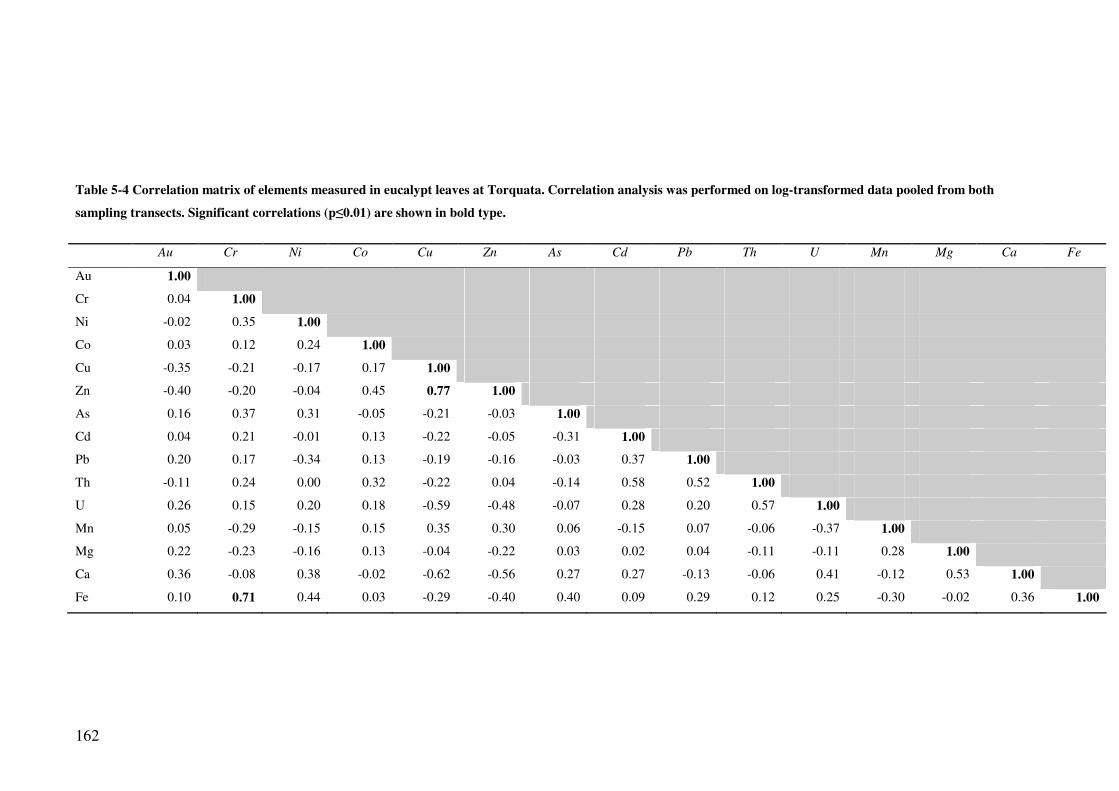
162

Table 5-4 Correlation matrix of elements measured in eucalypt leaves at Torquata. Correlation analysis was performed on log-transformed data pooled from both

sampling transects. Significant correlations (p≤0.01) are shown in bold type.

Au Cr Ni Co Cu Zn As Cd Pb Th U Mn Mg Ca Fe

Au 1.00

Cr 0.04 1.00

Ni -0.02 0.35 1.00

Co 0.03 0.12 0.24 1.00

Cu -0.35 -0.21 -0.17 0.17 1.00

Zn -0.40 -0.20 -0.04 0.45 0.77 1.00

As 0.16 0.37 0.31 -0.05 -0.21 -0.03 1.00

Cd 0.04 0.21 -0.01 0.13 -0.22 -0.05 -0.31 1.00

Pb 0.20 0.17 -0.34 0.13 -0.19 -0.16 -0.03 0.37 1.00

Th -0.11 0.24 0.00 0.32 -0.22 0.04 -0.14 0.58 0.52 1.00

U 0.26 0.15 0.20 0.18 -0.59 -0.48 -0.07 0.28 0.20 0.57 1.00

Mn 0.05 -0.29 -0.15 0.15 0.35 0.30 0.06 -0.15 0.07 -0.06 -0.37 1.00

Mg 0.22 -0.23 -0.16 0.13 -0.04 -0.22 0.03 0.02 0.04 -0.11 -0.11 0.28 1.00

Ca 0.36 -0.08 0.38 -0.02 -0.62 -0.56 0.27 0.27 -0.13 -0.06 0.41 -0.12 0.53 1.00

Fe 0.10 0.71 0.44 0.03 -0.29 -0.40 0.40 0.09 0.29 0.12 0.25 -0.30 -0.02 0.36 1.00

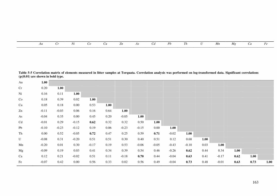
163

Table 5-5 Correlation matrix of elements measured in litter samples at Torquata. Correlation analysis was performed on log-transformed data. Significant correlations

(p≤0.01) are shown in bold type.

Au Cr Ni Co Cu Zn As Cd Pb Th U Mn Mg Ca Fe

Au 1.00

Cr 0.20 1.00

Ni 0.16 0.11 1.00

Co 0.18 0.39 0.02 1.00

Cu 0.05 0.18 0.00 0.53 1.00

Zn -0.11 -0.03 0.06 0.16 0.64 1.00

As -0.04 0.35 0.00 0.45 0.20 -0.05 1.00

Cd -0.01 0.29 -0.15 0.62 0.32 0.32 0.50 1.00

Pb -0.10 -0.23 -0.12 0.19 0.06 -0.23 -0.15 0.00 1.00

Th 0.00 0.52 -0.05 0.72 0.47 0.25 0.59 0.71 -0.02 1.00

U -0.08 0.31 -0.20 0.51 0.51 0.30 0.40 0.51 0.12 0.68 1.00

Mn -0.20 0.01 0.30 -0.17 0.19 0.53 -0.06 -0.05 -0.43 -0.10 0.03 1.00

Mg -0.09 0.19 0.03 0.41 0.34 0.39 0.54 0.46 -0.26 0.62 0.44 0.34 1.00

Ca 0.12 0.21 -0.02 0.51 0.11 -0.18 0.70 0.44 -0.04 0.63 0.41 -0.17 0.62 1.00

Fe -0.07 0.42 0.00 0.56 0.33 0.02 0.56 0.49 -0.04 0.73 0.48 -0.01 0.63 0.73 1.00

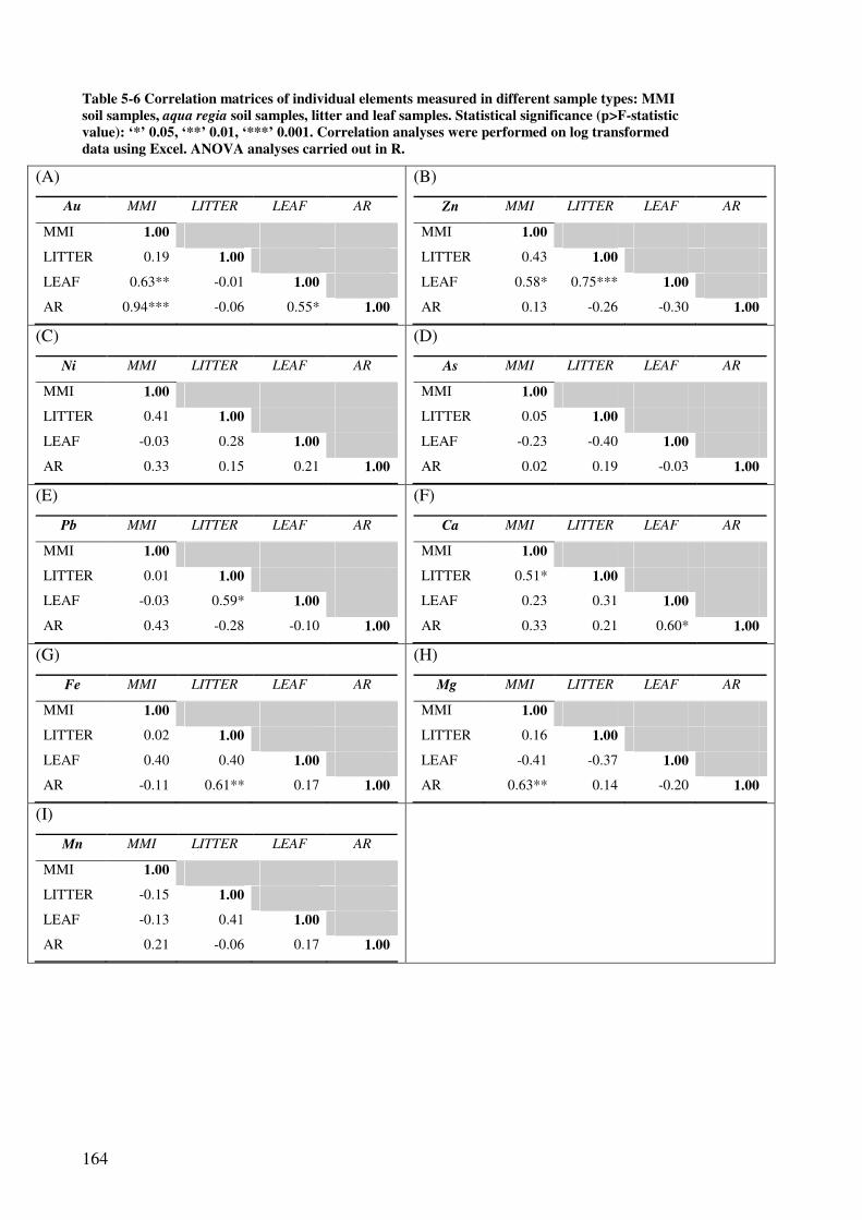
164

Table 5-6 Correlation matrices of individual elements measured in different sample types: MMI

soil samples, aqua regia soil samples, litter and leaf samples. Statistical significance (p>F-statistic

value): ‘*’ 0.05, ‘**’ 0.01, ‘***’ 0.001. Correlation analyses were performed on log transformed

data using Excel. ANOVA analyses carried out in R.

(A)

Au MMI LITTER LEAF AR

MMI 1.00

LITTER 0.19 1.00

LEAF 0.63** -0.01 1.00

AR 0.94*** -0.06 0.55* 1.00

(B)

Zn MMI LITTER LEAF AR

MMI 1.00

LITTER 0.43 1.00

LEAF 0.58* 0.75*** 1.00

AR 0.13 -0.26 -0.30 1.00

(C)

Ni MMI LITTER LEAF AR

MMI 1.00

LITTER 0.41 1.00

LEAF -0.03 0.28 1.00

AR 0.33 0.15 0.21 1.00

(D)

As MMI LITTER LEAF AR

MMI 1.00

LITTER 0.05 1.00

LEAF -0.23 -0.40 1.00

AR 0.02 0.19 -0.03 1.00

(E)

Pb MMI LITTER LEAF AR

MMI 1.00

LITTER 0.01 1.00

LEAF -0.03 0.59* 1.00

AR 0.43 -0.28 -0.10 1.00

(F)

Ca MMI LITTER LEAF AR

MMI 1.00

LITTER 0.51* 1.00

LEAF 0.23 0.31 1.00

AR 0.33 0.21 0.60* 1.00

(G)

Fe MMI LITTER LEAF AR

MMI 1.00

LITTER 0.02 1.00

LEAF 0.40 0.40 1.00

AR -0.11 0.61** 0.17 1.00

(H)

Mg MMI LITTER LEAF AR

MMI 1.00

LITTER 0.16 1.00

LEAF -0.41 -0.37 1.00

AR 0.63** 0.14 -0.20 1.00

(I)

Mn MMI LITTER LEAF AR

MMI 1.00

LITTER -0.15 1.00

LEAF -0.13 0.41 1.00

AR 0.21 -0.06 0.17 1.00

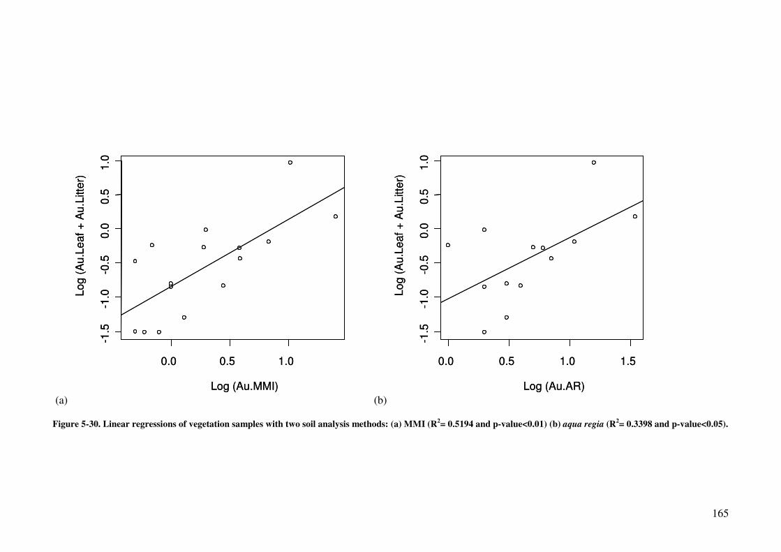
165

(a)

0.0 0.5 1.0

-1.5

-1.0

-0.5

0.0

0.5

1.0

Log (Au.MMI)

Lo

g (

Au

.Le

af

+ A

u.L

itte

r)

0.0 0.5 1.0

-1.5

-1.0

-0.5

0.0

0.5

1.0

Log (Au.MMI)

Lo

g (

Au

.Le

af

+ A

u.L

itte

r)

(b)

0.0 0.5 1.0 1.5

-1.5

-1.0

-0.5

0.0

0.5

1.0

Log (Au.AR)Lo

g (

Au

.Le

af

+ A

u.L

itte

r)

0.0 0.5 1.0 1.5

-1.5

-1.0

-0.5

0.0

0.5

1.0

Log (Au.AR)Lo

g (

Au

.Le

af

+ A

u.L

itte

r)

Figure 5-30. Linear regressions of vegetation samples with two soil analysis methods: (a) MMI (R2= 0.5194 and p-value<0.01) (b) aqua regia (R

2= 0.3398 and p-value<0.05).

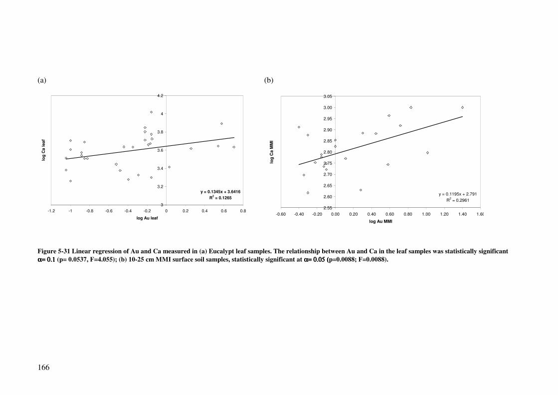
166

(a)

y = 0.1345x + 3.6416

R2 = 0.1265

3

3.2

3.4

3.6

3.8

4

4.2

-1.2 -1 -0.8 -0.6 -0.4 -0.2 0 0.2 0.4 0.6 0.8

log Au leaf

log

Ca

lea

f

(b)

y = 0.1195x + 2.791

R2 = 0.2961

2.55

2.60

2.65

2.70

2.75

2.80

2.85

2.90

2.95

3.00

3.05

-0.60 -0.40 -0.20 0.00 0.20 0.40 0.60 0.80 1.00 1.20 1.40 1.60

log Au MMI

log

Ca M

MI

Figure 5-31 Linear regression of Au and Ca measured in (a) Eucalypt leaf samples. The relationship between Au and Ca in the leaf samples was statistically significant

α= 0.1α= 0.1α= 0.1α= 0.1 (p= 0.0537, F=4.055); (b) 10-25 cm MMI surface soil samples, statistically significant at α= 0.05 (α= 0.05 (α= 0.05 (α= 0.05 (p=0.0088; F=0.0088).

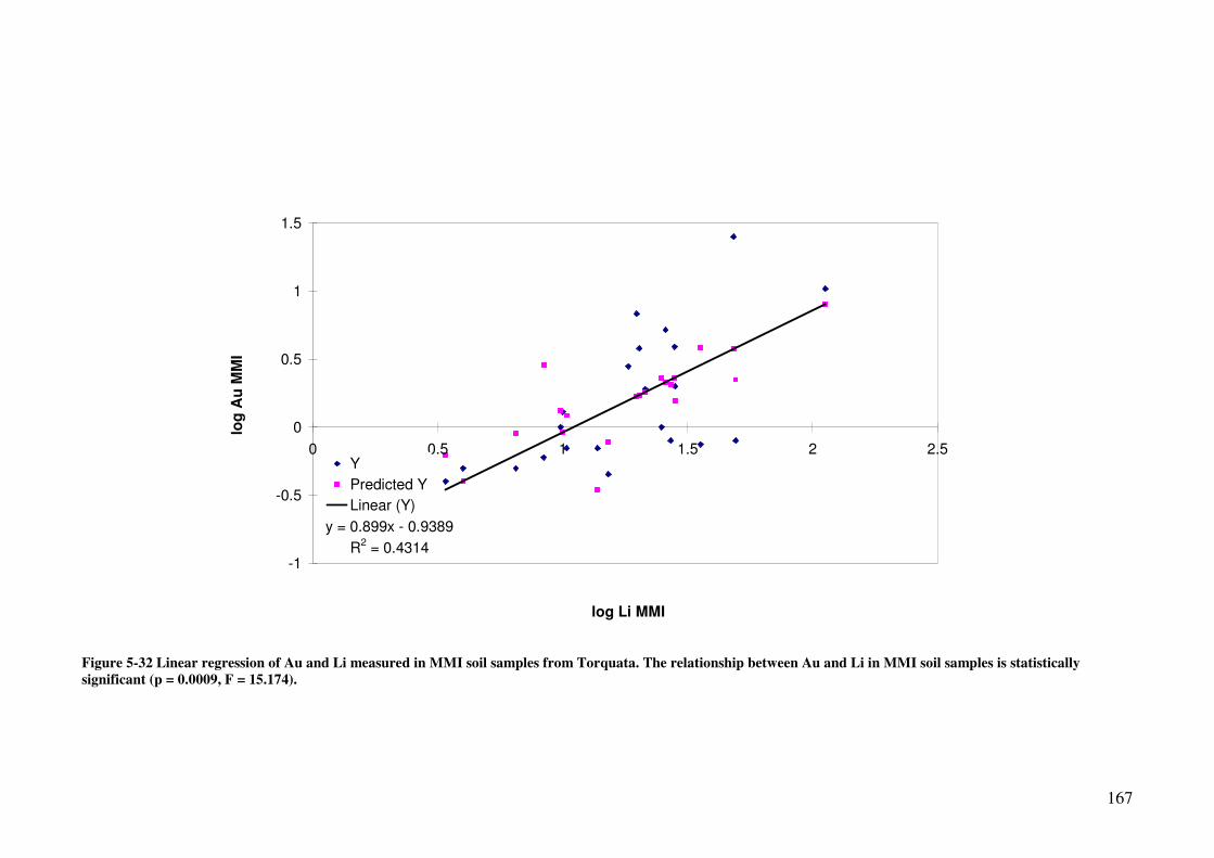
167

y = 0.899x - 0.9389

R2 = 0.4314

-1

-0.5

0

0.5

1

1.5

0 0.5 1 1.5 2 2.5

log Li MMI

log

Au

MM

I

Y

Predicted Y

Linear (Y)

Figure 5-32 Linear regression of Au and Li measured in MMI soil samples from Torquata. The relationship between Au and Li in MMI soil samples is statistically

significant (p = 0.0009, F = 15.174).

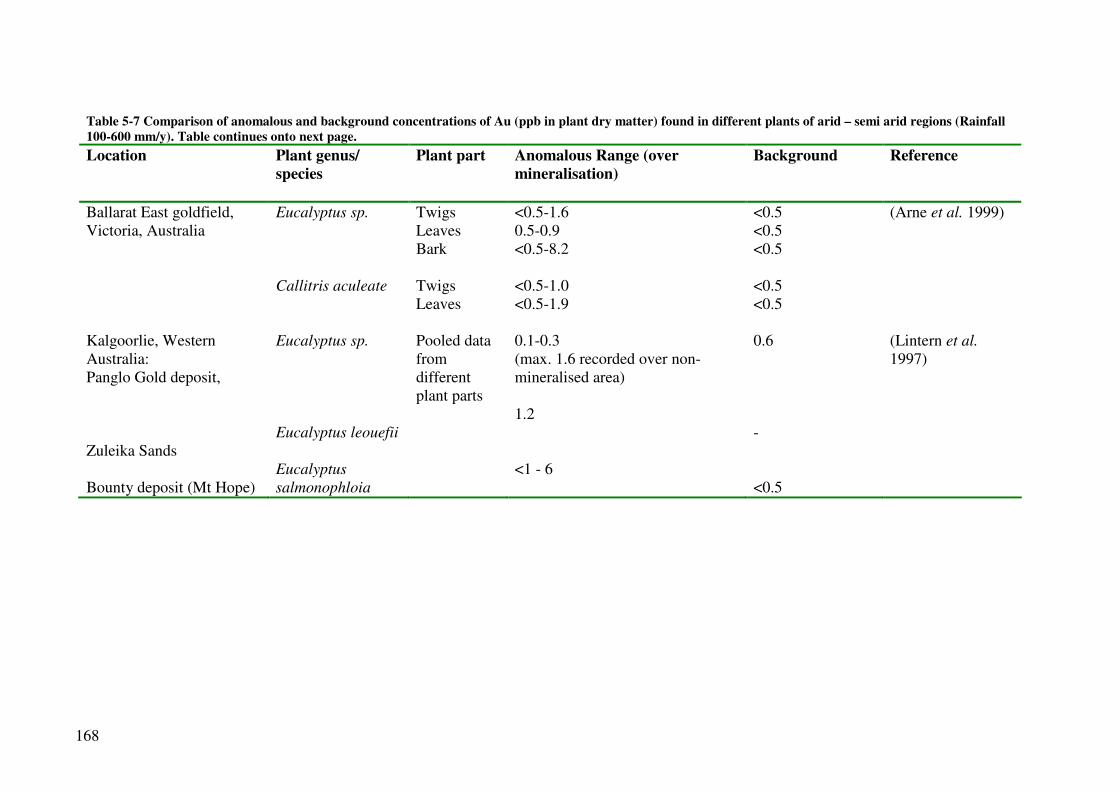
168

Table 5-7 Comparison of anomalous and background concentrations of Au (ppb in plant dry matter) found in different plants of arid – semi arid regions (Rainfall

100-600 mm/y). Table continues onto next page.

Location Plant genus/

species

Plant part Anomalous Range (over

mineralisation)

Background

Reference

Ballarat East goldfield,

Victoria, Australia

Eucalyptus sp.

Callitris aculeate

Twigs

Leaves

Bark

Twigs

Leaves

<0.5-1.6

0.5-0.9

<0.5-8.2

<0.5-1.0

<0.5-1.9

<0.5

<0.5

<0.5

<0.5

<0.5

(Arne et al. 1999)

Kalgoorlie, Western

Australia:

Panglo Gold deposit,

Zuleika Sands

Bounty deposit (Mt Hope)

Eucalyptus sp.

Eucalyptus leouefii

Eucalyptus

salmonophloia

Pooled data

from

different

plant parts

0.1-0.3

(max. 1.6 recorded over non-

mineralised area)

1.2

<1 - 6

0.6

-

<0.5

(Lintern et al.

1997)

169

Table 7 continued.

Location Plant genus/

species

Plant part Anomalous

Range (over

mineralisation)

Background Reference

Barns Gold Prospect, Eyre

Peninsula, South Australia

Eucalyptus incrassata subsp. Incrassate

Melaleuca uncinata

Litter

Leaves

Bark

Litter

Leaves

Bark

1.7

1.1

2.9

0.7

0.4

3.6

0.55

0.3

1.05

0.3

-

0.45

(Lintern

2007)

Berkley Prospect,

Coolgardie, Western

Australia

Eucalyptus sp. Litter

Leaves

Bark

<0.25-3.72

<0.25-3.84

<0.25-5.43

0.61

0.933

0.273

Chapter 3

Torquata Prospect, Western

Australia

Eucalyptus sp. Litter

Leaves

Bark

<0.25-6.20

<0.25-2.49

<0.25-1.56

0.163

0.083

0.453

Chapter 4

1 25

th percentile value from pooled samples across both sampling transects.

170

5.3. Discussion

5.3.1. Source of Au

The data set of drill cores, coupled with the limited biogeochemical data of the surface

environment did not shed any light on the source of the Au at this prospect. High

concentrations of Au (30 – 2900 ppb) occur in at variable depths in the drill cores both

within the transported material and the weathered in situ mudstone/shales. Yet, drilling

deeper past the weathered-partially weathered in situ mudstone/shales into the

Proterozoic sedimentary basement has shown no detectable Au. Drilling indicates that

the Au anomalies in the regolith are restricted to the oxidised zone, regardless of the

type of material (transported overburden/ in situ material) within which the anomalous

Au is found. Au in soils and vegetation corresponded to the high concentrations of Au

found within the surficial calcrete horizon but this is only true for samples from the

northern transect. There is also reasonable correlation between the surface Au signature

in soils and vegetation with anomalous concentrations of Au found deeper in the

regolith at depths as great as 55 m but only in the northern transect. Further, wherever

there is an anomalous concentration of Au in the surface (top 5 m) there is a

correspondingly high concentration of Au deeper in both the transported overburden

and the in situ material (eg. Figure 2 (c) and Figure 3 (b)). The “mottled” pattern of Au

anomalies in the regolith suggests the Au is relatively mobile in the oxidised zone

(above the “saprolite” in Figures 2 (c) and 3 (b)). The strong linear relationship between

the Au and Li measured in the 10-25 cm MMI soil samples further attests to the

mobility of Au in the surface environment. Li is a highly mobile element and its

distribution in soil profiles is highly dependent on the movement of water in the vadose

zone (Kabata-Pendias et al. 1992). Although the source of the Au could not be

determined from this biogeochemical study, clues from the data indicate that the Au

may have hydromorphic origins. Given that Torquata is situated within the Eucla Basin,

an ancient drainage basin, it is possible that Au may have been transported here from

another inland source/diffuse sources on the Yilgarn Plateau and was deposited and

eventually concentrated in the mudstones prior to the deposition of the younger material

on top, either alluvially or by wave motion. The subsequent onset of calcrete formation

may have redistributed the Au into the upper transported sediments. However, the

possibility that the Au may have originated from the transported overburden, which is

also of marine origins, cannot be ruled out either. Further detailed analysis of the soil by

size fractions (e.g. 125 µm-63 µm) may help elucidate the source of the Au at Torquata.

171

For example, in a study of Au dispersion in sediments in Atacama, Chile, Herail et al.

(1999) found high concentrations of Au were associated predominately with the <63 µm

fraction of soil (Herail et al. 1999). In the same vein, analysis of groundwater for Au,

which was detected in some of the drill cores, may also help determine if the Au was

transported through groundwater from another source.

Granted that the source of Au cannot, as yet, be determined by the biogeochemical or

drill core data, the data nevertheless suggest that vegetation plays a part in the formation

of Au within the calcrete horizon. Several authors have already suggested that plants

contribute to the formation of calcrete (Lintern 2007; Mumm et al. 2007). We have

already presented evidence for the mobile nature of Au in the oxidised zone of regolith

at Torquata. Au could eventually work its way into the calcrete structure through co-

precipitation with Ca2+

and carbonate ions (Mumm et al. 2007). Further, the statistically

significant relationship between the Au and Ca found in the leaf samples, and the linear

relationship between the vegetation and soil samples for Au, suggest that these elements

are highly recycled by plants in the surficial environment. Plant senescence returns the

Au to the soil and the seasonal wet dry cycles would then cyclically dissolve the

carbonate and leach the Au deeper into the profile where it is likely to reprecipitate. The

leaching of Au down the regolith during the wet season with precipitation could explain

why high concentrations (>100 ppb) of Au were found deeper within certain parts of the

regolith. Sequential extraction of the upper soil horizons, for example by extractants

targeting the organic pool of elements as well as that targeting the carbonate or

exchangeable pool (Hall et al. 1996) may help determine if vegetation were indeed

involved in the accumulation of the Au in the near surface calcrete (also refer to Chapter

3).

Due to the observations that i) the source of the Au is unknown and ii) the presence of

large concentrations of Au in the surficial environment (5 m of the soil), we have no

conclusive proof that the deep uptake of Au by vegetation has taken place in the past or

is taking place. It is likely the current concentration of Au in the plant tissues may just

be the Au being recycled surficially. Similarly, because of the presence of the large

near-surface Au anomaly, we could not examine the effect of transported overburden

depth on the concentrations of Au in the surficial environment.

172

5.3.2. Biogeochemical accumulation of elements in soil and vegetation

Both the soils and vegetation at Torquata show elevated concentrations of Au relative to

the 25th

percentile (background) concentrations, particularly in the northern transect,

which corresponded with the locations where anomalous concentrations of Au in the

regolith are found. It is striking that both vegetation and soil analyses show markedly

different results between the two sampling transects. Overall, the soil and vegetation

response was significantly larger in the northern transect (6511 200N) compared with

the southern transect (6510 440N). The samples from the northern transect also showed

excellent correlation with the Au anomalies found in the drill cores. In stark contrast,

the vegetation samples from the southern transect showed no correlation with the soil

samples and both the vegetation and soil samples showed little correlation with the drill

core samples for Au. The differences between the data from the northern transect and

the southern transect were particularly evident from the soil samples, which show low

concentrations of Au along the southern transect (maximum concentration measured at

574 594E, 6510 440N was 4 ppb), compared with >200 ppb measured in some soil

samples from the northern transect. The different responses obtained from the

vegetation and soils from the two transects, highlights the inherent difficulties in

applying the biogeochemical method in exploration. Although we have kept the

vegetation sampling consistent (i.e. the consistent plant parts; standard sampling height

(~1.5 m) with the methodology from the literature (Dunn et al. 1995; Lintern et al.

1997; Anand et al. 2007) it is possible that the plants along the southern transect may

not be taking up water and nutrients from the same depth as the drill core where there is

an anomalous accumulation of Au. This may be because the plants along the southern

transect were completely burnt and the samples collected were of recent regrowth

(plants approximately 0.5m high, sampled approximately 3 months after the fire). There

may perhaps be a significant difference in the ability of young plants and that of mature

trees to take up and store ore related elements. The fire would also have caused

significant loss to the litter layer (the litter layer was observed to be sparser here) and

could thus have resulted in lower litter response ratios.

Data from Torquata also shows that the vegetation and soils are not only enriched in Au

relative to the background but also in rare earth elements, which were not determined in

the drill core samples. The Eucla Basin in Australia is known for its placer Au and

heavy mineral sands deposits (commonly enriched in rare earth elements) (Hou et al.

2005; Government of South Australia 2007), so it is perhaps not surprising that we have

173

found an accumulation of rare earth elements in both soils and vegetation at Torquata.

As it is likely that the Au mineralization at the Torquata site may have been brought

about by marine depositional fluxes or terrigenous fluxes from inland rivers, it is

possible that the density/wave sorting in the old marine environment could have brought

about co-deposition of the Au with the REE and hence the anomalous concentrations of

REE that were detected in the soils

Comparison of the Au concentrations in our vegetation samples with those from the

literature has shown some similarity with other Australian data. Table 5-7 shows the

concentration range for Au in different plant species from Australia. In general, the

concentration ranges in leaves and litter over mineralisation (irrespective of the type of

deposit and the species) for the genus Eucalyptus ranged from 0.4 ppb – 8 ppb in

Australian studies within which our vegetation samples from Torquata and Berkley fall.

The higher anomaly contrast observed for leaf samples compared with litter samples is

in contrast to other findings (Dunn et al. 1986; Lintern et al. 1997; Anand et al. 2007).

The differences between our study and other studies is most likely due to the effects of

the fire, where possibly much of the litter layer has been lost (particularly along the

southern transect). In addition, similar concentrations in the partial extraction of the 0-

4 cm (representing the organic soil horizon) soil samples (MMI analysis) and the 10-

25cm soil samples were obtained for most elements except Th. Thorium is significantly

more enriched in the 0-4 cm soil depth than the 10-25 cm depth. This seems contrary to

observations from the literature where Th is reportedly taken up by plants to a lesser

extent and less mobile than other REE in plants because of adsorption on cell wall

material (McClellan et al. 2003). Dunn et al. (1986) also seem to suggest the same

exclusion of Th and U from plant material, although our data suggest no difference in U

concentrations between the two different soil depths. Further, results from the aqua

regia digests showed significant difference between the 0-4 cm and 10-25 cm soil

samples for all elements measured except Pb. Lead is less mobile than many other trace

elements in the environment, and this may explain the Pb concentration difference

between the two soil depths. Our data for the 0-4 cm aqua regia digests agree with that

of Anand et al. (2007) where soil from 0-4 cm is more enriched in trace elements than

the mineral horizon (10-20 cm).

174

5.4. Conclusions

We were unable to determine the source of the large surficial Au anomaly in calcrete. It

is possible that, given the siting of Torquata within the Eucla Basin, a Cainozoic

drainage basin, that the source of the calcrete Au may itself be the remnant

hydromorphic dispersion trail and/or detrital Au transported from another unknown

inland source of Au. However, the strong correlations between Au and Ca in both the

leaf and litter samples and the 10-25cm soil MMI samples suggests the vegetation may

have contributed to the formation of the Au in calcrete. High concentrations of Au were

found in both vegetation matter and the surface soils. Overall, we found that the leaf

samples gave better anomaly contrast to the litter samples. However, we did not have

enough sample mass from either the bark or the twigs to truly test which plant organ

gave the best response. Further detailed analysis of the size fractions of soils for Au

(e.g. <63 µm) may help elucidate the source of Au. Analysis of groundwater for Au

may also help determine if the Au was transported through groundwater from another

source.

175

CHAPTER SIX

Quantitative modelling of trace element accumulation in surficial soils

by plant uptake from depth in the regolith: Application to mineral

exploration under transported cover

6. Introduction

Given the declining rate of mineral discovery in Australia, the rewards are relatively

low compared with the risk involved in making the discovery (Centre for Exploration

Targetting 2007). As economic demands grow, future discoveries of metal deposits will

ultimately lie in terrains covered by transported overburden where sampling of surficial

materials (soil and lag) has been shown to be less effective in delineating mineralisation

(Butt et al. 2000; Anand et al. 2007). Exploration for mineral deposits under transported

cover, however, remains a major challenge to the mining industry (Anand et al. 2007;

Lintern 2007) and requires a sound understanding of formative processes of

geochemical signatures to determine the best exploration strategy to implement. Thus,

there is great need for the development of predictive models to improve the current

understanding of how geochemical footprints of mineralisation form, with the ultimate

goal of a better selection of exploration strategies, particularly in the area of greenfields

exploration.

With the push to expand exploration into covered terranes, the use of plants as a

prospecting tool is currently a hot topic in the exploration community. Field evidence

has shown soils developed from recently deposited overburden sometimes develop the

distinct geochemical signature of the buried mineral deposit (Cameron et al. 2004;

Radford et al. 1999; Scott et al. 1999) (Also see Chapter 2). Several authors have

proposed that deep nutrient and water uptake by deep rooted plants, under the right

circumstances, may be key to the development of soil geochemical anomalies in

recently deposited overburden (Anand et al. 2007; Lintern 2007). It is well known that

vegetation can affect trace element distribution in the regolith by physically and

chemically altering their immediate environment (Dakora et al. 2002; Stretch et al.

2002; Jobbagy et al. 2004). Deep rooted plants can effectively redistribute elements

from a large volume of regolith into the surficial environment (Dunn 1981; Jobbagy et

al. 2004). Under a sufficiently long time span (>106 yrs), the uptake of ions by

vegetation at depth in the regolith could lead to the concentration of trace elements in

176

the surface soil in semi-arid/arid environments. However, this deep plant uptake flux

remains, as yet, unquantifiable.

Due to the difficulty in directly measuring deep plant uptake fluxes, a biogeochemical

mass balance should provide a close approximation. The rates obtained from the mass

balance could then be used as proxies for the development of rate expressions for the

soil-plant-mineralisation system. These expressions could be used to simulate the

formation of biogeochemical footprints of mineralisation over time. At the same time,

key fluxes influencing the size and development of biogeochemical signatures can be

identified.

In this chapter, rate constants are derived for the development of a differential equation

model. Data sourced from both the literature (see Chapter 2) and from our own analyses

of field samples were used as inputs into the mass balance. The rate expressions for a

deep botanical element uptake flux are presented for the first time in this work. A

simple first order ordinary differential equation (ODE) model was then used to: i)

simulate the formation of soil anomalies through plant uptake of ore elements from

depth; and ii) test the conditions under which a biogeochemical signature may be

produced in the surficial environment.

6.1. Background

Understanding the formative processes of biogeochemical signatures in plant and soils

is important in mineral exploration, particularly if biogeochemistry is to be used as an

exploration tool. Aside from problems with standardising the biogeochemical method,

soil anomalies may not always be found despite the presence of a vegetation anomaly,

particularly in areas of transported cover (shown by both studies in the literature (Cohen

et al. 1999) and from our own case studies from Berkley (Chapter 4) and Torquata

(Chapter 5)). Why is there sometimes no soil response? A simple biogeochemical model

may help to explain these observations.

Geochemical mass balances are considered the most robust technique for determining

the rates of element movement in the surficial environment (Velbel et al. 2007). In the

absence of direct experimental measurement of plant uptake rates from deep in the

regolith, a geochemical mass balance may provide an estimate. To our knowledge, only

177

a handful of studies currently exist on geochemical mass balances that specifically

account for a botanical uptake term (Velbel 1986; Taylor et al. 1991; Lintern 2007).

Vegetation not only provides feedback to important processes like weathering (Dakora

et al. 2002; Stretch et al. 2002) but also in redistributing elements into the surficial

environment (Dunn et al. 1995; Jobbagy et al. 2004). Thus, accounting for the

vegetation reservoir and its associated fluxes is critical in geochemical mass balances.

Lintern (2007), using present day measurements of concentrations in the vegetation, net

primary productivity and total mass of Au in the regolith profile (for a sand dune),

arrived at an age estimate for the deposition of Au in the surficial environment solely by

deep uplift of Au by vegetation (ca. 10 000 y for a dune height of 8 m). This age

estimate is much smaller than the age of the dune (ca. 26 000 y), providing sufficient

time for surface recycling to occur. Surface recycling would indeed be expected to

dominate over the rate of deep uplift since it has been noted by several workers that

nutrient uptake from depth is significantly less than uptake at the surface (Taylor et al.

1991; Poszwa et al. 2002). Taylor and Velbel (1991) estimate surface recycling rates to

vary between 85 – 90% of total nutrient uptake by vegetation in ecosystems. Provided

that plant nutrient uptake takes place at a greater depth than plant return in the soil

profile, however, there is grounds for net uplift of elements to occur (Jobbagy et al.

2004). Hence even if only 1% of nutrient uptake is contributed by deep roots over a

period of 106 -10

7 y, significant concentrations of elements could be redistributed into

the surface environment. In water limited ecosystems, the contribution of deep roots to

nutrient uptake is expected to be more significant (Poszwa et al. 2002).

The net uptake flux of elements will also be counterbalanced by the loss fluxes of

erosion (Jobbagy 2004) and leaching (Freyssinet 1997). The model in Lintern (2007)

did not include an erosion term. The initial mass balance calculations from Chapter 2

showed that erosion is a key variable in influencing the development of soil anomalies.

Other similar quantitative models (e.g. pedogenesis) have also shown that erosion is an

important variable keeping the net inflow fluxes in check (Minasny et al. 1999;

Minasny et al. 2001). Hence, over ecological time scales, exclusion of an erosion term

could lead to an over estimation in the amount of element accumulation in the soil. The

other mode of loss through the soil system is through leaching. In semi-arid - arid

environments however, loss from the soil through leaching is expected to be minimal

(typically, net downward water movement is <50mm/y).

178

Biogeochemical anomalies can thus be produced as a result of net accumulative fluxes

through plant uptake operating in the system. Since accumulative and loss fluxes exist

in a sort of disequilibrium, we hypothesised earlier that soil anomalies may only be

transient features as all fluxes shift towards a steady-state. Subsequently, any vegetation

anomaly will also be a transient feature as it too will eventually reach equilibrium with

the soil, as the source gets depleted.

In order to enable evaluation of the long-term impact of processes such as deep nutrient

uptake on the soil and vegetation, differential equation modelling is required. There are

currently no rate expressions that predict the redistribution of elements by biota from a

concentrated source into other reservoirs. Having rate expressions allows us to simplify

several biogeochemical processes into an elegant mathematical expression. The

feasibility of a biotic mechanism for the accumulation of ore-elements in the soil and

vegetation may then be evaluated. The main advantage of this approach is that a simple

cost-effective tool can be developed to aid the decision making process in selecting an

appropriate exploration strategy. Such a model would also be informative because it is

mechanistic and quantifies “real” processes operating in ecosystems.

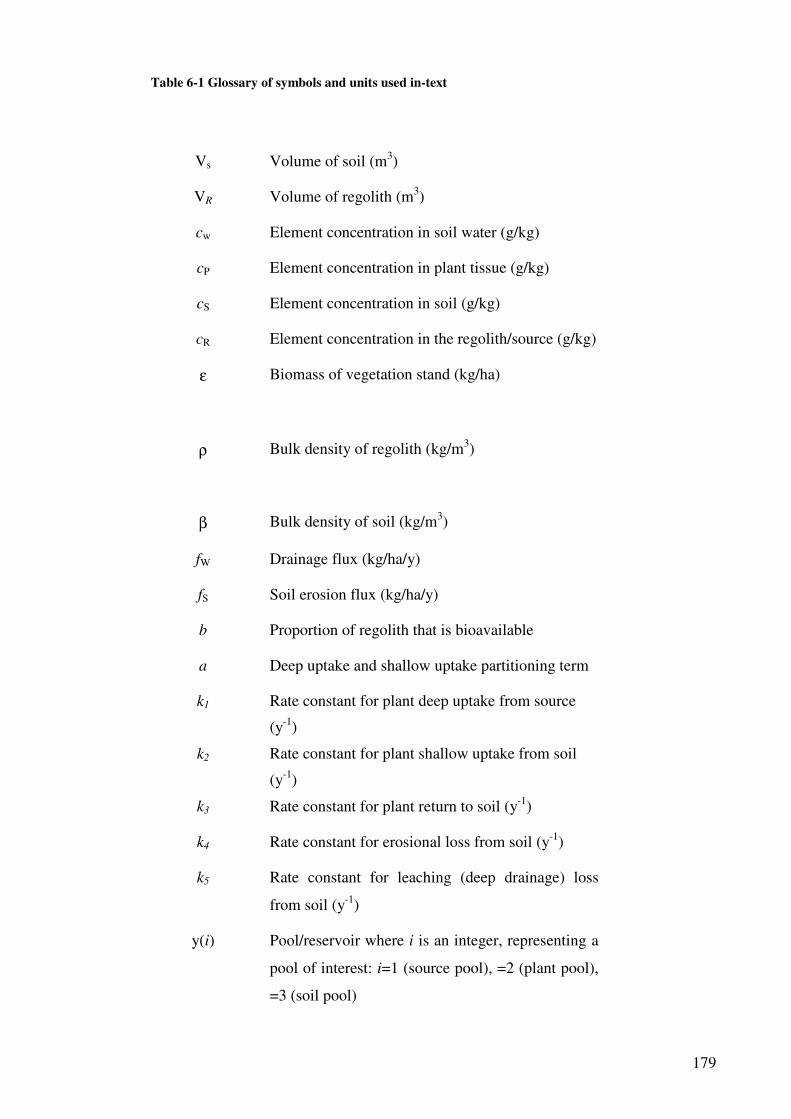
179

Table 6-1 Glossary of symbols and units used in-text

Vs

Volume of soil (m3)

VR Volume of regolith (m3)

cw Element concentration in soil water (g/kg)

cP Element concentration in plant tissue (g/kg)

cS Element concentration in soil (g/kg)

cR Element concentration in the regolith/source (g/kg)

ε

Biomass of vegetation stand (kg/ha)

ρ

Bulk density of regolith (kg/m3)

β Bulk density of soil (kg/m3)

fW Drainage flux (kg/ha/y)

fS Soil erosion flux (kg/ha/y)

b Proportion of regolith that is bioavailable

a Deep uptake and shallow uptake partitioning term

k1 Rate constant for plant deep uptake from source

(y-1

)

k2 Rate constant for plant shallow uptake from soil

(y-1

)

k3 Rate constant for plant return to soil (y-1

)

k4 Rate constant for erosional loss from soil (y-1

)

k5 Rate constant for leaching (deep drainage) loss

from soil (y-1

)

y(i) Pool/reservoir where i is an integer, representing a

pool of interest: i=1 (source pool), =2 (plant pool),

=3 (soil pool)

180


Mass balances were carried out in Microsoft Excel®. Scilab© (Version 4.1) (INRIA,

ENPC) was used as a platform for all our modelling simulations. Data input for our

model was obtained from various sources in the literature (see Chapter 2) as well as

from our own case studies (see Chapters 3 and 4).

6.2.1. General assumptions and simplifications

This section details the general assumptions and simplifications used. The first implicit

assumption is that the simulations are carried out under conditions typical of semi-

arid/arid ecosystems. Secondly, the net primary productivity of the vegetation stand (as

well as the biomass) is assumed to be constant over time. We have already argued

elsewhere (Chapter 2) that biotic uplift of elements is the most likely mechanism for

vertical transport to dominate over other physical mechanisms. Further, the models

simulate two-dimensional, vertical transport through the regolith over time. It is

assumed that plants root to within reach of the source and deposit metals evenly over

the soil anomaly. Additionally, it is known that elements reside in the litter reservoir

prior to decay and return to the soil (Attiwill et al. 1987). However, as the rate of plant

turnover is assumed to be immediate relative to the timescale of the simulations, the

models therefore, do not account for any residence time in the litter reservoir. After

Heimsath et al. (1997) and Buss et al. (2005), the total mass of the regolith (including

soil) is also assumed to be in steady state between soil production and loss through

weathering and erosion over time. Finally, any erosional or leaching loss is also

assumed to occur evenly over the extent of the soil anomaly.

6.2.2. Differential equations

All rate equations are assumed to fit a first order ordinary differential equation, i.e. the

rates of change of the reservoirs are dependant on one variable, the initial reservoir size

(y0). The equations are set up as follows for the reservoirs:

(A) Source y(1) (Source: represents a buried ore body/ accumulation of ore elements in

deeper regolith)

)1()1(

1 ykdt

dy⋅−= Equation 6-1

181

Where y(1) is the initial concentration of element in the source reservoir. The

concentrations used in the simulation were obtained from measurements of

anomalous concentrations of elements in the regolith. k1 is the rate of deep uptake

from the source reservoir. k1 is not a true rate constant but is dependant upon NPP,

biomass and the regolith (source) concentration. Studies of deep nutrient uptake in

semi-arid ecosystems seem to indicate that 50-90% of total nutrient uptake by plants

comes from surficial recycling (Taylor et al. 1991). Furthermore, Schenk and

Jackson (2005) have also shown that approximately 5% of the total root biomass of

most trees comprises of deep roots (>4 m length). Therefore, the deep uptake rate

can be assumed to be approximately 2-5% of the shallow uptake rate. Hence, k1 can

thus be derived:

k1= a · (NPP · cR )/ ε Equation 6-2

Where a is the partitioning ratio between the deep (k1) and the shallow (k2) element

uptake flux and ranges between 0.02-0.05. NPP is the net primary productivity; cR

is the concentration of the source and ε is the vegetation biomass.

(B) Vegetation y(2)

y(2)*k - y(3)*k y(1)*k)2(

321 +=

dt

dy Equation 6-3

Where y(2) is the initial concentration of the target element measured in vegetation,

the background average plant concentration. k1 is the rate of deep uptake from the

source reservoir. y(3) is the initial concentration of the soil reservoir. k2 is the

shallow uptake rate of the target element from the soil reservoir. k3 is the rate of

return of the target element to the soil reservoir. It is assumed that both the shallow

uptake rate (k2) and the rate of plant return (k3) are correlated to the net carbon

accumulation and loss from the vegetation reservoir, i.e. the net primary

productivity (NPP) of the ecosystem (Attiwill et al. 1987)(Refer to Chapter 2 for list

of NPP values used in the simulations). For simplicity, we assumed that the net

plant return, k3, is the sum of the total element uptake therefore, whatever is gained

by the plant reservoir is returned to the soil. In a second simulation, the total

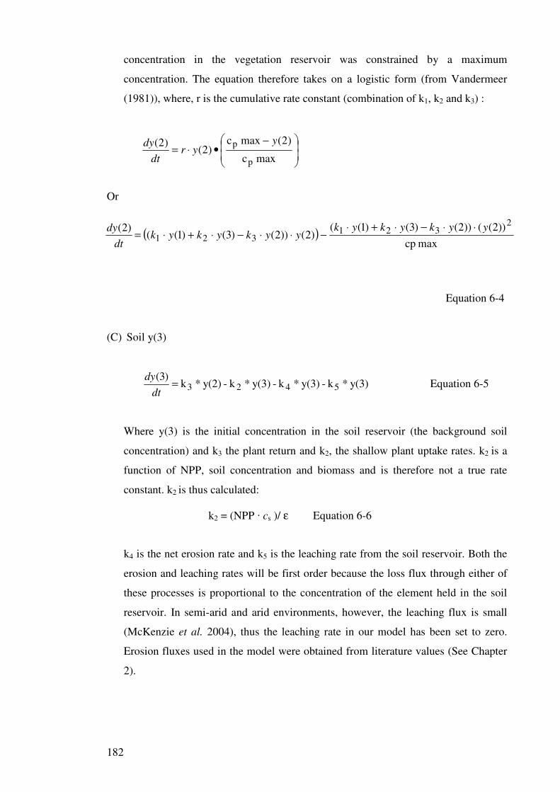
182

concentration in the vegetation reservoir was constrained by a maximum

concentration. The equation therefore takes on a logistic form (from Vandermeer

(1981)), where, r is the cumulative rate constant (combination of k1, k2 and k3) :

−

•⋅=

max c

)2(max c)2(

)2(

p

p yyr

dt

dy

Or

( )

max cp

))2(())2()3()1(()2())2()3()1((

)2(2

321321

yykykykyykykyk

dt

dy ⋅⋅−⋅+⋅

−⋅⋅−⋅+⋅=

Equation 6-4

(C) Soil y(3)

y(3)*k - y(3)*k - y(3)*k- y(2)*k)3(

5423=

dt

dy Equation 6-5

Where y(3) is the initial concentration in the soil reservoir (the background soil

concentration) and k3 the plant return and k2, the shallow plant uptake rates. k2 is a

function of NPP, soil concentration and biomass and is therefore not a true rate

constant. k2 is thus calculated:

k2 = (NPP · cs )/ ε Equation 6-6

k4 is the net erosion rate and k5 is the leaching rate from the soil reservoir. Both the

erosion and leaching rates will be first order because the loss flux through either of

these processes is proportional to the concentration of the element held in the soil

reservoir. In semi-arid and arid environments, however, the leaching flux is small

(McKenzie et al. 2004), thus the leaching rate in our model has been set to zero.

Erosion fluxes used in the model were obtained from literature values (See Chapter

2).

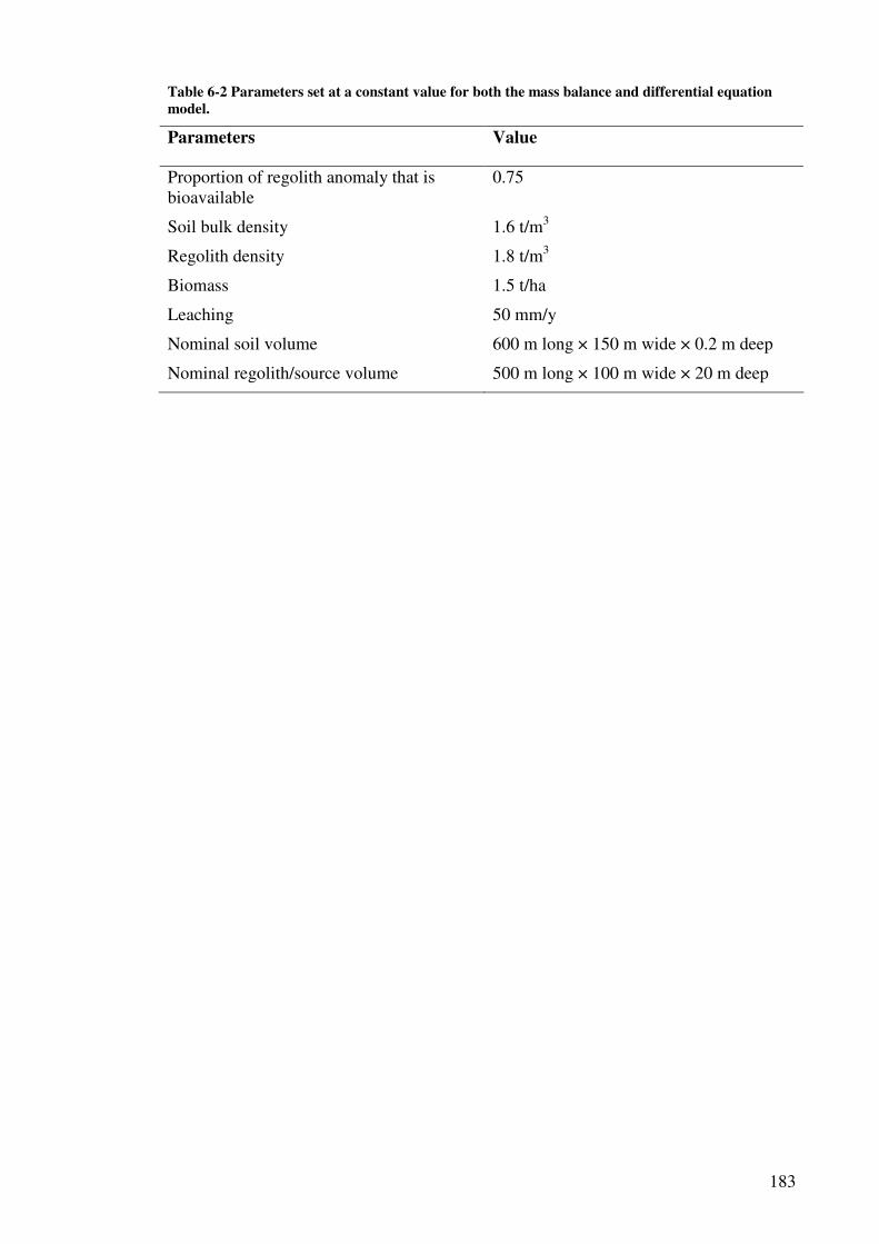
183

Table 6-2 Parameters set at a constant value for both the mass balance and differential equation

model.

Parameters Value

Proportion of regolith anomaly that is

bioavailable

0.75

Soil bulk density 1.6 t/m3

Regolith density 1.8 t/m3

Biomass 1.5 t/ha

Leaching 50 mm/y

Nominal soil volume 600 m long × 150 m wide × 0.2 m deep

Nominal regolith/source volume 500 m long × 100 m wide × 20 m deep

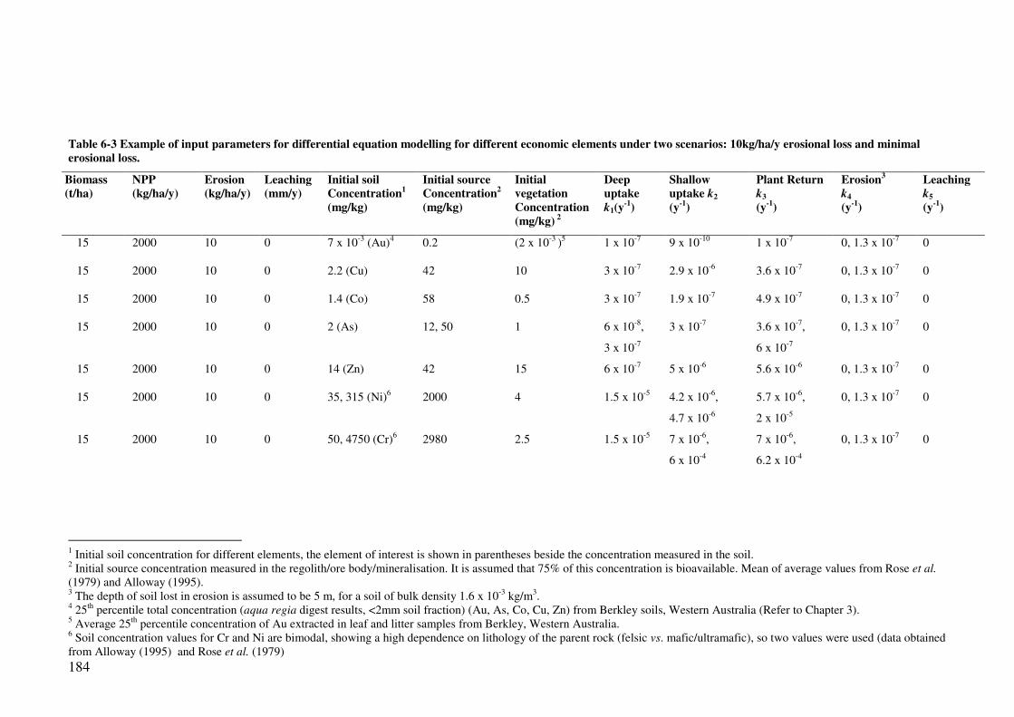
184

Table 6-3 Example of input parameters for differential equation modelling for different economic elements under two scenarios: 10kg/ha/y erosional loss and minimal

erosional loss.

Biomass

(t/ha)

NPP

(kg/ha/y)

Erosion

(kg/ha/y)

Leaching

(mm/y)

Initial soil

Concentration1

(mg/kg)

Initial source

Concentration2

(mg/kg)

Initial

vegetation

Concentration

(mg/kg) 2

Deep

uptake

k1(y-1

)

Shallow

uptake k2

(y-1

)

Plant Return

k3

(y-1

)

Erosion3

k4

(y-1

)

Leaching

k5

(y-1

)

15 2000 10 0 7 x 10-3

(Au)4 0.2 (2 x 10

-3 )5 1 x 10

-7 9 x 10

-10 1 x 10

-7 0, 1.3 x 10

-7 0

15 2000 10 0 2.2 (Cu) 42 10 3 x 10-7

2.9 x 10-6

3.6 x 10-7

0, 1.3 x 10-7

0

15 2000 10 0 1.4 (Co) 58 0.5 3 x 10-7

1.9 x 10-7

4.9 x 10-7

0, 1.3 x 10-7

0

15 2000 10 0 2 (As) 12, 50 1 6 x 10-8

,

3 x 10-7

3 x 10-7

3.6 x 10-7

,

6 x 10-7

0, 1.3 x 10-7

0

15 2000 10 0 14 (Zn) 42 15 6 x 10-7

5 x 10-6

5.6 x 10-6

0, 1.3 x 10-7

0

15 2000 10 0 35, 315 (Ni)6 2000 4 1.5 x 10

-5 4.2 x 10

-6,

4.7 x 10-6

5.7 x 10-6

,

2 x 10-5

0, 1.3 x 10-7

0

15 2000 10 0 50, 4750 (Cr)6 2980 2.5 1.5 x 10

-5 7 x 10

-6,

6 x 10-4

7 x 10-6

,

6.2 x 10-4

0, 1.3 x 10-7

0

1 Initial soil concentration for different elements, the element of interest is shown in parentheses beside the concentration measured in the soil.

2 Initial source concentration measured in the regolith/ore body/mineralisation. It is assumed that 75% of this concentration is bioavailable. Mean of average values from Rose et al.

(1979) and Alloway (1995). 3 The depth of soil lost in erosion is assumed to be 5 m, for a soil of bulk density 1.6 x 10

-3 kg/m

3.

4 25

th percentile total concentration (aqua regia digest results, <2mm soil fraction) (Au, As, Co, Cu, Zn) from Berkley soils, Western Australia (Refer to Chapter 3).

5 Average 25

th percentile concentration of Au extracted in leaf and litter samples from Berkley, Western Australia.

6 Soil concentration values for Cr and Ni are bimodal, showing a high dependence on lithology of the parent rock (felsic vs. mafic/ultramafic), so two values were used (data obtained

from Alloway (1995) and Rose et al. (1979)

185

6.3. Results and Discussion

6.3.1. First order differential equation modelling

Numerical modelling with first order differential equations for Au accumulation in soils

shows that at just 0.2 ppm regolith concentration of Au, soil anomalies will not form by

means of plant uptake (Figure 6-1 (a)). Plants are the first to respond to the source

before the soil. Given the same set of parameters: NPP = 2000 kg/ha/y;

erosion = 0 kg/ha/y, the regolith concentration of Au needs to be at least 20 ppm for

significant (soil response >5 times background) to occur. However, the results do not

match field evidence at Berkley where as much as 200 ppb Au was measured in the

surface soils despite a maximum measured concentration in regolith or host rocks of

0.2 ppm-1 ppm. The Au simulation also does not agree with the mass balance in

Chapter 2 or with the literature, where sometimes significant accumulation in the soil

and vegetation reservoirs occurs over <1 ppm of source Au. Two significant

implications arise from the modelling results for Au. Firstly, even under the given

conditions of a relatively productive ecosystem (2000 kg/ha/y) with no erosion, it is

highly unlikely that a soil anomaly for Au will form through biotic uplift alone because

the rate constants for net uptake are too small. A corollary of the simulation outcome is

that there is a minimum starting concentration for the source pool for Au (>10 ppm).

Conversely, this result could also imply that a significant soil response for Au through

biotic uplift may take upwards of 100 My to form.

Sensitivity analyses on the parameters that would lead to the formation of

biogeochemical anomalies were carried out using typical values for Cu concentration in

biogeochemical system components. Firstly, the effects of describing the vegetation

response using a logistic curve on the corresponding soil response was examined

(Figure 6-1). If there is no erosional loss from the soil, the concentration in the

vegetation reservoir remains constant while the concentration in the soil increases as

deep uptake continues to cause net accumulation in the soil. At a small erosion rate of

10 kg/ha/y, the loss from the soil shows a peak in accumulation and eventual decline in

the soil reservoir. The vegetation concentration also shows a gradual decline from a

maximum concentration (the constrained concentration) due to the feedback loop into

the vegetation reservoir as the shallow uptake flux from the soil reduces (Figure 6-2

(a)). Increasing the erosion rate to 25 kg/ha/y produces a sharper peak in both the soil

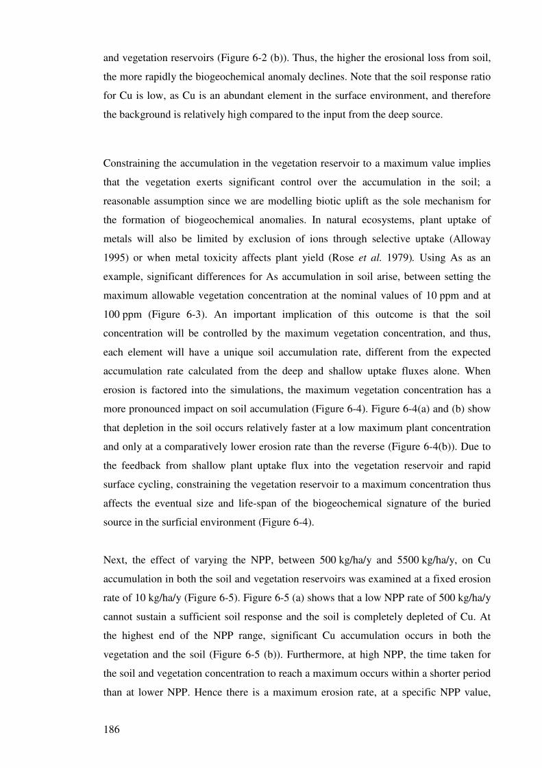
186

and vegetation reservoirs (Figure 6-2 (b)). Thus, the higher the erosional loss from soil,

the more rapidly the biogeochemical anomaly declines. Note that the soil response ratio

for Cu is low, as Cu is an abundant element in the surface environment, and therefore

the background is relatively high compared to the input from the deep source.

Constraining the accumulation in the vegetation reservoir to a maximum value implies

that the vegetation exerts significant control over the accumulation in the soil; a

reasonable assumption since we are modelling biotic uplift as the sole mechanism for

the formation of biogeochemical anomalies. In natural ecosystems, plant uptake of

metals will also be limited by exclusion of ions through selective uptake (Alloway

1995) or when metal toxicity affects plant yield (Rose et al. 1979). Using As as an

example, significant differences for As accumulation in soil arise, between setting the

maximum allowable vegetation concentration at the nominal values of 10 ppm and at

100 ppm (Figure 6-3). An important implication of this outcome is that the soil

concentration will be controlled by the maximum vegetation concentration, and thus,

each element will have a unique soil accumulation rate, different from the expected

accumulation rate calculated from the deep and shallow uptake fluxes alone. When

erosion is factored into the simulations, the maximum vegetation concentration has a

more pronounced impact on soil accumulation (Figure 6-4). Figure 6-4(a) and (b) show

that depletion in the soil occurs relatively faster at a low maximum plant concentration

and only at a comparatively lower erosion rate than the reverse (Figure 6-4(b)). Due to

the feedback from shallow plant uptake flux into the vegetation reservoir and rapid

surface cycling, constraining the vegetation reservoir to a maximum concentration thus

affects the eventual size and life-span of the biogeochemical signature of the buried

source in the surficial environment (Figure 6-4).

Next, the effect of varying the NPP, between 500 kg/ha/y and 5500 kg/ha/y, on Cu

accumulation in both the soil and vegetation reservoirs was examined at a fixed erosion

rate of 10 kg/ha/y (Figure 6-5). Figure 6-5 (a) shows that a low NPP rate of 500 kg/ha/y

cannot sustain a sufficient soil response and the soil is completely depleted of Cu. At

the highest end of the NPP range, significant Cu accumulation occurs in both the

vegetation and the soil (Figure 6-5 (b)). Furthermore, at high NPP, the time taken for

the soil and vegetation concentration to reach a maximum occurs within a shorter period

than at lower NPP. Hence there is a maximum erosion rate, at a specific NPP value,

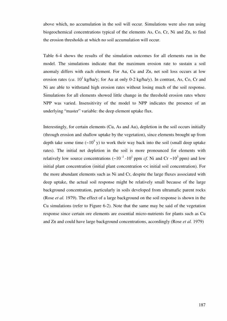
187

above which, no accumulation in the soil will occur. Simulations were also run using

biogeochemical concentrations typical of the elements As, Co, Cr, Ni and Zn, to find

the erosion thresholds at which no soil accumulation will occur.

Table 6-4 shows the results of the simulation outcomes for all elements run in the

model. The simulations indicate that the maximum erosion rate to sustain a soil

anomaly differs with each element. For Au, Cu and Zn, net soil loss occurs at low

erosion rates (ca. 101 kg/ha/y; for Au at only 0-2 kg/ha/y). In contrast, As, Co, Cr and

Ni are able to withstand high erosion rates without losing much of the soil response.

Simulations for all elements showed little change in the threshold erosion rates where

NPP was varied. Insensitivity of the model to NPP indicates the presence of an

underlying “master” variable: the deep element uptake flux.

Interestingly, for certain elements (Cu, As and Au), depletion in the soil occurs initially

(through erosion and shallow uptake by the vegetation), since elements brought up from

depth take some time (~105 y) to work their way back into the soil (small deep uptake

rates). The initial net depletion in the soil is more pronounced for elements with

relatively low source concentrations (~10 -1

-101 ppm cf. Ni and Cr ~10

3 ppm) and low

initial plant concentration (initial plant concentration << initial soil concentration). For

the more abundant elements such as Ni and Cr, despite the large fluxes associated with

deep uptake, the actual soil response might be relatively small because of the large

background concentration, particularly in soils developed from ultramafic parent rocks

(Rose et al. 1979). The effect of a large background on the soil response is shown in the

Cu simulations (refer to Figure 6-2). Note that the same may be said of the vegetation

response since certain ore elements are essential micro-nutrients for plants such as Cu

and Zn and could have large background concentrations, accordingly (Rose et al. 1979)

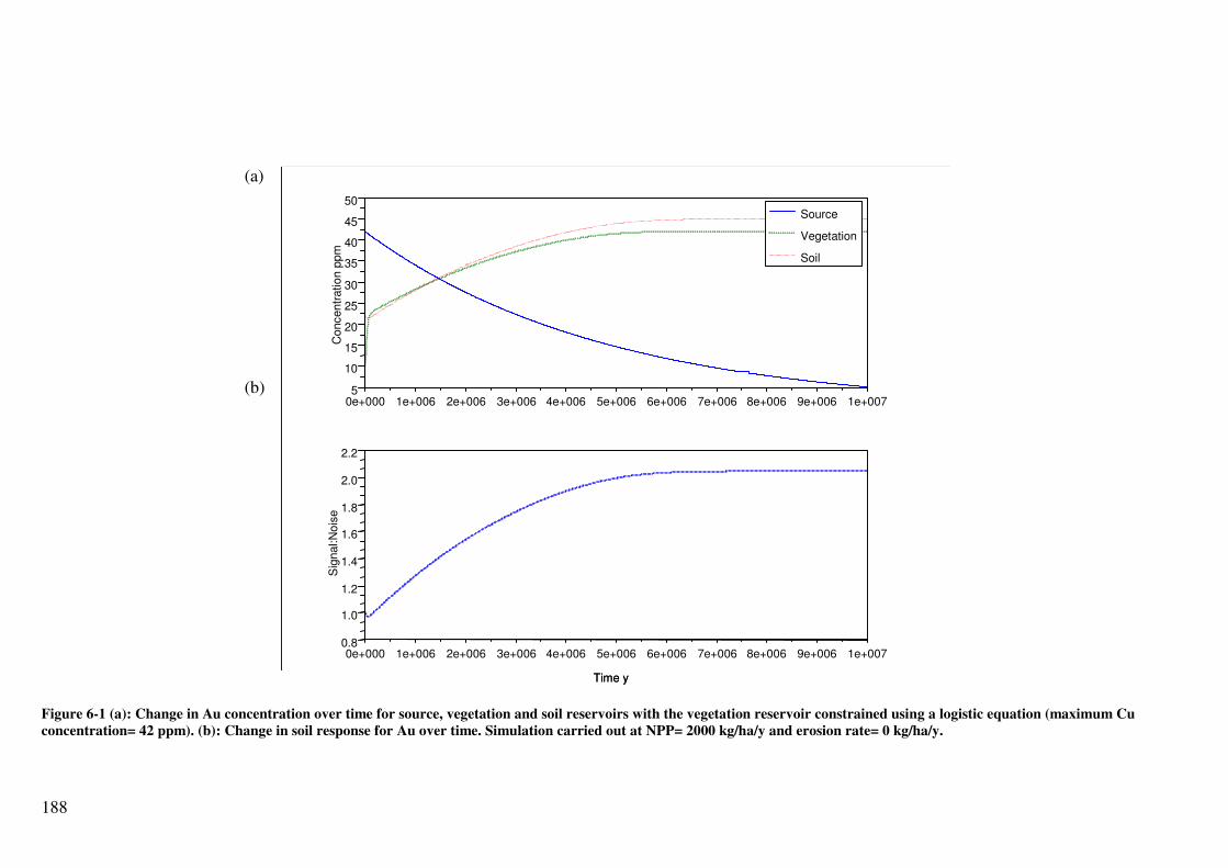
188

(a)

(b) 0e+000 1e+006 2e+006 3e+006 4e+006 5e+006 6e+006 7e+006 8e+006 9e+006 1e+0075

10

15

20

25

30

35

40

45

50

Concentr

atio

n p

pm

Source

Vegetation

Soil

0e+000 1e+006 2e+006 3e+006 4e+006 5e+006 6e+006 7e+006 8e+006 9e+006 1e+0070.8

1.0

1.2

1.4

1.6

1.8

2.0

2.2

Time y

Sig

nal:N

ois

e

0e+000 1e+006 2e+006 3e+006 4e+006 5e+006 6e+006 7e+006 8e+006 9e+006 1e+0075

10

15

20

25

30

35

40

45

50

Concentr

atio

n p

pm

Source

Vegetation

Soil

0e+000 1e+006 2e+006 3e+006 4e+006 5e+006 6e+006 7e+006 8e+006 9e+006 1e+0070.8

1.0

1.2

1.4

1.6

1.8

2.0

2.2

Time y

Sig

nal:N

ois

e

Figure 6-1 (a): Change in Au concentration over time for source, vegetation and soil reservoirs with the vegetation reservoir constrained using a logistic equation (maximum Cu

concentration= 42 ppm). (b): Change in soil response for Au over time. Simulation carried out at NPP= 2000 kg/ha/y and erosion rate= 0 kg/ha/y.

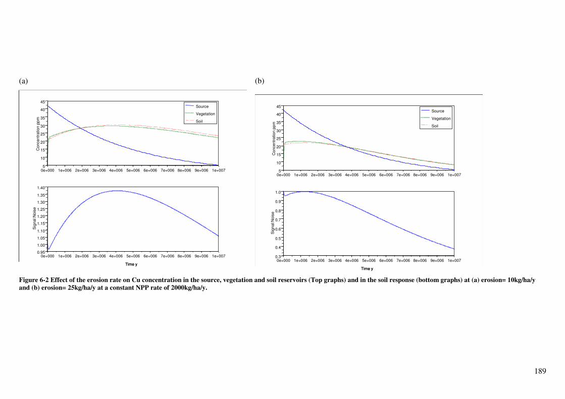
189

(a)

0e+000 1e+006 2e+006 3e+006 4e+006 5e+006 6e+006 7e+006 8e+006 9e+006 1e+0075

10

15

20

25

30

35

40

45

Co

nce

ntr

atio

n p

pm

Source

Vegetation

Soil

0e+000 1e+006 2e+006 3e+006 4e+006 5e+006 6e+006 7e+006 8e+006 9e+006 1e+0070.95

1.00

1.05

1.10

1.15

1.20

1.25

1.30

1.35

1.40

Time y

Sig

nal:N

ois

e

0e+000 1e+006 2e+006 3e+006 4e+006 5e+006 6e+006 7e+006 8e+006 9e+006 1e+0075

10

15

20

25

30

35

40

45

Co

nce

ntr

atio

n p

pm

Source

Vegetation

Soil

0e+000 1e+006 2e+006 3e+006 4e+006 5e+006 6e+006 7e+006 8e+006 9e+006 1e+0070.95

1.00

1.05

1.10

1.15

1.20

1.25

1.30

1.35

1.40

Time y

Sig

nal:N

ois

e

(b)

0e+000 1e+006 2e+006 3e+006 4e+006 5e+006 6e+006 7e+006 8e+006 9e+006 1e+0075

10

15

20

25

30

35

40

45

Co

nce

ntr

atio

n p

pm

Source

Vegetation

Soil

0e+000 1e+006 2e+006 3e+006 4e+006 5e+006 6e+006 7e+006 8e+006 9e+006 1e+0070.3

0.4

0.5

0.6

0.7

0.8

0.9

1.0

Time yS

ign

al:N

ois

e

0e+000 1e+006 2e+006 3e+006 4e+006 5e+006 6e+006 7e+006 8e+006 9e+006 1e+0075

10

15

20

25

30

35

40

45

Co

nce

ntr

atio

n p

pm

Source

Vegetation

Soil

0e+000 1e+006 2e+006 3e+006 4e+006 5e+006 6e+006 7e+006 8e+006 9e+006 1e+0070.3

0.4

0.5

0.6

0.7

0.8

0.9

1.0

Time yS

ign

al:N

ois

e

Figure 6-2 Effect of the erosion rate on Cu concentration in the source, vegetation and soil reservoirs (Top graphs) and in the soil response (bottom graphs) at (a) erosion= 10kg/ha/y

and (b) erosion= 25kg/ha/y at a constant NPP rate of 2000kg/ha/y.

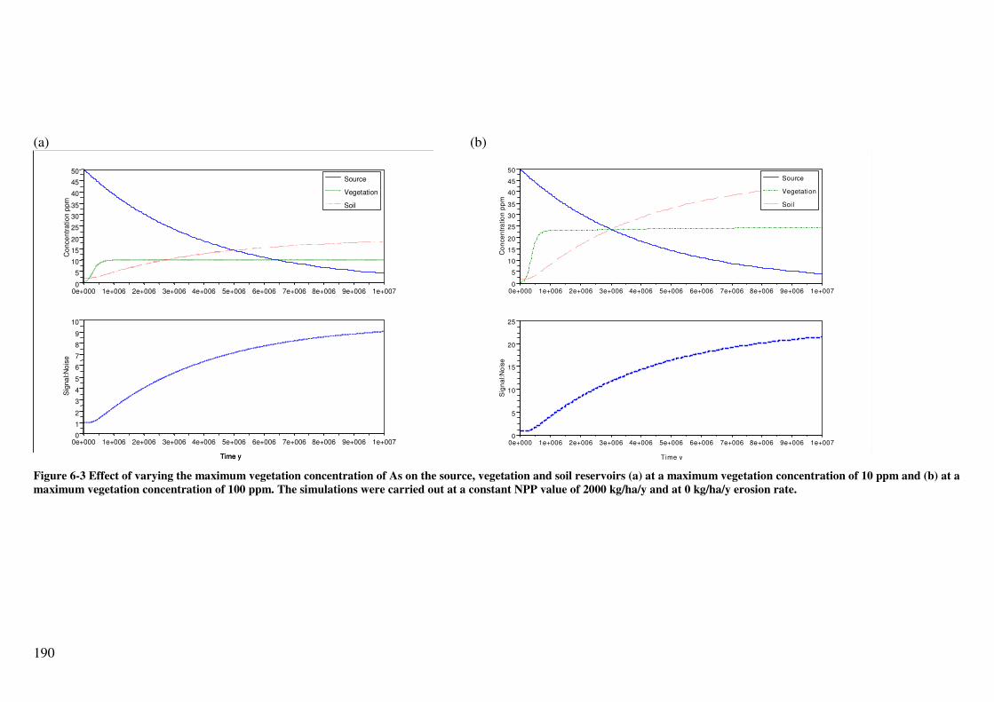
190

(a)

0e+000 1e+006 2e+006 3e+006 4e+006 5e+006 6e+006 7e+006 8e+006 9e+006 1e+0070

5

10

15

20

25

30

35

40

45

50

Co

nce

ntr

atio

n p

pm

Source

Vegetation

Soil

0e+000 1e+006 2e+006 3e+006 4e+006 5e+006 6e+006 7e+006 8e+006 9e+006 1e+0070

1

2

3

4

5

6

7

8

9

10

Time y

Sig

na

l:N

ois

e

0e+000 1e+006 2e+006 3e+006 4e+006 5e+006 6e+006 7e+006 8e+006 9e+006 1e+0070

5

10

15

20

25

30

35

40

45

50

Co

nce

ntr

atio

n p

pm

Source

Vegetation

Soil

0e+000 1e+006 2e+006 3e+006 4e+006 5e+006 6e+006 7e+006 8e+006 9e+006 1e+0070

1

2

3

4

5

6

7

8

9

10

Time y

Sig

na

l:N

ois

e

(b)

0e+000 1e+006 2e+006 3e+006 4e+006 5e+006 6e+006 7e+006 8e+006 9e+006 1e+0070

5

10

15

20

25

30

35

40

45

50

Co

nce

ntr

atio

n p

pm

Source

Vegetation

Soil

0e+000 1e+006 2e+006 3e+006 4e+006 5e+006 6e+006 7e+006 8e+006 9e+006 1e+0070

5

10

15

20

25

Time y

Sig

na

l:N

ois

e

Figure 6-3 Effect of varying the maximum vegetation concentration of As on the source, vegetation and soil reservoirs (a) at a maximum vegetation concentration of 10 ppm and (b) at a

maximum vegetation concentration of 100 ppm. The simulations were carried out at a constant NPP value of 2000 kg/ha/y and at 0 kg/ha/y erosion rate.

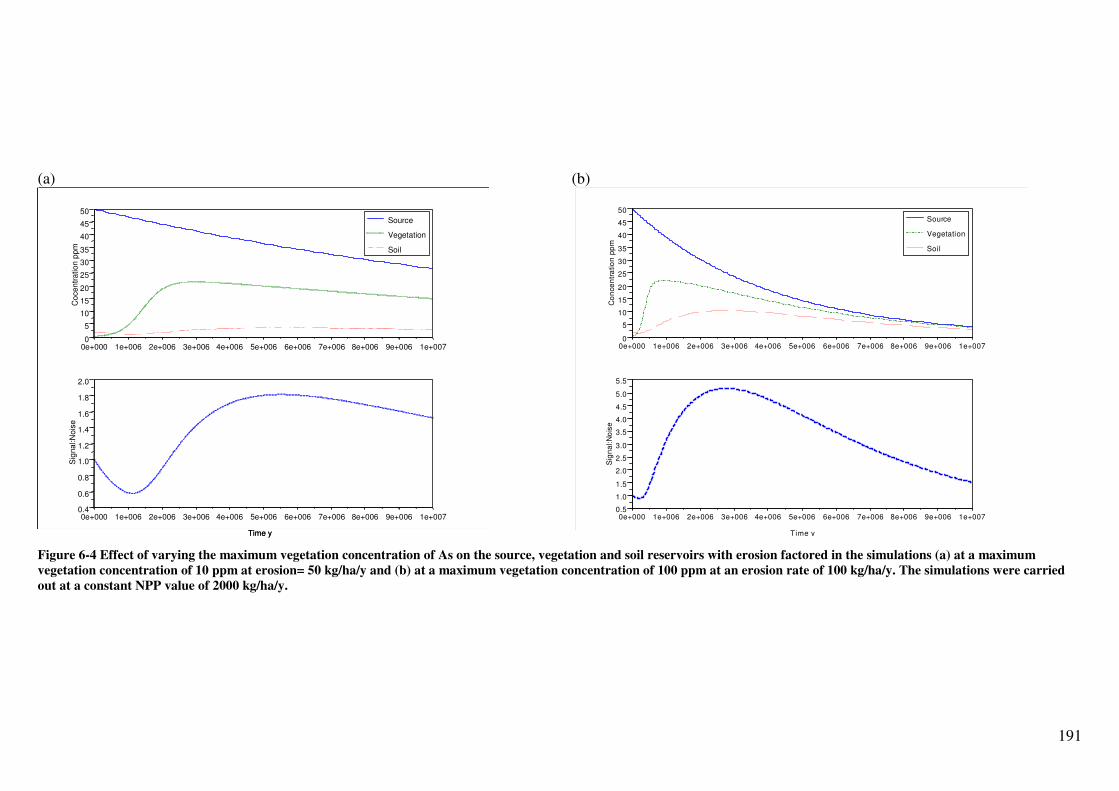
191

(a)

0e+000 1e+006 2e+006 3e+006 4e+006 5e+006 6e+006 7e+006 8e+006 9e+006 1e+0070

5

10

15

20

25

30

35

40

45

50

Co

cen

tra

tion

ppm

Source

Vegetation

Soil

0e+000 1e+006 2e+006 3e+006 4e+006 5e+006 6e+006 7e+006 8e+006 9e+006 1e+0070.4

0.6

0.8

1.0

1.2

1.4

1.6

1.8

2.0

Time y

Sig

na

l:N

ois

e

0e+000 1e+006 2e+006 3e+006 4e+006 5e+006 6e+006 7e+006 8e+006 9e+006 1e+0070

5

10

15

20

25

30

35

40

45

50

Co

cen

tra

tion

ppm

Source

Vegetation

Soil

0e+000 1e+006 2e+006 3e+006 4e+006 5e+006 6e+006 7e+006 8e+006 9e+006 1e+0070.4

0.6

0.8

1.0

1.2

1.4

1.6

1.8

2.0

Time y

Sig

na

l:N

ois

e

(b)

0e+000 1e+006 2e+006 3e+006 4e+006 5e+006 6e+006 7e+006 8e+006 9e+006 1e+0070

5

10

15

20

25

30

35

40

45

50

Co

nce

ntr

atio

n p

pm

Source

Vegetation

Soil

0e+000 1e+006 2e+006 3e+006 4e+006 5e+006 6e+006 7e+006 8e+006 9e+006 1e+0070.5

1.0

1.5

2.0

2.5

3.0

3.5

4.0

4.5

5.0

5.5

Time y

Sig

na

l:N

ois

e

Figure 6-4 Effect of varying the maximum vegetation concentration of As on the source, vegetation and soil reservoirs with erosion factored in the simulations (a) at a maximum

vegetation concentration of 10 ppm at erosion= 50 kg/ha/y and (b) at a maximum vegetation concentration of 100 ppm at an erosion rate of 100 kg/ha/y. The simulations were carried

out at a constant NPP value of 2000 kg/ha/y.

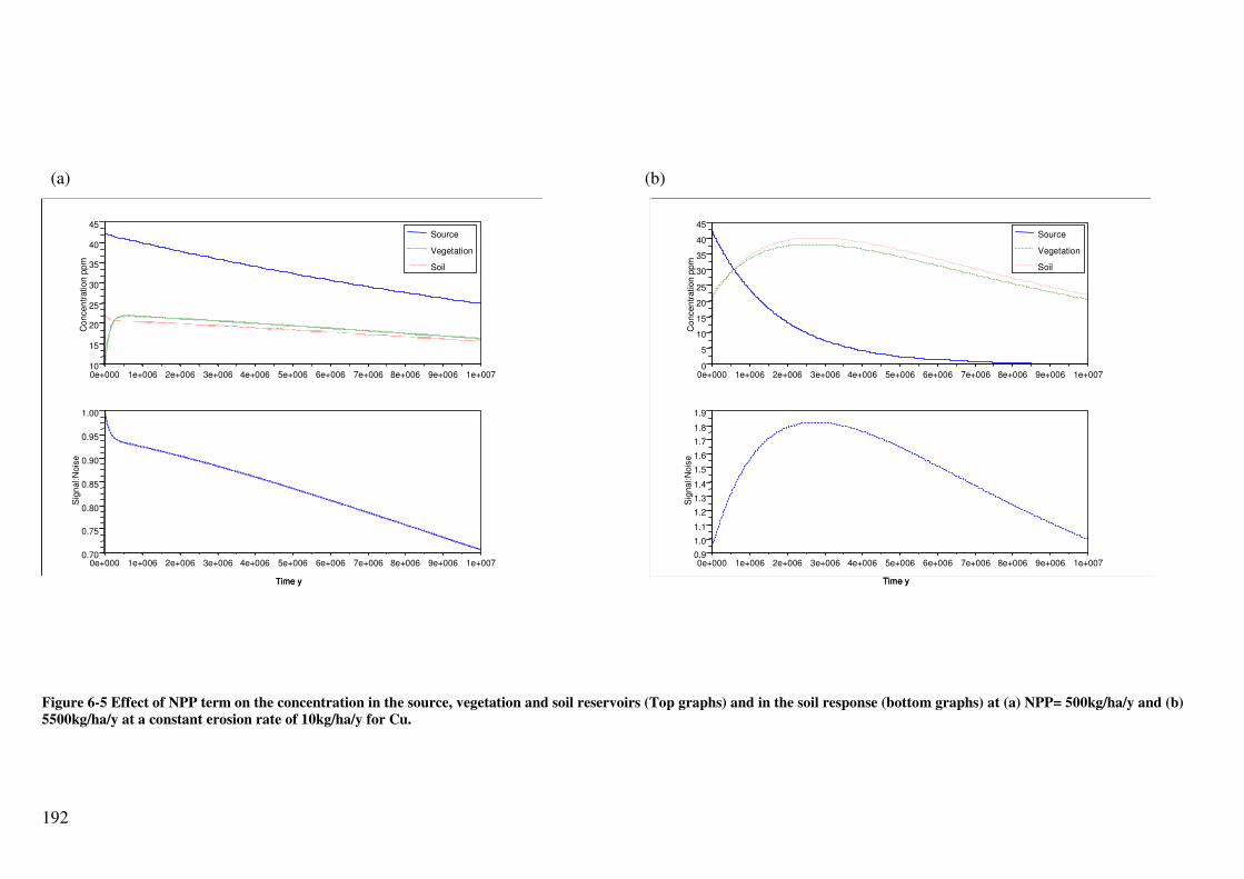
192

(a)

0e+000 1e+006 2e+006 3e+006 4e+006 5e+006 6e+006 7e+006 8e+006 9e+006 1e+00710

15

20

25

30

35

40

45

Co

ncen

tratio

n p

pm

Source

Vegetation

Soil

0e+000 1e+006 2e+006 3e+006 4e+006 5e+006 6e+006 7e+006 8e+006 9e+006 1e+0070.70

0.75

0.80

0.85

0.90

0.95

1.00

Time y

Sig

nal:N

ois

e

0e+000 1e+006 2e+006 3e+006 4e+006 5e+006 6e+006 7e+006 8e+006 9e+006 1e+00710

15

20

25

30

35

40

45

Co

ncen

tratio

n p

pm

Source

Vegetation

Soil

0e+000 1e+006 2e+006 3e+006 4e+006 5e+006 6e+006 7e+006 8e+006 9e+006 1e+0070.70

0.75

0.80

0.85

0.90

0.95

1.00

Time y

Sig

nal:N

ois

e

(b)

0e+000 1e+006 2e+006 3e+006 4e+006 5e+006 6e+006 7e+006 8e+006 9e+006 1e+0070

5

10

15

20

25

30

35

40

45

Co

ncen

tratio

n p

pm

Source

Vegetation

Soil

0e+000 1e+006 2e+006 3e+006 4e+006 5e+006 6e+006 7e+006 8e+006 9e+006 1e+0070.9

1.0

1.1

1.2

1.3

1.4

1.5

1.6

1.7

1.8

1.9

Time y

Sig

nal:N

ois

e

0e+000 1e+006 2e+006 3e+006 4e+006 5e+006 6e+006 7e+006 8e+006 9e+006 1e+0070

5

10

15

20

25

30

35

40

45

Co

ncen

tratio

n p

pm

Source

Vegetation

Soil

0e+000 1e+006 2e+006 3e+006 4e+006 5e+006 6e+006 7e+006 8e+006 9e+006 1e+0070.9

1.0

1.1

1.2

1.3

1.4

1.5

1.6

1.7

1.8

1.9

Time y

Sig

nal:N

ois

e

Figure 6-5 Effect of NPP term on the concentration in the source, vegetation and soil reservoirs (Top graphs) and in the soil response (bottom graphs) at (a) NPP= 500kg/ha/y and (b)

5500kg/ha/y at a constant erosion rate of 10kg/ha/y for Cu.

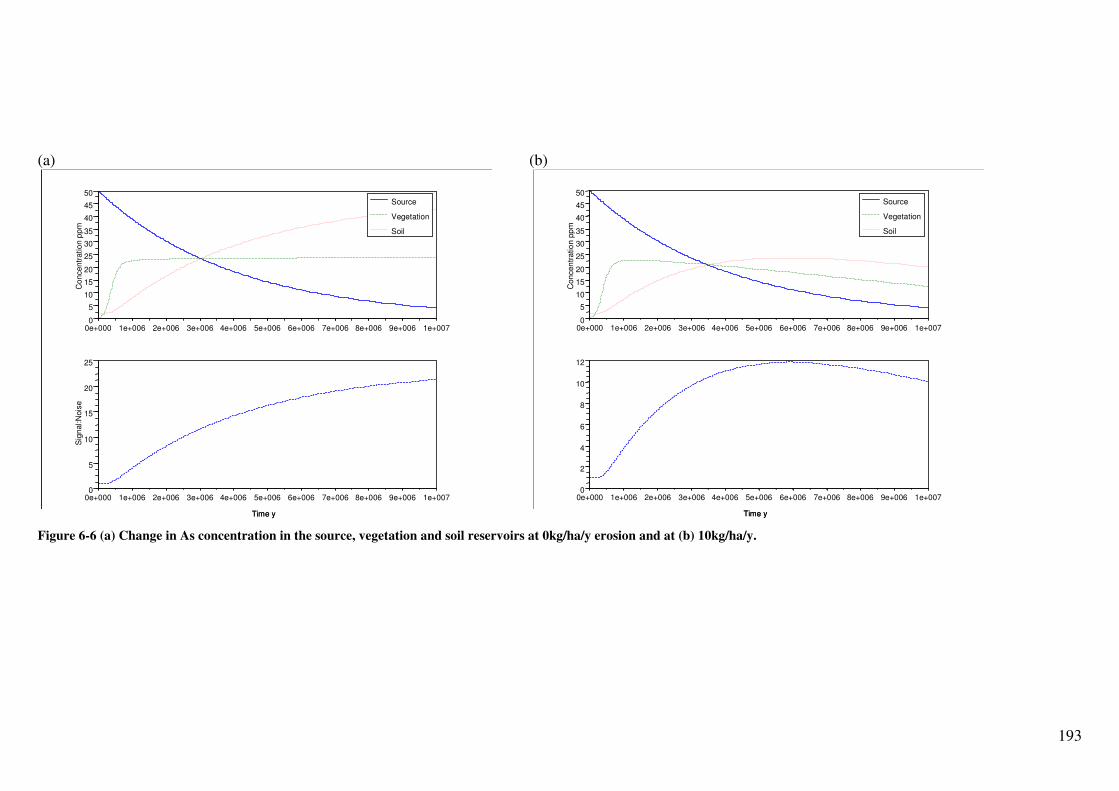
193

(a)

0e+000 1e+006 2e+006 3e+006 4e+006 5e+006 6e+006 7e+006 8e+006 9e+006 1e+0070

5

10

15

20

25

30

35

40

45

50

Co

ncen

tratio

n p

pm

Source

Vegetation

Soil

0e+000 1e+006 2e+006 3e+006 4e+006 5e+006 6e+006 7e+006 8e+006 9e+006 1e+0070

5

10

15

20

25

Time y

Sig

nal:N

ois

e

0e+000 1e+006 2e+006 3e+006 4e+006 5e+006 6e+006 7e+006 8e+006 9e+006 1e+0070

5

10

15

20

25

30

35

40

45

50

Co

ncen

tratio

n p

pm

Source

Vegetation

Soil

0e+000 1e+006 2e+006 3e+006 4e+006 5e+006 6e+006 7e+006 8e+006 9e+006 1e+0070

5

10

15

20

25

Time y

Sig

nal:N

ois

e

(b)

0e+000 1e+006 2e+006 3e+006 4e+006 5e+006 6e+006 7e+006 8e+006 9e+006 1e+0070

5

10

15

20

25

30

35

40

45

50

Con

cen

tratio

n p

pm

Source

Vegetation

Soil

0e+000 1e+006 2e+006 3e+006 4e+006 5e+006 6e+006 7e+006 8e+006 9e+006 1e+0070

2

4

6

8

10

12

Time y

0e+000 1e+006 2e+006 3e+006 4e+006 5e+006 6e+006 7e+006 8e+006 9e+006 1e+0070

5

10

15

20

25

30

35

40

45

50

Con

cen

tratio

n p

pm

Source

Vegetation

Soil

0e+000 1e+006 2e+006 3e+006 4e+006 5e+006 6e+006 7e+006 8e+006 9e+006 1e+0070

2

4

6

8

10

12

Time y

Figure 6-6 (a) Change in As concentration in the source, vegetation and soil reservoirs at 0kg/ha/y erosion and at (b) 10kg/ha/y.

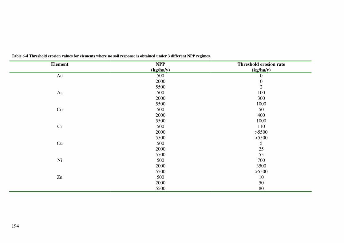
194

Table 6-4 Threshold erosion values for elements where no soil response is obtained under 3 different NPP regimes.

Element NPP

(kg/ha/y)

Threshold erosion rate

(kg/ha/y)

Au 500

2000

5500

0

0

2

As 500

2000

5500

100

300

1000

Co 500

2000

5500

50

400

1000

Cr 500

2000

5500

110

>5500

>5500

Cu 500

2000

5500

5

25

55

Ni 500

2000

5500

700

3500

>5500

Zn 500

2000

5500

10

50

80

195

6.3.2. Key variables influencing the development of biogeochemical signatures

From the differential equation modelling exercises, the development of biogeochemical

anomalies in the surface environment can be narrowed down to three key variables:

1. Deep uptake flux (bioavailability/ element abundance/ NPP)

2. Erosional flux

3. Maximum plant concentration

In terms of accumulative fluxes, the size of the deep uptake flux relative to the shallow

uptake flux is crucial. The differential equation model is particularly sensitive to the size

of the deep uptake flux, as seen by the large difference in modelling outputs between the

Au simulation (small deep uptake flux: k1 = 9 × 10-10

) and the Ni simulation (large deep

uptake flux, k1 = 4.7 × 10-7

). If the deep uptake flux is small, plant shallow uptake

initially depletes the soil reservoir (see the simulations for As above). Adding an

erosional flux enhances the depletion of the soil. Interestingly, although the deep biotic

uptake flux is dependent on the net primary productivity, the model is not as sensitive to

NPP as it is to the deep uptake or the erosional flux for elements at the two extremes

(Au, at the low end and Ni and Cr at the high end) of the deep uptake flux range. It can

also be concluded from the differential equation model that the bioavailability of

elements will affect the formation of soil anomalies, with the more abundant elements

such as Ni and Cr more rapidly forming a soil anomaly. However, the size of the soil

response (ie., signal : noise or response ratio) will also be off-set by the size of the

background concentration, hence for example in the Cu simulation, because of the

abundance of Cu in the surface soil, the corresponding soil response is low (refer to

Figure 5-11).

Soil erosion is the second process that is crucial to the development of biogeochemical

anomalies in the surficial environment. Pedogenetic modelling has also shown erosion

to be a significant factor controlling soil development (Brimhall et al. 1987; Minasny et

al. 1999; Minasny et al. 2001). Our model shows that if the deep uptake flux is small

relative to the erosional flux, as it is for the Au simulation, then any erosion in the

simulation will result in net loss from the soil, with no soil anomaly formed.

Furthermore, the Cu and As simulations show that erosion controls the development of

both soil and vegetation anomalies. Due to the feedback loop between the vegetation

196

and the soil in the shallow uptake flux, loss through soil erosion will eventually lead to

the decay of the vegetation anomaly as well. As erosion depletes the soil reservoir, the

deep uptake of elements into the vegetation reservoir subsequently becomes insufficient

to balance the loss flux through erosion, as the source gets depleted simultaneously.

The rapid cycling between the plant and surface soil implies that the maximum

allowable plant concentration is the third variable that exerts significant control over

biogeochemical anomalies. As our simulations show, at low maximum plant

concentrations, accumulation in the soil is significantly reduced, particularly if erosion

is present. Subsequently, the soil anomaly forms at a slower rate. Conversely, if the

maximum plant concentration was raised, the rate of accumulation in the soil

subsequently becomes greater.

Finally, the rate constants used in our simulations were derived using approximations of

variables obtained in the literature. For example, the proportion of root biomass found

as deep roots was used as a proxy for the partitioning co-efficient between deep and

shallow uptake. As a result, the rate expressions are approximations only. Further

improvements for these rate constants should be sought, either through experimentation

or field studies, particularly with regard to the deep uptake flux and the erosional flux.

6.3.3. Application to mineral exploration

The outcomes of our modelling work, specifically, the derivation of the three main

variables controlling the development of biogeochemical anomalies, has several

ramifications for mineral exploration. Most significantly, first order differential

modelling confirmed that biogeochemical anomalies have a limited life-span, after the

deposition of the transported overburden. Hence, if an exploration survey was carried

out either at the formative stage or at the decay stage of the soil anomaly, the soil

response may be less obvious. The biogeochemical cycling of elements may also

explain the lack of a soil anomaly observed in other biogeochemical studies (Cohen et

al. 1999; Butt et al. 2003) and in our own field sites in Berkley and Torquata in Western

Australia. The simulations also indicated that soil anomalies may not always form by

biotic uplift, and are dependent on the deep uptake flux and ultimately, the size of the

source reservoir. Hence for elements with a small source reservoir (e.g. As) the

formation of a soil anomaly through biotic uplift is less likely, especially under active

erosion. However, a small vegetation anomaly may be present, which may make

197

interpretation of soil and vegetation sampling results difficult. Accordingly, because of

different erosional regimes operating at different points in the landscape,

biogeochemical anomalies may not be as pronounced where erosion is dominant (e.g.

on hillslopes cf. flat, stable parts of the landscape). This is likely to have an impact on

the process of choosing a suitable exploration strategy for a particular environment.

Finally, the simulations show that the mineralisation reservoir eventually decays and

thus also has a limited life-span, the length of which depends on the size of the relative

loss fluxes. The surface geochemical signature could sometimes “outlive” the

mineralisation, particularly if the source is low grade mineralisation. This could lead to

the detection of false anomalies, where little or no mineralisation is present underneath

the geochemical halo. The Au bound in the near surface calcrete at Torquata could, for

example, be the surface expression of a long decayed mineralisation at depth.

6.4. Further work

Future directions can be taken to further develop the differential equation model. For

example, depth of the transported overburden could be included as a variable. However,

there is as yet no explicit relationship that has been defined between depth of

overburden and the development of geochemical signatures in its surface (see Chapter 3

and 4) (also see Lintern (2001)). The differential equation model could also be

expanded into a 2-dimensional model by inclusion of a lateral plant cycling flux,

whereas currently, the spatial dimensions of the model are implicit and constrained by

the input parameters (e.g. volume of regolith, volume of soil anomaly). As plants take

up nutrients, lateral transport of elements in the soil occurs through redistribution by the

surficial cycling flux (Rose et al. 1979; Buxbaum et al. 2001). Lateral redistribution of

elements as a biogenic phenomenon is recognised in the exploration literature and is

discussed in more detail in Chapter 2 (Rose et al. 1979) Inclusion of a lateral transport

flux would therefore enable the development of a more realistic first order differential

equation model. Using variable NPP and erosion rates based upon palaeoclimatic data

may enable more accurate modelling of soil anomaly formation than using present day

values. Validation of the model is still needed and measurements of some of the fluxes

estimated from literature values are still required. For example, the loss fluxes of

erosion and leaching could be quantified if suitable methodology is applied (e.g.

Matschonat et al. 1997; Tipping et al. 2003; Cammeraat 2004; Chirino et al. 2006). The

need to quantify the maximum allowable plant concentration in the plant reservoir also

198

opens up future research pathways into determining toxicity levels in plants of some of

the non-biologically essential elements but which may be important ore-related

elements like Au.

6.5. Conclusions

The differential equation model suggested that soil anomalies are indeed transient

geochemical features at the Earth’s surface, as discussed earlier in our rudimentary mass

balance (Chapter 2). Simulations showed no Au anomalism developed in the soil by

biotic uplift. The outcome for the differential equation model for Au also contradicts

field observations. This led us to conclude that there must be an underlying variable that

was not accounted for in the differential equation model. From the simulations, three

key variables that affect the development of biogeochemical anomalies were narrowed

down: Deep plant uptake flux, maximum plant concentration and erosion. The outcomes

of the modelling exercises thus point to an optimal time in which to sample soil and

vegetation media when the response relative to background concentration is high.

Alternatively, our models indicate that the optimal conditions under which a

biogeochemical anomaly may be produced in semi-arid environments that are i) metal-

rich source, ii) high concentrations of metal(s) in plant tissue, iii) high net primary

productivity and iv) low erosion rates.

199

CHAPTER SEVEN

CONCLUSIONS

7. Summary and General Conclusions

It is remarkable how intricately linked the biosphere is with the physical environment.

Evidence from a vast body of literature shows that plants are effective agents in

redistributing trace elements found in the regolith directly into the surface soils. Plants

can also accumulate high concentrations of non-essential trace elements in their tissues.

Their ability to sample large volumes of regolith and accumulate large concentrations of

trace elements makes them powerful tools for mineral exploration surveys, particularly

in areas of transported cover. Based on this information, we examined the hypothesis

that plants act as conduits between a buried ore deposit and the surface soil by

transporting elements from depth into the soil through plant return. Within a sufficient

time-frame (ca. 106

y) and under suitable conditions, this mechanism suggests that

plants could deposit higher concentrations of ore-related elements relative to

background from depth into the soil. Biotic uplift of ore related elements from depth

could explain why soils developed on barren, exogenic overburden sometimes show a

geochemical signature apparently derived from an underlying ore deposit.

It is considered that the research objectives set out in Chapter 1 were satisfactorily met

in this work. The charcoal experiment showed that natural charcoal can absorb large

concentrations of metals but the fractionation of these metals could not be identified by

a sequential extraction scheme. This shows that sequential extraction data cannot

currently be used as evidence for or against the biogeochemical hypothesis for soil

anomaly formation. However, this does not preclude that a carefully designed sequential

extraction study, focusing on specific metals that are bound to organic matter and key

plant species that specifically uptake these metals may help further unravel the link

between vegetation and soil anomalies. The success of these types of studies would

hinge on identifying key plant species that accumulate specific metals. The results of the

charcoal experiment reinforce the importance of understanding trace element sinks with

a biological origin.

In Chapter 2, a basic model of trace element cycling was developed as the starting

ground to conceptualise the main fluxes and reservoirs that are central to the formation

200

of soil anomalies through biotic uplift. Through a scoping study of the literature on

vegetation and vegetation community characteristics, and biogeochemical exploration

case studies, there is sufficient evidence to give cause to our central hypothesis that

plants transport and deposit high concentrations of elements in the surface soil from

depth. Based on approximate mass-balance calculations, we came up with specific

hypotheses regarding the formation of soil geochemical anomalies by biotic means,

namely:

1) The existence of soil anomalies depends on the balance between ecosystem net

primary productivity and trace element losses through soil erosion and leaching.

2) Accumulation in soils will be favoured for more bioavailable elements.

3) Soil anomalies may only be transient geological features, depending on the

relative rates of trace element accumulation in, and loss from, surface soils.

Analyses of soil and vegetation samples for Au and a suite of other trace elements at

two Au prospects in Western Australia were carried out to complement the initial

theoretical groundwork. An analytical method for analysis of Au in vegetation samples

by ashing and aqua regia dissolution followed by graphite furnace- atomic absorption

spectrophotometry (GF-AAS) was also successfully developed and was integral to the

field component of this study. Generally, the soils and eucalypt trees growing over both

sites showed high responses to the buried mineralisation at Berkley and Au associated

with calcrete at Torquata. Sampling at Torquata showed a general correlation between

the occurrence of Au accumulation in the vegetation and the regolith/calcrete Au. The

co-occurrence of high Au concentrations in surface soils in certain parts of the

landscape at the contrasting Berkley and Torquata prospects, however, makes the issue

of whether the vegetation was acquiring Au from depth inconclusive. The vegetation at

both sites may well be recycling the Au only from a pre-existing soil anomaly already at

the surface developed by prior, unknown processes. At the Berkley field site, the soils

are enriched in Au and various other trace elements only in the top few metres; between

this enriched zone and the regolith anomaly lies tens of metres thick of barren

transported material and the buried, in situ material. This paradox coupled with the fact

that the vegetation reflected the geochemical characteristics of the buried lithology may

represent indirect evidence of plant transport for Au from depth into the surface. In

addition, distinct anomalies of elements such as Cr, Ni and As were detected in the

vegetation samples over certain lithological contacts, which suggests greater mobility of

elements in solution along these contacts. To our knowledge, the correlation of trace

201

element signature in vegetation with lithology and over different lithological contacts

has not previously been reported in the literature.

The prospect at Torquata, in contrast, is unusual in that almost all the anomalous Au is

present in near-surface calcrete, which has formed within the transported overburden.

Initial drilling at the site had detected no Au in the bedrock. There were thus two main

unknowns with the Torquata site: the origins of the Au in near-surface calcrete, and; the

mechanism for Au association with the calcrete. Plant uplift was proposed as a central,

unifying mechanism of Au transport into the surface environment: both in extracting Au

from an unknown source mineralisation and in the subsequent association of the Au

with the calcrete. Secondarily, a biogeochemical survey of the site could help locate the

source of Au in the calcrete, which might have been beyond the extent of the drill lines.

The current biogeochemical study could not, however, trace the source of the Au in the

calcrete. The Au could not have originated from the in situ material because there is no

evidence of bedrock mineralisation. Torquata sits within the Eucla Basin, a Cainozoic

drainage basin known for its placer Au and heavy mineral sands deposits. It is possible

that the source of the calcrete Au may itself be the remnant hydromorphic dispersion

trail and/or detrital Au transported from another unknown, inland source of Au

(possibly from the Yilgarn Craton). The large rare earth anomalies found in the

Torquata soils seem to corroborate this story. The strong correlations between Ca and

Au in the leaf and litter samples do, however, suggest that the vegetation may have had

a role in the transport of Au in the regolith and association of the Au in the calcrete. The

strong correlation between Li and Au in the surface soils also suggests the highly

mobile nature of Au in the surface soils (Note: no relationship between Li and Au was

found at Berkley).

The potential for biotic uplift of trace elements from depth was assessed using a simple

but mechanistic numerical model, based on coupled differential equations which

described trace element fluxes. Biotic uplift of several ore elements at depth and their

eventual deposition into surface soils was successfully simulated using first order

differential equation modelling. The key fluxes leading to the development of soil

anomalies as identified from the initial theoretical model in Chapter 2 were quantified.

The outcome from rate expressions developed from the calculated fluxes enabled us to

narrow down three key variables that control the formation of soil anomalies in semi-

arid environments: 1) the size of the deep uptake flux, 2) the maximum concentration in

202

the plant reservoir and 3) the erosional regime. More importantly, as we proposed

earlier in Chapter 2, the differential equation model showed that soil anomalies are

likely to have a limited “life-span” as a result of the changes in the relative sizes of the

net accumulative and loss fluxes in the system. Thus, the soil never attains equilibrium

over the time of the peak anomalism, in the model because elements are continually

added from the source and lost from the system through erosion and leaching. Unless

there is no erosion, the concept that a soil anomaly has a limited life-span has direct

implications to the usefulness of soils as sampling media for exploration surveys in

covered terrane.

An interesting outcome of the modelling was the possibility that soil anomalies for Au

were unlikely to form in soils by biotic uplift at Berkley; the calculated contribution

from the biotic uplift flux for Au is simply too small, even with minimal loss from the

soil through erosion and leaching. This contradicts the high Au concentrations measured

in some of the surface soil samples at the Berkley site, as well as the mass balance in

Chapter 2. The disparity between field observation and the simulations may indicate

that either an unknown variable is missing from the numerical model or that biotic

uplift, acting in tandem with other mechanisms of transport, covered briefly in Chapter

2, may be responsible for the high concentrations of Au in the soils at Berkley. An

alternative interpretation of the modelling would mean that it would take an inordinately

long time for Au (>100 My; much longer than the overburden itself has been in place),

or any other elements found in low concentrations at the source, to accumulate in soils

solely through biotic uplift. Without an age estimate of the transported overburden, it is

difficult to determine the time taken for accumulation in the soil. Only further

development and validation of the numerical model, with refinement in the values used

for the fluxes, as well as an age estimate for the transported overburden, may help

resolve this problem (see next section). The sensitivity of the model to the three key

factors above also implies that the likelihood of anomaly formation will increase with

the bioavailability of an element, which agrees with the hypothesis generated from the

initial mass balance work in Chapter 2. In an environment like Torquata, where the Au

may be locked up in the calcrete for part of the time, the rate of accumulation of Au by

biotic uplift may be different in the surface soils. Calcrete in this case acts as an

additional reservoir for Au. Additional research problems are also raised; for example,

the bioavailability of Au bound to calcrete is not currently known. Conceivably, if the

203

calcrete bound Au were less bioavailable than in free solution, this feeds back into the

vegetation reservoir where less Au would be recycled at the surface.

The modelling indicated further that over time, the source or mineralisation eventually

decays. This implies that the mineralisation source also has a limited life-span, as biotic

uplift in combination with other loss fluxes such as deep drainage and diffusion,

eventually depletes the source, or at least its bioaccessible component. The depletion of

the source may explain the lack of a spatially continuous Au anomaly at depth at

Torquata. If only a small concentration of hydrologically transported Au was

accumulated in the present day in situ materials, prior to the deposition of the

overburden, depletion of this source could readily occur, especially if groundwater flow

is actively dispersing the Au.

Currently in Australia, we are just beginning to compile a dataset for biogeochemical

exploration through the pioneering work of Butt, Lintern, Cohen and Anand and others

(e.g. Hill and Hulme). Although biogeochemical exploration is well established in the

northern hemisphere, there is no equivalent depth of understanding for application of

the technique to Australian ecosystems. Data from this study contributes to the current,

limited database of biogeochemical exploration studies in depositional areas of

Australia. In addition, the first, mechanistic biogeochemical model for the formation of

soil anomalies in transported overburden through biogenic means has been developed in

this thesis.

On a final note, future research into the role of biota in shaping the physical and

chemical attributes of the surface soil environment (and as we have shown in this work,

to some extent, the deeper regolith) will undoubtedly hinge on finding evidence for the

operation of the deep biotic uplift flux. In an exploration context, future research into

the area may not be as rewarding given the numerous difficulties in finding evidence for

this flux. Finding evidence for the deep biotic uplift flux requires specific environmental

conditions in which it is assumed to dominate over other vertical transport mechanisms

and the presence of a barren overburden. Without the use of innovative and technically

advanced methods (such as isotopic analyses; see below), it is insufficient to merely

infer the operation of the biotic uplift flux from indirect, empirical evidence. Probably

the most problematic issue with indirect evidence is that once ore elements have

accumulated in the surface soils, it is difficult to tell if the associated high response in

204

the vegetation is a result of the vegetation having acquired the elements from depth in

the regolith or from the soil. This is not to say however, that future research in the deep

biotic uplift by vegetation is not worthwhile in other contexts. The idea that the

vegetation had as much a hand in determining the characteristics of soils as the soil had

in determining the vegetation type growing on it has far reaching research implications

in the fields of ecology and pedogenesis (see Taylor et al. 1991; Ollier 2001; Pate et al.

2001; Verboom et al. 2006).

7.1. Implications for Future Research

7.1.1. Development of soil geochemical anomalies in transported

overburden

There was no conclusive proof in our field study at Berkley (or at Torquata) that plants

were taking up Au from depth in the buried regolith. We could not rule out

unequivocally that the plants were merely recycling the Au in the surface. Based on our

model of soil anomaly formation, once a mature soil anomaly develops, it is difficult to

distinguish biotic uplift as a causative mechanism. Isotopic analyses of plant tissues

may help inform the issue, for example with the use of oxygen or strontium isotopes.

Under certain circumstances, analysis of Sr-isotope ratios within plant tissues can be

used (Capo et al. 1998; Poszwa et al. 2002). The basis for use of Sr as an ecosystem

tracer is that the isotope ratios can be used to distinguish between an atmospherically

derived source and that of a lithologically derived source. Since Sr isotopic ratios do not

change in plants, the plant retains the distinct isotopic signature of the Sr-source.

Therefore, an indication of where the plant derives its ultimate source of Sr can be

obtained and hence be used as a proxy to similar elements such as Ca (Stewart et al.

1998). Isotopic analyses will also inform the modelling work in determining the

partitioning of the net plant uptake flux between that from the surficial soil horizons and

the deep regolith.

Studying the effect of overburden depth and time since deposition of the overburden

would also greatly aid our current knowledge of the way soil anomalies form in

transported overburden. Conceivably, biogenic transport of elements into the surface

soils will be limited by the depth of the overburden. There is however, no evidence yet

in the literature (see Chapter 2) or from our own field work to suggest that there is a

205

systematic relationship between overburden depth and the development of soil and

vegetation anomalies. Hence, for future studies, a detailed soil pit study with larger

depths may be required to study the effect of depth on the trace element distribution in

the profile. Following the mass balance in Lintern (2007), dating of the overburden

material may also assist our modelling efforts to get an idea of the time constraints

within which soil anomalies may have formed. This will then enable us to define an

upper limit of time within which biotic uplift of elements can occur, thereby giving us

an actual field-measured value to compare out model outputs to.

In addition, validation of the model requires rigorous testing in the field. Multi-element

measurements carried out on the soil solution (both within the rhizosphere and in the

lower parts of the soil-profile) would give a better indication of the leaching losses to

groundwater and also to the lateral spread of elements from the mineralised region.

Once the elements reach the surface soil, they will be redistributed laterally by surface

recycling by plants, which can be experimentally determined (Buxbaum et al. 2001).

7.1.2. Biogeochemical modelling

Modelling is an essential tool to help bridge the nexus between the generation of results

from field-based work and the application of these results universally (Schlesinger

1991). Models can aid in the generation of fresh field hypotheses (Phillips 2007) to test

the biogeochemical method on the ground, with the ultimate goal of developing

exploration strategies for similar environments based on a biogeochemical mechanism

for soil anomaly formation. Future directions can still be taken with our differential

modelling work. For example, depth of the transported overburden could be included as

a variable. Studies have shown the importance of transported overburden depth on the

abiotic development of geochemical anomalies in the surficial environment (Hamilton

1998; Cameron et al. 2004). However, there is as yet no explicit relationship that has

been defined between depth of overburden and the development of geochemical

signatures in its surface (see Chapter 3 and 4) (also see Lintern (2001)). Further, the

differential model could also be developed into a 2- or 3-dimensional model by

inclusion of a lateral plant cycling flux. As plants take up nutrients and other elements,

lateral transport of elements in the soil occurs through redistribution by surficial cycling

fluxes and hydrological flows (Rose et al. 1979; Buxbaum et al. 2001). Lateral

redistribution of elements as a biogenic phenomenon is recognised in the exploration

literature (Rose et al. 1979). Inclusion of a lateral transport flux would therefore enable

206

the development of a more realistic differential equation model which simulates

formation and decay of soil anomalies in two dimensions (concentration and horizontal

distance, as opposed to the single concentration dimension in this work). Improvements

in the input values for the maximum concentration in the plant reservoir could still be

made (Dasgupta-Schubert et al. 2007). For example, toxic concentrations could be

determined experimentally in plants for some of the non-biologically essential elements,

but which may be important ore-related elements, such as Au. Net primary productivity

and erosion parameters adjusted to the palaeoclimatic history of the study site may

enable more realistic simulations of soil anomaly development.

207

REFERENCES

ABENSPERG-TRAUN, M. (1992). "Biomass of surface-foraging ants (Formicidae) in

four bushland habitats in the wheatbelt of Western Australia." Journal of the

Royal Society of Western Australia, 75: 25-32.

ACKAY, M., LERMI, A. and VAN, A. (1998). "Biogeochemical exploration for

massive sulphide deposits in areas of dense vegetation: an orientation survey

around the Kankoy Deposit (Trabzon, NE Turkey)." Journal of Geochemical

Exploration, 63: 173-187.

AHMED, A. K., JOHNSON, K. A., SONNEVELD, C. and BERHOYEN, M. N. J.

(2000). "Growing Australian native edible plants using hydroponic techniques."

Acta Horticulturae, 511: 225-231.

ALLISON, G. B. and HUGHES, M. W. (1972). "Comparison of recharge to

groundwater under pasture and forest using environmental tritium." Journal of

Hydrology, 17: 81-95.

ALLOWAY, B. J. (1995). 3. The origins of heavy metals in soils. In. B. J. Alloway,

(ed.) 3. Heavy Metals in Soil. London, Blackie Academic and Professional.

ANAND, R. R. (2001). "Evolution, classification and use of ferruginous materials in

gold exploration, Yilgarn Craton, Western Australia." Geochemistry:

Exploration, Environment, Analysis, 1: 221-236.

ANAND, R. R. and CORNELIUS, M. (2004). Vegetation and soil expression of the

Jaguar base metal deposit, Yilgarn Craton.In: Regolith 2004, Adelaide, CRC

Leme, 7-8.

ANAND, R. R. and PAINE, M. (2002). "Regolith geology of the Yilgarn Craton,

Western Australia: implications for exploration." Australian Journal of Earth

Sciences, 49: 3-162.



Western Australia: a contribution towards understanding metal transportation


ANAND, R. R., PHANG, C., WILDMAN, J. E. and LINTERN, M. J. (1997). "Genesis

of some calcretes in the southern Yilgarn Craton, Western Australia." Australian

Journal of Earth Sciences, 44: 87-103.

ANAND, R. R., WILDMAN, J. E., VARGA, Z. S. and PHANG, C. (2001). "Regolith

evolution and geochemical dispersion in transported and residual regolith-

Bronzewing gold deposit." Geochemistry: Exploration, Environment, Analysis,

1: 265-276.

ANDRADE, W. O., MACHESKY, M. L. and ROSE, A. W. (1991). "Gold distribution

and mobility in the surficial environment, Carajas region, Brazil." Journal of

Geochemical Exploration, 40: 95-114.

ARNE, D. C., STOTT, J. E. and WALDRON, H. M. (1999). "Biogeochemistry of the

Ballarat East goldfield, Victoria, Australia." Journal of Geochemical


ATTIWILL, P. M. and LEEPER, G. W. (1987). Forest Soils and Nutrient Cycles.

Melbourne University Press.

AZIMI, S., CAMBIER, P., LECUYER, I. and THEVENOT, D. (2004). "Heavy metal

determination in atmospheric deposition and other fluxes in Northern France

agrosystems." Water, Air and Soil Pollution, 157: 295-313.

BARBIERO, L., PARATE, H.R., DESCLOITRES, M., BOST, B., FURIAN, S.,

MOHAN KUMAR, M.S., KUMAR, C., BRUAN, J-J. (2007). "Using a

208

structural approach to identify relationships between soil and erosion in a semi-

humid forested area, South India." Catena, 70: 313-329.

BATISTA, M. J., ABREU, M. M. and SERRANO PINTO, M. (2007).

"Biogeochemistry in Neves Corvo mining region, Iberian Pyrite Belt, Portugal."


BIERMAN, P. R., REUTER, J. M., PAVICH, M., GELLIS, A. C., CAFFEE, M. W.

and LARSEN, J. (2005). "Using cosmogenic nuclides to contrast rates of erosion

and sediment yield in a semi-arid, arroyo-dominated landscape, Rio Puerco

Basin, New Mexico." Earth Surface Processes and Landforms, 30: 935-953.

BRIMHALL, G. H. and DIETRICH, W. E. (1987). "Constitutive mass balance between

chemical composition, volume, density, porosity, and strain in metasomatic

hydrochemical systems: results on weathering and pedogenesis." Geochemica et

Cosmochimica Acta, 51: 567-587.

BRITT, A. F., SMITH, R. E. and GRAY, D. J. (2001). "Element mobilities and the

Australian regolith- a mineral exploration perspective." Marine Freshwater

Research, 52: 25-39.




235.

BUREAU OF METEOROLOGY AUSTRALIA (2007). “Climate of Kalgoorlie-

Boulder”.

Available from: <http://www.bom.gov.au/weather/wa/kalgoorlie/climate.shtml>

[16/9/2007].



158-165.

BUSS, H. L., BRUNS, M. A., SCHULTZ, M. J., MOORE, J., MATHUR, C. F. and

BRANTLEY, S. L. (2005). "The coupling of biological iron cycling and mineral

weathering during saprolite formation, Luquillo Mountains, Puerto Rico."

Geobiology, 3: 247-260.

BUTT, C. M. R. and ZEEGERS, H., (eds) (1992). Regolith Exploration Geochemistry

in Tropical and Subtropical Terrains, Vol.4. Handbook of Exploration

Geochemistry. Amsterdam, Elsevier.

BUTT, C. M. R., LINTERN, M. J. and ANAND, R. R. (2000). "Evolution of regoliths

and landscapes in deeply weathered terrain- implications for geochemical

exploration." Ore Geology Reviews, 16: 167-183.

BUTT, C. R. M. (1992a). Chapter I.1: Climate, geomorphological environment and

geochemical dispersion models. In. C. R. M. Butt and H. Zeegers, (eds) Chapter

I.1: Climate, geomorphological environment and geochemical dispersion

models. Amsterdam, Elsevier. 4: 3-24.

BUTT, C. R. M. (1992b). Chapter I.6: Physical Weathering and Dispersion. In. C. R. M.

Butt and H. Zeegers, (eds) Chapter I.6: Physical Weathering and Dispersion.

Amsterdam, Elsevier. 4: 96-113.

BUTT, C. R. M. (1992c). Chapter III.3: Semiarid and arid terrains. In. C. R. M. Butt

and H. Zeegers, (eds) Chapter III.3. Semiarid and arid terrains. Amsterdam,

Elsevier. 4: 365-367.

BUTT, C. R. M. and DRIES, S. (2003). Fender Gold Deposit, Cue, Western Australia,

CRC LEME.

BUTT, C. R. M. and GOLE (1985). "Helium in soil and overburden gas as an

exploration pathfinder-an assessment." Journal of Geochemical Exploration, 24:

141-173.

209

BUTT, C. R. M. and SMITH, R. E. (1980). "Conceptual models in exploration

geochemistry, Australia." Journal of Geochemical Exploration, 12: 89-365.

BUXBAUM, C. A. Z., NOWAK, C. A. and WHITE, E. H. (2001). "Long-term soil

nutrient dynamics and lateral nutrient movement in fertilized and unfertilized red

pine plantations." Biogeochemistry, 55: 269-292.




135-145.




CAMMERAAT, E. L. H. (2004). "Scale dependent thresholds in hydrological and

erosion response of a semi-arid catchment in southeast Spain." Agriculture

ecosystems and environment, 104: 317-332.

CANADELL, J., JACKSON, R. B., ERLERINGER, J. R., MOONEY, H. A., SALA, O.

E. and SCHULZE, E. D. (1996). "Maximum rooting depth of vegetation types at

the global scale." Oecologia, 108: 583-595.

CAPO, R. C., STEWART, B. W. and CHADWICK, O. A. (1998). "Strontium isotopes

as tracers of ecosystem processes: theory and methods." Geoderma, 82: 197-225.

CENTRE FOR EXPLORATION TARGETTING (2007). Greenfields exploration.

Perth, Western Australia, UWA. 2007.

CHAO, T. T. and ZHOU, L. (1983). "Extraction techniques for selective dissolution of

amorphous iron oxides from soils and sediments." Soil Science Society of

America Proceedings, 47: 225-232.

CHIMNER, R. A. and COOPER, D. J. (2004). "Using stable oxygen isotopes to

quantify the water source used for transpiration by native shrubs in the San Luis

Valley, Colorado, U.S.A." Plant and Soil, 260: 225-236.

CHIRINO, E., BONET, A., BELLOT, J. and SANCHEZ, J. R. (2006). "Effects of 30-

year-old Aleppo pine plantations on runoff, soil erosion, and plant diversity in a

semi-arid landscape in south eastern Spain." Catena, 65: 19-29.

CHUNG, E. H., LEE, J. S., CHON, H. T. and SAGER, M. (2005). "Environmental

contamination and bioaccessibility of arsenic and metals around the Dongjeong

Au-Ag-Cu mine, Korea." Geochemistry: Exploration, Environment, Analysis, 5:

69-74.

COHEN, D. R., SHEN, X. C., DUNLOP, A. C. and RUTHERFORD, N. F. (1998). "A

comparison of selective extraction soil geochemistry and biogeochemistry in the

Cobar area, New South Wales." Journal of Geochemical Exploration, 61: 173-

189.

COHEN, D. R., SILVA-SANTISTEBAN, C. M., RUTHERFORD, N. F., GARNETT,

D. L. and WALDRON, H. M. (1999). "Comparison of vegetation and stream

sediment geochemical patterns in northeastern New South Wales." Journal of


CONN, E. E., MASLIN, B. R., CURRY, S. and CONN, M. E. (1985). "Cyanogenesis in

Australian species of Acacia. Survey of herbarium specimens and living plants."

Western Australian Herbarium Research Notes, 10: 1-60.

COVENTRY, R. J., HOLT, J. A. and SINCLAIR, D. F. (1988). "Nutrient cycling by

mound-building termites in low-fertility soils of semi-arid tropical Australia."

Australian Journal of Soil Research, 26: 375-390.

CRAW, D., YOUNGSON, J. H. and LECKIE, D. A. (2006). "Transport and

concentration of detrital gold in foreland basins." Ore Geology Reviews, 28:

417-430.

210

DAKORA, F. D. and PHILLIPS, D. A. (2002). "Root exudates as mediators of mineral

acquisition in low-nutrient environments." Plant and Soil, 245: 35-47.

DALRYMPLE, J. J., COHEN, D. R. and GATEHOUSE, S. G. (2005). "Optimisation of

partial extraction chemistry for buffered acetate and hydroxylamine buffers."

Geochemistry: Exploration, environment, analysis, 5: 279-285.

DASGUPTA-SCHUBERT, N., WHELAN, T., REYES, M. A. and LLOREN, C.

(2007). "Light quanta modulated characteristics of Ni uptake by Brassica juncea

seedlings: the interdependence of plant metal concentration and biomass."

International Journal of Phytoremediation, 9: 207-225.

DAWES, W. R., GILFEDDER, M., STAUFFACHER, M., et al. (2002). "Assessing the

variability of recharge reduction of dryland salinity control: Wanilla, Eyre

Peninsula." Australian Journal of Soil Research, 40: 1407-1424.

DORR, H. (1995). "Application of 210Pb in soils." Journal of Paleolimnology, 13: 157-

168.



15: 437-452.

DUNN, C. E. (1986). Application of biogeochemical methods to mineral exploration in

the boreal forests of central Canada. In. D. Carlisle, W. L. Berry, I. R. Caplan

and J. R. Watterson, (eds) Application of biogeochemical methods to mineral

exploration in the boreal forests of central Canada. Englewood Cliffs, NJ,

Prentice-Hall: 133-149.

DUNN, C. E. and HOFFMAN, E. (1986). "Multi-element study of vegetation from a

zone of rare-earth rich allanite and apatite in northern Saskatchewan, Canada."

Applied Geochemistry, 1: 375-381.

DUNN, C. E. and RAY, G. E. (1995). "A comparison of lithogeochemical and

biogeochemical patterns associated with gold mineralization in mountainous

terrain of southern British Columbia." Economic Geology, 90: 2232-2243.

DYCK, W. and MEILLEUR, G.A. (1972). "Soil gas sampler for difficult overburden."


EASTHAM, J., GREGORY, P. J. and WILLIAMSON, D. R. (2000). "A spatial analysis

of lateral and vertical fluxes of water associated with a perched watertable in a

duplex soil." Australian Journal of Soil Research, 38: 879-890.

EILERS, V. H. M., CARTER, R. C. and RUSHTON, K. R. (2007). "A single layer soil

water balance model for estimating deep drainage (potential recharge): An

application to cropped land in semi-arid North-east Nigeria." Geoderma, 140:

119-131.

ELDRIDGE, D. J. and MYERS, C. A. (1998). "Enhancement of soil nutrients around

nest entrances of the funnel ant Aphaenogaster barbigula (Myrmicinae) in semi-

arid eastern Australia." Australian Journal of Soil Research, 36: 1009-1017.

FLYNN, T. M. and SOUTHWELL, I. A. (1987). "Cyanogenesis in the genus Zieria."

Phytochemistry, 26: 1669-1672.

FORTESCUE, J. A. C. (1975). "The use of landscape geochemistry to process

exploration geochemical data." Journal of Geochemical Exploration, 4: 3-13.

FOULDS, W. and CARTWRIGHT, Z. (1985). "Polymorphisms for cyanogenesis in

Lotus australis Andr. from coastal dunes at Kalbarri, Western Australia." Lotus

Newsletter, 16: 17-26.

FREYSSINET, P. and FARAH, A. S. (2000). "Geochemical mass balance and

weathering rates of ultramafic schists in Amazonia." Chemical Geology, 170:

133-151.

FREYSSINET, P. and ITARD, Y. (1997). Geochemical mass balance of gold under

various tropical weathering conditions: Application to exploration. In:

211

Proceedings of Exploration 97: Fourth Decennial Conference on Mineral

Exploration.

FROUZ, M., HOULEC, M. and KALCIK, J. (2003). "The effect of Lasius niger

(Hymenopter, Formicidae) ant nest on selected soil chemical properties."

Pedobiologia, 47: 205-212.

GELINAS, Y. and SCHMIT, J.-P. (1998). "Estimation of bulk atmospheric deposition

of major and trace elements to a rural watershed." Atmospheric Environment,

72: 1473-1483.

GLASER, B., BALASHOV, E., HAUMAIER, L., GUGGENBERGER, G. and ZECH,

W. (2002). "Black carbon in density fractions of anthropogenic soils of the

Brazillian Amazon region." Organic Geochemistry, 31: 668-679.

GOVERNMENT OF SOUTH AUSTRALIA (2007). Primary Industries and Resources

SA: Mineral Sands: Eucla Basin.

GOVETT, G. J. S. (1976). "Detection of deeply buried and blind sulphide deposits by

measurement of H+ and conductivity of closely spaced surface soil samples."


GOVETT, G. J. S. and ATHERDEN, P. R. (1987). "Electrogeochemical patterns in

surface soils - Detection of blind mineralization beneath exotic cover, Thalanga,

Queensland, Australia." Journal of Geochemical Exploration, 28: 201-218.

GRAY, D. J. (2001). "Hydrogeochemistry of the Yilgarn Craton." Geochemistry:


GRAY, D. J., BUTT, C. R. M. and LAWRENCE, L. M. (1992). Chapter V.3: The

geochemistry of gold in lateritic terrains. In. C. R. M. Butt and H. Zeegers, (eds)

Chapter V.3: The geochemistry of gold in lateritic terrains. Amsterdam,

Elsevier. 4: 461-498.

GRIERSON, P. F. and ADAMS, M. A. (1999). "Nutrient cycling and growth in forest

ecosystems of south western Australia: Relevance to agricultural landscapes."

Agroforestry Systems, 45: 215-244.

GRIMES, D. J., FICKLIN, W. H., MEIER, A. L. and MCHUGH, J. B. (1995).

"Anomalous gold, antimony, arsenic, and tungsten in ground water and alluvium

around disseminated gold deposits along the Getchell Trend, Humboldt County,

Nevada." Journal of Geochemical Exploration, 52: 351-371.

GUSTAFSSON, J. P., PECHOVA, P. and BERGGREN, D. (2003). "Modeling metal

binding to soils: the role of natural organic matter." Environmental Science and

Technology, 37: 2467-2774.

HALL, G. E. M. and PELCHAT, P. (2005). "The design and application of sequential

extractions for mercury, Part 2. Readsorption of mercury onto the sample during

leaching." Geochemistry: Exploration, environment, analysis, 5: 115-121(7).

HALL, G. E. M., VAIVE, J. E., BEER, R. and HOASHI, M. (1996). "Selective leaches

revisited, with emphasis on the amorphous Fe oxyhydroxide phase extraction."


HALSTEAD, M. J. R., CUNNINGHAME, R. G. and HUNTER, K. A. (2000). "Wet

deposition of trace metals to a remote site in Fiordland, New Zealand."

Atmospheric Environment, 34: 665-676.

HAMILTON, S. M. (1998). "Electrochemical mass-transport in overburden: a new

model to account for the formation of selective leach geochemical anomalies in

glacial terrain." Journal of Geochemical Exploration, 63: 155-172.

HARPER, R. J. and GILKES, R. J. (1994). "Evaluation of the 137Cs technique for

estimating wind erosion losses for some sandy Western Australian soils."


HART, D. M. (1995). "Litterfall and decomposition in the Pillaga State Forests, New

South Wales, Australia." Australian Journal of Ecology, 20: 266-272.

212

HEIMSATH, A. M., DIETRICH, W. E., NISHIIZUMI, K. and FINKEL, R. C. (1997).

"The soil production function and landscape equilibrium." Nature, 388: 358-388.

HERAIL, G., LAGOS, J. and VIVALLO, W. (1999). "Gold dispersion in Andean desert

environments (Atacama, Chile)." Journal of Geochemical Exploration, 66: 427-

439.

HILL, S and HULME, K ()

HILLER, D. A. and BRUMMER, G. W. (1996). "Electron microprobe studies on soil

samples with varying heavy metal contamination. 2. Contents of heavy metals in

aggregations of humic substances, litter residues and charcoal particles."

Zeitschrift fur Pflanzenernahrung und Bodenkunde, 160: 47-55.

HOU, B. and WARLAND, I. (2005). "Heavy mineral sands potential of the Eucla Basin

in South Australia." MESA Journal, 37: 4-12.

ISIK ECE, O., SCHROEDER, P.A. (2007). "Clay mineralogy and chemistry of

halloysite and alunite in the Turplu area, Balikesir, Turkey." Clay and Clay

Minerals, 55: 18-35.

JACOB, R. H. and PEET, R. L. (1989). "Acute oxalate toxicity of sheep associated with

slender iceplant (Mesembryanthemum nodiflorum)." Australian Veterinary

Journal, 66: 91-92.

JAKOB, M., MCKENDRY, I. and LEE, R. (2003). "Long-term changes in rainfall

intensities in Vancouver, British Columbia." Canadian Water Resources

Journal, 28: 587-604.

JAYKO, A. S. (2005). "Late Quaternary denudation, Death and Panamint Valleys,

eastern California." Earth Science Reviews, 73: 271-289.

JIA, Y. F., STEELE, C. J., HAYWARD, I. P. and THOMAS, K. M. (1998).

"Mechanisms of adsorption of gold and silver species on activated carbons."

Carbon, 36: 1299-1308.



JOHNSON, D. W. and VAN HOOK, R. I. (1989). Analysis of Biogeochemical Cycling

Processes in Walker Branch Watershed. Springer-Verlag, New York.

JORDAN, C. F. (1983). Productivity of tropical rain forest ecosystems and the

implications for their use as future wood and energy sources. In. F. B. Golley,

(ed.)Tropical Rainforest Ecosystems. Structure and Function. Amsterdam,

Netherlands, Elsevier Science Publishers. 14A of 'Ecosystems of the World':

117-136.

JULL, A. J. T., DONAHUE, D. J., BROSHI, M. and TOV, E. (1995). "Radiocarbon

dating of scrolls and linen fragments from the Judedan Desert." Radiocarbon,

37: 11-19.

KABATA-PENDIAS, A. and PENDIAS, H. (1991). CRC Press: Trace elements in soils

and plants, 2nd Edition. CRC Press, Baco Raton.

KARAJAS, J. (1999). Detecting base-metal mineralisation through glacial till cover:

MMI case histories from Northern Sweden. AIG Bulletin. 30: 69-80.

KASTE, J. M., HEIMSATH, A. M. and BOSTICK, B. C. (2007). "Short-term soil

mixing quantified with fallout radionuclides." Geology, 35: 243-246.

KEELING, J. (2004). Metal ion dispersion through transported cover at Moonta, South

Australia. In. I. C. Roach, (ed.) Regolith 2004. CRC LEME. 2004: 161-165.

KELEPERTSIS, A., ALEXAKIS, D. and KITA, I. (2001). "Environmental

geochemistry of soils and waters of Susaki area, Korinthos, Greece."

Environmental Geochemistry and Health, 23: 117-135.

KELLEY, D. L. and KELLEY, K. D. (2006). "Beyond the obvious limits of ore

deposits: The use of mineralogical, geochemical and biological features for the

remote detection of mineralisation." Economic Geology, 101: 729-752.

213

KERSTEN, M. and FORSTNER, U. (1989). Speciation of trace elements in sediments.

In. G. E. Batley, (ed.) Speciation of trace elements in sediments. CRC Press:

245-317.

KIZITO, F., SENE, M., DRAGILA, M. I., et al. (2007). "Soil water balance of annual

crop–native shrub systems in Senegal's Peanut Basin: The missing link."

Agricultural Water Management, 90: 137-148.

KOBER, F., IVY-OCHSC, S., SCHLUNEGGERE, F., BAUR, H., KUBIK, P. W. and

WIELER, R. (2007). "Denudation rates and a topography-driven rainfall

threshold in northern Chile: Multiple cosmogenic nuclide data and sediment

yield budgets." Geomorphology, 83: 97-120.

KRACHLER, M., MOHL, C., EMONS, H. and SHOTYK, W. (2003). "Atmospheric

Deposition of V, Cr, and Ni since the Late Glacial: effects of climatic cycles,

human impacts, and comparison with crustal abundances." Environmental

Science and Technology, 37: 2658-2667.

KUMA, J. S. (2007). "Hydrogeological study of the Tarkwa mining district, Ghana."

Bull Eng Geol Env, 66: 89-99.

LEE, K. E. (1983). Soil animals and pedological processes. In: Soils: An Australian

Viewpoint. Melbourne/London, CSIRO/Academic Press: 629-644.

LEE, K. E. and WOOD, T. G. (1971). Termites and soils. In: Termites and soils.

London, Academic Press.

LEYBOURNE, M. I. and CAMERON, E. M. (2007). Source, transport, and fate of

rhenium, selenium, molybdenum, arsenic, and copper in groundwater associated

with porphyry-Cu deposits, Atacam Desert, Chile. Chemical Geology. 2007.

LI, J. (2002). Silver Adsorption/Desorption on Soil Constituents and Fractionation of

Silver and other Trace Elements in Soils. Soil Science and Plant Nutrition. Perth,

University of Western Australia.

LI, J., RATE, A. W. and GILKES, R. B. (2003). "Fractionation of trace elements in

non-agricultural Australian soils." Australian Journal of Soil Research, 41: 1389-

1402.

LI, J., RATE, A. W. and GILKES, R. B. (2004). "Silver ion desorption kinetics from

iron oxides and soil organic matter: effect of adsorption period." Australian

Journal of Soil Research, 42: 59-67.

LIETH, H. (1975). Primary production of the major vegetation units of the world. In. H.

Lieth and R. H. Whittaker, (eds) Primary Productivity of the Biosphere. New

York, Springer-Verlag: 203-215.

LINDBERG, S. E., HARISS, R. C., HOFFMAN JR., W. A., LOVETT, G. M. and

TURNER, R. R. (1989). Chapter 4: Atmospheric chemistry, deposition, and

canopy interactions. In. D. W. Johnson and R. I. Van Hook, (eds) Analysis of

Biogeochemical Cycling Processes in Walker Branch Watershed. New York,

Springer-Verlag: 96-163.

LINTERN, M. J. (1999). Study of the distribution of gold in soils at Mt Hope, Western

Australia. Wembley, Western Australia, Cooperative Research Centre for

Landscape Evolution and Mineral Exploration.

LINTERN, M. J. (2001). "Exploration for gold using calcrete- lessons from the Yilgarn

Craton, Western Australia." Geochemistry: Exploration, Environment, Analysis,

1: 237-252.




LINTERN, M. J. and BUTT, C. R. M. (1998). The distribution of gold and other

elements in soils at the Granny Smith gold deposit, Western Australia.

214

Wembley, Western Australia, Cooperative Research Centre for Landscape

Evolution and Mineral Exploration: 73.

LINTERN, M. J., BUTT, C. R. M. and SCOTT, K. M. (1997). "Gold in vegetation and

soil- three case studies from the goldfields of southern Western Australia."


LINTERN, M. J., SHEARD, M. J. and CHIVAS, A. R. (2006). "The source of the

pedogenic carbonate associated with gold-calcrete anomalies in the western

Gawler Craton, South Australia." Chemical Geology, 235: 299-394.

LOBRY DE BRUYN, L. A. and CONACHER, A. J. (1990). "The role of termites and

ants in soil modification: a review." Australian Journal of Soil Research, 28: 55-

93.

LOBRY DE BRUYN, L. A. and CONACHER, A. J. (1994a). "The bioturbation activity

of ants in agricultural and naturally vegetated habitats in semi-arid

environments." Australian Journal of Soil Research, 32: 555-570.

LOBRY DE BRUYN, L. A. and CONACHER, A. J. (1994b). "The effect of ant

biopores on water infiltration in soils in undisturbed bushland and in farmland in

a semi-arid environment." Pedobiologia, 38: 193-207.

LOBRY DE BRUYN, L. A. and CONACHER, A. J. (1995a). "Soil modification by

termites in the central wheatbelt of Western Australia." Australian Journal of

Soil Research, 33: 179-193.

LOPEZ-BERMUDEZ, R., ROMERO-DIAZ, A., MARTINEZ-FERNANDEZ, J. and

MARTINEZ-FERNANDEZ, J. (1998). "Vegetation and soil erosion under a

semi-arid Meditarranean climate: a case study from Murcia (Spain)."

Geomorphology, 24: 51-58.

LOW, V. H. K. and THOMSON, J. A. (1990). "Cyanogenesis in Australian bracken

(Pteridium esculentum): distribution of cyanogenic phenotypes and factors

influencing activity of the cyanogenic glucosidase." Aias Occasional

Publications, 40: 105-111.

MALAJCZUK, N. and CROMACK, K., JR. (1982). "Accumulation of calcium oxalate

in the mantle of ectomycorrhizal roots of Pinus radiata and Eucalyptus

marginata." New Phytologist, 92: 527-531.

MALYUGA, D. P. (1964). Biogeochemical Methods of Prospecting, Authorised

translation from the Russian. Consultants Bureau, New York.

MANN, A. W., BIRRELL, R. D., FEDIKOW, M. A. F. and DE SOUZA, H. A. F.

(2005). "Vertical ionic migration: mechanisms, soil anomalies and sampling

depth for mineral exploration." Geochemistry: Exploration, Environment,

Analysis, 5: 201-214.

MARSCHNER, H. (1995). Chapter 16: Adaptation of Plants to Adverse Chemical Soil

Conditions. In: Mineral Nutrition of Higher Plants. London, Academic Press:

596-680.

MASLIN, B. R., DUNN, J. E. and CONN, E. E. (1988). "Cyanogenesis in Australian

species of Acacia." Phytochemistry, 27: 421-428.

MATSCHONAT, G. and VOGT, R. (1997). "Assessment of a laboratory method to

obtain the equilibrium solution composition of forest soils." European Journal of

Soil Science, 48: 545-552.

MCCLELLAN, Y., AUGUST, R., GOSZ, J., et al. (2003). "Uptake rates of Thorium

progeny in a semiarid environment." Journal of Environmental Quality, 32:

1759-1763.




215




MCKEAGUE, J. A. (1967). "An evaluation of 0.1M pyrophosphate and pyrophosphate-

dithionite in comparison with oxalate as extractants of the accumulation

products in podzols and some other soils." Canadian Journal of Soil Science, 47:

95-99.

MCKENZIE, N., JACQUIER, D., ISBELL, R. and BROWN, K. (2004). Chapter 2: The

evolution of the Australian landscape. In: Australian Soils and Landscapes.

Collingwood, Australia, CSIRO Publishing: 33.

MILLIGAN, D. A. and MUHTADI, O. A. (1988). Chemical solution control. In. D. J.

A. van Zyl, I. P. G. Hutchison and J. E. Kiel, (eds) Introduction to Evaluation,

Design and Operation of Precious Metal Heap Leaching Projects. Littleton,

Colorado, Society of Mining Engineers: 275-292.

MINASNY, B. and MCBRATNEY, A. B. (1999). "A rudimentary mechanistic model

for soil production and landscape development." Geoderma, 90: 3-21.


for soil formation and landscape development II. A two-dimensional model

incorporating chemical weathering." Geoderma, 103: 161-179.

MUMM, A. S. and REITH, F. (2007). "Biomediation of calcrete at the gold anomaly of

the Barns prospect, Gawler Graton, South Australia." Journal of Geochemical


NIEROP, K. G. J. V. and VERSTRATEN, J. M. (2004). "Rapid molecular assessment

of the bioturbation extent in sandy soil horizons under pine using ester-bound

lipids by on-line thermally assisted hydrolysis and methylation-gas

chromatography/mass spectrometry." Rapid Commun. Mass Spectrom., 18:

1081-1088.

NISKAVAARA, H., KONTAS, E. and REIMANN, C. (2004). "Regional distribution

and sources of Au, Pd and Pt in moss and O-, B- and C-horizon podzol samples

in the European Arctic." Geochemistry: Exploration, Environment, Analysis, 4:

143-159.

NOLLER, B. N., WATTERS, R. A. and WOODS, P. H. (1997). "The role of

biogeochemical processes in minimising uranium dispersion from a mine site."


O'CONNELL, A. M., MALAJCZUK, N. and GAILITIS, V. (1983). "Occurrence of

calcium oxalate in karri (Eucalyptus diversicolor F. Muell.) forest ecosystems of

south western Australia." Oecologia, 56: 239-244.

PAIS, I. and JONES, J. B. (1997). The Handbook of Trace Elements. St. Lucie Press,

Boca Raton, FL, USA.

PARTON, W. J., STEWART, J. W. B. and COLE., C. V. (1988). "Dynamics of C, N, P

and S in grassland soils: a model." Biogeochemistry, 5: 109-131.

PASTOR-VILLEGAS, J., DURAN-VALLE, C. J., VALENZUELA-CALAHORRO, C.

and GOMEZ-SERRANO, V. (1998). "Organic chemical structure and shrinkage

of chars prepared from rockrose." Carbon, 36: 1251-1256.

PATE, J. S., JESCHKE, W. D., DAWSON, T. E., RAPHAEL, C., HARTUNG, W. and

BOWEN, B. J. (1998). "Growth and seasonal utilisation of water and nutrients

by Banksia prionotes." Australian Journal of Botany, 46: 511-532.

PATE, J. S., VERBOOM, W. H. and GALLOWAY, P. D. (2001). "Turner Review No.

4: Co-occurrence of Proteaceae, laterite and related oligotrophic soils:

coincidental associations or causative inter-relationships?" Australian Journal of

Botany, 49: 529-560.

216

PAUWELS, H., BAUBRON, J. C., FREYSSINET, P. and CHESNEAU, M. (1999).

"Sorption of metallic compounds on activated carbon: application to exploration

for concealed deposits in southern Spain." Journal of Geochemical Exploration,

66: 115-133.

PHILLIPS, J. D. (2007). Soil system modelling and generation of field hypotheses.

Geoderma, doi:10.106/j.geoderma.2007.07.01.

PILLANS, B. (1997). "Soil Development at Snail's Pace: Evidence from a 6 Ma Soil

Chronosequence on Basalt in North Queensland, Australia." Geoderma, 80: 117-

218.

PILLANS, B. (2007). "Pre-Quaternary landscape inheritance in Australia." Journal of

Quaternary Science, 22: 439-447.

POSZWA, A., DAMBRINE, E., FERRY, B., POLLIER, B. and LOUBET, M. (2002).

"Do tree roots provide nutrients to the tropical rainforest?" Biogeochemistry, 60:

97-118.

QUEREJETA, J. I., ESTRADA-MEDINA, H., ALLEN, M. F. and JIMINEZ-

OSORNIO, J. J. (2007). "Water source partitioning among trees growing on

shallow karst soils in a seasonally dry tropical climate." Oecologia, 152: 26-36.

RADFORD, N. W. and BURTON, P. E. (1999). "The geochemistry of transported

overburden: the time factor. An example from the Fender deposit, Big Bell,

Western Australia." Journal of Geochemical Exploration, 66: 71-83.

RAI, S. N. and PROCTOR, J. (1986). "Ecological studies on four rainforests in

Karnataka, India. I. Environment, structure, floristics and biomass. II. Litterfall."

Journal of Ecology, 74: 439-463.

RAICH, J. W. (1998). "Above ground productivity and soil respiration in three

Hawaiian rain forests." Forest Ecology and Management, 107: 309-318.

RAUPACH, M. (1962). "Solubility of simple aluminium compounds expected in soils I.

Hydroxides and oxyhydroxides." Australian Journals of Soil Research, 1: 28-35.

REA, A. W., LINDBERG, S. E. and KEELER, G. J. (2001). "Dry deposition and foliar

leaching of mercury and selected trace elements in deciduous forest throughfall."


READING, K. A. L., BROOKS, R. R. and NAIDU, S. D. (1987). "Biogeochemical

prospecting for gold in the Canadian Artic." Journal of Geochemical


REUTER, D. J. and ROBINSON, J. B., (eds) (1997). Plant Analysis: An Interpretation

Manual. Collingwood, Australia, CSIRO Publishing.

ROERING, J. J., ALMOND, P., TONKIN, P. J. and MCKEAN, J. (2002). "Soil

transport driven by biological processes over millenial timescales." Geology, 30:

1115-1118.

ROGERS, P. J. and DUNN, C. E. (1993). "Trace element chemistry of vegetation

applied to mineral exploration in eastern Nova Scotia, Canada." Journal of


RÖMHELD, V. (1991). "The role of phytosiderophores in acquisition of iron and other

micronutrients in graminacious species: an ecological approach." Plant and Soil,

130: 127-134.

ROSE, A. W., HAWKES, H. E. and WEBB, J. S. (1979). Geochemistry in Mineral

Exploration. Academic Press, London.

SAHOO, N. R. and PANDALAI, H. S. (2000). "Secondary geochemical dispersion in

the Precambrian auriferous Hutti-Maski schist belt, Raichur district, Karnataka,

India. Part I: anomalies of As, Sb, Hg and Bi in soil and groundwater." Journal

of Geochemical Exploration, 71: 269–289.

SAILEROVA, E. and FEDIKOW, M. A. F. (2004). "The effects of seasonal changes,

sample site drainage and tree morphology on trace element contents of black

217

spruce (Picea mariana (Mill.) BSP) crown twigs and outer bark." Geochemistry:


SALA, O. E., PARTON, W. J., JOYCE, L. A. and LAUENROTH, W. K. (1988).

"Primary production of the central grassland region of the United States."

Ecology, 60: 40-45.

SANDER, M. and PIGNATELLO, J. J. (2005). "Characterisation of charcoal adsorption

sites for aromatic compounds: insights drawn from single-solute and bi-solute

competitive experiments." Environmental Science and Technology, 39: 1606-

1615.

SANDVIG, R. M. and PHILLIPS, F. M. (2006). "Ecohydrological controls on soil

moisture fluxes in arid to semiarid vadose zones." Water Resources Research,

42: 8422-8422.

SAS INSTITUTE INC. (2006). SAS Enterprise Guide 4.1. Cary, NC, USA.

SCANLON, B. R., KEESE, K. E., FLINT, A. L., et al. (2006). "Global synthesis of

groundwater recharge in semiarid and arid regions." Hydrological Processes, 20:

3335-3370.

SCHENK, H. J. and JACKSON, R. B. (2002). "The global biogeography of roots."

Ecological Monographs, 72: 311-328.

SCHENK, H. J. and JACKSON, R. B. (2005). "Mapping the global distribution of deep

roots in relation to climate and soil characteristics." Geoderma, 126: 129-140.

SCHLESINGER, W. H. (1991). Biogeochemistry: An analysis of global change. San

Diego, California, Academic Press.




SERGEEV, N. B. and GRAY, D. J. (2001). "Gold mass balance in the regolith, Mystery

Zone, Mt Percy, Kalgoorlie, Western Australia." Geochemistry: Exploration,

Environment, Analysis, 1: 307-312.

SEYFRIED, M. S., SCHWINNING, S., WALVOORD, M. A., et al. (2005).

"Ecohydrological control of deep drainage in arid and semiarid regions."

Ecology, 86: 277-287.

SILCOCK, R. G. and SMITH, F. T. (1983). "Soluble oxalates in summer pastures on a

mulga soil." Tropical Grasslands, 17: 179-181.

SINGH, B. P., LEE, Y. I., PAWAR, J. S. and CHARAK, R. S. (2007). "Biogenic

features in calcretes developed on mudstone: Examples from Palaeogene

sequences of the Himalaya, India." Sedimentary Geology, 20: 149-156.

SKJEMSTAD, J. O., JANIK, L. J. and TAYLOR, J. A. (1998). "Non-living soil organic

matter: what do we know about it?" Australian Journal of Experimental

Agriculture, 38: 667-680.

SKJEMSTAD, J. O., REICOSKY, D. C., WILTS, A. R. and MCGOWAN, J. A. (2002).

"Charcoal carbon in U.S. agricultural soils." Soil Science Society of America

Journal, 66: 1249-1255.

STARR, M., LINDROOS, A., UKONMAANAHO, L., TARVAINEN, T. and

TANSKANEN, H. (2003). "Weathering release of heavy metals from soil in

comparison to deposition, litterfall and leaching fluxes in a remote boreal

coniferous forest." Applied Geochemistry, 18: 607-613.

STEDNICK, J. D. and RIESE, W. C. (1987). "Temporal variation of metal

concentrations in biogeochemical samples over the Royal Tiger Mine, Colorado,

Part II. Between-year variation." Journal of Geochemical Exploration, 27: 53-62.

STEWART, B. W., CAPO, R. C. and CHADWICK, O. A. (1998). "Quantitative

strontium isotope models for weathering, pedogenesis and biogeochemical

cycling." Geoderma, 82: 173-195.

218

STRETCH, R. C. and VILES, H. A. (2002). "The nature and rate of weathering by

lichens on lava flows on Lanzarote." Geomorphology, 47: 87-94.



STUMM, W. (1992). Chemistry of the Solid-water interface. John Wiley and Sons.

SYNMAN, H. A. (2005). "Rangeland degradation in a semi-arid South Africa—I:

influence on seasonal root distribution, root/shoot ratios and water-use

efficiency." Journal of Arid Environments, 60: 457-481.

TAYLOR, A. B. and VELBEL, M. A. (1991). "Geochemical mass balances and

weathering rates in forested watersheds of the southern Blue Ridge II. Effects of

botanical uptake terms." Geoderma, 51: 29-50.

THORNBER, M. R. (1992). Chapter I.5: The Chemical Mobility and Transport of

Elements in the Weathering Environment. In. C. R. M. a. Z. Butt, H., (ed.)

Regolith Exploration Geochemistry in Tropical and Subtropical Terrains.


TIPPING, E., RIEUWERTS, J., PAN, G., et al. (2003). "The solid-solution partitioning

of heavy metals (Cu, Zn, Cd, Pb) in upland soils of England and Wales."

Environmental Pollution, 125: 213-225.

VALENTE, I., MINSKI, M. J. and PETERSON, P. J. (1986). "Biogeochemical

exploration for gold at a site in the Cordillera Cantabrica, Spain." Journal of


VANDERMEER, J. (1981). Elementary mathematical ecology. John Wiley and Sons,

New York.

VELBEL, M. A. (1986). The mathematical basis for determining rates of geochemical

and geomorphic processes in small forested watersheds by mass balance:

examples and implications. In. S. M. Colman and D. P. Dethier, (eds) Rates of

Chemical Weathering in Rocks and Minerals. Orlando, Academic Press.

VELBEL, M. A. and PRICE, J. R. (2007). "Solute geochemical mass-balances and

mineral weathering rates in small watersheds: Methodology, recent advances,

and future directions." Applied Geochemistry, 22: 1682-1700.

VERBOOM, W. H. and PATE, J. S. (2006). "Bioengineering of soil profiles in semiarid

ecosystems: the 'phytotarium' concept. A review." Plant Soil, 289: 71-102.

WALLBRINK, P. J. and MURRAY, A. S. (1996). "Determining soil loss using the

inventory ratio of excess lead-210 to cesium-137." Soil Science Society of

America Journal, 60: 1201-1208.

WANG, D., MCSWEENY, K., LOWERY, B. and NORMAN, J. M. (1995). "Nest

structure of ant Lasius neoniger Emery and its implications to soil modification."

Geoderma, 66: 259-272.

WANG, X. and FORSSBERG, K. S. (1990). "The chemistry of cyanide-metal

complexes in relation to hydrometallurgical processes of precious metals."

Mineral Processing and Extractive Metallurgy Review, 6: 81-125.

WEISS, D., SHOTYK, W. and KEMPF, O. (1999). "Archives of atmospheric lead

pollution." Naturwissenschaften, 86: 262-275.

WELSH, D. J., SMART, D. L., BOYER, J. N., MINKIN, P., SMITH, H. C. and

MCCANDLESS, T. L. (1995). Forested Wetlands: Functions, Benefits and the

Use of Best Management Practices. Radnor, United States, USDA Forest

Services. 2004.

WHITFORD, W. G., ANDERSON, J. and RICE, P. M. (1997). "Stemflow contribution

to the 'fertile island' effect in creosotebush, Larrea tridentata." Journal of Arid

Environments, 35: 451-457.

219

WILKINSON, M. T. and HUMPHREYS, G. S. (2005). "Exploring pedogenesis via

nuclide-based soil production rates and OSL-based bioturbation rates."


WOOD, T. G. and SANDS, W. A. (1978). The role of termites in ecosystems. In. M. V.

Brian, (ed.) Production Ecology of Ants and Termites. London, Cambridge

University Press: 245-292.

YAMASOE, M. A., ARTAXO, P., MIGUEL, A. H. and ALLEN, G. A. (2000).

"Chemical composition of aerosol particles from direct emissions of vegetation

fires in the Amazon Basin: water-soluble species and trace elements."


207

REFERENCES

ABENSPERG-TRAUN, M. (1992). "Biomass of surface-foraging ants (Formicidae) in

four bushland habitats in the wheatbelt of Western Australia." Journal of the

Royal Society of Western Australia, 75: 25-32.

ACKAY, M., LERMI, A. and VAN, A. (1998). "Biogeochemical exploration for

massive sulphide deposits in areas of dense vegetation: an orientation survey

around the Kankoy Deposit (Trabzon, NE Turkey)." Journal of Geochemical


AHMED, A. K., JOHNSON, K. A., SONNEVELD, C. and BERHOYEN, M. N. J.

(2000). "Growing Australian native edible plants using hydroponic techniques."

Acta Horticulturae, 511: 225-231.

ALLISON, G. B. and HUGHES, M. W. (1972). "Comparison of recharge to

groundwater under pasture and forest using environmental tritium." Journal of

Hydrology, 17: 81-95.

ALLOWAY, B. J. (1995). 3. The origins of heavy metals in soils. In. B. J. Alloway,

(ed.) 3. Heavy Metals in Soil. London, Blackie Academic and Professional.

ANAND, R. R. (2001). "Evolution, classification and use of ferruginous materials in

gold exploration, Yilgarn Craton, Western Australia." Geochemistry:


ANAND, R. R. and CORNELIUS, M. (2004). Vegetation and soil expression of the

Jaguar base metal deposit, Yilgarn Craton.In: Regolith 2004, Adelaide, CRC

Leme, 7-8.

ANAND, R. R. and PAINE, M. (2002). "Regolith geology of the Yilgarn Craton,

Western Australia: implications for exploration." Australian Journal of Earth

Sciences, 49: 3-162.



Western Australia: a contribution towards understanding metal transportation


ANAND, R. R., PHANG, C., WILDMAN, J. E. and LINTERN, M. J. (1997). "Genesis

of some calcretes in the southern Yilgarn Craton, Western Australia." Australian

Journal of Earth Sciences, 44: 87-103.

ANAND, R. R., WILDMAN, J. E., VARGA, Z. S. and PHANG, C. (2001). "Regolith

evolution and geochemical dispersion in transported and residual regolith-

Bronzewing gold deposit." Geochemistry: Exploration, Environment, Analysis,

1: 265-276.

ANDRADE, W. O., MACHESKY, M. L. and ROSE, A. W. (1991). "Gold distribution

and mobility in the surficial environment, Carajas region, Brazil." Journal of


ARNE, D. C., STOTT, J. E. and WALDRON, H. M. (1999). "Biogeochemistry of the

Ballarat East goldfield, Victoria, Australia." Journal of Geochemical


ATTIWILL, P. M. and LEEPER, G. W. (1987). Forest Soils and Nutrient Cycles.

Melbourne University Press.

AZIMI, S., CAMBIER, P., LECUYER, I. and THEVENOT, D. (2004). "Heavy metal

determination in atmospheric deposition and other fluxes in Northern France

agrosystems." Water, Air and Soil Pollution, 157: 295-313.

BARBIERO, L., PARATE, H.R., DESCLOITRES, M., BOST, B., FURIAN, S.,

MOHAN KUMAR, M.S., KUMAR, C., BRUAN, J-J. (2007). "Using a

208

structural approach to identify relationships between soil and erosion in a semi-

humid forested area, South India." Catena, 70: 313-329.

BATISTA, M. J., ABREU, M. M. and SERRANO PINTO, M. (2007).

"Biogeochemistry in Neves Corvo mining region, Iberian Pyrite Belt, Portugal."


BIERMAN, P. R., REUTER, J. M., PAVICH, M., GELLIS, A. C., CAFFEE, M. W.

and LARSEN, J. (2005). "Using cosmogenic nuclides to contrast rates of erosion

and sediment yield in a semi-arid, arroyo-dominated landscape, Rio Puerco

Basin, New Mexico." Earth Surface Processes and Landforms, 30: 935-953.

BRIMHALL, G. H. and DIETRICH, W. E. (1987). "Constitutive mass balance between

chemical composition, volume, density, porosity, and strain in metasomatic

hydrochemical systems: results on weathering and pedogenesis." Geochemica et

Cosmochimica Acta, 51: 567-587.

BRITT, A. F., SMITH, R. E. and GRAY, D. J. (2001). "Element mobilities and the

Australian regolith- a mineral exploration perspective." Marine Freshwater

Research, 52: 25-39.




235.

BUREAU OF METEOROLOGY AUSTRALIA (2007). “Climate of Kalgoorlie-

Boulder”.

Available from: <http://www.bom.gov.au/weather/wa/kalgoorlie/climate.shtml>

[16/9/2007].



158-165.

BUSS, H. L., BRUNS, M. A., SCHULTZ, M. J., MOORE, J., MATHUR, C. F. and

BRANTLEY, S. L. (2005). "The coupling of biological iron cycling and mineral

weathering during saprolite formation, Luquillo Mountains, Puerto Rico."

Geobiology, 3: 247-260.

BUTT, C. M. R. and ZEEGERS, H., (eds) (1992). Regolith Exploration Geochemistry

in Tropical and Subtropical Terrains, Vol.4. Handbook of Exploration

Geochemistry. Amsterdam, Elsevier.

BUTT, C. M. R., LINTERN, M. J. and ANAND, R. R. (2000). "Evolution of regoliths

and landscapes in deeply weathered terrain- implications for geochemical

exploration." Ore Geology Reviews, 16: 167-183.

BUTT, C. R. M. (1992a). Chapter I.1: Climate, geomorphological environment and

geochemical dispersion models. In. C. R. M. Butt and H. Zeegers, (eds) Chapter

I.1: Climate, geomorphological environment and geochemical dispersion

models. Amsterdam, Elsevier. 4: 3-24.

BUTT, C. R. M. (1992b). Chapter I.6: Physical Weathering and Dispersion. In. C. R. M.

Butt and H. Zeegers, (eds) Chapter I.6: Physical Weathering and Dispersion.


BUTT, C. R. M. (1992c). Chapter III.3: Semiarid and arid terrains. In. C. R. M. Butt

and H. Zeegers, (eds) Chapter III.3. Semiarid and arid terrains. Amsterdam,

Elsevier. 4: 365-367.

BUTT, C. R. M. and DRIES, S. (2003). Fender Gold Deposit, Cue, Western Australia,

CRC LEME.

BUTT, C. R. M. and GOLE (1985). "Helium in soil and overburden gas as an

exploration pathfinder-an assessment." Journal of Geochemical Exploration, 24:

141-173.

209

BUTT, C. R. M. and SMITH, R. E. (1980). "Conceptual models in exploration

geochemistry, Australia." Journal of Geochemical Exploration, 12: 89-365.

BUXBAUM, C. A. Z., NOWAK, C. A. and WHITE, E. H. (2001). "Long-term soil

nutrient dynamics and lateral nutrient movement in fertilized and unfertilized red

pine plantations." Biogeochemistry, 55: 269-292.




135-145.




CAMMERAAT, E. L. H. (2004). "Scale dependent thresholds in hydrological and

erosion response of a semi-arid catchment in southeast Spain." Agriculture

ecosystems and environment, 104: 317-332.

CANADELL, J., JACKSON, R. B., ERLERINGER, J. R., MOONEY, H. A., SALA, O.

E. and SCHULZE, E. D. (1996). "Maximum rooting depth of vegetation types at

the global scale." Oecologia, 108: 583-595.

CAPO, R. C., STEWART, B. W. and CHADWICK, O. A. (1998). "Strontium isotopes

as tracers of ecosystem processes: theory and methods." Geoderma, 82: 197-225.

CENTRE FOR EXPLORATION TARGETTING (2007). Greenfields exploration.

Perth, Western Australia, UWA. 2007.

CHAO, T. T. and ZHOU, L. (1983). "Extraction techniques for selective dissolution of

amorphous iron oxides from soils and sediments." Soil Science Society of

America Proceedings, 47: 225-232.

CHIMNER, R. A. and COOPER, D. J. (2004). "Using stable oxygen isotopes to

quantify the water source used for transpiration by native shrubs in the San Luis

Valley, Colorado, U.S.A." Plant and Soil, 260: 225-236.

CHIRINO, E., BONET, A., BELLOT, J. and SANCHEZ, J. R. (2006). "Effects of 30-

year-old Aleppo pine plantations on runoff, soil erosion, and plant diversity in a

semi-arid landscape in south eastern Spain." Catena, 65: 19-29.

CHUNG, E. H., LEE, J. S., CHON, H. T. and SAGER, M. (2005). "Environmental

contamination and bioaccessibility of arsenic and metals around the Dongjeong

Au-Ag-Cu mine, Korea." Geochemistry: Exploration, Environment, Analysis, 5:

69-74.

COHEN, D. R., SHEN, X. C., DUNLOP, A. C. and RUTHERFORD, N. F. (1998). "A

comparison of selective extraction soil geochemistry and biogeochemistry in the

Cobar area, New South Wales." Journal of Geochemical Exploration, 61: 173-

189.

COHEN, D. R., SILVA-SANTISTEBAN, C. M., RUTHERFORD, N. F., GARNETT,

D. L. and WALDRON, H. M. (1999). "Comparison of vegetation and stream

sediment geochemical patterns in northeastern New South Wales." Journal of


CONN, E. E., MASLIN, B. R., CURRY, S. and CONN, M. E. (1985). "Cyanogenesis in

Australian species of Acacia. Survey of herbarium specimens and living plants."

Western Australian Herbarium Research Notes, 10: 1-60.

COVENTRY, R. J., HOLT, J. A. and SINCLAIR, D. F. (1988). "Nutrient cycling by

mound-building termites in low-fertility soils of semi-arid tropical Australia."


CRAW, D., YOUNGSON, J. H. and LECKIE, D. A. (2006). "Transport and

concentration of detrital gold in foreland basins." Ore Geology Reviews, 28:

417-430.

210

DAKORA, F. D. and PHILLIPS, D. A. (2002). "Root exudates as mediators of mineral

acquisition in low-nutrient environments." Plant and Soil, 245: 35-47.

DALRYMPLE, J. J., COHEN, D. R. and GATEHOUSE, S. G. (2005). "Optimisation of

partial extraction chemistry for buffered acetate and hydroxylamine buffers."

Geochemistry: Exploration, environment, analysis, 5: 279-285.

DASGUPTA-SCHUBERT, N., WHELAN, T., REYES, M. A. and LLOREN, C.

(2007). "Light quanta modulated characteristics of Ni uptake by Brassica juncea

seedlings: the interdependence of plant metal concentration and biomass."

International Journal of Phytoremediation, 9: 207-225.

DAWES, W. R., GILFEDDER, M., STAUFFACHER, M., et al. (2002). "Assessing the

variability of recharge reduction of dryland salinity control: Wanilla, Eyre

Peninsula." Australian Journal of Soil Research, 40: 1407-1424.

DORR, H. (1995). "Application of 210Pb in soils." Journal of Paleolimnology, 13: 157-

168.



15: 437-452.

DUNN, C. E. (1986). Application of biogeochemical methods to mineral exploration in

the boreal forests of central Canada. In. D. Carlisle, W. L. Berry, I. R. Caplan

and J. R. Watterson, (eds) Application of biogeochemical methods to mineral

exploration in the boreal forests of central Canada. Englewood Cliffs, NJ,

Prentice-Hall: 133-149.

DUNN, C. E. and HOFFMAN, E. (1986). "Multi-element study of vegetation from a

zone of rare-earth rich allanite and apatite in northern Saskatchewan, Canada."

Applied Geochemistry, 1: 375-381.

DUNN, C. E. and RAY, G. E. (1995). "A comparison of lithogeochemical and

biogeochemical patterns associated with gold mineralization in mountainous

terrain of southern British Columbia." Economic Geology, 90: 2232-2243.

DYCK, W. and MEILLEUR, G.A. (1972). "Soil gas sampler for difficult overburden."


EASTHAM, J., GREGORY, P. J. and WILLIAMSON, D. R. (2000). "A spatial analysis

of lateral and vertical fluxes of water associated with a perched watertable in a

duplex soil." Australian Journal of Soil Research, 38: 879-890.

EILERS, V. H. M., CARTER, R. C. and RUSHTON, K. R. (2007). "A single layer soil

water balance model for estimating deep drainage (potential recharge): An

application to cropped land in semi-arid North-east Nigeria." Geoderma, 140:

119-131.

ELDRIDGE, D. J. and MYERS, C. A. (1998). "Enhancement of soil nutrients around

nest entrances of the funnel ant Aphaenogaster barbigula (Myrmicinae) in semi-

arid eastern Australia." Australian Journal of Soil Research, 36: 1009-1017.

FLYNN, T. M. and SOUTHWELL, I. A. (1987). "Cyanogenesis in the genus Zieria."

Phytochemistry, 26: 1669-1672.

FORTESCUE, J. A. C. (1975). "The use of landscape geochemistry to process

exploration geochemical data." Journal of Geochemical Exploration, 4: 3-13.

FOULDS, W. and CARTWRIGHT, Z. (1985). "Polymorphisms for cyanogenesis in

Lotus australis Andr. from coastal dunes at Kalbarri, Western Australia." Lotus

Newsletter, 16: 17-26.

FREYSSINET, P. and FARAH, A. S. (2000). "Geochemical mass balance and

weathering rates of ultramafic schists in Amazonia." Chemical Geology, 170:

133-151.

FREYSSINET, P. and ITARD, Y. (1997). Geochemical mass balance of gold under

various tropical weathering conditions: Application to exploration. In:

211

Proceedings of Exploration 97: Fourth Decennial Conference on Mineral

Exploration.

FROUZ, M., HOULEC, M. and KALCIK, J. (2003). "The effect of Lasius niger

(Hymenopter, Formicidae) ant nest on selected soil chemical properties."

Pedobiologia, 47: 205-212.

GELINAS, Y. and SCHMIT, J.-P. (1998). "Estimation of bulk atmospheric deposition

of major and trace elements to a rural watershed." Atmospheric Environment,

72: 1473-1483.

GLASER, B., BALASHOV, E., HAUMAIER, L., GUGGENBERGER, G. and ZECH,

W. (2002). "Black carbon in density fractions of anthropogenic soils of the

Brazillian Amazon region." Organic Geochemistry, 31: 668-679.

GOVERNMENT OF SOUTH AUSTRALIA (2007). Primary Industries and Resources

SA: Mineral Sands: Eucla Basin.

GOVETT, G. J. S. (1976). "Detection of deeply buried and blind sulphide deposits by

measurement of H+ and conductivity of closely spaced surface soil samples."


GOVETT, G. J. S. and ATHERDEN, P. R. (1987). "Electrogeochemical patterns in

surface soils - Detection of blind mineralization beneath exotic cover, Thalanga,

Queensland, Australia." Journal of Geochemical Exploration, 28: 201-218.

GRAY, D. J. (2001). "Hydrogeochemistry of the Yilgarn Craton." Geochemistry:


GRAY, D. J., BUTT, C. R. M. and LAWRENCE, L. M. (1992). Chapter V.3: The

geochemistry of gold in lateritic terrains. In. C. R. M. Butt and H. Zeegers, (eds)

Chapter V.3: The geochemistry of gold in lateritic terrains. Amsterdam,

Elsevier. 4: 461-498.

GRIERSON, P. F. and ADAMS, M. A. (1999). "Nutrient cycling and growth in forest

ecosystems of south western Australia: Relevance to agricultural landscapes."

Agroforestry Systems, 45: 215-244.

GRIMES, D. J., FICKLIN, W. H., MEIER, A. L. and MCHUGH, J. B. (1995).

"Anomalous gold, antimony, arsenic, and tungsten in ground water and alluvium

around disseminated gold deposits along the Getchell Trend, Humboldt County,

Nevada." Journal of Geochemical Exploration, 52: 351-371.

GUSTAFSSON, J. P., PECHOVA, P. and BERGGREN, D. (2003). "Modeling metal

binding to soils: the role of natural organic matter." Environmental Science and

Technology, 37: 2467-2774.

HALL, G. E. M. and PELCHAT, P. (2005). "The design and application of sequential

extractions for mercury, Part 2. Readsorption of mercury onto the sample during

leaching." Geochemistry: Exploration, environment, analysis, 5: 115-121(7).

HALL, G. E. M., VAIVE, J. E., BEER, R. and HOASHI, M. (1996). "Selective leaches

revisited, with emphasis on the amorphous Fe oxyhydroxide phase extraction."


HALSTEAD, M. J. R., CUNNINGHAME, R. G. and HUNTER, K. A. (2000). "Wet

deposition of trace metals to a remote site in Fiordland, New Zealand."


HAMILTON, S. M. (1998). "Electrochemical mass-transport in overburden: a new

model to account for the formation of selective leach geochemical anomalies in

glacial terrain." Journal of Geochemical Exploration, 63: 155-172.

HARPER, R. J. and GILKES, R. J. (1994). "Evaluation of the 137Cs technique for

estimating wind erosion losses for some sandy Western Australian soils."


HART, D. M. (1995). "Litterfall and decomposition in the Pillaga State Forests, New

South Wales, Australia." Australian Journal of Ecology, 20: 266-272.

212

HEIMSATH, A. M., DIETRICH, W. E., NISHIIZUMI, K. and FINKEL, R. C. (1997).

"The soil production function and landscape equilibrium." Nature, 388: 358-388.

HERAIL, G., LAGOS, J. and VIVALLO, W. (1999). "Gold dispersion in Andean desert

environments (Atacama, Chile)." Journal of Geochemical Exploration, 66: 427-

439.

HILL, S and HULME, K ()

HILLER, D. A. and BRUMMER, G. W. (1996). "Electron microprobe studies on soil

samples with varying heavy metal contamination. 2. Contents of heavy metals in

aggregations of humic substances, litter residues and charcoal particles."

Zeitschrift fur Pflanzenernahrung und Bodenkunde, 160: 47-55.

HOU, B. and WARLAND, I. (2005). "Heavy mineral sands potential of the Eucla Basin

in South Australia." MESA Journal, 37: 4-12.

ISIK ECE, O., SCHROEDER, P.A. (2007). "Clay mineralogy and chemistry of

halloysite and alunite in the Turplu area, Balikesir, Turkey." Clay and Clay

Minerals, 55: 18-35.

JACOB, R. H. and PEET, R. L. (1989). "Acute oxalate toxicity of sheep associated with

slender iceplant (Mesembryanthemum nodiflorum)." Australian Veterinary

Journal, 66: 91-92.

JAKOB, M., MCKENDRY, I. and LEE, R. (2003). "Long-term changes in rainfall

intensities in Vancouver, British Columbia." Canadian Water Resources

Journal, 28: 587-604.

JAYKO, A. S. (2005). "Late Quaternary denudation, Death and Panamint Valleys,

eastern California." Earth Science Reviews, 73: 271-289.

JIA, Y. F., STEELE, C. J., HAYWARD, I. P. and THOMAS, K. M. (1998).

"Mechanisms of adsorption of gold and silver species on activated carbons."

Carbon, 36: 1299-1308.



JOHNSON, D. W. and VAN HOOK, R. I. (1989). Analysis of Biogeochemical Cycling

Processes in Walker Branch Watershed. Springer-Verlag, New York.

JORDAN, C. F. (1983). Productivity of tropical rain forest ecosystems and the

implications for their use as future wood and energy sources. In. F. B. Golley,

(ed.)Tropical Rainforest Ecosystems. Structure and Function. Amsterdam,

Netherlands, Elsevier Science Publishers. 14A of 'Ecosystems of the World':

117-136.

JULL, A. J. T., DONAHUE, D. J., BROSHI, M. and TOV, E. (1995). "Radiocarbon

dating of scrolls and linen fragments from the Judedan Desert." Radiocarbon,

37: 11-19.

KABATA-PENDIAS, A. and PENDIAS, H. (1991). CRC Press: Trace elements in soils

and plants, 2nd Edition. CRC Press, Baco Raton.

KARAJAS, J. (1999). Detecting base-metal mineralisation through glacial till cover:

MMI case histories from Northern Sweden. AIG Bulletin. 30: 69-80.

KASTE, J. M., HEIMSATH, A. M. and BOSTICK, B. C. (2007). "Short-term soil

mixing quantified with fallout radionuclides." Geology, 35: 243-246.

KEELING, J. (2004). Metal ion dispersion through transported cover at Moonta, South

Australia. In. I. C. Roach, (ed.) Regolith 2004. CRC LEME. 2004: 161-165.

KELEPERTSIS, A., ALEXAKIS, D. and KITA, I. (2001). "Environmental

geochemistry of soils and waters of Susaki area, Korinthos, Greece."

Environmental Geochemistry and Health, 23: 117-135.

KELLEY, D. L. and KELLEY, K. D. (2006). "Beyond the obvious limits of ore

deposits: The use of mineralogical, geochemical and biological features for the

remote detection of mineralisation." Economic Geology, 101: 729-752.

213

KERSTEN, M. and FORSTNER, U. (1989). Speciation of trace elements in sediments.

In. G. E. Batley, (ed.) Speciation of trace elements in sediments. CRC Press:

245-317.

KIZITO, F., SENE, M., DRAGILA, M. I., et al. (2007). "Soil water balance of annual

crop–native shrub systems in Senegal's Peanut Basin: The missing link."

Agricultural Water Management, 90: 137-148.

KOBER, F., IVY-OCHSC, S., SCHLUNEGGERE, F., BAUR, H., KUBIK, P. W. and

WIELER, R. (2007). "Denudation rates and a topography-driven rainfall

threshold in northern Chile: Multiple cosmogenic nuclide data and sediment

yield budgets." Geomorphology, 83: 97-120.

KRACHLER, M., MOHL, C., EMONS, H. and SHOTYK, W. (2003). "Atmospheric

Deposition of V, Cr, and Ni since the Late Glacial: effects of climatic cycles,

human impacts, and comparison with crustal abundances." Environmental

Science and Technology, 37: 2658-2667.

KUMA, J. S. (2007). "Hydrogeological study of the Tarkwa mining district, Ghana."

Bull Eng Geol Env, 66: 89-99.

LEE, K. E. (1983). Soil animals and pedological processes. In: Soils: An Australian

Viewpoint. Melbourne/London, CSIRO/Academic Press: 629-644.

LEE, K. E. and WOOD, T. G. (1971). Termites and soils. In: Termites and soils.

London, Academic Press.

LEYBOURNE, M. I. and CAMERON, E. M. (2007). Source, transport, and fate of

rhenium, selenium, molybdenum, arsenic, and copper in groundwater associated

with porphyry-Cu deposits, Atacam Desert, Chile. Chemical Geology. 2007.

LI, J. (2002). Silver Adsorption/Desorption on Soil Constituents and Fractionation of

Silver and other Trace Elements in Soils. Soil Science and Plant Nutrition. Perth,

University of Western Australia.

LI, J., RATE, A. W. and GILKES, R. B. (2003). "Fractionation of trace elements in

non-agricultural Australian soils." Australian Journal of Soil Research, 41: 1389-

1402.

LI, J., RATE, A. W. and GILKES, R. B. (2004). "Silver ion desorption kinetics from

iron oxides and soil organic matter: effect of adsorption period." Australian

Journal of Soil Research, 42: 59-67.

LIETH, H. (1975). Primary production of the major vegetation units of the world. In. H.

Lieth and R. H. Whittaker, (eds) Primary Productivity of the Biosphere. New

York, Springer-Verlag: 203-215.

LINDBERG, S. E., HARISS, R. C., HOFFMAN JR., W. A., LOVETT, G. M. and

TURNER, R. R. (1989). Chapter 4: Atmospheric chemistry, deposition, and

canopy interactions. In. D. W. Johnson and R. I. Van Hook, (eds) Analysis of

Biogeochemical Cycling Processes in Walker Branch Watershed. New York,

Springer-Verlag: 96-163.

LINTERN, M. J. (1999). Study of the distribution of gold in soils at Mt Hope, Western

Australia. Wembley, Western Australia, Cooperative Research Centre for

Landscape Evolution and Mineral Exploration.

LINTERN, M. J. (2001). "Exploration for gold using calcrete- lessons from the Yilgarn

Craton, Western Australia." Geochemistry: Exploration, Environment, Analysis,

1: 237-252.




LINTERN, M. J. and BUTT, C. R. M. (1998). The distribution of gold and other

elements in soils at the Granny Smith gold deposit, Western Australia.

214

Wembley, Western Australia, Cooperative Research Centre for Landscape

Evolution and Mineral Exploration: 73.

LINTERN, M. J., BUTT, C. R. M. and SCOTT, K. M. (1997). "Gold in vegetation and

soil- three case studies from the goldfields of southern Western Australia."


LINTERN, M. J., SHEARD, M. J. and CHIVAS, A. R. (2006). "The source of the

pedogenic carbonate associated with gold-calcrete anomalies in the western

Gawler Craton, South Australia." Chemical Geology, 235: 299-394.

LOBRY DE BRUYN, L. A. and CONACHER, A. J. (1990). "The role of termites and

ants in soil modification: a review." Australian Journal of Soil Research, 28: 55-

93.

LOBRY DE BRUYN, L. A. and CONACHER, A. J. (1994a). "The bioturbation activity

of ants in agricultural and naturally vegetated habitats in semi-arid

environments." Australian Journal of Soil Research, 32: 555-570.

LOBRY DE BRUYN, L. A. and CONACHER, A. J. (1994b). "The effect of ant

biopores on water infiltration in soils in undisturbed bushland and in farmland in

a semi-arid environment." Pedobiologia, 38: 193-207.

LOBRY DE BRUYN, L. A. and CONACHER, A. J. (1995a). "Soil modification by

termites in the central wheatbelt of Western Australia." Australian Journal of

Soil Research, 33: 179-193.

LOPEZ-BERMUDEZ, R., ROMERO-DIAZ, A., MARTINEZ-FERNANDEZ, J. and

MARTINEZ-FERNANDEZ, J. (1998). "Vegetation and soil erosion under a

semi-arid Meditarranean climate: a case study from Murcia (Spain)."

Geomorphology, 24: 51-58.

LOW, V. H. K. and THOMSON, J. A. (1990). "Cyanogenesis in Australian bracken

(Pteridium esculentum): distribution of cyanogenic phenotypes and factors

influencing activity of the cyanogenic glucosidase." Aias Occasional

Publications, 40: 105-111.

MALAJCZUK, N. and CROMACK, K., JR. (1982). "Accumulation of calcium oxalate

in the mantle of ectomycorrhizal roots of Pinus radiata and Eucalyptus

marginata." New Phytologist, 92: 527-531.

MALYUGA, D. P. (1964). Biogeochemical Methods of Prospecting, Authorised

translation from the Russian. Consultants Bureau, New York.

MANN, A. W., BIRRELL, R. D., FEDIKOW, M. A. F. and DE SOUZA, H. A. F.

(2005). "Vertical ionic migration: mechanisms, soil anomalies and sampling

depth for mineral exploration." Geochemistry: Exploration, Environment,

Analysis, 5: 201-214.

MARSCHNER, H. (1995). Chapter 16: Adaptation of Plants to Adverse Chemical Soil

Conditions. In: Mineral Nutrition of Higher Plants. London, Academic Press:

596-680.

MASLIN, B. R., DUNN, J. E. and CONN, E. E. (1988). "Cyanogenesis in Australian

species of Acacia." Phytochemistry, 27: 421-428.

MATSCHONAT, G. and VOGT, R. (1997). "Assessment of a laboratory method to

obtain the equilibrium solution composition of forest soils." European Journal of

Soil Science, 48: 545-552.

MCCLELLAN, Y., AUGUST, R., GOSZ, J., et al. (2003). "Uptake rates of Thorium

progeny in a semiarid environment." Journal of Environmental Quality, 32:

1759-1763.




215




MCKEAGUE, J. A. (1967). "An evaluation of 0.1M pyrophosphate and pyrophosphate-

dithionite in comparison with oxalate as extractants of the accumulation

products in podzols and some other soils." Canadian Journal of Soil Science, 47:

95-99.

MCKENZIE, N., JACQUIER, D., ISBELL, R. and BROWN, K. (2004). Chapter 2: The

evolution of the Australian landscape. In: Australian Soils and Landscapes.

Collingwood, Australia, CSIRO Publishing: 33.

MILLIGAN, D. A. and MUHTADI, O. A. (1988). Chemical solution control. In. D. J.

A. van Zyl, I. P. G. Hutchison and J. E. Kiel, (eds) Introduction to Evaluation,

Design and Operation of Precious Metal Heap Leaching Projects. Littleton,

Colorado, Society of Mining Engineers: 275-292.


for soil production and landscape development." Geoderma, 90: 3-21.


for soil formation and landscape development II. A two-dimensional model

incorporating chemical weathering." Geoderma, 103: 161-179.

MUMM, A. S. and REITH, F. (2007). "Biomediation of calcrete at the gold anomaly of

the Barns prospect, Gawler Graton, South Australia." Journal of Geochemical


NIEROP, K. G. J. V. and VERSTRATEN, J. M. (2004). "Rapid molecular assessment

of the bioturbation extent in sandy soil horizons under pine using ester-bound

lipids by on-line thermally assisted hydrolysis and methylation-gas

chromatography/mass spectrometry." Rapid Commun. Mass Spectrom., 18:

1081-1088.

NISKAVAARA, H., KONTAS, E. and REIMANN, C. (2004). "Regional distribution

and sources of Au, Pd and Pt in moss and O-, B- and C-horizon podzol samples

in the European Arctic." Geochemistry: Exploration, Environment, Analysis, 4:

143-159.

NOLLER, B. N., WATTERS, R. A. and WOODS, P. H. (1997). "The role of

biogeochemical processes in minimising uranium dispersion from a mine site."


O'CONNELL, A. M., MALAJCZUK, N. and GAILITIS, V. (1983). "Occurrence of

calcium oxalate in karri (Eucalyptus diversicolor F. Muell.) forest ecosystems of

south western Australia." Oecologia, 56: 239-244.

PAIS, I. and JONES, J. B. (1997). The Handbook of Trace Elements. St. Lucie Press,

Boca Raton, FL, USA.

PARTON, W. J., STEWART, J. W. B. and COLE., C. V. (1988). "Dynamics of C, N, P

and S in grassland soils: a model." Biogeochemistry, 5: 109-131.

PASTOR-VILLEGAS, J., DURAN-VALLE, C. J., VALENZUELA-CALAHORRO, C.

and GOMEZ-SERRANO, V. (1998). "Organic chemical structure and shrinkage

of chars prepared from rockrose." Carbon, 36: 1251-1256.

PATE, J. S., JESCHKE, W. D., DAWSON, T. E., RAPHAEL, C., HARTUNG, W. and

BOWEN, B. J. (1998). "Growth and seasonal utilisation of water and nutrients

by Banksia prionotes." Australian Journal of Botany, 46: 511-532.

PATE, J. S., VERBOOM, W. H. and GALLOWAY, P. D. (2001). "Turner Review No.

4: Co-occurrence of Proteaceae, laterite and related oligotrophic soils:

coincidental associations or causative inter-relationships?" Australian Journal of

Botany, 49: 529-560.

216

PAUWELS, H., BAUBRON, J. C., FREYSSINET, P. and CHESNEAU, M. (1999).

"Sorption of metallic compounds on activated carbon: application to exploration

for concealed deposits in southern Spain." Journal of Geochemical Exploration,

66: 115-133.

PHILLIPS, J. D. (2007). Soil system modelling and generation of field hypotheses.

Geoderma, doi:10.106/j.geoderma.2007.07.01.

PILLANS, B. (1997). "Soil Development at Snail's Pace: Evidence from a 6 Ma Soil

Chronosequence on Basalt in North Queensland, Australia." Geoderma, 80: 117-

218.

PILLANS, B. (2007). "Pre-Quaternary landscape inheritance in Australia." Journal of

Quaternary Science, 22: 439-447.

POSZWA, A., DAMBRINE, E., FERRY, B., POLLIER, B. and LOUBET, M. (2002).

"Do tree roots provide nutrients to the tropical rainforest?" Biogeochemistry, 60:

97-118.

QUEREJETA, J. I., ESTRADA-MEDINA, H., ALLEN, M. F. and JIMINEZ-

OSORNIO, J. J. (2007). "Water source partitioning among trees growing on

shallow karst soils in a seasonally dry tropical climate." Oecologia, 152: 26-36.

RADFORD, N. W. and BURTON, P. E. (1999). "The geochemistry of transported

overburden: the time factor. An example from the Fender deposit, Big Bell,

Western Australia." Journal of Geochemical Exploration, 66: 71-83.

RAI, S. N. and PROCTOR, J. (1986). "Ecological studies on four rainforests in

Karnataka, India. I. Environment, structure, floristics and biomass. II. Litterfall."

Journal of Ecology, 74: 439-463.

RAICH, J. W. (1998). "Above ground productivity and soil respiration in three

Hawaiian rain forests." Forest Ecology and Management, 107: 309-318.

RAUPACH, M. (1962). "Solubility of simple aluminium compounds expected in soils I.

Hydroxides and oxyhydroxides." Australian Journals of Soil Research, 1: 28-35.

REA, A. W., LINDBERG, S. E. and KEELER, G. J. (2001). "Dry deposition and foliar

leaching of mercury and selected trace elements in deciduous forest throughfall."


READING, K. A. L., BROOKS, R. R. and NAIDU, S. D. (1987). "Biogeochemical

prospecting for gold in the Canadian Artic." Journal of Geochemical


REUTER, D. J. and ROBINSON, J. B., (eds) (1997). Plant Analysis: An Interpretation

Manual. Collingwood, Australia, CSIRO Publishing.

ROERING, J. J., ALMOND, P., TONKIN, P. J. and MCKEAN, J. (2002). "Soil

transport driven by biological processes over millenial timescales." Geology, 30:

1115-1118.

ROGERS, P. J. and DUNN, C. E. (1993). "Trace element chemistry of vegetation

applied to mineral exploration in eastern Nova Scotia, Canada." Journal of


RÖMHELD, V. (1991). "The role of phytosiderophores in acquisition of iron and other

micronutrients in graminacious species: an ecological approach." Plant and Soil,

130: 127-134.

ROSE, A. W., HAWKES, H. E. and WEBB, J. S. (1979). Geochemistry in Mineral

Exploration. Academic Press, London.

SAHOO, N. R. and PANDALAI, H. S. (2000). "Secondary geochemical dispersion in

the Precambrian auriferous Hutti-Maski schist belt, Raichur district, Karnataka,

India. Part I: anomalies of As, Sb, Hg and Bi in soil and groundwater." Journal

of Geochemical Exploration, 71: 269–289.

SAILEROVA, E. and FEDIKOW, M. A. F. (2004). "The effects of seasonal changes,

sample site drainage and tree morphology on trace element contents of black

217

spruce (Picea mariana (Mill.) BSP) crown twigs and outer bark." Geochemistry:


SALA, O. E., PARTON, W. J., JOYCE, L. A. and LAUENROTH, W. K. (1988).

"Primary production of the central grassland region of the United States."

Ecology, 60: 40-45.

SANDER, M. and PIGNATELLO, J. J. (2005). "Characterisation of charcoal adsorption

sites for aromatic compounds: insights drawn from single-solute and bi-solute

competitive experiments." Environmental Science and Technology, 39: 1606-

1615.

SANDVIG, R. M. and PHILLIPS, F. M. (2006). "Ecohydrological controls on soil

moisture fluxes in arid to semiarid vadose zones." Water Resources Research,

42: 8422-8422.

SAS INSTITUTE INC. (2006). SAS Enterprise Guide 4.1. Cary, NC, USA.

SCANLON, B. R., KEESE, K. E., FLINT, A. L., et al. (2006). "Global synthesis of

groundwater recharge in semiarid and arid regions." Hydrological Processes, 20:

3335-3370.

SCHENK, H. J. and JACKSON, R. B. (2002). "The global biogeography of roots."

Ecological Monographs, 72: 311-328.

SCHENK, H. J. and JACKSON, R. B. (2005). "Mapping the global distribution of deep

roots in relation to climate and soil characteristics." Geoderma, 126: 129-140.

SCHLESINGER, W. H. (1991). Biogeochemistry: An analysis of global change. San

Diego, California, Academic Press.




SERGEEV, N. B. and GRAY, D. J. (2001). "Gold mass balance in the regolith, Mystery

Zone, Mt Percy, Kalgoorlie, Western Australia." Geochemistry: Exploration,

Environment, Analysis, 1: 307-312.

SEYFRIED, M. S., SCHWINNING, S., WALVOORD, M. A., et al. (2005).

"Ecohydrological control of deep drainage in arid and semiarid regions."

Ecology, 86: 277-287.

SILCOCK, R. G. and SMITH, F. T. (1983). "Soluble oxalates in summer pastures on a

mulga soil." Tropical Grasslands, 17: 179-181.

SINGH, B. P., LEE, Y. I., PAWAR, J. S. and CHARAK, R. S. (2007). "Biogenic

features in calcretes developed on mudstone: Examples from Palaeogene

sequences of the Himalaya, India." Sedimentary Geology, 20: 149-156.

SKJEMSTAD, J. O., JANIK, L. J. and TAYLOR, J. A. (1998). "Non-living soil organic

matter: what do we know about it?" Australian Journal of Experimental

Agriculture, 38: 667-680.

SKJEMSTAD, J. O., REICOSKY, D. C., WILTS, A. R. and MCGOWAN, J. A. (2002).

"Charcoal carbon in U.S. agricultural soils." Soil Science Society of America

Journal, 66: 1249-1255.

STARR, M., LINDROOS, A., UKONMAANAHO, L., TARVAINEN, T. and

TANSKANEN, H. (2003). "Weathering release of heavy metals from soil in

comparison to deposition, litterfall and leaching fluxes in a remote boreal

coniferous forest." Applied Geochemistry, 18: 607-613.

STEDNICK, J. D. and RIESE, W. C. (1987). "Temporal variation of metal

concentrations in biogeochemical samples over the Royal Tiger Mine, Colorado,

Part II. Between-year variation." Journal of Geochemical Exploration, 27: 53-62.

STEWART, B. W., CAPO, R. C. and CHADWICK, O. A. (1998). "Quantitative

strontium isotope models for weathering, pedogenesis and biogeochemical

cycling." Geoderma, 82: 173-195.

218





STUMM, W. (1992). Chemistry of the Solid-water interface. John Wiley and Sons.

SYNMAN, H. A. (2005). "Rangeland degradation in a semi-arid South Africa—I:

influence on seasonal root distribution, root/shoot ratios and water-use

efficiency." Journal of Arid Environments, 60: 457-481.

TAYLOR, A. B. and VELBEL, M. A. (1991). "Geochemical mass balances and

weathering rates in forested watersheds of the southern Blue Ridge II. Effects of

botanical uptake terms." Geoderma, 51: 29-50.

THORNBER, M. R. (1992). Chapter I.5: The Chemical Mobility and Transport of

Elements in the Weathering Environment. In. C. R. M. a. Z. Butt, H., (ed.)

Regolith Exploration Geochemistry in Tropical and Subtropical Terrains.


TIPPING, E., RIEUWERTS, J., PAN, G., et al. (2003). "The solid-solution partitioning

of heavy metals (Cu, Zn, Cd, Pb) in upland soils of England and Wales."

Environmental Pollution, 125: 213-225.

VALENTE, I., MINSKI, M. J. and PETERSON, P. J. (1986). "Biogeochemical

exploration for gold at a site in the Cordillera Cantabrica, Spain." Journal of


VANDERMEER, J. (1981). Elementary mathematical ecology. John Wiley and Sons,

New York.

VELBEL, M. A. (1986). The mathematical basis for determining rates of geochemical

and geomorphic processes in small forested watersheds by mass balance:

examples and implications. In. S. M. Colman and D. P. Dethier, (eds) Rates of

Chemical Weathering in Rocks and Minerals. Orlando, Academic Press.

VELBEL, M. A. and PRICE, J. R. (2007). "Solute geochemical mass-balances and

mineral weathering rates in small watersheds: Methodology, recent advances,

and future directions." Applied Geochemistry, 22: 1682-1700.

VERBOOM, W. H. and PATE, J. S. (2006). "Bioengineering of soil profiles in semiarid

ecosystems: the 'phytotarium' concept. A review." Plant Soil, 289: 71-102.

WALLBRINK, P. J. and MURRAY, A. S. (1996). "Determining soil loss using the

inventory ratio of excess lead-210 to cesium-137." Soil Science Society of

America Journal, 60: 1201-1208.

WANG, D., MCSWEENY, K., LOWERY, B. and NORMAN, J. M. (1995). "Nest

structure of ant Lasius neoniger Emery and its implications to soil modification."

Geoderma, 66: 259-272.

WANG, X. and FORSSBERG, K. S. (1990). "The chemistry of cyanide-metal

complexes in relation to hydrometallurgical processes of precious metals."

Mineral Processing and Extractive Metallurgy Review, 6: 81-125.

WEISS, D., SHOTYK, W. and KEMPF, O. (1999). "Archives of atmospheric lead

pollution." Naturwissenschaften, 86: 262-275.

WELSH, D. J., SMART, D. L., BOYER, J. N., MINKIN, P., SMITH, H. C. and

MCCANDLESS, T. L. (1995). Forested Wetlands: Functions, Benefits and the

Use of Best Management Practices. Radnor, United States, USDA Forest

Services. 2004.

WHITFORD, W. G., ANDERSON, J. and RICE, P. M. (1997). "Stemflow contribution

to the 'fertile island' effect in creosotebush, Larrea tridentata." Journal of Arid

Environments, 35: 451-457.

219

WILKINSON, M. T. and HUMPHREYS, G. S. (2005). "Exploring pedogenesis via

nuclide-based soil production rates and OSL-based bioturbation rates."


WOOD, T. G. and SANDS, W. A. (1978). The role of termites in ecosystems. In. M. V.

Brian, (ed.) Production Ecology of Ants and Termites. London, Cambridge

University Press: 245-292.

YAMASOE, M. A., ARTAXO, P., MIGUEL, A. H. and ALLEN, G. A. (2000).

"Chemical composition of aerosol particles from direct emissions of vegetation

fires in the Amazon Basin: water-soluble species and trace elements."


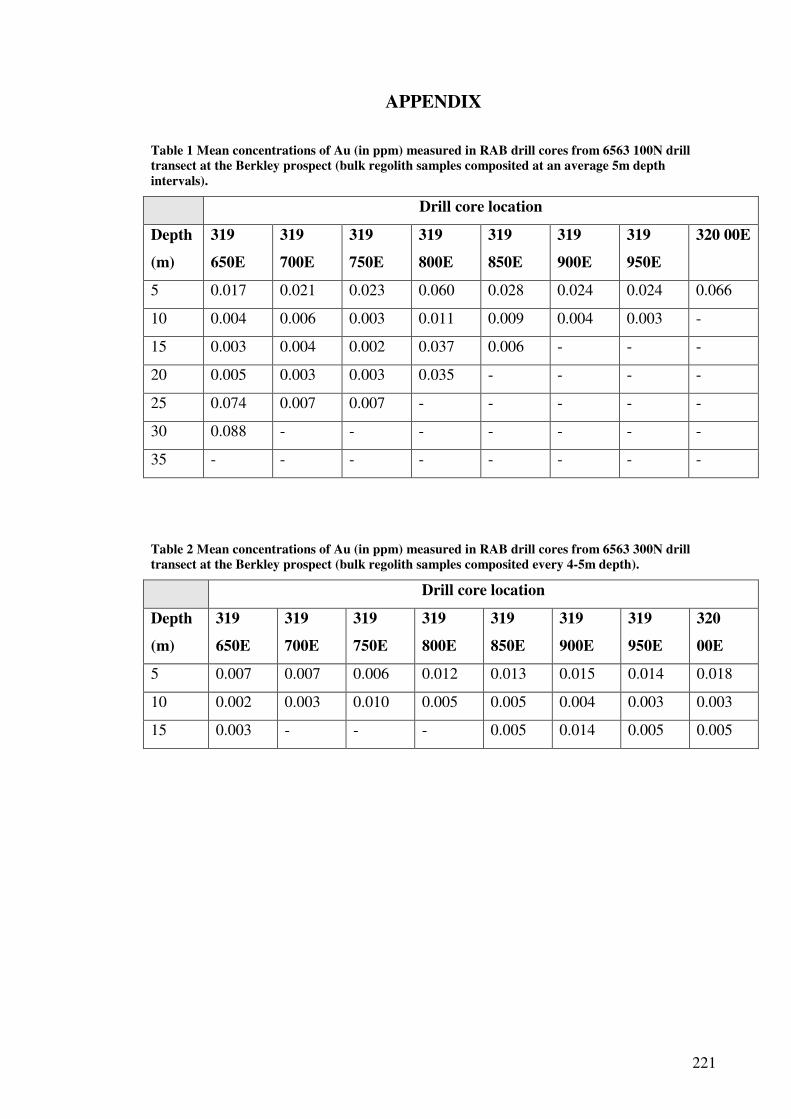
221

APPENDIX

Table 1 Mean concentrations of Au (in ppm) measured in RAB drill cores from 6563 100N drill

transect at the Berkley prospect (bulk regolith samples composited at an average 5m depth

intervals).

Drill core location

Depth

(m)

319

650E

319

700E

319

750E

319

800E

319

850E

319

900E

319

950E

320 00E

5 0.017 0.021 0.023 0.060 0.028 0.024 0.024 0.066

10 0.004 0.006 0.003 0.011 0.009 0.004 0.003 -

15 0.003 0.004 0.002 0.037 0.006 - - -

20 0.005 0.003 0.003 0.035 - - - -

25 0.074 0.007 0.007 - - - - -

30 0.088 - - - - - - -

35 - - - - - - - -

Table 2 Mean concentrations of Au (in ppm) measured in RAB drill cores from 6563 300N drill

transect at the Berkley prospect (bulk regolith samples composited every 4-5m depth).

Drill core location

Depth

(m)

319

650E

319

700E

319

750E

319

800E

319

850E

319

900E

319

950E

320

00E

5 0.007 0.007 0.006 0.012 0.013 0.015 0.014 0.018

10 0.002 0.003 0.010 0.005 0.005 0.004 0.003 0.003

15 0.003 - - - 0.005 0.014 0.005 0.005

Documents

Vegetation as a biotic driver for the formation of soil geochemical ...€¦ · anomalies for mineral exploration of covered terranes Soil is a relatively low cost and robust geochemical