Embed Size (px)
Citation preview

VECTORS
David J. Jeffery1
2008 January 1
ABSTRACT
Lecture notes on what the title says and what the subject headings say.
Subject headings: scalars — vectors — trigonometry — Cartesian coordinates
— trigonometric functions — trigonometric identities — vector components —
vector math — vector addition — vector multiplication by scalars — unit vectors
— vector math — dot product
1. INTRODUCTION
How many people are already familiar with scalars and vectors? Show of hands.
Some, many, few?
For those folks, this lecture may be mainly review, but perhaps at an interesting level.
One thing to say at the start is we are NOT going to deal with scalars and vectors in a
rigorous math sense. We leave that to a course in linear algebra. Actually, even in physics, a
more formal definition of a vector is needed in more advanced work that involves specifying
the transformation properties of vectors, but we don’t need that.
1 Department of Physics, University of Idaho, PO Box 440903, Moscow, Idaho 83844-0903, U.S.A. Lecture
posted as a pdf file at http://www.nhn.ou.edu/~jeffery/course/c intro/introl/003 vec.pdf .

– 2 –
In physics properly speaking, scalars are quantities (or entities) that are expressed by
a single real number (that can be positive, negative, or zero) that is independent of the
coordinate system used to describe ordinary physical space—or space space as yours truly
likes to call it. Note integers, rational, and irrational numbers are all subsets of real numbers.
Examples of scalars are temperature, density, pressure.
In math on the other hand, scalars are just real numbers in the context of linear algebra.
In fact, in physics, the word scalar is used in non-rigorous communication to mean either
a physical scalar (e.g., temperature, density, pressure) or a real number. For example, we
can call the components of a vector scalars since they are real numbers, but arn’t physical
scalars and we can talk of scalar addition meaning real number addition. Context decides
which kind of scalar we mean.
In physics, vectors are quantities (or entities) that are expressed by a magnitude (a
positive or zero number) and a direction in space space. The magnitude and direction of the
independent of the coordinate system.
Examples, we have already discussed in the lecture ONE-DIMENSIONAL KINEMAT-
ICS are displacement, velocity, and acceleration.
Physical vectors usually have dimensions and units. For example, displacement has
dimensions of length and the MKS unit the meter.
To represent a vector, one usually uses a letter with an arrow above it. For example,
consider general vector ~A. The magnitude of ~A can be written | ~A|. But, in fact, very
commonly and throughout these lectures, we represent the magnitude of a vector by using
the vector symbol without the arrow. Thus, A is the magnitude of ~A. In cursive script, a
vector can be represented by a letter with a squiggle beneath it. Yours truly uses this form
all the time when writing cursively—get used to it.

– 3 –
Many vector quantities in physics have common symbols. For example, common symbols
for displacement, velocity, and acceleration are, respectively, ~r, ~v, and ~a. But common
symbols are not always used. Some authors have different traditions. Sometimes other
symbols are needed to prevent confusion for some reason.
A key point about vectors is that their magnitude is frequently called their length.
But this length is only an extension in space space for displacement. All other vectors
have their extension in an abstract vector space of their own particular class. Velocities
vectors are extended in velocity space, acceleration vectors are extended in acceleration
space, et cetera.
But to reiterate, vector direction is in space space. If a vector has zero magnitude, then
its direction in space space is indefinite.
Many physical quantities of great interest are vectors. The aforesaid, displacement,
velocity, and acceleration. But many other quantities, we encounter in intro physics: e.g.,
force, momentum, angular momentum, torque, the gravitational field, electric field, and
magnetic field to name just the most prominent.
So we have to deal with vectors in intro physics.
In principle, they are not hard to deal with at our level.
But, also at our level, it’s often tedious to do calculations with them.
We just have to bite the bullet and do those calculations
VECTORS can be one-, two-, three-, or higher-dimensional. The higher-dimensional
vectors won’t turn up in our course and we’ll mostly deal in calculations with only one- and
two-dimensional vectors.
We have already worked in with one-dimensional vectors in the lecture ONE-DIMENSIONAL

– 4 –
KINEMATICS. But they are really easy to work with since they have only two directions.
Thus, one usually omits formal vector notation and specifies direction by sign: positive for
one direction and negative for the other direction. Sometimes three-dimensional vectors turn
up in intro physics. We’ll consider three-dimensional vectors briefly in § 6.
Now as mentioned above, scalars and vectors are independent of coordinate systems.
This must be so.
Coordinate systems are arbitrary descriptions of space used to describe physical systems.
So physical quantities should not depend on the descriptions.
But the description of the physical quantity can depend on them.
For vectors, the most efficient description is often to use vector components rather than
magnitude and direction. We’ll go into vector components in § 4.
The vector components ARE dependent on the coordinate system unlike magnitude
and direction. This is drawback of vector components. But as aforesaid, they are often the
most efficient description.
The reason is that vector calculations are often straightforward using vector components.
Often vector components don’t give a great intuitive sense of the vector quantity’s effect
in a system unlike magnitude and direction. So usually in intro physics problems give input
values for vectors in terms of magnitude and direction. For solution, one finds the vector
components in a particular coordinate system and then solves using the components. The
output value components are often then converted into magnitude and direction format to
report the solution.
The coordinate system used for the problem can often be chosen to make the problem
easier to solve. Very often, one can choose a coordinate system where a coordinate axis aligns
– 5 –
with one or more vectors. Doing this simplifies the determination of the vector components.
To deal with vector components, we need trigonometry.
2. TRIGONOMETRY
The word trigonometry is derived from Greek words meaning triangle and measurement.
Originally it was confined to the study of the relationships of the sides and angles of
triangles.
But trigonometry is nowadays extended beyond triangles to deal with negative lengths.
This extension is essential for the treatment of vector components.
So we don’t bother to start just with the triangle case.
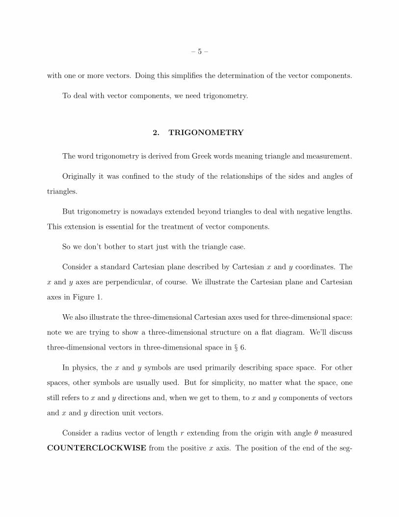
Consider a standard Cartesian plane described by Cartesian x and y coordinates. The
x and y axes are perpendicular, of course. We illustrate the Cartesian plane and Cartesian
axes in Figure 1.
We also illustrate the three-dimensional Cartesian axes used for three-dimensional space:
note we are trying to show a three-dimensional structure on a flat diagram. We’ll discuss
three-dimensional vectors in three-dimensional space in § 6.
In physics, the x and y symbols are used primarily describing space space. For other
spaces, other symbols are usually used. But for simplicity, no matter what the space, one
still refers to x and y directions and, when we get to them, to x and y components of vectors
and x and y direction unit vectors.
Consider a radius vector of length r extending from the origin with angle θ measured
COUNTERCLOCKWISE from the positive x axis. The position of the end of the seg-

– 6 –
ment is the ordered pair (x, y).
The measurement of θ COUNTERCLOCKWISE from the positive x axis is conven-
tional. We usually conform to the convention which is the convention of polar coordinates.
The convention is occasionally dropped for special cases, but it is pretty usual in physics
and math.
Actually, θ as we have defined it is the angular polar coordinates for polar coordinates.
The symbol θ is the small Greek letter theta. Besides being the angle of polar coordinates
and the polar angle of spherical polar coordinates (see § 6), θ is the usual first choice for the
symbol for any angle in physics. But other symbols must be used too since one can have
more than one angle in a system. Two angles are needed for spherical polar coordinates for
example, and so there are two conventional angle symbols θ and φ (see § 6). Alternatively,
for more than one angle one can use θ with appropriate subscripts. Either way or both.
We note that the projection of the radius vector onto the x axis has length x. Similarly
the projection of the radius vector onto the y axis has length y.
In Figure 1, we put the radius in the 1st quadrant, but that is just for example. The
radius could be in any quadrant of the plane. The quadrants are usually counted going
Fig. 1.— Two- and three-dimensional Cartesian coordinates with a radius vector.
– 7 –
counterclockwise and starting from the positive x axis.
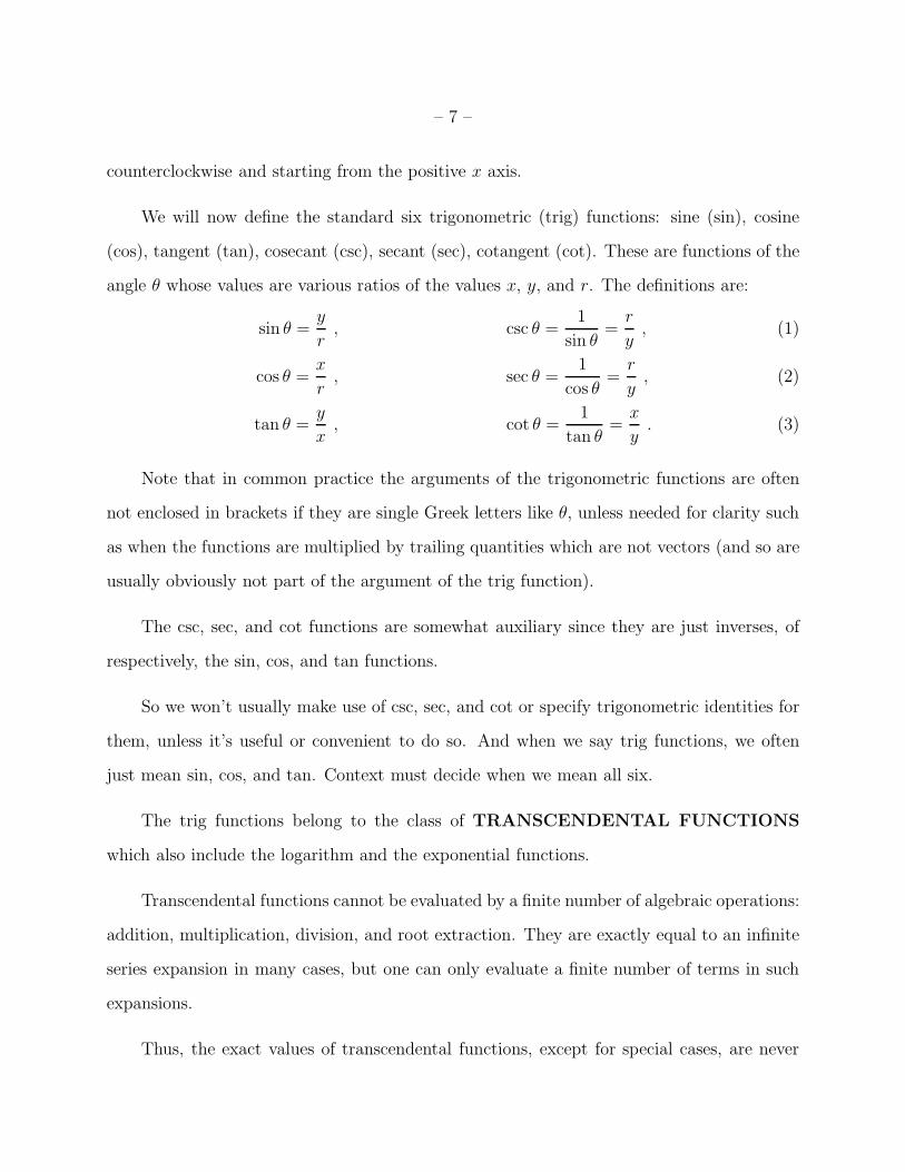
We will now define the standard six trigonometric (trig) functions: sine (sin), cosine
(cos), tangent (tan), cosecant (csc), secant (sec), cotangent (cot). These are functions of the
angle θ whose values are various ratios of the values x, y, and r. The definitions are:
sin θ =y
r, csc θ =
1
sin θ=
r
y, (1)
cos θ =x
r, sec θ =
1
cos θ=
r
y, (2)
tan θ =y
x, cot θ =
1
tan θ=
x
y. (3)
Note that in common practice the arguments of the trigonometric functions are often
not enclosed in brackets if they are single Greek letters like θ, unless needed for clarity such
as when the functions are multiplied by trailing quantities which are not vectors (and so are
usually obviously not part of the argument of the trig function).
The csc, sec, and cot functions are somewhat auxiliary since they are just inverses, of
respectively, the sin, cos, and tan functions.
So we won’t usually make use of csc, sec, and cot or specify trigonometric identities for
them, unless it’s useful or convenient to do so. And when we say trig functions, we often
just mean sin, cos, and tan. Context must decide when we mean all six.
The trig functions belong to the class of TRANSCENDENTAL FUNCTIONS
which also include the logarithm and the exponential functions.
Transcendental functions cannot be evaluated by a finite number of algebraic operations:
addition, multiplication, division, and root extraction. They are exactly equal to an infinite
series expansion in many cases, but one can only evaluate a finite number of terms in such
expansions.
Thus, the exact values of transcendental functions, except for special cases, are never

– 8 –
known by a finite numeral expression. However, one can always evaluate them to whatever
precision you like by evaluating more terms in the series expansion if there is one. The
series expansions for sin, cos, and, for the first 4 terms, for tan are given in Table 1 for
completeness. Computers and calculators typically use some sort of expansion to evaluate
transcendental functions to high, but finite, precision.
As well as using series expansions, which we won’t go into here, one can also evaluate
trig functions geometrically by measuring lengths. But our calculators obviate the need for
that.
Since the trig functions can be evaluated by a series expansions, their arguments do
not have to be geometrical angles and their values do not have to be interpreted as ratios
of lengths. In fact, the trig functions do turn up in many non-geometrical contexts in math
and physics. One those contexts is describing the motion of the simple harmonic oscillator
which we get to in the lecture NEWTONIAN PHYSICS II.
If one confines θ to the 1st quadrant (i.e., confines θ to the range [0◦, 90◦]), then the trig
functions are the unextended trig functions for a triangle. The radius r is the hypotenuse of
a right triangle (i.e., a right-angled triangle) with sides of length x and y. For angle θ, the x
side is called the adjacent and the y side is called the opposite. For angle at the radius head
(the complementary angle to angle θ), the x side is the opposite and and the y side is the
adjacent.
One can now give the familiar unextended word definitions of sin as opposite over
hypotenuse, cos as adjacent over hypotenuse, and tan as opposite over adjacent. These
definitions don’t require specifying a coordinate system.
The first thing to note about the trig functions is that they do not depend on the
absolute lengths of the line segments, but only on ratios. This makes the trig functions of

– 9 –
great general utility in math and physics since absolute size of lengths is not relevant in the
evaluation of the trig functions.
The second thing to note is the relationship between sin, cos, and tan.
What is tan θ equal to in terms of sin θ and cos θ?
You have 30 seconds. Go
Well
tan θ =y
x=
y/r
x/r=
sin θ
cos θ, (4)
whence
tan θ =sin θ
cos θ. (5)
A third thing to note is the evenness/oddness of the trig functions. We see that
sin(−θ) =−y
r= − sin(θ) , (6)
cos(−θ) =x
r= cos(θ) , (7)
tan(−θ) =sin(−θ)
cos(−θ)=
− sin(θ)
cos(θ)= − tan θ , (8)
whence
sin(−θ) = − sin(θ) , cos(−θ) = cos(θ) , tan(−θ) = − tan θ . (9)
We see that sin and tan are odd functions of their arguments and cos is an even function of
its argument.
The third thing to notice about the trig functions is that they are periodic. Their values
repeat every time the argument θ increases by 360◦. In Figure 2, we show the plots of the
trig functions.
The plots in Figure 2 show the periodic behavior. They also show that sin and cos values
are limited to the range [−1, 1]. The tan function has an infinite discontinuity whenever

– 10 –
θ = 90◦ + 180◦n, where n is a general integer. This is actually clear from the tan definition
equation (3) since at these angles one has a division by x = 0 and tangent function value
changes sign x goes from negative to positive as θ goes increases through the point of infinite
discontinuity.
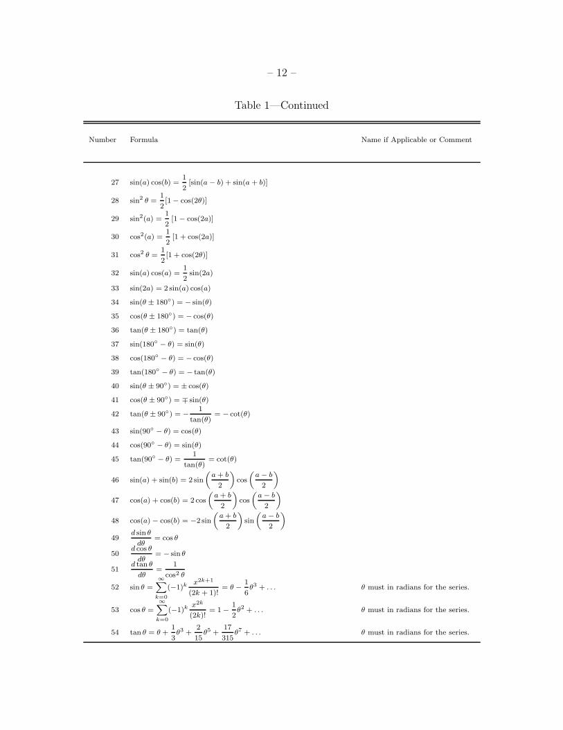
For the sake of general reference Table 1 gives a large, but not exhaustive, list of trigono-
metric formulae which include the trig function definitions, special trig function values, trig
identities, derivatives of trig functions, and trig function series expansions.
The formulae are roughly in order of utility in the opinion of yours truly. The formulae
1 to 22 are most important for this lecture in yours truly’s opinion thinks. You should
memorize these formulae.
Fig. 2.— Plots of trig functions sin θ, cos θ, and tan θ.

– 11 –
Table 1. Trigonometric Formulae
Number Formula Name if Applicable or Comment
1 sin θ =y
rsine function
2 cos θ =x
rcosine function
3 tan θ =y
xtangent function
4 csc θ =1
sin θ=
r
ycosecant function
5 sec θ =1
cos θ=
r
xsecant function
6 cot θ =1
tan θ=
x
ycotangent function
7 tan θ =sin θ
cos θ
8 f(θ) = f(θ + 360◦) f is any trigonometric function.
9 c2 = a2 + b2 Pythagorean theorem
10 cos2 θ + sin2 θ = 1
11 c2 = a2 + b2 − 2ab cos θc law of cosines
12sin θa
a=
sin θb
b=
sin θc
claw of sines
13 sin(0◦) = 0 cos(0◦) = 1 tan(0◦) = 0
14 sin(90◦) = 1 cos(90◦) = 0 tan(90◦) = ∞
15 sin(45◦) =1√2
= 0.7071 . . . cos(45◦) =1√2
= 0.7071 . . .
tan(45◦) = 1
16 cos(30◦) =
√3
2= 0.8660 . . . sin(30◦) =
1
2
tan(30◦) =1√3
= 0.57735 . . .
17 cos(60◦) =1
2sin(60◦) =
√3
2= 0.8660 . . .
tan(60◦) =√
3 = 1.73205 . . .
18 sin(−θ) = − sin(θ)
19 cos(−θ) = cos(θ)
20 tan(−θ) = − tan(θ)
21 sin(a + b) = sin(a) cos(b) + cos(a) sin(b)
22 cos(a + b) = cos(a) cos(b) − sin(a) sin(b)
23 sin(2a) = 2 sin(a) cos(a)
24 cos(2a) = cos2(a) − sin2(a)
25 sin(a) sin(b) =1
2[cos(a − b) − cos(a + b)]
26 cos(a) cos(b) =1
2[cos(a − b) + cos(a + b)]
– 12 –
Table 1—Continued
Number Formula Name if Applicable or Comment
27 sin(a) cos(b) =1
2[sin(a − b) + sin(a + b)]
28 sin2 θ =1
2[1 − cos(2θ)]
29 sin2(a) =1
2[1 − cos(2a)]
30 cos2(a) =1
2[1 + cos(2a)]
31 cos2 θ =1
2[1 + cos(2θ)]
32 sin(a) cos(a) =1
2sin(2a)
33 sin(2a) = 2 sin(a) cos(a)
34 sin(θ ± 180◦) = − sin(θ)
35 cos(θ ± 180◦) = − cos(θ)
36 tan(θ ± 180◦) = tan(θ)
37 sin(180◦ − θ) = sin(θ)
38 cos(180◦ − θ) = − cos(θ)
39 tan(180◦ − θ) = − tan(θ)
40 sin(θ ± 90◦) = ± cos(θ)
41 cos(θ ± 90◦) = ∓ sin(θ)
42 tan(θ ± 90◦) = − 1
tan(θ)= − cot(θ)
43 sin(90◦ − θ) = cos(θ)
44 cos(90◦ − θ) = sin(θ)
45 tan(90◦ − θ) =1
tan(θ)= cot(θ)
46 sin(a) + sin(b) = 2 sin
„
a + b
2
«
cos
„
a − b
2
«
47 cos(a) + cos(b) = 2 cos
„
a + b
2
«
cos
„
a − b
2
«
48 cos(a) − cos(b) = −2 sin
„
a + b
2
«
sin
„
a − b
2
«
49d sin θ
dθ= cos θ
50d cos θ
dθ= − sin θ
51d tan θ
dθ=
1
cos2 θ
52 sin θ =∞
X
k=0
(−1)kx2k+1
(2k + 1)!= θ − 1
6θ3 + . . . θ must in radians for the series.
53 cos θ =∞
X
k=0
(−1)kx2k
(2k)!= 1 −
1
2θ2 + . . . θ must in radians for the series.
54 tan θ = θ +1
3θ3 +
2
15θ5 +
17
315θ7 + . . . θ must in radians for the series.

– 13 –
Note. — The trigonometric functions are definitions. The other formulae are standard special trig function values,
trig identities, trig function derivatives, and trig function series expansions. The variables a, b, c are general; θ is a
general angle; x and y are the projections of the general radius r on the x axis and y axis, respectively. In the laws
of cosines and sines, θa, θb and θc respectively, subtend the sides of lengths a, b, and c. Our list is not meant to be
exhaustive. The formulae are listed in roughly in order of utility in the opinion of yours truly. The formulae 1 to
22 are most important for this lecture in yours truly’s opinion thinks. General references are the Wikipedia articles
Trigonometric function (http://en.wikipedia.org/wiki/Trigonometric functions) and List of trigonometric identities
(http://en.wikipedia.org/wiki/List of trigonometric identities).

– 14 –
We have already proven some important trig identities above and we prove a few more
in the following subsections. After we have developed some more formalism, we will prove
some other important trig identities § 8. Many other trig identities follow as special cases
of the more important ones. To show how this is done, we derive a few more identities in
Appendix A. We do NOT prove all identities and formulae that appear in Table 1, but we
do prove a lot of them.
We will show in following subsections how to evaluate the trig functions exactly for
certain standard special argument values to obtain the standard special trig function values.
First though we’ll give the simplest proof yours truly knows for the Pythagorean theorem
since it’s good to know the proof and we’ll need the theorem in this lecture and throughout
the course.
2.1. Proof of the Pythagorean Theorem
To prove the Pythagorean theorem, first consider the big square and the inscribed
smaller square in Figure 3.
The inscribed square is angled obliquely relative to the big square and its vertices touch
Fig. 3.— Square and inscribed square for proving the Pythagorean theorem.
– 15 –
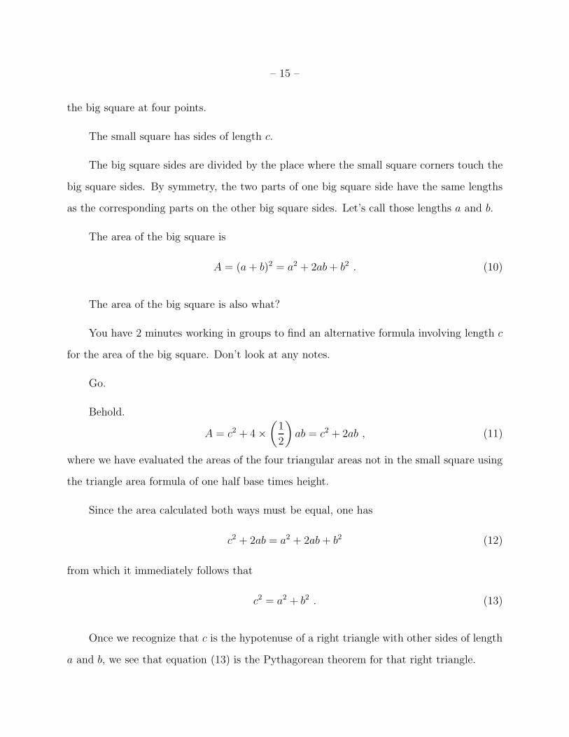
the big square at four points.
The small square has sides of length c.
The big square sides are divided by the place where the small square corners touch the
big square sides. By symmetry, the two parts of one big square side have the same lengths
as the corresponding parts on the other big square sides. Let’s call those lengths a and b.
The area of the big square is
A = (a + b)2 = a2 + 2ab + b2 . (10)
The area of the big square is also what?
You have 2 minutes working in groups to find an alternative formula involving length c
for the area of the big square. Don’t look at any notes.
Go.
Behold.
A = c2 + 4 ×(
1
2
)
ab = c2 + 2ab , (11)
where we have evaluated the areas of the four triangular areas not in the small square using
the triangle area formula of one half base times height.
Since the area calculated both ways must be equal, one has
c2 + 2ab = a2 + 2ab + b2 (12)
from which it immediately follows that
c2 = a2 + b2 . (13)
Once we recognize that c is the hypotenuse of a right triangle with other sides of length
a and b, we see that equation (13) is the Pythagorean theorem for that right triangle.

– 16 –
Since our big and small square is general, the lengths a and b have can have any values.
Thus, the equation (13) applies to any right triangle and we have a general proof of the
Pythagorean theorem.
A real rigorous geometrical proof of the Pythagorean theorem would probably take full
account of a lot of concepts implicit in our proof. For example the concept of area that we
use without discussion. But “Sufficient unto the day is the rigor thereof.”
Note that for the construction that we used to introduce the trigonometric functions
that
r2 = x2 + y2 (14)
by the Pythagorean theorem since r, |x|, and |y form the sides of a triangle. It follows then
that
r2 = r2 cos2 θ + r2 sin2 θ (15)
or
1 = cos2 θ + sin2 θ (16)
which is an important trigonometric identity appearing in Table 1
2.2. Trig Function Values for θ = 0◦ and θ = 180◦
From the trig function definitions, the trig functions evaluated for θ = 0◦ and θ = 180◦
are, respectively,
sin(0◦) = 0 , cos(0◦) = 1 , tan(0◦) = 0 (17)
and
sin(180◦) = 0 , cos(180◦) = −1 , tan(180◦) = 0 . (18)

– 17 –
In these cases, the triangles formed by the line segments have been collapsed to line
segments.
2.3. Trig Function Values for θ = 90◦ and θ = 270◦
From the trig function definitions, the trig functions evaluated for θ = 90◦ and θ = 270◦
are, respectively,
sin(90◦) = 1 , cos(90◦) = 0 , tan(90◦) = ∞ (19)
and
sin(270◦) = −1 , cos(270◦) = 0 , tan(90◦) = −∞ (20)
In these cases, the triangles formed by the line segments have been collapsed to line
segments.
2.4. Trig Function Values for θ = 45◦
If θ = 45◦, then the other non-right angle in the right triangle formed by the line
segments is must be θ = 45◦ by the rule (which we won’t prove) that the sides of triangle
add up to 180◦.
By the isosceles triangle theorem, y = x. Thus, from the Pythagorean theorem
r2 = x2 + y2 = 2x2 . (21)
From the trig function definitions, the trig functions evaluated for θ = 45◦ are
sin(45◦) =y√2x
=x√2x
=1√2
= 0.7071 . . . , (22)

– 18 –
cos(45◦) =x√2x
=1√2
= 0.7071 . . . , (23)
tan(45◦) = 1 . (24)
2.5. Trig Function Values for θ = 30◦ and θ = 60◦
Evaluating the trig functions for θ = 30◦ and θ = 60◦ is a little trickier than the earlier
cases.
It’s not something most people can think of off the top of their heads.
Consider a regular hexagon (as illustrated in Fig. 4) divided into 6 triangles by lines
connecting opposing vertices. The lines must all intersect at the geometric center of the
hexagon. By symmetry, the triangles must all be similar and all be isosceles triangles. They
must all have angles 60◦ at the geometric center of the hexagon since these angles must add
up to 360◦.
Consider one triangle. Since it is isosceles, the non-center angles must be equal and
since all the angles must add up to 180◦, all the angles of the triangle are 60◦. Thus, all
the sides of the triangle are equal since the triangle is isosceles relative to any vertex. Let
the side length be c. Bisect angle of the triangle that is at the center of the hexagon by a
perpendicular to the opposing side.
Consider one of the triangles formed by the bisection. It is a right triangle with angles
30◦, 60◦, and, of course, 90◦. The side opposing the 30◦ angle has length c/2. Using the
Pythagorean theorem, it follows that the side opposing the 60◦ angle and adjacent to the
30◦ angle has length√
c2 −( c
2
)2
= c
√3
2. (25)
– 19 –
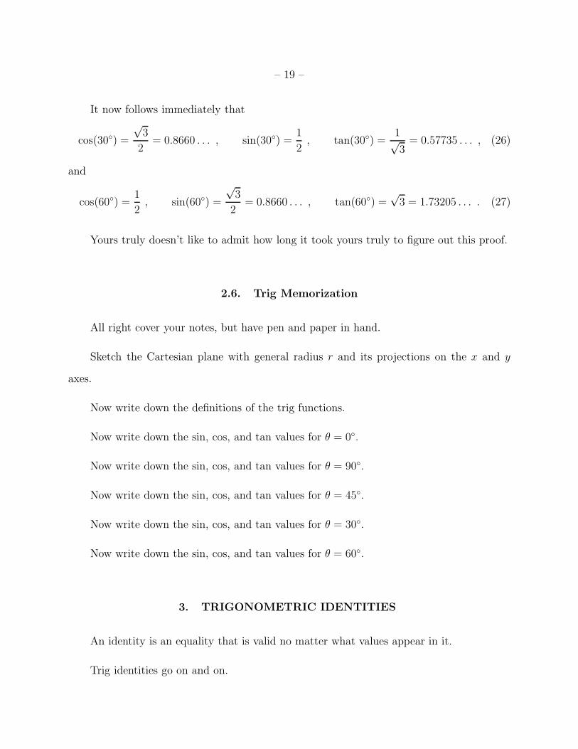
It now follows immediately that
cos(30◦) =
√3
2= 0.8660 . . . , sin(30◦) =
1
2, tan(30◦) =
1√3
= 0.57735 . . . , (26)
and
cos(60◦) =1
2, sin(60◦) =
√3
2= 0.8660 . . . , tan(60◦) =
√3 = 1.73205 . . . . (27)
Yours truly doesn’t like to admit how long it took yours truly to figure out this proof.
2.6. Trig Memorization
All right cover your notes, but have pen and paper in hand.
Sketch the Cartesian plane with general radius r and its projections on the x and y
axes.
Now write down the definitions of the trig functions.
Now write down the sin, cos, and tan values for θ = 0◦.
Now write down the sin, cos, and tan values for θ = 90◦.
Now write down the sin, cos, and tan values for θ = 45◦.
Now write down the sin, cos, and tan values for θ = 30◦.
Now write down the sin, cos, and tan values for θ = 60◦.
3. TRIGONOMETRIC IDENTITIES
An identity is an equality that is valid no matter what values appear in it.
Trig identities go on and on.

– 20 –
Some are memorable and used a lot.
Others turn up more rarely.
In the following subsections we give and prove some common trig identities.
4. VECTOR COMPONENTS
The component of a vector for a coordinate direction is the magnitude of the vector
times the cosine of the angle the vector makes with the coordinate direction.
A vector is fully specified, in fact, by the set of components it has for all the coordinate
directions of a coordinate system that describes the space in which the vector is embedded.
We will verify this below for two-dimensional vectors using Cartesian coordinates.
Usually we will deal with vectors in two-dimensional and three-dimensional space and
use Cartesian coordinates.
In this section, we will just deal with two-dimensional vectors and leave three-dimensional
vectors to § 6.
Cartesian coordinates are conceptually the easiest to deal with at first glance. This
is because the Cartesian coordinate directions are global. This means that every point in
space the coordinate directions: e.g., the x direction at one point is the same as at another.
Curvilinear coordinates such as polar coordinates (used for two dimensions) or spherical polar
coordinates (AKA spherical coordinates and used for three dimensions) trickier because the
coordinate directions are local: i.e., they vary with position. For example the radial direction
in polar coordinates for a point in space depends on the angle of the radius vector to that
point.
Why deal with curvilinear coordinates? Well sometimes to exploit the symmetry of a

– 21 –
system, curvilinear coordinates offer the obvious approach. A circularly symmetric system
about some central in two-dimensional space is often best treated by using polar coordinates
with the origin at the central point.
In actual fact, one frequently has to use both Cartesian and curvilinear coordinates for
systems. One flips back and forth as needs be. We’ll be doing that in this section and this
lecture. Just get used to flipping.
Say ~A is a general two-dimensional vector in a general two-dimensional space which we
describe by Cartesian axes. Unless the vector is displacement, the space is not space space,
but an abstract space like velocity space and acceleration space.
The tail of the vector is always located at the origin of the space and its head is located
at some point in the space. The vector points from tail to head.
For physical vectors, the directions of the abstract space correspond to the directions of
space space. Therefore for two dimensions, we just say x direction, y direction, x axis, y axis
et cetera no matter what abstract space is being considered Similarly for three dimensions,
we just say x direction, y direction, z direction, et cetera no matter what abstract space is
being considered.
The x and y components of ~A with the Cartesian axes are, respectively,
Ax = A cos θ and Ay = A cos θy (28)
where θ without subscript is the angle of between the vector and the x axis and θy is the
angle of between the vector and the y axis.
The geometrical interpretation of a component follows from the definition of cosine. It
is the projection of the vector ~A along the axis for the component. The projection is made
looking perpendicularly at the axis.
– 22 –
Following the convention of polar coordinates, θ is measured counterclockwise from the
positive x axis. The sign of θ actually has no effect on the component value since cosine is an
even function of θ. So one could decide that θ should be positive no matter what orientation
the vector has relative to the x axis. But following the convention of polar coordinates
simplifies the discussion, in particular, for θy which we want to relate to θ.
The angle θ is, in fact, the coordinate angle of polar coordinates. The radial component
of polar coordinates for ~A is just the magnitude A. Note we are already flipping between
Cartesian and polar coordinates.
Similarly, we choose to measure θy counterclockwise positive y axis. Thus, we have
θy = θ − 90◦ . (29)
Note that if the ~A points into the 1st quadrant of the Cartesian plane θy is negative.
Thus,
cos θy = cos(θ − 90◦) = cos θ cos(90◦) + sin θ sin(90◦) = sin θ , (30)
where we have used a trig identity from Table 1.
Therefore, the x and y components of ~A with the Cartesian axes can be written, respec-
tively,
Ax = A cos θ , (31)
Ay = A sin θ (32)
which is the usual way to write the components of two-dimensional vectors.
A vector is fully specified by its magnitude and direction. In principle, you don’t need
any coordinate system to specify magnitude and direction. But you have to specify direction
relative to something like physical objects. So why not an angle relative to a coordinate
direction? In two dimensions, you actually need one angle (which is θ in polar coordinates)

– 23 –
to specify the direction relative to some axis. In three dimensions, you need two angles
relative to two axes to specify the direction as we show in § 6.
The vector components as mentioned above also fully specify a vector.
We now show explicitly how to specify the vector fully from Cartesian components for
two-dimensions by showing that magnitude and direction can be obtained from the Cartesian
components.
The magnitude is simple to obtain from the components. We find
√
A2x + A2
y =√
A2 cos2 θ + A2 sin2 θ = A√
cos2 θ + sin2 θ = A , (33)
where we have used a trig identity from Table 1.
Direction is fully specified by θ, in fact. We note that
Ay
Ax
=A sin θ
A cos θ= tan θ , (34)
and so
θ =
tan−1
(
Ay
Ax
)
for Ax > 0;
tan−1
(
Ay
Ax
)
+ 180◦ for Ax < 0;
90◦ for Ax = 0 and Ay > 0;
−90◦ for Ax = 0 and Ay < 0;
undefined for Ax = Ay = 0,
(35)
where tan−1 is the inverse tangent function.
The need for the additive term 180◦ in the above specification is because the inverse
tangent function is defective for recovering the angle for from a tangent value. This because
tangent value for angles in the range [−180◦, 180◦] is mapped to by two angles: a first angle
in the range [−90◦, 90◦] and a second angle from outside the range [−90◦, 90◦] that differs
by 180◦ from the first angle. In defining the inverse tangent function, it was decided that
– 24 –
it should map a value to the angle in the range [−90◦, 90◦]. All calculator and computer
inverse tangent functions adhere to this convention. But if the x component for a vector is
negative, you know that the vector angle is really in not in the range [−90◦, 90◦] but is 180◦
degrees away from the value the inverse tangent function gives. It’s a nuisance to always
have to worry about adding or not adding 180◦ to an inverse tangent function result, but
that’s the way it is.
Another way to to look at this inverse tangent function defect is to say that the inverse
tangent function has no way to know the sign of the components in the ratio Ay/Ax, and so
by convention always assumes Ax > 0. For example if Ay/Ax is positive, the inverse tangent
function cannot actually know if both components are positive or both are negative. It
assumes Ax > 0 by the convention and this implies Ay is positive and the vector points into
the 1st quadrant. But if both components are actually negative, then the vector actually
points 180◦ away into the 3rd quadrant.
To summarize, the formulae for finding magnitude and direction of a general two-
dimensional vector from its Cartesian components are
A =√
A2x + A2
y (36)
θ = tan−1
(
Ay
Ax
)
+ 180◦n . (37)
Since A is fully specified by its components, one can represent the vector by an ordered
pair of its components. For Cartesian components, we can write
~A = (Ax, Ay) . (38)
For Cartesian coordinates, the components are coordinates of the point located by the
vector. This is not the case for curvilinear components.
– 25 –
For example, in polar coordinates, we can write the ordered-pair form
~A = (A, θ) , (39)
where A and θ are the polar coordinates of the point in the space of vector ~A located by
~A. But absolutely positively A and θ are NOT vector components as we have defined
them. They are just polar coordinates. If one wants to express a vector in polar coordinate
components, one usually introduces polar coordinate unit vectors. We do this in § 5.8.
Let’s special to the displacement vector ~r. For Cartesian coordinates
~r = (x, y) , (40)
where x and y are components for ~r and are the coordinates for the point located by ~r. For
polar coordinates,
~r = (r, θ) , (41)
where again r and θ are not vector components as we have defined them, but only the polar
coordinates of point located by ~r.
Absolutely, positively, the components of a vector are not unique. They are dependent
on the coordinate system they are determined for. The components always determine the
vector’s magnitude and direction though.
Both because magnitude and direction give a concrete sense of what a vector does in
physics and because magnitude and direction are unique and not dependent on arbitrary
choices of coordinate systems, people often prefer to think in terms of magnitude and direc-
tion as specifying a vector. Thus, problems involving vectors are often set giving magnitude
and direction and require magnitude and direction in answers.
Why do we need vector components then?

– 26 –
First for calculations, where vector components are usually the only efficient way to do
the calculations.
But second and equally importantly for conceptual work for many purposes. For ex-
ample, for the proofs we do in § 5 just below on vector math. In tensor math, which is
generalization of vector math, component formalism is also needed for many purposes. But
one does have to say that there is a component-free approach to tensor math (see Wikipedia:
Tensor (intrinsic definition)) of which yours truly knows little.
5. VECTOR MATH
We need some vector math.
This vector math is correct for physically defined vectors and that is its justification.
All our proofs and illustrations are for two-dimensional vectors for simplicity.
But all the proofs and illustrations obviously generalize to multi-dimensional vectors in
multi-dimensional Euclidean space.
5.1. Vector Addition
We know how to add real numbers, but how does one add vectors?
Vector addition has to be defined actually.
Yours truly thinks it best to just define vector addition in terms of vector components
which are real numbers.
Say ~A and ~B are general vectors. If they are actually physical vectors, they must be
of the same type: e.g., displacement vectors or velocity vectors. It just turns out in physics

– 27 –
that the vectors must be of the same type for the sum to have any physical meaning.
In component form one has
~A = (Ax, Ay) and ~B = (Bx, By) (42)
We define the sum of the vectors to by
~A + ~B = (Ax + Bx, Ay + By) . (43)
We add the components for each coordinate direction by real number addition.
The vector addition rule has simple geometrical interpretation.
One takes vector ~B and mentally transports its tail from the origin to the head of vector
~A without changing its direction. There is now a vector that stretches from the origin to
the head of the transplanted ~B. This new vector is exactly vector obtained by the vector
addition rule
This geometrical interpretation is so obvious that it almost defies further explication.
But if you think about where Ax + Bx and Ay + By put the tip of the vector sum, then
maybe that helps.
Figure 5 shows illustrates the geometrical interpretation.
One can use the geometrical interpretation to add vectors by geometrical means if one
chooses. For qualitative thinking about or illustration of vector sums this is often very useful.
For quantitative calculations it is not usually useful.
5.2. Vector Multiplication by A Real Number
Vector multiplication by a real number must also be defined.

– 28 –
Fig. 4.— A regular hexagon from which the special trig function values for angles 30◦ and
60◦ can be deduced.
Fig. 5.— Vector addition in the geometric interpretation.

– 29 –
There is no way that it can just be deduced from our definition of vectors and the
properties of real numbers.
But the definition is the obvious one.
Say ~A is a general vector and c is a general real number.
We define
c ~A = (cAx, cAy) , (44)
where cAx and cAy are just ordinary real number multiplications.
5.3. The Inverse of a Vector and the Zero Vector
The definition of an inverse of ~A which we represent by − ~A is then the obvious one:
− ~A = (−Ax,−Ay) . (45)
With this definition
~A + (− ~A) = (Ax − Ax, Ay − Ay) = (0, 0) . (46)
The vector (0, 0) is the zero or null vector. The zero vector has zero magnitude and an
undefined direction.
Actually, the zero vector is usually represented by 0. No arrow sign over the zero is used
by convention.
The inverse of vector has the same magnitude of the vector obviously.
Almost as obviously it points in the opposite direction.
To be definite we see immediately that the magnitude of − ~A is given by
| − ~A| =√
(−Ax)2 + (−Ay)2 = A (47)

– 30 –
which is the magnitude of ~A and that the angle of − ~A
tan−1
(−Ay
−Ax
)
+ 180◦n . (48)
must be 180◦ degrees away from the angle of ~A.
5.4. Vector Subtraction
Vector subtraction is easily defined.
Say ~A and ~B are general vectors
We define vector subtraction by
~A − ~B = ~A − (− ~B) = (Ax − Bx, Ay − By) . (49)
The geometrical interpretation of vector subtraction is obvious too. Just mentally trans-
port the tail of − ~B to the head of ~A without changing its direction. The vector that extends
from the origin to the head of the transported ~B is the vector difference. This just follows
from the geometrical interpretation of vector addition and our definition of the inverse vector.
5.5. Vector Addition Has the Commutative Property
Vector addition has the commutative property.
Prove this.
You have 1 minutes working in groups.
Behold:
~A + ~B = (Ax + Bx, Ay + By) = (Bx + Ax, By + Ay) = ~B + ~A , (50)

– 31 –
where ~A and ~B are general vectors and we have used the commutative property of real
number addition.
Thus
~A + ~B = ~B + ~A (51)
and that completes the proof.
The geometrical interpretation of vector addition actually makes the commutative prop-
erty rather clear. See Figure 6 for an illustration of the commutative property of vector
addition.
Say one adds ~A and ~B. First transport ~B’s tail to the head of ~A. From the tail of ~A
to the head of ~B is the sum vector. But ~A’s tail transported to the head of ~B must have its
head at the same place of the transported ~B’s head. This just follows from fact that ~B and
transported ~B run on parallel lines and ~A and transported ~A run on parallel lines too. A
rigorous geometric proof in old Euclid fashion takes us too far astray.
5.6. Vector Addition Has the Associative Property
Vector addition has the associative property.
Fig. 6.— The commutative property of vector addition is illustrated.

– 32 –
Prove this.
You have 1 minutes working in groups.
Behold:
~A + ( ~B + ~C) = (Ax, Ay) + (Bx + Cx, By + Cy)
= (Ax + [Bx + Cx], Ay + [By + Cy]) = ([Ax + Bx] + Cx, [Ay + By] + Cy)
= ( ~A + ~B) + ~C , (52)
~A, ~B, and ~C are general vectors and we have used the associative property of real numbers.
Thus
~A + ( ~B + ~C) = ( ~A + ~B) + ~C , (53)
and that completes the proof.
See Figure 7 for an illustration of the associative property of vector addition.
5.7. Real Number Multiplication on Vectors Has the Distributive Property
Real number multiplication on vectors has the distributive property.
Prove this.
Fig. 7.— The commutative property of vector addition is illustrated.

– 33 –
You have 1 minutes working in groups.
Behold:
c( ~A + ~B) = c(Ax + Bx, Ay + By) = (c[Ax + Bx], c[Ay + By])
= (cAx + cBx, cAy + cBy) = (cAx, cAy) + (cBx, cBy)
= c ~A + c ~B , (54)
~A and ~B are general vectors and c is a general real number.
Thus
c( ~A + ~B) = c ~A + c ~B , (55)
and that completes the proof.
5.8. Unit Vectors
Unit vectors are dimensionless vectors of magnitude 1.
Dimensionless means they have no particular physical nature. This means they are not
displacements, velocities, accelerations, forces, etc. Unit vectors used with physical vectors
do, however, have directions in space space.
Unit vectors have no units—which is paradoxical but true.
Unit vectors are typically represented by a letter with a hat over them rather than an
arrow: e.g., u.
For two dimensional Cartesian spaces, we define unit vectors x which points in the
positive x direction and y which points in the positive y direction.
In ordered pair form, we have
x = (1, 0) , (56)

– 34 –
y = (0, 1) , (57)
where the 0 and 1 are dimensionless and unitless.
Now consider general two-dimensional vector ~A. We find
~A = (Ax, Ay) = (Ax, 0) + (0, Ay) = Ax(1, 0) + Ay(0, 1) = Axx + Ay y . (58)
Thus,
~A = Axx + Ayy (59)
is a valid representation of vector ~A in component form.
Actually most of the time people prefer the unit-vector component form for vectors
representation to the order-pair component form.
This may be largely aesthetic. The unit-vector component form looks less klutzy in
yours truly’s opinion and, it seems, in the opinion of others.
The less klutziness is especially true when the components are themselves expressions.
One just encloses the component expression in brackets and multiplies it by the appropriate
unit vector.
We mentioned the polar coordinate unit vectors in § 4.
What are they.
They are orthogonal unit vectors that depend on the angular coordinate of a point. One
is the radial unit vector r and the other angular unit vector θ.
The radial unit vector points in the direction to the coordinate point from the origin.
In terms of the Cartesian coordinate unit vectors, it is
r = cos θx + sin θy , (60)
– 35 –
where θ is, of course, the polar angular coordinate. The angular unit vector for angle θ is
rotated 90◦ counterclockwise from r. Thus,
θ = r(θ + 90◦) = cos(θ + 90◦)x + sin(θ + 90◦)y = − sin θx + cos θθ , (61)
where we have used trig identities from Table 1.
To summarize, the polar coordinate unit vectors are
r = cos θx + sin θy , (62)
θ = − sin θx + cos θy . (63)
Absolutely, positively, the polar coordinate unit vectors are dependent on the position
in space space that they are evaluated for. Actually just the angular coordinate coordinate
θ of that position. The Cartesian unit vectors are independent of the location in space space
that they are evaluated for—they always point in the same direction.
A displacement vector ~r expressed in terms of the polar coordinates is just
~r = rr . (64)
One doesn’t need the angular unit vector for the displacement vector.
But other kinds of vectors evaluated at positions in space space will in general not point
in the radial direction to that position: e.g., the velocity of particle at ~r can point in any
direction in space space. Remember general vectors point in space space, but their extend
is space appropriate to there nature which is only space space for displacement vectors.
So a general ~A written in terms of polar coordinate unit vectors is
~A = Arr + Aθθ , (65)
where Ar is the component along the direction of r and Aθ is the component along the
direction of θ.

– 36 –
One usually doesn’t write the components of vectors in polar coordinates in ordered-pair
component form. This is because the order-pair form is usually used for the polar coordinates
for the vector itself which are A and θ for general vector ~A.
In Cartesian coordinates, we can use the order-pair form for the components since the
components and the coordinates are the same quantities.
Read this section all over again if you are lost.
6. THREE-DIMENSIONAL VECTORS
In most vector problems in this course, we confine ourselves to two-dimensional vectors
for simplicity and because they illustrate the physics we want to cover.
But not always.
Sometimes we use three-dimensional vectors in Euclidean space which is our physical
world to high accuracy.
In any case, it’s good to discuss three-dimensional vectors for the sake of understanding
and future courses.
Cartesian coordinates in three-dimensional space are specified by three mutually orthog-
onal or perpendicular axes: customarily, the x, y, and z axes.
We illustrate the three-dimensional Cartesian axes in Figure 8. Note we are trying to
show a three dimensional space in a flat diagram.
A general vector ~A can be expressed in component form using an ordered triple or using
unit vectors;
~A = (Ax, Ay, Az) and ~A = Axx + Ayy + Az z , (66)

– 37 –
where Az is the component of Az along the z axis and z is a unit vector that points in the
z direction.
The components of ~A are given by
Ax = A cos θx , (67)
Ay = A cos θy , (68)
Az = A cos θz , (69)
where θx, θy, θz are the angles between the vector and, respectively, the x, y, and z axes.
In fact, one really only needs two angles to fully specify the direction of ~A.
This is analogous to two-dimensional case where only one angle (the standard polar
coordinate θ) is needed to specify the direction of a two-dimensional vector.
The conventional angles chosen to specify the three-dimensional vector directions are
those of spherical polar coordinates (AKA spherical coordinates).
The symbol θ gets re-used but for the angle of vector from the z axis. This change in
meaning is confusing, but convention as established is beyond all Earthly protest. The angle
θ is called the polar angle. We now find that
Az = A cos θ . (70)
The z-direction projection of the vector onto the x-y plane creates 2nd vector whose
angle measured counterclockwise from the positive x axis is φ. The angel φ is called the
azimuthal angle.
The 2nd vector has length A sin θ by trigonometry. The x component of the 2nd vector
is A sin θ cos φ. But this x component is just the x component of the ~A. We don’t give a
rigorous geometric proof, but the equality is diagrammatically clear as shown in Figure 9.

– 38 –
Fig. 8.— Three-dimensional Cartesian coordinates with a radius vector. Note we are trying
to show a three dimensional space in a flat diagram.
Fig. 9.— Three-dimensional Cartesian coordinates with a radius vector. Note we are trying
to show a three dimensional space in a flat diagram.
– 39 –
Thus,
Ax = A cos θx = A sin θ cos φ . (71)
Similarly,
Ay = A cos θy = A sin θ sin φ . (72)
To summarize, the components of ~A are:
Ax = A sin θ cos φ , (73)
Ay = A sin θ sin φ , (74)
Az = A cos θ . (75)
A unit vector in the direction of ~A is ~A/A. Thus, we see concretely that only two angles
θ and φ are need to specify the direction of ~A.
Note that
√
A2x + A2
y + A2z =
√
A2 sin2 θ cos2 φ + A2 sin2 θ sin2 φ + A2 cos2 θ
= A
√
sin2 θ cos2 φ + sin2 θ sin2 φ + cos2 θ = A√
sin2 θ + cos2 θ
= A . (76)
Thus,
A =√
A2x + A2
y + A2z (77)
which is sort of the generalization to three dimensions of the Pythagorean theorem. But this
formula doesn’t have a special name and according to Wikipedia (the supreme authority)
isn’t what people call the three-dimensional Pythagorean theorem. We can we will just call
it the vector magnitude formula. It generalizes to higher dimensions in the obvious way, but
we won’t prove that generalization.
If ~A is actually displacement, then the space space spherical polar coordinates of a point
are r (the magnitude), θ and φ.

– 40 –
We will NOT go into the subject of the unit vectors of spherical polar coordinates. We
don’t need them in intro physics.
7. DOT PRODUCT
There are different kinds of vector multiplication.
They must all be defined since none of them just follow from our definition of vectors
and the properties of real numbers.
In § 5.2, we saw the definition for vector multiplication by a real number.
What about the case of vector multiplied by vector?
There, in fact, four kinds that I know of: dot product (AKA scalar product), cross
product (AKA vector product), outer product, and complex number multiplication (which
actually a funny rule for the multiplication of two-dimensional vectors).
The cross product is introduced when we need it in the lecture ROTATIONAL DY-
NAMICS. The outer product and complex number multiplication, we leave to other courses.
All of these definitions are made because the multiplications they define are physical or
mathematically useful.
Here we’ll just do define the dot product and look at its properties.
We do this because, we need the dot product soon for intro physics.
Also it turns out many trig identities are easily proven once the dot product has been
introduced. We’ll use the dot product in § 8 to prove some important trig identities.
Say ~A and ~B are two- or three-dimensional general vectors. The dot product can be
generalized to higher-dimensional cases easily, but they are beyond our scope.
– 41 –
The dot product definition in component form is
~A · ~B = AxBx + AyBy for two-dimensional cases; (78)
~A · ~B = AxBx + AyBy + AzBz for three-dimensional cases; (79)
~A · ~B =∑
i
AiBi for multi-dimensional cases, (80)
where i stands for coordinate index and the sum is over all coordinate indices.
The “·” symbol means take the dot product.
It is never omitted for dot products. The expression ~A~B does not have a defined meaning
actually and is never seen I think.
It because the “·” symbol is used to mean the dot product operation that the dot product
is called the dot product.
The dot product of a vector with itself is the square of the vector’s magnitude. For
two-dimensional vectors,
~A · ~A = AxAx + AyAy = A2 (81)
by the Pythagorean theorem or, if one prefers, the vector-magnitude formula specified in § 6.
For three-dimensional vectors,
~A · ~A = AxAx + AyAy + AzAz = A2 (82)
by the vector-magnitude formula specified in § 6.
The magnitude of a vector is independent of the coordinate system.
So ~A · ~A is a scalar in the physics sense of the word scalar.
In fact, for general vectors ~A and ~B, the dot product ~A · ~B is a (physical) scalar.
But we won’t prove this. It’s not so hard to prove, but it takes us beyond our scope.
We have to leave something for the linear algebra course to do.

– 42 –
7.1. The Coordinate-System-Independent Dot Product Formula
The fact that dot product is a scalar leads to the other name for the dot product: the
scalar product. Most people prefer dot product: it’s shorter and trips off the tongue.
We can use the fact that the dot product is a scalar to find the alternative and very useful
COORDINATE-SYSTEM-INDEPENDENT DOT PRODUCT FORMULA.
Take our general vectors ~A and ~B again.
Now the two vectors define a plane.
Let’s call that plane the x-y plane. Let’s align x axis with ~B. By our choice of axes
~A = (Ax, Ay, 0) (83)
~B = (Bx, 0, 0) . (84)
Now Ax = A cos θ where we are using θ for the angle measured counterclockwise from
the positive x axis.
Note that θ is also just the angle between ~A and ~B.
Absolutely, positively, θ is the angle between the vectors in the sense that it is the angle
between them when their tails are regarded as in the same place.
Also B = Bx: i.e., the magnitude of ~B is just the x component of ~B.
Now by our definition of the dot product and the established values
~A · ~B = AxBx + AyBy + AzBz = AxBx = (A cos θ)B = AB cos θ . (85)
Thus,
~A · ~B = AB cos θ . (86)

– 43 –
The right-hand side of equation (86) is coordinate-system independent since the mag-
nitudes of ~A and ~B are coordinate-independent and the angle θ between the vectors is
coordinate-independent aside from an arbitrary choice of sign which doesn’t matter since
the cosine is an even function.
But the left-hand side of equation (86) is coordinate-system independent too by a proof
we do not give.
Therefore, equation (86) is coordinate system independent for the dot product.
The coordinate-system-independent formula equation (86) is, in fact, the formula that
most people remember first for the dot product.
One can evaluate the dot product using equation (86) without specifying any coordinate
system.
7.2. The Dot Product Has the Commutative Property
The dot product has the commutative property.
Prove this from this from the dot product definition or from the coordinate-system-
independent dot product formula working individually or in groups as you prefer.
You have 1 minutes—it’s that hard.
For general vectors ~A and ~B, we find
~A · ~B = AxBx + AyBy + AzBz = BxAx + ByAy + BzAz = ~B · ~A , (87)
where we’ve used the commutative property of real number multiplication
Using the coordinate-system-independent dot product formula
~A · ~B = AB cos θ = BA cos θ = ~B · ~A , (88)

– 44 –
where we’ve again used the commutative property of real number multiplication.
Either way we get
~A · ~B = ~B · ~A , (89)
and so the commutative property holds.
7.3. The Dot Product Has the Distributive Property
The dot product has the distributive property over vector addition.
Prove this from this from the definition working individually or in groups.
You have 1 minutes—it’s that hard.
For general vectors ~A, ~B, and ~C, we find
~A ·( ~B+ ~C) =∑
i
Ai(Bi +Ci) =∑
i
(AiBi +AiCi) =∑
i
AiBi +∑
i
AiCi = ~A · ~B+ ~A · ~C (90)
where we’ve used the distributive property of real number multiplication over addition.
So we get
~A · ( ~B + ~C) = ~A · ~B + ~A · ~C , (91)
and so the distributive property holds.
7.4. Important Special Cases of the Dot Product
There three important special cases of the dot product that everyone should know.
They turn up all the time in physics.
Say we had general vectors ~A and ~B.

– 45 –
What is the dot product when the angle between them is 0◦, 90◦, and 180◦?
You have 30 seconds working individually.
Along with the coordinate-system-independent dot product formula), they are? Well
~A · ~B =
AB cos θ in general;
AB for θ = 0◦;
0 for θ = 90◦;
−AB for θ = 180◦.
(92)
7.5. The Dot Product and Unit Vectors
Recall the unit vectors of Cartesian coordinates are x, y, and z.
These unit vectors are all mutually orthogonal: i.e., mutually perpendicular.
Write down all possible cases of the Cartesian coordinate unit vector dot products.
You have 1 minute working individually.
Go.
Well?
Let’s write them out with you-all calling in unison:
x · x = 1 , x · y = 0 , (93)
y · y = 1 , x · z = 0 , (94)
z · z = 1 , y · z = 0 . (95)
Say ~A and ~B are general three-dimensional vectors. Since general two-dimensional
vectors are just special cases of general three-dimensional vectors, the following proof handles
the case of general two-dimensional vectors too.

– 46 –
Expressed in unit-vector component form, they are
~A = Axx + Ay y + Az z and ~B = Bxx + Byy + Bz z . (96)
If now take the dot product and make use of the distributive property of dot product
over addition and Cartesian unit vector dot products, we find
~A · ~B = AxBxx · x + AxByx · y + AxBzx · z
+AyBxy · x + AyByy · y + AyBz y · z
+AzBxz · x + AzBy z · y + AzBz z · z
= AxBx + AyBy + AzBz , (97)
where the last expression is just the definition of the dot product.
Thus, we using the unit-vector component form for vectors in dot product operations
leads to results that are consistent with the dot product definition.
This had to be so, but it’s nice to see it concretely verified.
8. TRIGONOMETRIC IDENTITIES AND OTHER FORMULAE
We can prove some important trig identities and other related formulae from Table 1.
The proofs are actually pretty easy now since we can make use of vector formalism and
the dot product when needed.
8.1. Identity cos(a − b) = cos(a) cos(b) + sin(a) sin(b)
Say A and B are general unit vectors.
Let them define a two-dimensional Cartesian plane.
– 47 –
Let A be an polar coordinate angle a from the x axis and let B be an polar coordinate
angle b from the x axis.
We can express A and B in component form thusly
A = (cos(a), sin(a)) and B = (cos(b), sin(b)) , (98)
where recall the magnitude of unit vectors is 1.
From the dot product definition,
A · B = cos(a) cos(b) + sin(a) sin(b) . (99)
The angle between ~A and ~B is a − b.
Now from the coordinate-system-independent dot product formula, we get
A · B = cos(a − b) . (100)
Since A and B are general unit vectors and A · B is always equal to itself, we have
proven generally that
cos(a − b) = cos(a) cos(b) + sin(a) sin(b) . (101)
With the dot product, the proof the identity is so easy it seems phoney. But if you go
back through all the definitions and the dot product developments, you see that identity is
inescapable.
8.2. Identity cos(a + b) = cos(a) cos(b) − sin(a) sin(b)
We have proven identity
cos(a − b) = cos(a) cos(b) + sin(a) sin(b) . (102)

– 48 –
Say we replace b by −b, where the new b is general.
We get
cos(a + b) = cos(a) cos(−b) + sin(a) sin(−b) = cos(a) cos(b) − sin(a) sin(b) , (103)
where we have used the evenness of cosine and the oddness of sine which are results given
in Table 1.
Thus, we have proven the identity
cos(a + b) = cos(a) cos(b) − sin(a) sin(b) . (104)
If a = b, then we get
cos(2a) = cos2(a) − sin2(a) . (105)
8.3. Identity sin(a + b) = sin(a) cos(b) + cos(a) sin(b)
Well for general a and b
sin(a + b) = cos[90◦ − (a + b)] = cos[(90◦ − a) − b)]
= cos(90◦ − a) cos(b) + sin(90◦ − a) sin(b)
= sin(a) cos(b) + cos(a) sin(b) , (106)
where with have used identities from Table 1.
Thus, we have proven the identity
sin(a + b) = sin(a) cos(b) + cos(a) sin(b) . (107)
If a = b, we get
sin(2a) = 2 sin(a) cos(a) . (108)

– 49 –
8.4. Identity sin(a − b) = sin(a) cos(b) − cos(a) sin(b)
We have proven identity
sin(a + b) = sin(a) cos(b) + cos(a) sin(b) . (109)
Say we replace b by −b, where the new b is general.
We get
sin(a − b) = sin(a) cos(−b) + cos(a) sin(−b) = sin(a) cos(b) − cos(a) sin(b) . (110)
where we have used the evenness of cosine and the oddness of sine which are results given
in Table 1.
Thus, we have proven the identity
sin(a − b) = sin(a) cos(b) − cos(a) sin(b) . (111)
8.5. The Law of Cosines
Say we have general vectors ~A and ~B.
The vector sum is
~C = ~A + ~B . (112)
From the geometrical interpretation of the vector sum, we know that lengths A, B, and
C form three sides of a triangle.
We now take the dot product of ~C with itself and find
C2 = ~C · ~C = ( ~A + ~B) · ( ~A + ~B)
= ~A · ~A + ~B · ~B + 2 ~A · ~B

– 50 –
= A2 + B2 + 2 ~A · ~B
= = A2 + B2 + 2AB cos θsup
= = A2 + B2 − 2AB cos θ , (113)
where θsup = 180◦ − θ and we have used a triangle identity from Table 1 to eliminate θsup
from the last formula.
Note θsup is the angle between ~A and ~B when their tails are regarded as in the same
place just as the coordinate-system-independent formula of the dot product demands.
– 51 –
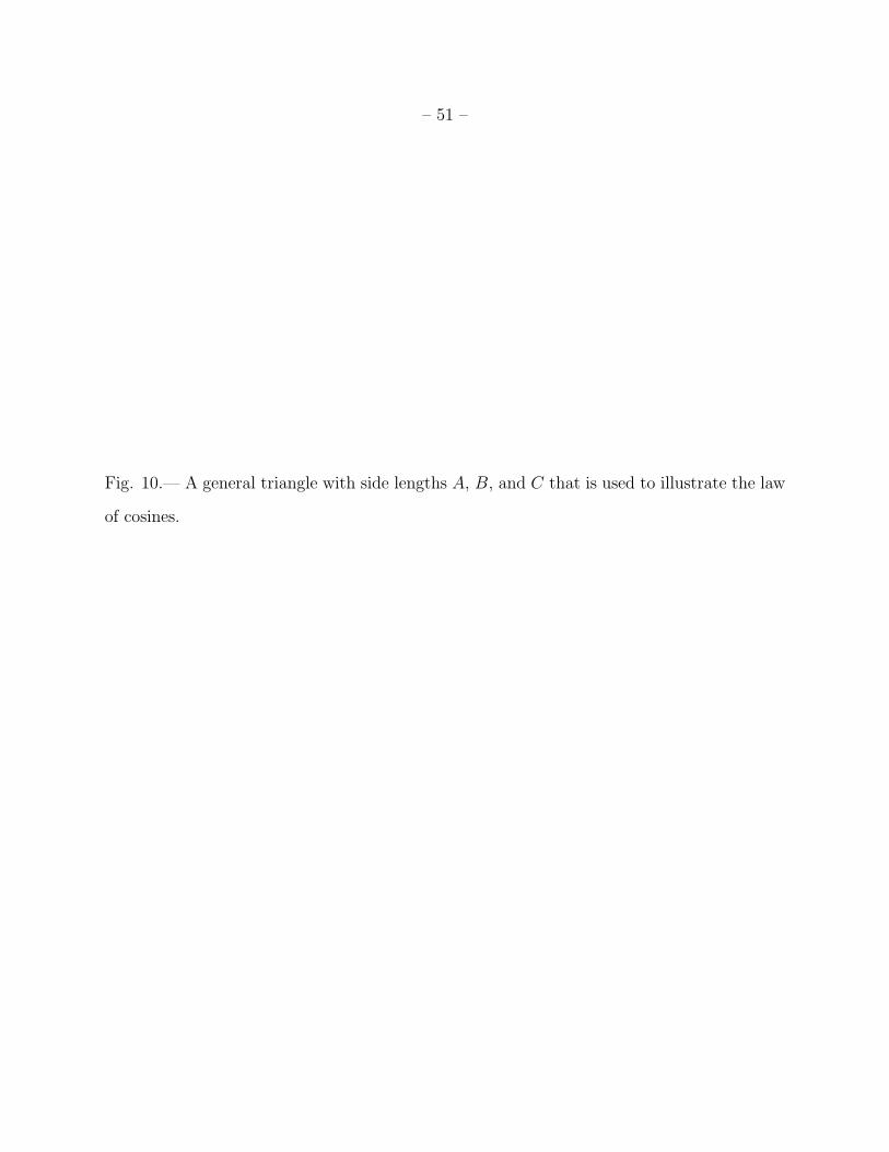
Fig. 10.— A general triangle with side lengths A, B, and C that is used to illustrate the law
of cosines.

– 52 –
What is θ. Well from Figure 10, it clear that θ is the angle between ~B’s tail is put at
the head of ~A. In other words, it’s the angle subtended by side C of the triangle formed by
the side lengths A, B, and C.
Since A and B are general lengths, we have generally for a triangle of side lengths A,
B, and C that
C2 = A2 + B2 − 2AB cos θ , (114)
where θ is angle subtended by side C.
This last formula is the law of cosines.
8.6. Triangle Inequality
Consider the law of cosines for a general triangle with side lengths A, B, and C:
C2 = A2 + B2 − 2AB cos θ , (115)
where θ is angle subtended by side C.
Fig. 11.— The triangle inequality illustrated.

– 53 –
Now
C2 = A2 + B2 − 2AB cos θ
≤ A2 + B2 + |2AB cos θ|
= A2 + B2 + 2AB| cos θ|
≤ A2 + B2 + 2AB = (A + B)2 , (116)
where we’ve used that fact that A and B are greater than zero and | cos θ ≤ 1 always.
Thus, we find that
C ≤ A + B (117)
which is the triangle inequality.
In words, the triangle inequality is that the sum of two side lengths of a triangle is
always less than or equal to the third side length.
We illustrate the triangle inequality in Figure 11.
The equality only holds when | cos θ| = 1 which means that the triangle has collapsed
to a line. Now | cos θ| = 1 means that or θ = 0◦ or θ = 180◦. If θ = 0◦, then one of A and B
is zero and the other of A and B equals C and is collinear with C. If θ = 180◦, then sides
A and B are collinear and collinear with side C.
8.7. The Law of Sines
To prove the law of sines consider a general triangle with side lengths A, B, and C.
Let side C be the base.
Say side C is collinear with a base line.
Let y be the length of a perpendicular from the vertex opposite side C to the base line.

– 54 –
Let side B be to the right than side A.
Now both sides A and B are hypotenuses of right triangles formed by themselves, the
perpendicular, and segments along the base line.
We illustrate the situation in Figure 12.
Fig. 12.— Illustration of the triangle used to prove the law of sines.
– 55 –
Now
y = A sin θB and y = B sin θA,sup , (118)
where θB is the angle of the general triangle opposite side B and θA,sup is the supplementary
angle to θA which is the angle of the general triangle opposite side A.
Note θA,sup = 180◦ − θA and sin(180◦ − θA) = sin θA by a trig identity from Table 1.
Since y is equal to y, we obtain
A sin θB = B sin θA andsin θA
A=
sin θB
B. (119)
The last result does not depend on side B being to the right of side A. If we flipped
triangle laterally, side A would have been to the right of side B. Following the same steps,
we would have gotten the same result.
So the result holds no matter which of side A and B is to the right of the other.
Also not if we had chosen A to be the base by the same steps we would have found
sin θB
B=
sin θC
C(120)
no matter which of side B and C is to the left of the other.
So we conclude for a general triangle that
sin θA
A=
sin θB
B=
sin θC
C. (121)
It doesn’t matter which side you label A, B, or C since the sides were chosen arbitrarily
in the proof.
The result equation (121) is the law of sines.
The reciprocal result is also called the law of sinces: i.e.,
A
sin θA
=B
sin θB
=C
sin θC
. (122)

– 56 –
ACKNOWLEDGMENTS
Support for this work has been provided by the Department of Physics of the University
of Idaho and the Department of Physics of the University of Oklahoma.
A. MORE TRIGONOMETRIC IDENTITIES
We can prove a few more trig identities appearing Table 1. The proofs are simple given
the trig identities proven in §§ 2 and 8.
We won’t tediously describe what identities we use in the proofs. They are self-identified.
A.1. Identities for Argument θ ± 180◦
Behold:
sin(θ ± 180◦) = sin(θ) cos(±180◦) + cos(θ) sin(±180◦) = − sin(θ) , (A1)
cos(θ ± 180◦) = cos(θ) cos(±180◦) − sin(θ) sin(±180◦) = − cos(θ) , (A2)
tan(θ ± 180◦) =sin(θ ± 180◦)
cos(θ ± 180◦)= tan(θ) , (A3)
whence
sin(θ ± 180◦) = − sin(θ) , (A4)
cos(θ ± 180◦) = − cos(θ) , (A5)
tan(θ ± 180◦) = tan(θ) . (A6)
We not that the tangent function is period over 180◦ as well as over 360◦.
– 57 –
A.2. Identities for Argument 180◦ − θ
Behold:
sin(180◦ − θ) = − sin(θ − 180◦) = sin(θ) , (A7)
cos(180◦ − θ) = cos(θ − 180◦) = − cos(θ) , (A8)
tan(180◦ − θ) = − tan(θ − 180◦) = − tan(θ) , (A9)
whence
sin(180◦ − θ) = sin(θ) , (A10)
cos(180◦ − θ) = − cos(θ) , (A11)
tan(180◦ − θ) = − tan(θ) . (A12)
A.3. Identities for Argument θ ± 90◦
Behold:
sin(θ ± 90◦) = sin(θ) cos(±90◦) + cos(θ) sin(±90◦) = ± cos(θ) , (A13)
cos(θ ± 90◦) = cos(θ) cos(±90◦) − sin(θ) sin(±90◦) = ∓ sin(θ) , (A14)
tan(θ ± 90◦) =sin(θ ± 90◦)
cos(θ ± 90◦)=
± cos(θ)
∓ sin(θ)= − 1
tan(θ)= − cot(θ) , (A15)
whence
sin(θ ± 90◦) = ± cos(θ) , (A16)
cos(θ ± 90◦) = ∓ sin(θ) , (A17)
tan(θ ± 90◦) = − 1
tan(θ)= − cot(θ) , (A18)

– 58 –
A.4. Identities for Argument 90◦ − θ
Behold:
sin(90◦ − θ) = − sin(θ − 90◦) = cos(θ) , (A19)
cos(90◦ − θ) = cos(θ − 90◦) = sin(θ) , (A20)
tan(90◦ − θ) = − tan(θ − 90◦) =1
tan(θ)= cot(θ) , (A21)
whence
sin(90◦ − θ) = cos(θ) , (A22)
cos(90◦ − θ) = sin(θ) , (A23)
tan(90◦ − θ) =1
tan(θ)= cot(θ) . (A24)
A.5. Identity cos(a) cos(b) =1
2[cos(a − b) + cos(a + b)]
Add the expansions for cos(a − b) and cos(a + b) to get
cos(a − b) + cos(a + b) = 2 cos(a) cos(b) (A25)
which yields immediately
cos(a) cos(b) =1
2[cos(a − b) + cos(a + b)] . (A26)
If a = b, we get
cos2(a) =1
2[1 + cos(2a)] . (A27)
A.6. Identity sin(a) sin(b) =1
2[cos(a − b) − cos(a + b)]
Subtract form the expansions for cos(a − b) the expansion from cos(a + b) to get
cos(a − b) − cos(a + b) = 2 sin(a) sin(b) (A28)

– 59 –
which yields immediately
sin(a) sin(b) =1
2[cos(a − b) − cos(a + b)] . (A29)
If a = b, we get
sin2(a) =1
2[1 − cos(2a)] . (A30)
A.7. Identity sin(a) cos(b) =1
2[sin(a − b) + sin(a + b)]
Add the expansions for sin(a + b) and sin(a − b) to get
sin(a + b) + sin(a − b) = 2 sin(a) cos(b) (A31)
which yields immediately
sin(a) cos(b) =1
2[sin(a − b) + sin(a + b)] . (A32)
If a = b, we get
sin(a) cos(a) =1
2sin(2a)] . (A33)
REFERENCES
Arfken, G. 1970, Mathematical Methods for Physicists (New York: Academic Press)
Barger, V. D., & Olson, M. G. 1987, Classical Electricity and Magnetism (Boston: Allyn
and Bacon, Inc.)
Enge, H. A. 1966, Introduction to Nuclear Physics (Reading, Massachusetts: Addison-Wesley
Publishing Company)

– 60 –
Griffiths, D. J. 1999, Introduction to Electrodynamics (Upper Saddle River, New Jersey:
Prentice Hall)
Ohanian, H. C. 1988, Classical Electrodynamics (Boston: Allyn and Bacon, Inc.)
Serway, R. A. & Jewett, J. W., Jr. 2008, Physics for Scientists and Engineers, 7th Edition
(Belmont, California: Thomson)
Tipler, P. A., & Mosca, G. 2008, Physics for Scientists and Engineers, 6th Edition (New
York: W.H. Freeman and Company)
Weber, H. J., & Arfken, G. B. 2004, Essential Mathematical Methods for Physicists (Ams-
terdam: Elsevier Academic Press)
Wolfson, R. & Pasachoff, J. M. 1990, Physics: Extended with Modern Physics (London:
Scott, Foresman/Little, Brown Higher Education)
This preprint was prepared with the AAS LATEX macros v5.2.