Vector Generalized Additive Modelsand applications to extreme value

analysis

Olivier Mestre (1,2)

(1) Météo-France, Ecole Nationale de la Météorologie, Toulouse, France(2) Université Paul Sabatier, LSP, Toulouse, France

Based on previous studies realized in collaboration with :Stéphane Hallegatte (CIRED, Météo-France)Sébastien Denvil (LMD)

SMOOTHER

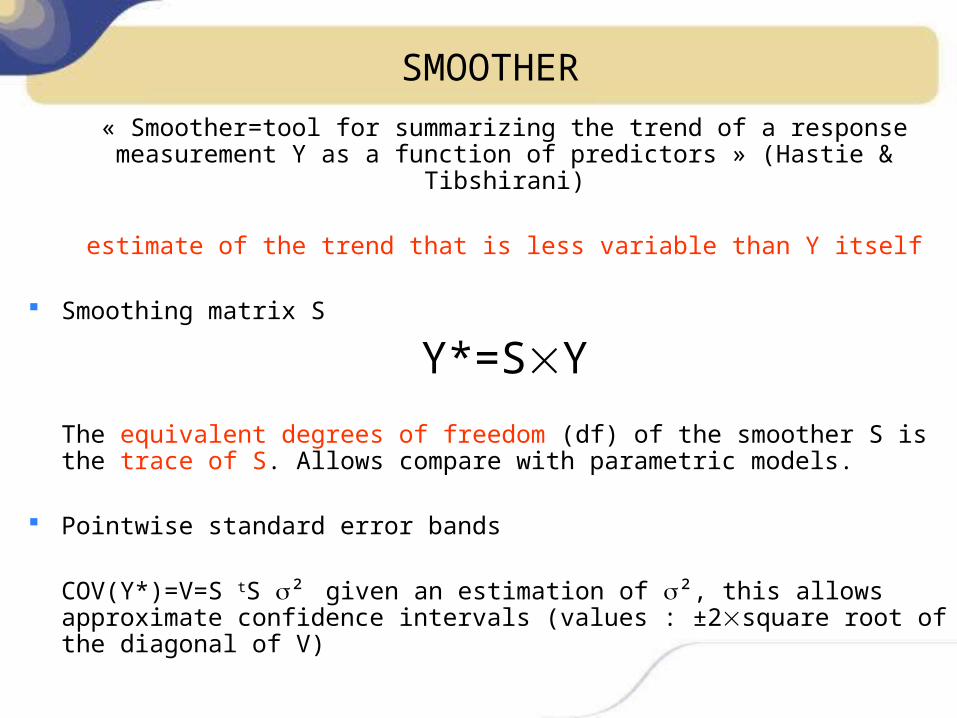
« Smoother=tool for summarizing the trend of a response measurement Y as a function of predictors » (Hastie & Tibshirani)

estimate of the trend that is less variable than Y itself

Smoothing matrix S

Y*=SY

The equivalent degrees of freedom (df) of the smoother S is the trace of S. Allows compare with parametric models.

Pointwise standard error bands

COV(Y*)=V=S tS ² given an estimation of ², this allows approximate confidence intervals (values : ±2square root of the diagonal of V)

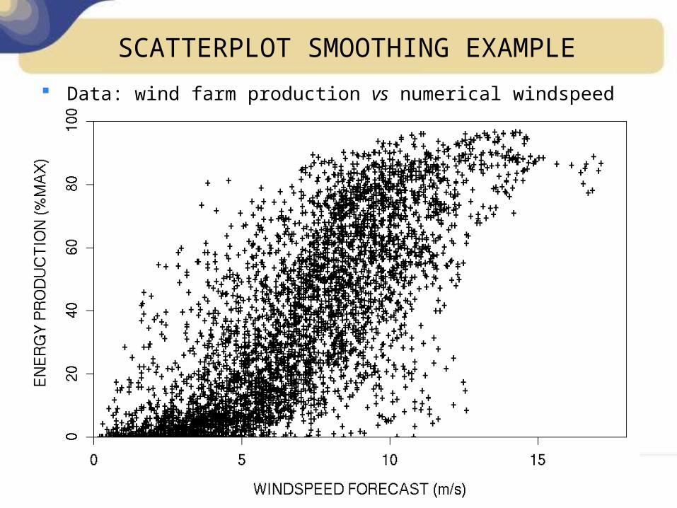
SCATTERPLOT SMOOTHING EXAMPLE

Data: wind farm production vs numerical windspeed forecasts

SMOOTHING

Problems raised by smoothers

How to average the response values in each neighborhood?

How large to take the neighborhoods?

Tradeoff between bias and variance of Y*

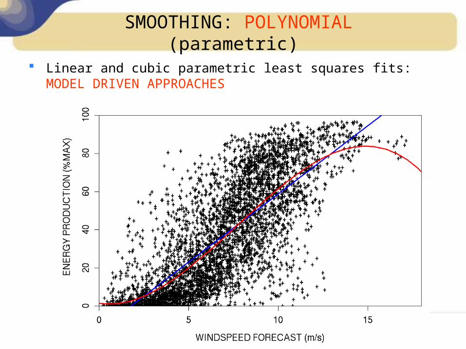
SMOOTHING: POLYNOMIAL (parametric)

Linear and cubic parametric least squares fits: MODEL DRIVEN APPROACHES

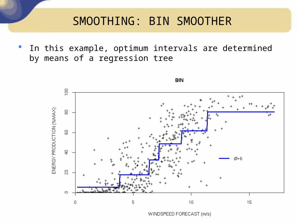
SMOOTHING: BIN SMOOTHER

In this example, optimum intervals are determined by means of a regression tree

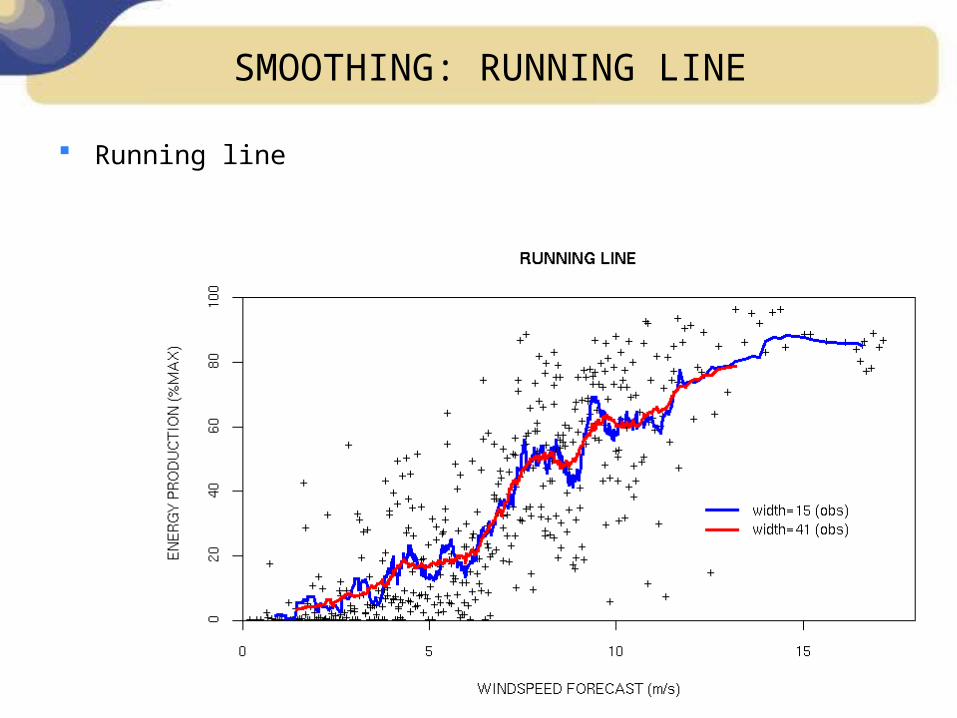
SMOOTHING: RUNNING LINE

Running line

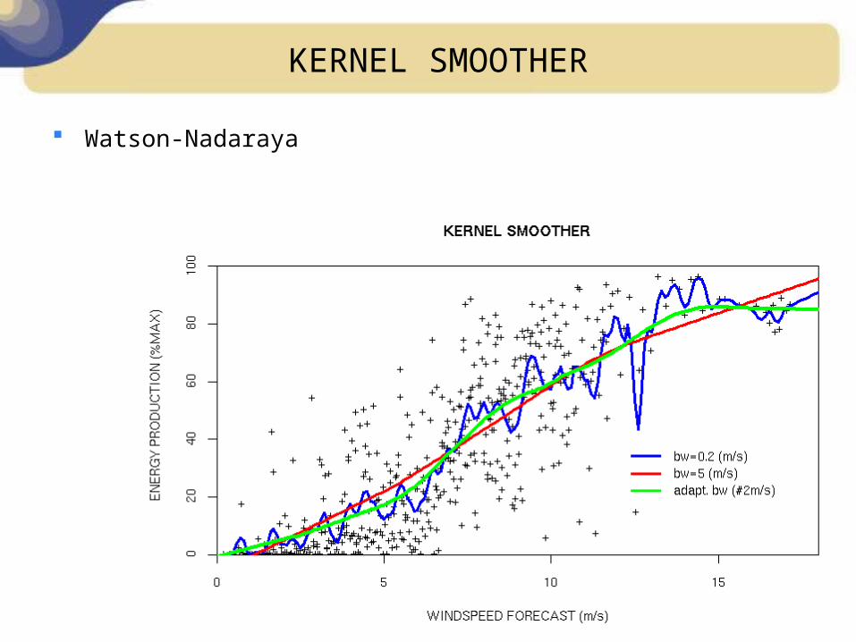
KERNEL SMOOTHER

Watson-Nadaraya

SMOOTHING: LOESS

The smooth at the target point is the fit of a locally-weighted linear fit (tricube weight)

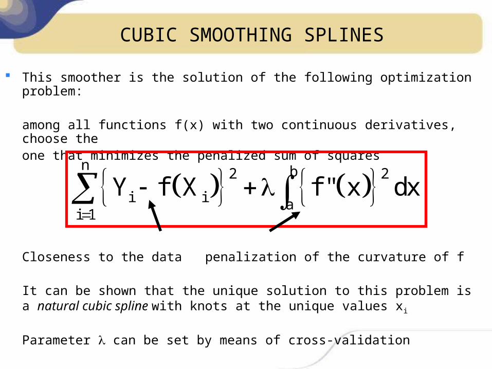
CUBIC SMOOTHING SPLINES

This smoother is the solution of the following optimization problem:

among all functions f(x) with two continuous derivatives, choose theone that minimizes the penalized sum of squares

Closeness to the data penalization of the curvature of f

It can be shown that the unique solution to this problem is a natural cubic spline with knots at the unique values xi

Parameter can be set by means of cross-validation

n b2 2

i i ai 1

Y f X f " x dx

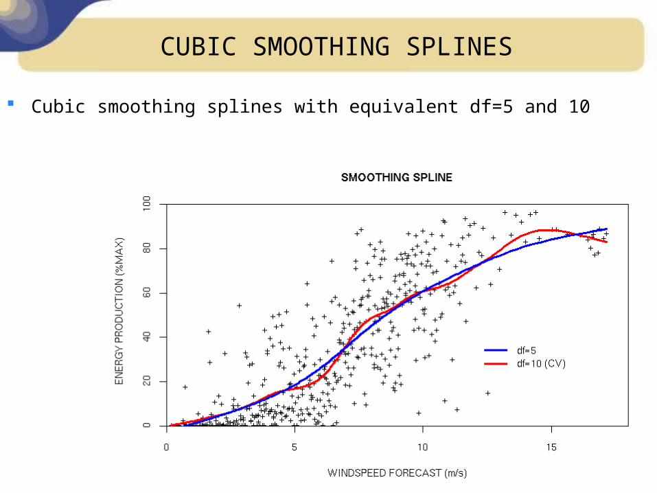
CUBIC SMOOTHING SPLINES

Cubic smoothing splines with equivalent df=5 and 10

Additive models

Gaussian Linear Model : IE[Y]=o+1X1+2X2

Gaussian Additive model : IE[Y]=S1(X1)+S2(X2)

S1, S2 smooth functions of predictors X1, X2, usually LOESS, SPLINE

Estimation of S1, S2 : « Backfitting Algorithm »

PRINCIPLE OF THE BACKFITTING ALGORITHM

Y=S1(X1)+e estimation S1*

Y-S1*(X1)=S2(X2)+e estimation S2*

Y-S2*(X2)=S1(X1)+e estimation S1**

Y-S1**(X1)=S2(X2)+e estimation S2**

Y-S2**(X2)=S1(X1)+e estimation S1***

Etc… until convergence

Additive models

Additive models

One efficient way to perform non-linear regression, but…

Crucial point

ADAPTED WHEN ONLY FEW PREDICTORS

2, 3 predictors at most

Additive models

Philosophy

DATA DRIVEN APPROACHES RATHER THAN MODEL DRIVEN APPROACH

USEFUL AS EXPLORATORY TOOLS

Approximate inference tests are possible, but full inferences are better assessed by means of parametric models

Generalized Additive models (GAM)

Extension to non-normal dependant variables

Generalized additive models : additive modelling of the natural

parameter of exponential family laws (Poisson, Binomial, Gamma, Gauss…).

g[µ]==S1(X1)+S2(X2)

Vector Generalized Additive Models (VGAM): one step beyond…

Example 1

Annual umber and maximum integrated intensity (PDI) of hurricane tracks

over the North Atlantic

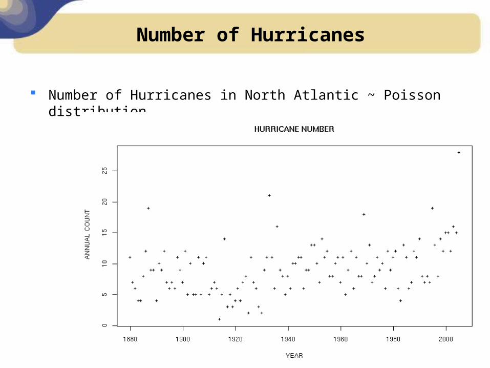
Number of Hurricanes

Number of Hurricanes in North Atlantic ~ Poisson distribution

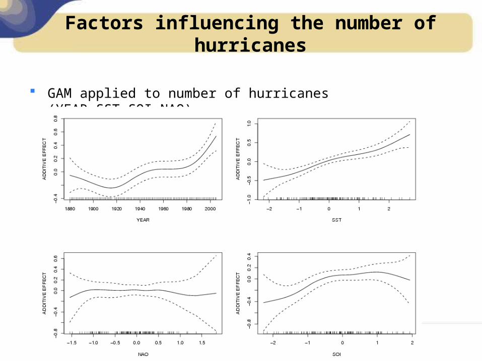
Factors influencing the number of hurricanes

GAM applied to number of hurricanes (YEAR,SST,SOI,NAO)

GAM model

Log()= o+S1(SST)+S2(SOI)

PARAMETRIC model

“broken stick model” (with continuity constraint) in SOI, revealed by GAM analysis

log() = o+SOI(1)SOI+SSTSST SOI<K

= o+SOI(1)SOI+SOI

(2)(SOI-K)+SSTSST SOIK

The best fit obtained for SOI value K=1

log-likelihood=-316.16, to be compared with -318.71 (linearity)

standard deviance test allows reject linearity (p value=0.02)

Expectation of the hurricane number is then straightforwardly computed as a function of SOI and SST

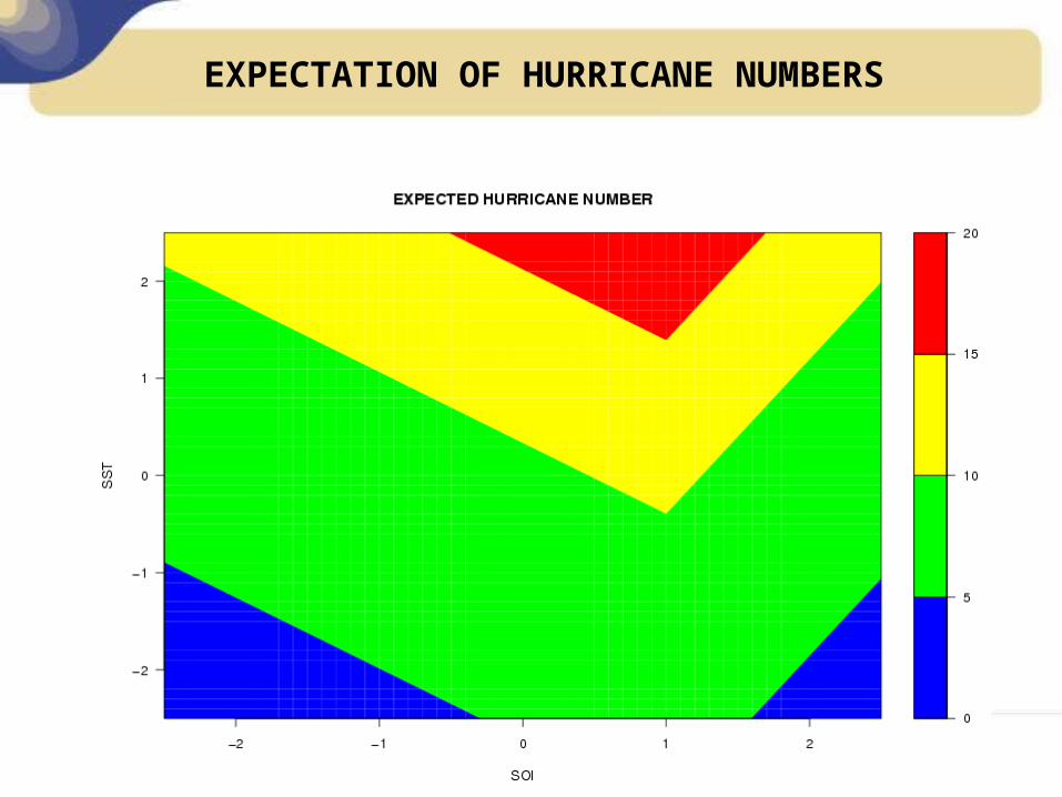
EXPECTATION OF HURRICANE NUMBERS

OBSERVED vs EXPECTED: r=0.6