Vector Chiral Phases in FrustratedSystems

Inaugural-Dissertationzur

Erlangung des Doktorgradesder Mathematisch-Naturwissenschaftlichen Fakultät

der Universität zu Kölnvorgelegt von

Hannes Schenckaus Berlin-Wilmersdorf

Universität zu Köln2015

Berichterstatter: Prof. Dr. Thomas NattermannProf. Dr. Joachim Krug

Tag der letzten mündlichen Prüfung: 23.06.2015

Diese Arbeit ist meinen Eltern Ingolf & Annette gewidmet

Zusammenfassung

Die vorliegende Dissertation setzt sich aus zwei verschiedenen Teilen zusammen. Der erste Teilder Arbeit befasst sich mit der Untersuchung von chiraler Ordnung und ihrem Ursprung infrustrierten Wechselwirkungen. Zunächst wird das Konzept von Phasenübergängen und derenRelation zu der dem System zugrunde liegenden Symmetrie beschrieben. Hier wird diskutiertwie die diskrete Z2-Symmetrie der Ising-Spins und die kontinuierliche SO(2)-Symmetrie der XY-Spins in zwei Dimensionen zu fundamental verschiedenen Phasenübergängen führen. Als nächsteswerden verschiedene Formen von chiraler Ordnung diskutiert, sowie deren experimentelle Rea-lisierung. Chirale Ordnung bricht die diskrete Inversions-Symmetrie (Z2), die simultan mit derSO(2)-Symmetrie der XY-Spins auftreten kann. Eine zentrale Fragestellung der Arbeit ist, zuklären, wie die Phasenübergänge sich durch das Auftreten der zusätzlichen Symmetrien verän-dern. Als archetypisches Modell für das gleichzeitige Auftreten von diskreter und kontinuierlicherSymmetrie wird das sogenannte helikale XY-Modell untersucht. Das Modell selbst wird als Er-weiterung des klassischen XY-Modells eingeführt und ausführlich diskutiert. Es wird beschrieben,wie durch die Einführung einer frustrierten Wechselwirkung das System einen chiralen Grund-zustand ausbilden kann und welche verschiedenen Ansätze es gibt, die simultanen Symmetrienzu untersuchen. Zusätzlich wird eine mesoskopische Version des Modells abgeleitet.

Zunächst wird der Phasenübergang der chiralen Ordnung diskutiert. Hier wird mittels des Va-riationsprinzips die kritische Temperatur für den Übergang gefunden sowie die Abhängigkeit derTemperatur vom Spiral-Winkel θ der Grundzustandsspirale. Anschließend wird der Effekt vonchiraler Ordnung auf den Berezinskii-Kosterlitz-Thouless (BKT) Übergang der SO(2)-Symmetriein dem Modell untersucht. Die für den BKT-Übergang verantwortlichen Vortizes werden auf klei-nen und großen Skalen diskutiert und die Energiekosten des Vortex-Kerns abgeschätzt. MittelsRenormierungsgruppen-Rechnung werden die Effekte der Vortizes auf den Phasenübergang un-tersucht und deren kritische Exponenten bestimmt. Anschließend wird die anomale Skalierungs-dimension des chiralen Übergangs bestimmt. Die Daten der numerischen Simulationen von Soro-kin et al. werden verwendet, um die kritischen Exponenten zu bestimmen und mit den errechne-ten Werten zu vergleichen. Das entstehende Phasendiagramm wird beschrieben sowie möglicheexperimentelle Systeme und die Relation zu anderen theoretischen Arbeiten werden diskutiert.

Weiterführend wird näher auf den Zusammenhang zwischen chiraler Ordnung und Polari-sation in multiferroischen Systemen eingegangen. Verschiedene Mechanismen für die Kopplungvon magnetischer und elektrischer Ordnung werden diskutiert und ausgehend von Symmetrie-Überlegungen wird das HXY-Modell um eine Wechselwirkung mit einem elektrischen Feld er-weitert. Diskutiert werden die Effekte der Polarisation auf die Domänenwände im System. Dieresultierenden Sattelpunktsgleichungen werden näherungsweise gelöst und mit numerischen Re-sultaten verglichen. Des Weiteren wird die effektive Wechselwirkung zwischen den chiralen Domä-nenwände und den Domänenwänden in der Polarisation ermittelt und als gegenseitige Anziehungidentifiziert.

Als konkretes Beispiel eines multiferroischen Materials wird das Material MnWO4 näher dis-kutiert. Hier koppelt chirale Ordnung an Polarisation gekennzeichnet durch einen magnetischenPhasenübergang, der mit dem Auftreten einer messbaren Polarisation einhergeht. Hier wurde inZusammenarbeit mit der Arbeitsgruppe von Prof. J. Hemberger das kritische Verhalten an demPhasenübergang untersucht. Zunächst werden die beobachteten Phasenübergänge in MnWO4

iii

beschrieben und näher auf die Kristallsymmetrie eingegangen. Ausgehend von der von Tolédanobestimmten Ginzburg-Landau Freien Energie des Systems wird der Phasenübergang klassifiziertund das kritische dynamische Verhalten bestimmt. Die resultierenden Exponenten werden mitder experimentellen Arbeit der Arbeitsgruppe von Prof. J. Hemberger verglichen.

Im zweiten Teil der Arbeit wird das dynamische Verhalten von Vortizes in dünnen supra-leitenden Filmen untersucht. Zunächst wird ein historischer Überblick über die Entdeckung derSupraleitung gegeben und anschließend auf deren phänomenologische Beschreibung eingegangen.Danach wird das Phänomen von supraleitenden Vortizes diskutiert und auf die Besonderheitenvon Vortizes in dünnen Filmen eingegangen sowie deren Wechselwirkung mit einem extern an-gelegten Strom.

Zu Beginn wird der experimentelle Aufbau, der von der Arbeitsgruppe um Prof. E. Zeldovverwendet wird, beschrieben. Studiert werden hier Vortizes in dünnen supraleitenden Blei Filmenmittels SQUID-on-tip Raster-Mikroskopie. Bei angelegtem Strom können Vortizes in den Filmeintreten indem sie eine Eintrittsbarriere überwinden. Diese Barrieren werden diskutiert und derEffekt auf die messbaren Strom-Spannungskurven wird bestimmt. Die Resultate werden mit denzur Verfügung stehenden experimentellen Werten verglichen.

Abschließend wird die Dynamik der Vortizes in den Filmen untersucht. Hier liegt das Augen-merk vor allem auf dem Effekt einer inhomogenen Stromdichte resultierend aus der experimentellangebrachten Verengung der dünnen Bleistreifen. Erklärt werden soll die Linienbildung der sichbewegenden Vortices, sowie das Entstehen von Verzweigungspunkten in diesen Linien. Es wer-den verschiedene Ansätze und effektive Modelle für die wechselwirkenden Vortizes diskutiert undderen Schwachstellen dargestellt.

iv

Abstract

The present dissertation consists of two parts. The first part of this work deals with the study ofchiral order that has its origin in frustrated interactions. First of all, the basic concept of phasetransitions and their relation to the underlying symmetry will be described. Here we will discusshow the discrete Z2 symmetry of the Ising spins and the continuous SO(2) symmetry of the XYspins leads to fundamentally different phase transitions. Next, different forms of chiral orderwill be discussed, as well as their experimental realizations. Chiral order breaks the discreteinversion symmetry (Z2), which can appear simultaneously with the SO(2) symmetry of the XYspins. One of the central questions of this work is how the phase transitions are influenced bythe additional symmetries. As an archetypical model for the simultaneous existence of both adiscrete and continuous symmetry, the so-called helical XY model will be studied. The modelitself will be introduced as an extension to the classical XY model and will be discussed in detail.It will be described how the addition of a frustrated interaction leads to a chiral ground state anddifferent approaches to dealing with these simultaneous symmetries are mentioned. Additionally,the mesoscopic version of the model will be derived.

We will start with the discussion of the chiral order phase transition. Using a variationalmethod, the critical temperature of the transition and its dependance on the chiral pitch angleθ will be found. Afterwards, the effect of the chiral order on the Berezinskii–Kosterlitz–Thouless(BKT) transition of the SO(2) symmetry will be studied. The vortices responsible for the BKTtransition will be discussed on short and large length scales and the energy cost of the vortexcores is estimated. Using the renormalization group technique, the effects of the vortices on thephase transition is studied and their critical exponents are estimated. Afterwards, the anomalousscaling dimension of the chiral transition is calculated. The data of the numerical simulationsdone by Sorokin et al. are used to determine the critical exponents and compare them to theanalytic calculations. The resulting phase diagram for the HXY model is calculated and itsrelation to possible experimental systems and other theoretical works is discussed.

We will continue with a closer look at the relation between chiral order and polarizationin multiferroic systems. Different mechanisms for the coupling of magnetic and electric orderare discussed and, starting from a symmetry argument, the HXY model will extended by aninteraction with the electric field. The effect of the polarization on the domain walls of thesystem will be studied. The resulting saddle-point equations will be solved perturbatively and arecompared to numerical results. Additionally, an effective interaction between the chiral domainwalls and the polarization walls will be derived and identified as an attractive interaction.

As a concrete example of a multiferroic material, the material MnWO4 will be studied. Herethe chiral order couples to the polarization, as indicated by a magnetic phase transition withan accompanied onset of polarization. In collaboration with D. Niermann and the group ofProf. J. Hemberger, the critical behavior of the phase transition was studied. First the differentphase transitions in MnWO4 will be described and the crystal symmetry will be discussed. Start-ing from the Ginzburg–Landau free energy expansion done by Tolédano, the phase transitionswill be classified and the critical dynamical behavior described. The resulting critical exponentsare compared to the experimental work of the group of Prof. J. Hemberger.

In the second part of this work, the dynamical behavior of vortices in thin superconductingfilms is studied. First, a historical overview of the discovery of superconductivity is given,

v

followed by a discussion of it phenomenological description. Afterwards, the phenomenon ofsuperconducting vortices is discussed and the special features of vortices in thin films and theirinteraction with an applied current are presented.

We start with a description of the experimental setup used in the group of Prof. E. Zeldov.They study vortices in thin superconducting lead films with the SQUID-on-tip raster microscopy.In the presence of an applied current, vortices can enter the thin strips by overcoming an entrybarrier. These barriers are discussed and their effect on the measurable current–voltage curvesis calculated. The results are compared to the available numerical data.

Finally, we study the dynamics of the vortices in thin films. The focus is on the effect ofinhomogeneous current densities, a result from experimentally imposed constrictions in the thinfilms themselves. The task is to explain the formation of lines in the moving vortices and theexistence of bifurcation points in said lines. Several approaches and effective models are used tostudy the interacting vortices, the results and shortcomings are discussed.

vi

Contents

Contents vii

I Vector-Chirality and Spin-Liquid in Frustrated Systems 1

1 Introduction 31.1 Magnetic systems . . . . . . . . . . . . . . . . . . . . . . . . . . . . . . . . . . . . 41.2 Discrete and continuous symmetry in ferromagnets . . . . . . . . . . . . . . . . . 61.3 Vector and scalar chiral order parameters . . . . . . . . . . . . . . . . . . . . . . 91.4 Physical realizations and experimental systems . . . . . . . . . . . . . . . . . . . 111.5 Outline . . . . . . . . . . . . . . . . . . . . . . . . . . . . . . . . . . . . . . . . . 13

2 The Model 152.1 The classical model . . . . . . . . . . . . . . . . . . . . . . . . . . . . . . . . . . . 152.2 Quantum chain . . . . . . . . . . . . . . . . . . . . . . . . . . . . . . . . . . . . . 202.3 Landau–Ginzburg–Wilson Hamiltonian . . . . . . . . . . . . . . . . . . . . . . . . 22

3 Chiral Transition 273.1 The variational approach . . . . . . . . . . . . . . . . . . . . . . . . . . . . . . . 273.2 The solutions . . . . . . . . . . . . . . . . . . . . . . . . . . . . . . . . . . . . . . 313.3 Discussion . . . . . . . . . . . . . . . . . . . . . . . . . . . . . . . . . . . . . . . . 33

4 Renormalization Group 354.1 Vortices . . . . . . . . . . . . . . . . . . . . . . . . . . . . . . . . . . . . . . . . . 354.2 Long–range interaction in Ising order parameter model . . . . . . . . . . . . . . . 364.3 RG - small scales . . . . . . . . . . . . . . . . . . . . . . . . . . . . . . . . . . . . 374.4 RG - large scales . . . . . . . . . . . . . . . . . . . . . . . . . . . . . . . . . . . . 384.5 Anomalous dimension of chiral transition . . . . . . . . . . . . . . . . . . . . . . 424.6 Comparison to numerics . . . . . . . . . . . . . . . . . . . . . . . . . . . . . . . . 444.7 Phase diagram . . . . . . . . . . . . . . . . . . . . . . . . . . . . . . . . . . . . . 454.8 Discussion . . . . . . . . . . . . . . . . . . . . . . . . . . . . . . . . . . . . . . . . 48

5 Multiferroics 535.1 Connection between chiral order and polarization . . . . . . . . . . . . . . . . . . 545.2 One–dimensional domain wall . . . . . . . . . . . . . . . . . . . . . . . . . . . . . 565.3 Two–dimensional domain wall . . . . . . . . . . . . . . . . . . . . . . . . . . . . . 655.4 Domain wall in “four-state” model . . . . . . . . . . . . . . . . . . . . . . . . . . 67

6 MnWO4 716.1 Material properties and observed phase transitions . . . . . . . . . . . . . . . . . 716.2 Group theory construction of Ginzburg–Landau free energy . . . . . . . . . . . . 716.3 Classification of phase transitions and critical dynamics . . . . . . . . . . . . . . 746.4 Dynamical exponent at AF3 → AF2 . . . . . . . . . . . . . . . . . . . . . . . . 76

vii

Contents Contents

6.5 Discussion . . . . . . . . . . . . . . . . . . . . . . . . . . . . . . . . . . . . . . . . 79

II Vortices in Supraconducting Thin Films 81

7 Introduction 83

8 Experimental Data 858.1 Experimental setup . . . . . . . . . . . . . . . . . . . . . . . . . . . . . . . . . . . 858.2 Current–Voltage curves . . . . . . . . . . . . . . . . . . . . . . . . . . . . . . . . 888.3 Vortex dynamics . . . . . . . . . . . . . . . . . . . . . . . . . . . . . . . . . . . . 89

9 Superconductivity 919.1 Vortices . . . . . . . . . . . . . . . . . . . . . . . . . . . . . . . . . . . . . . . . . 939.2 Vortex interaction . . . . . . . . . . . . . . . . . . . . . . . . . . . . . . . . . . . 95

10 Current–Voltage Curves 9710.1 Bardeen–Stephen flow . . . . . . . . . . . . . . . . . . . . . . . . . . . . . . . . . 9910.2 Surface barrier . . . . . . . . . . . . . . . . . . . . . . . . . . . . . . . . . . . . . 10110.3 Discussion . . . . . . . . . . . . . . . . . . . . . . . . . . . . . . . . . . . . . . . . 106

11 Vortex Dynamics 10711.1 The Corbino disk setup . . . . . . . . . . . . . . . . . . . . . . . . . . . . . . . . 10711.2 The current distribution in the Corbino disk . . . . . . . . . . . . . . . . . . . . . 10911.3 Non–local theory . . . . . . . . . . . . . . . . . . . . . . . . . . . . . . . . . . . . 11011.4 Simple model for current–vortex interaction . . . . . . . . . . . . . . . . . . . . . 11411.5 Vortex–Current interaction - thin strip . . . . . . . . . . . . . . . . . . . . . . . . 11711.6 Vortex–Current interaction - Corbino disk . . . . . . . . . . . . . . . . . . . . . . 12011.7 Discussion . . . . . . . . . . . . . . . . . . . . . . . . . . . . . . . . . . . . . . . . 123

IIIAppendix 125

A Appendix: Model 127A.1 XY quantum chain . . . . . . . . . . . . . . . . . . . . . . . . . . . . . . . . . . . 127A.2 Kolezhuk mapping . . . . . . . . . . . . . . . . . . . . . . . . . . . . . . . . . . . 129

B Appendix: Renormalization Group 131B.1 Vortex core energy integral . . . . . . . . . . . . . . . . . . . . . . . . . . . . . . 131B.2 Fourier transform in x-direction . . . . . . . . . . . . . . . . . . . . . . . . . . . . 132B.3 Calculating the constant pre-factor f(0) . . . . . . . . . . . . . . . . . . . . . . . 133B.4 Calculating the f(z →∞) limit . . . . . . . . . . . . . . . . . . . . . . . . . . . . 135B.5 Solving the full Fourier transform . . . . . . . . . . . . . . . . . . . . . . . . . . . 135B.6 Solving f(z) via ODE . . . . . . . . . . . . . . . . . . . . . . . . . . . . . . . . . 136B.7 Numerical calculation of the constant cx . . . . . . . . . . . . . . . . . . . . . . . 137B.8 Numerical data from Sorokin et al. . . . . . . . . . . . . . . . . . . . . . . . . . . 138

C Appendix: Multiferroics 141C.1 Integral Approximation . . . . . . . . . . . . . . . . . . . . . . . . . . . . . . . . 141C.2 Python code for numerics . . . . . . . . . . . . . . . . . . . . . . . . . . . . . . . 142

viii

D Appendix: MnWO4 147D.1 Different forms of order parameters . . . . . . . . . . . . . . . . . . . . . . . . . . 147D.2 Transition at TN : temperature fluctuations in S1 . . . . . . . . . . . . . . . . . . 148D.3 Transition at T2: Frozen S1 order parameter . . . . . . . . . . . . . . . . . . . . . 150

E Appendix: Experiment 153E.1 Material properties of lead . . . . . . . . . . . . . . . . . . . . . . . . . . . . . . . 153

F Appendix: Vortex Dynamics 155F.1 Detailed overview of current distribution . . . . . . . . . . . . . . . . . . . . . . . 155F.2 Derivation of main equations . . . . . . . . . . . . . . . . . . . . . . . . . . . . . 159F.3 Limiting cases and solutions to integral equations . . . . . . . . . . . . . . . . . . 162F.4 Numerical approach . . . . . . . . . . . . . . . . . . . . . . . . . . . . . . . . . . 165

Bibliography 171

ix

Part I

Vector-Chirality and Spin-Liquid inFrustrated Systems

1. Introduction

A material can be classified by its macroscopic properties such as density, volume, magnetization,resistivity and many more. In some cases, the macroscopic state can be changed by continuouslyvarying an external parameter, such as the temperature, the applied magnetic field or the pres-sure. The system will undergo an abrupt change in one or more of its physical properties at acertain point in the parameter space of the external fields.

There are many examples of phase transitions in nature. To give a little idea of their diversity,we want to name just a few. The most commonly known example is the melting of a solid, as canbe seen in water when melting an ice cube. Here the system changes from a ridged solid to a fluid.Another example is the ferromagnet to paramagnet transition in magnetic materials such as iron(Fe). Here, the magnetization vanishes at the Curie temperature when heating up the material.There are also structural phase transitions. In the material bariumtitanat (BaTiO3), varying thetemperature results in a change of the crystal structure, [1]. This is is accompanied by a resultingelectric dipole moment in each crystal cell and a global electric polarization. Another famousexample are superconductors like lead (Pb). Here, the system switches from a finite resistanceto superconductivity after the system is cooled below a critical temperature. A more detailedlist and other examples can be found in standard literature such as [1, 2].

Essentially there are two ways in which a system can change from one phase to another. In thefirst case, the phases on either side of the transition line also coexist exactly at the transition,[3]. The phases still carry their distinct microscopical properties and are still distinguishablefrom each other despite the system being at phase transition. Away from the transition, thesystem will be in a unique phase that is continuously connected to the coexistence phase at thetransition. One example for this type of transition is the melting of a solid in three dimensions,e.g. ice. In this case both the solid and liquid phase of water coexist. Additional heat is neededto drive the transition while there is no increase in the observed temperature of the mixture.In a situation like this, we expect a discontinuity in one or more thermodynamic quantities, [3].In the case of melting, this is reflected by a discontinuous change in entropy (first derivativeof the free energy with respect to the temperature) of the system and the accompanied latentheat. Systems like this, where the phases coexist and the first derivative of the thermodynamicpotential is discontinuous, are classified as first order or discontinuous transitions, [3]. In generalthey display a finite correlation length.

In the case of continuous phase transitions, the correlation length diverges at the criticalpoint. Fluctuations are then correlated on all length scales throughout the whole system, forcingit into a unique state at the phase transition, [3]. In the case of a ferromagnet approaching theCurie temperature, the magnetization (first derivative of the free energy in respect to the appliedfield) continuously varies to zero. At the critical point the system is in a unique state withoutmagnetization. As opposed to the first order transition, in this case we cannot identify coexistingregions with and without magnetization. However the susceptibility (second derivative of thefree energy with respect to the applied field) diverges at the transition. This is an exampleof a second order or continuous phase transition. In general a phase transition in a system isconnected to a singularity in the appropriate thermodynamic potential or its derivatives, [2].

In a lot of cases it is possible to identify a phase by its symmetry properties. A crystal forexample, depending on its crystal structure, is invariant under certain discrete translations, dis-crete rotations around selected axis and points and other operations, all systematically classified

3

Chapter 1. Introduction 1.1. Magnetic systems

in the so called space groups, [1]. After melting, the system turns into a liquid that now exhibitscontinuous translation and rotation symmetry.

1.1 Magnetic systems

The microscopic origin of the magnetization is due to the spin of electrons in incomplete atomicshells, such as the f and d shell of transition metal atoms in iron, nickel, and cobalt, [4]. Eachelectron carries one Bohr magneton µB of magnetic moment, [4]. In the ferromagnetic phase allthese moments are aligned, resulting in a global magnetization of the material. This is due to aninteraction between the magnetic moments that favors alignment in the ferromagnetic case andanti-alignment in the antiferromagnetic case.

Naively one might expect that the magnetic moments mainly interact via their magneticdipoles. This is not the case. The magnetic interaction strength of two magnetic moments is ofthe order of µ2

B/d3 ∼ 1K, where we estimate the average distance d between the atoms with 1Å,

[5]. Comparing this to the observed Curie temperature in e.g. Fe with TC ∼ 1043K, we see thatthe interaction energy is lower by several orders of magnitudes. The dipole–dipole interaction isnot strong enough to explain the high transition temperature.

Even without a direct force interaction between the spins, the quantum-mechanical symmetryconstrain placed on the wave function will lead to an effective spin–spin interaction. To simplifythe discussion, we will consider the case of two atoms with one free electron each. The completewave function of the system is antisymmetric when switching the two electrons, due to theirfermionic nature. Ignoring relativistic effects, the Schrödinger equation does not take the spin ofthe particles into account. The spin wave function and the orbital or position wave function arethen independent of each other and the full wave function can be represented as the product ofboth, [6]. A symmetric orbital wave function then implies an anti-symmetric spin wave functionand vice versa, in order to satisfy the anti-symmetry constraint of the full wave function. Thesystem can now reduce the Coulomb repulsion between the two electrons by forming a symmetricspin state. In this case, the state of the two electrons is antisymmetric with a nodal point inbetween the two atoms. The probability of the electrons is now lowered in the exact regionwhere their coulomb repulsion would be the strongest. On the other hand, the kinetic energy,i.e. gradient terms, associated with the anti-symmetric wave function is higher then for thesymmetric one. Now depending on the ratio of repulsion energy versus kinetic energy, the systemwill favor the alignment or anti-alignment of the spins. In the case of iron the Coulomb repulsionterm dominates, leading to the system favoring the alignment of the spins, i.e. ferromagneticinteraction. In the H2 molecule, the actual overlap of the orbitals is small and the kinetic energyis the more important term, favoring anti-alignment of the spins. This is an easy example ofanti-ferromagnetic interaction, [7, 8]. The interaction between the neighboring spins S1 and S2

can be simplified as J S1S2, where all the microscopic details are absorbed in the constant J . Thesign of J determines the type of interaction and is ferromagnetic for J < 0 and anti-ferromagneticfor J > 0 .

In materials like iron, the melting temperature TM is significantly higher than the Curietemperature TC . In the case of iron we have TM − TC ∼ 800K. When focusing on the magnetictransitions around TC , we are far away from the melting transition and can ignore structuralchanges in the lattice configuration. The system can then be treated as a collection of interactingspins on a fixed lattice as

H =∑ij

JijSiSj (1.1)

where the lattice information is contained in the coefficients Jij . Depending on the lattice

4

1.1. Magnetic systems Chapter 1. Introduction

anisotropies or crystal fields from neighboring atoms, the spins Si can be restricted to a plane(XY spins) or even to just one axis (Ising spins). The complete structure of the phases and thephysics of the phase transition is encoded in the configuration of the spins Si on the sites i.

Let us look at the example of a simple uniaxial ferromagnet, where crystal field anisotropiesrestrict the spin on each site to one axis, allowing only the alignment or anti-alignment with saidaxis, [3]. Ignoring quantum effects, we can replace the spin at each site by a classical variable sithat can take on the values ±1. In general, the phases can be classified by the n-point correlationfunction

Gn = 〈sisj . . . sk︸ ︷︷ ︸n

〉. (1.2)

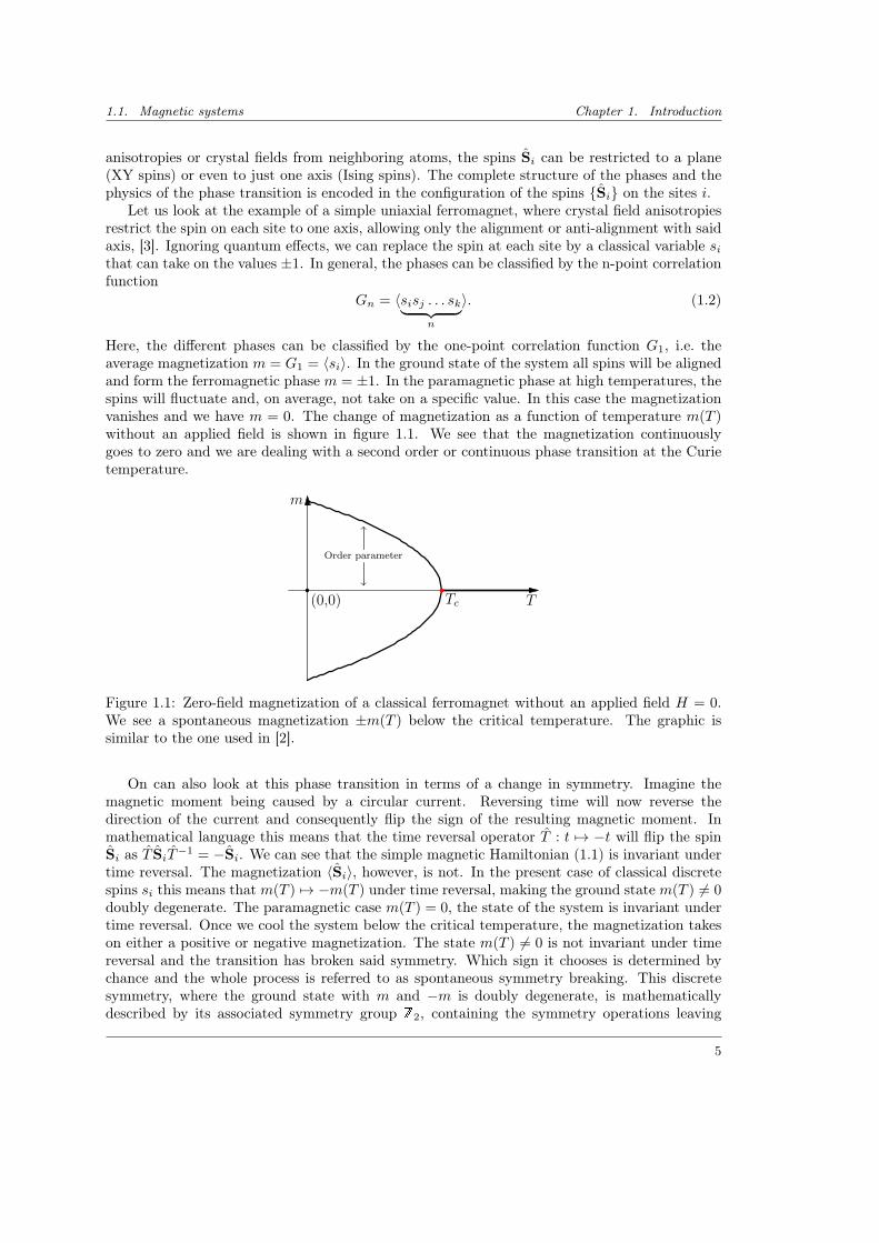
Here, the different phases can be classified by the one-point correlation function G1, i.e. theaverage magnetization m = G1 = 〈si〉. In the ground state of the system all spins will be alignedand form the ferromagnetic phase m = ±1. In the paramagnetic phase at high temperatures, thespins will fluctuate and, on average, not take on a specific value. In this case the magnetizationvanishes and we have m = 0. The change of magnetization as a function of temperature m(T )without an applied field is shown in figure 1.1. We see that the magnetization continuouslygoes to zero and we are dealing with a second order or continuous phase transition at the Curietemperature.

T

m

(0,0) Tc

Order parameter

Figure 1.1: Zero-field magnetization of a classical ferromagnet without an applied field H = 0.We see a spontaneous magnetization ±m(T ) below the critical temperature. The graphic issimilar to the one used in [2].

On can also look at this phase transition in terms of a change in symmetry. Imagine themagnetic moment being caused by a circular current. Reversing time will now reverse thedirection of the current and consequently flip the sign of the resulting magnetic moment. Inmathematical language this means that the time reversal operator T : t 7→ −t will flip the spinSi as T SiT−1 = −Si. We can see that the simple magnetic Hamiltonian (1.1) is invariant undertime reversal. The magnetization 〈Si〉, however, is not. In the present case of classical discretespins si this means that m(T ) 7→ −m(T ) under time reversal, making the ground state m(T ) 6= 0doubly degenerate. The paramagnetic case m(T ) = 0, the state of the system is invariant undertime reversal. Once we cool the system below the critical temperature, the magnetization takeson either a positive or negative magnetization. The state m(T ) 6= 0 is not invariant under timereversal and the transition has broken said symmetry. Which sign it chooses is determined bychance and the whole process is referred to as spontaneous symmetry breaking. This discretesymmetry, where the ground state with m and −m is doubly degenerate, is mathematicallydescribed by its associated symmetry group Z2, containing the symmetry operations leaving

5

Chapter 1. Introduction 1.2. Discrete and continuous symmetry in ferromagnets

the system invariant. Here it consists just of the identity and time reversal operation T . Thebreaking of the symmetry is shown in figure 1.1.

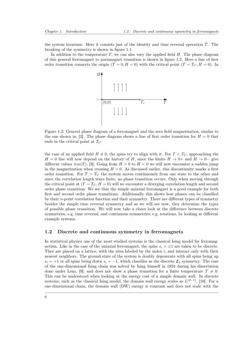
In addition to the temperature T , we can also vary the applied field H. The phase diagramof this general ferromagnet to paramagnet transition is shown in figure 1.2. Here a line of firstorder transition connects the origin (T = 0, H = 0) with the critical point (T = TC , H = 0). In

T

H

(0,0) Tc

Figure 1.2: General phase diagram of a ferromagnet and the zero field magnetization, similar tothe one shown in, [2]. The phase diagram shows a line of first order transition for H = 0 thatends in the critical point at TC .

the case of an applied field H 6= 0, the spins try to align with it. For T < TC , approaching theH = 0 line will now depend on the history of H, since the limits H → 0+ and H → 0− givedifferent values ±m(T ), [3]. Going from H > 0 to H < 0 we will now encounter a sudden jumpin the magnetization when crossing H = 0. As discussed earlier, this discontinuity marks a firstorder transition. For T > TC the system moves continuously from one state to the other andsince the correlation length stays finite, no phase transition occurs. Only when moving throughthe critical point at (T = TC , H = 0) will we encounter a diverging correlation length and secondorder phase transition. We see that the simple uniaxial ferromagnet is a good example for bothfirst and second order phase transitions. Additionally this shows how phases can be classifiedby their n-point correlation function and their symmetry. There are different types of symmetrybesides the simple time reversal symmetry and as we will see now, they determine the typesof possible phase transition. We will now take a closer look at the difference between discretesymmetries, e.g. time reversal, and continuous symmetries, e.g. rotations, by looking at differentexample systems.

1.2 Discrete and continuous symmetry in ferromagnets

In statistical physics one of the most studied systems is the classical Ising model for ferromag-netism. Like in the case of the uniaxial ferromagnet, the spins si = ±1 are taken to be discrete.They are placed on a lattice, with the sites labeled by the index i, and interact only with theirnearest neighbors. The ground state of the system is doubly degenerate with all spins being upsi = +1 or all spins being down si = −1, which classifies as the discrete Z2 symmetry. The caseof the one-dimensional Ising chain was solved by Ising himself in 1924 during his dissertationdone under Lenz, [9], and does not show a phase transition for a finite temperature T 6= 0.This can be understood when looking at the energy cost of a simple domain wall. In discretesystems, such as the classical Ising model, the domain wall energy scales as L(d−1), [10]. For aone-dimensional chain, the domain wall (DW) energy is constant and does not scale with the

6

1.2. Discrete and continuous symmetry in ferromagnets Chapter 1. Introduction

system size. The Ising model without on-site disorder is invariant under translations by multiplesof the lattice constant. The energy of the domain wall is therefore not dependent on its absoluteposition in the chain and once it is created, moving the domain wall does not cost additionalenergy. This freedom in placement of the DW means that the system can increase its entropyand therefore lower its free energy by creating such a wall. The entropy gain is dependent onthe possible positions of the DW and therefor on the system size. In the thermodynamic limitof the one-dimensional system, meaning an infinite chain, the entropy gain S diverges, while theDW energy E is a finite quantity. We can easily see that the free energy

F = E − TS (1.3)

will favor the creation of DW for any temperature T 6= 0. The system stays in the paramagneticphase for all finite temperatures and no phase transition occurs. The situation is different in twodimensions, where the DW energy scales with the system size. Now one has to look exactly attheir scaling to see whether or not there is a finite temperature after which the system will favorDW and destroy any magnetization. Here the system does exhibit ferromagnetic order. Thiswas first proven in 1936 by Peierls, [11]. Taking a fixed array of spins, he introduced boundariespassing between spins with opposite sign, separating the system in open and closed boundaries.Open boundaries start and end on the edges of the arrays, while closed ones encircle a finite areainside the array. He could show that for sufficiently low but finite temperature, the area coveredby these open and closed boundaries is small compared to the system size. The majority of spinsis therefore aligned and the system shows ferromagnetic order, [11]. Later the model was solvedanalytically by Onsager in 1944, [12], showing the existence of a phase transition.

The situation is different for two–dimensional magnetic systems with a continuous symmetrySO(2), such as the classical XY model. They are known to exhibit no true long-range orderfor any finite temperature T > 0, i.e. ferro- or anti- ferromagnetism vanishes in the onset ofthermal fluctuations. In other words, the continuous symmetry of the system cannot be brokenspontaneously in two dimensions. A simple physical explanation for this can be given by energyconsiderations of the domain wall separating different regions of magnetic order. Considering thecontinuously varying magnetization m(x), the energy of the domain wall of a region of size L isgiven by the following term in the Ginzburg–Landau expansion

∫ddx(∇m)2 ∝ Ld−2 scaling, as

shown, as Ld−2 with the general dimension d of the system, [10]. For d = 2 one can see that thesurface energy of the magnetic domain does not increase when expanding the size of the domainitself. The finite domain wall cost is then outweighed by the entropic gain to the system, leadingto the destruction of long-range order. A rigorous proof of this statement has been done byMermin and Wagner in 1966, [10, 13]. On a first glance, one would think that there are no phasetransitions in the simple XY model, with a vanishing magnetization or one-point correlation forany temperature.

However the 2D system with SO(2) symmetry still exhibits a phase transition where quasi–long–range order (QLRO) is established, famously discussed by Berezinskii in 1971, [14], andKosterlitz and Thouless in 1973, [15] now known as the Berezinskii–Kosterlitz–Thouless transition(BKT). The transition is well-understood as the dissociation of topological defects in the spinconfiguration known as vortices, [10]. In this case, the different phases are classified by the two-point correlation function G2 = 〈SiSj〉. Since the BKT mechanism is important later on, we willgo into a little more detail concerning the XY model.

7

Chapter 1. Introduction 1.2. Discrete and continuous symmetry in ferromagnets

The XY model

The XYmodel consists of planar Heisenberg spins Si = (cos(φi), sin(φi), 0) each living on a squarelattice site i. Next neighbors on the lattice are ferromagnetically coupled with K = βJ > 0 as

βHXY = −K∑〈i,j〉

SiSj = −K∑〈i,j〉

cos(φi − φj), (1.4)

where the sum runs over the next-neighbor pairs 〈i, j〉. As discussed in the introduction andknown from the Mermin–Wagner theorem, a 2D system with the presented local interaction andSO(2) symmetry does not exhibit a long range ordered state for a finite temperature T = β−1 > 0.With the average magnetization G1 = 〈Si〉 = 0 for all T 6= 0, it is not suited to classify thedifferent phases. Instead we will use the correlator G2 = 〈S0Sr〉. The position vector r hasbeen used instead of the simple index i for the corresponding lattice site, to illustrate the spatialdependance in the correlator better. A good discussion of the different ordered states in theXY model and the phase transition is discussed in standard textbooks, such as [10]. The shortsummary here will follow [10] closely.

In the low-temperature phase when K 1, fluctuations in the phase difference φi − φj arestrongly suppressed due to their high energy cost. The phases φi will only vary slowly overdistances r a greater than the lattice constant a. In this case, the model can be treated bycontinuum theory. The phase difference is then replaced by the gradient ∇φ(r) with a continuousHamiltonian

βHXY =K

2

∫d2r (∇φ)2 . (1.5)

The fluctuations in the phase are Gaussian. Using Wick’s theorem, [10], the correlator can bewritten as

〈S0Sr〉 = Re〈eı(φ(0)−φ(r))〉 =1

2e−

12 〈(φ(0)−φ(r))2〉 . (1.6)

The fluctuations in 2D are known to be logarithmic with

〈(φ(0)− φ(r))2〉 =1

2πKln

( |r|a

)(1.7)

resulting in a correlator that exhibits algebraic decay of the form

〈S0Sr〉 ≈(a

|r|

) 12πK

(1.8)

This describes the so-called quasi-long-range ordered (QLRO) phase of the system, [10].In the high-temperature case, K → 0, the situation is different. Since K is a small parameter

we can expand the partition function in terms of K as

Z =

∫ 2π

0

∏i

dφi2π

e−βHXY =

∫ 2π

0

∏i

dφi2π

∏〈i,j〉

[1 +K cos(φi − φj) +O(K2)

](1.9)

To lowest order in K, each term in the product is either one or K cos(φi−φj) and can be viewedas a “bond“ connecting neighboring sites i and j, [10]. A single connection or open bond in aconfiguration will vanish since

∫ 2π

0dφ1 cos(φ1 − φ2) = 0. Additionally, we have the relationship∫ 2π

0

dφ2

2πcos(φ1 − φ2) cos(φ2 − φ3) =

1

2cos(φ1 − φ3) (1.10)

8

1.3. Vector and scalar chiral order parameters Chapter 1. Introduction

for two bonds meeting. Only closed loops survive, [10]. Computing the correlation function ofthe system in leading order of K, only closed loops connecting the sites 0 and r will contribute,leading to an exponential decay

〈S0Sr〉 ∼(K

2

)|r|∼ exp

[−|r|ξ

](1.11)

with the correlation length ξ−1 = ln(2/K). Two different phases are present in the XY modelthat can be identified by algebraic and exponential decay of its two-point correlation function.

The transition can be understood by the condensation of vortices in the spin configuration.The low-temperature expansion we used to calculate the algebraic decay in the correlation func-tion deals with continuous deformations in the spin configurations. As we can see in the definitionof HXY the angle is fixed up to an additional constant of 2πn with n being an integer. One cannow construct a configuration where the angle changes by 2πn when choosing a closed path alonga certain point. This configuration cannot be destroyed by continuous deformation and the stateis known to be topologically protected. This defect is known as a vortex and the winding numbern associated with it is referred to as its topological charge, [10]. The energy of the vortex Evconsists of a contribution from the core, which length scale is of the order of the lattice constanta, and the “outside” of the core, resulting in

Ev = Ecore(a) +J

2

∫a

d2r(∇φ)2 = Ecore(a) + πJn2 ln

(L

a

)(1.12)

where the low temperature expansion of the Hamiltonian was used and the definition of a vortexas∮dl (∇φ) = 2πn was used, [10]. Now with a core size of a2 and a system size of L2, there

are L2/a2 possible positions to place the vortex, giving a considerable entropic gain to the freeenergy of the system. Looking at the free energy, kB = 1,

F = E − TS = Ecore + (πJn2 − 2T ) ln

(L

a

), (1.13)

we see that for T < πJ/2 or K > 2/π, the generation of vortices is penalized by the logarith-mically divergent energy cost to the system. In this case the algebraic decay of the spin–spincorrelator is protected. However, for T > πJ/2 the entropic gain outweighs the energy cost ofthe vortex and the spontaneous formation of vortices is favored, destroying the QLRO, [10].

1.3 Vector and scalar chiral order parameters

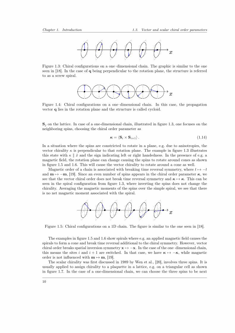
We have seen that the type of symmetry that is broken strongly influences the type of phasetransition that it exhibits. Which begs the question what will happen to the phase transitions ina system where both discrete and continuous symmetries occur simultaneously. In 1959, Villainand Yoshimori simultaneously discussed helimagnets. Here, additionally to the continuous SO(2)symmetry, a discrete Z2 symmetry in form of chiral order is present, [16, 17]. A structure is calledchiral if one cannot map it to its mirror image via simple rotation and translation. For example,your hands are mirror images of each other, that cannot be superposed. As a result of this,we can assign each a “handedness” or chirality by calling them left and right. In the case ofhelimagnets we are dealing with spins in a spiral configuration that can either turn left or right,see figure 1.3.

One generally distinguishes between vector chirality and scalar chirality. The general defini-tion of the vector chiral order parameter as a measure of the canting between two spins Si and

9

Chapter 1. Introduction 1.3. Vector and scalar chiral order parameters

Figure 1.3: Chiral configurations on a one–dimensional chain. The graphic is similar to the oneseen in [18]. In the case of q being perpendicular to the rotation plane, the structure is referredto as a screw spiral.

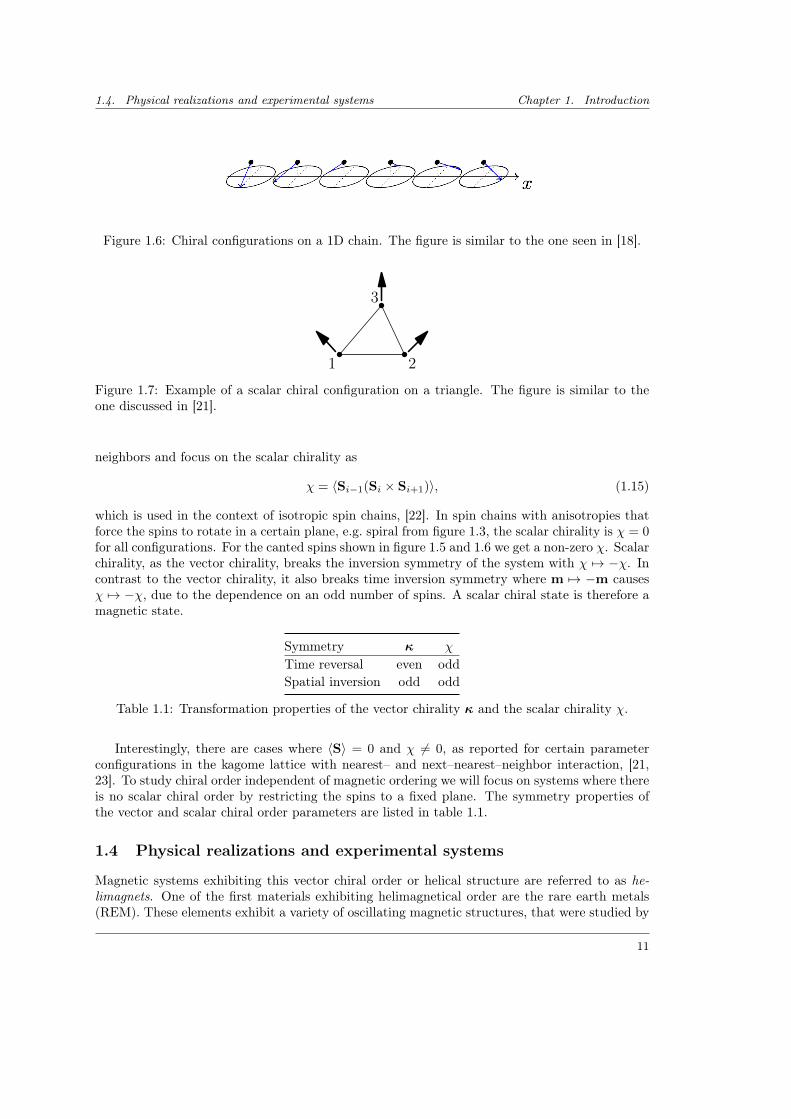
Figure 1.4: Chiral configurations on a one–dimensional chain. In this case, the propagationvector q lies in the rotation plane and the structure is called cycloid.

Sj on the lattice. In case of a one-dimensional chain, illustrated in figure 1.3, one focuses on theneighboring spins, choosing the chiral order parameter as

κ = 〈Si × Si+1〉 . (1.14)

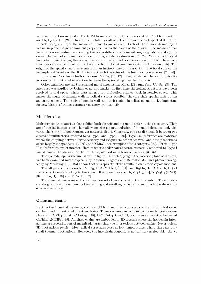
In a situation where the spins are constricted to rotate in a plane, e.g. due to anisotropies, thevector chirality κ is perpendicular to that rotation plane. The example in figure 1.3 illustratesthis state with κ ‖ x and the sign indicating left or right handedness. In the presence of e.g. amagnetic field, the rotation plane can change causing the spins to rotate around cones as shownin figure 1.5 and 1.6. This will cause the vector chirality to rotate around a cone as well.

Magnetic order of a chain is associated with breaking time reversal symmetry, where t 7→ −tand m 7→ −m, [19]. Since an even number of spins appears in the chiral order parameter κ, wesee that the vector chiral order does not break time reversal symmetry and κ 7→ κ. This can beseen in the spiral configuration from figure 1.3, where inverting the spins does not change thechirality. Averaging the magnetic moments of the spins over the simple spiral, we see that thereis no net magnetic moment associated with the spiral.

Figure 1.5: Chiral configurations on a 1D chain. The figure is similar to the one seen in [18].

The examples in figure 1.5 and 1.6 show spirals where e.g. an applied magnetic field causes thespirals to form a cone and break time reversal additional to the chiral symmetry. However, vectorchiral order breaks spatial inversion symmetry x 7→ −x. In the case of the one–dimensional chain,this means the sites i and i + 1 are switched. In that case, we have κ 7→ −κ, while magneticorder is not influenced with m 7→m, [19].

The scalar chirality was first discussed in 1989 by Wen et al., [20], involves three spins. It isusually applied to assign chirality to a plaquette in a lattice, e.g. on a triangular cell as shownin figure 1.7. In the case of a one-dimensional chain, we can choose the three spins to be next

10

1.4. Physical realizations and experimental systems Chapter 1. Introduction

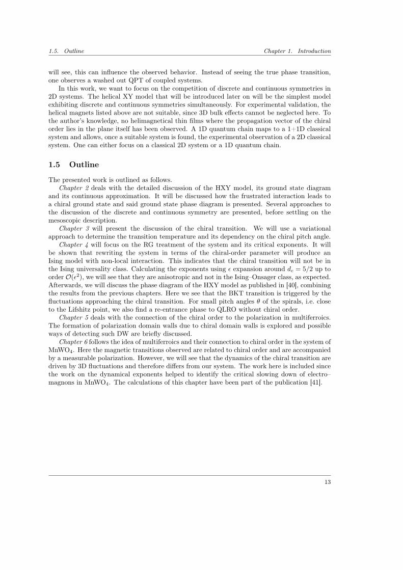
Figure 1.6: Chiral configurations on a 1D chain. The figure is similar to the one seen in [18].

1 2

3

Figure 1.7: Example of a scalar chiral configuration on a triangle. The figure is similar to theone discussed in [21].

neighbors and focus on the scalar chirality as

χ = 〈Si−1(Si × Si+1)〉, (1.15)

which is used in the context of isotropic spin chains, [22]. In spin chains with anisotropies thatforce the spins to rotate in a certain plane, e.g. spiral from figure 1.3, the scalar chirality is χ = 0for all configurations. For the canted spins shown in figure 1.5 and 1.6 we get a non-zero χ. Scalarchirality, as the vector chirality, breaks the inversion symmetry of the system with χ 7→ −χ. Incontrast to the vector chirality, it also breaks time inversion symmetry where m 7→ −m causesχ 7→ −χ, due to the dependence on an odd number of spins. A scalar chiral state is therefore amagnetic state.

Symmetry κ χ

Time reversal even oddSpatial inversion odd odd

Table 1.1: Transformation properties of the vector chirality κ and the scalar chirality χ.

Interestingly, there are cases where 〈S〉 = 0 and χ 6= 0, as reported for certain parameterconfigurations in the kagome lattice with nearest– and next–nearest–neighbor interaction, [21,23]. To study chiral order independent of magnetic ordering we will focus on systems where thereis no scalar chiral order by restricting the spins to a fixed plane. The symmetry properties ofthe vector and scalar chiral order parameters are listed in table 1.1.

1.4 Physical realizations and experimental systems

Magnetic systems exhibiting this vector chiral order or helical structure are referred to as he-limagnets. One of the first materials exhibiting helimagnetical order are the rare earth metals(REM). These elements exhibit a variety of oscillating magnetic structures, that were studied by

11

Chapter 1. Introduction 1.4. Physical realizations and experimental systems

neutron diffraction methods. The REM forming screw or helical order at the Néel temperatureare Tb, Dy and Ho, [24]. These three metals crystallize in the hexagonal closely-packed structure.In each hexagonal layer the magnetic moments are aligned. Each of these monoatomic layershas an in-plane magnetic moment perpendicular to the c-axis of the crystal. The magnetic mo-ment of two succeeding layers along the c-axis differs by a constant angle ϕ0. Moving along thec-axis, the magnetic moments are now forming a helix as shown in 1.3, [24]. With an additionalmagnetic moment along the c-axis, the spins move around a cone as shown in 1.5. These conestructures are stable in holmium (Ho) and erbium (Er) at low temperatures of T ∼ 4K, [25]. Theorigin of the spiral structures stems from an indirect ion–ion interaction. The total spin of theincomplete 4f -shells of the REMs interact with the spins of the free moving electrons, [24, 26].

Villain and Yoshimori both considered MnO2, [16, 17]. They explained the vector chiralityas a result of frustrated interaction between the spins along their heilical axis.

Other examples are the transitional metal silicates like MnSi, [27], and Fe1−xCoxSi, [28]. Thelater case was studied by Uchida et al. and marks the first time the helical structures have beenresolved in real space, where classical neutron-diffraction studies work in Fourier space. Thismakes the study of domain walls in helical systems possible, showing their spatial distributionand arrangement. The study of domain walls and their control in helical magnets is i.a. importantfor new high performing computer memory systems, [29].

Multiferroica

Multiferroics are materials that exhibit both electric and magnetic order at the same time. Theyare of special interest since they allow for electric manipulation of magnetic domains and, viceversa, the control of polarization via magnetic fields. Generally, one can distinguish between twoclasses of multiferroics, referred to as Type I and Type II, [30]. Type I multiferroics are materialswhere the coupling between ferroelectricity and magnetism are rather weak and both phenomenaoccur largely independent. BiFeO3 and YMnO3 are examples of this category, [30]. For us, TypeII multiferroica are of interest. Here magnetic order causes ferroelectricty. Compared to Type Imultiferroics, the strength of the resulting polarization is however weaker, [30–32].

The cycloidal spin structure, shown in figure 1.4, with q lying in the rotation plane of the spin,has been examined microscopically by Katsura, Nagaosa and Balatsky, [33], and phenomenolog-ically by Mostovoy, [19]. Both show that this spin structure results in an electric dipole moment.

The alloys and compounds RMnO3, R ∈ Y,Tb,Dy, [34], and R2Mn2O5, R ∈ Tb, Bi ofthe rare earth metals belong to this class. Other examples are Tb2Mn2O5, [35], Ni3V2O8 (NVO),[34], LiCu2O2, [36] and MnWO4, [37].

These multiferroica make the electric control of magnetic structures possible. Their under-standing is crucial for enhancing the coupling and resulting polarization in order to produce moreeffective materials.

Quantum chains

Next to the “classical” systems, such as REMs or multiferroica, vector chirality or chiral ordercan be found in frustrated quantum chains. These systems are complex compounds. Some exam-ples are LiCuVO4, Rb2Cu2Mo3O12, [38], Li2ZrCuO4, Cs2CuCl4, or the more recently discoveredGd(hfac)3NITiPr, [39]. All these chains are embedded in 3D crystals where the intrachain inter-actions are several orders of magnitude larger then the interactions between chains. Nevertheless,3D fluctuations persist. Most helical structures exist at low temperatures, where there are onlysmall thermal fluctuations. However, the interchain coupling is not entirely neglectable. As we

12

1.5. Outline Chapter 1. Introduction

will see, this can influence the observed behavior. Instead of seeing the true phase transition,one observes a washed out QPT of coupled systems.

In this work, we want to focus on the competition of discrete and continuous symmetries in2D systems. The helical XY model that will be introduced later on will be the simplest modelexhibiting discrete and continuous symmetries simultaneously. For experimental validation, thehelical magnets listed above are not suitable, since 3D bulk effects cannot be neglected here. Tothe author’s knowledge, no helimagnetical thin films where the propagation vector of the chiralorder lies in the plane itself has been observed. A 1D quantum chain maps to a 1+1D classicalsystem and allows, once a suitable system is found, the experimental observation of a 2D classicalsystem. One can either focus on a classical 2D system or a 1D quantum chain.

1.5 Outline

The presented work is outlined as follows.Chapter 2 deals with the detailed discussion of the HXY model, its ground state diagram

and its continuous approximation. It will be discussed how the frustrated interaction leads toa chiral ground state and said ground state phase diagram is presented. Several approaches tothe discussion of the discrete and continuous symmetry are presented, before settling on themesoscopic description.

Chapter 3 will present the discussion of the chiral transition. We will use a variationalapproach to determine the transition temperature and its dependency on the chiral pitch angle.

Chapter 4 will focus on the RG treatment of the system and its critical exponents. It willbe shown that rewriting the system in terms of the chiral-order parameter will produce anIsing model with non-local interaction. This indicates that the chiral transition will not be inthe Ising universality class. Calculating the exponents using ε expansion around dc = 5/2 up toorder O(ε2), we will see that they are anisotropic and not in the Ising–Onsager class, as expected.Afterwards, we will discuss the phase diagram of the HXY model as published in [40], combiningthe results from the previous chapters. Here we see that the BKT transition is triggered by thefluctuations approaching the chiral transition. For small pitch angles θ of the spirals, i.e. closeto the Lifshitz point, we also find a re-entrance phase to QLRO without chiral order.

Chapter 5 deals with the connection of the chiral order to the polarization in multiferroics.The formation of polarization domain walls due to chiral domain walls is explored and possibleways of detecting such DW are briefly discussed.

Chapter 6 follows the idea of multiferroics and their connection to chiral order in the system ofMnWO4. Here the magnetic transitions observed are related to chiral order and are accompaniedby a measurable polarization. However, we will see that the dynamics of the chiral transition aredriven by 3D fluctuations and therefore differs from our system. The work here is included sincethe work on the dynamical exponents helped to identify the critical slowing down of electro–magnons in MnWO4. The calculations of this chapter have been part of the publication [41].

13

2. The Model

The easiest model containing both the Z2 and SO(2) symmetry is the classical helical XY model(HXY). The system is archetypical for frustrated systems with these two types of symmetries.Compared to more complicated models, it has the advantage of being accessible by an analyticalapproach. It is essentially the XY model with an additional frustration introduced in the xdirection that produces a helical ground state along that direction. The XY model itself has aprominent place in physics for exhibiting a phase transition driven by topological excitations,i.e. vortices, named after their discoverers as Berezinskii–Kosterlitz–Thouless (BKT) transition,[14, 15]. After the model and its frustrated interaction have been introduced, we will focus onits ground state properties and the symmetries of the phase diagram. Moving to scales largerthan the microscopic lattice spacing a but still smaller than the pitch angle of the helical screwsθ (a x θ−1) we can describe the angles φi of the spins as continuous functions φ(x). Thismesoscopic model will be quite useful later on.

A different microscopic approach starts with a one–dimensional frustrated quantum chains.Quantum-mechanical systems in d dimensions are connected to (d + 1)-dimensional classicalsystems via the path-integral formalism, [42]. The mapping to a quantum system is useful whentrying to find experimental realizations of our model to test the theoretical predictions. A directmapping of a frustrated quantum chain to the mesoscopic version of the HXY model has beenworked out by Kolezhuk, [43], and will be discussed later in this chapter. In the case of largespins, quantum fluctuations can be ignored, [10], and the discussion of the one–dimensionalquantum chain and the classical two–dimensional HXY model are identical for small pitch anglesθ of the helix.

The study of the competing symmetries Z2 and SO(2) can also be approached from a macro-scopic point of view, using the Ginzburg–Landau theory of phase transitions. The GL-free energyfor these types of systems can be derived by symmetry considerations using group theory, as doneby Bak and Mukamel for several different crystal symmetry groups, [44], or by starting from themicroscopic model doing an expansion around the critical modes, as done by Kawamura, [45].We will discuss the GL–theory at the end of this chapter.

2.1 The classical model

In this section, we will expand the XY model by introducing an additional discrete symme-try through frustration, which leads to the helical XY model. We start from the discrete 2DXY model with planar Heisenberg spins Si = (cos(φi), sin(φi), 0). The ferromagnetic nearest–neighbor (NN) interaction is different in the x-direction (K0) from the one in the y-direction (K1).Then we introduce the frustration via an anti–ferromagnetic next–nearest–neighbor (NNN) in-teraction in the x-direction to produce the general HXY model as

−βHHXY =∑i

(K0SiSi+x +K1SiSi+y +K2SiSi+2x)

=∑i

(K0 cos(φi − φi+x) +K1 cos(φi − φi+y) +K2 cos(φi − φi+2x)) (2.1)

with the inverse temperature β = 1/kBT and the interaction parameters Kn = βJn. The indexi running over all sites of a 2D square lattice. The system in y direction is a simple NN spin

15

Chapter 2. The Model 2.1. The classical model

chain with a ferromagnetic (K1 > 0) or anti-ferromagnetic (K1 < 0) ground state.

Ground state

Let us take a closer look at the ground state properties of the system. The interaction iny-direction forces the spins to be either aligned (K1 > 0) or anti-aligned (K1 < 0) in thatdirection. The situation is not that simple in the x-direction. For the classical ground state, wecan just focus on the classical linear chain in x-direction, given by

Hx = −∑i

(J0 cos(φi − φi+1) + J2 cos(φi − φi+2)) . (2.2)

In the case for J0 > 0 and J2 > 0, both interactions are ferromagnetic and force all the spins tobe aligned in the ground state. The first quadrant of the ground state phase diagram in J2−J1 istherefor in the ferromagnetic phase (FM). Changing the NN interaction to be anti–ferromagnetic,J0 < 0, while keeping the NNN interaction ferromagnetic, J2 > 0, the system favors anti–alignment in the ground state. The 4th quadrant of the ground state phase diagram is thereforecompletely located in the anti-ferromagnetic phase (AFM). The interesting effects are causedby the frustrated interaction in the x-direction, when NN is ferromagnetic J0 > 0 and NNNanti–ferromagnetic J2 < 0, or both are anti–ferromagnetic. In these cases the system can exhibitan additional chiral ground state depending on the parameter ratio k = −J0/4J2 = −K0/4K2,which was shown by Villain and Yoshimori, [16, 17].

Let us introduce the chiral angle θ = φi − φi+1 as the difference between neighboring spin-angles. In the spiral case, θ is independent of the lattice site and θ = const. Now, we can writethe energy per site EN = H/N of the one–dimensional chain from equation 2.2 as

EN = −J0 cos(θ)− J2 cos(2θ). (2.3)

Computing the derivative, we obtain the following condition for the minimum

∂θEN = sin(θ) (J0 + 4J2 cos(θ))!= 0, (2.4)

which has three different solution. We have the ferromagnetic (FM) ground state with θ = 0 andthe anti–ferromagnetic (AFM) ground state with θ = π both follow from sin(θ) = 0. By settingthe second factor to zero we get the chiral (Ch) ground state with

cos(θ) = − J0

4J2≡ k (2.5)

θ = arccos

(− J0

4J2

)(2.6)

as e.g. shown in [46]. Parameter configurations for J0 and J2 with |k| > 1 have no chiralstructure. The ferromagnetic phase will therefore extend up to the critical line J0 = −4J2. Theanti–ferromagnetic phase will be limited by J0 = 4J2. In the parameter regime of −1 ≤ k ≤ 1,we have to compare the energies of the different phases in order to decide which one is chosenby the system. At the line J0 = −4J2, where k = 1 and θ = 0 the energies for both phases areidentical to the FM phase with

EN (θ = 0) = −|J0|+ |J2|. (2.7)

Now decreasing J2 or increasing |J2| leads to k < 1 and θ > 0. Comparing the energy for a smallθ to its FM alternative we have

EN (θ) = −|J0| cos(θ) + |J2| cos(2θ) ≈ EN (θ = 0) + 2θ2(|J0| − 4|J2|) +O(θ4). (2.8)

16

2.1. The classical model Chapter 2. The Model

The last term can be written in terms of the parameter k. The difference in energy then is

EN (θ)− EN (θ = 0) ≈ 2θ2|J0|(

1− 1

|k|

). (2.9)

For |k| < 1 the difference is always negative and the chiral state is chosen. The argument for theAFM phase, where one expands around θ = π leads to the same expression.

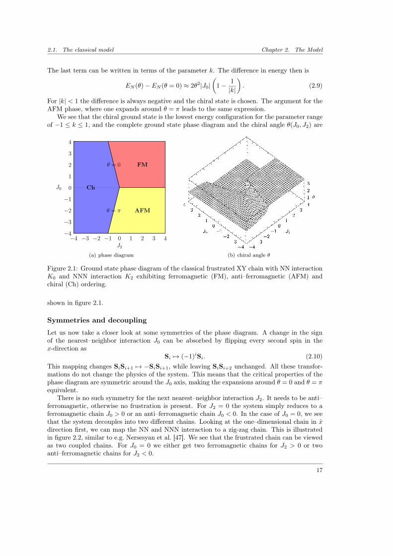
We see that the chiral ground state is the lowest energy configuration for the parameter rangeof −1 ≤ k ≤ 1, and the complete ground state phase diagram and the chiral angle θ(J0, J2) are

−4

−3

−2

−1

0

1

2

3

4

J0

−4 −3 −2 −1 0 1 2 3 4J2

Ch

FM

AFM

θ = 0

θ = π

(a) phase diagram (b) chiral angle θ

Figure 2.1: Ground state phase diagram of the classical frustrated XY chain with NN interactionK0 and NNN interaction K2 exhibiting ferromagnetic (FM), anti–ferromagnetic (AFM) andchiral (Ch) ordering.

shown in figure 2.1.

Symmetries and decoupling

Let us now take a closer look at some symmetries of the phase diagram. A change in the signof the nearest–neighbor interaction J0 can be absorbed by flipping every second spin in thex-direction as

Si 7→ (−1)iSi. (2.10)This mapping changes SiSi+1 7→ −SiSi+1, while leaving SiSi+2 unchanged. All these transfor-mations do not change the physics of the system. This means that the critical properties of thephase diagram are symmetric around the J0 axis, making the expansions around θ = 0 and θ = πequivalent.

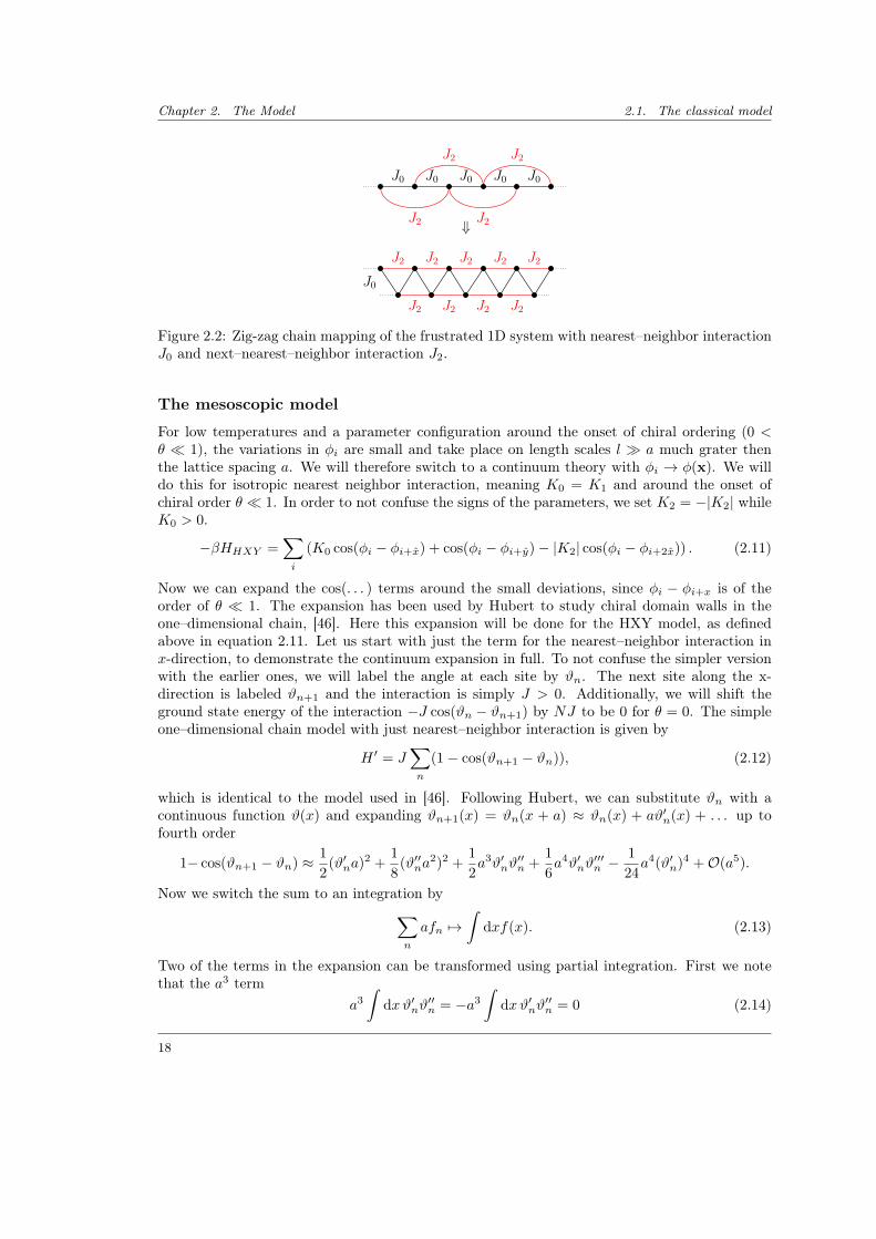
There is no such symmetry for the next nearest–neighbor interaction J2. It needs to be anti–ferromagnetic, otherwise no frustration is present. For J2 = 0 the system simply reduces to aferromagnetic chain J0 > 0 or an anti–ferromagnetic chain J0 < 0. In the case of J0 = 0, we seethat the system decouples into two different chains. Looking at the one–dimensional chain in xdirection first, we can map the NN and NNN interaction to a zig-zag chain. This is illustratedin figure 2.2, similar to e.g. Nersesyan et al. [47]. We see that the frustrated chain can be viewedas two coupled chains. For J0 = 0 we either get two ferromagnetic chains for J2 > 0 or twoanti–ferromagnetic chains for J2 < 0.

17

Chapter 2. The Model 2.1. The classical model

J2 J2

J2 J2

J0 J0 J0 J0 J0

⇓

J2 J2 J2 J2 J2

J2 J2 J2 J2

J0

Figure 2.2: Zig-zag chain mapping of the frustrated 1D system with nearest–neighbor interactionJ0 and next–nearest–neighbor interaction J2.

The mesoscopic model

For low temperatures and a parameter configuration around the onset of chiral ordering (0 <θ 1), the variations in φi are small and take place on length scales l a much grater thenthe lattice spacing a. We will therefore switch to a continuum theory with φi → φ(x). We willdo this for isotropic nearest neighbor interaction, meaning K0 = K1 and around the onset ofchiral order θ 1. In order to not confuse the signs of the parameters, we set K2 = −|K2| whileK0 > 0.

−βHHXY =∑i

(K0 cos(φi − φi+x) + cos(φi − φi+y)− |K2| cos(φi − φi+2x)) . (2.11)

Now we can expand the cos(. . . ) terms around the small deviations, since φi − φi+x is of theorder of θ 1. The expansion has been used by Hubert to study chiral domain walls in theone–dimensional chain, [46]. Here this expansion will be done for the HXY model, as definedabove in equation 2.11. Let us start with just the term for the nearest–neighbor interaction inx-direction, to demonstrate the continuum expansion in full. To not confuse the simpler versionwith the earlier ones, we will label the angle at each site by ϑn. The next site along the x-direction is labeled ϑn+1 and the interaction is simply J > 0. Additionally, we will shift theground state energy of the interaction −J cos(ϑn − ϑn+1) by NJ to be 0 for θ = 0. The simpleone–dimensional chain model with just nearest–neighbor interaction is given by

H ′ = J∑n

(1− cos(ϑn+1 − ϑn)), (2.12)

which is identical to the model used in [46]. Following Hubert, we can substitute ϑn with acontinuous function ϑ(x) and expanding ϑn+1(x) = ϑn(x + a) ≈ ϑn(x) + aϑ′n(x) + . . . up tofourth order

1− cos(ϑn+1 − ϑn) ≈ 1

2(ϑ′na)2 +

1

8(ϑ′′na

2)2 +1

2a3ϑ′nϑ

′′n +

1

6a4ϑ′nϑ

′′′n −

1

24a4(ϑ′n)4 +O(a5).

Now we switch the sum to an integration by∑n

afn 7→∫

dxf(x). (2.13)

Two of the terms in the expansion can be transformed using partial integration. First we notethat the a3 term

a3

∫dxϑ′nϑ

′′n = −a3

∫dxϑ′nϑ

′′n = 0 (2.14)

18

2.1. The classical model Chapter 2. The Model

vanishes. Secondly, we will simplify the ϑ′ϑ′′′ term as

a4

6

∫dxϑ′nϑ

′′′n = −a

4

6

∫dx (ϑ′′n)2. (2.15)

With this, the simple model H ′ of equation (2.12) can be written as

H ′ =Ja

2

∫x

[(∂xϑ)2 − a2

12

((∂2xϑ)2 + (∂xϑ)4

)].

Since we will consider a two–dimensional system in the end, let us assume a second index jrunning in the y-direction, that can be transformed into a continuous variable y. Instead of ϑnwe now have ϑn,j , with the sum running over both indices

∑n,j . The additional constant a in

front can then be used for switching a∑j 7→

∫dy, leading to

H ′ =J

2

∫x,y

[(ϑ′)2 − a2

12

((ϑ′′)2 + (ϑ′)4

)](2.16)

with ϑ ≡ ϑ(x) and the prime denoting the derivative in x, analog to [46]. This is without anyinteraction in the y-direction. There is only a nearest–neighbor interaction in the y-direction,resulting in a simple coupling without the emergence of chiral order. It is not necessary to expandthe cos(. . . ) term beyond the quadratic terms. An isotropic NN interaction (K0 = K1 = J)then just adds a (∂yϑ(x))2 term to the expansion. Writing the derivatives as subindices, i.e.∂x/yϑ ≡ ϑx/y, we have

H ′ =K0

2

∫x,y

[(ϑx)2 + (ϑy)2 − a2

12

((ϑxx)2 + (ϑx)4

)]. (2.17)

In order to obtain the continuum expansion for the NNN contribution K2, we have to expandcos(ϑn+2 − ϑn) as

1− cos(ϑn+2 − ϑn) ≈ 2(ϑ′na)2 + 2(ϑ′′na2)2 + 4a3ϑ′nϑ

′′n +

8

3a4ϑ′nϑ

′′′n −

2

3a4(ϑ′n)4 +O(a5).

Using partial integration we can simplify these terms again. The continuum version of just theNNN part of the expansion yields

H ′′ = −|K2|2

∫x,y

[4(ϑx)2 − 16a2

12

((ϑxx)2 + (ϑx)4

)]. (2.18)

Now we can combine all the calculations and switch back to the notation using φ(x) for theangle of a spin at position x.

βH ≈ 1

2

∫d2x

[(K0 − 4|K2|)(∂xφ)2 − a2

12(K0 − 16|K2|)

((∂2xφ)2 + (∂xφ)4

)+K0(∂yφ)2

]+ const

Factoring out K0 and using cos(θ) = K0/(4|K2|) we get

βH ≈ K0

2

∫d2x

[(1− 1

cos(θ)

)(∂xφ)2 − a2

12

(1− 4

cos(θ)

)((∂2xφ)2 + (∂xφ)4

)+ (∂yφ)2

]+ const

This can now be expanded around small θ.

βH ≈ K0

2

∫d2x

[−θ

2

2(∂xφ)2 +

1

4

((∂2xφ)2 + (∂xφ)4

)+ (∂yφ)2

], (2.19)

19

Chapter 2. The Model 2.2. Quantum chain

where we set a = 1 to simplify the notation. This continuous version of the model will be usedthroughout the work. Shifting the ground state energy again by adding −K0

2

∫d2x 1

4θ4 we get

βH =K0

2

∫x

[1

4((∂xφ)2 − θ2)2 + (∂yφ)2 +

1

4(∂2xφ)2

](2.20)

with the chiral or pitch angle θ = qa and∫x

=∫

dxdy. In this version the double minimum∂xφ = ±θ of the Hamiltonian is clearly visible. This model will mainly be used throughout thework.

2.2 Quantum chain

Now we have seen how chiral order can originate from frustrated interaction. For a fixed pa-rameter configuration we have two different chiral ground states with ±θ. This vector chiralityis another example of the Z2 symmetry. Now let us look at one–dimensional quantum chains.We already mentioned the general connection of d–dimensional quantum systems to (d + 1)–dimensional classical systems and here we want the discuss the corresponding quantum model tothe previously discussed classical one. The quantum version is the frustrated one–dimensionalXY quantum chain which is given by

−βH =∑i

K0SiSi+1 +K2SiSi+2 (2.21)

Here we used the inverse temperature β and the interaction parameters Ki = βJi, identical tothe previous discussions. A good introduction into quantum spin chains can be found in [42].

Symmetries

Let us begin with simple symmetry considerations. Since we are dealing with operators insteadof classical spins, we have to check if the classical transformations used are still applicable. Thespin operators Si = (Sxi , S

yi , 0) obey the commutator relations

[Sαi , Sβj ] = ıδijεαβγ S

γi . (2.22)

For K2 = 0 we are dealing purely with the nearest–neighbor interaction K0 leading to a ferro-magnetic chain in the case of K0 > 0 and an anti–ferromagnetic chain for K0 < 0. For classicalspins Si we already discussed that one can map the ferromagnetic K0 to the anti–ferromagneticcase −K0 by flipping every second spin, i.e.

Si 7→ (−1)iSi (2.23)

leading to the term SiSi+1 7→ −SiSi+1 to pick up a minus sign, while next–nearest–neighbor in-teractions are unchanged with SiSi+2 7→ SiSi+2. The situation is more complicated for quantumchains. Inverting all spin components Sx, Sy and Sz on a sub–lattice violates the commutator re-lations. However it is possible to flip only two components of the spin, equivalent to a 180-degreerotation around the axis of the third component, being

Sxi 7→ Sxi = (−1)iSxi ,

Syi 7→ Syi = (−1)iSyi ,

Szi 7→ Szi = Szi .

20

2.2. Quantum chain Chapter 2. The Model

When looking at the nearest–neighbor interaction for Heisenberg spins

SiSi+1 = Sxi Sxi+1 + Syi S

yi+1 + Szi S

zi+1

=1

2(S+i S−i+1 + S−i S

+i+1) + Szi S

zi+1 (2.24)

with S±i = Sxi ± ıSyi , we see that our transformation will flip the sign in front of the Sx/yi Sx/yi+1

terms but leave the Szi Szi+1 part unchanged. In the case of Heisenberg spins there is a differencefor ferromagnetic and anti–ferromagnetic interactions, resulting in different dispersion relationsfor their spin wave excitations. The excitations in the FM Heisenberg chain behave like freeparticles with ω ∼ k2 while the excitations in the AFM Heisenberg chain behave like phononswith ω ∼ k, [10, 42, 48]. In the special case of XY spins, the Sz component does not appear inthe Hamiltonian. Here the 180 rotation can absorb the changed sign in K0 and the quantumsystem has the same symmetry aroundK0 as the classical version discussed earlier. The quantumXY chain with only NN interaction produces a linear dispersion relation ω ∼ k in both theferromagnetic and anti–ferromagnetic case. A detailed discussion and calculation including theexactly solvable S = 1/2 case and the S 1 limit can be found in appendix A.1.

Kolezhuk mapping

For low temperatures, the 1D quantum system can be mapped to a 1+1D classical system wherethe spatial extension of the system along the imaginary time axis τ is

Lτ =~kbT

(2.25)

[42]. For zero temperature the system maps then to a fully 2D classical theory when Lτ → ∞.The HXY is essentially the XY model with an additional frustration in the x direction analogto Villain’s model. For small pitch angles θ of the chiral states, a full winding takes place over adistance l a much larger than the lattice constant. In that case we can move to a continuousφi 7→ φ(x, y) theory of the spin angles. In the case of isotropic NN interaction, i.e. K0 = K1,the resulting mesoscopic model (a = 1) was derived as

βH =K0

2

∫x

[1

4((∂xφ)2 − θ2)2 + (∂yφ)2 +

1

4(∂2xφ)2

]; (2.26)

The derivation was done earlier by substituting φi 7→ φ(x, y) and φi+x 7→ φ(x + a, y) andexpanding the difference φi − φi+x in the cos(. . . ) terms, similar to the expansion proposed byHubert [46].

In the case of the frustrated XY chain for large spin, Kolezhuk [43] was able to map thesystem to a classical helimagnet with the action

A[ϕ] =1

2Teff

∫dx

∫dy

[1

4((∂xϕ)2 − θ2)2 + (∂yϕ)2 +

1

4(∂2xϕ)2

], (2.27)

where effective temperature Teff is related to the spin S via Teff =√

32

1S , relating to the value

K0 used in our definition as

K0 =

√2

3S. (2.28)

Even though we will be dealing with a purely classical system, this relation can be used to connectit to the large spin case of frustrated 1D quantum chains, [43]. The procedure is sketched out inmore detail in the appendix A.2.

21

Chapter 2. The Model 2.3. Landau–Ginzburg–Wilson Hamiltonian

2.3 Landau–Ginzburg–Wilson Hamiltonian

A different approach to the chiral systems has been done by Bak and Mukamel, [44], usingsymmetry considerations to construct the Landau–Ginzburg–Wilson (LGW) Hamiltonian. Fora system with a chiral wave vector q in one direction, they constructed a 4-component order-parameter expansion. This model connects to the models we have discussed so far. A derivationstarting from a microscopic model, followed by an expansion around its critical modes, wasdone by Kawamura, [49, 50], and leads to the same Hamiltonian. Both, the work done by Bakand Mukamel and the work done by Kawamura consider 3D systems. The derivation can beeasily modified to suit the 2D case, but there are several disadvantages that make further studyimpractical. The critical dimension for the LGW system is dc = 4, making a renormalization-group approach for d = 2 impossible. Also, we will see that splitting the order parameters intoa right and left spiral state will be helpful. The coupling of these two different states will turnout to not be small in the chiral regime that we want to study. Both points render this line ofattack on the problem unfruitful. The works are discussed here nevertheless, to give a sense ofthese approaches.

Bak and Mukamel approach

Let us start with the purely macroscopic approach used by Bak and Mukamel, [44]. Theyconsider the spiral structures that emerge in the rare earth metals Ho, Tb and Dy, by lookingat their underlying crystal symmetry. As mentioned in the introduction, they crystallize in thehexagonal closely-packed structure and in each hexagonal layer, their magnetic moments arealigned. Moving along the z-axis, perpendicular to the different layers, the magnetic momentsform a helix, described by the wave vector q = (0, 0, θ/a). As order parameter, they choose theFourier coefficients of the magnetic moments around the wave vector q of the chiral configuration,given as

ψ±q,P = φP ± ıφP =∑r

SP (r)e±ıqr, P = x, y. (2.29)

In the case of a chiral structure around the z-axis, the wave vector is given by q = (0, 0, q) =(0, 0, θ/a), with XY spins S = (Sx, Sy, 0) in the plane perpendicular to q. Writing down thesymmetry invariants of these order parameters, Bak and Mukamel arrive at the following LGW-expansion

HBM =1

2

[((∇φx)2 + (∇φy)2 + (∇φx)2 + (∇φy)2 + r(φ2

x + φ2y + φ2

x + φ2y)]

+ u1(φ2x + φ2

y + φ2x + φ2

y)2 + u2(φxφy − φyφx)2 (2.30)

The gradient terms favor a homogeneous order parameter. The parameters r, u1 and u2 nowdetermine the minimum configuration of the system. In the simple case when all of them arepositive, the minimum is reached when all four order parameters vanish. For different parameterconfigurations, the order parameter can take on finite values, marking ferromagnetic or chiralstructures. In the present notation, the system is not very transparent. A better understandingof this expansion can be obtained by introducing the parameters ηi and ηi

η1 =1√2

(φx + φy), η2 =1√2

(φx − φy), (2.31)

η1 =1√2

(φx − φy), η2 =1√2

(φx + φy). (2.32)

22

2.3. Landau–Ginzburg–Wilson Hamiltonian Chapter 2. The Model

in order to identify the left and right twisting spiral configurations. The describe the spiral partsof the magnetic structure as

η1,2 ∝∑r

Sx(r) cos(kr)± Sy(r) sin(kr), (2.33)

η1,2 ∝∑r

±Sx(r) cos(kr) + Sy(r) sin(kr), (2.34)

[44]. Grouping the parameters corresponding to the different chiralities

ηi =

(ηiηi

)(2.35)

now makes the discussion clearer. Here η1 corresponding to the right-handed spiral and η2

corresponding to the left-handed case. The free energy now has the form

F =1

2r∑i

η2i + 4u′

(∑i

η2i

)2

+ 8u′η21η

22

=1

2r[η2

1 + η22

]+ u

[(η2

1

)2+(η2

2

)2]+ 2v η2

1η22. (2.36)

The coefficients u and v are related to the previous coefficients u1 and u2 via

u = u1 −1

4u2, v =

1

2u2. (2.37)

Ground state

In its form given in equation (2.36), the structure becomes clear. For r < 0 and u > 0, the systemwill favor non vanishing amplitudes |ηi| for the left- and right-handed chiral structures. Nowthe coupling parameter v determines if they both exist simultaneously and form a ferromagnetic(FM) structure or if only one is favored, describing a chiral state (Ch). For r > 0 and u > 0both amplitudes vanish and the system is paramagnetic (P). These configurations are listed intable 2.1. Some special cases can be discussed before doing a direct minimization of the energy.

P Ch+ Ch- FM|η1| 0 const 0 const|η2| 0 0 const const

Table 2.1: Overview of the possible ground states. P being the paramagnetic state, Ch+ and Ch-corresponding to the right or left chiral structure and FM being the ferromagnetic configuration

Without a coupling between the two amplitudes, v = 0, we are dealing with two independent two-component systems. Both having the exact same structure and are determined by the parametersr and u, meaning that they will simultaneously be either 0 or non-vanishing. In the case of r < 0and u > 0, the system will be in the FM state, since both amplitudes will not vanish. In thespecial case of v = u, the whole system can be written in terms of the 4-component vectorg = η1 ⊕ η2, with

F =1

2rg2 + u(g)4.

23

Chapter 2. The Model 2.3. Landau–Ginzburg–Wilson Hamiltonian

The system only fixes the amplitude of g and is invariant under rotation. For a fixed amplitudethe direction (1, 0, 0, 0), referring to |η1| 6= 0 and |η2| = 0, has the same energy as the direction1√2(1, 0, 1, 0), referring to both amplitudes being non-vanishing. The line u = v therefore marks

the transition from a ferromagnetic to a chiral state, because both will have the same energy forthis parameter configuration.

Let us now exactly calculate the minimum of the energy. Minimizing the gradient terms isdone by having spatially constant order parameters. The energy is then simply given as

E =1

2r[η2

1 + η22

]+ u

[(η2

1)2 + (η22)2]

+ 2vη21η

22 (2.38)

and the minimum is determined by

∂ηx/y1E = rη

x/y1 + 4u(η

x/y1 )3 + 4uη

x/y1 (η

y/x1 )2 + 4vη

x/y1 ((η

x/y2 )2 + (η

y/x2 )2) = 0. (2.39)

The different possible solutions and their respective energies for r < 0 can now be calculated.

P |η1| = |η2| = 0 E = 0 (2.40)

Ch |η1| =√− r

4u; η2 = 0 E = − 1

16

r2

uu > 0 (2.41)

FM |η1| = |η2| =√ −r

4(u+ v)E = −1

8

r2

(u+ v)u+ v > 0 (2.42)

We see that the energy is not bounded from below for u < 0 and v < −u, and the system isunstable for those parameter configurations. The full mean-field phase diagram of the systemis shown in figure 2.3. One can see that around v ≈ 0, where the two chiralities η1/2 decouple,

v

u

unstable v = 0

v = 2u

v = u

v = −u

Ch

FM

(0,0)

Figure 2.3: Mean-field solutions for the free energy expansion of the system.

the system is in the ferromagnetic state. In the chiral case that we are interested in, none of theparameters can be treated as a perturbation.

Kawamura expansion

The Landau–Ginzburg–Wilson (LGW) expansion of the microscopic HXY model has been stud-ied by Kawamura in 1988, [49, 50], to calculate the critical behavior in 3D using the renormalization-group. Starting from the microscopic hard-spin model, using the Fourier transform and keeping

24

2.3. Landau–Ginzburg–Wilson Hamiltonian Chapter 2. The Model

only near-critical modes, the effective system reads as

HLGW =1

2

[(∇a)2 + (∇b)2 + r(a2 + b2) + u(a2 + b2)2 + v(ab)2 − a2b2

], (2.43)

where a and b are the 2-component vector fields corresponding to the sine and cosine componentsof the non-collinear spin structure with the wave vector q, [49, 50].

〈S(r)〉 = a(r) cos(qr) + b(r) sin(qr). (2.44)

We see that the system favors a ⊥ b for v > 0, corresponding to the spiral structure. In thecase of v < 0 the vectors a and b tend to align and form linear polarized spin structure, [49].The expansion derived from the microscopic model by Kawamura is actually identical to the onederived simply by symmetry considerations done by Bak and Mukamel. Looking at the nearcritical modes around q we see the immediate connection between the order parameters used byBak and Mukamel and the order parameter used by Kawamura, being

φx/y ∼ ax/y, φx/y ∼ bx/y. (2.45)

The first three terms in the expansion by Bak and Mukamel, equation 2.30, can be easily rec-ognized as being equal to the first three of the Kawamura expansion in equation 2.43 using theidentified connection of the order parameters from equation 2.45. The last term can be checkedby computing

(ab)2 − a2b2 = a2xb

2x + 2axbxayby + a2

yb2y − a2

xb2x − a2

xb2y − a2

yb2x − a2

yb2y = −(axby − aybx)2 (2.46)

and again using the identification ax/y ↔ φx/y and bx/y ↔ φx/y from equation 2.45. Theparameters are connected via

r = r, u1 =1

2u, u2 = −1

2v, (2.47)

r = r, u =1

2u+

1

8v, v = −1

4v. (2.48)

The connection to the microscopic parameters J0, J1, J2 has been formally calculated by Kawa-mura, [45, 49], as

r =1

c1

(1

2Pii −

1

4+ c0

), u =

3

256

1

c21, v =

1

64c21, (2.49)

where the the matrix P is given in relation to the interaction matrix of the HXY system writtenas H =

∑ij SiKijSj with

Kij = J0δi,i+x + J1δi,i+y + J2δi,i+2x. (2.50)

The matrix P is now the inverse defined as

Pij = [P0δij +Kij ]−1, (2.51)

where the constant P0 is chosen to make P positive definite. The constants c0 and c1 are thecoefficients of the expansion of the Fourier transform P (q) of P

P (q) ≈ c0 + c1q2 +O(q4), (2.52)

[45, 49]. However, the elements Pii and the coefficients c0 and c1 are never explicitly calculated.The calculation does not give explicit values for the microscopically determined coefficients r, uand v, but still connects the symmetry considerations to a microscopic model where the chiralityis driven by frustrated interaction.

25

3. Chiral Transition

In this chapter we will focus on the chiral transition of the HXY model. The starting point isits continuous version, the Hamiltonian H

βH =K0

2

∫d2x

[1

4

[(∂xφ)2 − θ2

]2+ (∂yφ)2 +

1

4(∂2xφ)2

](3.1)

which we discussed in chapter 2. The potential for the ∂xφ terms has the form of a double wellwith the two minima at ∂xφ = ±θ. The term (∂xφ)4 complicates the system, a straight for-ward computation of the partition function and the thermodynamical properties is not possible.Instead we will approximate the system with a quadratic trial Hamiltonian HT .

βHT =K0

2

∫d2x

[r((∂xφ)−Q)2 + (∂yφ)2 +

1

4(∂2xφ)2

](3.2)

with the parameters r and Q. The quadratic nature of HT will make analytic computationspossible. Now we have to find the optimal values for r and Q for a given K0, such that theapproximation is closest to the original. So what is meant by “closest” approximation and howcan the quality of the approximation be measured? This is done by constructing a functional withcertain properties, whose minimum is determined by the original Hamiltonian. This so calledvariational approach is used in order to determine the best possible parameters approximatingthe original system, [51].

3.1 The variational approach

We will start by constructing the above mentioned functional V[HT ]. All thermodynamic prop-erties of the system are encoded in its thermodynamical potential, the free energy

F = −T ln(Z) (3.3)

and the partition function Z of the system. The partition functions of the system are given by

Z =

∫D[φ]e−βH ZT =

∫D[φ]e−βHT

where the integration∫D[φ] is over all field configurations. Starting from the partition function

of the original system, we can insert 0 = βHT − βHT without changing the result

Z =

∫D[φ]e−βH =

∫D[φ]e−βH+βHT−βHT (3.4)

By multiplying the expression with 1 = ZT /ZT , we can define the average 〈. . . 〉T

〈. . . 〉T =1

ZT

∫D[φ]e−βHT (. . . ) (3.5)

in the expression. The partition function Z can now be written as the averaged function of thedifference between the original and the trial Hamiltonian.

Z = ZT

⟨e−β(H−HT )

⟩T

(3.6)

27

Chapter 3. Chiral Transition 3.1. The variational approach

In order to compute the average of a function exp(. . . ), we would need to compute the averageof all powers of the argument. This is not feasible. But it is possible put a lower limit on thepartition function using Jensens inequality 〈e−A〉 ≥ e−〈A〉, [51].

Z ≥ ZT e〈−β(H−HT )〉T (3.7)

Taking the logarithm on both sides we get

− ln(Z) ≤ − ln(ZT ) + 〈βH − βHT 〉T

So the minimum of the functional

V[HT ] = − ln(ZT ) + 〈βH − βHT 〉T != min (3.8)

now determines the best or “closest” approximation of the system.

Computing the derivatives

The minimum condition ∂αV != 0 now determines the optimal parameters α = r,Q. The

calculation is done in two parts. First the equation is reduced to simple averages which will beevaluated in the second part.

Reducing the minimum condition to simple averages

Starting with the first term lnZT from equation (3.8) we immediately get

−∂α ln(ZT ) = − 1

ZT

∫D[φ]e−βHT (∂α(−βHT )) = 〈(∂αβHT )〉T (3.9)

This reduces the problem to the simple average of the derivatives of the trial Hamiltonain. Whendealing with the second part, it is convenient to introduce ∆ = βH − βHT and 〈. . . 〉 ≡ 〈. . . 〉Tto clear up the notation. Then we get

∂α〈∆〉 = ∂α

(1

ZT

∫D[φ]e−βHT ∆

)= − 1

Z2T

(∂αZT )

∫D[φ]e−βHT ∆ +

1

ZT

∫D[φ]e−βHT (∂α(−βHT ))∆

+1

ZT

∫D[φ]e−βHT ∂α∆

= 〈(∂αβHT )〉〈∆〉 − 〈(∂αβHT )∆〉+ 〈∂α∆〉 (3.10)

Note that ∂α∆ = −∂αβHT , since H is independent of r and Q. The derivative ∂αV can now becomputed by combining the two previous results

∂αV[HT ] = ∂α [− lnZT + 〈∆〉]=XXXXX〈∂αβHT 〉+ 〈∂αβHT 〉〈∆〉 − 〈(∂αβHT )∆〉+XXX〈∂α∆〉

= [〈∂αβHT 〉〈∆〉 − 〈(∂αβHT )∆〉] (3.11)

This leaves us with the equation for the minimum of the functional as

〈∂αβHT 〉〈∆〉 − 〈(∂αβHT )∆〉 = 0 (3.12)

28

3.1. The variational approach Chapter 3. Chiral Transition

Computing the averages

Now when computing the averages in equation (3.12), it is useful to introduce the new fields∂xϕ = ∂xφ−Q. The approximate Hamiltonian HT is quadratic in ∂xϕ with mean 0, turning theaverage 〈. . . 〉T into a Gaussian average with zero mean. This makes the application of Wick’stheorem for the ∂xϕ possible. Now we will compute the derivatives ∂rHT and ∂QHT and thenwrite the results in the new fields ∂xϕ. The ∂rβHT derivative is simply

∂rβHT =K0

2

∫d2x

[(∂xφ−Q)2

]=K0

2

∫d2x(∂xϕ)2 (3.13)

Writing it as a power series in (∂xϕ)n where all the coefficients hrn are zero except for hr2 = 1with

∂rβHT =K0

2

∫d2x

[∑n

hrn(∂xϕ)n

](3.14)

This will help later on when applying Wick’s theorem. The ∂QβHT will be treated in the sameway.

∂QβHT =K0

2

∫d2x [−2Qr(∂xφ−Q)] =

K0

2

∫d2x [−2Qr∂xϕ] (3.15)

The coefficients hQn of the power series are zero except for hQ1 = −2Qr with

∂QβHT =K0

2

∫d2x

[∑n

hQn (∂xϕ)n

](3.16)

The coefficients can be summarized as

hrn = δn,2 hQn = −2Qr δn,1 (3.17)

The same variable transformations are applied to ∆ with the expansion coefficients fn

∆ =K0

2

∫d2x

[1

4[(∂xϕ+Q)2 − θ2]2 − r(∂xϕ)2

]=K0

2

∫d2x

[∑n

fn(∂xϕ)n

](3.18)

Expanding the powers after we have switched to ∂xϕ

1

4[(∂xϕ) +Q)2 − θ2]2 =

1

4(∂xϕ+Q)4 − θ2

2(∂xϕ+Q)2 +

θ4

4

=1

4(∂xϕ)4 +Q(∂xϕ)3 +

1

4(6Q2 − 2θ2)(∂xϕ)2

+ (Q3 − θ2Q)(∂xϕ) +1

4(Q4 − 2θ2Q2 + θ4)

we can now identify the non-vanishing coefficients fn as listed in table 3.1. The minimumequation (3.12) for the functional ∂αV[HT ] = 0 then takes on the general form∑

n,m

hαnfm [〈(∂xϕ)n〉〈(∂xϕ)m〉 − 〈(∂xϕ)n(∂x′ ϕ)m〉] = 0 (3.19)

29

Chapter 3. Chiral Transition 3.1. The variational approach

fn Valuef0

14

(Q2 − θ2

)2f1 Q(Q2 − θ2)

f214 (6Q2 − 2θ2)− r

f3 Q

f414

fn>4 0

Table 3.1: The coefficients for the expansion of ∆ in powers of (∂xϕ)n.

Applying Wick’s theorem

Now the task is to simplify and finally solve the equation (3.19). So far we have reduced it toaverages over finite powers of the fields ∂xϕ. As we discussed earlier, the average is Gaussianand we can use Wick’s theorem, as e.g. derived in [52], to reduce the average of higher powers tofunctions of the variance. First we will write equation (3.19) in a compact form by introducingA = ∂xϕ and B = ∂x′ϕ. We can also see that all the terms with either n = 0 or m = 0cancel. In the first term, only even n or m survive because odd powers of ∂ϕ average to zero,i.e. 〈A2k+1〉 = 0. In the second term only m + n = even terms survive due to Wick’s theorem,resulting in

hα2 f2(〈A2〉〈B2〉 − 〈A2B2〉) + hα2 f4(〈A2〉〈B4〉 − 〈A2B4〉)− hα1 f3〈AB3〉 − hα1 f1〈AB〉 = 0

Applying Wick’s theorem again, we see that only connected parts survive. For each term hαnfnthe results of applying the Wick theorem are listed in table 3.1. The minimum condition for the

hαnfn 〈. . . 〉 〈. . . 〉 〈. . . 〉hα2 f2 〈A2〉〈B2〉 = 〈A2〉2 〈A2B2〉 = 〈A2〉2 + 2〈AB〉2hα2 f4 〈A2〉〈B4〉 = 3〈A2〉3 〈A2B4〉 = 3〈A2〉3 + 12〈A2〉〈AB〉2hα1 f1 〈A〉〈B〉 = 0 〈AB〉 = 〈AB〉hα1 f3 〈A〉〈B3〉 = 0 〈AB3〉 = 3〈A2〉〈AB〉

Table 3.2: Wick’s theorem applied to the averages, with A ≡ ∂xϕ and B ≡ ∂x′ϕ

functional can now be reduced to

− 2hα2 〈AB〉2(f2 + 6f4〈A2〉

)− hα1 〈AB〉

(f1 + 3f3〈A2〉

)= 0 (3.20)

Plugging in the concrete values for hαn and fn from equation (3.17) and table 3.1, minimizationin respect to r and Q results in the two following equations

∂QV != 0 ⇒ Q

Q2 − θ2 + 3〈(∂xϕ)2〉

= 0 (3.21)

∂rV != 0 ⇒ 3Q2 − θ2 − 2r + 3〈(∂xϕ)2〉 = 0 (3.22)

with the two solutions

¬ r = θ2 − 3〈(∂xϕ)2〉 Q2 = r (3.23)

­ 2r = −θ2 + 3〈(∂xϕ)2〉 Q = 0 (3.24)

30

3.2. The solutions Chapter 3. Chiral Transition

3.2 The solutions

The solution ¬ from equation (3.23), has a finiteQ 6= 0 and represents the chiral case. The secondsolution ­ with Q = 0 is the non-chiral case. When the system switches from one solution to theother, we will have pin-pointed the chiral transition. For T → 0 the fluctuation term 〈(∂xϕ)2〉vanishes and the system goes to r = θ2 and Q = ±θ. This is the chiral ground state, as expected.For high temperatures the fluctuations increase to a point where 3〈(∂xϕ)2〉 > θ2. A negative r insolution ¬ corresponds to an imaginary Q and is non-physical. The selected solution is ­ withQ = 0, where the chiral order is lost.

To investigate the solution, we will start with a closer look at the fluctuations 〈(∂xϕ)2〉 givenas

〈(∂xϕ)2〉 =1

K0

∫ π

−π

d2k

(2π)2

k2x

rk2x + k2

y + 14k

4x

≡ 1

K0σ2(r) (3.25)

Here we introduced the a cutoff Λ = π, restricting the momentum-space integrals to the firstBrillouin zone of the system. The function σ2(r) can be calculated analytically, for example witha computer algebra system, and has the form

σ2(r) =2

π2

(√

2

√√r2 − π2 + r tan−1

(π

√2√r −√r2 − π2

)

+√

2

√r −

√r2 − π2 tan−1

(π

√2√√

r2 − π2 + r

)

− π√r +√

4r + π2 tan−1

(2√

4r + π2

))(3.26)

The function σ2(r) cannot be inverted. Self-consistent solutions to the two equations 3.23 and3.24 will have to be found numerically.

Low temperatures

Let us start with the low temperature solution ¬. The equation (3.23) describing the solutioncan be written as

K0(r − θ2) = −3σ2(r) (3.27)

The left hand side of the equation is a line going through r = θ2 with a slope K0. The functionσ2(r) is convex. We can see this fact by computing the second derivative

∂2rσ

2(r) =1

2π2

∫d2k

k6x

(rk2x + k2

y + 14k

4x)3

> 0 (3.28)

Since the second derivative of σ2(r) in respect to r is always positive, σ2(r) is convex. Theright hand side of equation (3.27), −3σ2(r), is therefore a concave function with the lowest value−3σ2(0) ≈ −3.5794. We can now plot −3σ2(r) and the line K0(r− θ2) and look for intersectingpoints in order to solve the equation (3.27). For small θ the features in the plots are hard to makeout, so we use a schematic plot with θ2 = 1 in figure 3.1 to illustrate the discussion. Shown isthe concave function −3σ2(r) and the line for three different temperatures. For low temperatureT the parameter K0 = βJ0 becomes large. In this region we find one solution to r. then for acertain temperature range there will be two different solutions for r that will meet for a finite rcat Tc and than the equation will produce no solution for r for higher T > Tc.

31

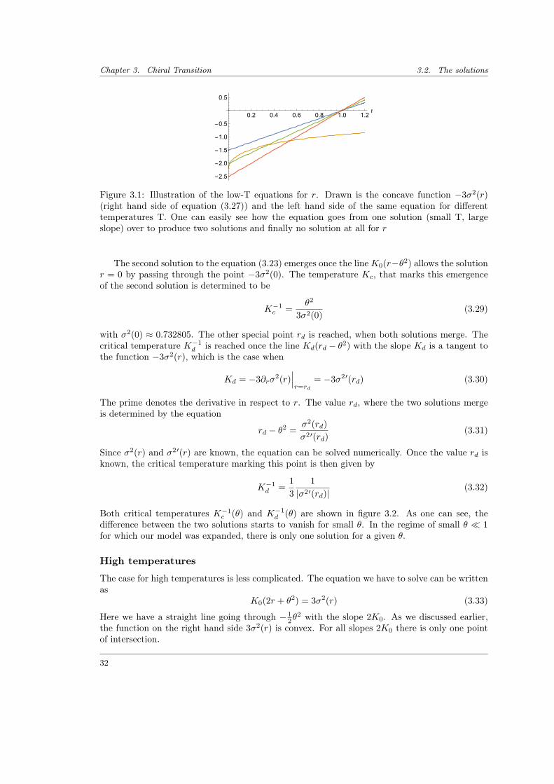
Chapter 3. Chiral Transition 3.2. The solutions

0.2 0.4 0.6 0.8 1.0 1.2r

-2.5

-2.0

-1.5

-1.0

-0.5

0.5

Figure 3.1: Illustration of the low-T equations for r. Drawn is the concave function −3σ2(r)(right hand side of equation (3.27)) and the left hand side of the same equation for differenttemperatures T. One can easily see how the equation goes from one solution (small T, largeslope) over to produce two solutions and finally no solution at all for r

The second solution to the equation (3.23) emerges once the lineK0(r−θ2) allows the solutionr = 0 by passing through the point −3σ2(0). The temperature Kc, that marks this emergenceof the second solution is determined to be

K−1c =

θ2

3σ2(0)(3.29)

with σ2(0) ≈ 0.732805. The other special point rd is reached, when both solutions merge. Thecritical temperature K−1

d is reached once the line Kd(rd − θ2) with the slope Kd is a tangent tothe function −3σ2(r), which is the case when

Kd = −3∂rσ2(r)

∣∣∣r=rd

= −3σ2′(rd) (3.30)

The prime denotes the derivative in respect to r. The value rd, where the two solutions mergeis determined by the equation

rd − θ2 =σ2(rd)

σ2′(rd)(3.31)

Since σ2(r) and σ2′(r) are known, the equation can be solved numerically. Once the value rd isknown, the critical temperature marking this point is then given by

K−1d =

1

3

1

|σ2′(rd)|(3.32)

Both critical temperatures K−1c (θ) and K−1

d (θ) are shown in figure 3.2. As one can see, thedifference between the two solutions starts to vanish for small θ. In the regime of small θ 1for which our model was expanded, there is only one solution for a given θ.

High temperatures

The case for high temperatures is less complicated. The equation we have to solve can be writtenas

K0(2r + θ2) = 3σ2(r) (3.33)

Here we have a straight line going through − 12θ

2 with the slope 2K0. As we discussed earlier,the function on the right hand side 3σ2(r) is convex. For all slopes 2K0 there is only one pointof intersection.

32

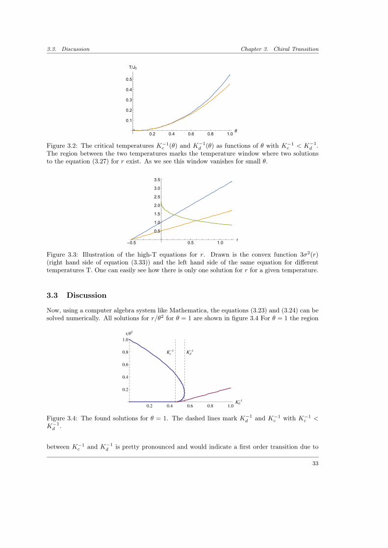
3.3. Discussion Chapter 3. Chiral Transition

0.2 0.4 0.6 0.8 1.0θ

0.1

0.2

0.3

0.4

0.5

T/J0

Figure 3.2: The critical temperatures K−1c (θ) and K−1

d (θ) as functions of θ with K−1c < K−1

d .The region between the two temperatures marks the temperature window where two solutionsto the equation (3.27) for r exist. As we see this window vanishes for small θ.

-0.5 0.5 1.0r

0.5

1.0

1.5

2.0

2.5

3.0

3.5

Figure 3.3: Illustration of the high-T equations for r. Drawn is the convex function 3σ2(r)(right hand side of equation (3.33)) and the left hand side of the same equation for differenttemperatures T. One can easily see how there is only one solution for r for a given temperature.

3.3 Discussion

Now, using a computer algebra system like Mathematica, the equations (3.23) and (3.24) can besolved numerically. All solutions for r/θ2 for θ = 1 are shown in figure 3.4 For θ = 1 the region

0.2 0.4 0.6 0.8 1.0K0

-1

0.2

0.4

0.6

0.8

1.0

rΘ2

Kc-1 Kd

-1

Figure 3.4: The found solutions for θ = 1. The dashed lines mark K−1d and K−1

c with K−1c <

K−1d .

between K−1c and K−1

d is pretty pronounced and would indicate a first order transition due to

33

Chapter 3. Chiral Transition 3.3. Discussion

the jump in order parameter. As we discussed earlier, this window decreases rapidly for small θ,approaching a continuous change in the order parameter. The variational approach is known towrongly capture a second order transition as a first order one.

A prominent example is the variational study of the XY model discussed by Patashinskii andPokrovskii in [53]. Here the continuous phase transition, will lead to a jump in the fitted orderparameter. Without further knowledge this would cause one to believe the transition to be firstorder, which is clearly wrong. In a similar model, the same effect has been discussed by Pytte,[54]. The transition is believed to be continuous and the jump in order parameter is an artifactof the variational method.

The chiral transition is indicated by a vanishing r = 0. For the critical temperature K−1c of

the chiral transition we then simply find

K−1c =

θ2

3σ2(0)∝ θ2 (3.34)

34

4. Renormalization Group

In the previous chapter we focused on the chiral transition using a variational approach. Herethe compact nature of the angles φ(x) was ignored and in extension vortices. Now we will focuson the vortices in the system and their influence on the magnetic phase transition in order toobtain a complete picture. As we saw when discussing the model in section 2.1, the system isdescribed by

βH =K0

2

∫d2x

[1

4(φ2x − θ2)2 + φ2

y +1

4φ2xx

]. (4.1)

To shorten the equations, we have introduced the short hand notation for the derivatives asφx ≡ ∂xφ. Each subscript marks one derivative, so φxx is the second derivative of φ in respectto x. Without the constant energy offset 1

2θ4, the model is simply

βH =K0

2

∫d2x

[−1

2θ2φ2

x + φ2y +

1

4φ2xx +

1

4φ4x

](4.2)

and can be substituted by the effective model

βH =K0

2

∫x

[rφ2

x + φ2y +

1

4φ2xx +

u

4N [φ4

x]

](4.3)

with the parameters r and u. Here N [φ4x] = φ4

x−6σ2φ2x+σ4 is the normal ordering and σ2 = 〈φ2

x〉is the same fluctuation term as used in the previous chapter, [40]. In this model,

ξx =1√r

ξy =1

r(4.4)

can be directly identified as playing the role of the correlation length in x- and y-direction.

4.1 Vortices

Now, in order to focus on vortices, let us consider a region of the dimensions Lx and Ly. We canrescale the system with x/Lx 7→ x and y/Ly 7→ y and introduce the parameters λα = ξα/Lα.The linearized saddle point equation for the system after this rescaling is

λ2xφxx −

1

4λ4xφxxxx + λ2

yφyy = 0 (4.5)

[40]. Analogous to the classical XY model, the angle φ can be split into a spin-wave part φs andvortex part φv. Both do not interact. The spin wave part φs, which carries the chiral order, willbe treated using the RG method later in this chapter.

The saddle-point equation (4.5) with an additional inhomogeneous part δ(x) on the right-hand side describes a vortex. This equation cannot be solved analytically. On small scales, largemomenta, the φxx can be ignored compared to the φxxxx term. This is equivalent to settingr = 0. In this case the scaling between length in y-direction and x-direction is easily identified

35

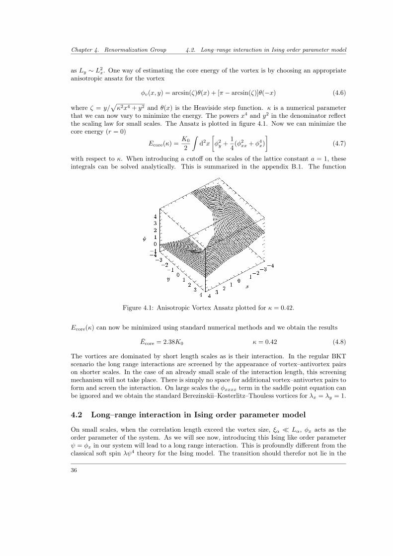
Chapter 4. Renormalization Group 4.2. Long–range interaction in Ising order parameter model

as Ly ∼ L2x. One way of estimating the core energy of the vortex is by choosing an appropriate

anisotropic ansatz for the vortex

φv(x, y) = arcsin(ζ)θ(x) + [π − arcsin(ζ)]θ(−x) (4.6)

where ζ = y/√κ2x4 + y2 and θ(x) is the Heaviside step function. κ is a numerical parameter

that we can now vary to minimize the energy. The powers x4 and y2 in the denominator reflectthe scaling law for small scales. The Ansatz is plotted in figure 4.1. Now we can minimize thecore energy (r = 0)

Ecore(κ) =K0

2

∫d2x

[φ2y +

1

4(φ2xx + φ4

x)

](4.7)

with respect to κ. When introducing a cutoff on the scales of the lattice constant a = 1, theseintegrals can be solved analytically. This is summarized in the appendix B.1. The function

Figure 4.1: Anisotropic Vortex Ansatz plotted for κ = 0.42.

Ecore(κ) can now be minimized using standard numerical methods and we obtain the results

Ecore = 2.38K0 κ = 0.42 (4.8)

The vortices are dominated by short length scales as is their interaction. In the regular BKTscenario the long range interactions are screened by the appearance of vortex–antivortex pairson shorter scales. In the case of an already small scale of the interaction length, this screeningmechanism will not take place. There is simply no space for additional vortex–antivortex pairs toform and screen the interaction. On large scales the φxxxx term in the saddle point equation canbe ignored and we obtain the standard Berezinskii–Kosterlitz–Thouless vortices for λx = λy = 1.

4.2 Long–range interaction in Ising order parameter model

On small scales, when the correlation length exceed the vortex size, ξα Lα, φx acts as theorder parameter of the system. As we will see now, introducing this Ising like order parameterψ = φx in our system will lead to a long range interaction. This is profoundly different from theclassical soft spin λψ4 theory for the Ising model. The transition should therefor not lie in the

36

4.3. RG - small scales Chapter 4. Renormalization Group

Onsager universality class. Later, after doing more rigorous calculations, we will indeed see thatthe critical exponents are different from the Onsager ones.

Starting with the effective Hamiltonian H, equation (4.3), we switch to the order parameterψ ≡ φx. The only non-trivial part of the Hamiltonian will be due to the φ2

y-proportional term

Hy =K0

2

∫d2xφ2

y (4.9)

Using the Fourier transform, as e.g. discussed in [5]

f(x) =1

Ld

∑k

eıkxfk fk =

∫ddx e−ıkxf(x) (4.10)

this interaction transforms to

Hy =K0

2

∑k

k2y|φk|2 =

K0

2

∑k

k2y

k2x

|ψk|2 (4.11)

In the last step we already switched to our new order parameter ψ by using ψk ≡ ıkxφk. Nowwe want to transform this expression back into position space. The back transformation of thek2y part is simple and returns the partial derivatives ∂y in y. The complicated and therefor

interesting term revolves around the back transformation of the 1/k2x interaction.

A =

∫dkx2π

eıkxx

k2x

= −1

2|x| (4.12)

The Fourier transform can be solve by a computer algebra system, e.g. Mathematica. Anotherapproach is to realize that the second derivative of this function is ∂2

xA = −δ(x). In this casethe integral can be written as A = −1/2(xθ(x)− xθ(−x)) with

∂2xA = −∂x

[1

2(θ(x)− θ(−x) + 2xδ(x))

]= −δ(x) (4.13)

Combining the result with the y-back transform, we have the following long range interaction inposition space.

−1

2

∫d2x

∫dx′ψy(x, y)|x− x′|ψy(x′, y) (4.14)

4.3 RG - small scales

The consideration of different length scales that we did for the vortices, is also important whendoing the renormalization group approach. We will be starting with small scales, where thecorrelation length ξ exceeds the system size in each direction. Following the standard approachfrom [5], we can write down the RG flow equations for the parameters r, K, u and the vortexfugacity y. The initial values for these parameters are given by r0 1, u0 = 1, K0 andy0 = exp(−Ecore), with the vortex core energy as we have estimated earlier. As will discussed inmore detail later, when focusing on the anomalous scaling dimension of the system, the u termis not marginal in d = 2. The critical dimension of the system is dc = 5/2. We will extend they-dimension into a (d−1)-dimensional vector and perform the flow calculations as perturbationsin the small parameter ε = 5/2− d. The RG procedure starts by integrating out the fluctuationin φk limited by the momentum shell

π2 >1

4k4x + k2

y > π2e−2l (4.15)

37

Chapter 4. Renormalization Group 4.4. RG - large scales

with the small scale parameter l, and finally rescaling the parameters according to

x = x′el/2 y = y′el r′ = rel (4.16)

We do not rescale φ as it is a compact variable and we want to treat it as such. u is not rescaledas well. The flow equations that we obtain as a result are

d lnu

dl= − 9

2π3

u

K

d ln r

dl= 1− 9

6π3

u

K(4.17)

We discussed earlier, that on the small scales there is no screening due to vortices. Consequentlythe vortex fugacity y = exp(−K) and K only change via rescaling, meaning

dK

dl= −ε d ln y

dl=

3

2(4.18)

The rescaling of the vortex fugacity y = exp(−Ecore +S) is due to the entropy S, correspondingto the change in area

S = ln

(xy

x′y′

)=

3

2l (4.19)

The RG procedure stops when we reach rlc ≈ 1 with elc ≡ ξy. Integrating the flow equations(4.17) produces

ξy =2

tθ2P (4.20)

t =K0

K− 1 (4.21)

P(ξy) = 1 +9

2π3

1

εK0(ξεy − 1) (4.22)

The critical region of the chiral transition marked by9

2π3

1

εK0ξεy 1 (4.23)

we find for the correlation length ξy and the correlation length exponent νy

ξy ∼1

θ2|t|−νy ν−1

y = 1− ε

3(4.24)

From the general scaling for the correlation lengths we see ν−1y = (2νx)−1. Systems with an

anistoropic Lifshitz point, such as the one discussed here, were also studied by Hornreich etal. using a Ginzburg–Landau expansion, [55]. They found the anisotropic scaling law

νx(d− 1)νy = 2− α (4.25)

which is satisfied for α = νyε/3.

4.4 RG - large scales

On large scales l > lc the non-linear terms of our system can be ignored. In this case, the vorticesare just the standard BKT vortices and for d = 2 the flow equations are just the standard BKTequations

d

dlK−1 = 4π3y2 dy

dl= (2− πK)y (4.26)

as can be found in [5]. Unlike the flow equations for the small scales, these equations cannot beeasily integrated.

38

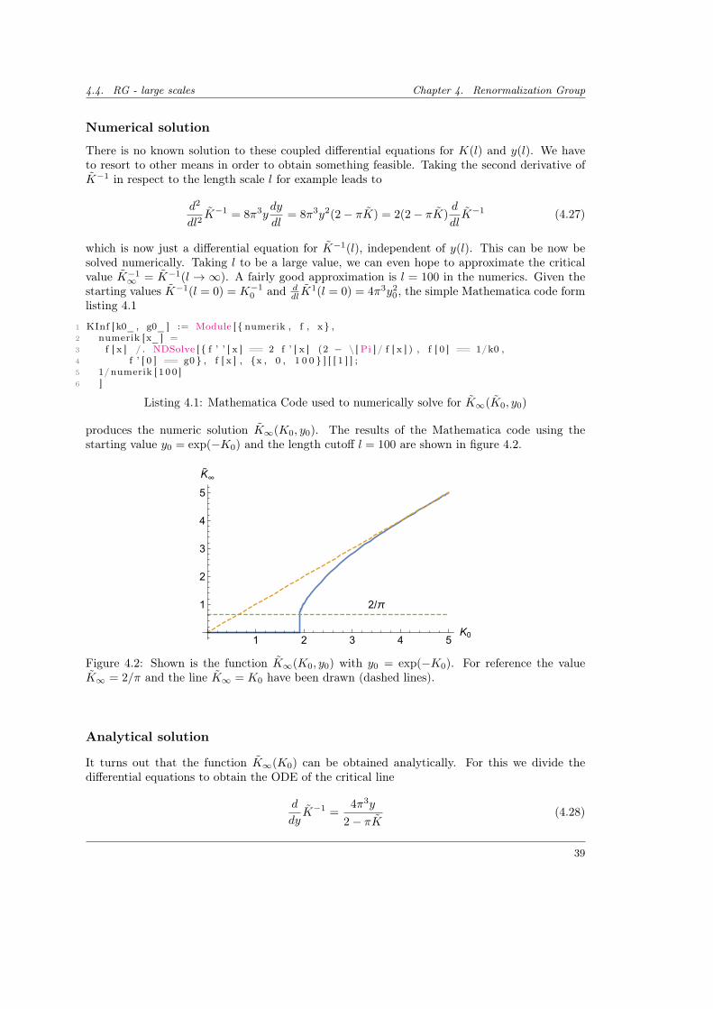
4.4. RG - large scales Chapter 4. Renormalization Group

Numerical solution

There is no known solution to these coupled differential equations for K(l) and y(l). We haveto resort to other means in order to obtain something feasible. Taking the second derivative ofK−1 in respect to the length scale l for example leads to

d2

dl2K−1 = 8π3y

dy

dl= 8π3y2(2− πK) = 2(2− πK)

d

dlK−1 (4.27)

which is now just a differential equation for K−1(l), independent of y(l). This can be now besolved numerically. Taking l to be a large value, we can even hope to approximate the criticalvalue K−1

∞ = K−1(l → ∞). A fairly good approximation is l = 100 in the numerics. Given thestarting values K−1(l = 0) = K−1

0 and ddlK

1(l = 0) = 4π3y20 , the simple Mathematica code form

listing 4.1

1 KInf [ k0_ , g0_ ] := Module [ numerik , f , x ,2 numerik [x_] =3 f [ x ] / . NDSolve [ f ’ ’ [ x ] == 2 f ’ [ x ] (2 − \ [ Pi ] / f [ x ] ) , f [ 0 ] == 1/k0 ,4 f ’ [ 0 ] == g0 , f [ x ] , x , 0 , 1 0 0 ] [ [ 1 ] ] ;5 1/numerik [ 1 0 0 ]6 ]

Listing 4.1: Mathematica Code used to numerically solve for K∞(K0, y0)

produces the numeric solution K∞(K0, y0). The results of the Mathematica code using thestarting value y0 = exp(−K0) and the length cutoff l = 100 are shown in figure 4.2.

1 2 3 4 5K0

1

2

3

4

5

K˜∞

2/π

Figure 4.2: Shown is the function K∞(K0, y0) with y0 = exp(−K0). For reference the valueK∞ = 2/π and the line K∞ = K0 have been drawn (dashed lines).

Analytical solution

It turns out that the function K∞(K0) can be obtained analytically. For this we divide thedifferential equations to obtain the ODE of the critical line

d

dyK−1 =

4π3y

2− πK(4.28)

39

Chapter 4. Renormalization Group 4.4. RG - large scales

This equation is separable

dK−1

(2− π

K−1

)= dy(4π3y) (4.29)

and we can integrate both sides, using the starting values K−10 and y0.

2

(1

K− 1

K0

)− π ln

(K0

K

)= 2π3(y2 − y2

0) (4.30)

Taking the exp(. . . ) on both sides leaves us with

K

K0exp(

2

π(K−1 −K−1

0 )) = exp(2π2(y2 − y20)) (4.31)

This equation can be solved for K, where the solution is related to the Lambert W function. Tomake this connection more clear, we will introduce the constants c1 and c2 to contain everythingbut the K dependency leading to

K exp

(c1

K

)= c2 (4.32)

c1 = 2/π (4.33)

c2 = K0 exp

(2π2(y2 − y2

0) +2

π

1

K0

)(4.34)

The Lambert W function is defined as the inverse to xex = y, so the function W (y) satisfies theidentity

W (y) exp(W (y)) = y (4.35)

The defining equation for W (y) looks very similar to our equation (4.32). Indeed we can use theknowledge of W (y) 1 to solve for K(y) as

K(y) = − c1W (−c1/c2)

(4.36)

K−1(y) = − 1

c1W (−c1/c2) (4.37)

Combined with y0 = exp(−K0) this leads to the expressions

K∞(K0) = − 2

πW(− 2πK0

exp(

2π2e−2K0 − 2πK0

)) (4.38)

K−1∞ (K0) = −π

2W

(− 2

πK0exp

(2π2e−2K0 − 2

πK0

))(4.39)

We can now compare this analytic solution to the one obtained earlier by numerically integratingthe equations for K. The results are pictured in figure 4.3 and show excellent agreement. Theequation for K(y) can also be inverted to

y = ± 1√2π

√√√√ln

(c0e2K−1/π

K−1

)(4.40)

c0 = K0 exp

(2

πK0− 2π2y2

0

)(4.41)

1The Lambert W function is referred to as ProductLog in Mathematica

40

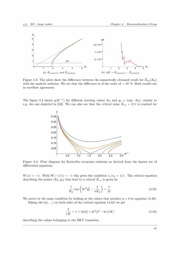
4.4. RG - large scales Chapter 4. Renormalization Group

1 2 3 4 5K0

1

2

3

4

5

K˜∞

2/π

(a) Knumerics and Kanalytic

1 2 3 4 5K0

5.×10-9

1.×10-8

1.5×10-8

ΔK˜

(b) ∆K = Knumerics − Kanalytic

Figure 4.3: The plots show the difference between the numerically obtained result for K∞(K0)with the analytic solution. We see that the difference is of the order of ∼ 10−9. Both results arein excellent agreement.

The figure 4.4 shows y(K−1) for different starting values K0 and y0 = exp(−K0), similar toe.g. the one depicted in [10]. We can also see that the critical value K∞ = 2/π is reached for

0.5 1.0 1.5 2.0 2.5 3.0K-1

0.05

0.10

0.15

0.20

0.25

0.30

0.35

y

Figure 4.4: Flow diagram for Kosterlitz recursion relations as derived from the known set ofdifferential equations.

W (x) = −1. With W (−1/e) = −1 this gives the condition c1/c2 = 1/e. The critical equationdescribing the points (K0, y0) that lead to a critical K∞ is given by

1

K0exp

(2π2y2

0 −2

πK0

)=

π

2e(4.42)

We arrive at the same condition by looking at the values that produce y = 0 in equation (4.40).Taking the ln(. . . ) on both sides of the critical equation (4.42) we get

2

πK= 1 + ln(2) + 2π2y2 − ln (πK) (4.43)

describing the values belonging to the BKT transition.

41

Chapter 4. Renormalization Group 4.5. Anomalous dimension of chiral transition

4.5 Anomalous dimension of chiral transition

Now let us focus specifically on the anomalous scaling dimension of the chiral system.

βH =

∫dx

∫dd−1y

[1

2rφ2

x +1

2φ2y +

1

8φ2xx + uφ4

x

](4.44)

where we extended d → 5/2 to make the interaction term uφ4x marginal and enable a RG

calculation. Using the following rescaling

x 7→ x′ = x/b r 7→ r′ = b∆rr φ 7→ φ′ = b∆φφ

y 7→ y′ = y/bz u 7→ u′ = b∆uu

Fixing the scaling of the two gradient terms φ2y and φ2

xx fixes the dynamical exponent z = 2,leaving the integral to scale as∫

dxdd−1y 7→ b1+2(d−1)

∫dx′ dd−1y′ (4.45)

With the condition that the gradients should not scale with b, we get ∆φ = d− 5/2. The otherscaling exponents follow leaving us with

∆r = 2 ∆φ = d− 5

2= −ε ∆u = 5− 2d = 2ε z = 2

Now we will consider the perturbation around the dimension dc = 5/2 in the small parameterε = 5/2− d.

Fix point u∗ to first order in ε

In order to compute the first order correction to the scaling in u we have to write down the firstloop corrections due to

= −36u2

∫ Λ

Λ/b

dkx2π

d3/2k⊥(2π)3/2

k4x

(k2⊥ + 1

4k4x)2

= −36u2 K3/2

(2π)5/2ln(b) (4.46)

where the combinatorial pre-factor consists of 12 ∗

(42

)∗ 2 ∗

(42

)= 36 and the vertices giv-

ing a (−1)(−u)2 contribution. We used the general change to spherical coordinates∫

ddx =Kd

∫dr rd−1 with Kd = 2πd/2/Γ(d/2). This leads to the one-loop rescaling of u as

u′ = b2ε[u− 36u2 K3/2

(2π)5/2ln(b)

]⇒ u∗ =

(2π)5/2

36K3/2

(1− b2ε)ln(b)

≈ (2π)5/2

18K3/2ε+O(ε2) (4.47)

with the non-trivial fix point u∗.

2-loop correction to the self energy

Looking at the scaling relations, the full propagator G = 〈∂xφ∂xφ〉 ∝ x−2−2∆φ ∝ k2−2∆φx with

∆φ = ∆φ + ∆(ε)φ . With d = 5/2 as we saw before, ∆φ = 0 and the full propagator scaling can be

42

4.5. Anomalous dimension of chiral transition Chapter 4. Renormalization Group

expanded in ∆(ε)φ

G ∝ k2x

[1− 2∆

(ε)φ ln(kx) + . . .

](4.48)

G−1 = G−1 − Σ =k2⊥k2x

+1

4k2x − Σ(0)− (Σ(k)− Σ(0)) (4.49)

So the change in k2x due to the self energy correction ∆Σ = Σ(k)−Σ(0) determines the anomalous

dimension ∆(ε)φ logarithmic in scale ln(b) leading to

∆(ε)φ =

2

k2x

∂∆Σ

∂ ln(b)(4.50)

The first rescaling of the k dependency of the self energy Σ is given by the two loop diagram

∆Σ = Σ(k)− Σ(0) =

= −48u∗2

∫dx

∫d3/2y G3(x,y)

(eıkxx+ık⊥y − 1

)(4.51)

with the combinatorial pre-factor for the diagram being 12 ∗(

41

)∗ 3! ∗

(41

)= 48 and the vertices

give an additional (−1)(−u)2. Here we work with the propagator in position space, removingthe hassle of having to integrate over all internal momenta of the diagram. This technique isdiscussed in detail by Patashinskii and Pokrovskii in [53]. With k⊥ = 0 the first correction to k2

x

can be calculated by expanding the integrand in order of kx (neglecting k⊥ terms) finding thecorrection to be

∆Σ ≈ k2x

[24u∗2

∫ ∞−∞

dx

∫ ∞−∞

d3/2y x2G3(x,y)

]Here the correlator of the ∂xφ fields is given as

G(x,y) =

∫dkx2π

d3/2k⊥(2π)3/2

k2x

k2⊥ + 1

4k4x

eıkxxeık⊥y =1

yf

(x2

y

)(4.52)

Amazingly, this Fourier transform can be done exactly. A detailed calculation is done in theappendix B.5. It also includes a second approach where the problem is reduced to a differentialequation which can also be solved exactly, producing the same result.

f(z) =z3/4

4π14

(I− 3

4

(z2

)−LLL− 3

4

(z2

))where Iν is the modified Bessel function of the first kind and LLLν the modified Struve function.The corrections in k2

x can then be written as

∆Σ = k2x

[24u∗2K3/2

∫ ∞−∞

dx

∫ ∞0

dyx2

y5/2f3

(x2

y

)]= k2

x

[24u∗2K3/2

∫ ∞0

dy

y

∫ ∞0

dz√zf3(z)︸ ︷︷ ︸

≡cx

]

= k2x

[24u∗2K3/2cx ln(b)

](4.53)

43

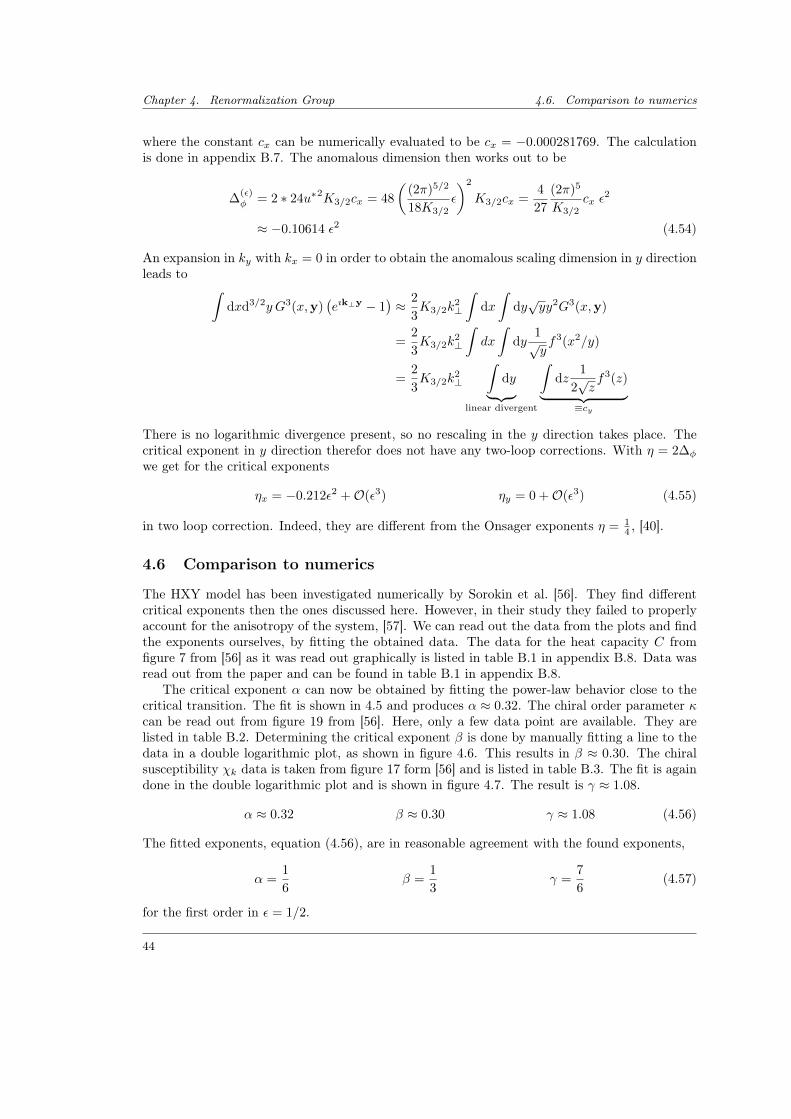
Chapter 4. Renormalization Group 4.6. Comparison to numerics

where the constant cx can be numerically evaluated to be cx = −0.000281769. The calculationis done in appendix B.7. The anomalous dimension then works out to be

∆(ε)φ = 2 ∗ 24u∗2K3/2cx = 48

((2π)5/2

18K3/2ε

)2

K3/2cx =4

27

(2π)5

K3/2cx ε

2

≈ −0.10614 ε2 (4.54)

An expansion in ky with kx = 0 in order to obtain the anomalous scaling dimension in y directionleads to ∫

dxd3/2y G3(x,y)(eık⊥y − 1

)≈ 2

3K3/2k

2⊥

∫dx

∫dy√yy2G3(x,y)

=2

3K3/2k

2⊥

∫dx

∫dy

1√yf3(x2/y)

=2

3K3/2k

2⊥

∫dy︸ ︷︷ ︸

linear divergent

∫dz

1

2√zf3(z)︸ ︷︷ ︸

≡cy

There is no logarithmic divergence present, so no rescaling in the y direction takes place. Thecritical exponent in y direction therefor does not have any two-loop corrections. With η = 2∆φ

we get for the critical exponents

ηx = −0.212ε2 +O(ε3) ηy = 0 +O(ε3) (4.55)

in two loop correction. Indeed, they are different from the Onsager exponents η = 14 , [40].

4.6 Comparison to numerics

The HXY model has been investigated numerically by Sorokin et al. [56]. They find differentcritical exponents then the ones discussed here. However, in their study they failed to properlyaccount for the anisotropy of the system, [57]. We can read out the data from the plots and findthe exponents ourselves, by fitting the obtained data. The data for the heat capacity C fromfigure 7 from [56] as it was read out graphically is listed in table B.1 in appendix B.8. Data wasread out from the paper and can be found in table B.1 in appendix B.8.

The critical exponent α can now be obtained by fitting the power-law behavior close to thecritical transition. The fit is shown in 4.5 and produces α ≈ 0.32. The chiral order parameter κcan be read out from figure 19 from [56]. Here, only a few data point are available. They arelisted in table B.2. Determining the critical exponent β is done by manually fitting a line to thedata in a double logarithmic plot, as shown in figure 4.6. This results in β ≈ 0.30. The chiralsusceptibility χk data is taken from figure 17 form [56] and is listed in table B.3. The fit is againdone in the double logarithmic plot and is shown in figure 4.7. The result is γ ≈ 1.08.

α ≈ 0.32 β ≈ 0.30 γ ≈ 1.08 (4.56)

The fitted exponents, equation (4.56), are in reasonable agreement with the found exponents,

α =1

6β =

1

3γ =

7

6(4.57)

for the first order in ε = 1/2.

44

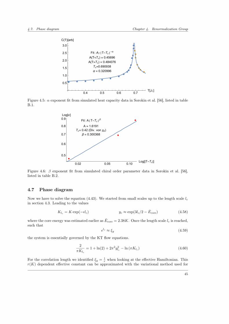
4.7. Phase diagram Chapter 4. Renormalization Group

0.4 0.5 0.6 0.7T[J1]

0.5

1.0

1.5

2.0

2.5

3.0

C(T)[arb]

Fit : ATT-Tc-α

A(T<Tc) = 0.45696

A(T>Tc) = 0.484076

Tc=0.690938

α = 0.320996

Figure 4.5: α exponent fit from simulated heat capacity data in Sorokin et al. [56], listed in tableB.1.

0.02 0.05 0.10Log[|T-Tc|]

0.5

0.6

0.7

0.8

0.9Log[κ]

Fit : AT-Tcβ

A = 1.6191Tc= 0.42 (Div. von χk)

β = 0.300368

Figure 4.6: β exponent fit from simulated chiral order parameter data in Sorokin et al. [56],listed in table B.2.

4.7 Phase diagram

Now we have to solve the equation (4.43). We started from small scales up to the length scale lcin section 4.3. Leading to the values

Klc = K exp(−εlc) yc ≈ exp(3lc/2− Ecore) (4.58)

where the core energy was estimated earlier as Ecore = 2.38K. Once the length scale lc is reached,such that

elc ≈ ξy (4.59)

the system is essentially governed by the KT flow equations.

2

πKlc

= 1 + ln(2) + 2π2y2lc − ln (πKlc) (4.60)

For the correlation length we identified ξy = 1r when looking at the effective Hamiltonian. This

r(K) dependent effective constant can be approximated with the variational method used for

45

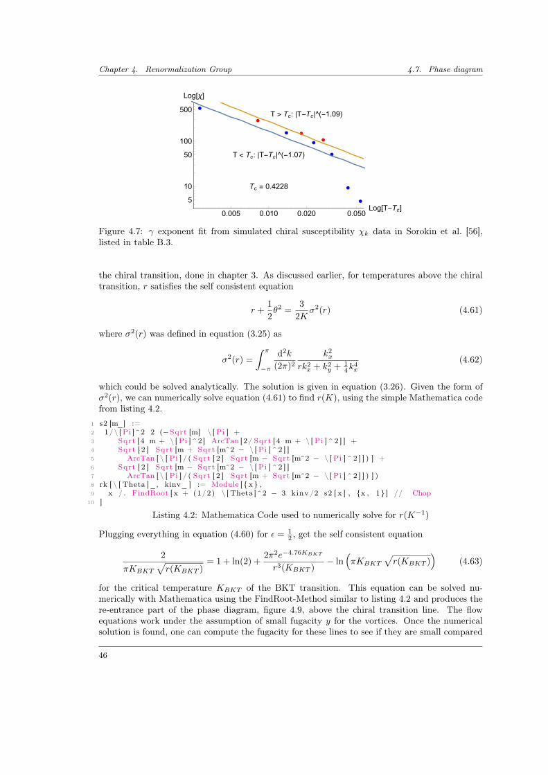
Chapter 4. Renormalization Group 4.7. Phase diagram

0.005 0.010 0.020 0.050Log[T-Tc]

5

10

50

100

500

Log[χ]

T > Tc: |T-Tc|^(-1.09)

T < Tc: |T-Tc|^(-1.07)

Tc = 0.4228

Figure 4.7: γ exponent fit from simulated chiral susceptibility χk data in Sorokin et al. [56],listed in table B.3.

the chiral transition, done in chapter 3. As discussed earlier, for temperatures above the chiraltransition, r satisfies the self consistent equation

r +1

2θ2 =

3

2Kσ2(r) (4.61)

where σ2(r) was defined in equation (3.25) as

σ2(r) =

∫ π

−π

d2k

(2π)2

k2x

rk2x + k2

y + 14k

4x

(4.62)

which could be solved analytically. The solution is given in equation (3.26). Given the form ofσ2(r), we can numerically solve equation (4.61) to find r(K), using the simple Mathematica codefrom listing 4.2.

1 s2 [m_] :=2 1/\ [ Pi ]^2 2 (−Sqrt [m] \ [ Pi ] +3 Sqrt [ 4 m + \ [ Pi ] ^2 ] ArcTan [2/ Sqrt [ 4 m + \ [ Pi ] ^ 2 ] ] +4 Sqrt [ 2 ] Sqrt [m + Sqrt [m^2 − \ [ Pi ] ^ 2 ] ]5 ArcTan [ \ [ Pi ] / ( Sqrt [ 2 ] Sqrt [m − Sqrt [m^2 − \ [ Pi ] ^ 2 ] ] ) ] +6 Sqrt [ 2 ] Sqrt [m − Sqrt [m^2 − \ [ Pi ] ^ 2 ] ]7 ArcTan [ \ [ Pi ] / ( Sqrt [ 2 ] Sqrt [m + Sqrt [m^2 − \ [ Pi ] ^ 2 ] ] ) ] )8 rk [ \ [ Theta ]_, kinv_ ] := Module [ x ,9 x / . FindRoot [ x + (1/2) \ [ Theta ]^2 − 3 kinv /2 s2 [ x ] , x , 1 ] // Chop

10 ]

Listing 4.2: Mathematica Code used to numerically solve for r(K−1)

Plugging everything in equation (4.60) for ε = 12 , get the self consistent equation

2

πKBKT

√r(KBKT )

= 1 + ln(2) +2π2e−4.76KBKT

r3(KBKT )− ln

(πKBKT

√r(KBKT )

)(4.63)

for the critical temperature KBKT of the BKT transition. This equation can be solved nu-merically with Mathematica using the FindRoot-Method similar to listing 4.2 and produces there-entrance part of the phase diagram, figure 4.9, above the chiral transition line. The flowequations work under the assumption of small fugacity y for the vortices. Once the numericalsolution is found, one can compute the fugacity for these lines to see if they are small compared

46

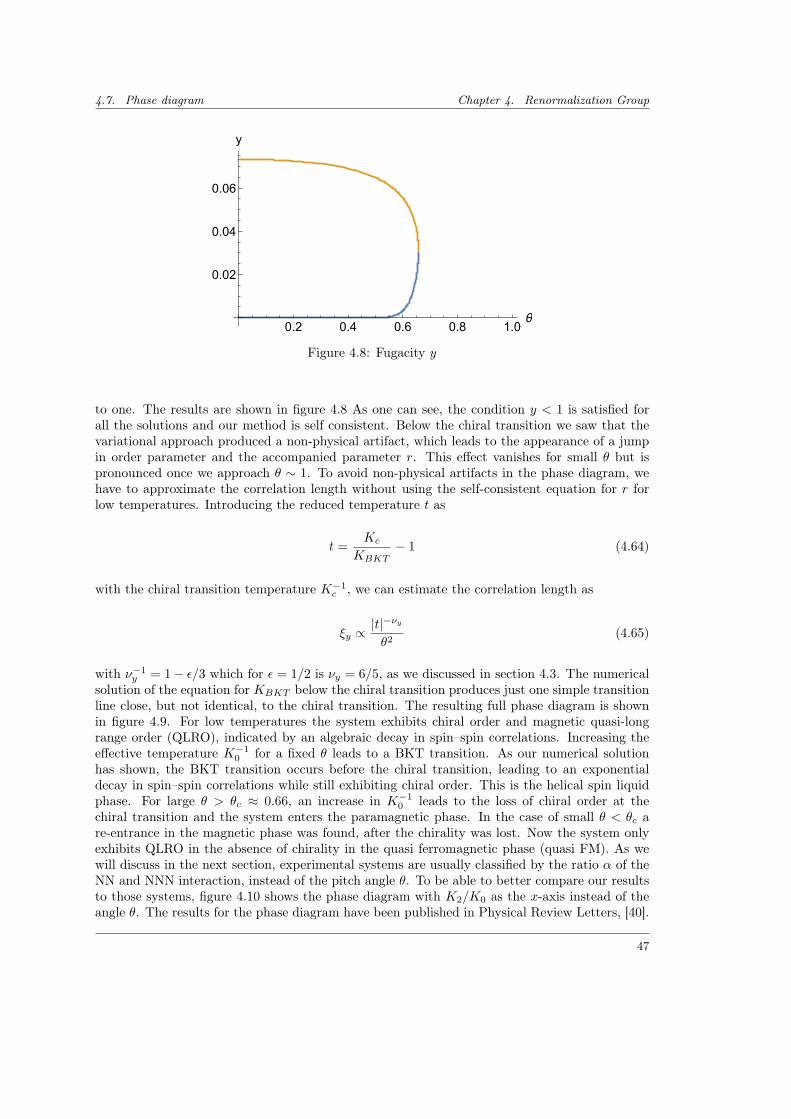
4.7. Phase diagram Chapter 4. Renormalization Group

0.2 0.4 0.6 0.8 1.0θ

0.02

0.04

0.06

y

Figure 4.8: Fugacity y

to one. The results are shown in figure 4.8 As one can see, the condition y < 1 is satisfied forall the solutions and our method is self consistent. Below the chiral transition we saw that thevariational approach produced a non-physical artifact, which leads to the appearance of a jumpin order parameter and the accompanied parameter r. This effect vanishes for small θ but ispronounced once we approach θ ∼ 1. To avoid non-physical artifacts in the phase diagram, wehave to approximate the correlation length without using the self-consistent equation for r forlow temperatures. Introducing the reduced temperature t as

t =Kc

KBKT− 1 (4.64)

with the chiral transition temperature K−1c , we can estimate the correlation length as

ξy ∝|t|−νyθ2

(4.65)

with ν−1y = 1− ε/3 which for ε = 1/2 is νy = 6/5, as we discussed in section 4.3. The numerical

solution of the equation for KBKT below the chiral transition produces just one simple transitionline close, but not identical, to the chiral transition. The resulting full phase diagram is shownin figure 4.9. For low temperatures the system exhibits chiral order and magnetic quasi-longrange order (QLRO), indicated by an algebraic decay in spin–spin correlations. Increasing theeffective temperature K−1

0 for a fixed θ leads to a BKT transition. As our numerical solutionhas shown, the BKT transition occurs before the chiral transition, leading to an exponentialdecay in spin–spin correlations while still exhibiting chiral order. This is the helical spin liquidphase. For large θ > θc ≈ 0.66, an increase in K−1

0 leads to the loss of chiral order at thechiral transition and the system enters the paramagnetic phase. In the case of small θ < θc are-entrance in the magnetic phase was found, after the chirality was lost. Now the system onlyexhibits QLRO in the absence of chirality in the quasi ferromagnetic phase (quasi FM). As wewill discuss in the next section, experimental systems are usually classified by the ratio α of theNN and NNN interaction, instead of the pitch angle θ. To be able to better compare our resultsto those systems, figure 4.10 shows the phase diagram with K2/K0 as the x-axis instead of theangle θ. The results for the phase diagram have been published in Physical Review Letters, [40].

47

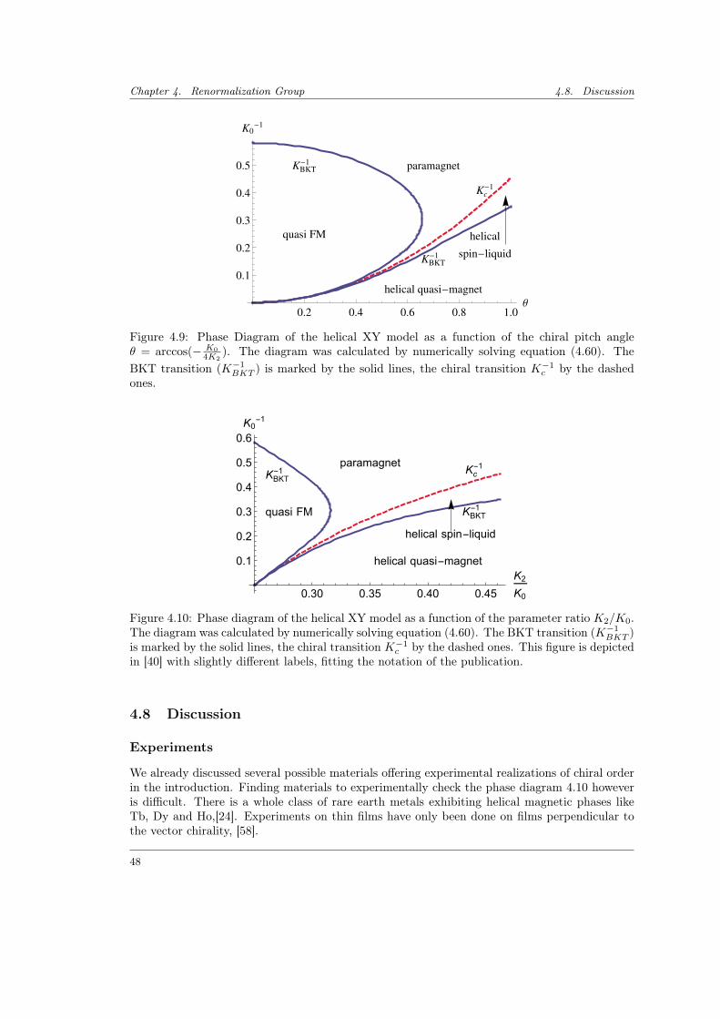
Chapter 4. Renormalization Group 4.8. Discussion

0.2 0.4 0.6 0.8 1.0Θ

0.1

0.2

0.3

0.4

0.5

K0-1

helical quasi-magnet

paramagnet

Kc-1

KBKT-1

helical

spin-liquid

KBKT-1

quasi FM

Figure 4.9: Phase Diagram of the helical XY model as a function of the chiral pitch angleθ = arccos(− K0

4K2). The diagram was calculated by numerically solving equation (4.60). The

BKT transition (K−1BKT ) is marked by the solid lines, the chiral transition K−1

c by the dashedones.

0.30 0.35 0.40 0.45

K2K0

0.1

0.2

0.3

0.4

0.5

0.6K0

-1

helical quasi-magnet

paramagnetKc

-1

KBKT-1

helical spin-liquid

KBKT-1

quasi FM

Figure 4.10: Phase diagram of the helical XY model as a function of the parameter ratio K2/K0.The diagram was calculated by numerically solving equation (4.60). The BKT transition (K−1

BKT )is marked by the solid lines, the chiral transition K−1

c by the dashed ones. This figure is depictedin [40] with slightly different labels, fitting the notation of the publication.

4.8 Discussion

Experiments

We already discussed several possible materials offering experimental realizations of chiral orderin the introduction. Finding materials to experimentally check the phase diagram 4.10 howeveris difficult. There is a whole class of rare earth metals exhibiting helical magnetic phases likeTb, Dy and Ho,[24]. Experiments on thin films have only been done on films perpendicular tothe vector chirality, [58].

48

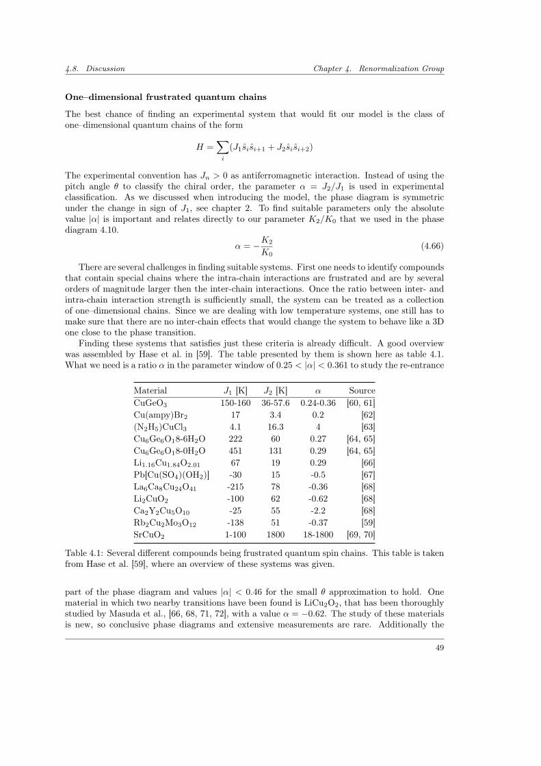
4.8. Discussion Chapter 4. Renormalization Group

One–dimensional frustrated quantum chains

The best chance of finding an experimental system that would fit our model is the class ofone–dimensional quantum chains of the form

H =∑i

(J1sisi+1 + J2sisi+2)

The experimental convention has Jn > 0 as antiferromagnetic interaction. Instead of using thepitch angle θ to classify the chiral order, the parameter α = J2/J1 is used in experimentalclassification. As we discussed when introducing the model, the phase diagram is symmetricunder the change in sign of J1, see chapter 2. To find suitable parameters only the absolutevalue |α| is important and relates directly to our parameter K2/K0 that we used in the phasediagram 4.10.

α = −K2

K0(4.66)

There are several challenges in finding suitable systems. First one needs to identify compoundsthat contain special chains where the intra-chain interactions are frustrated and are by severalorders of magnitude larger then the inter-chain interactions. Once the ratio between inter- andintra-chain interaction strength is sufficiently small, the system can be treated as a collectionof one–dimensional chains. Since we are dealing with low temperature systems, one still has tomake sure that there are no inter-chain effects that would change the system to behave like a 3Done close to the phase transition.

Finding these systems that satisfies just these criteria is already difficult. A good overviewwas assembled by Hase et al. in [59]. The table presented by them is shown here as table 4.1.What we need is a ratio α in the parameter window of 0.25 < |α| < 0.361 to study the re-entrance

Material J1 [K] J2 [K] α SourceCuGeO3 150-160 36-57.6 0.24-0.36 [60, 61]Cu(ampy)Br2 17 3.4 0.2 [62](N2H5)CuCl3 4.1 16.3 4 [63]Cu6Ge6O18-6H2O 222 60 0.27 [64, 65]Cu6Ge6O18-0H2O 451 131 0.29 [64, 65]Li1.16Cu1.84O2.01 67 19 0.29 [66]Pb[Cu(SO4)(OH2)] -30 15 -0.5 [67]La6Ca8Cu24O41 -215 78 -0.36 [68]Li2CuO2 -100 62 -0.62 [68]Ca2Y2Cu5O10 -25 55 -2.2 [68]Rb2Cu2Mo3O12 -138 51 -0.37 [59]SrCuO2 1-100 1800 18-1800 [69, 70]

Table 4.1: Several different compounds being frustrated quantum spin chains. This table is takenfrom Hase et al. [59], where an overview of these systems was given.

part of the phase diagram and values |α| < 0.46 for the small θ approximation to hold. Onematerial in which two nearby transitions have been found is LiCu2O2, that has been thoroughlystudied by Masuda et al., [66, 68, 71, 72], with a value α = −0.62. The study of these materialsis new, so conclusive phase diagrams and extensive measurements are rare. Additionally the

49

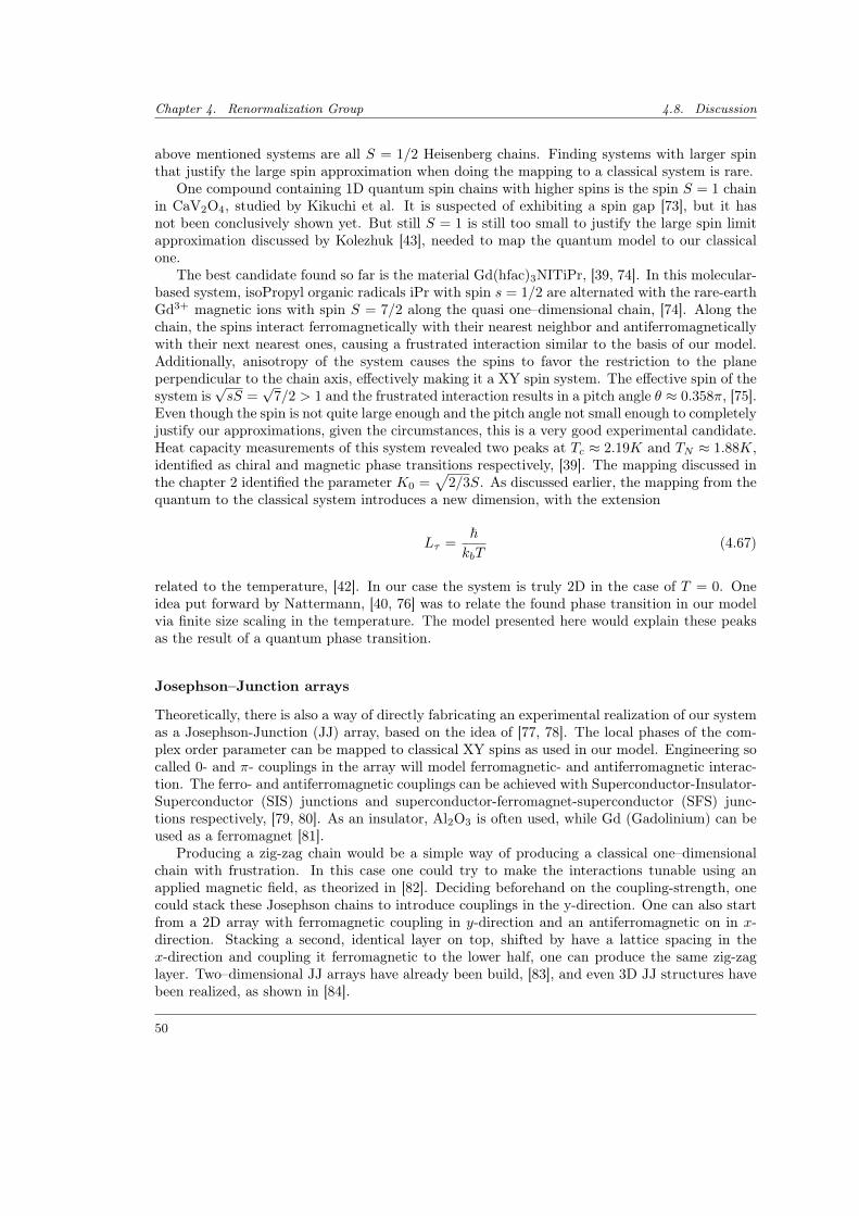
Chapter 4. Renormalization Group 4.8. Discussion

above mentioned systems are all S = 1/2 Heisenberg chains. Finding systems with larger spinthat justify the large spin approximation when doing the mapping to a classical system is rare.

One compound containing 1D quantum spin chains with higher spins is the spin S = 1 chainin CaV2O4, studied by Kikuchi et al. It is suspected of exhibiting a spin gap [73], but it hasnot been conclusively shown yet. But still S = 1 is still too small to justify the large spin limitapproximation discussed by Kolezhuk [43], needed to map the quantum model to our classicalone.

The best candidate found so far is the material Gd(hfac)3NITiPr, [39, 74]. In this molecular-based system, isoPropyl organic radicals iPr with spin s = 1/2 are alternated with the rare-earthGd3+ magnetic ions with spin S = 7/2 along the quasi one–dimensional chain, [74]. Along thechain, the spins interact ferromagnetically with their nearest neighbor and antiferromagneticallywith their next nearest ones, causing a frustrated interaction similar to the basis of our model.Additionally, anisotropy of the system causes the spins to favor the restriction to the planeperpendicular to the chain axis, effectively making it a XY spin system. The effective spin of thesystem is

√sS =

√7/2 > 1 and the frustrated interaction results in a pitch angle θ ≈ 0.358π, [75].

Even though the spin is not quite large enough and the pitch angle not small enough to completelyjustify our approximations, given the circumstances, this is a very good experimental candidate.Heat capacity measurements of this system revealed two peaks at Tc ≈ 2.19K and TN ≈ 1.88K,identified as chiral and magnetic phase transitions respectively, [39]. The mapping discussed inthe chapter 2 identified the parameter K0 =

√2/3S. As discussed earlier, the mapping from the

quantum to the classical system introduces a new dimension, with the extension

Lτ =~kbT

(4.67)

related to the temperature, [42]. In our case the system is truly 2D in the case of T = 0. Oneidea put forward by Nattermann, [40, 76] was to relate the found phase transition in our modelvia finite size scaling in the temperature. The model presented here would explain these peaksas the result of a quantum phase transition.

Josephson–Junction arrays

Theoretically, there is also a way of directly fabricating an experimental realization of our systemas a Josephson-Junction (JJ) array, based on the idea of [77, 78]. The local phases of the com-plex order parameter can be mapped to classical XY spins as used in our model. Engineering socalled 0- and π- couplings in the array will model ferromagnetic- and antiferromagnetic interac-tion. The ferro- and antiferromagnetic couplings can be achieved with Superconductor-Insulator-Superconductor (SIS) junctions and superconductor-ferromagnet-superconductor (SFS) junc-tions respectively, [79, 80]. As an insulator, Al2O3 is often used, while Gd (Gadolinium) can beused as a ferromagnet [81].

Producing a zig-zag chain would be a simple way of producing a classical one–dimensionalchain with frustration. In this case one could try to make the interactions tunable using anapplied magnetic field, as theorized in [82]. Deciding beforehand on the coupling-strength, onecould stack these Josephson chains to introduce couplings in the y-direction. One can also startfrom a 2D array with ferromagnetic coupling in y-direction and an antiferromagnetic on in x-direction. Stacking a second, identical layer on top, shifted by have a lattice spacing in thex-direction and coupling it ferromagnetic to the lower half, one can produce the same zig-zaglayer. Two–dimensional JJ arrays have already been build, [83], and even 3D JJ structures havebeen realized, as shown in [84].

50

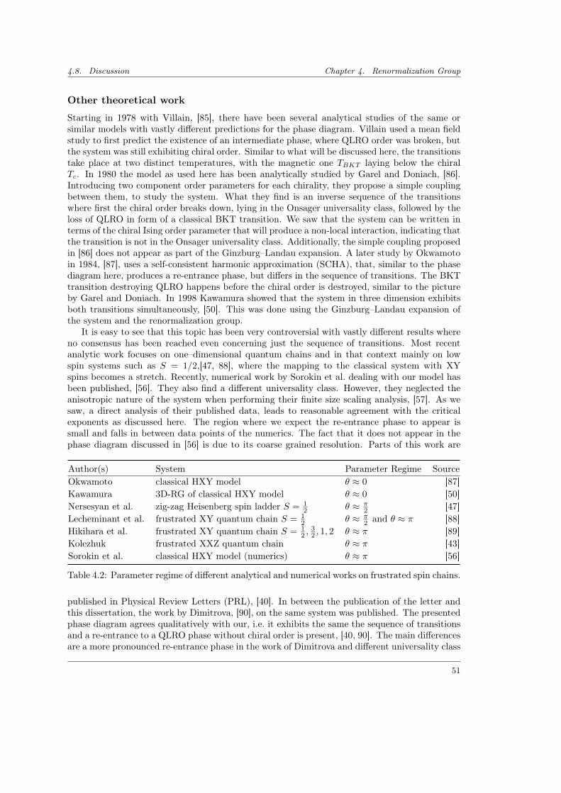
4.8. Discussion Chapter 4. Renormalization Group

Other theoretical work

Starting in 1978 with Villain, [85], there have been several analytical studies of the same orsimilar models with vastly different predictions for the phase diagram. Villain used a mean fieldstudy to first predict the existence of an intermediate phase, where QLRO order was broken, butthe system was still exhibiting chiral order. Similar to what will be discussed here, the transitionstake place at two distinct temperatures, with the magnetic one TBKT laying below the chiralTc. In 1980 the model as used here has been analytically studied by Garel and Doniach, [86].Introducing two component order parameters for each chirality, they propose a simple couplingbetween them, to study the system. What they find is an inverse sequence of the transitionswhere first the chiral order breaks down, lying in the Onsager universality class, followed by theloss of QLRO in form of a classical BKT transition. We saw that the system can be written interms of the chiral Ising order parameter that will produce a non-local interaction, indicating thatthe transition is not in the Onsager universality class. Additionally, the simple coupling proposedin [86] does not appear as part of the Ginzburg–Landau expansion. A later study by Okwamotoin 1984, [87], uses a self-consistent harmonic approximation (SCHA), that, similar to the phasediagram here, produces a re-entrance phase, but differs in the sequence of transitions. The BKTtransition destroying QLRO happens before the chiral order is destroyed, similar to the pictureby Garel and Doniach. In 1998 Kawamura showed that the system in three dimension exhibitsboth transitions simultaneously, [50]. This was done using the Ginzburg–Landau expansion ofthe system and the renormalization group.

It is easy to see that this topic has been very controversial with vastly different results whereno consensus has been reached even concerning just the sequence of transitions. Most recentanalytic work focuses on one–dimensional quantum chains and in that context mainly on lowspin systems such as S = 1/2,[47, 88], where the mapping to the classical system with XYspins becomes a stretch. Recently, numerical work by Sorokin et al. dealing with our model hasbeen published, [56]. They also find a different universality class. However, they neglected theanisotropic nature of the system when performing their finite size scaling analysis, [57]. As wesaw, a direct analysis of their published data, leads to reasonable agreement with the criticalexponents as discussed here. The region where we expect the re-entrance phase to appear issmall and falls in between data points of the numerics. The fact that it does not appear in thephase diagram discussed in [56] is due to its coarse grained resolution. Parts of this work are

Author(s) System Parameter Regime SourceOkwamoto classical HXY model θ ≈ 0 [87]Kawamura 3D-RG of classical HXY model θ ≈ 0 [50]Nersesyan et al. zig-zag Heisenberg spin ladder S = 1

2 θ ≈ π2 [47]

Lecheminant et al. frustrated XY quantum chain S = 12 θ ≈ π

2 and θ ≈ π [88]Hikihara et al. frustrated XY quantum chain S = 1

2 ,32 , 1, 2 θ ≈ π [89]

Kolezhuk frustrated XXZ quantum chain θ ≈ π [43]Sorokin et al. classical HXY model (numerics) θ ≈ π [56]

Table 4.2: Parameter regime of different analytical and numerical works on frustrated spin chains.

published in Physical Review Letters (PRL), [40]. In between the publication of the letter andthis dissertation, the work by Dimitrova, [90], on the same system was published. The presentedphase diagram agrees qualitatively with our, i.e. it exhibits the same the sequence of transitionsand a re-entrance to a QLRO phase without chiral order is present, [40, 90]. The main differencesare a more pronounced re-entrance phase in the work of Dimitrova and different universality class

51

Chapter 4. Renormalization Group 4.8. Discussion

for the chiral transition. As we discussed, we expect that the strong anisotropy of the systemis reflected in the critical exponents, leading to νx 6= νy and ηx 6= ηy in our case. The necessityof replacing each of the simple exponents η and ν by a respective pair in an anisotropic systemwith chiral ground state is also discussed by Hornreich et al., [55]. However the exponents foundby Dimitrova are isotropic, [90]. The procedure used in [90] is based on rewriting the systemas a φ4 theory non-trivially coupled to a free auxiliary field followed by the RG-procedure. Forreasons not quite clear, this is done for dydx2−ε around d = 3 − ε as apposed to an expansionaround the upper critical dimension dc = 4 of the φ4 theory, [90, 91].

52

5. Multiferroics

In this chapter we will take a closer look at the relation between chiral order and polarizationin multiferroic systems. Different mechanisms for the coupling of magnetic and electric orderare discussed and, starting from a symmetry argument, the HXY model will extended by aninteraction with the electric field. The effect of the polarization on the domain walls of thesystem will be studied. The resulting saddle-point equations will be solved perturbatively andare compared to numerical results.

In the previous chapters we discussed the HXY model where a frustrated interaction of theXY spins in x-direction leads to chiral ground state with wave vector ±q = ±(θ/a, 0, 0). Theenergy of the system in terms of the magnetization can be written as

H =J

2a

∫d2x

[−θ

2

2(∂xm)2 +

a2

4(∂2xm)2 + (∂ym)2

](5.1)

similar to [18]. When we are only focusing on the phase fluctuations, as is typical for 2D systems,we obtain

H =J

2a

∫d2x

[−θ

2

2(∂xφ)2 +

a2

4((∂xφ)4 + (∂2

xφ)2) + (∂yφ)2

](5.2)

the same model as derived in chapter 2 equation (2.19) from a microscopic system where ferro-magnetic nearest neighbor interaction competes with an antiferromagnetic next–nearest neighborinteraction, [40]. From this on out we will set the lattice constant a = 1 for convenience. Byshifting the ground state energy by 1

4θ4, we can give the system a form that makes the double

minimum nature of the ∂xφ terms clear

H =J

2

∫d2x

[1

4((∂xφ)2 − θ2)2 + (∂yφ)2 +

1

4(∂2xφ)2

](5.3)

As discussed in the previous chapters and partially published in [40], this model exhibits sequen-tial phases transitions by increasing βJ where first the magnetic order is lost by a BKT transitionfollowed by the loss of chiral order. Additionally a re-entrance to a quasi ferromagnetic statewas found for small angles θ. The phase of interest in the small region of no magnetic orderwhile still exhibiting chiral order is referred to as the helical spin liquid, [40]. The experimen-tal measurement of this phase is complicated when only looking at the magnetic orientation aspointed out by Villain [85], because a 4-point correlator is needed to identify the chiral correla-tions in two different chains in the absence of magnetic ordering. One possible idea to circumventthis complicated measurement is to look at multiferroic materials where the vector chiral orderparameter

κ = 〈Si × Si+1〉 = 〈sin(∂xφ)〉 κ ≈ 〈∂xφ〉 κ (5.4)

can couple to the polarization P of the system. Here the unit vector κ points in the directionperpendicular to the rotation plane of the XY spins Si. In the following sections we will discussmultiferroic materials and the connection of the chiral order and the polarization. With theproper coupling identified we can examine the effect of the polarization on chiral domain walls.We will see that polarization and chiral domains are in one-to-one correspondence.

53

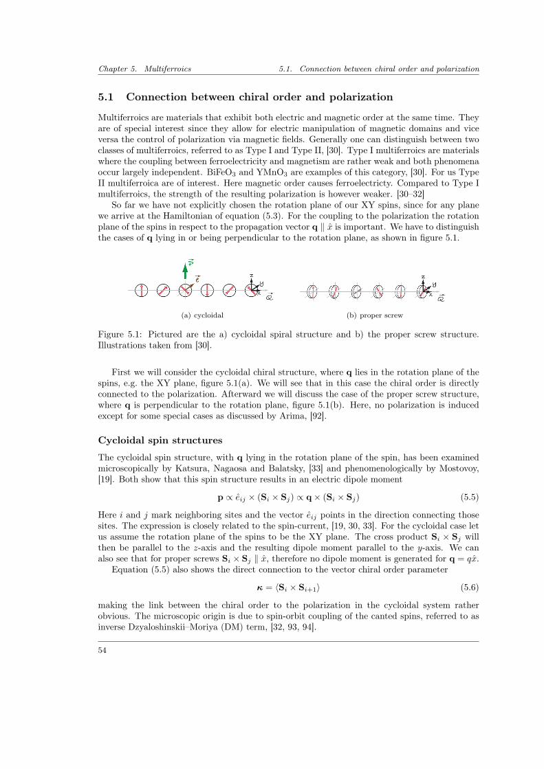
Chapter 5. Multiferroics 5.1. Connection between chiral order and polarization

5.1 Connection between chiral order and polarization

Multiferroics are materials that exhibit both electric and magnetic order at the same time. Theyare of special interest since they allow for electric manipulation of magnetic domains and viceversa the control of polarization via magnetic fields. Generally one can distinguish between twoclasses of multiferroics, referred to as Type I and Type II, [30]. Type I multiferroics are materialswhere the coupling between ferroelectricity and magnetism are rather weak and both phenomenaoccur largely independent. BiFeO3 and YMnO3 are examples of this category, [30]. For us TypeII multiferroica are of interest. Here magnetic order causes ferroelectricty. Compared to Type Imultiferroics, the strength of the resulting polarization is however weaker. [30–32]

So far we have not explicitly chosen the rotation plane of our XY spins, since for any planewe arrive at the Hamiltonian of equation (5.3). For the coupling to the polarization the rotationplane of the spins in respect to the propagation vector q ‖ x is important. We have to distinguishthe cases of q lying in or being perpendicular to the rotation plane, as shown in figure 5.1.

(a) cycloidal (b) proper screw

Figure 5.1: Pictured are the a) cycloidal spiral structure and b) the proper screw structure.Illustrations taken from [30].

First we will consider the cycloidal chiral structure, where q lies in the rotation plane of thespins, e.g. the XY plane, figure 5.1(a). We will see that in this case the chiral order is directlyconnected to the polarization. Afterward we will discuss the case of the proper screw structure,where q is perpendicular to the rotation plane, figure 5.1(b). Here, no polarization is inducedexcept for some special cases as discussed by Arima, [92].

Cycloidal spin structures

The cycloidal spin structure, with q lying in the rotation plane of the spin, has been examinedmicroscopically by Katsura, Nagaosa and Balatsky, [33] and phenomenologically by Mostovoy,[19]. Both show that this spin structure results in an electric dipole moment

p ∝ eij × (Si × Sj) ∝ q× (Si × Sj) (5.5)

Here i and j mark neighboring sites and the vector eij points in the direction connecting thosesites. The expression is closely related to the spin-current, [19, 30, 33]. For the cycloidal case letus assume the rotation plane of the spins to be the XY plane. The cross product Si × Sj willthen be parallel to the z-axis and the resulting dipole moment parallel to the y-axis. We canalso see that for proper screws Si × Sj ‖ x, therefore no dipole moment is generated for q = qx.

Equation (5.5) also shows the direct connection to the vector chiral order parameter

κ = 〈Si × Si+1〉 (5.6)

making the link between the chiral order to the polarization in the cycloidal system ratherobvious. The microscopic origin is due to spin-orbit coupling of the canted spins, referred to asinverse Dzyaloshinskii–Moriya (DM) term, [32, 93, 94].

54

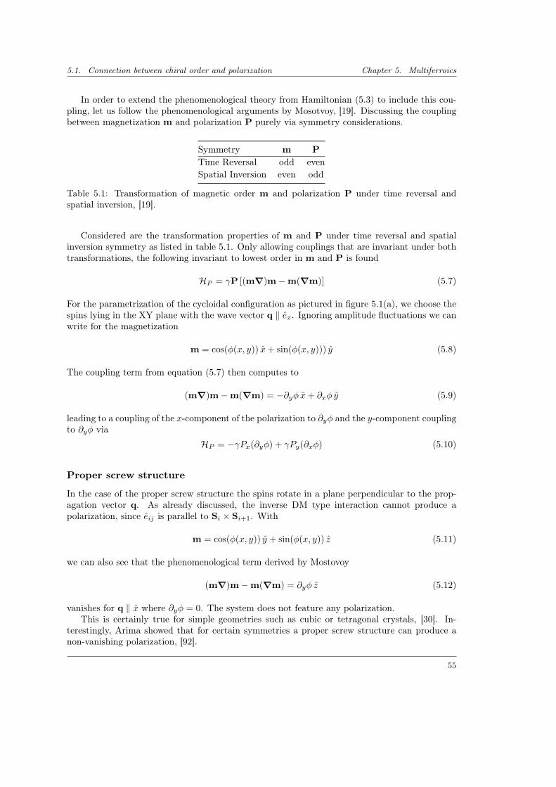
5.1. Connection between chiral order and polarization Chapter 5. Multiferroics

In order to extend the phenomenological theory from Hamiltonian (5.3) to include this cou-pling, let us follow the phenomenological arguments by Mosotvoy, [19]. Discussing the couplingbetween magnetization m and polarization P purely via symmetry considerations.

Symmetry m P

Time Reversal odd evenSpatial Inversion even odd

Table 5.1: Transformation of magnetic order m and polarization P under time reversal andspatial inversion, [19].

Considered are the transformation properties of m and P under time reversal and spatialinversion symmetry as listed in table 5.1. Only allowing couplings that are invariant under bothtransformations, the following invariant to lowest order in m and P is found

HP = γP [(m∇)m−m(∇m)] (5.7)

For the parametrization of the cycloidal configuration as pictured in figure 5.1(a), we choose thespins lying in the XY plane with the wave vector q ‖ ex. Ignoring amplitude fluctuations we canwrite for the magnetization

m = cos(φ(x, y)) x+ sin(φ(x, y))) y (5.8)

The coupling term from equation (5.7) then computes to

(m∇)m−m(∇m) = −∂yφ x+ ∂xφ y (5.9)

leading to a coupling of the x-component of the polarization to ∂yφ and the y-component couplingto ∂yφ via

HP = −γPx(∂yφ) + γPy(∂xφ) (5.10)

Proper screw structure

In the case of the proper screw structure the spins rotate in a plane perpendicular to the prop-agation vector q. As already discussed, the inverse DM type interaction cannot produce apolarization, since eij is parallel to Si × Si+1. With

m = cos(φ(x, y)) y + sin(φ(x, y)) z (5.11)

we can also see that the phenomenological term derived by Mostovoy

(m∇)m−m(∇m) = ∂yφ z (5.12)

vanishes for q ‖ x where ∂yφ = 0. The system does not feature any polarization.This is certainly true for simple geometries such as cubic or tetragonal crystals, [30]. In-

terestingly, Arima showed that for certain symmetries a proper screw structure can produce anon-vanishing polarization, [92].

55

Chapter 5. Multiferroics 5.2. One–dimensional domain wall

Effective theory

Assuming a cycloidal chiral ground state, we already derived the coupling to the polarization as

HP = γPy(∂xφ)− γPx(∂yφ) (5.13)

with the coupling constant γ. Together with the coupling EP to the electric field we get theeffective phenomenological theory

H =J

2

∫d2x

[1

4((∂xφ)2 − θ2)2 +

1

4(∂2xφ)2 + (∂yφ)2

]+

∫d2x

[γPy(∂xφ)− γPx(∂yφ)−EP +

P2

2χ+g

2(∇P)2

](5.14)

where χ is the dielectric susceptibility. Included is also a gradient term in (∇P)2 ≡∑i(∇Pi)2,allowed by the symmetry considerations.

Simple variation of the energy in respect to the polarization leads to

Py = χEy − χγ(∂xφ) + g∇2Py Px = χEx + χγ(∂yφ) + g∇2Px (5.15)

Connecting this to the vector order parameter

κ = 〈Si × Si+1〉 = 〈sin(∂xφ)〉κ (5.16)

where κ is perpendicular to the plane of rotation of the spins. For small q, i.e. small gradients,we can expand the sin(∂xφ) ≈ ∂xφ to see the direct connection to the polarization. Since 〈∂yφ〉vanishes as can be easily seen from the Hamiltonian, 〈P〉 and κ only differ in their orientation.The polarization in the absence of an external electric field is therefor directly related to theorder parameter of the chiral order. The helical spin liquid can therefor be identified via theabsence of magnetic order with a non vanishing polarization.

Measurement of polarization

Let us give some small notes on experimental methods to measure polarization. The measurementof a polarization perpendicular to the surface can be done by means of dielectric spectroscopy.This is achieved by placing the sample between two conducting layers forming a capacitor andapplying an alternating voltage, generating an electric field parallel to the polarization. Thepolarization of the sample changes its dielectric properties which changes the impedance of thecapacitor, leaving a measurable signature. A more elaborate technique even able to give spatialresolution of the domain walls in the system is the method of piezoresponse force microscopy(PFM), similar to atomic force microscopy with a electrically charged tip, described in detailin [95]. Using vertical or lateral movement of the tip allows the measurement of a polarizationperpendicular or parallel to the surface.

5.2 One–dimensional domain wall

Let us study the effect of the polarization and the coupling to the electric field on the groundstate and domain walls of the system in the x-direction. The effective one dimensional model ofthe chain in x-direction is then given by

Hx =J

2

∫dx

[1

4((∂xφ)2 − θ2)2 +

1

4(∂2xφ)2

]+

∫dx

[γPy(∂xφ)− EyPy +

P 2y

2χ+g

2(∂xPy)2

](5.17)

where we are only interested in electric fields that couple to the gradient in x-direction.

56

5.2. One–dimensional domain wall Chapter 5. Multiferroics

Ground state

The two functions of interest in the one–dimensional model are the pitch angle φ(x) of the spinsand the polarization profile Py(x) that minimize the energy Hx. Variation in respect to φ andPy leads to the two saddle point equations

δHxδφ

=J

2

((−3∂xφ)2∂2

xφ+ θ2∂2xφ+

1

2∂4xφ

)− γ∂xPy = 0 (5.18)

δHxδPy

=1

χPy − Ey + γ∂xφ− g∂2

xPy = 0 (5.19)

that can be simplified to

∂x

[J

2

((∂xφ)3 − θ2∂xφ−

1

2∂3xϕ

)+ γPy

]= 0 Py = χEy − χγ∂xφ+ gχ∂2

xPy (5.20)

Noting that these equations only depend on the gradients ∂xφ, we can use the substitutionΨ = ∂xφ and drop the index in Py for convenience,

2Ψ3 − 2θ2Ψ− ∂2xΨ +

4γ

JP = C P = χEy − χγΨ + gχ∂2

xP (5.21)

The integration constant C from the saddle point equations has the meaning of an applied electricfield. It can be absorbed by rescaling P → P + JC/(4γ) and Ey → Ey + JC/(4γχ). Afterabsorbing the integration constant we can look at minimum configuration of Ψ = Ψ0 = constand P = P0 = const with

2Ψ30 − 2θ2Ψ0 +

4γ

JP0 = 0 P0 = χEy − χγΨ0 (5.22)

leading to

2Ψ30 − 2

(θ2 +

2γ2χ

J

)Ψ0 +

4γχ

JEy = 0 (5.23)

For Ey = 0, this equation has two minima given by

Ψ0(Ey = 0) = ±√θ2 +

2γ2χ

J≡ ±θ (5.24)

The ground state solution Ψ0 = ∂xφ = const corresponds to a spiral with a fixed pitch angle θ.Here we can already see some effects of the coupling to the polarization via the constant γ. Oneis the new pitch angle θ > θ for γ 6= 0. The ground state value θ can be used to simplify theequations by rescaling θΨ0 = Ψ0 for Ey 6= 0. This leads to

Ψ30 − Ψ0 =

c

2c = − 4χγEy

J(θ2 + 2χγ2/J)3/2(5.25)

This cubic equation can be solved. We see (figure 5.2) that for |c| < cmax = 43√

3we have two

different minima, while for |c| > cmax only one minimum is selected due to the electric field. Thecritical field is given by

E(c)y =

J

χγ(3(θ2 + 2

χγ2

J))3/2 (5.26)

57

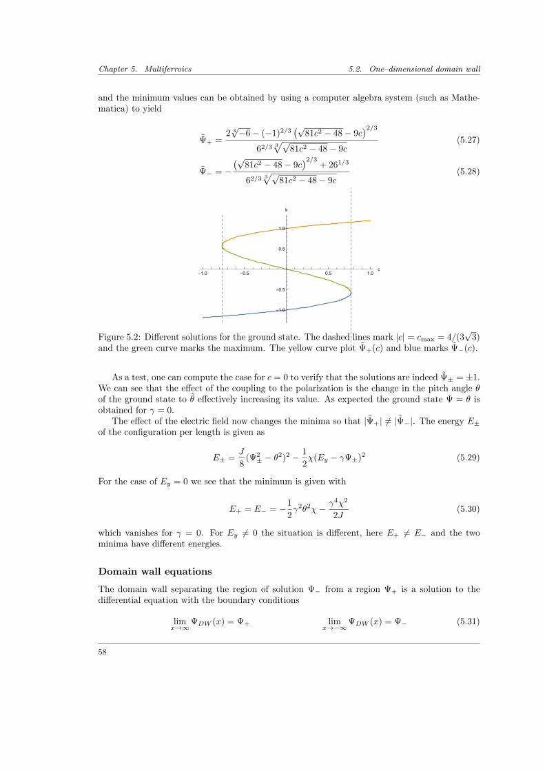
Chapter 5. Multiferroics 5.2. One–dimensional domain wall

and the minimum values can be obtained by using a computer algebra system (such as Mathe-matica) to yield

Ψ+ =2 3√−6− (−1)2/3

(√81c2 − 48− 9c

)2/362/3 3

√√81c2 − 48− 9c

(5.27)

Ψ− = −(√

81c2 − 48− 9c)2/3

+ 261/3

62/3 3√√

81c2 − 48− 9c(5.28)

-1.0 -0.5 0.5 1.0c

-1.0

-0.5

0.5

1.0

k

Figure 5.2: Different solutions for the ground state. The dashed lines mark |c| = cmax = 4/(3√

3)and the green curve marks the maximum. The yellow curve plot Ψ+(c) and blue marks Ψ−(c).

As a test, one can compute the case for c = 0 to verify that the solutions are indeed Ψ± = ±1.We can see that the effect of the coupling to the polarization is the change in the pitch angle θof the ground state to θ effectively increasing its value. As expected the ground state Ψ = θ isobtained for γ = 0.

The effect of the electric field now changes the minima so that |Ψ+| 6= |Ψ−|. The energy E±of the configuration per length is given as

E± =J

8(Ψ2± − θ2)2 − 1

2χ(Ey − γΨ±)2 (5.29)

For the case of Ey = 0 we see that the minimum is given with

E+ = E− = −1

2γ2θ2χ− γ4χ2

2J(5.30)

which vanishes for γ = 0. For Ey 6= 0 the situation is different, here E+ 6= E− and the twominima have different energies.

Domain wall equations

The domain wall separating the region of solution Ψ− from a region Ψ+ is a solution to thedifferential equation with the boundary conditions

limx→∞

ΨDW (x) = Ψ+ limx→−∞

ΨDW (x) = Ψ− (5.31)

58

5.2. One–dimensional domain wall Chapter 5. Multiferroics

In the absence of an electric field, we know Ψ+ = −Ψ− = θ and P± = −γχΨ±. The typicallength scale in this problem is given by the pitch angle θ. Using this information we can makethe saddle point equations

2Ψ3 − 2θ2Ψ− ∂2xΨ +

4γ

JP = 0 P = −χγΨ + gχ∂2

xP (5.32)

dimensionless, by introducing the rescaled functions ψ(x) and p(x) via

Ψ(x) = θψ(θx) P (x) = −γχθp(θx) (5.33)

The first equation transforms as

2θ3ψ3(θx)− 2θ2θψ(θx)− θ3∂2xψ(θx)− 4γ2χθ

Jp(θx) = 0

2θ3ψ3(θx)− 2 (θ2 +2γ2χ

J)︸ ︷︷ ︸

=θ2

θψ(θx)− θ3∂2xψ(θx) +

4γ2χθ

J(ψ(θx)− p(θx) = 0

2ψ3(θx)− 2ψ(θx)− ∂2xψ(θx) +

4γ2χ

Jθ2 (ψ(θx)− p(θx) = 0

The second equation can be written as

−γχθp(θx) = −χγθψ(θx)− gχ2γθ3∂2xp(x)

4γ2χ

Jθ2(ψ(θx)− p(θx)) = −4gγ2χ2

J∂2xp(θx)

After rescaling θx→ x we obtain the new saddle point equations

2ψ(x)3 − 2ψ(x)− ψ′′(x) + k(ψ(x)− p(x)) = 0 (5.34)lp′′(x) + k(ψ(x)− p(x)) = 0 (5.35)

making the saddle point equations only dependent on the parameters

k =4γ2χ

Jθ2and (5.36)

l = 4gγ2χ2/J. (5.37)

The energy in terms of ψ(x) and p(x) can be written as

Hx =J

8θ

∫dx

[(θ2ψ(x)2 − θ2)2 + θ4(∂xψ(x))2 +

4γ2χ

Jθ2(p(x)2 − 2p(x)ψ(x)

)+

4gθ4γ2χ2

J(∂xp(x))2

]

=Jθ3

8

∫dx

[(ψ(x)2 − 1)2 + (∂xψ(x))2 +

4γ2χ

Jθ2(p(x)− ψ(x))

2+

4gγ2χ2

J(∂xp(x))2

]+ const

Dropping the constant by shifting the ground state energy to zero and measuring the energy inunits of Jθ3/8 we obtain the dimensionless energy Hamiltonian of the form

H =

∫dx[(ψ(x)2 − 1)2 + (ψ′(x))2 + k (p(x)− ψ(x))

2+ l(p′(x))2

](5.38)

59

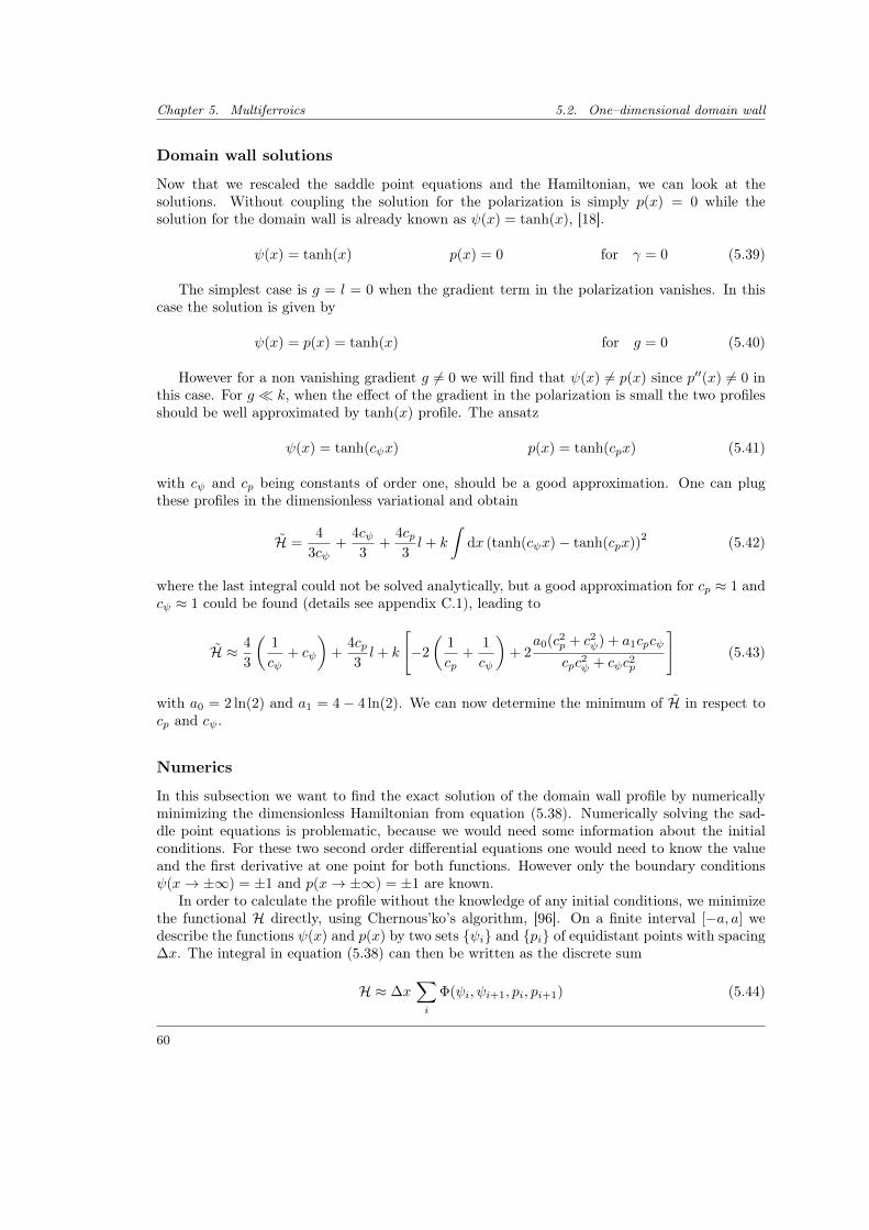
Chapter 5. Multiferroics 5.2. One–dimensional domain wall

Domain wall solutions

Now that we rescaled the saddle point equations and the Hamiltonian, we can look at thesolutions. Without coupling the solution for the polarization is simply p(x) = 0 while thesolution for the domain wall is already known as ψ(x) = tanh(x), [18].

ψ(x) = tanh(x) p(x) = 0 for γ = 0 (5.39)

The simplest case is g = l = 0 when the gradient term in the polarization vanishes. In thiscase the solution is given by

ψ(x) = p(x) = tanh(x) for g = 0 (5.40)

However for a non vanishing gradient g 6= 0 we will find that ψ(x) 6= p(x) since p′′(x) 6= 0 inthis case. For g k, when the effect of the gradient in the polarization is small the two profilesshould be well approximated by tanh(x) profile. The ansatz

ψ(x) = tanh(cψx) p(x) = tanh(cpx) (5.41)

with cψ and cp being constants of order one, should be a good approximation. One can plugthese profiles in the dimensionless variational and obtain

H =4

3cψ+

4cψ3

+4cp3l + k

∫dx (tanh(cψx)− tanh(cpx))

2 (5.42)

where the last integral could not be solved analytically, but a good approximation for cp ≈ 1 andcψ ≈ 1 could be found (details see appendix C.1), leading to

H ≈ 4

3

(1

cψ+ cψ

)+

4cp3l + k

[−2

(1

cp+

1

cψ

)+ 2

a0(c2p + c2ψ) + a1cpcψ

cpc2ψ + cψc2p

](5.43)

with a0 = 2 ln(2) and a1 = 4− 4 ln(2). We can now determine the minimum of H in respect tocp and cψ.

Numerics

In this subsection we want to find the exact solution of the domain wall profile by numericallyminimizing the dimensionless Hamiltonian from equation (5.38). Numerically solving the sad-dle point equations is problematic, because we would need some information about the initialconditions. For these two second order differential equations one would need to know the valueand the first derivative at one point for both functions. However only the boundary conditionsψ(x→ ±∞) = ±1 and p(x→ ±∞) = ±1 are known.

In order to calculate the profile without the knowledge of any initial conditions, we minimizethe functional H directly, using Chernous’ko’s algorithm, [96]. On a finite interval [−a, a] wedescribe the functions ψ(x) and p(x) by two sets ψi and pi of equidistant points with spacing∆x. The integral in equation (5.38) can then be written as the discrete sum

H ≈ ∆x∑i

Φ(ψi, ψi+1, pi, pi+1) (5.44)

60

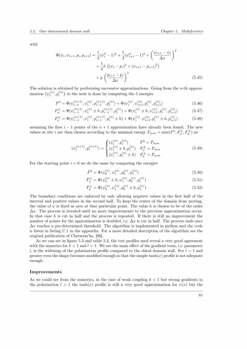
5.2. One–dimensional domain wall Chapter 5. Multiferroics

with

Φ(ψi, ψi+1, pi, pi+1) =1

2(ψ2i − 1)2 +

1

2(ψ2i+1 − 1)2 +

(ψi+1 − ψi

∆x

)2

+1

2k((ψi − pi)2 + (ψi+1 − pi+1)2

)+ g

(pi+1 − pi

∆x

)2

(5.45)

The solution is obtained by performing successive approximations. Going from the n-th approx-imation ψ(n)

i , p(n)i to the next is done by computing the 5 energies

F 0 = Φ(ψ(n+1)i−1 , ψ

(n)i , p

(n+1)i−1 , p

(n)i ) + Φ(ψ

(n)i , ψ

(n)i+1, p

(n)i , p

(n)i+1) (5.46)

F±ψ = Φ(ψ(n+1)i−1 , ψ

(n)i ± h, p(n+1)

i−1 , p(n)i ) + Φ(ψ

(n)i ± h, ψ(n)

i+1, p(n)i , p

(n)i+1) (5.47)

F±p = Φ(ψ(n+1)i−1 , ψ

(n)i , p

(n+1)i−1 , p

(n)i ± h) + Φ(ψ

(n)i , ψ

(n)i+1, p

(n)i ± h, p(n)

i+1) (5.48)

assuming the first i − 1 points of the n + 1 approximation have already been found. The newvalues at site i are then chosen according to the minimal energy Fmin = min(F 0, F±ψ , F

±p ) as

(ψ(n+1)i , p

(n+1)i ) =

(ψ

(n)i , p

(n)i ) F 0 = Fmin

(ψ(n)i ± h, p(n)

i ) F±ψ = Fmin

(ψ(n)i , p

(n)i ± h) F±p = Fmin

(5.49)

For the starting point i = 0 we do the same by comparing the energies

F 0 = Φ(ψ(n)0 , ψ

(n)1 , p

(n)0 , p

(n)1 ) (5.50)

F±ψ = Φ(ψ(n)0 ± h, ψ(n)

1 , p(n)0 , p

(n)i ) (5.51)

F±p = Φ(ψ(n)0 , ψ

(n)1 , p

(n)0 ± h, p(n)

1 ) (5.52)

The boundary conditions are enforced by only allowing negative values in the first half of theinterval and positive values in the second half. To keep the center of the domain from moving,the value of ψ is fixed as zero at that particular point. The value h is chosen to be of the order∆x. The process is iterated until no more improvements to the previous approximation occur.In that case h is cut in half and the process is repeated. If there is still no improvement thenumber of points for the approximation is doubled, i.e. ∆x is cut in half. The process ends once∆x reaches a pre-determined threshold. The algorithm is implemented in python and the codeis listen in listing C.1 in the appendix. For a more detailed description of the algorithm see theoriginal publication of Chernous’ko, [96].

As we can see in figure 5.3 and table 5.2, the test profiles used reveal a very good agreementwith the numerics for k < 1 and l < 1. We see the main effect of the gradient term, i.e. parameterl, is the widening of the polarization profile compared to the chiral domain wall. For l ∼ 1 andgreater even the shape becomes modified enough so that the simple tanh(x) profile is not adequateenough.

Improvements

As we could see from the numerics, in the case of weak coupling k < 1 but strong gradients inthe polarization l > 1 the tanh(x) profile is still a very good approximation for ψ(x) but the

61

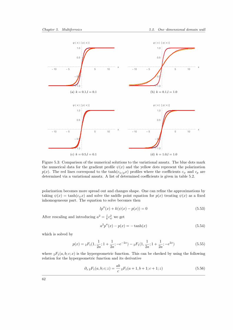
Chapter 5. Multiferroics 5.2. One–dimensional domain wall

- 10 - 5 5 10x

- 1.0

- 0.5

0.5

1.0

ψ ( x ) [ p ( x ) ]

(a) k = 0.1,l = 0.1

- 10 - 5 5 10x

- 1.0

- 0.5

0.5

1.0

ψ ( x ) [ p ( x ) ]

(b) k = 0.1,l = 1.0

- 10 - 5 5 10x

- 1.0

- 0.5

0.5

1.0

ψ ( x ) [ p ( x ) ]

(c) k = 0.5,l = 0.1

- 10 - 5 5 10x

- 1.0

- 0.5

0.5

1.0

ψ ( x ) [ p ( x ) ]

(d) k = 1.0,l = 1.0

Figure 5.3: Comparison of the numerical solutions to the variational ansatz. The blue dots markthe numerical data for the gradient profile ψ(x) and the yellow dots represent the polarizationp(x). The red lines correspond to the tanh(cψ/px) profiles where the coefficients cψ and cp aredetermined via a variational ansatz. A list of determined coefficients is given in table 5.2.

polarization becomes more spread out and changes shape. One can refine the approximations bytaking ψ(x) = tanh(cψx) and solve the saddle point equation for p(x) treating ψ(x) as a fixedinhomogeneous part. The equation to solve becomes then

lp′′(x) + k(ψ(x)− p(x)) = 0 (5.53)

After rescaling and introducing a2 = lk c

2ψ we get

a2p′′(x)− p(x) = − tanh(x) (5.54)

which is solved by

p(x) = 2F1(1,1

2a; 1 +

1

2a;−e−2x)− 2F1(1,

1

2a; 1 +

1

2a;−e2x) (5.55)

where 2F1(a, b; c;x) is the hypergeometric function. This can be checked by using the followingrelation for the hypergeometric function and its derivative

∂z 2F1(a, b; c; z) =ab

c2F1(a+ 1, b+ 1; c+ 1; z) (5.56)

62

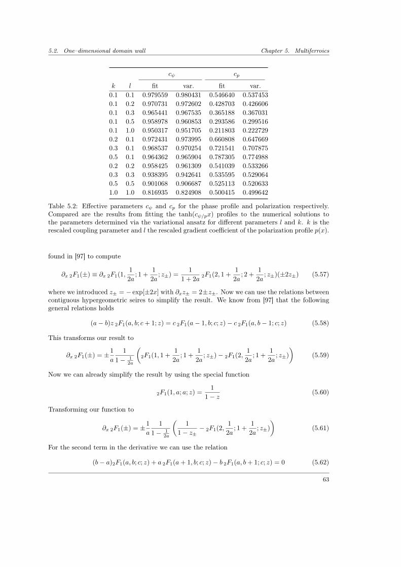
5.2. One–dimensional domain wall Chapter 5. Multiferroics

cψ cp

k l fit var. fit var.0.1 0.1 0.979559 0.980431 0.546640 0.5374530.1 0.2 0.970731 0.972602 0.428703 0.4266060.1 0.3 0.965441 0.967535 0.365188 0.3670310.1 0.5 0.958978 0.960853 0.293586 0.2995160.1 1.0 0.950317 0.951705 0.211803 0.2227290.2 0.1 0.972431 0.973995 0.660808 0.6476690.3 0.1 0.968537 0.970254 0.721541 0.7078750.5 0.1 0.964362 0.965904 0.787305 0.7749880.2 0.2 0.958425 0.961309 0.541039 0.5332660.3 0.3 0.938395 0.942641 0.535595 0.5290640.5 0.5 0.901068 0.906687 0.525113 0.5206331.0 1.0 0.816935 0.824908 0.500415 0.499642

Table 5.2: Effective parameters cψ and cp for the phase profile and polarization respectively.Compared are the results from fitting the tanh(cψ/px) profiles to the numerical solutions tothe parameters determined via the variational ansatz for different parameters l and k. k is therescaled coupling parameter and l the rescaled gradient coefficient of the polarization profile p(x).

found in [97] to compute

∂x 2F1(±) ≡ ∂x 2F1(1,1

2a; 1 +

1

2a; z±) =

1

1 + 2a2F1(2, 1 +

1

2a; 2 +

1

2a; z±)(±2z±) (5.57)

where we introduced z± = − exp[±2x] with ∂xz± = 2±z±. Now we can use the relations betweencontiguous hypergeometric seires to simplify the result. We know from [97] that the followinggeneral relations holds

(a− b)z 2F1(a, b; c+ 1; z) = c 2F1(a− 1, b; c; z)− c 2F1(a, b− 1; c; z) (5.58)

This transforms our result to

∂x 2F1(±) = ±1

a

1

1− 12a

(2F1(1, 1 +

1

2a; 1 +

1

2a; z±)− 2F1(2,

1

2a; 1 +

1

2a; z±)

)(5.59)

Now we can already simplify the result by using the special function

2F1(1, a; a; z) =1

1− z (5.60)

Transforming our function to

∂x 2F1(±) = ±1

a

1

1− 12a

(1

1− z±− 2F1(2,

1

2a; 1 +

1

2a; z±)

)(5.61)

For the second term in the derivative we can use the relation

(b− a)2F1(a, b; c; z) + a 2F1(a+ 1, b; c; z)− b 2F1(a, b+ 1; c; z) = 0 (5.62)

63

Chapter 5. Multiferroics 5.2. One–dimensional domain wall

also found in [97], leading to

2F1(2,1

2a; 1 +

1

2a; z±) = (1− 1

2a)2F1(1,

1

2a; 1 +

1

2a; z±) +

1

2a2F1(1, 1 +

1

2a; 1 +

1

2a; z±)

=1

2a

1

1− z±+ (1− 1

2a)2F1(1,

1

2a; 1 +

1

2a; z±) (5.63)

The derivative can then be written simply as

∂x 2F1(±) = ±1

a

(1

1− z±− 2F1(1,

1

2a; 1 +

1

2a; z±)

)(5.64)

The second derivative can now be performed easily and yields

∂2x 2F1(±) =

1

a

−z±(1− z±)2

− 1

a2

1

1− z±+

1

a2 2F1(±) (5.65)

Plugging this into the differential equation we get

(a2∂2x − 1)(2F1(−)− 2F1(+)) =

1

1− z+− 1

1− z−+

az+

(1− z+)2− az−

(1− z−)2

=1

1 + e2x− 1

1 + e−2x− ae2x

(1− e2x)2+− ae−2x

(1− e−2x)2

=1− e2x

1 + e2x= − tanh(x) (5.66)

So we have shown that the hypergeometric function is the solution to the inhomogeneous differ-ential equation.

The solution after beck transformation of the parameters is then

p(x) = 2F1(1,1

2cψ

√k

l; 1 +

1

2cψ

√k

l;−e−2xcψ )− 2F1(1,

1

2cψ

√k

l; 1 +

1

2cψ

√k

l;−e2xcψ ) (5.67)

Interaction potential of chiral domain wall and polarization domain wall

So far in the numerics we saw that ψ(x) and p(x) share the same center and thus are physicallylocated on top of each other. We now want to investigate this apparent one-to-one correspondencea bit further. As discussed above, the domain wall configuration is only stable in the absence ofan applied electric field. In the case of Ey = c = 0 and small parameters k and l the solution isgiven by

ψ(x) = tanh(cψx) p(x) = tanh(cpx) (5.68)

Now we look at the case where the profile of the phase gradient and the polarization are not atthe same position but separated by the distance ∆x by introducing

p(x−∆x) = tanh(cp(x−∆x)) (5.69)

Now we can compute an effective interaction potential V (∆x) for the two profiles as

V (∆x) = Hx[p(∆x)]−Hx[p(∆x = 0)] = 2k

∫dxψ(x)(p(x)− p(x−∆x)) (5.70)

64

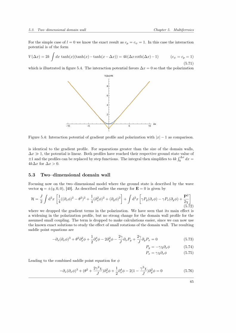
5.3. Two–dimensional domain wall Chapter 5. Multiferroics

For the simple case of l = 0 we know the exact result as cp = cψ = 1. In this case the interactionpotential is of the form

V (∆x) = 2k

∫dx tanh(x)(tanh(x)− tanh(x−∆x)) = 4k(∆x coth(∆x)−1) (cψ = cp = 1)

(5.71)which is illustrated in figure 5.4. The interaction potential favors ∆x = 0 so that the polarization

-10 -5 5 10Δx

2

4

6

8

V(Δx)/4k

Figure 5.4: Interaction potential of gradient profile and polarization with |x| − 1 as comparison.

is identical to the gradient profile. For separations greater than the size of the domain walls,∆x 1, the potential is linear. Both profiles have reached their respective ground state value of±1 and the profiles can be replaced by step functions. The integral then simplifies to 4k

∫∆x

0dx =

4k∆x for ∆x > 0.

5.3 Two–dimensional domain wall

Focusing now on the two–dimensional model where the ground state is described by the wavevector q = ±(q, 0, 0), [40]. As described earlier the energy for E = 0 is given by

H =J

2

∫d2x

[1

4((∂xφ)2 − θ2)2 +

1

4(∂2xφ)2 + (∂yφ)2

]+

∫d2x

[γPy(∂xφ)− γPx(∂yφ) +

P2

2χ

](5.72)

where we dropped the gradient terms in the polarization. We have seen that its main effect isa widening in the polarization profile, but no strong change for the domain wall profile for theassumed small coupling. The term is dropped to make calculations easier, since we can now usethe known exact solutions to study the effect of small rotations of the domain wall. The resultingsaddle point equations are

−∂x(∂xφ)3 + θ2∂2xφ+

1

2∂4xφ− 2∂2

yφ−2γ

J∂xPy +

2γ

J∂yPx = 0 (5.73)

Py = −γχ∂xφ (5.74)Px = γχ∂xφ (5.75)

Leading to the combined saddle point equation for φ

−∂x(∂xφ)3 + (θ2 +2γ2χ

J)∂2xφ+

1

2∂4xφ− 2(1− γ2χ

J)∂2yφ = 0 (5.76)

65

Chapter 5. Multiferroics 5.3. Two–dimensional domain wall

where J > γ22χ otherwise the gradient in ∂yφ contribution will diverge in the energy as we will

also see later when comparing the energies of different DW configurations. We can try to findsolutions of the form φ = f(z) with z = ax+ by reducing the equation to

−∂z(∂zf)3 +1

a4

[a2(θ2 +

2γ2χ

J)− 2b2(1− γ2χ

J)

]∂2zf +

1

2∂4zf = 0 (5.77)

Finally, we apply the rescaling

z 7→ d z (5.78)

d =1

a2

√a2(θ2 +

2γ2χ

J)− 2b2(1− γ2χ

J) (5.79)

a2 > b22(J − γ2χ)

Jθ2 + 2γ2χ(5.80)

where the inequality between the coefficients a and b ensures that we are still dealing with achiral minimum. A violation of that inequality removes the double minimum structure and weend up with the trivial φ = const ground state. After the rescaling we find

∂z

[−(∂zf)3 + ∂zf +

1

2∂2z (∂zf)

]= 0 (5.81)

which we already encountered and is solved by f(z) = ln(cosh(z)) + const leading to

φ = ln cosh

(1

a2

√a2(θ2 +

2γ2χ

J)− 2b2(1− γ2χ

J)(ax+ by)

)+ const (5.82)

The energy of the saddle point is given by

H =J

2

∫d2x

[1

4((∂xφ)2 − θ2)2 +

1

4(∂2xφ)2 − 1

Jγ2χ(∂xφ)2 + (1− 1

Jγ2χ)(∂yφ)2 − Emin

](5.83)

where the last term shifts the ground state energy to zero. Plugging the profile φ(a, b) in theequation we get an integral of the form∫

dx

∫dy f(ax+ by) (5.84)

where a rotation by α = arctan(b/a) transforms the integral to∫dx

∫dy f(

√a2 + b2x) = Ly

∫dx f(

√a2 + b2x) (5.85)

The domain wall energy is therefor proportional to its length. Doing the transformation afterplugging in φ(a, b) yields

H(a, b) = LxLyb2

2a4J

[(J − γ2χ

) (a2(2γ2χ+ θ2J

)+(γ2χ− J

))]+ Ly

1

4a4J

∫dx(a2(2γ2χ+ θ2J

)− 2b2

(J − γ2χ

))2×sech4

x√

(a2+b2)(a2(2γ2χ+θ2J)−2b2(J−γ2χ))J

a2

(5.86)

66

5.4. Domain wall in “four-state” model Chapter 5. Multiferroics

where on can easily see that any tilt in the domain wall, i.e. b 6= 0, is punished by an energyterm proportional to the area. The minimum solution is therefor b = 0 with

H(a, b = 0) =Jθ3

3Ly (5.87)

5.4 Domain wall in “four-state” model

Let us now consider a system where chiral order can also appear in the y-direction, leading to 4possible ground states of the form ±(q, q, 0) and ±(q,−q, 0). An easy way of constructing sucha model is by introducing a frustrated interaction in the y-direction, which leads to a simpleHamiltonian of the form

H(4) =J

8

∫d2x

[((∂xφ)2 − θ2)2 + (∂2

xφ)2 + ((∂yφ)2 − θ2)2 + (∂2yφ)2

](5.88)

with the saddle point equation

−∂x(∂xφ)3 + θ2∂2xφ+

1

2∂4xφ− ∂y(∂yφ)3 + θ2∂2

yφ+1

2∂4yφ = 0 (5.89)

Simple domain walls

To find solutions of single domain walls, i.e. walls separating two different domains, we use theansatz φ = f(z) with z = ax+by again, transforming the partial differential saddle point equationto an ordinary differential equation in z as

−∂z(∂zf)3 + θ2 a2 + b2

a4 + b4∂2zf +

1

2∂4zf = 0 (5.90)

yielding the solution

φ = ln(cosh(θ

√a2 + b2

a4 + b4(ax+ by))) (5.91)

where the the energy is given by

H = LxLyJθ4

8

(a2 − b2)2

(a4 + b4)

+Jθ4

4

(a2 + b2)2

(a4 + b4)

∫dx

∫dy sech4

(θ

√a2 + b2

a4 + b4(ax+ by)

)(5.92)

Showing an area dependent part scaling with (a2 − b2) vanishing for a = ±b, minimizing theenergy with E = 1

3Jθ3 L with L being the length of the domain wall. So the minimal energy

solution for the domain wall configurations separating two different domains is

φxy = ± ln(cosh(θ(x± y)) (5.93)

Domain walls separating 4 states

A simple extension to domain walls separating 4 domains can be found as

φV = ln(cosh(θx)) + ln(cosh(θy)) (5.94)φA = ln(cosh(θx))− ln(cosh(θy)) (5.95)

67

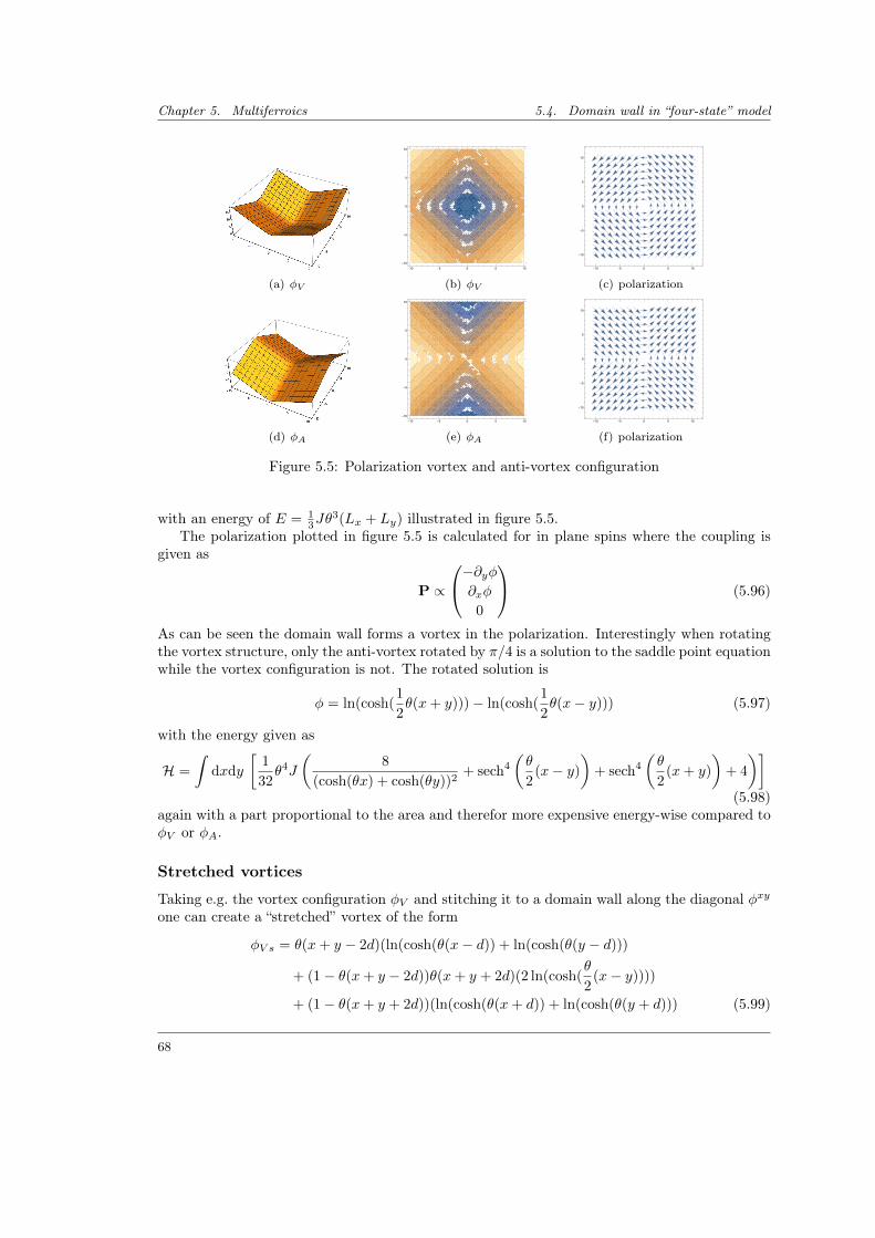
Chapter 5. Multiferroics 5.4. Domain wall in “four-state” model

(a) φV

-10 -5 0 5 10

-10

-5

0

5

10

(b) φV

-10 -5 0 5 10

-10

-5

0

5

10

(c) polarization

(d) φA

-10 -5 0 5 10

-10

-5

0

5

10

(e) φA

-10 -5 0 5 10

-10

-5

0

5

10

(f) polarization

Figure 5.5: Polarization vortex and anti-vortex configuration

with an energy of E = 13Jθ

3(Lx + Ly) illustrated in figure 5.5.The polarization plotted in figure 5.5 is calculated for in plane spins where the coupling is

given as

P ∝

−∂yφ∂xφ

0

(5.96)

As can be seen the domain wall forms a vortex in the polarization. Interestingly when rotatingthe vortex structure, only the anti-vortex rotated by π/4 is a solution to the saddle point equationwhile the vortex configuration is not. The rotated solution is

φ = ln(cosh(1

2θ(x+ y)))− ln(cosh(

1

2θ(x− y))) (5.97)

with the energy given as

H =

∫dxdy

[1

32θ4J

(8

(cosh(θx) + cosh(θy))2+ sech4

(θ

2(x− y)

)+ sech4

(θ

2(x+ y)

)+ 4

)](5.98)

again with a part proportional to the area and therefor more expensive energy-wise compared toφV or φA.

Stretched vortices

Taking e.g. the vortex configuration φV and stitching it to a domain wall along the diagonal φxyone can create a “stretched” vortex of the form

φV s = θ(x+ y − 2d)(ln(cosh(θ(x− d)) + ln(cosh(θ(y − d)))

+ (1− θ(x+ y − 2d))θ(x+ y + 2d)(2 ln(cosh(θ

2(x− y))))

+ (1− θ(x+ y + 2d))(ln(cosh(θ(x+ d)) + ln(cosh(θ(y + d))) (5.99)

68

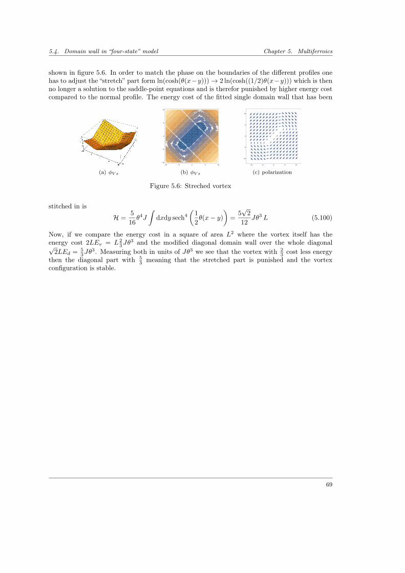
5.4. Domain wall in “four-state” model Chapter 5. Multiferroics

shown in figure 5.6. In order to match the phase on the boundaries of the different profiles onehas to adjust the “stretch” part form ln(cosh(θ(x−y)))→ 2 ln(cosh((1/2)θ(x−y))) which is thenno longer a solution to the saddle-point equations and is therefor punished by higher energy costcompared to the normal profile. The energy cost of the fitted single domain wall that has been

(a) φV s

-10 -5 0 5 10

-10

-5

0

5

10

(b) φV s

-10 -5 0 5 10

-10

-5

0

5

10

(c) polarization

Figure 5.6: Streched vortex

stitched in is

H =5

16θ4J

∫dxdy sech4

(1

2θ(x− y)

)=

5√

2

12Jθ3 L (5.100)

Now, if we compare the energy cost in a square of area L2 where the vortex itself has theenergy cost 2LEv = L 2

3Jθ3 and the modified diagonal domain wall over the whole diagonal√

2LEd = 53Jθ

3. Measuring both in units of Jθ3 we see that the vortex with 23 cost less energy

then the diagonal part with 53 meaning that the stretched part is punished and the vortex

configuration is stable.

69

6. MnWO4

In this chapter we will focus on the multiferroic material MnWO4. Here the chiral order couplesto the polarization, as indicated by a magnetic phase transition with an accompanied onset ofpolarization. In collaboration with D. Niermann and the group of Prof. J. Hemberger, the criticalbehavior of the phase transition was studied. First the different phase transitions in MnWO4 aredescribed and the crystal symmetry is discussed. Starting from the Ginzburg–Landau free energyexpansion done by Tolédano, the phase transitions will be classified and the critical dynamicalbehavior described. The resulting critical exponents are then compared to the experimental workof the group of Prof. J. Hemberger.

6.1 Material properties and observed phase transitions

MnWO4 crystallizes in the P2/c space group and shows three consecutive phase transitions.Starting from a paramagnetic phase P the system undergoes its first transition to an incommen-surate magnetic phase AF3 at TN = 13.4K over to an incommensurate elliptical spiral phaseAF2 at T2 = 12.6K featuring an electric polarization.

P TN−−→ AF3 T2−→ AF2 T1−→ COM

In the last transition the system goes over to a commensurate magnetic phase COM withoutelectric polarization AF1 at T1 = 6.8K,[37, 98, 99].

6.2 Group theory construction of Ginzburg–Landau free energy

The description of the phase transitions via the Ginzburg–Landau free energy has been donein [100]. Here we like to sketch the group theoretical method used to construct the free energybefore moving on to the classifications of the different phase transitions.

Group theory and symmetries

Concerned with the symmetry analysis of MnWO4, we start with the point group symmetry ofthe underlying Bravais lattice and will move on to the space group describing the crystal structureafterward. The Bravais lattice of MnWO4 is monoclinic, [98], with the lattice constants a 6= b 6= cand an easy axis b (β = 91.075)

a = 4.8226(3)Å b = 5.7533(6)Å c = 4.9923(5)Å

according to [98].The point group P for the monoclinic lattice of MnWO4 is P = C2h = 2/m and contains

all lattice symmetries leaving at least one point invariant. It consist of the identity 1, the 180degree rotation C2 around the easy-axis b (index n = 2 for 2π/n rotation), the mirror symmetryσ perpendicular to the rotation axis and the Inversion symmetry I.

P = 1, C2, σ, I (6.1)

71

Chapter 6. MnWO4 6.2. Group theory construction of Ginzburg–Landau free energy

creating the 4 equivalent points

(x, y, z) (x, y, z) (x, y, z) (x, y, z)

Moving to the space group S of the actual crystal structure we add the translation operatorsTa, Tb and Tc allowing for glide reflections (reflections followed by a translation) and screw axis(rotations followed by a translation along the rotation axis) in the crystal. As reported e.g. in[98] the space group of MnWO4 is P2/c which means that the mirror operation σ from thepoint group is followed by a displacement of half a lattice constant in c (T c

2) while the rotation

symmetry is left unchanged [101], leaving

S = 1, C2, T c2σ,C2T c2σ (6.2)

with the 4 equivalent points

(x, y, z) (x, y, z) (x, y, z + 1/2) (x, y, z − 1/2)

We see that the operator C2T c2 (x, y, z) = (x, y, z)− (0, 0, 1/2) is actually an inversion symmetrywith its center half way between the two points at −(0, 0, 1/4). The lattice is centrosymmetric(i.e. I ∈ P) and if we want to write the crystal structure as centrosymmetric it is convenientto shift the system by (0, 0, 1/4) to make the new inversion center (0, 0, 0). The glide reflectionσc = T c

2σ is not affected by this, but the rotation axis of C2 moves now through (0, 0, 1/4)

denoted by C2. The P2/c space group consists of

P2/c = 1, C2, σc, I (6.3)

producing the 4 equivalent points

(x, y, z) (x, y, z + 1/2) (x, y, z + 1/2) (x, y, z) (6.4)

which is the standard form of P2/c, [98].Now we have classified the crystal symmetry of MnWO4. For the study of the magnetic

phase transitions however, we are interested in all magnetic symmetries, classified by the so calledmagnetic group. The magnetic group or Shubnikov group describes all the symmetries that leavemagnetic structures invariant. Magnetic moments are inverted under time reversal symmetry R.When classifying magnetic symmetries one has to include the time reversal operator. Obviouslythe magnetic group cannot contain R itself. A magnetic structure that is symmetric in R wouldrequire that for each magnetic moment mi

mi = Rmi = −mi

holds. This is only satisfied vanishing magnetic moments mi = 0 in the system, describing anon-magnetic state. Group theoretically speaking we cannot just take the direct product of thespace group with the time reversal group 1, R. It is constructed as the direct product of thespace group P2/c with the time reversal symmetry R. There are 3 possible magnetic groupsbased on the point group P2/c, [101]. The magnetic group realized in MnWO4 is P2/c1’, [100].The prime indicates that the inversion symmetry is multiplied with the time reversal, while the2-rotation is not, meaning that

P2/c1’ = 1, C2, Rσc, RI (6.5)

A formal construction is done via the subgroup H = 1, C2 of index 2 = |P2/c|/|H|. It is knownfrom group theory that the construction

P2/c1’ = H+R(P2/c−H) (6.6)

forms a group, [101].

72

6.2. Group theory construction of Ginzburg–Landau free energy Chapter 6. MnWO4

Construction of free energy

In order to construct the free energy of the system, we have to identify the order parametersassociated with the group and then construct the invariants of the group. To do so we firstdetermine the irreducible representation of the magnetic space group P2/c1’. They can be foundin [102] or we can use Olbrychski’s method, [103], to determine the representation. For this weidentify the generators G of the space group, i.e. set of elements that form all elements in thegroup through multiplication.

G = σc, I, R, Ta, Tb, Tc (6.7)

where R is time reversal symmetry and Ti is the translation in i-direction according to theincommensurable wave-vector kinc = (kx, 1/2, kz) of the AF2 phase. Now we write down theabstract definition of the generators by writing down the relations between the generators. Thesequence of lattice translation is not important, so the operators Ti all commute with each other.Also it is not important if we first perform the translation to a certain lattice vector and thenapply time reversal or reverse time before doing the translation. Therefor we have

[Ti, Tj ] = 0 [R, Ti] = 0 i, j ∈ a, b, c. (6.8)

Additionally space inversion I and time reversal are their own inverse, leading to the two relations

I2 = 1 R2 = 1 (6.9)

Now we consider the relations between inversion I and translation Ti. Moving in one basisdirection Ti, inverting the crystal around its inversion center (000) is equivalent to moving in theopposite direction T−1

i after inversion, i.e.

ITi = T−1i I ⇒ TiITi = I. (6.10)

For the glide reflection σc only the translation in b-direction is effected, leading to

σcTa/c = Ta/cσc σcTb = T−1b σc (6.11)

Taking the combination of Iσc leading to the point (x, y, z−1/2) and σcI leading to (x, y, y+1/2)shows that they differ by a translation Tc leading to their defining relation

σcI = TcIσc (6.12)

Now that the equations (6.8)-(6.12) define the generators, we can solve these equation and findthe two irreducible representations as listed in table 6.1, where we also used the knowledge aboutthe translation subgroup discussed e.g. in [103–105].

The irreducible representation Γk1 and Γk2 have the two complex order parameters S1 =S1e

ıθ1 and S2 = S2eıθ2 associated with them. The transformations lead to the invariants I1 = S2

1 ,I2 = S2

2 and I3 = S1S1S∗2 S∗2 + S∗1 S

∗1 S2S2 ∝ S2

1S22 cos(2ϕ) with ϕ = θ1 − θ2, [100]. See appendix

D.1 for more details.The construction of the free energy from the invariants is straight forward

Φ(T, S1, S2, ϕ) = Φ10(T )+α1

2S2

1 +β1

4S4

1 +α2

2S2

2 +β2

4S4

2 +γ1

2S2

1S22 cos(2ϕ)+

γ2

4S4

1S42 cos2(2ϕ)+. . .

(6.13)Now we have to consider the coupling to the polarization Py, following the notation of Tolédano,[100]. As discussed in [19] time inversion leaves the polarization invariant RP = P while spaceinversion changes its sign, IP = −P . With this it is easy to see that Py(S1S

∗2 − S∗1 S2) ∝

73

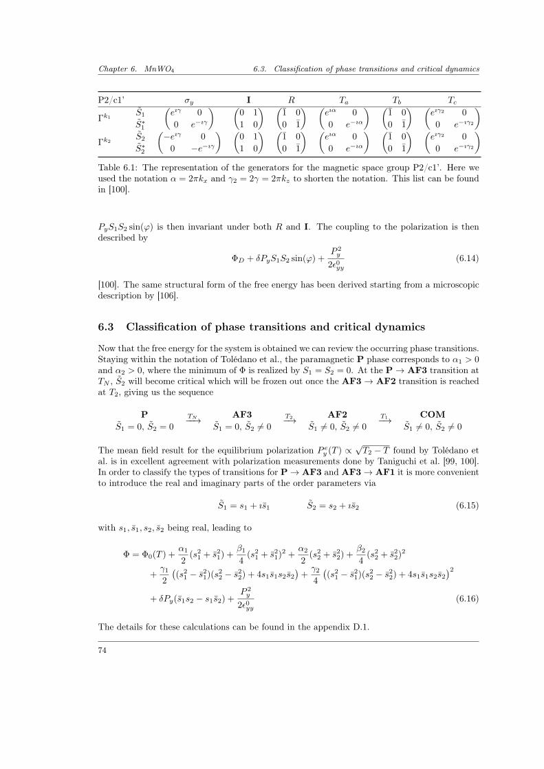
Chapter 6. MnWO4 6.3. Classification of phase transitions and critical dynamics

P2/c1’ σy I R Ta Tb Tc

Γk1S1

S∗1

(eıγ 0

0 e−ıγ

) (0 1

1 0

) (1 0

0 1

) (eıα 0

0 e−ıα

) (1 0

0 1

) (eıγ2 0

0 e−ıγ2

)Γk2

S2

S∗2

(−eıγ 0

0 −e−ıγ) (

0 1

1 0

) (1 0

0 1

) (eıα 0

0 e−ıα

) (1 0

0 1

) (eıγ2 0

0 e−ıγ2

)Table 6.1: The representation of the generators for the magnetic space group P2/c1’. Here weused the notation α = 2πkx and γ2 = 2γ = 2πkz to shorten the notation. This list can be foundin [100].

PyS1S2 sin(ϕ) is then invariant under both R and I. The coupling to the polarization is thendescribed by

ΦD + δPyS1S2 sin(ϕ) +P 2y

2ε0yy(6.14)

[100]. The same structural form of the free energy has been derived starting from a microscopicdescription by [106].

6.3 Classification of phase transitions and critical dynamics

Now that the free energy for the system is obtained we can review the occurring phase transitions.Staying within the notation of Tolédano et al., the paramagnetic P phase corresponds to α1 > 0and α2 > 0, where the minimum of Φ is realized by S1 = S2 = 0. At the P→ AF3 transition atTN , S2 will become critical which will be frozen out once the AF3 → AF2 transition is reachedat T2, giving us the sequence

PS1 = 0, S2 = 0

TN−−→ AF3S1 = 0, S2 6= 0

T2−→ AF2S1 6= 0, S2 6= 0

T1−→ COMS1 6= 0, S2 6= 0

The mean field result for the equilibrium polarization P ey (T ) ∝ √T2 − T found by Tolédano etal. is in excellent agreement with polarization measurements done by Taniguchi et al. [99, 100].In order to classify the types of transitions for P→ AF3 and AF3→ AF1 it is more convenientto introduce the real and imaginary parts of the order parameters via

S1 = s1 + ıs1 S2 = s2 + ıs2 (6.15)

with s1, s1, s2, s2 being real, leading to

Φ = Φ0(T ) +α1

2(s2

1 + s21) +

β1

4(s2

1 + s21)2 +

α2

2(s2

2 + s22) +

β2

4(s2

2 + s22)2

+γ1

2

((s2

1 − s21)(s2

2 − s22) + 4s1s1s2s2

)+γ2

4

((s2

1 − s21)(s2

2 − s22) + 4s1s1s2s2

)2+ δPy(s1s2 − s1s2) +

P 2y

2ε0yy(6.16)

The details for these calculations can be found in the appendix D.1.

74

6.3. Classification of phase transitions and critical dynamics Chapter 6. MnWO4

Transition from paramagnetic to commensurate phase (P → AF3)

At the transition P → AF3 at TN , the order parameter S2 is critical, i.e. α2 → 0 while α1 > 0.In this case the free energy in S1 is dominated by the quadratic part. Denoting the thermalaverage as 〈. . . 〉 we substitute the terms in s1 and s1 with their thermal averages. Assumingthat the components are not correlated and fluctuating according to the same distribution, afterintegrating out the polarization we get the resulting effective free energy

〈Φ〉 = Φ′0(T ) +α′22

(s22 + s2

2) +β′24

(s22 + s2

2)2 + ζs22s

22 (6.17)

with

α′2 = α2 − δ2ε0yy〈s21〉 β′2 = β2 + 2γ2(〈s4

1〉 − 〈s21〉2) ζ = 4γ2

(3〈s2

1〉2 − 〈s41〉)

(6.18)

where we see the correction to the transition temperature TN in α2 = a2(T − TN ) is of orderO(δ2) which is neglect able for small couplings δ as assumed by Tolédano et al., [100], and laterestimated by Matityahu et al. [106].

The model can be written as an O(N) model with cubic anisotropy with φ1 = s2 and φ2 = s2

and N = 2.

〈Φ〉 = g(T ) +m2

0

2

N∑i=1

φ2i +

u0

4!

(N∑i=1

φ2i

)2

+v0

4!

N∑i=1

(φ2i )

2 (6.19)

with the parameters

m20 = α′2 = α2 − δ2ε0yy〈s2

1〉 u0 = 6β′2 + 6γ′2

(1 +

ζ

2

)v0 = −3ζγ′2 γ′2 = 2γ2(〈s4

1〉 − 〈s21〉2)

(6.20)

An extended version of the calculation is done in section D.2. Assuming Gaussian fluctuationswe can use Wick’s theorem

〈s41〉 = 3〈s2

1〉2 (6.21)

which leads toζ = 0 ⇒ v0 = 0 (6.22)

a vanishing anisotropy term. The model is then identical to the O(2) model and the transitionlies in the 3D-XY universality class with the symmetric fixpoint being the stable one.

In the case of non-Gaussian fluctuations, we get a ζ 6= 0 and therefor an anisotropic term inthe O(2) model. This model has been studied for a sub critical N < Nc, where it has been foundthat the symmetric Heisenberg fixpoint is still the stable fixpoint for the system. There is stillsome debate on the exact value of Nc for d = 3, [107], which is in the order of Nc ∼ 3, howevercalculations by Aharony, [108, 109] and Brézin et.al [110] show that for N = 2 in d = 3 thesymmetric fix point is the stable one. The transition is then in the O(2)-symmetric universalityclass. The exponents up to O(ε5) and a discussion on the stability of the Heisenberg fix point inthe presents of cubic anisotropy is given in [91]. The same type of universality class for the P →AF3 transition has been discussed by Matityahu et al., [106] and the reference therein, Harriset al. [111].

Transition to the elliptical phase (AF3 → AF2)

For T < TN the order parameter S2 is frozen out, [100], and can be considered constant whenapproaching the second transition with α1 = a1(T − T2). The equilibrium value in S2 is given

75

Chapter 6. MnWO4 6.4. Dynamical exponent at AF3 → AF2

by S2 = s =√−α′2/β′2 with an arbitrary phase θ2 so that

s2 = s cos(θ2) s2 = s sin(θ2) (6.23)

Introducing the vector p = (s1, s1, Py) the quadratic part ΦM of the free energy with constants2 and s2 can be written as

ΦM =1

2pT M p (6.24)

with

M =

α1 + γ1s2 cos(2θ2) γ1s

2 sin(2θ2) −δs sin(θ2)

γ1s2 sin(2θ2) α1 − γ1s

2 cos(2θ2) δs cos(θ2)

−δs sin(θ2) δs cos(θ2) 1ε0yy

(6.25)

using cos2(θ2) − sin2(θ2) = cos(2θ2) and cos(θ2) sin(θ2) = 12 sin(2θ2). Even in the case of no

coupling to the polarization, i.e. δ = 0 we will see that only one component is becoming criticalat this transition, making it a member of the 3D-Ising universality class. For δ = 0 the eigenvaluesλi and eigenvectors vi of M can be obtained as

λ1 = α1 − γ1s2 λ2 = α1 + γ1s

2 λ3 =1

ε0yy(6.26)

and

v1 =

− sin(θ2)

cos(θ2)

0

v2 =

cos(θ2)

sin(θ2)

0

v3 =

0

0

1

(6.27)

As discussed in [100] the physical realized transition takes place for γ1 > 0. In that case λ1 isthe first eigenvalue to vanish, while the other two are still positive, so that only one componentbecomes critical. The phase transition is therefor in the O(1) 3D-Ising universality class, agreeingwith [106, 111]. A more detailed discussion is done in section D.3.

6.4 Dynamical exponent at AF3 → AF2

As seen in the previous section the transition at T2 lies in the 3D-Ising O(1) universality class.Using the vectors p = (s1, s1, Py) and the matrix M form equation (6.25) we could write thequadratic part of the free energy as pTMp. Now we want to rotate the system in its diagonalform with the new vector u = (u1, u2, u3) where only u1 becomes critical at T2. We determinethe eigenvalues and the corresponding eigenvectors leading to the construction of the rotationmatrix R that gives us the correspondence u ↔ p. We will order the eigenvalues in a way sothat λ1 corresponding to u1 is the first one to vanish, making u1 the critical field at T2. We get

λ1/2 =α1

2− γ1s

2

2+

1

2ε0yy∓ 1

2ε0yy

√4ε0yy

(s2(γ1 + δ2ε0yy

)− α1

)+(α1ε0yy − γ1s2ε0yy + 1

)2λ3 = α1 + γ1s

2

Here, the eigenvalues vanish at

α(1)1 = γ1s

2 + δ2ε0yy ⇒ λ1 = 0 (6.28)

α(2)1 = −γ1s

2 ⇒ λ3 = 0 (6.29)

76

6.4. Dynamical exponent at AF3 → AF2 Chapter 6. MnWO4

and λ2 never goes to zero. Expanding the eigenvalues around α(1)1 via α1 = α

(1)1 + x for small

deviation x around the critical value of α1 we get

λ1 =1

1 + s2δ2ε0yy2x+O(x2) (6.30)

λ2 =1

ε0yy+ s2δ2ε0yy + x

(1− 1

1 + s2δ2ε0yy2

)+O(x2) ≈ 1

ε0yy+ s2δ2ε0yy (6.31)

λ3 = 2γ1s2 + δ2ε0yy + x+O(x2) ≈ 2γ1s

2 + δ2ε0yy (6.32)

The eigenvectors vi can be written as

v1 =1√

B2 + 1

−B sin(θ1)

B cos(θ1)

1

v2 =1√

B2 + 1

sin(θ1)

− cos(θ1)

B

v3 =

cos(θ1)

sin(θ1)

0

(6.33)

Neither the rotated free energy nor the mapping Py(u) depends on the angle θ1 (as can be seeneither by doing the full calculations or by noting that the free energy is only dependent on theangle difference ϕ = θ1 − θ2). We can therefor choose θ1 = 0 to make the representations moreconvenient, leading to

v1 =1√

B2 + 1

0

B

1

v2 =1√

B2 + 1

0

−1

B

v3 =

1

0

0

(6.34)

with

B =1

2δsε0yy

√1 + ε

(−2α1 + ε0yy

((α1 − γ1s2)

2+ 4δ2s2

)+ 2γ1s2

)− α1

2δs+γ1s

2δ+

1

2δsε0yy

=1

sδε0yy− x

sδ + s3δ3ε0yy2 +O(x2) ≈ 1

sδε0yy(6.35)

where we expanded around α1 = α(1)1 + x and assumed small δ and temperatures close to the

transition. With this the rotation matrix becomes

R =1√

1 +B2

0 B 1

0 −1 B√1 +B2 0 0

(6.36)

And the relation for p↔ u

p =

s1

s1

Py

= RTu =1√

1 +B2

u3

√1 +B2

Bu1 − u2

u1 +Bu2

(6.37)

leading to the polarization

Py =1√

1 +B2(u1 +Bu2) (6.38)

For a spatial and time dependent polarization the fluctuations are

〈Py(x, t)Py(0)〉 =1

1 +B2(〈u1(x, t)u1(0)〉+ 2〈u1(x, t)u2(0)〉+ 〈u2(x, t)u2(0)〉) (6.39)

77

Chapter 6. MnWO4 6.4. Dynamical exponent at AF3 → AF2

At the transition point the fluctuations in u2 are still finite, so that the divergence in the po-larization is determined by the divergence in 〈u1(x, t)u1(0)〉, making their dynamical exponentsidentical. It is therefor sufficient to calculate the exponents for u1 in order to predict the expo-nents in the polarization fluctuation. Diagonalizing the free energy leads to

Φ =1

2λ1u

21 +

1

2λ2u

22 +

1

2λ3u

23 +

β+2

4

B4

(1 +B2)2u4

1 +β+

2

4

1

(1 +B2)2u4

2 +β+

2

4u4

3 +Aijui1uj2u

(4−i−j)3

(6.40)with β±2 = β2 ± γ2s

4 and A2,0, A1,1, A3,1, A0,2, A2,2, A1,3 being non-zero and the sum overdouble appearing indicies is applied.

A =1

1 +B2

0 0 B2

2 β−2 0

0 −Bβ−2 0 −B3β+

2

1+B2

12β−2 0

3B2β+2

2(1+B2) 0

0 − Bβ+2

1+B2 0 0

(6.41)

Close to λ1 = 0 the eigenvalues λ2 > 0 and λ3 > 0 with the quadratic terms in u2 and u3

dominate the behavior in these components. Substituting the values of u2 and u3 with theirthermal averages, one obtains a simple one-loop correction to the eigenvalue λ1 in an otherwisesimple φ4-theory model, Φu.

Φu = h(T ) +1

2λ′1u

21 +

β+2

4

B4

(1 +B2)2u4

1 λ′1 = λ1 +A2,0〈u23〉+A2,2〈u2

2〉 (6.42)

Leaving us with a simple φ4 theory at the transition T2. So now we want to consider the dynamicalscaling of an Ising order parameter. Assuming an overdamped dynamics with a dampeningcoefficient Γ0 our model is identical to the Model A discussed in [112]. The dynamical exponentz for the inverse relaxation time ω = τ−1 is

ω ∝ ξ−z ∝ tνz =

[T − T2

T2

]νz(6.43)

where νz is the experimentally measured exponent, at the reduced temperature t = (T −T2)/T2.Here ν is the critical exponent of the correlation length ξ of the 3D-Ising universality class.A good overview of the calculated exponents z for the 3D-Ising model is contained in Folk etal. [113], where the highest expansion is done by Prudnikov et al. [114] in terms of a 4-loop εexpansion with Padé-Borel summation leading to

z = 2.017 (6.44)

which is very good agreement with the numerically found values around z ≈ 2.02 found by [115–117]. With the value of ν found using resummation techniques (for d = 3) done by Guida andZinn–Justin [118]

ν = 0.6304± 0.0013 (6.45)

we get for the dynamical exponent of the relaxation time

νz ≈ 1.272 (6.46)

which is in agreement with the measured value νz ≈ 1.3, [41]. In accordance with the exper-imental observations this paints the picture that the critical dynamics of the polarization aredetermined by an overdamped magnetic 3D-Ising order parameter.

78

6.5. Discussion Chapter 6. MnWO4

6.5 Discussion

Using Bertraut’s group theoretical consideration, [104, 105] the Landau expansion of the freeenergy of MnWO4 was calculated. This was done following Tolédano et al., [100] for the incom-mensurable phase kinc = (−0.214, 1/2, 0.457), [98, 100]. This theory could be used to classifythe universality classes of the occurring transitions. The first transition form the paramagneticP phase to the incommensurable phase AF3 at TN was found to be in the 3D-XY universalityclass, in agreement with [106, 111]. The main interest however lies on the second transition atT2, where the incommensurable phase switches to the spiral phase AF2 with a non-vanishingpolarization Py 6= 0. The transition was found to be in the 3D-Ising universality class, agreeingwith [106, 111]. Describing the dynamics of the order parameter at the transition as overdampedleads to the so called Model A description, [112] and to a dynamical exponent νz ≈ 1.272 forMnWO4, agreeing with the measurements done by Niermann et al., [41]. The results of thischapter have been partially published in [41].

79

Part II

Vortices in Supraconducting Thin Films

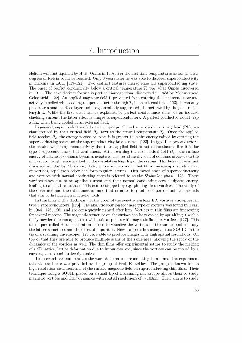
7. Introduction

Helium was first liquified by H. K. Onnes in 1908. For the first time temperatures as low as a fewdegrees of Kelvin could be reached. Only 3 years later he was able to discover superconductivityin mercury in 1911, [119–121]. Two distinct features characterize the superconducting state.The onset of perfect conductivity below a critical temperature Tc was what Onnes discoveredin 1911. The next distinct feature is perfect diamagnetism, discovered in 1933 by Meissner andOchsenfeld, [122]. An applied magnetic field is prevented from entering the superconductor andactively expelled while cooling a superconductor through Tc in an external field, [123]. It can onlypenetrate a small surface layer and is exponentially suppressed, characterized by the penetrationlength λ. While the first effect can be explained by perfect conductance alone via an inducedshielding current, the latter effect is unique to superconductors. A perfect conductor would trapa flux when being cooled in an external field.

In general, superconductors fall into two groups. Type I superconductors, e.g. lead (Pb), arecharacterized by their critical field Hc, next to the critical temperature Tc. Once the appliedfield reaches Hc, the energy needed to expel it is greater than the energy gained by entering thesuperconducting state and the superconductivity breaks down, [123]. In type II superconductors,the breakdown of superconductivity due to an applied field is not discontinuous like it is fortype I superconductors, but continuous. After reaching the first critical field Hc1 , the surfaceenergy of magnetic domains becomes negative. The resulting division of domains proceeds to themicroscopic length scale marked by the correlation length ξ of the system. This behavior was firstdiscussed in 1957 by Abrikosov, [124], who also discovered that these microscopic subdomains,or vortices, repel each other and form regular lattices. This mixed state of superconductivityand vortices with normal conducting cores is referred to as the Shubnikov phase, [123]. Thesevortices move due to an applied current and their normal conducting core dissipates energy,leading to a small resistance. This can be stopped by e.g. pinning these vortices. The study ofthese vortices and their dynamics is important in order to produce superconducting materialsthat can withstand high magnetic fields.

In thin films with a thickness d of the order of the penetration length λ, vortices also appear intype I superconductors, [123]. The analytic solution for these type of vortices was found by Pearlin 1964, [125, 126], and are consequently named after him. Vortices in thin films are interestingfor several reasons. The magnetic structure on the surface can be revealed by sprinkling it with afinely powdered ferromagnet that will settle at points with magnetic flux, i.e. vortices, [127]. Thistechniques called Bitter decoration is used to visualize the vortices on the surface and to studythe lattice structures and the effect of impurities. Newer approaches using a nano-SQUID on thetip of a scanning microscope, [128], are able to produce images with high spatial resolutions. Ontop of that they are able to produce multiple scans of the same area, allowing the study of thedynamics of the vortices as well. The thin films offer experimental setups to study the meltingof a 2D lattice, lattice deformation due to impurities and, since the vortices can be moved by acurrent, vortex and lattice dynamics.

This second part summarizes the work done on superconducting thin films. The experimen-tal data used here was provided by the group of Prof. E. Zeldov. The group is known for itshigh resolution measurements of the surface magnetic field on superconducting thin films. Theirtechnique using a SQUID placed on a small tip of a scanning microscope allows them to studymagnetic vortices and their dynamics with spatial resolutions of ∼ 100nm. Their aim is to study

83

Chapter 7. Introduction Chapter 7. Introduction

the movement of vortex lattices in order to study the moving Bragg–glass phase experimen-tally, [129–131]. The Bragg-glass phase is characterized by a power–law decay in the densitycorrelations.

At the beginning of the collaboration, the experiments were in their early stages. The mainidea was to focus on thin strips with differently sized constrictions. These constrictions introducesome inhomogeneities in the current profile and consequently cause inhomogeneous deformationsof the lattice. The deformed lattices with destroyed long-range correlation (no fixed latticestructure), are then moved by applying a direct current to the sample. When moving vorticesthrough the setup, several effects have to be taken into account. Vortices can enter the samplefrom the boarders of the strip and impurities can pin them.

We tried to contribute to the explanation of two different observed effects in their setups.Once a certain critical current Ic was surpassed, the vortices were observed to be moving, causinga measurable resistance. The measured V (I) curve on these strip setups was characterized by apower law behavior

V (I) ∼ Iα, α ∼ 10. (7.1)

We tried to understand the origin of the exponent α as an effect of vortices trying to overcome asurface barrier. The results and details are discussed in chapter 10. The second effect the groupobserved concerned the dynamics of the vortices. They noticed that the moving vortices formedlines, effectively following each other. Additionally, around the inhomogeneities caused by theconstrictions in the superconducting strip, these flow lines bifurcated. Both, the line formationand the origin of the bifurcation points are discussed in chapter 11.

Outline

We start by presenting the experimental setup and measurements that are the basis for theanalytic work in chapter 8. Here, the two different observed effects are described in detail. Afteran introduction to superconductivity, thin films and vortices in chapter 9, the work done on theobserved V (I) curves is discussed in chapter 10. This is followed by the presentation of the workdone on the vortex dynamics in chapter 11. The two projects are fairly separate, so an individualdiscussion is done at the end of each chapter.

84

8. Experimental Data

In this chapter we will focus on the experimental setup used by our collaborators L. Embon andE. Zeldov and the data they provided. There are two distinct features that we try to explain inthe following chapters and we want to set the stage for them here. The first section will coverthe setup and measurement techniques to give a general overview of the setup we are dealingwith. They use a technique called nanoSQUID microscopy to track superconducting vortices inthin films exposed to an applied current and measure the resulting voltage drop along the strips.First, we will present the current–voltage curves and their power–law behavior. Later, in chapter10, we will try and give an analytic explanation for this behavior. The moving vortices are alsoobserved to move in lines. This second feature will be presented here discussed in detail later inchapter 11.

8.1 Experimental setup

The dynamic properties of superconducting vortices in a thin type I superconductor are studiedexperimentally by our collaborators. The material used is a thin lead (Pb) film of thicknessd = 50nm that is capped by a thin ∼ 10nm Germanium (Ge) layer, to prevent oxidation. A listof material properties of lead assembled from literature is found in table E.1 in appendix E.1. Themask used in shown in figure 8.1, where the light gray areas resemble the lead film. It contains6 different strip setups, each with a different width for the hour-glass shaped constriction, [132].The strip width is w = 10µm for all setups, while the hourglass constriction can be as narrowas 5− 6µm. All measurements are done at T = 4.2K in a liquid Helium cryostat. The magneticfield H is applied perpendicular to the film. Gold contacts on the film are used to connect thewiring, schematically shown in figure 8.2. There are two contributions to the current that is fedinto the strip. The DC current is generated by applying a voltage UDC over an RDC = 566Ωresistor in series with the strip. Additionally a fixed AC contribution is added via a square waveUAC applied over a RAC = 10kΩ. The AC voltage signal is a square wave at 1.137kHz witha constant 1.2V amplitude. DC and AC part of the resulting voltage drop are measured by asimple voltmeter and a lock–in amplifier respectively, [132]. The small structures one can seein figure 8.1 and even better in figure 8.2 (circular pattern), are present for engineering reasonsonly. They do not influence the measurements done on the thin strips.

The measurements of the magnetic fields are done with a technique referred to as scanningSQUID microscopy. A small hollow quartz tube with an opening diameter of ∼ 200nm is usedand aluminum is evaporated on two opposing sides and on the circular opening, as illustrated in8.3. The aluminum on the two sides form superconducting leads connected to the nanoSQUIDring formed on the opening of the quartz tube. This structure is referred to as a SQUID on top(SOT), [128]. The SOT is used as the tip on a scanning microscope. This setup allows for a highspatial resolution when imaging the magnetic field on the surface of the superconducting thinfilms. With this it is possible to see the vortex distribution and even dynamics in the thin films.

85

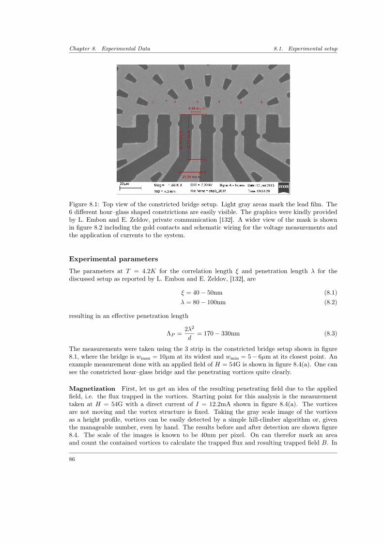
Chapter 8. Experimental Data 8.1. Experimental setup

Figure 8.1: Top view of the constricted bridge setup. Light gray areas mark the lead film. The6 different hour–glass shaped constrictions are easily visible. The graphics were kindly providedby L. Embon and E. Zeldov, private communication [132]. A wider view of the mask is shownin figure 8.2 including the gold contacts and schematic wiring for the voltage measurements andthe application of currents to the system.

Experimental parameters

The parameters at T = 4.2K for the correlation length ξ and penetration length λ for thediscussed setup as reported by L. Embon and E. Zeldov, [132], are

ξ = 40− 50nm (8.1)λ = 80− 100nm (8.2)

resulting in an effective penetration length

ΛP =2λ2

d= 170− 330nm (8.3)

The measurements were taken using the 3 strip in the constricted bridge setup shown in figure8.1, where the bridge is wmax = 10µm at its widest and wmin = 5− 6µm at its closest point. Anexample measurement done with an applied field of H = 54G is shown in figure 8.4(a). One cansee the constricted hour–glass bridge and the penetrating vortices quite clearly.

Magnetization First, let us get an idea of the resulting penetrating field due to the appliedfield, i.e. the flux trapped in the vortices. Starting point for this analysis is the measurementtaken at H = 54G with a direct current of I = 12.2mA shown in figure 8.4(a). The vorticesare not moving and the vortex structure is fixed. Taking the gray scale image of the vorticesas a height profile, vortices can be easily detected by a simple hill-climber algorithm or, giventhe manageable number, even by hand. The results before and after detection are shown figure8.4. The scale of the images is known to be 40nm per pixel. On can therefor mark an areaand count the contained vortices to calculate the trapped flux and resulting trapped field B. In

86

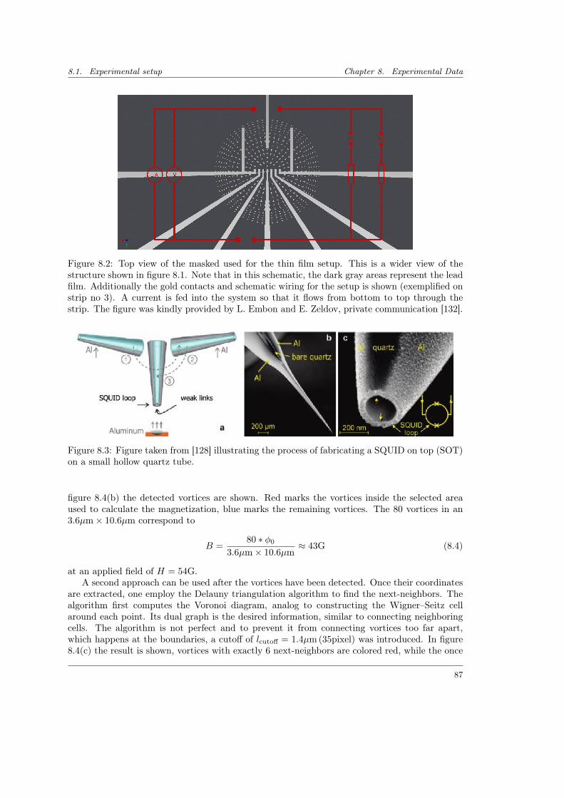
8.1. Experimental setup Chapter 8. Experimental Data

Figure 8.2: Top view of the masked used for the thin film setup. This is a wider view of thestructure shown in figure 8.1. Note that in this schematic, the dark gray areas represent the leadfilm. Additionally the gold contacts and schematic wiring for the setup is shown (exemplified onstrip no 3). A current is fed into the system so that it flows from bottom to top through thestrip. The figure was kindly provided by L. Embon and E. Zeldov, private communication [132].

Figure 8.3: Figure taken from [128] illustrating the process of fabricating a SQUID on top (SOT)on a small hollow quartz tube.

figure 8.4(b) the detected vortices are shown. Red marks the vortices inside the selected areaused to calculate the magnetization, blue marks the remaining vortices. The 80 vortices in an3.6µm× 10.6µm correspond to

B =80 ∗ φ0

3.6µm× 10.6µm≈ 43G (8.4)

at an applied field of H = 54G.A second approach can be used after the vortices have been detected. Once their coordinates

are extracted, one employ the Delauny triangulation algorithm to find the next-neighbors. Thealgorithm first computes the Voronoi diagram, analog to constructing the Wigner–Seitz cellaround each point. Its dual graph is the desired information, similar to connecting neighboringcells. The algorithm is not perfect and to prevent it from connecting vortices too far apart,which happens at the boundaries, a cutoff of lcutoff = 1.4µm (35pixel) was introduced. In figure8.4(c) the result is shown, vortices with exactly 6 next-neighbors are colored red, while the once

87

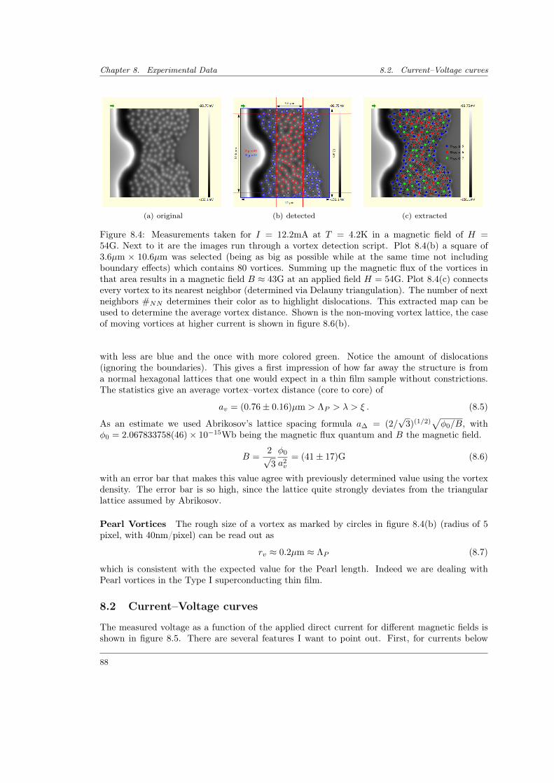
Chapter 8. Experimental Data 8.2. Current–Voltage curves

(a) original (b) detected (c) extracted

Figure 8.4: Measurements taken for I = 12.2mA at T = 4.2K in a magnetic field of H =54G. Next to it are the images run through a vortex detection script. Plot 8.4(b) a square of3.6µm × 10.6µm was selected (being as big as possible while at the same time not includingboundary effects) which contains 80 vortices. Summing up the magnetic flux of the vortices inthat area results in a magnetic field B ≈ 43G at an applied field H = 54G. Plot 8.4(c) connectsevery vortex to its nearest neighbor (determined via Delauny triangulation). The number of nextneighbors #NN determines their color as to highlight dislocations. This extracted map can beused to determine the average vortex distance. Shown is the non-moving vortex lattice, the caseof moving vortices at higher current is shown in figure 8.6(b).

with less are blue and the once with more colored green. Notice the amount of dislocations(ignoring the boundaries). This gives a first impression of how far away the structure is froma normal hexagonal lattices that one would expect in a thin film sample without constrictions.The statistics give an average vortex–vortex distance (core to core) of

av = (0.76± 0.16)µm > ΛP > λ > ξ . (8.5)

As an estimate we used Abrikosov’s lattice spacing formula a∆ = (2/√

3)(1/2)√φ0/B, with

φ0 = 2.067833758(46)× 10−15Wb being the magnetic flux quantum and B the magnetic field.

B =2√3

φ0

a2v

= (41± 17)G (8.6)

with an error bar that makes this value agree with previously determined value using the vortexdensity. The error bar is so high, since the lattice quite strongly deviates from the triangularlattice assumed by Abrikosov.

Pearl Vortices The rough size of a vortex as marked by circles in figure 8.4(b) (radius of 5pixel, with 40nm/pixel) can be read out as

rv ≈ 0.2µm ≈ ΛP (8.7)

which is consistent with the expected value for the Pearl length. Indeed we are dealing withPearl vortices in the Type I superconducting thin film.

8.2 Current–Voltage curves

The measured voltage as a function of the applied direct current for different magnetic fields isshown in figure 8.5. There are several features I want to point out. First, for currents below

88

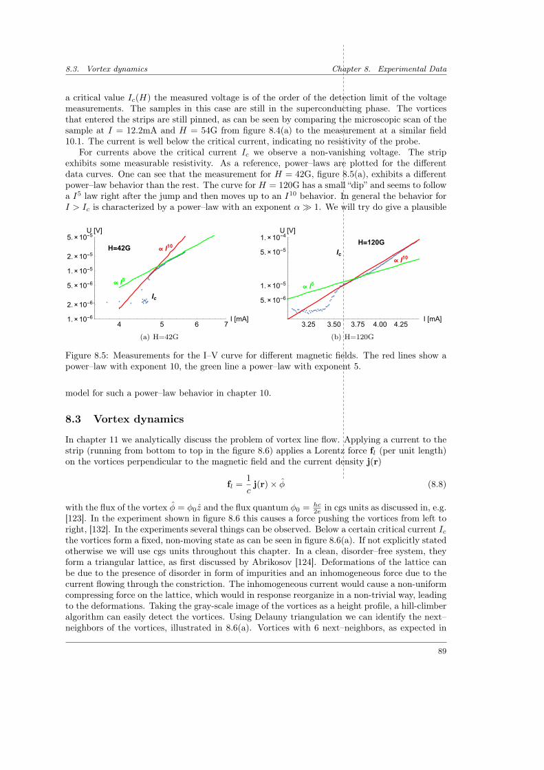
8.3. Vortex dynamics Chapter 8. Experimental Data

a critical value Ic(H) the measured voltage is of the order of the detection limit of the voltagemeasurements. The samples in this case are still in the superconducting phase. The vorticesthat entered the strips are still pinned, as can be seen by comparing the microscopic scan of thesample at I = 12.2mA and H = 54G from figure 8.4(a) to the measurement at a similar field10.1. The current is well below the critical current, indicating no resistivity of the probe.

For currents above the critical current Ic we observe a non-vanishing voltage. The stripexhibits some measurable resistivity. As a reference, power–laws are plotted for the differentdata curves. One can see that the measurement for H = 42G, figure 8.5(a), exhibits a differentpower–law behavior than the rest. The curve for H = 120G has a small “dip” and seems to followa I5 law right after the jump and then moves up to an I10 behavior. In general the behavior forI > Ic is characterized by a power–law with an exponent α 1. We will try do give a plausible

4 5 6 7I [mA]1.×10-6

2.×10-6

5.×10-6

1.×10-5

2.×10-5

5.×10-5U [V]

H=42G ∝ I10

∝ I5

Ic

(a) H=42G

3.25 3.50 3.75 4.00 4.25I [mA]

5.×10-6

1.×10-5

5.×10-5

1.×10-4U [V]

H=120GIc

∝ I10

∝ I5

(b) H=120G

Figure 8.5: Measurements for the I–V curve for different magnetic fields. The red lines show apower–law with exponent 10, the green line a power–law with exponent 5.

model for such a power–law behavior in chapter 10.

8.3 Vortex dynamics

In chapter 11 we analytically discuss the problem of vortex line flow. Applying a current to thestrip (running from bottom to top in the figure 8.6) applies a Lorentz force fl (per unit length)on the vortices perpendicular to the magnetic field and the current density j(r)

fl =1

cj(r)× φ (8.8)

with the flux of the vortex φ = φ0z and the flux quantum φ0 = hc2e in cgs units as discussed in, e.g.

[123]. In the experiment shown in figure 8.6 this causes a force pushing the vortices from left toright, [132]. In the experiments several things can be observed. Below a certain critical current Icthe vortices form a fixed, non-moving state as can be seen in figure 8.6(a). If not explicitly statedotherwise we will use cgs units throughout this chapter. In a clean, disorder–free system, theyform a triangular lattice, as first discussed by Abrikosov [124]. Deformations of the lattice canbe due to the presence of disorder in form of impurities and an inhomogeneous force due to thecurrent flowing through the constriction. The inhomogeneous current would cause a non-uniformcompressing force on the lattice, which would in response reorganize in a non-trivial way, leadingto the deformations. Taking the gray-scale image of the vortices as a height profile, a hill-climberalgorithm can easily detect the vortices. Using Delauny triangulation we can identify the next–neighbors of the vortices, illustrated in 8.6(a). Vortices with 6 next–neighbors, as expected in

89

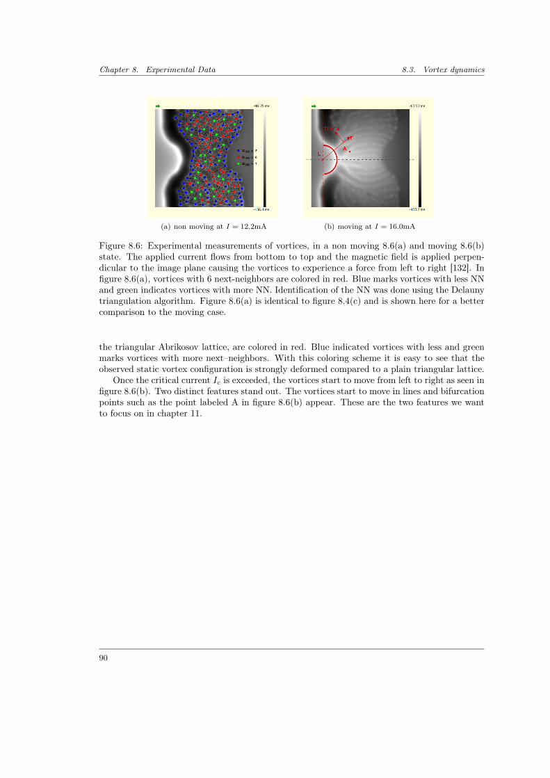
Chapter 8. Experimental Data 8.3. Vortex dynamics

(a) non moving at I = 12.2mA (b) moving at I = 16.0mA

Figure 8.6: Experimental measurements of vortices, in a non moving 8.6(a) and moving 8.6(b)state. The applied current flows from bottom to top and the magnetic field is applied perpen-dicular to the image plane causing the vortices to experience a force from left to right [132]. Infigure 8.6(a), vortices with 6 next-neighbors are colored in red. Blue marks vortices with less NNand green indicates vortices with more NN. Identification of the NN was done using the Delaunytriangulation algorithm. Figure 8.6(a) is identical to figure 8.4(c) and is shown here for a bettercomparison to the moving case.

the triangular Abrikosov lattice, are colored in red. Blue indicated vortices with less and greenmarks vortices with more next–neighbors. With this coloring scheme it is easy to see that theobserved static vortex configuration is strongly deformed compared to a plain triangular lattice.

Once the critical current Ic is exceeded, the vortices start to move from left to right as seen infigure 8.6(b). Two distinct features stand out. The vortices start to move in lines and bifurcationpoints such as the point labeled A in figure 8.6(b) appear. These are the two features we wantto focus on in chapter 11.

90

9. Superconductivity

This chapter will give a brief introduction into the theoretical description of superconductivitywith the focus on superconducting vortices. A successful microscopic theory for superconductivitywas developed by Bardeen, Cooper and Schrieffer in 1957, [133] , commonly referred to as theBCS theory of superconductivity. The basic idea behind the theory is that electrons form socalled Cooper-pairs due to an attractive interaction cause by lattice deformations (phonons).These pairs of electrons are now of bosonic nature and can all occupy the same groundstate,forming the quantum state that is superconductivity. Despite its importance, we will not focuson the microscopic picture since the work done on superconductors in this part is based on theearlier macroscopic and phenomenological description by the Ginzburg–Landau theory and theLondon equations.

London–Equations

One of the first phenomenological descriptions of superconductivity was done by F. and H. Lon-don, [134], by proposing the two equations

E = Λ∂

∂tjs (9.1)

B = −cΛ∇× js (9.2)

for the microscopic electric field E, magnetic field B and the superconducting current js. Here

Λ =4πλ2

c2=

m

nse2(9.3)

was introduced as a phenomenological parameter, with λ being the penetration length, ns thenumber density of superconducting electrons, the speed of light c and the electron mass m, [123].In the discussion of superconductivity, we will use the cgs system. In combination with theMaxwell equation ∇×B = 4πj/c we immediately get

∇2B =1

λ2B (9.4)

showing the exponential screening of the magnetic field inside the superconductor with the pen-etration depth λ, describing the Meissner effect, [123]. A simple derivation of these equationscan be done based on the Drude model. This simple model explains resistance in a conductorvia scattering of electrons, characterized by the scattering time-scale τ . The equations of motionfor the electrons with mass m traveling with the speed v in an external electric field E is thenphenomenologically described by

mdv

dt= eE− m

τv (9.5)

For the number of superconducting electrons, density ns, the time between scattering events τwill go to infinity, τ →∞. The superconducting current

js = nsev (9.6)

91

Chapter 9. Superconductivity Chapter 9. Superconductivity

can then be related to the electric field, using the Drude equation (9.5), resulting in the firstLondon equation

djsdt

= nsedv

dt=nse

2

mE, (9.7)

as found in [123]. Another way to approach the derivation is by looking at the canonical momen-tum p of the electrons in the presents of a magnetic field characterized by its vector potential Avia B = ∇×A given as

p = mv +e

cA (9.8)

Without an electric field, the net momentum should be zero leading to

〈v〉 = − e

mcA. (9.9)

The resulting relationship for the superconducting current density then becomes

js = − 1

ΛcA (9.10)

as, e.g. shown in [123]. Performing either the time derivative or the curl on equation (9.10), resultsin the two London equations. This compact form of the equations will be used throughout thiswork.

Ginzburg–Landau theory

Before the BCS–theory, in 1950 Ginzburg and Landau proposed a description of superconduc-tivity based on the second order phase transition theory by Landau. For the order parameter ofthe system, they introduced a complex pseudo–wave function ψ, [123, 135]. The order parameterdescribes the density of the superconducting electrons ns via

ns = |ψ(x)|2. (9.11)

ns is identical to the notation used for the London equations, [123]. The free energy f expandedin this order parameter in the framework of second order transitions

f = fn0 + α|ψ|2 +β

2|ψ|4 +

1

2m∗

∣∣∣∣(~ı∇− e∗

c

)ψ

∣∣∣∣+1

8πB2 (9.12)

yields the so called Ginzburg–Landau (GL) free energy for superconductivity, [123]. For ψ = 0the theory reduces to the free energy of the normal conducting state fn0 +B2/8π. The gradient–term stems from the analogy of the pseudo-wave function ψ to an electron of charge e∗ andmass m∗ in a magnetic field. The GL–theory is a great success in describing the macroscopicphenomenon of the superconductivity including non-linear effects in the presents of strong fields,something the linear London–equations are not able to.

The connection to a microscopic picture came in 1959, when Gor’kov derived the phenomeno-logical GL–free energy from the microscopic BCS–theory, [123, 136]. Initially it was expectedthat the parameters e∗ and m∗ were identical to the charge and mass of a single electron. Exper-imental data however suggested e∗ ≈ 2e. Once the microscopic connection to the BCS–theorywas established the ambiguity could be removed and the values were connected to the chargeand mass of the Cooper–pairs with e∗ = 2e.

92

9.1. Vortices Chapter 9. Superconductivity

Varying the free energy we obtain the Ginzburg–Landau differential equations as

αψ + β|ψ|2ψ +1

2m∗

(~ı∇− e∗

cA

)2

ψ = 0 (9.13)

js =c

4π∇×B =

e∗~2m∗ı

(ψ∗∇ψ − ψ∇ψ∗)− e∗2

m∗cψ∗ψA (9.14)

For a spatial constant order parameter ψ(x) = ψconst, we see that the equation for the currentdensity js reduces to the London–equation, [123]. We will take the minimum value ψ2

const =−α/β > 0 to rescale the first GL–differential equation (9.13) via g = ψ/ψconst. In the absenceof an applied field we have A = 0 and the equation reduces to

~2

2m∗|α|d2g

dx2+ g − g3 = 0. (9.15)

We can now define a natural length scale ξ for the problem, being

ξ2(T ) =~2

2m∗|α(T )| . (9.16)

Generally ξ is refereed to as the GL coherence length, [123]. Combined with the penetrationlength λ characterizing the system, we can define the dimensionless quantity

κ =λ

ξ(9.17)

known as the Ginzburg–Landau parameter, [123]. The GL parameter was used by Abrikosov toclassify superconductors in Type I and Type II separated by κ = 1/

√2. The two different types

of superconductors are further explained in the context of vortices in the following section.

9.1 Vortices

At a certain critical field Hc the energy gain from being in the superconducting state is less thanthe energy needed to exclude the field. Superconductivity breaks down and the sample becomesnormal conducting. One distinguishes between two different types of superconductors. Type Isuperconductor are characterized by a simple critical field Hc, that marks the abrupt destructionof the superconducting field. Superconductors of Type II exhibit an intermediate phase. Forκ > 1/

√2 the surface energy of the domain walls separating normal and superconducting state is

negative leading to a subdivision of the domains until the microscopic length scale ξ is reached,[123, 124]. Once a critical field Hc1 is surpassed making the formation of small domains feasible,the magnetic field can partially enter the superconductor in form of vortices. With increasingmagnetic field, the vortices will move closer and closer together. Once full field penetration isreached at Hc2 superconductivity breaks down completely.

These vortices can form a lattice and, as we will discuss below, can be manipulated by anexternal current. In thin films they can be e.g. used to study melting and dynamical propertiesof 2D lattices and the absence and presence of disorder.

Bulk - Abrikosov vortices

In a Type II bulk superconductor the magnetic profile of a single vortex has been calculated byAbrikosov, [124]. For κ 1 the order parameter ψ approaches ψconst already at length scales

93

Chapter 9. Superconductivity 9.1. Vortices

ξ away from the vortex core, [123]. Outside the vortex the superconductor is described by theLondon–equation, since ψ ≈ ψconst. They have to be modified in order to account for the normalconducting core of the vortex, carrying the magnetic flux quantum φ0, [123]. This can be doneby modeling the vortex via a delta function δ2(r) = δ(x)δ(y) in the XY plane. The final equationis

4πλ2

c∇× js + B = zφ0δ2(r) (9.18)

where z is a unit vector pointing in the z-direction. Combined with Maxwell’s equations ∇×B =4π/cjs and ∇B = 0 we get the equation

∇2B− 1

λ2B = −φ0

λ2zδ(r) (9.19)

describing the magnetic field of the vortex. The equation can be analytically solved with

B =φ0

2πλ2K0

( rλ

)z (9.20)

with K0 being the Hankel function of imaginary argument, [123, 124]. The function K0(r/λ)cuts off exponentially for large distances, similar to the screening on the surface in the Meissnerstate.

B(r)→ φ0

2πλ2

(π

2

λ

r

)1/2

e−r/λ r →∞ (9.21)

B(r) ≈ φ0

2πλ2

[lnλ

r+ 0.12

]ξ r λ (9.22)

This makes the vortices and their current profile localized. When computing the vortex-vortexinteraction, we will see that this leads to short range interaction that can be well approximatedby just an interaction to the nearest vortex.

Thin film - Pearl vortices

In thin films of thickness d ∼ λ, even Type I superconductors develop an intermediate phasewith vortices. The magnetic profile of these vortices was calculated by Pearl in 1964, [125, 126].This type of vortex is of main interest for us, the experiments by our collaborators where done onthin lead (Pb) films, which is a Type I superconductor. There are no immediate simplificationsfor the thin film systems, so we start from the full GL–theory

f =

∫r

α|ψ(r)|2 +β

2|ψ(r)|4 +

1

2m∗

∣∣∣∣(~∇ı− e∗

cA(r)

)ψ(r)

∣∣∣∣2 +1

8π

∫r

(∇× (A(r))2 (9.23)

For an infinitely thin disk, the super current density is restricted to the z = 0 layer. This meansthat the superconducting order parameter ψ(r) is zero outside the disk and can be written as

ψ(x) = dδ(z)ψ(r, θ) (9.24)

A variation with respect to A(r) leads to the differential equations

− 1

4π∇× (∇×A(r)) =

dδ(z)

2m∗

−e∗

c

[ψ∗

~∇ıψ − ψ~∇

ıψ∗]

+ 2e∗2

c2A(r)|ψ|2

(9.25)

94

9.2. Vortex interaction Chapter 9. Superconductivity

where the left-hand side is connected to the current density j via the Maxwell equation

∇× (∇×A) = ∇×B =4π

cj (9.26)

Assuming a constant order parameter throughout the sample (analog to Pearl [125] or Fetterand Hohenberg [137]) we write

ψ(r, θ) = ψ0eıθ (9.27)

with |ψ0|2 = ns where ns is the density of superconducting electrons. Now we can introduce theLondon penetration length λ and the flux quantum φ0 according to [123] as well as the effectivepenetration length Λ

λ =

√m∗c2

4πnse∗2 φ0 =

hc

e∗Λ =

2λ2

d(9.28)

With ∇ = r∂r + 1r θ∂θ + z∂z we can evaluate

ψ∗∇ıψ − ψ∇

ıψ∗ = 2|ψ0|2

1

rθ = 2ns

1

rθ (9.29)

and the differential equation for the vector potential then reads as

−∇× (∇×A(r)) =2

Λδ(z)

−nφ0

2πrθ + A(r)

(9.30)

The problem is rotational symmetric so the vector potential only has a θ component and can bewritten as

A(r) = g(r, z)θ (9.31)

with the reduced vector potential g(r, z). This leads to a differential equation for g(r, z) of theform [

∂2

∂z2+

∂

∂r

1

r

∂

∂rr

]g(r, z) = −4π

cj(r)δ(z) =

2

Λδ(z)

[g(r, z)− φ0

2πr

](9.32)

The differential equation can be solved using the Hankel transform and has the solution

g(r, z) =φ0

2π

∫ ∞0

dγJ1(γr)

1 + Λγe−γ|z| (9.33)

and the current distribution

j(r, z) =φ0c

4πθδ(z)

∫ ∞0

dγγ

1 + ΛγJ1(γr) =

φ0c

8πΛ2δ(z)θ

[H1

( rΛ

)− Y1

( rΛ

)− 2

π

](9.34)

as done by Pearl, [125, 126], with the Struve function Hn and the modified Bessel function Yn.

9.2 Vortex interaction

Vortices are interacting with each other throughout the superconductor. Assuming that theorder parameter approaches ψconst fast outside the vortex-core, the governing equations can betaken as linear. In this case the magnetic field due to two vortices B(r) at the positions r1 andr2 is just the superposition of the simple vortex profile Bv(r). This can be written as

B(r) = Bv(|r− r1|) + Bv(|r− r2|). (9.35)

95

Chapter 9. Superconductivity 9.2. Vortex interaction

Calculating the free energy per unit length f of the magnetic field

f =1

8π

∫dS(B2 + λ2|∇ ×B|2

)(9.36)

by integrating over the XY plane, [123]. Calculating the change in free energy ∆f compared tojust twice the field energy of a single vortex fs is

∆f = f − 2fs =φ0

4πB(|r1 − r2|) (9.37)

a calculation done in detail e.g. by Tinkham [123]. We see that the interaction is repulsive. In thecase of Abrikosov vortices, it is exponentially decaying like the magnetic profile of the vorticesthemselves, leading to a short range interaction. In the case of Pearl vortices, we are dealingwith a long range interaction. Taking the vortices to be aligned on the x axis, we can computethe force per line in the x-direction acting on vortex 1 from vortex 2 as

fx = −∂∆f

∂x2= −φ0

4π

∂B(|r1 − r2)

∂x2=φ0

cjy(|r1 − r2|) (9.38)

where the Maxwell equation ∇ × B = 4π/cj was used in the last step. The current density ofthe second vortex then applies a force on the first. In full vector form this is

f =1

cj(|r1 − r2|)× (φ0z) (9.39)

which can easily be extended to general current densities. The force per unit length on a vortexdue to a current density js is

f =1

cjs × φ0 (9.40)

with φ0 = φ0z, [123].

96

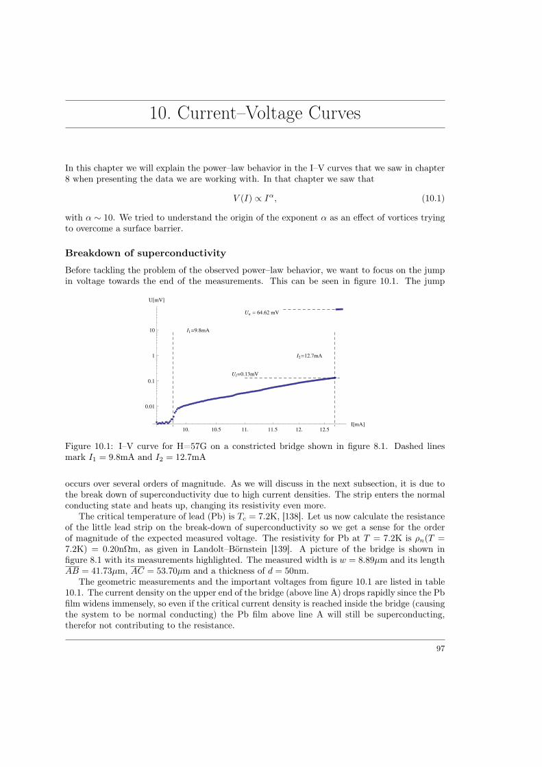
10. Current–Voltage Curves

In this chapter we will explain the power–law behavior in the I–V curves that we saw in chapter8 when presenting the data we are working with. In that chapter we saw that

V (I) ∝ Iα, (10.1)

with α ∼ 10. We tried to understand the origin of the exponent α as an effect of vortices tryingto overcome a surface barrier.

Breakdown of superconductivity

Before tackling the problem of the observed power–law behavior, we want to focus on the jumpin voltage towards the end of the measurements. This can be seen in figure 10.1. The jump

10. 10.5 11. 11.5 12. 12.5I@mAD

0.01

0.1

1

10

U@mVDUu = 64.62 mV

Ul=0.13mV

I1=9.8mA

I2=12.7mA

Figure 10.1: I–V curve for H=57G on a constricted bridge shown in figure 8.1. Dashed linesmark I1 = 9.8mA and I2 = 12.7mA

occurs over several orders of magnitude. As we will discuss in the next subsection, it is due tothe break down of superconductivity due to high current densities. The strip enters the normalconducting state and heats up, changing its resistivity even more.

The critical temperature of lead (Pb) is Tc = 7.2K, [138]. Let us now calculate the resistanceof the little lead strip on the break-down of superconductivity so we get a sense for the orderof magnitude of the expected measured voltage. The resistivity for Pb at T = 7.2K is ρn(T =7.2K) = 0.20nΩm, as given in Landolt–Börnstein [139]. A picture of the bridge is shown infigure 8.1 with its measurements highlighted. The measured width is w = 8.89µm and its lengthAB = 41.73µm, AC = 53.70µm and a thickness of d = 50nm.

The geometric measurements and the important voltages from figure 10.1 are listed in table10.1. The current density on the upper end of the bridge (above line A) drops rapidly since the Pbfilm widens immensely, so even if the critical current density is reached inside the bridge (causingthe system to be normal conducting) the Pb film above line A will still be superconducting,therefor not contributing to the resistance.

97

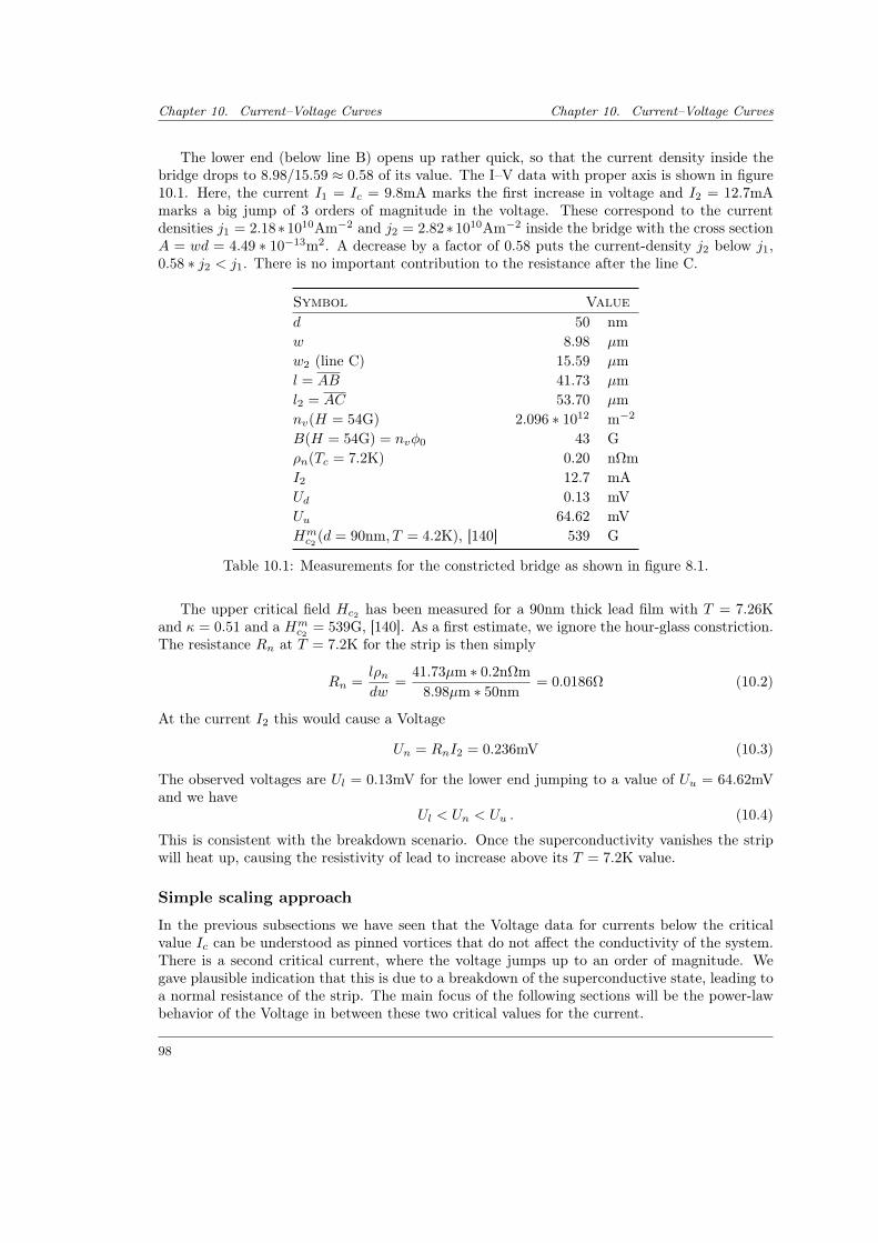
Chapter 10. Current–Voltage Curves Chapter 10. Current–Voltage Curves

The lower end (below line B) opens up rather quick, so that the current density inside thebridge drops to 8.98/15.59 ≈ 0.58 of its value. The I–V data with proper axis is shown in figure10.1. Here, the current I1 = Ic = 9.8mA marks the first increase in voltage and I2 = 12.7mAmarks a big jump of 3 orders of magnitude in the voltage. These correspond to the currentdensities j1 = 2.18∗1010Am−2 and j2 = 2.82∗1010Am−2 inside the bridge with the cross sectionA = wd = 4.49 ∗ 10−13m2. A decrease by a factor of 0.58 puts the current-density j2 below j1,0.58 ∗ j2 < j1. There is no important contribution to the resistance after the line C.

Symbol Valued 50 nmw 8.98 µmw2 (line C) 15.59 µml = AB 41.73 µml2 = AC 53.70 µmnv(H = 54G) 2.096 ∗ 1012 m−2

B(H = 54G) = nvφ0 43 Gρn(Tc = 7.2K) 0.20 nΩmI2 12.7 mAUd 0.13 mVUu 64.62 mVHmc2 (d = 90nm, T = 4.2K), [140] 539 G

Table 10.1: Measurements for the constricted bridge as shown in figure 8.1.

The upper critical field Hc2 has been measured for a 90nm thick lead film with T = 7.26Kand κ = 0.51 and a Hm

c2 = 539G, [140]. As a first estimate, we ignore the hour-glass constriction.The resistance Rn at T = 7.2K for the strip is then simply

Rn =lρndw

=41.73µm ∗ 0.2nΩm

8.98µm ∗ 50nm= 0.0186Ω (10.2)

At the current I2 this would cause a Voltage

Un = RnI2 = 0.236mV (10.3)

The observed voltages are Ul = 0.13mV for the lower end jumping to a value of Uu = 64.62mVand we have

Ul < Un < Uu . (10.4)

This is consistent with the breakdown scenario. Once the superconductivity vanishes the stripwill heat up, causing the resistivity of lead to increase above its T = 7.2K value.

Simple scaling approach

In the previous subsections we have seen that the Voltage data for currents below the criticalvalue Ic can be understood as pinned vortices that do not affect the conductivity of the system.There is a second critical current, where the voltage jumps up to an order of magnitude. Wegave plausible indication that this is due to a breakdown of the superconductive state, leading toa normal resistance of the strip. The main focus of the following sections will be the power-lawbehavior of the Voltage in between these two critical values for the current.

98

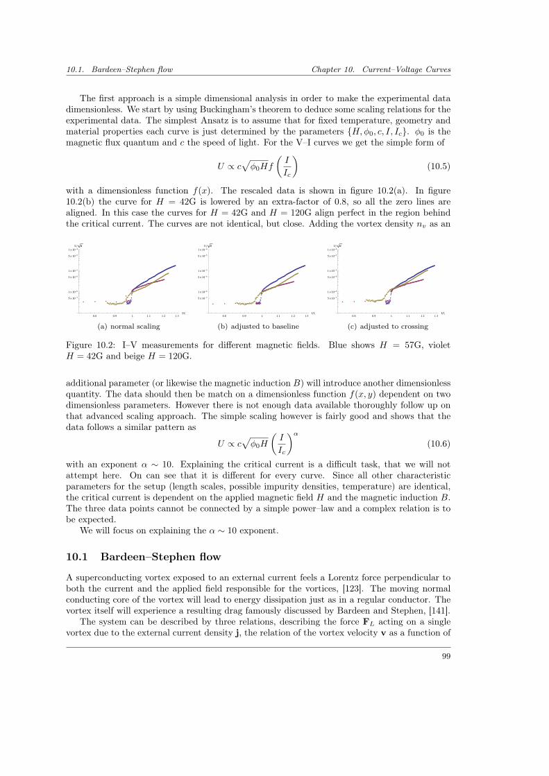
10.1. Bardeen–Stephen flow Chapter 10. Current–Voltage Curves

The first approach is a simple dimensional analysis in order to make the experimental datadimensionless. We start by using Buckingham’s theorem to deduce some scaling relations for theexperimental data. The simplest Ansatz is to assume that for fixed temperature, geometry andmaterial properties each curve is just determined by the parameters H,φ0, c, I, Ic. φ0 is themagnetic flux quantum and c the speed of light. For the V–I curves we get the simple form of

U ∝ c√φ0Hf

(I

Ic

)(10.5)

with a dimensionless function f(x). The rescaled data is shown in figure 10.2(a). In figure10.2(b) the curve for H = 42G is lowered by an extra-factor of 0.8, so all the zero lines arealigned. In this case the curves for H = 42G and H = 120G align perfect in the region behindthe critical current. The curves are not identical, but close. Adding the vortex density nv as an

0.8 0.9 1. 1.1 1.2 1.3IIc

5 ´ 10-7

1 ´ 10-6

5 ´ 10-6

1 ´ 10-5

5 ´ 10-5

1 ´ 10-4

U B

(a) normal scaling

0.8 0.9 1. 1.1 1.2 1.3IIc

5 ´ 10-7

1 ´ 10-6

5 ´ 10-6

1 ´ 10-5

5 ´ 10-5

1 ´ 10-4

U B

(b) adjusted to baseline

0.8 0.9 1. 1.1 1.2 1.3IIc

5 ´ 10-7

1 ´ 10-6

5 ´ 10-6

1 ´ 10-5

5 ´ 10-5

1 ´ 10-4

U B

(c) adjusted to crossing

Figure 10.2: I–V measurements for different magnetic fields. Blue shows H = 57G, violetH = 42G and beige H = 120G.

additional parameter (or likewise the magnetic induction B) will introduce another dimensionlessquantity. The data should then be match on a dimensionless function f(x, y) dependent on twodimensionless parameters. However there is not enough data available thoroughly follow up onthat advanced scaling approach. The simple scaling however is fairly good and shows that thedata follows a similar pattern as

U ∝ c√φ0H

(I

Ic

)α(10.6)

with an exponent α ∼ 10. Explaining the critical current is a difficult task, that we will notattempt here. On can see that it is different for every curve. Since all other characteristicparameters for the setup (length scales, possible impurity densities, temperature) are identical,the critical current is dependent on the applied magnetic field H and the magnetic induction B.The three data points cannot be connected by a simple power–law and a complex relation is tobe expected.

We will focus on explaining the α ∼ 10 exponent.

10.1 Bardeen–Stephen flow

A superconducting vortex exposed to an external current feels a Lorentz force perpendicular toboth the current and the applied field responsible for the vortices, [123]. The moving normalconducting core of the vortex will lead to energy dissipation just as in a regular conductor. Thevortex itself will experience a resulting drag famously discussed by Bardeen and Stephen, [141].

The system can be described by three relations, describing the force FL acting on a singlevortex due to the external current density j, the relation of the vortex velocity v as a function of

99

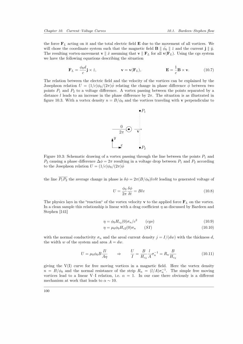
Chapter 10. Current–Voltage Curves 10.1. Bardeen–Stephen flow

the force FL acting on it and the total electric field E due to the movement of all vortices. Wewill chose the coordinate system such that the magnetic field B ‖ φ0 ‖ z and the current j ‖ y.The resulting vortex-movement v ‖ x assuming that v ‖ FL for all v(FL). Using the cgs systemwe have the following equations describing the situation

FL =φ0d

cj× z, v = v(FL), E =

1

cB× v. (10.7)

The relation between the electric field and the velocity of the vortices can be explained by theJosephson relation U = (1/c)φ0/(2π)φ relating the change in phase difference φ between twopoints P1 and P2 to a voltage difference. A vortex passing between the points separated by adistance l leads to an increase in the phase difference by 2π. The situation is as illustrated infigure 10.3. With a vortex density n = B/φ0 and the vortices traveling with v perpendicular to

y

x

P1

P2

02π v

Figure 10.3: Schematic drawing of a vortex passing through the line between the points P1 andP2 causing a phase difference ∆φ = 2π resulting in a voltage drop between P1 and P2 accordingto the Josephson relation U = (1/c)φ0/(2π)φ

the line P1P2 the average change in phase is δφ = 2π(B/φ0)lvδt leading to generated voltage of

U =φ0

2π

δφ

δt= Blv (10.8)

The physics lays in the “reaction“ of the vortex velocity v to the applied force FL on the vortex.In a clean sample this relationship is linear with a drag coefficient η as discussed by Bardeen andStephen [141]

η = φ0Hc2(0)σn/c2 (cgs) (10.9)

η = µ0φ0Hc2(0)σn (SI) (10.10)

with the normal conductivity σn and the areal current density j = I/(dw) with the thickness d,the width w of the system and area A = dw.

U = µ0φ0BIl

Aη⇒ U

I=

B

Hc2

l

Aσ−1n = Rn

B

Hc2

(10.11)

giving the V(I) curve for free moving vortices in a magnetic field. Here the vortex densityn = B/φ0 and the normal resistance of the strip Rn = (l/A)σ−1

n . The simple free movingvortices lead to a linear V–I relation, i.e. α = 1. In our case there obviously is a differentmechanism at work that leads to α ∼ 10.

100

10.2. Surface barrier Chapter 10. Current–Voltage Curves

10.2 Surface barrier

We saw that simple free moving vortices lead to a linear relation between the measured voltageand the applied current, i.e. α = 1. This theory however only looks at free moving vortices insidethe sample. In the present experimental setup we are dealing with a small strip that has anhour–glass constriction. One effect that can produce the observed power–law behavior is due tovortices interacting with the boundary of the strip.

This type of surface barrier is known in the literature as the Bean–Livingston barrier, [142,143]. The simple picture is the following. Close to the boundary of the strip the vortex will feelits mirror image or antivortex, similar to the mirror charges in electrostatic. There is no currentflowing through the boundary, meaning that the normal component of the current density onthe boundary vanishes. A condition that is satisfied by the vortex–antivortex pair construction.The applied current will try to push the vortex away from the boundary inside the sample. Theantivortex counteracts and will push the vortex towards the boundary. The resulting potentialbarrier or activation energy EA can be overcome by thermal fluctuations. Since the interactionbetween the vortex and its mirror image is logarithmic on short scales and the activation rate Rbeing of Arrehnius form

R ∝ exp

[− EAkbT

](10.12)

this will produce a power–law behavior for the resulting voltage. In this section, we will examinethe resulting voltage response due to vortices entering the sample.

The vortex–vortex interaction for Pearl vortices has been calculated by Pearl [125] to be

V (r′) =φ2

0

2Λµ0

[H0

( rΛ

)− Y0

( rΛ

)](10.13)

in SI units with the Struve function Hn and the modified Bessel function of the second kind Yn.Λ = 2λ2/d is the effective penetration depth. The interaction force has the form

F12(r′) = − φ20

2Λ2µ0

[H1

(r′

Λ

)− Y1

(r′

Λ

)− 2

π

]. (10.14)

The potential can be expanded around the limiting cases for r Λ and r Λ, as shown in[144].

V (r) =

φ2

0

πµ0Λ ln(1.135Λ

r

): r

Λ 1φ2

0

µ0πr: r

Λ 1

They can be combined into an interpolation formula

V (r) ≈ φ20

πµ0Λln

(1.135

Λ

r− 0.135Λ

4.5Λ + r+ 1

). (10.15)

as shown by Brandt, [144]. Note that the equation used by Brandt use a definition of thepenetration length Λ without the factor of 2. The interpolation formula is very accurate and isused since it is easier to handle than the Struve and Bessel function. For later convenience, wewill introduce the characteristic energy scale of the interaction

E0 =φ2

0

πµ0Λ(10.16)

As the coordinate system, we will choose the applied magnetic field perpendicular to the stripin the z-direction and the current moving in the y-direction as shown in figure 10.4. The Lorentz

101

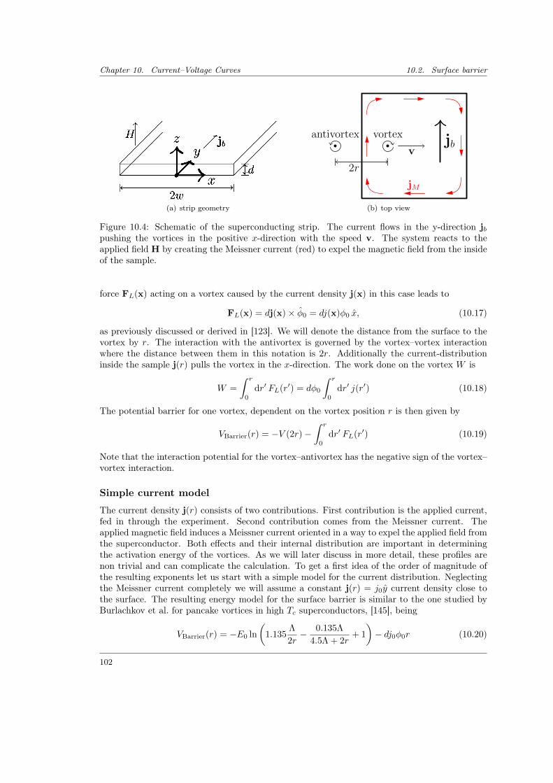
Chapter 10. Current–Voltage Curves 10.2. Surface barrier

(a) strip geometry

jb

jM

vortexantivortex

2r

v

(b) top view

Figure 10.4: Schematic of the superconducting strip. The current flows in the y-direction jbpushing the vortices in the positive x-direction with the speed v. The system reacts to theapplied field H by creating the Meissner current (red) to expel the magnetic field from the insideof the sample.

force FL(x) acting on a vortex caused by the current density j(x) in this case leads to

FL(x) = dj(x)× φ0 = dj(x)φ0 x, (10.17)

as previously discussed or derived in [123]. We will denote the distance from the surface to thevortex by r. The interaction with the antivortex is governed by the vortex–vortex interactionwhere the distance between them in this notation is 2r. Additionally the current-distributioninside the sample j(r) pulls the vortex in the x-direction. The work done on the vortex W is

W =

∫ r

0

dr′ FL(r′) = dφ0

∫ r

0

dr′ j(r′) (10.18)

The potential barrier for one vortex, dependent on the vortex position r is then given by

VBarrier(r) = −V (2r)−∫ r

0

dr′ FL(r′) (10.19)

Note that the interaction potential for the vortex–antivortex has the negative sign of the vortex–vortex interaction.

Simple current model

The current density j(r) consists of two contributions. First contribution is the applied current,fed in through the experiment. Second contribution comes from the Meissner current. Theapplied magnetic field induces a Meissner current oriented in a way to expel the applied field fromthe superconductor. Both effects and their internal distribution are important in determiningthe activation energy of the vortices. As we will later discuss in more detail, these profiles arenon trivial and can complicate the calculation. To get a first idea of the order of magnitude ofthe resulting exponents let us start with a simple model for the current distribution. Neglectingthe Meissner current completely we will assume a constant j(r) = j0y current density close tothe surface. The resulting energy model for the surface barrier is similar to the one studied byBurlachkov et al. for pancake vortices in high Tc superconductors, [145], being

VBarrier(r) = −E0 ln

(1.135

Λ

2r− 0.135Λ

4.5Λ + 2r+ 1

)− dj0φ0r (10.20)

102

10.2. Surface barrier Chapter 10. Current–Voltage Curves

The difference lies in the interaction strength of the logarithmic term, since we are dealing withPearl vortices in this scenario. The current density flowing through the sample is assumed to beconstant for the time being, identical to the profile used by Burlachkov et al. Later we will usea more realistic current profile for the thin films.

Looking at the interaction profile, we see that the stronger the applied current, the smallerthe distance needed to achieve enough energy to separate the vortex from its mirror image.The equilibrium distance r0 will therefore be smaller for higher applied current densities j0.Assuming a strong enough current, so that the separation process will happen close to thesurface, i.e. r0 ∼ O(Λ) the surface barrier can be simplified to

VBarrier(r) ≈ −E0 ln

(1.135

Λ

2r

)− dj0φ0r (10.21)

The maximum of the potential is reached at the equilibrium distance r0 of

r0 =E0

dj0φ0(10.22)

leading to an activation energy

EA = E0 ln

(2E0

1.135Λ dj0φ0

)− E0 (10.23)

The Arrehnius type penetration rate R is then proportional to

R ∝ exp

[− EAkbT

]= eE0

(1.135Λdj0φ0

2E0

) E0kbT

∝ Iα (10.24)

with the exponent

α =E0

kbT(10.25)

Plugging in the values for Λ in our system we get

E0 =φ2

0

µ0πΛ=

2.4× 105K : Λ = 330nm4.6× 105K : Λ = 170nm

The resulting exponent for the current dependency for temperatures around T = 4.2K is

α ∼ 105 (10.26)

several orders of magnitude larger than the observed α ≈ 10. To obtain an exponent of theobserved magnitude the temperature would have to exceed the bulk melting temperature T ≈600K of Pb by orders of magnitude. For the material value see table E.1. The expected heatingeffects close to the second jump in voltage, as seen in figure 10.1 and discussed in the previoussections, will not change the discrepancy in the exponents. The large exponent is similar to theone for the theory of thermal activated flux creep as discussed in literature, [143, 145–147].

Current distribution inside the strip

In the previous part, we used a constant current profile, mainly for its simplicity. Let us nowfocus more on the actual current distribution inside the thin strip. In the absence of vortices andan applied current, only the Meissner current is present. We consider the strip thickness d to

103

Chapter 10. Current–Voltage Curves 10.2. Surface barrier

be small enough so that the current distribution along the z-axis can be treated as homogenous.For a strip of width 2w going from −w to w in the x-direction. The current profile is known tobe

jM (x) = − 2H x

d√w2 − x2

(10.27)

as can be found in e.g. [148–156]. The current profile exhibits a characteristic square-root di-vergence towards the surface of the film, when x → ±w. In the presents of vortices, magneticflux was able to penetrate into the thin film. Averaged over scales larger than the vortex size,this leads to the magnetic induction B inside the sample. The Meissner current now only has tocompensate the reduced field H ′ = H −B/µ0.

The total transport current I flowing through the strip is distributed as

jT (x) =I

πd√w2 − x2

(10.28)

also discussed in [148]. The work W done by the current moving the vortex by the distance raway from the outer border at −w is written as

W = dφ0

∫ −w+r

−wdr′(jM (r′) + jT (r′)) (10.29)

As discussed earlier, the surface barrier is now written as

VBarrier(r) = −V (2r)−W (10.30)

In the case of strong enough currents, the equilibrium position r0 will be small, i.e. of the orderO(Λ) and the interaction potential can be simplified as V (2r) ≈ E0 ln

(1.135 Λ

2r

). The condition

for the equilibrium position ∂rVBarrier(r)|r0 = 0 results in the equation

E0

r0=

2H ′(w − r0)√r(2w − r0)

+I

π√r(2w − r0)

. (10.31)

Expanding the right hand side of the equation for small r0 we obtain

E0

r0≈ φ0

(I

π√

2w+√

2wH ′)

1√r0, (10.32)

with the equilibrium distance

r0 ≈(

E0

φ0I

π√

2w+√

2wH ′ φ0

)2

. (10.33)

The activation energy then works out to be

EA = E0 ln

(2r0

1.135Λ

)− φ0I − 2φ0H

′√r0(2w − r0) + φ0I arccos

(r0

w− 1). (10.34)

The applied total currents are of the order of ∼ 10mA. The energy of the current is of the sameorder as E0 with

φ0I ∼ 1.5 · 105K. (10.35)

104

10.2. Surface barrier Chapter 10. Current–Voltage Curves

For small equilibrium positions r0, we can expand the expression for EA as

EA = E0 ln

(2r0

1.135Λ

)− 2φ0H

′√2wr0 −φ0I√r0

π√w

, (10.36)

leading to the simple form of

EA = E0 ln

(2r0

1.135Λ

)− 2E0. (10.37)

The penetration rate then yields

R ∝ exp

[− EAkbT

]= e

2E0kbT

(1.135Λ

2r0

) E0kbT

∝(

1.135Λ

2E20

(φ0I

π√

2w+√

2wH ′ φ0

)2) E0kbT

(10.38)

Interestingly enough the exponent ∝ Iα in this case is larger by a factor of 2 compared to theconstant current assumption

α = 2E0

kbT(10.39)

The geometry of the setup makes the system even more sensitive to the current, which leads toa higher exponent α. A more accurate description of the current distribution actually increasesthe exponent. Additionally including geometric effects from the hour–glass construction will notreduce the exponent.

Possible screening of vortex–vortex interaction

The thermally activated entering of the vortices into the strip is able to produce a power–law response of the voltage to the applied current. However the theory predicts an exponentα = 2E0/kbT that is several orders of magnitude higher then the observed value of α ∼ 10. Aprocess that can reduce the interaction strength E0 would reduce the exponent. Screening effectsdue to spontaneously created vortex–antivortex pairs could be one possible mechanism to reduceE0. Thermally created pairs would screen the interaction, similar to the RG for the Coulomb–gaspicture of the XY model, [10]. However there are two problems with this approach. Screeningeffects take place on large scales. On short distances r ∼ Λ the effects will be slim. Second, theenergy cost to create a pair compared to the thermal energy is too large to be possible.

The core energy of a vortex has been calculated by Pearl, and according to [126, 157] is

Ev = E0

[ln

(Λ

rc

)+

1

24

(rcξ

)2]

(10.40)

with E0 being the energy-scale of the interaction, the size of the vortex core rc and the correlationlength ξ. We already computed the interaction strength to be

E0 =φ2

0

µ0πΛ=

2.4× 105K : Λ = 330nm4.6× 105K : Λ = 170nm

Taking the vortex–size to be of the order of the correlation length ξ, we get a pre-factor

Ev = E0 ×

1.93 : Λ = 330nm1.27 : Λ = 170nm

105

Chapter 10. Current–Voltage Curves 10.3. Discussion

Making the core energy several orders of magnitude larger than the thermal energy T = 4.2K.Screening effects due to thermal activated vortex–antivortex pairs is therefor impossible.

10.3 Discussion

In this chapter we have looked into the conductivity measurements done on the constrictedbridge setup. The characteristic curve as shown in figure 10.1 features 3 distinct scenarios. Forlow currents we have no measurable voltage. The strip is still in the superconducting phase atT = 4.2K < Tc = 7.2K and vortices are pinned, as seen in figure 8.4(a). After the vortices aredepinned , a power–law behavior in the voltage of the form

U ∝ Iα (10.41)

was observed, with an exponent of α ∼ 10. This was followed by a jump in the voltage thatwe could trace back to a thermal quench in the system, where the strip was becoming normalconducting again.

The main focus lay in finding an explanation for the power-law behavior with the exponentα ∼ 10. We saw that thermal activated vortices surmounting a surface barrier will lead to apower–law behavior. However the predicted exponent α ∼ 105 for this theory was several ordersof magnitude larger than the observed one. Even including the internal distribution of the currentinside the thin strip did not change the discrepancy. Quite the opposite. The internal currentdistribution makes the system more sensitive to the current then a simple constant distribution.The resulting exponent is even larger by a factor of 2.

The energy scale of the current φ0I ∼ E0 is of the same order as the vortex interactionstrength and core energy of the vortices. The next step would have been to look more detailedinto the effect of possible pair creation inside the sample due to the current and its effect onthe V–I curves. The geometry and local impurities in the surface itself can also reduce thesurface barrier and change the power-law behavior compared to the simple model used so far.At this point however, the collaboration was focusing mainly on the vortex dynamics and westopped exploring additional modifications to the surface barrier model. The data on the voltagemeasurements were too thin to extract more qualitative features other than the relative largeexponent α ∼ 10. The experimental setup in general was geared towards the vortex dynamics.Especially the hour–glass constriction in the strips complicates the voltage curve analysis. Thesurface barrier model successfully explains the power–law, but due to time constraints we werenot able to identify the missing contributions that produce the right order of magnitude for theexponent α.

106

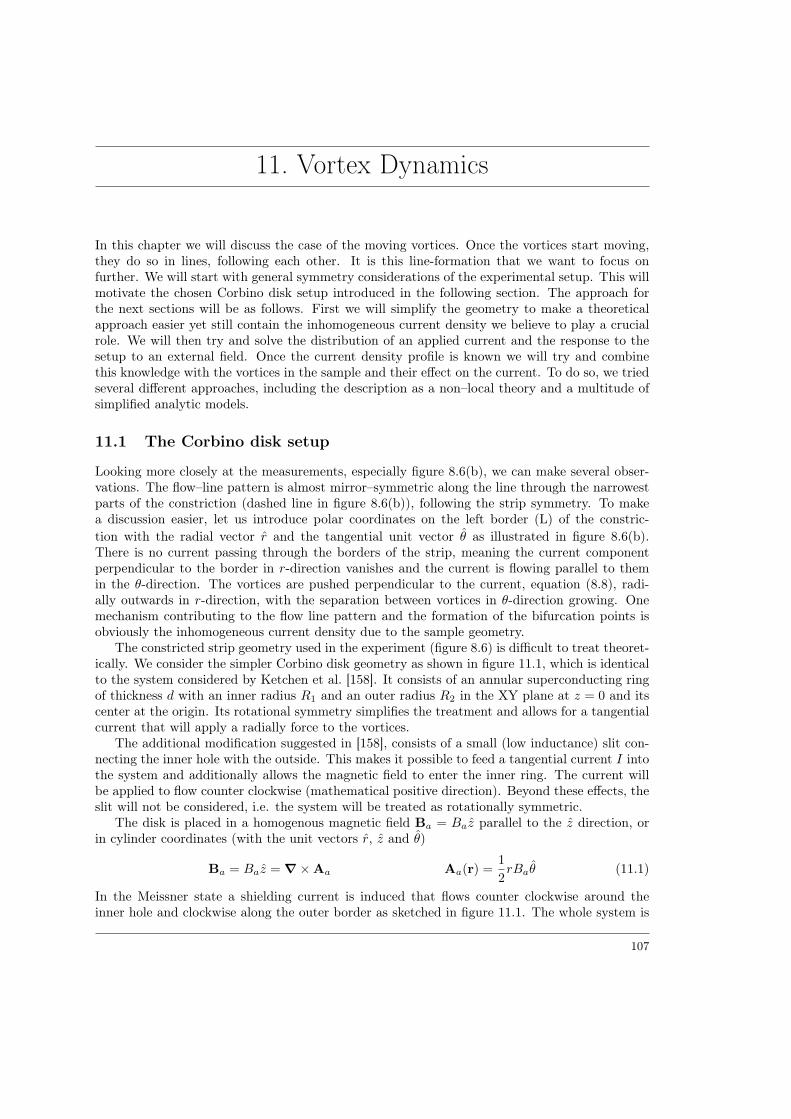
11. Vortex Dynamics

In this chapter we will discuss the case of the moving vortices. Once the vortices start moving,they do so in lines, following each other. It is this line-formation that we want to focus onfurther. We will start with general symmetry considerations of the experimental setup. This willmotivate the chosen Corbino disk setup introduced in the following section. The approach forthe next sections will be as follows. First we will simplify the geometry to make a theoreticalapproach easier yet still contain the inhomogeneous current density we believe to play a crucialrole. We will then try and solve the distribution of an applied current and the response to thesetup to an external field. Once the current density profile is known we will try and combinethis knowledge with the vortices in the sample and their effect on the current. To do so, we triedseveral different approaches, including the description as a non–local theory and a multitude ofsimplified analytic models.

11.1 The Corbino disk setup

Looking more closely at the measurements, especially figure 8.6(b), we can make several obser-vations. The flow–line pattern is almost mirror–symmetric along the line through the narrowestparts of the constriction (dashed line in figure 8.6(b)), following the strip symmetry. To makea discussion easier, let us introduce polar coordinates on the left border (L) of the constric-tion with the radial vector r and the tangential unit vector θ as illustrated in figure 8.6(b).There is no current passing through the borders of the strip, meaning the current componentperpendicular to the border in r-direction vanishes and the current is flowing parallel to themin the θ-direction. The vortices are pushed perpendicular to the current, equation (8.8), radi-ally outwards in r-direction, with the separation between vortices in θ-direction growing. Onemechanism contributing to the flow line pattern and the formation of the bifurcation points isobviously the inhomogeneous current density due to the sample geometry.

The constricted strip geometry used in the experiment (figure 8.6) is difficult to treat theoret-ically. We consider the simpler Corbino disk geometry as shown in figure 11.1, which is identicalto the system considered by Ketchen et al. [158]. It consists of an annular superconducting ringof thickness d with an inner radius R1 and an outer radius R2 in the XY plane at z = 0 and itscenter at the origin. Its rotational symmetry simplifies the treatment and allows for a tangentialcurrent that will apply a radially force to the vortices.

The additional modification suggested in [158], consists of a small (low inductance) slit con-necting the inner hole with the outside. This makes it possible to feed a tangential current I intothe system and additionally allows the magnetic field to enter the inner ring. The current willbe applied to flow counter clockwise (mathematical positive direction). Beyond these effects, theslit will not be considered, i.e. the system will be treated as rotationally symmetric.

The disk is placed in a homogenous magnetic field Ba = Baz parallel to the z direction, orin cylinder coordinates (with the unit vectors r, z and θ)

Ba = Baz = ∇×Aa Aa(r) =1

2rBaθ (11.1)

In the Meissner state a shielding current is induced that flows counter clockwise around theinner hole and clockwise along the outer border as sketched in figure 11.1. The whole system is

107

Chapter 11. Vortex Dynamics 11.1. The Corbino disk setup

Figure 11.1: Corbino disk configurationas considered in our calculations. The fig-ure is taken from [158]. In our notationthe inner radius is labeled with R1 whilethe outer radius is R2. The disk lies inthe XY plane at z = 0 with an appliedmagnetic field Ba = Baz parallel to the zdirection. The small slit allows the mag-netic field to enter the hole and makesit possible to feed in an external tangen-tial current I into the system. The direc-tion of the shielding current induced bythe magnetic field in the Meissner stateis sketched by the black arrows.

rotationally symmetric and the resultingB of the system has no θ component nor a θ-dependency.This means we can write the magnetic field of the system B as

B(r) = Br(r, z)r +Bz(r, z)z (11.2)

which is satisfied by the following ansatz for the vector potential

A(r) = Aθ(r, z)θ. (11.3)

In the limits far away from the sample, the field is equal to the applied field, which makes itconvenient to introduce the reduced vector potential f(r, z) as

Aθ(r, z) = f(r, z) +1

2rBa (11.4)

with the condition that f(r, z) vanishes far away from the sample, i.e.

limz→±∞

f(r, z) = 0, limr→∞

f(r, z) = 0. (11.5)

This reduces the whole discussion of the system to the determination of the vector potentialf(r, z), which is connected to the current distribution via the Maxwell equation

∇×B =4π

cj(r). (11.6)

The current density j(r) of the system is made to flow counter clockwise and consists only ofa tangential component in θ-direction. Approximating the film by a δ(z)-thin sheet, it can bewritten as

j(r, z) = j(r)δ(z)θ. (11.7)The system itself is described by the Maxwell and London equations discussed in the previouschapter 9. This leads to a differential equation for the reduced vector potential f(r, z)[

∂2

∂z2+

∂

∂r

1

r

∂

∂rr

]f(r, z) = −4π

cj(r)δ(z) =

2Λδ(z)

[f(r, z) + Bar

2 −nφ0

2πr

], R1 ≤ r ≤ R2,

0 , elsewhere.(11.8)

A detailed derivation of this equation is shown in appendix F.2.

108

11.2. The current distribution in the Corbino disk Chapter 11. Vortex Dynamics

11.2 The current distribution in the Corbino disk

The current density j(r) is determined by the differential equation (11.8). Due to its linearnature, we can treat the inhomogeneous terms separately. Imagine the scenario where there isno applied field, Ba = 0, but a current I 6= 0 in the disk. The current circling the hole producesa net magnetic field inside it, which is identical to a trapped flux. Vice versa, a trapped fluxinside the Corbino disk is accompanied with a current profile j(r) around it and therefor a finitecurrent I. We see that the two are equivalent and we can think of the current I fed into thesystem as a trapped flux φf = nφ0 inside the ring. The other scenario we consider is an appliedfield Ba 6= 0 without a current, I = 0. Here, the superconducting disk, in its Meissner phase,tries to expel the magnetic field inducing a shielding current that flows around the outsides of thedisk as shown in figure 11.1. No net current is present and no flux is trapped in the inner ring.The full current j(r) then splits into the two contribution jφ(r) and jB(r). The current jφ(r)is due to the trapped flux φf in the hole of the disk and the current jB(r) due to the magneticfield without a trapped flux. The relation of the densities to the total current I is given as

I =

∫ R2

R1

dr j(r), j(r) = jφ(r) + jB(r). (11.9)

It is easier to discuss the effects separately.There are several known analytic results. One is the the case of a superconducting sheet with

a hole (R2 →∞) in the perfect diamagnetic state, i.e. Λ = 0. Here, the current density jφ(r) isgiven as

jφ(r) =φfc

4π2

1

r√r2 −R2

1

Θ(r −R1) (11.10)

and as has been calculated by Ketchen et. al. [158] by mapping to an electrostatic problem. Thesecond known case is that of a perfect diamagnetic disk in a magnetic field, [158], giving us

jB(r) = −Bacπ2

r√R2

2 − r2Θ(R2 − r). (11.11)

Lastly, we have the famous result by Pearl, which is equivalent to a trapped flux in a thin film(R1 → 0 and R2 →∞) that results in the current density jP (r) for the Pearl vortex as

jP (r) =φ0c

8πΛ2

[H1

( rΛ

)− Y1

( rΛ

)− 2

π

]≈ φfc

4π2

1

r(r + Λ), (11.12)

which can be found in [137]. Here Hn(x) is the Struve function and Yn(x) the modified Besselfunction. In appendix F.3 we show that all these known limiting cases are indeed analyticsolutions to the differential equation (11.8). We do this by transforming the differential equationto an integral equation which can then be solved in aforementioned limits, see appendix F.2.

On the basis of the integral equations and the known limiting cases, we can construct anapproximate profile of the current density. A more detailed discussion of the literature and theknown approximate profiles is done in appendix F.1. The first approximate profile is with a setof free parameters c0, c1, c2 can be written down as

jφ(r) =φfc

4π2

c0 + c1rR2

+ c2r2

R22

r√

(r +R1 + Λ)(r −R1 + Λ)√

(1− rR2

+ ΛR2

)(1 + rR2

+ ΛR2

)Θ(r −R1) Θ(R2 − r).

(11.13)

109

Chapter 11. Vortex Dynamics 11.3. Non–local theory

It satisfies the known limiting cases. Computing

limR1→0

limR2→∞

jφ(r) =φfc

4π2

c0r(r + Λ)

(11.14)

we see that it turns into the approximate Pearl solution for c1 = 1 and for

limΛ→0

limR2→∞

jφ(r) =φfc

4π2

c0

r√r2 −R2

1

(11.15)

the solution becomes becomes exact for c0 = 1. The approximate current profile for the responseto an magnetic field uses the free parameters d0, d1, d2, d4 and is given by

jB(r) = −Bac4π

R2

(d0 + d1

rR2

+ d2r2

R22

+ d4r4

R42

)√

(r +R1 + Λ)(r −R1 + Λ)√

(1− rR2

+ ΛR2

)(1 + rR2

+ ΛR2

)Θ(r −R1) Θ(R2 − r).

(11.16)Computing again the the limiting case to verify that it indeed satisfies the known limiting con-ditions, we get

limΛ→0

limR1→0

jB(r) = −Bac4π

R22

(d0 + d1

rR2

+ d2r2

R22

+ d4r4

R42

)r√R2

2 − r2. (11.17)

This is the exact solution of the problem for d0 = d1 = d4 = 0 and d2 = 1. The numericalprocedure we use to determine the coefficients c0, c1, c2 and d0, d1, d2, d4 is discussed atlength in appendix F.4. Once the coefficients are determined, the condition for the total currentin the system from equation (11.9) will be used to fix φf .

11.3 Non–local theory

Now that we have a very accurate model of the current distribution inside the disk, the nexttask is adding the superconducting vortices. On approach we followed is illustrated in thissection. Outside the disk we are only dealing with free fields. The idea here is to take the full3D Maxwell equation for the magnetic field and integrate out the part outside the disk. Thiswill create a purely 2D theory with the trade off being non-local interactions in the fields. Thecalculation follows the procedure in reducing the dimensionality of the Hamiltonian as outlinedby Radzihovsky, [159]. The hope is to use this 2D theory and use it as a more convenient jumpoff point in connecting the current distribution to the penetrating vortices.

Starting from a free-field system, we want to integrate out all the bulk degrees of freedom toobtain an effective system only with degrees of freedom in the z = 0 plane. Ignoring dynamicaleffects A = 0 the Hamiltonian reduces to

H =1

8π

∫d3x (B−Ba)2 (11.18)

in cgs units. Introducing the vector potential A as

B = ∇×A (11.19)

in order to write the theory simpler terms. Starting with the case of no applied field Ba = 0, weare dealing with the simplified theory

H =1

8π

∫d3x (∇×A)2 . (11.20)

110

11.3. Non–local theory Chapter 11. Vortex Dynamics

In order to perform the partial integration we need the following two identities

(∇×A)2 = (εijk∂jAkei)(εlmn∂mAnel) = εijkεimn(∂jAk)(∂mAn)

(∇×∇×A)A = (∇×∇×A)nAn = εnmi∂m(∇×A)iAn = −εijkεimn(∂m∂jAk)An

We can see that the two expressions can be made identical by partial integration. The theoryfor the free field can then be written as

H =1

8π

∫d3x (∇×A)2 =

1

8π

∫d3x (∇×∇×A)A = − 1

8π

∫d3x (∇2A)A (11.21)

where we have used the Coulomb gauge ∇A = 0. Now we want to Fourier transform the systemand afterward integrate out all degrees of freedom outside the z = 0 plane, leaving an effective2D system. For this we want to introduce the following notation

x = (r, z) q = (k, ω) Ap(r) = A(r, z = 0) (11.22)

where x and q are related via the Fourier transform. The final system should only be r dependentand is described by the 2D plane vector potential Ap(r). The Fourier transformed Hamiltonianreads as

βH =β

8π

∫d3q

(2π)3q2AqA−q (11.23)

=1

2

∫q

∫q′AqG(q,q′)Aq′ (11.24)

G(q,q′) =β

4π

1

(2π)3q2δ(q + q′) (11.25)

Here the integral notation∫q

=∫

d3q has been used. We already included the factor β = 1/kbT ,since we will be using βH in the partition function Z of the system.

Z =

∫D[A]e−βH (11.26)

Introducing the degrees of freedom in the z = 0 plane, Ap, via a delta distribution

Z =

∫D[A]

∫D[Ap]δ(A(r, z = 0)−Ap(r))e−βH =

∫D[Ap]e

−βHp (11.27)

e−βHp =

∫D[A]δ(A(r, z = 0)−Ap(r))e−βH (11.28)

we can obtain our boundary Hamiltonian Hp. It will be living only in the z = 0 plane, once theintegration over

∫D[A] is performed . This can be evaluated by using the Fourier representation

of the δ-distribution for the Fourier components of the degrees of freedom.

Ap(r)→ Ap(k) (11.29)A(x)→ Aq (11.30)

A(r, z = 0)→∫

dω

2πAq (11.31)

δ(Ap −A(r, z = 0))→∫D[λk]eı

∫kλk(Ap(k)−

∫dω2πAq) (11.32)

111

Chapter 11. Vortex Dynamics 11.3. Non–local theory

For the Boundary Hamiltonian we get the following relations based on the partition function

e−βHp =

∫D[A]

∫D[λk] exp

[−1

2

∫q

∫q′AqG(q,q′)Aq′ − ı

∫q

λk2π

Aq + ı

∫k

λkAp(k)

](11.33)

Here we can perform the integration over the Aq components, since they form a quadratic theory.

e−βHp =

∫D[λk] exp

[−1

2

∫q

∫q′λk

1

(2π)2G−1(q,q′)λk′ + ı

∫k

λkAp(k)

](11.34)

The inverse of G can be calculated to be

G−1(q,q′) =1

β4π(2π)3 1

q2δ(q− q′) (11.35)

The new fields and therefore λk are not dependent on z (and equivalently ω). We can performthe integration over ω, effectively integrating out all degrees of freedom not in the z = 0 plane.Introducing the new effective Green’s function G via

G−1(k,k′) =

∫ω

∫ω′

1

(2π)2G−1(q,q′) =

1

β8π2

∫dω

1

k2 + ω2δ(k + k′) (11.36)

=(2π)3

β

1

|k|δ(k + k′) (11.37)

G(k,k′) =β

(2π)3|k|δ(k + k′) (11.38)

Finally after integrating over λk we are left with

e−βHp = e−12

∫k

∫k′ Ap(k)G(k,k′)Ap(k′) (11.39)

Hp =1

(4π)

∫d2k

(2π)2|k|Ap(k)Ap(−k) (11.40)

Now all that is left is to perform the back transformation into position space. This results in anon–local interaction with a |r|−3 dependency, similar to the dipole–dipole interaction energy oftwo magnetic dipoles m1 and m2

E =m1m2

r3− 3(m1r)(m2r)

r3(11.41)

Now we will connect the calculation done on the free field to the full Ginzburg–Landau theoryfor the superconductor. With the order parameter living only in the z = 0 plane, meaningψ(x) = dδ(z)ψ(r), the full Ginzburg–Landau Hamiltonian (see e.g. [123]) is of the form

Hf =

∫r

d

2m∗

∣∣∣∣(~∇ı− e∗

cAp(r)

)ψ(r)

∣∣∣∣2 − 1

8π2

∫r

∫r′

Ap(r)Ap(r′)

|r− r′|3 (11.42)

where C = − 18π2 is a numerical constant coming from the Fourier back-transform of the interac-

tion ∼ |k| and the system lives in the z = 0 plane with r = (x, y), coming from

1

(4π)

∫d2k

(2π)2|k|eıkr =

1

(4π)

∫ 2π

0

dφ

2π

∫ ∞0

dk

2πk2eıkr cos(φ) =

1

8π2

∫ ∞0

dk k2J0(|kr|) (11.43)

112

11.3. Non–local theory Chapter 11. Vortex Dynamics

where we have to introduce a converging factor e−εk with ε > 0 to force convergence, since theintegral itself diverges.

1

8π2

∫ ∞0

dk k2J0(|kr|)e−εk =1

8π2

2ε2 − r2

(r2 + ε2)5/2

(11.44)

→ − 1

8π2

1

r3(11.45)

Thus the pre-factor C = − 18π2 . A negative sign in front of the interaction energy seems strange

and is due to the regularization via the converging factor. Using the radial symmetry of ourproblem Ap(r) = A(r)θ one can reduce the interaction to∫

r

∫r′

Ap(r)Ap(r′)

|r− r′|3 =

∫r

∫r′A(r)K(r, r′)A(r′) (11.46)

K(r, r′) =

∫ 2π

0

dθrr′ cos(θ)(√

r2 + r′2 − 2rr′ cos(θ))3 (11.47)

Since K(ω, ω′) or K−1(r, r′) are not known, integrating out the parts of r < R1 and r > R2 toobtain our Corbino disk geometry, will not be possible.

Variation of Hamiltonian Now let us see what the effect of the integration procedure hason the saddle point equation of the Ginzburg–Landau theory. Taking the Hamiltonian fromequation (11.42) and performing the variation in respect to ψ∗ and Ap leads to the equations(

~∇ı− e∗

cAp(r)

)2

ψ(r) = 0 (11.48)

d

2m∗

−e∗

c

[ψ∗

~∇ıψ − ψ~∇

ıψ∗]

+ 2e∗2

c2Ap(r)|ψ|2

=

1

4π2

∫r′

Ap(r′)

|r− r′|3 (11.49)

Following the standard assumptions, e.g. found in Tinkham, [123], we will assume a constantorder parameter throughout the sample with |ψ|2 = ns. The London penetration depth isλ =

√m∗c2

4πnse∗2, the effective penetration-depth Λ = 2λ2

d and the flux quantum φ0 = hce∗ , [123].

Here the effective charge of the Cooper-pair is labeled by e∗. The saddle point equation for thevector potential transforms to[

− 1

4π

2

Λ

φ0

4π

[ψ∗

∇ıψ − ψ∇

ıψ∗]

+1

4π

2

ΛAp(r)

]Θ(r −R1)Θ(R2 − r) =

1

4π2

∫r′

Ap(r′)

|r− r′|3(11.50)

and can eventually be simplified to

2

Λ

−φ0

4π

[ψ∗

∇ıψ − ψ∇

ıψ∗]

+ Ap(r)

Θ(r −R1)Θ(R2 − r) =

1

π

∫r′

Ap(r′)

|r− r′|3 (11.51)

The order parameter then takes on the form of

ψ(r) = ψ(0)eıθ (11.52)

and in polar coordinates with ∇ = r∂r + 1r θ∂θ + z∂z we can simplify the theory as

2

Λ

−φ0

2π

1

rθ + Ap(r)

Θ(r −R1)Θ(R2 − r) =

1

π

∫r′

Ap(r′)

|r− r′|3 (11.53)

113

Chapter 11. Vortex Dynamics 11.4. Simple model for current–vortex interaction

Note that the main result of the integration procedure is the non–local interaction. Howeverits dipole like nature with the ∼ 1

r3 dependency, makes it rather complicated. Additionally thedivergence for r = r′ make a numerical treatment of this equation also very difficult to the pointthat this approach unfortunately did not turn out to be as fruitful as hoped.

11.4 Simple model for current–vortex interaction

The structure of the differential equations show the difficulties and complexity of the problem.In trying to get some insight into the problem of the moving vortices in a Corbino disk driven bya current I, we will now try and approach it by building a simplified model. We will start witha simple model trying to explore the competition between the current as a driving force and theinteraction between the vortices in the disk.

With an applied field H > Hc1 and in the absence of a current, the vortices form a triangular

lattice with the lattice spacing aB =√

φ0

B , with the flux quantum φ0 = hc2e (in cgs units).

Averaging over distances larger than aB , the magnetic induction due to the vortices in thethe Corbino disk can be written as a smooth rotationally symmetric function B(r) = φ0n(r).According to the theory of vortex motion by Bardeen and Stephen the energy dissipation of amoving vortex leads to an overall resistivity ρ = ρn

BHc2

, [141]. For a varying vortex density n(r)

we can write

ρ(r) = ρnB(r)

Hc2

= ρnφ0

Hc2

n(r) (11.54)

where ρn is the resistivity of the sample in the normal conducting state and Hc2 the upper criticalfield when superconductivity breaks down. The idea now is to compute the resistivity of the fulldisk as a function of the vortex density to quantify the energy dissipation due to the vortices.To do so, we think of the Corbino disk as an assembly of small rings with width ∆r in a parallelcircuit. The conductance g(r) for each ring is

g(r) = σ(r)d∆r

2πr= σn

Hc2

φ0

d∆r

2πrn(r)(11.55)

with σ−1n = ρn and d being the thickness of the disk. The total conductance Gtot in this case

is the sum of conductance of each ring. For infinitesimal small rings the sum changes to anintegration.

Gtot =∑r

g(r)→ σndHc2

2πφ0

∫ R2

R1

dr1

rn(r)(11.56)

The energy lost in the “circuit”, P , due to the applied current I is

P = UI = RtotI2 = G−1

totI2 (11.57)

which is energy dissipation of the resistor per time. Using cgs units, the resistivity [ρn] = T isthe time scale related to the electron phonon scattering. For a quasi static picture let us comparethe energy lost in the resistor due to vortex motion to the overall energy in the lattice. We willuse ρn as the appropriate time scale. This leads to the energy contribution of the current

HI = RtotI2ρn =

2πφ0ρ2nI

2

dHc2

1∫ R2

R1dr 1

rn(r)

(11.58)

114

11.4. Simple model for current–vortex interaction Chapter 11. Vortex Dynamics

Measuring the length and density in terms of aB we can introduce the dimensionless quantities

r = aB r n(r) =1

a2B

n(r) (11.59)

turning the energy due to the vortex motion into

HI =EI∫ R2

R1dr 1

rn(r)

EI =2πφ0ρ

2nI

2

dHc2a2B

(11.60)

with EI being the characteristic energy scale of the contribution.

Interaction energy Now we want to construct a simple model for the vortex–vortex interac-tion in order to compare it to the energy loss model. The interaction energy of the vortices withan interaction potential V (r) dependent only on the distance between the vortices is

Hφ =

∫d2r

∫d2r′n(r)V (|r− r′|)n(r′) (11.61)

in the most general case. The interaction between the vortices is logarithmic on small scalesr ∼ Λ, with Λ being the effective penetration depth of the system, and falls of with ∼ 1

r forlarger scales. The full repulsive interaction between two vortices and a good approximation aregiven by equation (10.15). The full interaction was found by Pearl [125, 137] and the approximateformula is due to Brandt [144]1. For a first simple picture, let us ignore the long range natureof the interaction. The characteristic length scale for the interaction is then simply the vortexdistance aB . The vortex densities is assumed constant in the region of size πa2

B around theposition r. Using the Heaviside theta function θ(x) we can approximate the interaction potentialwith V (r) = V (aB)θ(aB − r). The most simple form of a short range interaction is thereforegiven by

Hφ ≈ V (aB)πa2B

∫d2rn2(r) = V (aB)2π2a2

B

∫ R2

R1

dr rn2(r) = 2π2V (aB)

∫ R2

R1

dr rn2(r) (11.62)

with Eφ = 2π2V (aB) being the energy scale for the interaction. Eφ can be approximated as

Eφ ≈1

2

φ20

aBaB Λ (11.63)

Eφ ≈1

2

φ20

Λln

(1.135Λ

aB

)aB Λ (11.64)

Ignoring the long–range nature of the interaction is a rather crude approximation. For thickdisks or cylinders however, where we are dealing with Abrikosov vortices, the interaction isexponentially screened. In this case the approximation is expected to be much more accurate. Itwill however give us a first insight into the competition of interaction versus current contribution.

1Brandt [144] works with SI units and the definition Λ = λ2

dis missing a factor of 2 as opposed to our

definition of Λ = 2λ2

d

115

Chapter 11. Vortex Dynamics 11.4. Simple model for current–vortex interaction

Interaction vs. Current Without entry or exit barriers in the system the total energy issimply the sum of the interaction energy and the loss due to the applied current

H[n(r)] =EI∫ R2

R1dr 1

rn(r)

+ Eφ

∫ R2

R1

dr rn2(r) (11.65)

with the following constraints∫ R2

R1

dr rn(r) =N

2πn(r) ≥ 0 ∀R1 ≤ r ≤ R2 (11.66)

N is the number of vortices in the sample. The first constraint can be added to the energy viaa Lagrange multiplier γ. Varying the energy in respect to n(r) yields

δH

δn(r)= EI

1(∫ R2

R1dr 1

rn(r)

)2

1

rn2(r)+ 2Eφrn(r) + γr = 0 (11.67)

However finding a solution to this is quite difficult, especially with the additional restriction ofn(r) ≥ 0. In the cases for EI = 0 or Eφ = 0 the solutions are n(r) ∝ 1

r and n(r) = constrespectively. Using these two cases we can construct a test profile

nα(r) = αN

π(R22 − R2

1)+ (1− α)

N

2π(R2 − R1)r(11.68)

with the free parameter α. The condition n(r) ≥ 0 forces the monotonic profile to be greater orequal to zero at R1 and R2 resulting to the constriction on α as

−R2 +R1

R2 −R1≤ α ≤ R2 +R1

R2 −R1(11.69)

Plugging the test profile nα(r) into our energy functional results in

Hα = EI fI(α) + Eφ fφ(α) (11.70)

fI(α) =

(∫ R2

R1

dr1

rnα(r)

)−1

=αN

π(R1 − R2)(R1 + R2) ln(αR1+R1−αR2+R2

−αR1+R1+αR2+R2

) (11.71)

fφ(α) =

∫ R2

R1

dr rn2α(r) =

N2(

2(α− 2)α(R1 − R2) + (α− 1)2(R1 + R2) ln(R2

R1

))4π2(R1 − R2)2(R1 + R2)

(11.72)

To get an idea of the energy landscape and the minimum density configuration, different scenariosfor N = 200, R1 = 10, R2 = 1000 are shown in figure 11.2. As we can see, when the interactionenergy is bigger than the current energy Eφ > EI , figure 11.2(b), the minimum α is slightly aboveone, referring to a vortex distribution that decreases towards the inner ring R1 and approachesa constant profile near R2, figure 11.2(a). Increasing the current shows the emergence of asecond minimum, figure 11.2(c). If only the current is present, i.e. Eφ = 0, we get an even morepronounced second minimum at negative α, figure 11.2(d). We can also see that α = 0, referringto the n(r) ∼ 1/r case, is actually the maximum energy configuration of the system.

116

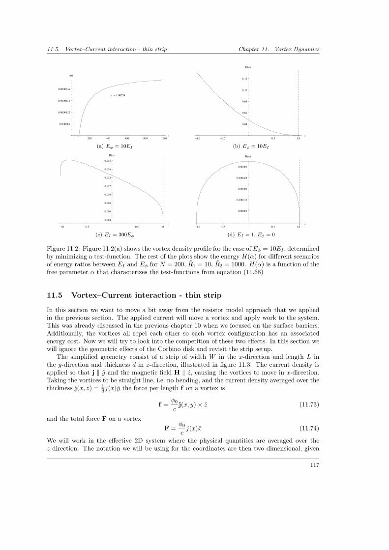
11.5. Vortex–Current interaction - thin strip Chapter 11. Vortex Dynamics

200 400 600 800 1000r

0.000063

0.0000632

0.0000634

0.0000636

nHrL

Α ® 1.00274

(a) Eφ = 10EI

-1.0 -0.5 0.5 1.0Α

0.04

0.06

0.08

0.10

0.12

HHΑL

(b) Eφ = 10EI

-1.0 -0.5 0.5 1.0Α

0.004

0.006

0.008

0.010

0.012

0.014

0.016

0.018

HHΑL

(c) EI = 300Eφ

-1.0 -0.5 0.5 1.0Α

0.00001

0.000015

0.00002

0.000025

0.00003

HHΑL

(d) EI = 1, Eφ = 0

Figure 11.2: Figure 11.2(a) shows the vortex density profile for the case of Eφ = 10EI , determinedby minimizing a test-function. The rest of the plots show the energy H(α) for different scenariosof energy ratios between EI and Eφ for N = 200, R1 = 10, R2 = 1000. H(α) is a function of thefree parameter α that characterizes the test-functions from equation (11.68)

11.5 Vortex–Current interaction - thin strip

In this section we want to move a bit away from the resistor model approach that we appliedin the previous section. The applied current will move a vortex and apply work to the system.This was already discussed in the previous chapter 10 when we focused on the surface barriers.Additionally, the vortices all repel each other so each vortex configuration has an associatedenergy cost. Now we will try to look into the competition of these two effects. In this section wewill ignore the geometric effects of the Corbino disk and revisit the strip setup.

The simplified geometry consist of a strip of width W in the x-direction and length L inthe y-direction and thickness d in z-direction, illustrated in figure 11.3. The current density isapplied so that j ‖ y and the magnetic field H ‖ z, causing the vortices to move in x-direction.Taking the vortices to be straight line, i.e. no bending, and the current density averaged over thethickness j(x, z) = 1

dj(x)y the force per length f on a vortex is

f =φ0

cj(x, y)× z (11.73)

and the total force F on a vortexF =

φ0

cj(x)x (11.74)

We will work in the effective 2D system where the physical quantities are averaged over thez-direction. The notation we will be using for the coordinates are then two dimensional, given

117

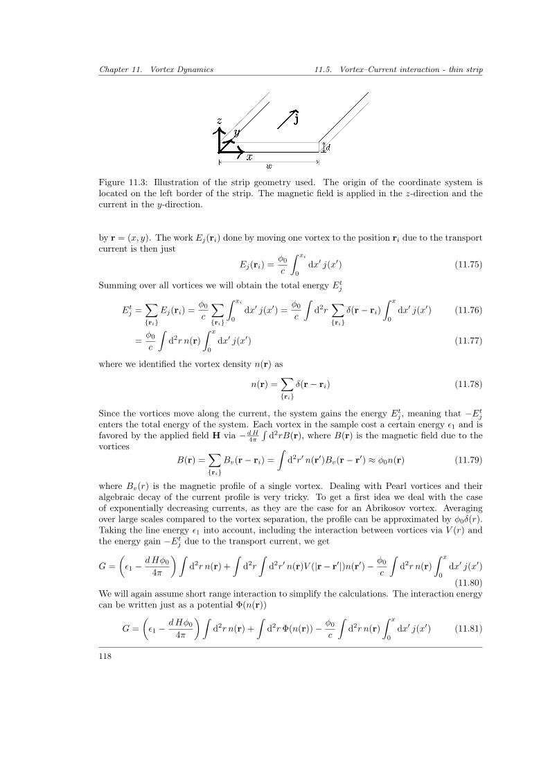
Chapter 11. Vortex Dynamics 11.5. Vortex–Current interaction - thin strip

Figure 11.3: Illustration of the strip geometry used. The origin of the coordinate system islocated on the left border of the strip. The magnetic field is applied in the z-direction and thecurrent in the y-direction.

by r = (x, y). The work Ej(ri) done by moving one vortex to the position ri due to the transportcurrent is then just

Ej(ri) =φ0

c

∫ xi

0

dx′ j(x′) (11.75)

Summing over all vortices we will obtain the total energy Etj

Etj =∑ri

Ej(ri) =φ0

c

∑ri

∫ xi

0

dx′ j(x′) =φ0

c

∫d2r

∑ri

δ(r− ri)

∫ x

0

dx′ j(x′) (11.76)

=φ0

c

∫d2r n(r)

∫ x

0

dx′ j(x′) (11.77)

where we identified the vortex density n(r) as

n(r) =∑ri

δ(r− ri) (11.78)

Since the vortices move along the current, the system gains the energy Etj , meaning that −Etjenters the total energy of the system. Each vortex in the sample cost a certain energy ε1 and isfavored by the applied field H via −dH4π

∫d2rB(r), where B(r) is the magnetic field due to the

vorticesB(r) =

∑ri

Bv(r− ri) =

∫d2r′ n(r′)Bv(r− r′) ≈ φ0n(r) (11.79)

where Bv(r) is the magnetic profile of a single vortex. Dealing with Pearl vortices and theiralgebraic decay of the current profile is very tricky. To get a first idea we deal with the caseof exponentially decreasing currents, as they are the case for an Abrikosov vortex. Averagingover large scales compared to the vortex separation, the profile can be approximated by φ0δ(r).Taking the line energy ε1 into account, including the interaction between vortices via V (r) andthe energy gain −Etj due to the transport current, we get

G =

(ε1 −

dHφ0

4π

)∫d2r n(r) +

∫d2r

∫d2r′ n(r)V (|r− r′|)n(r′)− φ0

c

∫d2r n(r)

∫ x

0

dx′ j(x′)

(11.80)We will again assume short range interaction to simplify the calculations. The interaction energycan be written just as a potential Φ(n(r))

G =

(ε1 −

dHφ0

4π

)∫d2r n(r) +

∫d2rΦ(n(r))− φ0

c

∫d2r n(r)

∫ x

0

dx′ j(x′) (11.81)

118

11.5. Vortex–Current interaction - thin strip Chapter 11. Vortex Dynamics

Variation leads to

δG

δn(r)=

(ε1 −

dHφ0

4π

)+ Φ′(n(r))− φ0

c

∫ x

0

dx′ j(x′)!= 0 (11.82)

The simplest form for the potential Φ(x) = c02 x

2 leads to

n(r) =1

c0

[(dHφ0

4π− ε1

)+φ0

c

∫ x

0

dx′ j(x′)

](11.83)

The density is constant in the absence of a current and increases for I > 0. The current densityof the system and the magnetic field due to the vortices are connected via Maxwell’s equation

∇×B =4π

cj(r) (11.84)

The current produced by an inhomogeneous vortex distribution can then be computes as

φ0∇× n(r)z = −φ0∂xn(r)y =4π

c djv(x)y (11.85)

where we assumed no line deformation of the vortices, i.e. no x-component of the magnetic field.In the static case the vortices do not move. This means the total current at the center of eachvortex, transport current j(x) and the current from vortices jv(x) satisfy

jv(x) + j(x) = 0 (11.86)

giving us the connection of n(x) and j(x) as

j(x) =φ0cd

4π∂xn(x) (11.87)

This simple connection leads to

φ0

c

∫ x

0

dx′ j(x′) =φ2

0d

4π(n(x)− n(0)) (11.88)

leading to a constant vortex density as the solution to equation (11.83). Even for an arbitrarylocal interaction Φ(n(r)) the equation (11.82) can be written as

Φ′(n(r))− φ20d

4πn(r) = F (n(r)) =

(dHφ0

4π− ε1

)− φ2

0d

4πn(0) (11.89)

where the right hand side is independent on the position, so the solution is just the constantprofile n(r) = n(0) with

F (n(0)) =

(dHφ0

4π− ε1

)− φ2

0d

4πn(0) (11.90)

So the vortex density does not seem to change due to a transport current. The constant densityalso means that there is no current jv = −∂xn(x) = 0 and in order for the configuration to bestatic this means that also j(x) = 0 being in conflict with

∫W0

dx j(x) = I > 0. The only placeleft for the current would be the outer borders of the sample. In this very simplified picturethe vortex lattice would stay constant for a non–vanishing current. The current itself wouldbe pushed to the borders of the sample. Obviously this picture needs to be modified once thecurrent densities at the boarders reaches the critical density. The model itself has not includedthe effect of vortices entering or leaving the sample explicitly.

119

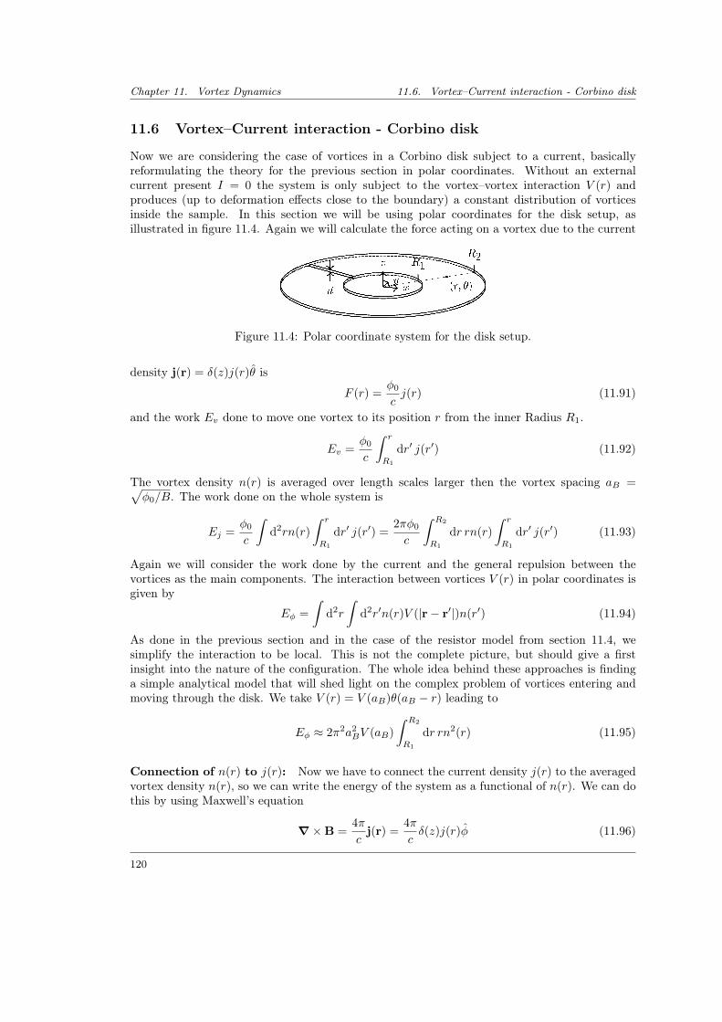
Chapter 11. Vortex Dynamics 11.6. Vortex–Current interaction - Corbino disk

11.6 Vortex–Current interaction - Corbino disk

Now we are considering the case of vortices in a Corbino disk subject to a current, basicallyreformulating the theory for the previous section in polar coordinates. Without an externalcurrent present I = 0 the system is only subject to the vortex–vortex interaction V (r) andproduces (up to deformation effects close to the boundary) a constant distribution of vorticesinside the sample. In this section we will be using polar coordinates for the disk setup, asillustrated in figure 11.4. Again we will calculate the force acting on a vortex due to the current

Figure 11.4: Polar coordinate system for the disk setup.

density j(r) = δ(z)j(r)θ is

F (r) =φ0

cj(r) (11.91)

and the work Ev done to move one vortex to its position r from the inner Radius R1.

Ev =φ0

c

∫ r

R1

dr′ j(r′) (11.92)

The vortex density n(r) is averaged over length scales larger then the vortex spacing aB =√φ0/B. The work done on the whole system is

Ej =φ0

c

∫d2rn(r)

∫ r

R1

dr′ j(r′) =2πφ0

c

∫ R2

R1

dr rn(r)

∫ r

R1

dr′ j(r′) (11.93)

Again we will consider the work done by the current and the general repulsion between thevortices as the main components. The interaction between vortices V (r) in polar coordinates isgiven by

Eφ =

∫d2r

∫d2r′n(r)V (|r− r′|)n(r′) (11.94)

As done in the previous section and in the case of the resistor model from section 11.4, wesimplify the interaction to be local. This is not the complete picture, but should give a firstinsight into the nature of the configuration. The whole idea behind these approaches is findinga simple analytical model that will shed light on the complex problem of vortices entering andmoving through the disk. We take V (r) = V (aB)θ(aB − r) leading to

Eφ ≈ 2π2a2BV (aB)

∫ R2

R1

dr rn2(r) (11.95)

Connection of n(r) to j(r): Now we have to connect the current density j(r) to the averagedvortex density n(r), so we can write the energy of the system as a functional of n(r). We can dothis by using Maxwell’s equation

∇×B =4π

cj(r) =

4π

cδ(z)j(r)φ (11.96)

120

11.6. Vortex–Current interaction - Corbino disk Chapter 11. Vortex Dynamics

and assuming that the magnetic field in the z direction inside the sample (z = 0) is only deter-mined by the vortex properties, meaning

Bz(z = 0) ≈ φ0n(r) (11.97)

Using the rotational symmetry, we can introduce the vector potential B = ∇ × A with A =f(r, z)θ. With the Coulomb gauge ∇A = 0 this results in the differential equation[

d2

dz2+

d

dr

1

r

d

drr

]f(r, z) = −4π

cδ(z)j(r) (11.98)

Following Pearl [125, 137], we can use the Hankel transform and introduce g(γ) via

f(r, z) =

∫ ∞0

dγ g(γ)J1(γr)e−γ|z| (11.99)

which solves the homogeneous part z > 0 and for z = 0 reduces to∫ ∞0

dγ γg(γ)J1(γr) =2π

cj(r) (11.100)

Using the inverse of the Hankel transform we can write the equation for g(γ) as

g(γ) =2π

c

∫ ∞0

dr rj(r)J1(γr) (11.101)

Computing the z-component of the magnetic field via

(∇×A)z =1

r

d

drrAφ ≈ φ0n(r) (11.102)

We can now use the fact that the Bessel-function J1(x) is the eigenfunction to the operator 1rddr r

with 1rddr rJ1(γr) = γJ0(γr) to get the relation

φ0n(r) ≈∫ ∞

0

dγ γg(γ)J0(γr) (11.103)

Again, using the properties of the Hankel transform of being its own inverse, we can now writeg(γ) dependent on n(r) via

g(γ) ≈ φ0

∫ ∞0

dr rn(r)J0(γr) (11.104)

Plugging this into the relation for the current density we get

j(r) ≈ c

2π

∫ ∞0

dγ γg(γ)J1(γr) =φ0c

2π

∫ ∞0

dγ γJ1(γr)

∫ ∞0

dr′ r′n(r′)J0(γr′) (11.105)

Using the identity∫ ∞0

dγ J0(γr′)γJ1(γr)e−γ|z| =k

8πr52 r′

32 (1− k2)

[k2(r2 − r′2 − z2)E(k) + 4rr′(1− k2)K(k)

](11.106)

≡ bz(r′, r, z) (11.107)

k =2√rr′√

z2 + (r + r′)2(11.108)

121

Chapter 11. Vortex Dynamics 11.6. Vortex–Current interaction - Corbino disk

(Prudnikov, Brychkov & Marichev Bd. II, p. 220, [160]), where the Elliptic integrals E(k) andK(k) are used in the Gradshteyn-Ryzhik definition, we can write

j(r) =φ0c

2π

∫ ∞0

dr′ r′n(r′)bz(r′, r, 0) (11.109)

Now that we have derived a relation between the current density j(r) and the vortex density n(r)we can now combine The energy functional for n(r) in the simplified form for the interactionthen reads

H[n(r)] = 2π2V (aB)

∫ R2

R1

dr rn2(r) + φ20

∫ R2

R1

dr rn(r)

∫ r

R1

dr′∫ R2

R1

dr′′ r′′n(r′′)bz(r′′, r′, 0)

(11.110)with the additional constrained that the number of vortices N in the sample stays fixed, meaning∫ R2

R1

dr rn(r) =N

2π

∫ R2

R1

dr j(r) = I (11.111)

Even after these simplifications the resulting energy functional in equation (11.110) is quitecomplicated due to the non–local nature of the current term. As we will see now, even a numericalapproach using a test function will not be feasible due to the divergent nature of the integralkernel bz(r, r′, z = 0) for r = r′.

Test functions: Using test functions that fulfill the constraints, we can try and get an idea ofthe shape of the vortex distribution. A simple distribution with only two parameters α and βcan be constructed as

nα,β(r) = (1− α− β)N

π(R22 −R2

1)+ α

N

2π(R2 −R1)

1

r+ β

3N

2π(R32 −R3

1)r (11.112)

consisting of a constant term, a 1/r decaying term and a linear increasing term. The expressionsatisfies the constrain

∫dr rn(r) = N/2π for all α and β. The second constrain∫ R2

R1

dr j(r) =φ0c

2π

∫ R2

R1

dr

∫ ∞0

dr′ r′n(r′)bz(r′, r, 0) = I (11.113)

leads to the algebraic equation for the coefficients α and β as

(1− α− β)c1 + αc2 + βc3 = I (11.114)

Here the numerical constants ci are given as

c1 =Nφ0c

2π2(R22 −R2

1)

∫ R2

R1

dr

∫ R2

R1

dr′ r′bz(r′, r, 0) (11.115)

c2 =Nφ0c

4π2(R2 −R1)

∫ R2

R1

dr

∫ R2

R1

dr′ bz(r′, r, 0) (11.116)

c3 =3Nφ0c

4π2(R32 −R3

1)

∫ R2

R1

dr

∫ R2

R1

dr′ r′2bz(r′, r, 0) (11.117)

The equation (11.114) can now be solved for β with

β =(1− α)c1 + αc2 − I

c1 − c3(11.118)

122

11.7. Discussion Chapter 11. Vortex Dynamics

The test profile is now only dependent on the parameter α. In order to guarantee that nα(r) ≥ 0for all R1 ≤ r ≤ R2 we can calculate the critical values αc1 and αc2 where the vortex densityactually vanishes

nαc1 (R1) = 0 nαc2 (R2) = 0 (11.119)

resulting in

αc1 =R1

(3c1R1(R1 +R2)− 2c3

(R2

1 +R1R2 +R22

)− I(R1 −R2)(R1 + 2R2)

)c1(R1 −R2)(R1 +R2)(2R1 +R2)− c2R1(R1 −R2)(R1 + 2R2) + c3 (R3

2 −R31)

(11.120)

αc2 =R2

(−3c1R2(R1 +R2) + 2c3

(R2

1 +R1R2 +R22

)+ I

(−2R2

1 +R1R2 +R22

))c1(R1 −R2)(R1 +R2)(R1 + 2R2) + c2R2 (−2R2

1 +R1R2 +R22) + c3 (R3

2 −R31)

(11.121)

Now plugging the test profile back into the energy functional, we will obtain the energy H(α)just as a function of the free parameter α. The first integral

∫dr′r′n2(r′) can be performed

analytically for the test-profile. The current interaction part however has no known analyticform. The minimization has to be performed numerically. As already hinted at above, thefunction bz(r, r′, z) is numerically not easy to tackle. The divergence in the integral kernel needsto be taken into account. Simple integration routines are not able to handle singularities in theintegrand. Usually, the function gets divided into intervals which become increasingly finer. Thesample points will get closer and closer to the singularity and will dominate the integral. Onealgorithm that can handle singularities is Monte–Carlo integration. Here the sample points arerandomly chosen from the integration domain as apposed to being on a fixed or adapted grid.The main disadvantage is the high run time compared to the low accuracy of the routine. Therun time for computing the energy for one fixed value α lies in the order of several hours. Severalparameters have to be examined, like the interaction energy versus the current strength, withoutprior knowledge where interesting effects may lie. The high run time makes an exploratoryapproach unfeasible.

11.7 Discussion

In this chapter the focus was on the dynamics of superconducting vortices in thin films. Mainlythe formation of flow lines and their bifurcation were of interest. In this chapter we exam-ined a collection of attempts at a simple analytical picture for the problem, made during thecollaboration via the German Israeli Foundation (GIF).

The problem itself is very complex. To simplify the geometry we have worked on either asimple strip configuration or with the Corbino disk setup. In the Meissner phase, i.e. in theabsence of vortices, we could calculate a very good approximation to the current distributionin the disk. Both the contribution due to the Meissner effect and due to an external appliedcurrent. Once one tries to include vortices in trying to construct a simple picture of the system,things become complicated quick. We saw that integrating out the free magnetic fields outsidethe disk, lead to a non–local interaction of the currents. Different parts of the disk, e.g. vorticesor more generally the current density, interact with each other via their generated and unshieldedmagnetic fields in the vacuum. Just analyzing the effect on the vortex density distribution due tothe current in the disk turns out to be difficult in itself. Additionally one would have to accountfor the exit and entry of vortices into the system, much like the surface barriers discussed in theprevious chapter 10.

Clean system In the clean system, i.e. ignoring disorder effects due to impurities in the system,our starting point was the construction of a simple picture for the vortex density distribution

123

Chapter 11. Vortex Dynamics 11.7. Discussion

and its interaction with the applied current density. In the Corbino disk setup the general flow ofthe vortices is radially outwards. The current is located at the borders of the disk and decreasestowards the middle and with it the force acting on a vortex, as we calculated and illustrated inequation (11.13) and (11.16). The vortices close to the border will move faster than the vorticescloser to the middle, effectively pushing them closer together in the r-direction. Starting witha dominant driving force, the vortices will move closer to each other until the force pushingthem together is of the order of their respective repulsion. Now the system wants to maximizethe distance between the vortices. Combined with the fact that the radial force in r-directionproduces an increasing gap between vortices in the tangential direction θ between different lines.This was the general narrative we tried to explore analytically. It is plausible to expect a pointwhere the creation of another flow line for the vortices will be favorable, being essentially abifurcation point. For the strip geometry and small currents we saw that the vortex lattice isstable and the currents are pushed towards the boundary. Generally in order to minimize energyloss due to vortex movement, the system will try to separate vortex and current density. Inthe Corbino disk setup that means that the majority of the current is located towards the innerring, while the majority of the vortices is located towards the outer ring. This radial change invortex density, illustrated in figure 11.2(a), will lead to a reorganization of the lattice structure.A rearranging in a dynamical picture can be the basis for bifurcation points. Approaching thismodel analytically has proven to be very difficult. Even in a very simplified version, the resultingfunctional turned out to neither be analytically nor numerically accessible, as we saw in section11.6

Disorder Additionally to the force of the current density and the interaction with the othervortices, a single vortex will also interact with a disorder background potential, e.g. due toimpurities. The clean system alone turned out to be not accessible, so disorder has been ignored.The reason it is mentioned here is because it was one idea to explain the flow line formation ofthe moving vortices. Much like a drop of water going down a rough tilted surface, as discussedby Narayan and Fisher, [161], the vortex will see a disorder energy landscape. When movingthrough the landscape the vortex will choose the path of least resistance. The flow line willroughen. In the absence of interaction, a second vortex starting in the vicinity of the first willfind the same path of low resistance following the first vortex. In case the driving force is muchstronger than the repulsion from the nearest vortex, the vortices should start following the valleysof the disordered landscape.

Time dependent Ginzburg–Landau theory Some numerical work has been done by Braunet al., [162], solving the time dependent Ginzburg–Landau equations for small strips with anapplied current. They see a change in the lattice density due to the current and the emergence ofdislocations, predicting instabilities and “fault lines”. Abandoning the idea of a simple analyticmodel, the direct simulation of the constriction using the time dependent GL theory seems tobe the most fruitful approach. However a simulation like this eludes the understanding of themechanisms leading to the bifurcations.

124

Part III

Appendix

A. Appendix: Model

A.1 XY quantum chain

In the case of quantum XY spins without the z-component, the FM and AFM case can bemapped onto each other and are therefore identical, [42]. The model of quantum XY spins ona one–dimensional chain with nearest–neighbor interaction is often referred to as the XX chaingiven as

HXX = −J2

∑i

(S+i S−i+1 + S−i S

+i+1

)(A.1)

and has been solved analytically for S = 1/2 in 1961 by Lieb et al. [163]. Looking at thecommutator relations for S±i

[Szi , S±j ] = ±δijS± [S+

i , S−i ] = 2δijS

zi (A.2)

we see that they have the meaning of raising S+i and lowering operators S−i . In the case of

S = 1/2 where the spin matrices are given by the Pauli matrices

σx =

(0 1

1 0

)σx =

(0 −ıı 0

)σz =

(1 0

0 −1

)(A.3)

Sαi = 12 σ

αi (setting ~ = 1 for convenience), we see that S±i behave both fermionic (on site)

S−i , S+i = 1

(S±i

)2

= 0 (A.4)

and bosonic (different sites)

[S+i , S

−j ] = [S+

i , S+j ] = [S−i , S

−j ] = 0 i 6= j (A.5)

as pointed out in [163]. Using the Jordan-Wigner transformation, which introduces the operators

c+i = S+i exp

−ıπ i−1∑j=1

S+j S−j

c−i = exp

ıπ i−1∑j=1

S+j S−j

S−i (A.6)

that behave fermionic on all sites, obeying the anti-commutator relations

c−i , c+j = δij c±i , c±j = 0 (A.7)

The Hamiltonian for the XX chain in these new fermionic operators

HXX = −J2

∑i

(c+i c−i+1 + c−i c

+i+1

)(A.8)

as shown in [163]. The Hamiltonian is now quadratic in completely fermionic operators anddescribes the spectrum of spinless free fermions, [42, 163]. The model can be diagonalized by asimple Fourier transform

c−k =1√N

∑i

c−i e−ıkri (A.9)

127

Appendix A. Appendix: Model A.1. XY quantum chain

leading toHXX =

∑k

ε(k)c+k c−k (A.10)

with ε(k) = −J cos(ka) and the lattice constant a, [42]. Inside the first Brillouin zone π/a ≤k ≤ π/a the highest and lowest energies are ±J with the Fermi energy EF laying in betweenat EF = 0 at the Fermi vector kF = ± π

2a . In the absence of a chemical potential (µ = 0) thesystem is half filled and the fermions at the Fermi energy, determine the relevant dynamics ofthe system at the momentum k = kF + q. The moving fermions have therefor a linear dispersionrelation with

ε(k) = ε(kF + q) = −J cos(±π2

+ qa) ≈ ±Jqa (A.11)

Another way of approaching the system of spinless free fermions was done by Haldane, [164],by looking at the continuous version of the free fermions and mapping it to a Luttinger–Liquid.This results in a linear dispersion relation as well.

The Jordan–Wigner transformation does not work for S 6= 1/2. For large spin S the XX chainmodel has been studied, e.g. in [165], using the Holstein–Primakoff transformation, [10, 166–168].Here the spin operators Sαi are represented via bosonic creation and annihilation operators a†and a measuring the deviation from the groundstate. Introducing a small magnetic field h in thex-direction to break the continuous symmetry, the groundstate lies in the x-direction. For spinS the deviation from the groudstate is measured by

Sxi = S − a†i ai (A.12)

−Szi + Syi = (2S − a†i ai)1/2ai (A.13)

−Szi − Syi = a†i (2S − a†i ai)1/2 (A.14)

[165], which can be expanded in terms of 1/S for large spins resulting in the approximate ex-pression for Syi as

Syi '√

2S

2ı

(ai − a†i

)(A.15)

The XX chain Hamiltonian for large spin is then of the simple form

HXX = −J∑i

(Sxi S

xi+1 + Syi S

yi+1

)(A.16)

' −JS2N + JS∑i

(2a†i ai +

1

2

(aiai+1 + a†i a

†i+1 − a†i ai+1 − aia†i+1

))+O(S0) (A.17)

Resulting in a Hamiltonian that is quadratic in the bosonic operators a, a† and can be diagonal-ized via Fourier and Bogoliubov transformations leading to the new bosonic operators bk and b†kwith

H =∑k

ε(k)b†k bk (A.18)

where the new dispersion relation is

ε(k) = 2JS√

1− cos(ka) ≈√

2JS|ka| (A.19)

[165], again leading to a linear dispersion relation for the excitations.

128

A.2. Kolezhuk mapping Appendix A. Appendix: Model

A.2 Kolezhuk mapping

In the case of the frustrated XY chain for large spin, Kolezhuk [43] was able to map the systemto a classical helimagnet with the action

A[ϕ] =1

2Teff

∫dx

∫dy

[1

4((∂xϕ)2 − θ2)2 + (∂yϕ)2 +

1

4(∂2xϕ)2

](A.20)

where effective temperature Teff is related to the spin S via Teff =√

32

1S , relating to the value

K0 used in our definition as

K0 =

√2

3S (A.21)

Even though we will be dealing with a purely classical system, this relation can be used toconnect it to the large spin case of frustrated one–dimensional quantum chains, [43].

Here we will reproduce the mapping procedure done by Kolezhuk in [43], with only slightdeviations. In his case, the quantum chain has antiferromagnetic interaction for both nearestneighbors and next–nearest neighbors.

H =∑n

(SnSn+1) + j(SnSn+2) (A.22)

with the parameter spin operators Sn = (Sxn, Syn,√

∆Szn). In the case of XY spins (∆ = 0),one can easily map the system to its ferromagnetic NN counterpart, by flipping every secondspin along the x-axis. The expansion around θ ≈ 0 and θ ≈ π show therefor the same criticalbehavior. We discussed this already in detail in chapter 2. Kolezhuk did the derivation for afinite ∆, we will here just focus on the ∆ = 0 case as it is the important one for this work.

Nonlinear sigma model

The first step is moving to coherent states, as described e.g. in [169, 170]. The Berry phase Φifor a single spin is written in terms of the vector ni parametrizing the coherent state at the sitei

Φi = S

∫dt∂tni(ni × ei)

1 + niei(A.23)

Here e describes an arbitrary unit vector, [43]. Choosing e1 = −n2 and e2 = −n1, the sum ofthe Berry phases of two neighboring spins works out to be

Φ12 = S

∫dt

n1 × n2

1− n1 · n2∂t(n2 − n1) (A.24)

Additionally Kolezhuk split the vector ni in a uniform magnetization mi and a staggered one livia

ni = mi + (−1)ili (A.25)

Both mi and li vary slowly close to the Lifshitz point j = 14 , making a continuum approximation

possible. Resulting in the action A as presented in [43].

A = 2πSQ+ S

∫dx

∫dt (l× ∂tl)− S2

∫dx

∫dt

3

4l2z + 2fαm

2α − 2εhα(∂xlα)2 +

1

8(∂2xxlα)2

129

Appendix A. Appendix: Model A.2. Kolezhuk mapping

with the topological charge Q = 14π

∫dt∫

dx l(∂xl× ∂tl). The notation used by Kolezhuk is

ε = j − 1

4fx,y = hx,y = 1 fz = 1 hz = 0 (A.26)

In the chiral regime with j > 1 and ε > 0 the pre-factor of (∂xlα)2 is negative. When doing anexpansion in the fields we then have to go up to at least the 4th order in the derivative in l,[43]. The m part can be integrated out and the imaginary time τ = 2ıSt can be introduced toproduce the Euclidean action

AE =1

2g0

∫dx

∫dτ

1

fα(l× ∂τ l)2

α − 4εhα(∂xlα)2 +1

4hα(∂2

xxlα)2 +3

2l2z

+ ı2πSQ (A.27)

as shown in [43], with the coupling constant g0 = 2/S.

Helimagnet

Equation (A.27) will now be mapped to a helimagnet following [43, 171]. Kolezhuk switches toangular variables lx + ıly = sin θeıϕ and lz = cos(θ). The field θ is massive and with θ = π

2 + ϑwe can expand the action in ϑ, [43].

AE = A[ϑ] +1

2g0

∫dx

∫dτ

1

fz(∂τϕ)2[1 + (fz − 2)ϑ2]

+ (1− ϑ2)

[−4ε(∂xϕ)2 +

1

4(∂xϕ)4 +

1

4(∂2xxϕ)2

]+ ı2πSQ (A.28)

A[ϑ] =1

2g0

∫dx

∫dτ

(∂τϑ)2 − 3

2ϑ2

(A.29)

Dealing with the special case ∆ = 0 simplifies equation (A.29) compared to the ∆ 6= 0 case in[43]. Here it is easy to see that ϑ is a massive field that will rescale the coupling parameters.Kolezhuk applied Polyakov-type RG to the ∆ 6= 0 model resulting to the planar helimagnet,dependent only on the in-plane angle ϕ, [43]. Setting ∆ = 0 afterward results in

A[ϕ] =1

2Teff

∫dx

∫dy

(∂yϕ)2 + V [ϕ]

(A.30)

V [ϕ] =1

4

[(∂xϕ)2 − 8ε

]2 (A.31)

with the effective temperature Teff =√

3/2 1S and the “spatial” dimension y =

√3/2τ . The

topological charge Q is dropped when moving to the planar model.

130

B. Appendix: Renormalization Group

B.1 Vortex core energy integral

Here the analytic results for the core energy integrals are listed. The vortex profile ansatz

φv(x, y) = arcsin(ζ)θ(x) + [π − arcsin(ζ)]θ(−x) (B.1)

where ζ = λy/√x4 + λ2y2 is used to approximate the core energy

Ecore(λ) =K0

2

∫x

[φ2y +

1

4(φ2xx + φ4

x)

](B.2)

The diverge for small distances, so the small scale cutoff a = 1 is used, via∫x7→ 4

∫∞1

d2x Theenergy can be split into three different integrals as

Ecore = 4K0

2

[∫ ∞1

d2x (∂yφv)2︸ ︷︷ ︸

=Eφ2y

+1

4

∫ ∞1

d2x (∂2xφv)

2︸ ︷︷ ︸Eφ2

xx

+1

4

∫ ∞1

d2x (∂xφv)4︸ ︷︷ ︸

Eφ4x

](B.3)

The integrals can be solved analytically. The results are given in the equations (B.4), (B.5) and(B.6). They were obtained using Mathematica and checked by comparing the analytic expressionswith their numeric counterparts.

Eφ2y

=

∫ ∞1

d2x (∂yφv)2

=λ

4(π − 2 arctan(λ))

+

√λ

4√

2

[arctan

(1−

√2

λ

)− arctan

(√2

λ+ 1

)− arccoth

(λ+ 1√

2λ

)+ π

](B.4)

Eφ2xx

=

∫ ∞1

d2x (∂2xφv)

2

=5π

2√

2λ3/2+

5

4√

2λ3/2ln

(λ−√

2λ+ 1

λ+√

2λ+ 1

)+

5

2√

2λ3/2arctan

(1−

√2

λ

)

− 5

2√

2λ3/2arctan

(1 +

√2

λ

)− 4λ2

3 (λ2 + 1)2 +

1

3 (λ2 + 1)+π

λ− 2

λarctan(λ) (B.5)

131

Appendix B. Appendix: Renormalization Group B.2. Fourier transform in x-direction

Eφ4x

=

∫ ∞1

d2x (∂xφv)4

=3λ2

4 (λ2 + 1)2 +

π√

2λ

(λ2 + 1)2 +

5

12 (λ2 + 1)2 +

√λ

4√

2 (λ2 + 1)2 arctan

(1−√

2λ)

−√λ

4√

2 (λ2 + 1)2 arctan

(1 +√

2λ)

+2λ

(λ2 + 1)2 arccot(λ) +

1

λ (λ2 + 1)2 arccot(λ)

+2(−1)3/4

√λ

(λ2 + 1)2 arctanh

(4√−1√λ

)+

2 4√−1√λ

(λ2 + 1)2 arctanh

((−1)3/4

√λ

)+

√λ

4√

2 (λ2 + 1)2 arccoth

(λ+ 1√

2λ

)+

πλ5/2

√2 (λ2 + 1)

2 +π√

2λ3/2 (λ2 + 1)2

+λ5/2

8√

2 (λ2 + 1)2 arctan

(1−√

2λ)− λ5/2

8√

2 (λ2 + 1)2 arctan

(1 +√

2λ)

+1

8√

2λ3/2 (λ2 + 1)2 arctan

(1−√

2λ)− 1

8√

2λ3/2 (λ2 + 1)2 arctan

(1 +√

2λ)

+(−1)3/4λ5/2

(λ2 + 1)2 arctanh

(4√−1√λ

)+

4√−1λ5/2

(λ2 + 1)2 arctanh

((−1)3/4

√λ

)+

(−1)3/4

λ3/2 (λ2 + 1)2 arctanh

(4√−1√λ

)+

4√−1

λ3/2 (λ2 + 1)2 arctanh

((−1)3/4

√λ

)+

λ5/2

8√

2 (λ2 + 1)2 arccoth

(λ+ 1√

2λ

)+

1

8√

2λ3/2 (λ2 + 1)2 arccoth

(λ+ 1√

2λ

)+

λ3

(1 + λ2)2 arccot(λ) (B.6)

Here the convention introduced in the Software Mathematica is used, where

4√−1 ≡ 1√

2+

ı√2

(−1)3/4 ≡ − 1√2

+ı√2. (B.7)

This notation was adopted to shorten the already very lengthy expression.The minimum of the function Ecore(λ) in respect to λ can then be determined numerically

resulting in

Ecore = 2.38K0 λ = 2.38 (B.8)

The nicer notation of κ = 1/λ has been used in the main text and the publication [40].

B.2 Fourier transform in x-direction

Here the details concering the computation of the correlator

G(x,y) =

∫dkx2π

d3/2k⊥(2π)3/2

k2x

k2⊥ + 1

4k4x

eıkxxeık⊥y =1

yf

(x2

y

)(B.9)

are presented.We can perform the Fourier transform in the x-direction given by

M(k⊥, x) =

∫dkx2π

k2x

k2⊥ + 1

4k4x

eıkxx →√

8

∫dk′x2π

k′x2

k2⊥ + k′x

4 eık′xx

′(B.10)

132

B.3. Calculating the constant pre-factor f(0) Appendix B. Appendix: Renormalization Group

where we used the scaling k′x = kx/√

2 and x′ =√

2x to remove the pre-factor of 1/4 in front ofthe k4

x part.

M(k⊥, x) =

∫dkx2π

k2x

k2⊥ + k4

x

eıkxx =

∫dkx2π

k2x∏

i(kx − ki)eıkxx =

∮kx2π

k2x∏

i(kx − ki)eıkxx

where after identifying the roots ki = ±eıπ/4√k⊥,±eı3π/4

√k⊥ we switch to a contour integral

for x > 0 by adding a circle path in the upper complex plane. The two roots in the upper planeare k1 = eıπ/4

√k⊥ = 1/

√2(1 + ı)

√k⊥ and k2 = eı3π/4

√k⊥ = 1/

√2(−1 + ı)

√k⊥. Applying

Cauchy’s residual theorem, we can perform the contour integral

M(k⊥, x) = ı

[k2

1∏i 6=1(k1 − ki)

eık1x +k2

2∏i 6=2(k2 − ki)

eık2x

]

=1

4

√2

k⊥e−√k⊥2 x

[(1

2+ ı

1

2)eı√k⊥2 x − (−1

2+ ı

1

2)e−ı

√k⊥2 x

]=

1

4

√2

k⊥e−√k⊥2 x

[cos(

√k⊥2x)− sin(

√k⊥2x)

]

After scaling the variables back to their original, by multiplying with√

8 and scaling x →√

2xwe arrive at the Fourier transform

M(k⊥, x) =1√k⊥

e−√k⊥x

[cos(

√k⊥x)− sin(

√k⊥x)

](B.11)

B.3 Calculating the constant pre-factor f(0)

By looking at the scaling relations of the integral in equation (B.9), we can write our problem as∫dkx2π

d3/2k⊥(2π)3/2

k2x

k2⊥ + 1

4k4x

eıkxxeık⊥y =

∫d3/2k⊥(2π)3/2

M(k⊥, x)eık⊥y =1

yf(x2

y) (B.12)

So with M(k⊥, 0) = 1/√k⊥ one can calculate the value for f(0) = A = const with

f(0)

y=

∫d3/2k⊥(2π)3/2

1√k⊥

eık⊥y (B.13)

looking at the 3D and 4D polar coordinates for the integration we can generalize a relation ford-dimensions which can then be used for our fractional d = 3/2. We use the general pre-factorKd = 2πd/2/Γ(d/2)

3D :

∫d3xeıkx =

∫ ∞0

dr

∫ π

0

dφ1

∫ 2π

0

dφ2r2 sin(φ1)eıkx cos(φ1) = K2

∫ ∞0

dr

∫ π

0

dφ1r2 sin(φ1)eıkx cos(φ1)

4D :

∫d4xeıkx = K3

∫ ∞0

dr

∫ π

0

dφ1r3 sin2(φ1)eıkx cos(φ1)

d :

∫ddxeıkx = Kd−1

∫ ∞0

dr

∫ π

0

φ1rd−1 sind−2(φ1)eıkx cos(φ1)

133

Appendix B. Appendix: Renormalization Group B.3. Calculating the constant pre-factor f(0)

We can even perform the integration over the angular part (in general d > 1), where we willswitch to z = cos(φ) using sin(arccos(z)) =

√1− z2

∫ π

0

dφ sind−2(φ)eık⊥ cos(φ) =

∫ 1

−1

dz(1− z2)d−3

2 eık⊥z =

∞∑n=0

(−1)nk2n⊥

(2n)!

∫ 1

−1

dz z2n(1− z2)d−3

2

=

∞∑n=0

(−1)nk2n⊥

(2n)!

∫ 1

0

dxx(n+ 12 )−1(1− x)

d−12 −1 =

∞∑n=0

(−1)nk2n⊥

(2n)!B(n+

1

2,d− 1

2)

where, after switching to x = z2, we identified the Beta function B(x, y) with

B(x, y) =

∫ 1

0

dz zx−1(1− z)y−1 =Γ(x)Γ(y)

Γ(x+ y)

Using the doubling Formula for the Gamma function

Γ(2n+ 1) =1√2π

22n+ 12 Γ(n+

1

2)Γ(n+ 1) =

22n

√π

Γ(n+1

2)n!

we can rewrite the sum

∞∑n=0

(−1)nk2n⊥

(2n)!B(n+

1

2,d− 1

2) =

∞∑n=0

(−1)nk2n⊥

Γ(n+ 12 )Γ(d−1

2 )

Γ(2n+ 1)Γ(n+ d2 )

=√πΓ(

d− 1

2)∑n

(−k

2⊥4

)n1

n!

1

Γ(n+ d2 )

=√π

Γ(d−1

2

)Γ(d2

) 0F1(d

2,−k

2⊥4

)

Where we could identify the series representation of the confluent hypergeometric function0F1(α;x)

0F1(a;x) =

∞∑n=0

xn

n!

Γ(a)

Γ(a+ n)(B.14)

giving us the general result∫ π

0

dφ sind−2(φ)eık⊥ cos(φ) =√π

Γ(d−1

2

)Γ(d2

) 0F1(d

2,−k

2⊥4

) (B.15)

So in our case we get

f(0)

y=

K1/2

(2π)3/2

∫ ∞0

dk⊥

∫ π

0

dφ1√

sin(φ)eık⊥y cos(φ) =

1

y

K1/2

(2π)3/2

∫ ∞0

dk⊥

∫ π

0

dφ1√

sin(φ)eık⊥ cos(φ)

=1

y

K1/2

(2π)3/2

∫ ∞0

dk⊥

√π

Γ( 14 )

Γ( 34 )

0F1(3

4,−k

2⊥4

)

︸ ︷︷ ︸

=π

=1

y

K1/2π

(2π)3/2=

1

y

2π5/4

(2π)3/2Γ(

14

) =1

y

1√2π1/4Γ

(14

)Giving us the result f(0)−1 =

√2π

14 Γ(

14

)f(0) =

1√2π

14 Γ(

14

) (B.16)

134

B.4. Calculating the f(z → ∞) limit Appendix B. Appendix: Renormalization Group

B.4 Calculating the f(z →∞) limit

One can even perform the y → 0 limit of the function leading to the integral

I = limy→0

f(x2

y )

y=

∫dkx2π

d3/2k⊥(2π)3/2

k2x

k2⊥ + 1

4k4x

eıkxx =K3/2

(2π)3/2

∫ ∞0

dk⊥√k⊥M(k⊥, x) (B.17)

Using the Fourier transformation in x-directionM(k⊥, x) = 1√k⊥e−√k⊥x

[cos(√k⊥x)− sin(

√k⊥x)

]from equation (B.11) the integral becomes

I =K3/2

(2π)3/2

∫ ∞0

dk⊥e−√k⊥x

[cos(

√k⊥x)− sin(

√k⊥x)

]=

1

x2

K3/2

(2π)3/2

∫ ∞0

dk⊥e−√k⊥[cos(

√k⊥)− sin(

√k⊥)

]=

1

x2

K3/2

(2π)3/2

∫ ∞0

dz(2z)e−z [cos(z)− sin(z)] =1

x2

K3/2

(2π)3/2(−2∂a)

∫ ∞0

dz e−az [cos(z)− sin(z)]

∣∣∣∣∣a=1

=1

x2

K3/2

(2π)3/2(−2∂a)L[cos](a)− L[sin](a)

where we introduced the variable transform z =√k⊥. The Laplace transforms L[. . . ] are given

by

L[cos](a) =a

1 + a2∂aL[cos]

∣∣∣a=1

=

[1

1 + a2− 2a2

(1 + a2)2

]a=1

= 0

L[sin](a) =1

1 + a2∂aL[sin]

∣∣∣a=1

= − 2a

(1 + a2)2

∣∣∣a=1

= −1

2

leading to

limy→0

f(x2

y )

y= − 1

x2

K3/2

(2π)3/2f(z →∞) = −1

z

K3/2

(2π)3/2(B.18)

B.5 Solving the full Fourier transform

Using the results for the Fourier transform M(k⊥, x) in x-direction from equation (B.11) andthe general result for the angular integration of the k⊥ integral from equation (B.15) the full

135

Appendix B. Appendix: Renormalization Group B.6. Solving f(z) via ODE

problem can be rewritten as

f(z = x2

y )

y=

∫dkx2π

d3/2k⊥(2π)3/2

k2x

k2⊥ + 1

4k4x

eıkxxeık⊥y

=K1/2

(2π)3/2

√π

Γ( 14 )

Γ( 34 )

∫ ∞0

dk⊥√k⊥M(k⊥, x)0F1(

3

4,− (k⊥y)2

4)

=K1/2

(2π)3/2

√π

Γ( 14 )

Γ( 34 )

∫ ∞0

dk⊥e−√k⊥x(cos(

√k⊥x)− sin(

√k⊥x))0F1(

3

4,− (k⊥y)2

4)

=1

y

K1/2

(2π)3/2

√π

Γ( 14 )

Γ( 34 )

∫ ∞0

dk⊥e−√k⊥z(cos(

√k⊥z)− sin(

√k⊥z))0F1(

3

4,− (k⊥)2

4)

=1

y

K1/2

(2π)3/2

√π

Γ( 14 )

Γ( 34 )

∫ ∞0

dt (2t)e−t√z(cos(t

√z)− sin(t

√z))0F1(

3

4,− t

4

4)

=1

y

z3/4

4π14

(I− 3

4

(z2

)−LLL− 3

4

(z2

))with Iν(x) the modified Bessel function of the first kind and LLLν(x) the modified Struve function.

B.6 Solving f(z) via ODE

We can write down the differential equation for the correlator being the saddle point equationsof the form

(∂4x −∆⊥)G(x, y⊥) = 0 (B.19)

The field correlator G = 〈φφ〉 and the correlator of the derivatives G = 〈∂xφ∂xφ〉 are relatedvia the second derivative in x. Since ∂x commutes with ∆⊥, both functions are solutions tothe differential equation above. So we can start looking for a function of the form f(x2/y)/ysatisfying the above differential equation.

First we have to find a general form for the Laplace operator ∆⊥ which works in d = 3/2. Inorder to do so, we will look at the radial part of the Laplace operator in several known dimensionsand generalize it for d-dimensions

2D : ∆r =1

r∂r (r∂rf) 3D : ∆r =

1

r2∂r(r2∂rf

)4D : ∆r =

1

r3∂r(r3∂rf

)d : ∆r =

1

rd−1∂r(rd−1∂rf

)=

(d− 1

r∂r + ∂2

r

)f

With the ansatz G(x, r) = 1rf(x

2

r ) found by looking at the scaling relations in the integral fromof G, we can start to rewrite the differential equation

(1

4∂4x −

1

2r∂r − ∂2

r )1

rf(x2

r) = 0

using z = x2/r to compactify the notation, we can write the different parts of the partial

136

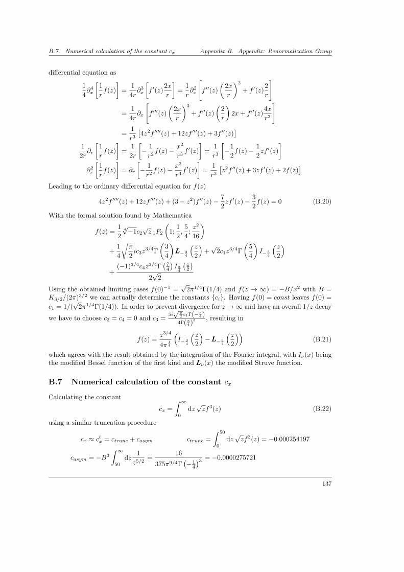
B.7. Numerical calculation of the constant cx Appendix B. Appendix: Renormalization Group

differential equation as

1

4∂4x

[1

rf(z)

]=

1

4r∂3x

[f ′(z)

2x

r

]=

1

r∂2x

[f ′′(z)

(2x

r

)2

+ f ′(z)2

r

]

=1

4r∂x

[f ′′′(z)

(2x

r

)3

+ f ′′(z)

(2

r

)2x+ f ′′(z)

4x

r2

]

=1

r3

[4z2f ′′′′(z) + 12zf ′′′(z) + 3f ′′(z)

]1

2r∂r

[1

rf(z)

]=

1

2r

[− 1

r2f(z)− x2

r3f ′(z)

]=

1

r3

[−1

2f(z)− 1

2zf ′(z)

]∂2r

[1

rf(z)

]= ∂r

[− 1

r2f(z)− x2

r3f ′(z)

]=

1

r3

[z2f ′′(z) + 3zf ′(z) + 2f(z)

]Leading to the ordinary differential equation for f(z)

4z2f ′′′′(z) + 12zf ′′′(z) + (3− z2)f ′′(z)− 7

2zf ′(z)− 3

2f(z) = 0 (B.20)

With the formal solution found by Mathematica

f(z) =1

24√−1c2

√z 1F2

(1;

1

2,

5

4;z2

16

)+

1

4

√π

2ic3z

3/4Γ

(3

4

)LLL− 3

4

(z2

)+√

2c1z3/4Γ

(5

4

)I− 3

4

(z2

)+

(−1)3/4c4z3/4Γ

(74

)I 3

4

(z2

)2√

2

Using the obtained limiting cases f(0)−1 =√

2π1/4Γ(1/4) and f(z → ∞) = −B/x2 with B =K3/2/(2π)3/2 we can actually determine the constants ci. Having f(0) = const leaves f(0) =

c1 = 1/(√

2π1/4Γ(1/4)). In order to prevent divergence for z →∞ and have an overall 1/z decay

we have to choose c2 = c4 = 0 and c3 =5i√

π2 c1Γ(− 5

4 )4Γ( 3

4 )3 , resulting in

f(z) =z3/4

4π14

(I− 3

4

(z2

)−LLL− 3

4

(z2

))(B.21)

which agrees with the result obtained by the integration of the Fourier integral, with Iν(x) beingthe modified Bessel function of the first kind and LLLν(x) the modified Struve function.

B.7 Numerical calculation of the constant cx

Calculating the constant

cx =

∫ ∞0

dz√zf3(z) (B.22)

using a similar truncation procedure

cx ≈ ctx = ctrunc + casym ctrunc =

∫ 50

0

dz√zf3(z) = −0.000254197

casym = −B3

∫ ∞50

dz1

z5/2=

16

375π9/4Γ(− 1

4

)3 = −0.0000275721

137

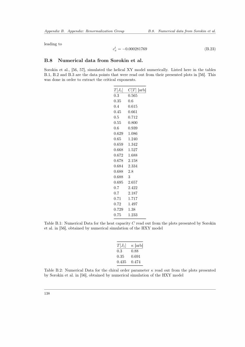
Appendix B. Appendix: Renormalization Group B.8. Numerical data from Sorokin et al.

leading toctx = −0.000281769 (B.23)

B.8 Numerical data from Sorokin et al.

Sorokin et al., [56, 57], simulated the helical XY model numerically. Listed here in the tablesB.1, B.2 and B.3 are the data points that were read out from their presented plots in [56]. Thiswas done in order to extract the critical exponents.

T [J1] C[T ] [arb]0.3 0.5650.35 0.60.4 0.6150.45 0.6610.5 0.7120.55 0.8000.6 0.9390.629 1.0860.65 1.2400.659 1.3420.668 1.5270.672 1.6880.678 2.1580.684 2.3340.688 2.80.688 30.695 2.6570.7 2.4220.7 2.1870.71 1.7170.72 1.4970.729 1.380.75 1.233

Table B.1: Numerical Data for the heat capacity C read out from the plots presented by Sorokinet al. in [56], obtained by numerical simulation of the HXY model

T [J1] κ [arb]0.3 0.880.35 0.6910.435 0.474

Table B.2: Numerical Data for the chiral order parameter κ read out from the plots presentedby Sorokin et al. in [56], obtained by numerical simulation of the HXY model

138

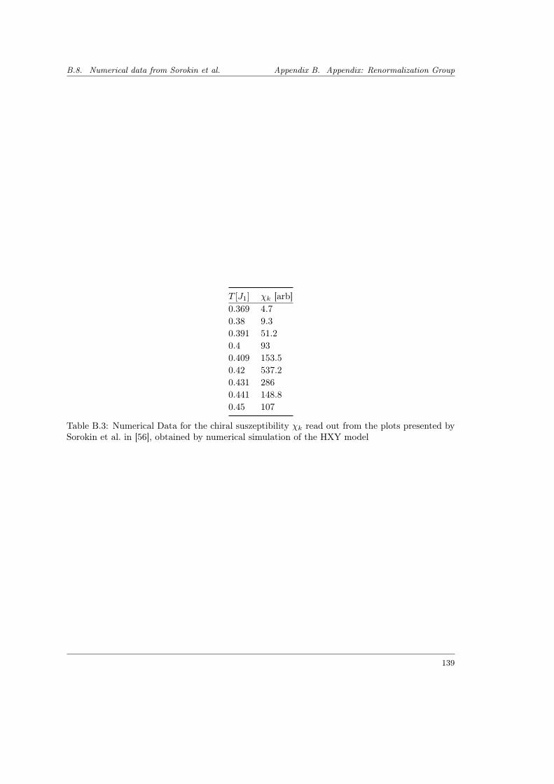
B.8. Numerical data from Sorokin et al. Appendix B. Appendix: Renormalization Group

T [J1] χk [arb]0.369 4.70.38 9.30.391 51.20.4 930.409 153.50.42 537.20.431 2860.441 148.80.45 107

Table B.3: Numerical Data for the chiral suszeptibility χk read out from the plots presented bySorokin et al. in [56], obtained by numerical simulation of the HXY model

139

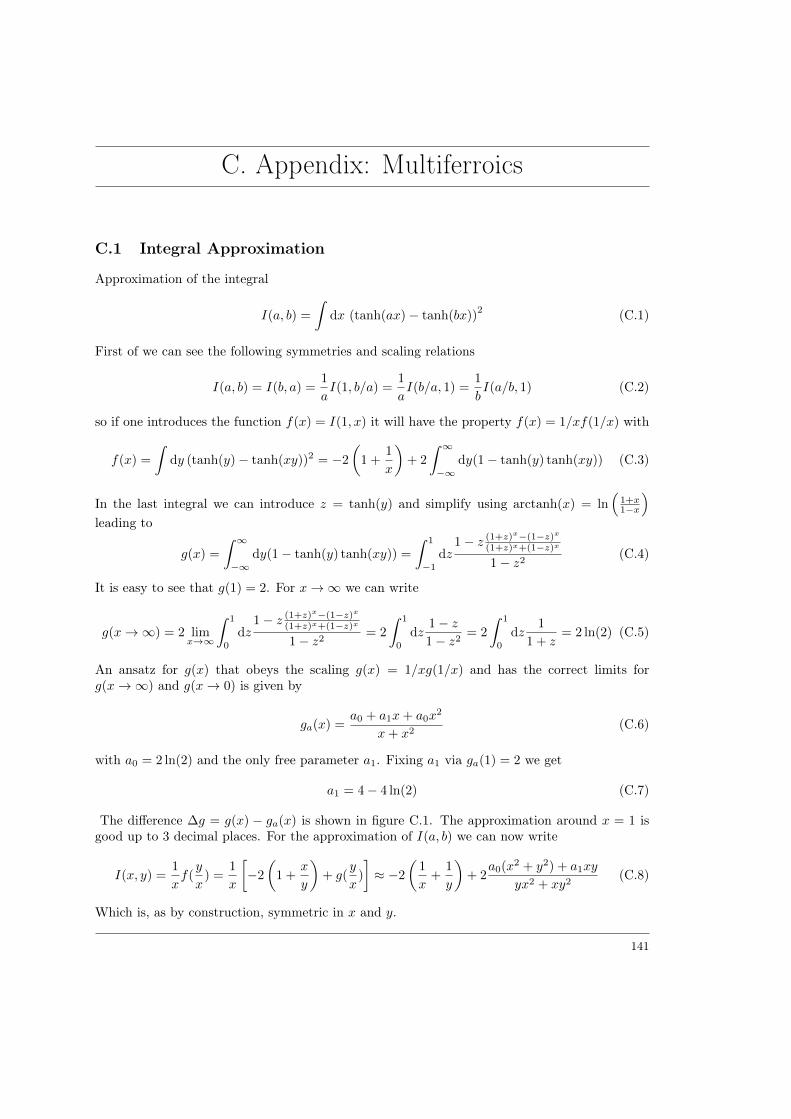
C. Appendix: Multiferroics

C.1 Integral Approximation

Approximation of the integral

I(a, b) =

∫dx (tanh(ax)− tanh(bx))

2 (C.1)

First of we can see the following symmetries and scaling relations

I(a, b) = I(b, a) =1

aI(1, b/a) =

1

aI(b/a, 1) =

1

bI(a/b, 1) (C.2)

so if one introduces the function f(x) = I(1, x) it will have the property f(x) = 1/xf(1/x) with

f(x) =

∫dy (tanh(y)− tanh(xy))2 = −2

(1 +

1

x

)+ 2

∫ ∞−∞

dy(1− tanh(y) tanh(xy)) (C.3)

In the last integral we can introduce z = tanh(y) and simplify using arctanh(x) = ln(

1+x1−x

)leading to

g(x) =

∫ ∞−∞

dy(1− tanh(y) tanh(xy)) =

∫ 1

−1

dz1− z (1+z)x−(1−z)x

(1+z)x+(1−z)x

1− z2(C.4)

It is easy to see that g(1) = 2. For x→∞ we can write

g(x→∞) = 2 limx→∞

∫ 1

0

dz1− z (1+z)x−(1−z)x

(1+z)x+(1−z)x

1− z2= 2

∫ 1

0

dz1− z1− z2

= 2

∫ 1

0

dz1

1 + z= 2 ln(2) (C.5)

An ansatz for g(x) that obeys the scaling g(x) = 1/xg(1/x) and has the correct limits forg(x→∞) and g(x→ 0) is given by

ga(x) =a0 + a1x+ a0x

2

x+ x2(C.6)

with a0 = 2 ln(2) and the only free parameter a1. Fixing a1 via ga(1) = 2 we get

a1 = 4− 4 ln(2) (C.7)

The difference ∆g = g(x) − ga(x) is shown in figure C.1. The approximation around x = 1 isgood up to 3 decimal places. For the approximation of I(a, b) we can now write

I(x, y) =1

xf(y

x) =

1

x

[−2

(1 +

x

y

)+ g(

y

x)

]≈ −2

(1

x+

1

y

)+ 2

a0(x2 + y2) + a1xy

yx2 + xy2(C.8)

Which is, as by construction, symmetric in x and y.

141

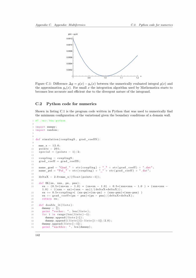
Appendix C. Appendix: Multiferroics C.2. Python code for numerics

0.9 1.0 1.1 1.2x

0.0002

0.0004

0.0006

0.0008

0.0010

0.0012

g(x) - ga(x)

Figure C.1: Difference ∆g = g(x) − ga(x) between the numerically evaluated integral g(x) andthe approximation ga(x). For small x the integration algorithm used by Mathematica starts tobecomes less accurate and efficient due to the divergent nature of the integrand.

C.2 Python code for numerics

Shown in listing C.1 is the program code written in Python that was used to numerically findthe minimum configuration of the variational given the boundary conditions of a domain wall.

1 #! / usr /bin /python2

3 import numpy ;4 import random ;5

6

7 de f s imu la t i on ( coupl ingS , grad_coef fS ) :8

9 max_x = 12 . 0 ;10 po in t s = 201 ;11 s p e c i a l = ( po in t s − 1) /2 ;12

13 coup l ing = coupl ingS ;14 grad_coef f = grad_coef fS ;15

16 name_grad = "Grad_" + s t r ( coup l ing ) + "_" + s t r ( grad_coef f ) + " . dat" ;17 name_pol = "Pol_" + s t r ( coup l ing ) + "_" + s t r ( grad_coef f ) + " . dat" ;18

19 deltaX = 2.0∗max_x/( f l o a t ( po ints −1) ) ;20

21 de f IK(xn , xnn , pn , pnn ) :22 en = (0 . 5∗ ( xn∗xn − 1 . 0 ) ∗ ( xn∗xn − 1 . 0 ) + 0 . 5∗ ( xnn∗xnn − 1 .0 ) ∗ ( xnn∗xnn −

1 . 0 ) + ( ( xnn − xn ) ∗( xnn − xn ) ) /( deltaX∗deltaX ) ) ;23 en += 0.5∗ coup l ing ∗( (xn−pn) ∗(xn−pn) + (xnn−pnn) ∗(xnn−pnn) )24 en += grad_coef f ∗(pn − pnn) ∗(pn − pnn) /( deltaX∗deltaX ) ;25 r e turn en ;26

27 de f double_it ( l i s t e ) :28 dummy = [ ] ;29 pr in t " vorher : " , l en ( l i s t e ) ;30 f o r i in range ( l en ( l i s t e )−1) :31 dummy. append ( l i s t e [ i ] ) ;32 dummy. append ( ( l i s t e [ i ]+ l i s t e [ i +1]) /2 . 0 ) ;33 dummy. append ( l i s t e [−1]) ;34 pr in t "nachher : " , l en (dummy) ;

142

C.2. Python code for numerics Appendix C. Appendix: Multiferroics

35 r e turn l i s t (dummy) ;36

37 grad i en t = [ ] ;38 po l a r i z a t i o n = [ ] ;39

40 de f save (name_g , name_p) :41 f g = open (name_g , "w" ) ;42 fp = open (name_p , "w" ) ;43 f o r i in range ( l en ( g rad i en t ) ) :44 f g . wr i t e ( s t r (−max_x + f l o a t ( i ) ∗deltaX ) + "\ t " + s t r ( g rad i en t [ i ] ) + "\n" ) ;45 fp . wr i t e ( s t r (−max_x + f l o a t ( i ) ∗deltaX ) + "\ t " + s t r ( p o l a r i z a t i o n [ i ] ) + "\n" )

;46 f g . c l o s e ( ) ;47 fp . c l o s e ( ) ;48

49 f o r i in range ( po in t s ) :50 i f ( i < s p e c i a l ) :51 grad i en t . append ( 1 . 0 ) ;# + random . uniform ( −0 .01 ,0 .01) ) ;52 po l a r i z a t i o n . append (−1.0) ;53 e l s e :54 grad i en t . append (−1.0) ;# + random . uniform ( −0 .01 ,0 .01) ) ;55 po l a r i z a t i o n . append ( 1 . 0 ) ;56

57 # Boundary cond i t i on s58 grad i en t [ s p e c i a l ] = 0 . 0 ;59 po l a r i z a t i o n [ s p e c i a l ] = 0 . 0 ;60

61

62 h = 0 . 2 ;63 changes = True ;64 dx_stop = 0 . 0001 ;65 HdDx_stop = 0 . 0001 ;66

67

68 whi le True :69 #break ;70 pr in t "DX: " , deltaX ;71 pr in t "h : " , h ;72 pr in t "h/DX: " , h/deltaX ;73 changes = True ;74 whi le changes :75 changes = False ;76 grad_neu = l i s t ( g rad i en t ) ;77 pol_neu = l i s t ( p o l a r i z a t i o n ) ;78

79 # s t a r t and end po int80 f 0 = IK( grad i en t [ 0 ] , g rad i en t [ 1 ] , p o l a r i z a t i o n [ 0 ] , p o l a r i z a t i o n [ 1 ] ) ;81 fp = IK( grad i en t [0 ]+h , g rad i en t [ 1 ] , p o l a r i z a t i o n [ 0 ] , p o l a r i z a t i o n [ 1 ] ) ;82 fn = IK( grad i en t [0]−h , g rad i en t [ 1 ] , p o l a r i z a t i o n [ 0 ] , p o l a r i z a t i o n [ 1 ] ) ;83 pp = IK( grad i en t [ 0 ] , g rad i en t [ 1 ] , p o l a r i z a t i o n [0 ]+h , p o l a r i z a t i o n [ 1 ] ) ;84 pn = IK( grad i en t [ 0 ] , g rad i en t [ 1 ] , p o l a r i z a t i o n [0]−h , p o l a r i z a t i o n [ 1 ] ) ;85

86 i f fp <= fn and fp < f0 and fp <= pp and fp <= pn and ( g rad i en t [ 0 ] + h) >0 . 0 :

87 grad_neu [ 0 ] = grad i en t [ 0 ] + h ;88 changes = True ;89 e l i f fn < fp and fn < f0 and fn <= pp and fn <= pn and ( g rad i en t [ 0 ] − h) >

0 . 0 :90 grad_neu [ 0 ] = grad i en t [ 0 ] − h ;91 changes = True ;92 e l i f pp <= pn and pp < f0 and pp <= fp and pp <= fn :93 pol_neu [ 0 ] = po l a r i z a t i o n [ 0 ] + h ;

143

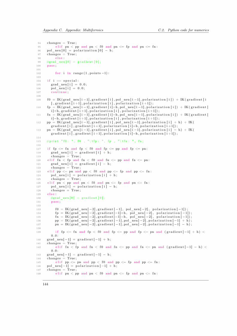
Appendix C. Appendix: Multiferroics C.2. Python code for numerics

94 changes = True ;95 e l i f pn < pp and pn < f0 and pn <= fp and pn <= fn :96 pol_neu [ 0 ] = po l a r i z a t i o n [ 0 ] − h ;97 changes = True ;98 e l s e :99 #grad_neu [ 0 ] = grad i en t [ 0 ] ;

100 pass ;101

102 f o r i in range (1 , po ints −1) :103

104 i f i == s p e c i a l :105 grad_neu [ i ] = 0 . 0 ;106 pol_neu [ i ] = 0 . 0 ;107 cont inue ;108

109 f 0 = IK( grad_neu [ i −1] , g rad i en t [ i ] , pol_neu [ i −1] , p o l a r i z a t i o n [ i ] ) + IK( grad i en t [ i] , g rad i en t [ i +1] , p o l a r i z a t i o n [ i ] , p o l a r i z a t i o n [ i +1]) ;

110 fp = IK( grad_neu [ i −1] , g rad i en t [ i ]+h , pol_neu [ i −1] , p o l a r i z a t i o n [ i ] ) + IK( grad i en t [i ]+h , g rad i en t [ i +1] , p o l a r i z a t i o n [ i ] , p o l a r i z a t i o n [ i +1]) ;

111 fn = IK( grad_neu [ i −1] , g rad i en t [ i ]−h , pol_neu [ i −1] , p o l a r i z a t i o n [ i ] ) + IK( grad i en t [i ]−h , g rad i en t [ i +1] , p o l a r i z a t i o n [ i ] , p o l a r i z a t i o n [ i +1]) ;

112 pp = IK( grad_neu [ i −1] , g rad i en t [ i ] , pol_neu [ i −1] , p o l a r i z a t i o n [ i ] + h) + IK(grad i en t [ i ] , g rad i en t [ i +1] , p o l a r i z a t i o n [ i ]+h , p o l a r i z a t i o n [ i +1]) ;

113 pn = IK( grad_neu [ i −1] , g rad i en t [ i ] , pol_neu [ i −1] , p o l a r i z a t i o n [ i ] − h) + IK(grad i en t [ i ] , g rad i en t [ i +1] , p o l a r i z a t i o n [ i ]−h , p o l a r i z a t i o n [ i +1]) ;

114

115 #pr in t " f0 : " , f 0 , "\ t fp : " , fp , "\ t fn : " , fn ;116

117 i f fp <= fn and fp < f0 and fp <= pp and fp <= pn :118 grad_neu [ i ] = grad i en t [ i ] + h ;119 changes = True ;120 e l i f fn < fp and fn < f0 and fn <= pp and fn <= pn :121 grad_neu [ i ] = grad i en t [ i ] − h ;122 changes = True ;123 e l i f pp <= pn and pp < f0 and pp <= fp and pp <= fn :124 pol_neu [ i ] = po l a r i z a t i o n [ i ] + h ;125 changes = True ;126 e l i f pn < pp and pn < f0 and pn <= fp and pn <= fn :127 pol_neu [ i ] = po l a r i z a t i o n [ i ] − h ;128 changes = True ;129 e l s e :130 #grad_neu [ 0 ] = grad i en t [ 0 ] ;131 pass ;132

133 f 0 = IK( grad_neu [−2] , g rad i en t [−1] , pol_neu [−2] , p o l a r i z a t i o n [−1]) ;134 fp = IK( grad_neu [−2] , g rad i en t [−1]+h , pol_neu [−2] , p o l a r i z a t i o n [−1]) ;135 fn = IK( grad_neu [−2] , g rad i en t [−1]−h , pol_neu [−2] , p o l a r i z a t i o n [−1]) ;136 pp = IK( grad_neu [−2] , g rad i en t [−1] , pol_neu [−2] , p o l a r i z a t i o n [−1] + h) ;137 pn = IK( grad_neu [−2] , g rad i en t [−1] , pol_neu [−2] , p o l a r i z a t i o n [−1] − h) ;138

139 i f fp <= fn and fp < f0 and fp <= pp and fp <= pn and ( g rad i en t [−1] + h) <0 . 0 :

140 grad_neu [−1] = grad i en t [−1] + h ;141 changes = True ;142 e l i f fn < fp and fn < f0 and fn <= pp and fn <= pn and ( g rad i en t [−1] − h) <

0 . 0 :143 grad_neu [−1] = grad i en t [−1] − h ;144 changes = True ;145 e l i f pp <= pn and pp < f0 and pp <= fp and pp <= fn :146 pol_neu [−1] = po l a r i z a t i o n [−1] + h ;147 changes = True ;148 e l i f pn < pp and pn < f0 and pn <= fp and pn <= fn :

144

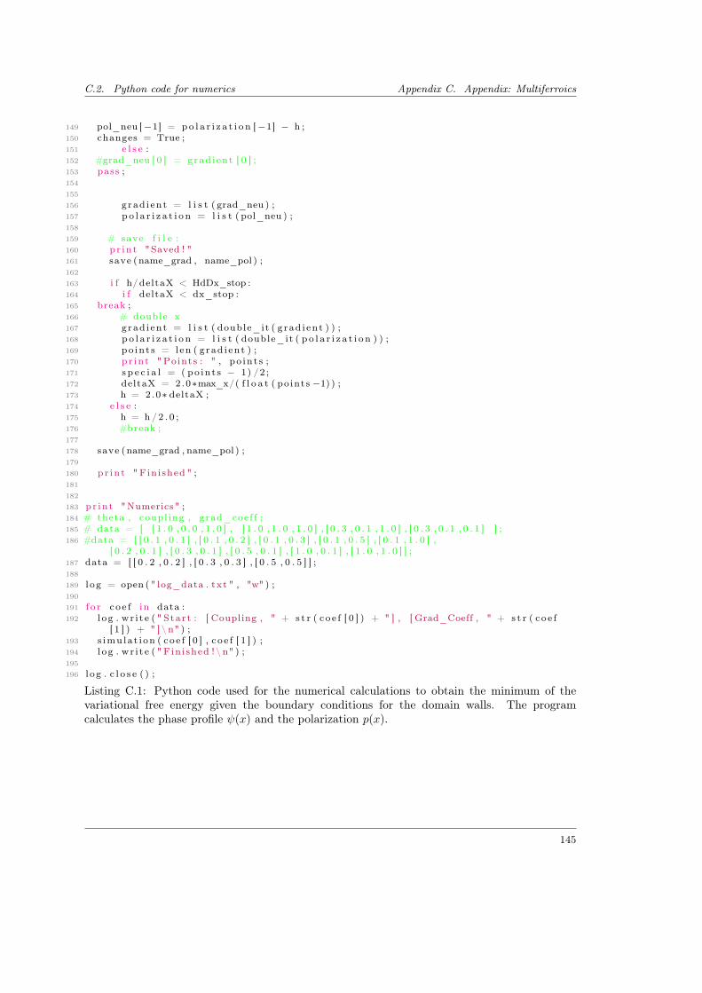
C.2. Python code for numerics Appendix C. Appendix: Multiferroics

149 pol_neu [−1] = po l a r i z a t i o n [−1] − h ;150 changes = True ;151 e l s e :152 #grad_neu [ 0 ] = grad i en t [ 0 ] ;153 pass ;154

155

156 grad i en t = l i s t ( grad_neu ) ;157 po l a r i z a t i o n = l i s t ( pol_neu ) ;158

159 # save f i l e :160 pr in t "Saved ! "161 save (name_grad , name_pol ) ;162

163 i f h/deltaX < HdDx_stop :164 i f deltaX < dx_stop :165 break ;166 # double x167 grad i en t = l i s t ( double_it ( g rad i en t ) ) ;168 po l a r i z a t i o n = l i s t ( double_it ( p o l a r i z a t i o n ) ) ;169 po in t s = len ( g rad i en t ) ;170 pr in t "Points : " , po in t s ;171 s p e c i a l = ( po in t s − 1) /2 ;172 deltaX = 2.0∗max_x/( f l o a t ( po ints −1) ) ;173 h = 2.0∗ deltaX ;174 e l s e :175 h = h /2 . 0 ;176 #break ;177

178 save (name_grad , name_pol ) ;179

180 pr in t " Fin i shed " ;181

182

183 pr in t "Numerics" ;184 # theta , coupl ing , grad_coef f ;185 # data = [ [ 1 . 0 , 0 . 0 , 1 . 0 ] , [ 1 . 0 , 1 . 0 , 1 . 0 ] , [ 0 . 3 , 0 . 1 , 1 . 0 ] , [ 0 . 3 , 0 . 1 , 0 . 1 ] ] ;186 #data = [ [ 0 . 1 , 0 . 1 ] , [ 0 . 1 , 0 . 2 ] , [ 0 . 1 , 0 . 3 ] , [ 0 . 1 , 0 . 5 ] , [ 0 . 1 , 1 . 0 ] ,

[ 0 . 2 , 0 . 1 ] , [ 0 . 3 , 0 . 1 ] , [ 0 . 5 , 0 . 1 ] , [ 1 . 0 , 0 . 1 ] , [ 1 . 0 , 1 . 0 ] ] ;187 data = [ [ 0 . 2 , 0 . 2 ] , [ 0 . 3 , 0 . 3 ] , [ 0 . 5 , 0 . 5 ] ] ;188

189 l og = open ( " log_data . txt " , "w" ) ;190

191 f o r c o e f in data :192 l og . wr i t e ( " Star t : [ Coupling , " + s t r ( c o e f [ 0 ] ) + " ] , [ Grad_Coeff , " + s t r ( c o e f

[ 1 ] ) + " ] \ n" ) ;193 s imu la t i on ( co e f [ 0 ] , c o e f [ 1 ] ) ;194 l og . wr i t e ( " Fin i shed ! \ n" ) ;195

196 l og . c l o s e ( ) ;

Listing C.1: Python code used for the numerical calculations to obtain the minimum of thevariational free energy given the boundary conditions for the domain walls. The programcalculates the phase profile ψ(x) and the polarization p(x).

145

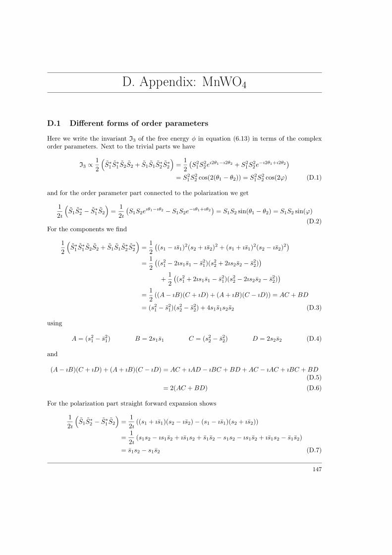
D. Appendix: MnWO4

D.1 Different forms of order parameters

Here we write the invariant I3 of the free energy φ in equation (6.13) in terms of the complexorder parameters. Next to the trivial parts we have

I3 ∝1

2

(S∗1 S

∗1 S2S2 + S1S1S

∗2 S∗2

)=

1

2

(S2

1S22eı2θ1−ı2θ2 + S2

1S22e−ı2θ1+ı2θ2

)= S2

1S22 cos(2(θ1 − θ2)) = S2

1S22 cos(2ϕ) (D.1)

and for the order parameter part connected to the polarization we get

1

2ı

(S1S

∗2 − S∗1 S2

)=

1

2ı

(S1S2e

ıθ1−ıθ2 − S1S2e−ıθ1+ıθ2

)= S1S2 sin(θ1 − θ2) = S1S2 sin(ϕ)

(D.2)For the components we find

1

2

(S∗1 S

∗1 S2S2 + S1S1S

∗2 S∗2

)=

1

2

((s1 − ıs1)2(s2 + ıs2)2 + (s1 + ıs1)2(s2 − ıs2)2

)=

1

2

((s2

1 − 2ıs1s1 − s21)(s2

2 + 2ıs2s2 − s22))

+1

2

((s2

1 + 2ıs1s1 − s21)(s2

2 − 2ıs2s2 − s22))

=1

2((A− ıB)(C + ıD) + (A+ ıB)(C − ıD)) = AC +BD

= (s21 − s2

1)(s22 − s2

2) + 4s1s1s2s2 (D.3)

using

A = (s21 − s2

1) B = 2s1s1 C = (s22 − s2

2) D = 2s2s2 (D.4)

and

(A− ıB)(C + ıD) + (A+ ıB)(C − ıD) = AC + ıAD − ıBC +BD +AC − ıAC + ıBC +BD(D.5)

= 2(AC +BD) (D.6)

For the polarization part straight forward expansion shows

1

2ı

(S1S

∗2 − S∗1 S2

)=

1

2ı((s1 + ıs1)(s2 − ıs2)− (s1 − ıs1)(s2 + ıs2))

=1

2ı(s1s2 − ıs1s2 + ıs1s2 + s1s2 − s1s2 − ıs1s2 + ıs1s2 − s1s2)

= s1s2 − s1s2 (D.7)

147

Appendix D. Appendix: MnWO4 D.2. Transition at TN : temperature fluctuations in S1

D.2 Transition at TN : temperature fluctuations in S1

Considering the phase transition at TN where α2 = a2(T − TN ) is 0. Below TN the orderparameter S2 is non-zero, and in the region T2 < T < TN : α1 > 0 and the order parameter S1 is0. Let us consider the effect of thermal fluctuations of S1 around 0 (ignoring fluctuations in S2

around its equilibrium value). Denoting the thermal average with 〈. . . 〉 we make the followingassumptions concerning the fluctuations. The order parameter fluctuates around 0

〈S1〉 = 0 ⇒ 〈s1〉 = 〈s1〉 = 0 (D.8)

the fluctuations for the different components s1 and s1 are uncorrelated

〈f(s1)g(s1)〉 = 〈f(s1)〉〈g(s1)〉 (D.9)

and the two components fluctuate according to the same distribution, meaning their momentsare identical

〈sn1 〉 = 〈s1n〉 ∀n ∈ N (D.10)

Averaging over the free energy Φ we get

〈Φ〉 = Φ0(T )− f(T ) +α2

2(s2

2 + s22) +

β2

4(s2

2 + s22)2 + α1〈s2

1〉+β1

4〈(s2

1 + s21)2〉︸ ︷︷ ︸

≡g(T )

(D.11)

+γ1

2

((s2

2 − s22)(〈s2

1〉 − 〈s21〉) + 4s2s2〈s1s1〉

)︸ ︷︷ ︸

=0

+γ2

4

⟨((s2

2 − s22)(s2

1 − s21) + 4s2s2s1s1

)2⟩︸ ︷︷ ︸=A

(D.12)

− 1

2δ2ε0yy

⟨(s1s2 − s1s2)2

⟩︸ ︷︷ ︸=〈s21〉(s22+s22)

(D.13)

The contribution A from the coupling γ2 can be written as

A =γ2

4

((s2

2 − s22)2(〈s4

1〉 − 2〈s21s

21〉+ 〈s4

1〉) + 16s22s

22〈s2

1s21〉)

=γ2

2

((s2

2 − s22)2(〈s4

1〉 − 〈s21〉2) + 8s2

2s22〈s2

1〉2)

(D.14)

=γ2

2

((s4

2 − 2s22s

22 + s2

2)(〈s41〉 − 〈s2

1〉2) + 8s22s

22〈s2

1〉2)

(D.15)

=γ2

2

((s2

2 + s22)2(〈s4

1〉 − 〈s21〉2)− 4s2

2s22(〈s4

1〉 − 〈s21〉2) + 8s2

2s22〈s2

1〉2)

(D.16)

=γ′24

(s22 + s2

2)2 + ζs22s

22 (D.17)

with

γ′2 = 2γ2(〈s41〉 − 〈s2

1〉2) ζ = 4γ2

(3〈s2

1〉2 − 〈s41〉)

(D.18)

The changes to the free energy due to the fluctuations in S2 are therefor

φ0(T )→ φ′0(T ) = φ0(T ) + g(T ) (D.19)

α2 → α′2 = α2 − δ2ε0yy〈s21〉 (D.20)

β2 → β′2 = β2 + 2γ2(〈s41〉 − 〈s2

1〉2) (D.21)

ζ → 4γ2

(3〈s2

1〉2 − 〈s41〉)

(D.22)

148

D.2. Transition at TN : temperature fluctuations in S1 Appendix D. Appendix: MnWO4

With the new free energy

〈Φ〉 = Φ′0(T )− f(T ) +α′22

(s22 + s2

2) +β′24

(s22 + s2

2)2 + ζs22s

22 (D.23)

The system can also be brought of the form of a N -component model with cubic anisotropy(N = 2)

〈Φ〉 = g(T ) +m2

0

2

N∑i=1

φ2i +

u0

4!

(N∑i=1

φ2i

)2

+v0

4!

N∑i=1

(φ2i )

2 (D.24)

with φ1 = s2, ϕ2 = s2 and

m20 = α′2 = α2 − δ2ε0yy〈s2

1〉 u0 = 6β′2 + 6γ′2(1 +ζ

2) v0 = −3ζγ′2 (D.25)

For spacial varying order parameters in d dimensions (here d = 3) the system is described by

H =

∫ddx

1

2

N∑i=1

(m2

0φ2i + (∇φi)

2)

+u0

4!

(N∑i=1

φ2i

)2

+v0

4!

N∑i=1

(φ2i )

2

(D.26)

This model has been studied in ε = 4 − d expansion and the stable fix point of the systemcorresponds to the O(N) symmetrical Heisenberg fix point.

Gaussian fluctuations: In the special case of Gaussian fluctuations we can use Wicks theorem

〈s41〉 = 3〈s2

1〉2 (D.27)

which leads toζ = 0 ⇒ v0 = 0 (D.28)

a vanishing anisotropy term. The model is then identical to the O(2) model and the transitionobviously in the 3D-XY universality class with the symmetric fixpoint being the stable one.

Mean-Field In the framework of the mean field study, the invariant corresponding to γ2 is ofO(S8) and is not playing an important role stabilizing the phases. Since the anisotropy vanishesfor γ2 = 0 (ignoring said term in the Landau-expansion) it should not play an important role.

Non-Gaussian fluctuations In the case of non-Gaussian fluctuations and including the effectof γ2, we get a ζ 6= 0 and therefor an anisotropic term in the O(2) model. This model has beenstudied by and for a critical N < Nc it has been found that the symmetric Heisenberg-fixpointis still the stable fixpoint for the system. There is still some debate on the exact value of Nc ford = 3, [107], which is in the order of Nc ∼ 3, however calculations by Aharony, [108, 109] andBrézin et al. [110] show that for N = 2 in d = 3 the symmetric fix point is the stable one. Thetransition is then in the O(2)-symmetric universality class. The exponents up to O(ε5) and adiscussion on the stability of the Heisenberg fix point in the presents of cubic anisotropy is givenin [91], here we will only use the exponents up to O(ε3) being

η =N + 2

2(N + 8)2ε2 ν−1 = 2− N + 2

N + 8ε− N + 2

2(N + 8)3(13N + 44)ε2 (D.29)

=1

50=

73

50(D.30)

149

Appendix D. Appendix: MnWO4 D.3. Transition at T2: Frozen S1 order parameter

where the numerical values are calculated for N = 2 and ε = 1. Using the hyperscaling relations,we can compute the missing exponents

α = 2− νd β =ν

2(d− 2 + η) γ = ν(2− η) δ =

d+ 2− ηd− 2 + η

(D.31)

= − 4

73≈ −0.055 =

51

146≈ 0.349 =

99

73≈ 1.356 =

83

17≈ 4.882 (D.32)

Being the exponents of the 3D-XY (O(2)) universality class.

D.3 Transition at T2: Frozen S1 order parameter

For T < TN we have α2 < 0 and the field in S2 has reached a non-zero value. Approaching T2

where α1(T2) = 0, the field in S1 will be critical. Compared to the fluctuations in S1 the field inS2 can be considered as frozen in first order. The values for s2 and s2 can therefor be replacedby their equilibrium values se2 = 〈s2〉 and se2 = 〈s2〉. The theory left is only dependent on s1, s1

and the polarization Py, which are coupled through bi-linear terms ∼ s1s1, ∼ Pys1 and ∼ Py s1.For a cleaner notation in the following section we switch se2 → s2 and se2 → s2. The free energyaround T0 under these considerations can be written as

Φ = g(T ) +α1

2(s2

1 + s21) +

β1

4(s2

1 + s21)2 +

1

2ε0yyP 2y (D.33)

+γ1

2

((s2

2 − s22)(s2

1 − s21) + 4s1s1s2s2

)+γ2

4

((s2

1 − s21)(s2

2 − s22) + 4s1s1s2s2

)2 (D.34)

+ δPy(s1s2 − s1s2) (D.35)

Introducing the vector p = (s1, s1, Py), the quadratic an bi-linear terms can be written as

ΦM =1

2pT M p (D.36)

with the matrix M given in equation (6.25). We can know rotate the system in its diagonal formin order to eliminate the bi-linear fields. The equilibrium case for the frozen out components s2

and s2 is symmetric in the phase θ2 and can be written as

s2 = s cos(θ2) s2 = s sin(θ2) s =

√−α′2β′2

(D.37)

where θ2 is arbitrary. With cos2(θ2) − sin2(θ2) = cos(2θ2) and cos(θ2) sin(θ2) = 12 sin(θ2) the

matrix M can be simlified.

No coupling to polarization (δ = 0): In the simple case of no coupling to the polarizationPy we have the following characteristic polynomial for the eigenvalues λ

(α1 + γ1s2 cos(2θ2)− λ)(α1 − γ1s

2 cos(2θ2)− λ)(1

ε0yy− λ)− γ2

1s4 sin2(2θ2)(

1

ε0yy− λ) = 0 (D.38)

with λ3 = 1ε0yy

and

λ2 − 2α1λ+ α21 − γ2

1s4 = 0 (D.39)

150

D.3. Transition at T2: Frozen S1 order parameter Appendix D. Appendix: MnWO4

givingλ1/2 = α1 ± γ1s

2 (D.40)

So already in the absence of a coupling via the polarization the two components become criticalat different temperatures. Calculating the eigenvectors corresponding to the eigenvalues we easilyfind

λ3 =1

ε0yy⇒ v3 =

0

0

1

(D.41)

For λ1 we find from Mv1 = λ1v1 with v1 = (x, y, z) the following equations

cos(2θ2)x+ sin(2θ2)y = −x (D.42)sin(2θ2)x− cos(2θ2)x = −y (D.43)

1

ε0yyz = (α1 − γ1s

2)z (D.44)

with this we find z = 0 and the first two equations are identical and result in

cos(θ2)x+ sin(θ2)y = 0 (D.45)

which leads to the solution

λ1 = α1 − γ1s2 ⇒ v1 =

− sin(θ2)

cos(θ2)

0

(D.46)

and orthogonal to this (or by directly solving for λ3) we find

λ2 = α1 + γ1s2 ⇒ v2 =

cos(θ2)

sin(θ2)

0

(D.47)

From the eigenvectors we can construct the rotation matrix R

R =

− sin(θ2) cos(θ2) 0

cos(θ2) sin(θ2) 0

0 0 1

(D.48)

and introduce the new fields

u =

u1

u2

u3

= Rp =

−s1 sin(θ2) + s1 cos(θ2)

s1 cos(θ2) + s1 sin(θ2)

Py

(D.49)

so that

(Rp)T (R ·M(δ = 0) ·RT )(Rp) ⇒ uT

λ1 0 0

0 λ2 0

0 0 λ2

u (D.50)

When u1 becomes critical the equilibrium-values are

u1 = c u2 = 0 u3 = 0 (D.51)

151

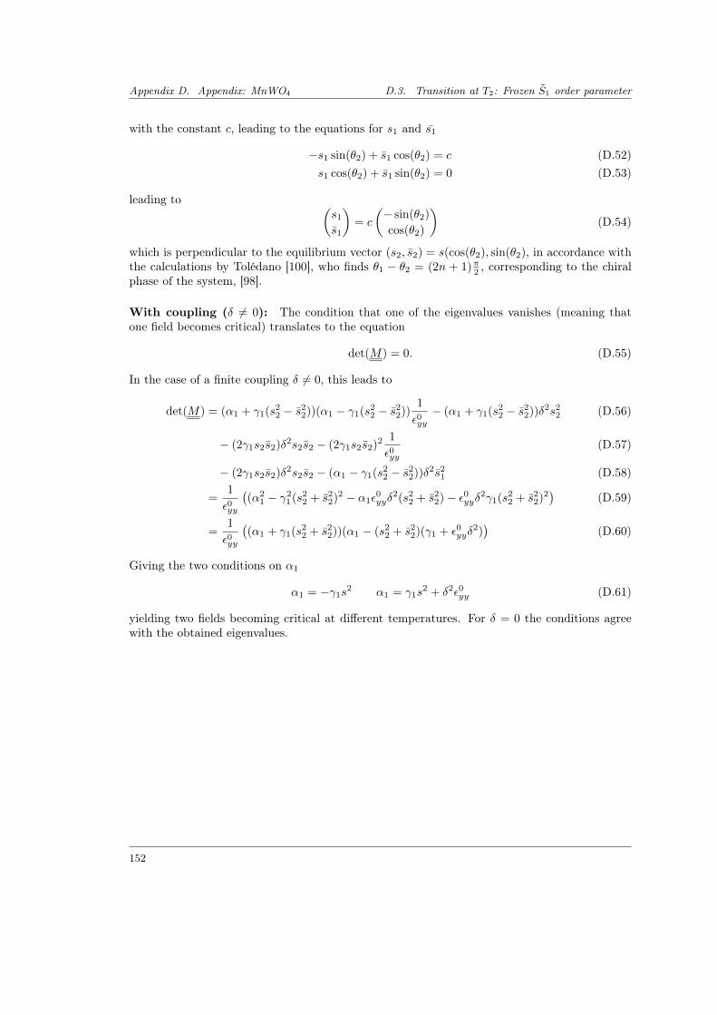
Appendix D. Appendix: MnWO4 D.3. Transition at T2: Frozen S1 order parameter

with the constant c, leading to the equations for s1 and s1

−s1 sin(θ2) + s1 cos(θ2) = c (D.52)s1 cos(θ2) + s1 sin(θ2) = 0 (D.53)

leading to (s1

s1

)= c

(− sin(θ2)

cos(θ2)

)(D.54)

which is perpendicular to the equilibrium vector (s2, s2) = s(cos(θ2), sin(θ2), in accordance withthe calculations by Tolédano [100], who finds θ1 − θ2 = (2n + 1)π2 , corresponding to the chiralphase of the system, [98].

With coupling (δ 6= 0): The condition that one of the eigenvalues vanishes (meaning thatone field becomes critical) translates to the equation

det(M) = 0. (D.55)

In the case of a finite coupling δ 6= 0, this leads to

det(M) = (α1 + γ1(s22 − s2

2))(α1 − γ1(s22 − s2

2))1

ε0yy− (α1 + γ1(s2

2 − s22))δ2s2

2 (D.56)

− (2γ1s2s2)δ2s2s2 − (2γ1s2s2)2 1

ε0yy(D.57)

− (2γ1s2s2)δ2s2s2 − (α1 − γ1(s22 − s2

2))δ2s21 (D.58)

=1

ε0yy

((α2

1 − γ21(s2

2 + s22)2 − α1ε

0yyδ

2(s22 + s2

2)− ε0yyδ2γ1(s22 + s2

2)2)

(D.59)

=1

ε0yy

((α1 + γ1(s2

2 + s22))(α1 − (s2

2 + s22)(γ1 + ε0yyδ

2))

(D.60)

Giving the two conditions on α1

α1 = −γ1s2 α1 = γ1s

2 + δ2ε0yy (D.61)

yielding two fields becoming critical at different temperatures. For δ = 0 the conditions agreewith the obtained eigenvalues.

152

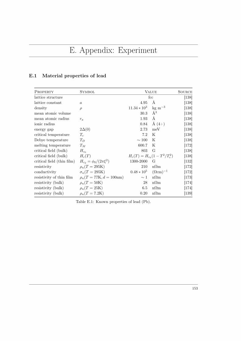
E. Appendix: Experiment

E.1 Material properties of lead

Property Symbol Value Sourcelattice structure fcc [138]lattice constant a 4.95 Å [138]density ρ 11.34 ∗ 103 kg m−3 [138]mean atomic volume 30.3 Å3 [138]mean atomic radius ra 1.93 Å [138]ionic radius 0.84 Å (4+) [138]energy gap 2∆(0) 2.73 meV [138]critical temperature Tc 7.2 K [138]Debye temperature TD ∼ 100 K [138]melting temperature TM 600.7 K [172]critical field (bulk) Hc0 803 G [138]critical field (bulk) Hc(T ) Hc(T ) = Hc0(1− T 2/T 2

c ) [138]critical field (thin film) Hc2 = φ0/(2πξ

2) 1300-2000 G [132]resistivity ρn(T = 295K) 210 nΩm [172]conductivity σn(T = 295K) 0.48 ∗ 105 (Ωcm)−1 [172]resistivity of thin film ρn(T = 77K, d = 100nm) ∼ 1 nΩm [173]resistivity (bulk) ρn(T = 50K) 28 nΩm [174]resistivity (bulk) ρn(T = 25K) 6.5 nΩm [174]resistivity (bulk) ρn(T = 7.2K) 0.20 nΩm [139]

Table E.1: Known properties of lead (Pb).

153

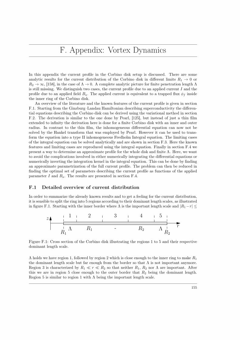
F. Appendix: Vortex Dynamics

In this appendix the current profile in the Corbino disk setup is discussed. There are someanalytic results for the current distribution of the Corbino disk in different limits R1 → 0 orR2 →∞, [158], in the case of Λ→ 0. A complete analytic picture for finite penetration length Λis still missing. We distinguish two cases, the current profile due to an applied current I and theprofile due to an applied field Ba. The applied current is equivalent to a trapped flux φf insidethe inner ring of the Corbino disk.

An overview of the literature and the known features of the current profile is given in sectionF.1. Starting from the Ginzburg–Landau Hamiltonian describing superconductivity the differen-tial equations describing the Corbino disk can be derived using the variational method in sectionF.2. The derivation is similar to the one done by Pearl, [125], but instead of just a thin filmextended to infinity the derivation here is done for a finite Corbino disk with an inner and outerradius. In contrast to the thin film, the inhomogeneous differential equation can now not besolved by the Hankel transform that was employed by Pearl. However it can be used to trans-form the equation into a type II inhomogeneous Fredholm Integral equation. The limiting casesof the integral equation can be solved analytically and are shown in section F.3. Here the knownfeatures and limiting cases are reproduced using the integral equation. Finally in section F.4 wepresent a way to determine an approximate profile for the whole disk and finite Λ. Here, we wantto avoid the complications involved in either numerically integrating the differential equations ornumerically inverting the integration kernel in the integral equation. This can be done by findingan approximate parametrization of the full current profile. The problem can then be reduced infinding the optimal set of parameters describing the current profile as functions of the appliedparameter I and Ba. The results are presented in section F.4.

F.1 Detailed overview of current distribution

In order to summarize the already known results and to get a feeling for the current distribution,it is sensible to split the ring into 5 regions according to their dominant length scales, as illustratedin figure F.1. Starting with the inner border where Λ is the important length scale and |R1−r| ≤

z

rR1 R2

1

Λ

2

R1

3

-

4

R2

5

Λ

Figure F.1: Cross section of the Corbino disk illustrating the regions 1 to 5 and their respectivedominant length scale.

Λ holds we have region 1, followed by region 2 which is close enough to the inner ring to make R1

the dominant length scale but far enough from the border so that Λ is not important anymore.Region 3 is characterized by R1 r R2 so that neither R1, R2 nor Λ are important. Afterthis we are in region 5 close enough to the outer border that R2 being the dominant length.Region 5 is similar to region 1 with Λ being the important length scale.

155

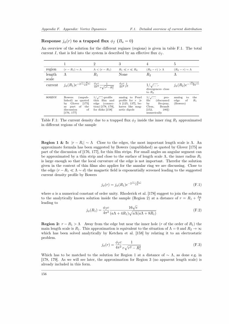
Appendix F. Appendix: Vortex Dynamics F.1. Detailed overview of current distribution

Response jφ(r) to a trapped flux φf (Ba = 0)

An overview of the solution for the different regimes (regions) is given in table F.1. The totalcurrent I, that is fed into the system is described by an effective flux φf .

1 2 3 4 5region (r − R1) ∼ Λ Λ < (r − R1) R1 r R2 (R2 − r) > Λ (R2 − r) ∼ Λ

lengthscale

Λ R1 None R2 Λ

current jφ(R1)e−2(r−R1)aΛ

φf c4π2

1

r√r2−R2

1

φf c4π2

1r2 1/

√. . .-

divergences closeto R2

jφ(R2)e−(R2−x)bΛ

source Bowers (unpub-lished) as quotedby Glover [175]as part of thediscussion of[176, 177]

1/√. . .-profile

thin film andedge (connec-tion) [178, 179],for disks [158]

analog to Pearlprofile for r Λ [125, 137], be-haves like mag-netic dipole

1/√. . . pro-

file (discussedby Brojeny,Clem, Brandt[152, 180])numerically

analog to theedge of R1

(Bowers)

Table F.1: The current density due to a trapped flux φf inside the inner ring R1 approximatedin different regions of the sample

Region 1 & 5: |r − Ri| ∼ Λ Close to the edges, the most important length scale is Λ. Anapproximate formula has been suggested by Bowers (unpublished) as quoted by Glover [175] aspart of the discussion of [176, 177], for thin film strips. For small angles an angular segment canbe approximated by a thin strip and close to the surface of length scale Λ, the inner radius R1

is large enough so that the local curvature of the edge is not important. Therefor the solutiongiven in the context of thin films also applies for the annular ring we are discussing. Close tothe edge (r−R1 Λ ∼ d) the magnetic field is exponentially screened leading to the suggestedcurrent density profile by Bowers

jφ(r) = jφ(R1)e−2(r−R1)aΛ (F.1)

where a is a numerical constant of order unity. Rhoderick et al. [178] suggest to join the solutionto the analytically known solution inside the sample (Region 2) at a distance of r = R1 + Λa

4leading to

jφ(R1) =φfc

4π2

16√e

(aΛ + 4R1)√aΛ(aΛ + 8R1)

(F.2)

Region 2: r −R1 > Λ Away from the edge but near the inner hole (r of the order of R1) themain length scale is R1. This approximation is equivalent to the situation of Λ = 0 and R2 →∞which has been solved analytically by Ketchen et al. [158] by relating it to an electrostaticproblem.

jφ(r) =φfc

4π2

1

r√r2 −R2

1

(F.3)

Which has to be matched to the solution for Region 1 at a distance of ∼ Λ, as done e.g. in[178, 179]. As we will see later, the approximation for Region 3 (no apparent length scale) isalready included in this form.

156

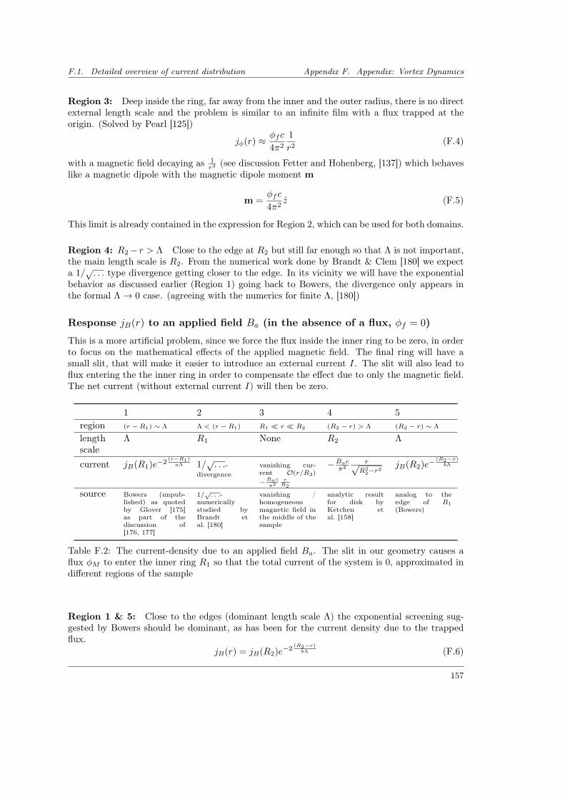
F.1. Detailed overview of current distribution Appendix F. Appendix: Vortex Dynamics

Region 3: Deep inside the ring, far away from the inner and the outer radius, there is no directexternal length scale and the problem is similar to an infinite film with a flux trapped at theorigin. (Solved by Pearl [125])

jφ(r) ≈ φfc

4π2

1

r2(F.4)

with a magnetic field decaying as 1r3 (see discussion Fetter and Hohenberg, [137]) which behaves

like a magnetic dipole with the magnetic dipole moment m

m =φfc

4π2z (F.5)

This limit is already contained in the expression for Region 2, which can be used for both domains.

Region 4: R2− r > Λ Close to the edge at R2 but still far enough so that Λ is not important,the main length scale is R2. From the numerical work done by Brandt & Clem [180] we expecta 1/√. . . type divergence getting closer to the edge. In its vicinity we will have the exponential

behavior as discussed earlier (Region 1) going back to Bowers, the divergence only appears inthe formal Λ→ 0 case. (agreeing with the numerics for finite Λ, [180])

Response jB(r) to an applied field Ba (in the absence of a flux, φf = 0)

This is a more artificial problem, since we force the flux inside the inner ring to be zero, in orderto focus on the mathematical effects of the applied magnetic field. The final ring will have asmall slit, that will make it easier to introduce an external current I. The slit will also lead toflux entering the the inner ring in order to compensate the effect due to only the magnetic field.The net current (without external current I) will then be zero.

1 2 3 4 5region (r − R1) ∼ Λ Λ < (r − R1) R1 r R2 (R2 − r) > Λ (R2 − r) ∼ Λ

lengthscale

Λ R1 None R2 Λ

current jB(R1)e−2(r−R1)aΛ 1/

√. . .-

divergencevanishing cur-rent O(r/R2)

−Bacπ2

rR2

−Bacπ2r√

R22−r2

jB(R2)e−(R2−x)bΛ

source Bowers (unpub-lished) as quotedby Glover [175]as part of thediscussion of[176, 177]

1/√. . .-

numericallystudied byBrandt etal. [180]

vanishing /homogeneousmagnetic field inthe middle of thesample

analytic resultfor disk byKetchen etal. [158]

analog to theedge of R1

(Bowers)

Table F.2: The current-density due to an applied field Ba. The slit in our geometry causes aflux φM to enter the inner ring R1 so that the total current of the system is 0, approximated indifferent regions of the sample

Region 1 & 5: Close to the edges (dominant length scale Λ) the exponential screening sug-gested by Bowers should be dominant, as has been for the current density due to the trappedflux.

jB(r) = jB(R2)e−2(R2−r)bΛ (F.6)

157

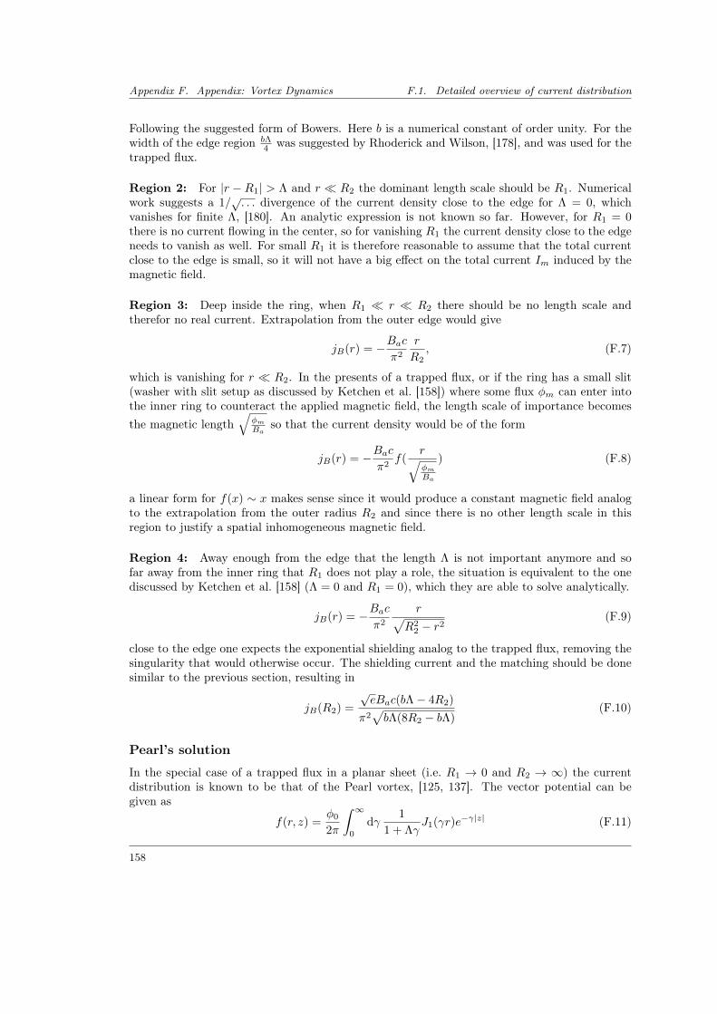
Appendix F. Appendix: Vortex Dynamics F.1. Detailed overview of current distribution

Following the suggested form of Bowers. Here b is a numerical constant of order unity. For thewidth of the edge region bΛ

4 was suggested by Rhoderick and Wilson, [178], and was used for thetrapped flux.

Region 2: For |r − R1| > Λ and r R2 the dominant length scale should be R1. Numericalwork suggests a 1/

√. . . divergence of the current density close to the edge for Λ = 0, which

vanishes for finite Λ, [180]. An analytic expression is not known so far. However, for R1 = 0there is no current flowing in the center, so for vanishing R1 the current density close to the edgeneeds to vanish as well. For small R1 it is therefore reasonable to assume that the total currentclose to the edge is small, so it will not have a big effect on the total current Im induced by themagnetic field.

Region 3: Deep inside the ring, when R1 r R2 there should be no length scale andtherefor no real current. Extrapolation from the outer edge would give

jB(r) = −Bacπ2

r

R2, (F.7)

which is vanishing for r R2. In the presents of a trapped flux, or if the ring has a small slit(washer with slit setup as discussed by Ketchen et al. [158]) where some flux φm can enter intothe inner ring to counteract the applied magnetic field, the length scale of importance becomesthe magnetic length

√φmBa

so that the current density would be of the form

jB(r) = −Bacπ2

f(r√φmBa

) (F.8)

a linear form for f(x) ∼ x makes sense since it would produce a constant magnetic field analogto the extrapolation from the outer radius R2 and since there is no other length scale in thisregion to justify a spatial inhomogeneous magnetic field.

Region 4: Away enough from the edge that the length Λ is not important anymore and sofar away from the inner ring that R1 does not play a role, the situation is equivalent to the onediscussed by Ketchen et al. [158] (Λ = 0 and R1 = 0), which they are able to solve analytically.

jB(r) = −Bacπ2

r√R2

2 − r2(F.9)

close to the edge one expects the exponential shielding analog to the trapped flux, removing thesingularity that would otherwise occur. The shielding current and the matching should be donesimilar to the previous section, resulting in

jB(R2) =

√eBac(bΛ− 4R2)

π2√bΛ(8R2 − bΛ)

(F.10)

Pearl’s solution

In the special case of a trapped flux in a planar sheet (i.e. R1 → 0 and R2 → ∞) the currentdistribution is known to be that of the Pearl vortex, [125, 137]. The vector potential can begiven as

f(r, z) =φ0

2π

∫ ∞0

dγ1

1 + ΛγJ1(γr)e−γ|z| (F.11)

158

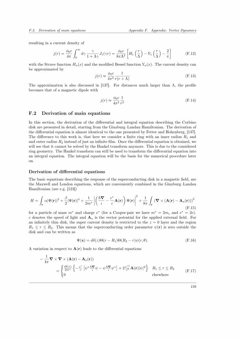
F.2. Derivation of main equations Appendix F. Appendix: Vortex Dynamics

resulting in a current density of

j(r) =φ0c

4π

∫ ∞0

dγγ

1 + ΛγJ1(γr) =

φ0c

8πΛ2

[H1

( rΛ

)− Y1

( rΛ

)− 2

π

](F.12)

with the Struve function Hn(x) and the modified Bessel function Yn(x). The current density canbe approximated by

j(r) ≈ φ0c

4π2

1

r(r + Λ)(F.13)

The approximation is also discussed in [137]. For distances much larger than Λ, the profilebecomes that of a magnetic dipole with

j(r) ≈ φ0c

4π2

1

r2(F.14)

F.2 Derivation of main equations

In this section, the derivation of the differential and integral equation describing the Corbinodisk are presented in detail, starting from the Ginzburg–Landau Hamiltonian. The derivation ofthe differential equation is almost identical to the one presented by Fetter and Hohenberg, [137].The difference to this work is, that here we consider a finite ring with an inner radius R1 andand outer radius R2 instead of just an infinite film. Once the differential equation is obtained, wewill see that it cannot be solved by the Hankel transform anymore. This is due to the consideredring geometry. The Hankel transform can still be used to transform the differential equation intoan integral equation. The integral equation will be the basis for the numerical procedure lateron.

Derivation of differential equations

The basic equations describing the response of the superconducting disk in a magnetic field, arethe Maxwell and London equations, which are conveniently combined in the Ginzburg–LandauHamiltonian (see e.g. [123])

H =

∫r

α|Ψ(r)|2 +β

2|Ψ(r)|4 +

1

2m∗

∣∣∣∣(~∇ı− e∗

cA(r)

)Ψ(r)

∣∣∣∣2 +1

8π

∫r

(∇× (A(r)−Aa(r)))2

(F.15)for a particle of mass m∗ and charge e∗ (for a Cooper-pair we have m∗ = 2me and e∗ = 2e).c denotes the speed of light and Aa is the vector potential for the applied external field. Foran infinitely thin disk, the super current density is restricted to the z = 0 layer and the regionR1 ≤ r ≤ R2. This means that the superconducting order parameter ψ(r) is zero outside thedisk and can be written as

Ψ(x) = dδ(z)Θ(r −R1)Θ(R2 − r)ψ(r, θ). (F.16)

A variation in respect to A(r) leads to the differential equations

− 1

4π∇×∇× (A(r)−Aa(r))

=

dδ(z)2m∗

− e∗c

[ψ∗ ~∇ı ψ − ψ ~∇

ı ψ∗]+ 2 e

∗2

c2 A(r)|ψ|2

R1 ≤ r ≤ R2

0 elsewhere(F.17)

159

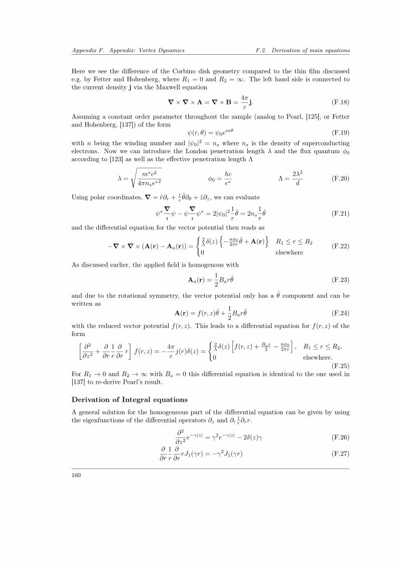
Appendix F. Appendix: Vortex Dynamics F.2. Derivation of main equations

Here we see the difference of the Corbino disk geometry compared to the thin film discussede.g. by Fetter and Hohenberg, where R1 = 0 and R2 = ∞. The left hand side is connected tothe current density j via the Maxwell equation

∇×∇×A = ∇×B =4π

cj. (F.18)

Assuming a constant order parameter throughout the sample (analog to Pearl, [125], or Fetterand Hohenberg, [137]) of the form

ψ(r, θ) = ψ0eınθ (F.19)

with n being the winding number and |ψ0|2 = ns where ns is the density of superconductingelectrons. Now we can introduce the London penetration length λ and the flux quantum φ0

according to [123] as well as the effective penetration length Λ

λ =

√m∗c2

4πnse∗2 φ0 =

hc

e∗Λ =

2λ2

d(F.20)

Using polar coordinates, ∇ = r∂r + 1r θ∂θ + z∂z, we can evaluate

ψ∗∇ıψ − ψ∇

ıψ∗ = 2|ψ0|2

1

rθ = 2ns

1

rθ (F.21)

and the differential equation for the vector potential then reads as

−∇×∇× (A(r)−Aa(r)) =

2Λδ(z)

−nφ0

2πr θ + A(r)

R1 ≤ r ≤ R2

0 elsewhere(F.22)

As discussed earlier, the applied field is homogenous with

Aa(r) =1

2Barθ (F.23)

and due to the rotational symmetry, the vector potential only has a θ component and can bewritten as

A(r) = f(r, z)θ +1

2Barθ (F.24)

with the reduced vector potential f(r, z). This leads to a differential equation for f(r, z) of theform[

∂2

∂z2+

∂

∂r

1

r

∂

∂rr

]f(r, z) = −4π

cj(r)δ(z) =

2Λδ(z)

[f(r, z) + Bar

2 −nφ0

2πr

], R1 ≤ r ≤ R2,

0 elsewhere.(F.25)

For R1 → 0 and R2 → ∞ with Ba = 0 this differential equation is identical to the one used in[137] to re-derive Pearl’s result.

Derivation of Integral equations

A general solution for the homogeneous part of the differential equation can be given by usingthe eigenfunctions of the differential operators ∂z and ∂r 1

r∂rr.

∂2

∂z2e−γ|z| = γ2e−γ|z| − 2δ(z)γ (F.26)

∂

∂r

1

r

∂

∂rrJ1(γr) = −γ2J1(γr) (F.27)

160

F.2. Derivation of main equations Appendix F. Appendix: Vortex Dynamics

From this it can be easily seen that for z > 0 the function J1(γr)e−γ|z| solves the homogeneouspart of the differential equation for every γ. This is the basis for the ansatz used by Pearl, [125],

f(r, z) =

∫ ∞0

dγg(γ)J1(γr)e−γ|z| (F.28)

which reduces the vector potential f(r, z) to the unknown function g(γ). After plugging theansatz in, the differential equation reduces to

−Λ

∫ ∞0

dγ γg(γ)J1(γr) = Θ(r −R1)Θ(R2 − r)[∫ ∞

0

dγg(γ)J1(γr) +Bar

2− φf

2πr

](F.29)

Now using the orthogonal relation of the Bessel functions∫ ∞0

dtJν(xt)tJν(yt) =1

xδ(x− y) (F.30)

we can properly transform the equation into an integral equation for g(γ) by applying∫ ∞0

dr rJ1(rη)(. . . ) (F.31)

to both sides. This transformation is also known as Hankel transform, with the interestingfeature of being its own inverse, a fact we will use later. Applying the Hankel transform resultsin

−Λg(η) =Ba2

∫ R2

R1

dr r2J1(rη)− φf2π

∫ R2

R1

drJ1(rη) +

∫ ∞0

dγ

∫ R2

R1

dr rg(γ)J1(γr)J1(rη).

(F.32)

Unlike the case discussed by Fetter and Hohenberg where R1 = 0 and R2 = ∞, the integralswith finite limits are not easy to handle. The kernel of the last integral can be brought into anicer from by splitting the integral into the 2 parts∫ R2

R1

= −∫ R1

0

+

∫ R2

0

(F.33)

Now the integral equation in its full form can be written as

Λg(η) = hφ(η)− hB(η) +

∫ ∞0

dγg(γ) K1(γ, η)−K2(γ, η) (F.34)

hφ(η) =φf2π

∫ R2

R1

dr J1(rη) =φf2π

1

η(J0(R1η)− J0(R2η)) (F.35)

hB(η) =Ba2

∫ R2

R1

dr r2J1(ηr) =Ba2

1

η

(−R2

1J2(R1η) +R22J2(R2η)

)(F.36)

K1/2(γ, η) =

∫ R1/2

0

dr J1(γr)rJ1(ηr) (F.37)

=R1/2

γ2 − η2

ηJ0(R1/2η)J1(R1/2γ)− γJ0(R1/2γ)J1(R1/2η)

(F.38)

which is a type II inhomogeneous Fredholm Integral equation. Since the equation is linear,we can split the inhomogeneous part and treat the two functions hφ(η) and hB(η) separately,

161

Appendix F. Appendix: Vortex Dynamics F.3. Limiting cases and solutions to integral equations

being equivalent to calculating the different contributions jφ(r) and jB(r). Using the Pearl ansatzon the left hand side of equation (11.8), we can relate the current density j(r) and the functiong(γ) via

j(r) =c

2π

∫ ∞0

dγ γg(γ)J1(γr) (F.39)

F.3 Limiting cases and solutions to integral equations

Using the derived integral equations for g(γ) we can look at different scenarios and solve differentlimiting cases. We will split the discussion again into the response to the trapped flux φf andthe response to the magnetic field Ba.

Equation for the trapped flux φf

Limit R2 →∞ Let us start with the special case of R2 →∞, a thin sheet with a hole of radiusR1, in which case the integration Kernel K2(η, γ) and the inhomogeneous part hφ(η) simplify to

limR2→∞

K2(η, γ) =1

ηδ(η − γ) (F.40)

limR2→∞

hφ(η) =φf2π

J0(R1η)

η(F.41)

The equation for g(η) can then be written as

g(η) =φf2π

J0(R1η)

1 + Λη+

η

1 + Λη

∫ ∞0

dγ g(γ)K1(γ, η) (F.42)

for R1 → 0 we have K1(γ, η) → 0 and J0(0) = 1, leading to Pearl’s solution of g(γ) =φf2π

11+Λγ .

To compute the Λ→ 0 limit to compare to already obtained analytic results, it turns out to bequite useful to employ a Hankel transform once more, this time with the J0(x) basis, introducing

g(η) =

∫ ∞0

dxh(x)J0(xη) (F.43)

substituting g(η) in equation (F.42)∫ ∞0

dxh(x)J0(ηx) =φf2π

J0(R1η)

1 + Λη+

η

1 + Λη

∫ ∞0

dγ

∫ ∞0

dxh(x)K1(γ, η)J0(γx) (F.44)

and using ∫ ∞0

dγ J0(xγ)K1(γ, η) =

∫ ∞0

dγ

∫ R1

0

drJ0(xγ)rJ1(rγ)J1(rη) (F.45)∫ ∞0

dγ J0(xγ)J1(rγ) =

1r r > x

0 r ≤ x (F.46)

∫ R1

x

J1(rη) =1

η(J0(xη)− J0(R1η)) Θ(a− x) (F.47)

leaves us with∫ ∞0

dxh(x)J0(ηx) =φf2π

J0(R1η)

1 + Λη+

1

1 + Λη

∫ R1

0

dxh(x) J0(xη)− J0(R1η) (F.48)

162

F.3. Limiting cases and solutions to integral equations Appendix F. Appendix: Vortex Dynamics

Now we will use the orthogonality of the Bessel functions. Applying∫∞

0dηηJ0(ηx)(. . . ) to both

sides we get

h(x) =φf2πxk(R1, x)− xk(R1, x)

∫ R1

0

dηh(η) + x

∫ R1

0

dη h(η)k(η, x) (F.49)

where we introduced

k(x, y) =

∫ ∞0

dηJ0(xη)ηJ0(yη)

1 + Λη(F.50)

as a test, we can check the R1 → 0 limit again, in which this equation reduces to Pearls result(as it should). For Λ→ 0 we find

limΛ→0

k(x, y) =1

xδ(x− y) (F.51)

resulting in a h(x) = 0 for x > R1 and for x ≤ R1∫ R1

0

dxh(x) =φf2π

(F.52)

This integral equation for h(x) has the following non–trivial solution of

h(x) =φf2π

x

R1

√R2

1 − x2Θ(R1 − x) (F.53)

Now we can compute g(γ) via the inverse Hankel transform, which evaluates to

g(γ) =

∫ ∞0

dxh(x)J0(xγ) =φf2π

sin(R1γ)

R1γ=φf2πj0(R1γ) (F.54)

where j0(x) is the spherical Bessel function. Using the relation between g(γ) and the currentdensity, equation (F.39), ∫ ∞

0

dγ γg(γ)J1(γr) =2π

cj(r) (F.55)

and the integral relation

∫ ∞0

dγ γj0(γ)J1(γr) =

1

r√r2−R2

1

r > R1

0 r < R1

(F.56)

we can compute the current distribution due to the trapped flux φf as

jφ(r) =φfc

4π2

1

r√r2 −R2

1

Θ(r −R1) (F.57)

which is identical to the analytically obtained result in [158], obtained by mapping to an elec-trostatic problem. The derived integral equation contains the correct limiting cases for Λ → 0and R2 →∞.

163

Appendix F. Appendix: Vortex Dynamics F.3. Limiting cases and solutions to integral equations

Limit R1 → 0 In the case of R1 → 0 the system is reduced to a disk and the integration kernelK1(γ, η) and the inhomogeneous part hφ(η) simplify to

limR1→0

K1(γ, η) = 0 (F.58)

limR1→0

hφ(η) =φf2π

1

η(1− J0(R2η)) (F.59)

leaving us with

Λg(η) =φf2π

1

η(1− J0(R2η))−

∫ ∞0

dγ g(γ)K2(γ, η) (F.60)

introducing (as in the previous section) g(η) =∫∞

0dxh(x)J0(xη) we can transform the equation

to

Λ

∫ ∞0

dxh(x)J0(xη) =φf2π

1

η(1− J0(R2η))− 1

η

∫ R2

0

dxh(x) J0(xη)− J0(R2η) (F.61)

applying∫∞

0dη ηJ0(ηt)(. . . ) to the equation yields

Λh(t) =φf2π

(tk(0, t)− tk(R2, t)) + tk(R2, t)

∫ R2

0

dxh(x)− t∫ R2

0

dxh(x)k(x, t) (F.62)

with

k(x, y) =

∫ ∞0

dγJ0(xγ)J0(yγ) =

2K(y2

x2

)πx x > y

2K(x2

y2

)πy x < y

(F.63)

yk(0, y) = 1 (F.64)

where K(x) is the elliptic integral defined according to Mathematica, equation (F.77). Limitingcases like Λ→ 0 are not known nor can we calculate any analytic solutions at this point.

Equation for the applied field Ba

Setting the trapped flux φf = 0 we will focus solely on the effect of the magnetic field in thissection.

Limit R1 → 0 For the limit of vanishing inner radius R1 → 0 we find

limR1→0

K1(γ, η) = 0 (F.65)

limR1→0

hB(η) =Ba2

1

ηR2

2J2(R2η) (F.66)

Resulting in the following simplified integral equations for g(η)

Λg(η) = −Ba2

1

ηR2

2J2(R2η)−∫ ∞

0

dγ g(γ)K2(γ, η) (F.67)

To simplify the notation we will introduce the dimensionless function g(η) via g(η) = Ba2 R

22(g)(η)

Λg(η) = −1

ηJ2(R2η)−

∫ ∞0

dγ g(γ)K2(γ, η) (F.68)

164

F.4. Numerical approach Appendix F. Appendix: Vortex Dynamics

This can be solved for the Λ = 0 by

g(η) = − 4

πj1(R2η) (F.69)

with j1(x) being a spherical Bessel function. Calculating the current density

jB(r) =2c

4π

∫ ∞0

dγ γg(γ)J1(γr) = −Bacπ2

r√R2

2 − r2Θ(R2 − r) (F.70)

we get the known analytic result as found in [158] and discussed earlier.

Limit R2 →∞ In the case of the applied field Ba the limit R2 →∞ is problematic since theinhomogeneous part hB(η) will diverge

limR2→∞

hB(η) =∞ (F.71)

F.4 Numerical approach

We are able to reproduce the known limiting cases for the current density profile, but still have notsolved the equations completely. The main goal in of this section is to construct an approximateexpression for the full current distribution. To do so, we will first rewrite the integral equationsto be dependent of j(r) instead of g(γ). Then we will construct the j(r) profile based on theknown limiting cases. Using the integral equations for j(r) we will construct a fitting mechanismto determine any free parameter in the constructed profile.

Integral equations for the current density

The integral equation for g(γ) can be solved in different limiting cases and once g(γ) is knownthe vector potential f(r, z) and the current density j(r) can be calculated. Interpolating betweenknown analytic results in the framework of g(γ) however is tedious and considering the knowledgewe have of j(r) in different limits (see discussion in section 11.2) it would be convenient to workwith an integral equation directly for j(r). We will derive said equation in this section.

Using the Pearl ansatz on the left hand side of equation (11.8), we can relate the currentdensity j(r) and the function g(γ) via

j(r) =c

2π

∫ ∞0

dγ γg(γ)J1(γr) (F.72)

which can be identified as the Hankel transform. The inversion of the Hankel transform is knownand gives

g(γ) =2π

c

∫ ∞0

dr rj(r)J1(γr) (F.73)

which can be plugged into equation (F.29) to give an integral equation for the current densityj(r)

−Λ2π

cj(r) = Θ(r −R1)Θ(R2 − r)

(Ba

r

2− φf

2π

1

r+

2π

c

∫ ∞0

dγ

∫ ∞0

dr′ j(r′)r′J1(γr′)J1(γr)

)(F.74)

165

Appendix F. Appendix: Vortex Dynamics F.4. Numerical approach

with j(r) = 0 outside the disk we get

Λj(r) = −Bac4π

r +φfc

4π2−∫ R2

R1

dr′ j(r′)r′k(r′, r) (F.75)

k(r′, r) =

∫ ∞0

dγJ1(γr′)J1(γr) =

2πb

(K(b2

a2

)− E

(b2

a2

))a > b

2πa

(K(a2

b2

)− E

(a2

b2

))a < b

(F.76)

Where K(x) and E(x) are the elliptic integrals in the Mathematica definition

K(x) =

∫ π2

0

dθ1√

1− x sin2(θ)E(x) =

∫ π2

0

dθ

√1− x sin2(θ) (F.77)

With ∫ ∞0

dγ J1(γr)J1(γr′)e−γ|z| =1

π√rr′

Q 12

(z2 + r2 + r′2

2rr′

)(F.78)

(Prudnikov, Brychkov & Marichev Bd. II, p. 218), [160], and Qν(x) the Legendre function ofthe second kind defined as

Qν(z) =

√πΓ(ν + 1)

2ν+1Γ(ν + 32 )

1

zν+1 2F1(ν + 1

2,ν + 2

2; ν +

3

2,

1

z2) (F.79)

using the hypergeometric function 2F1(a, b; c;x). For arguments z > 1 the Legendre functionQν(z) has an imaginary part, while the integral (left hand side) is always real. Taking the realpart (Re) of the Legendre function, one can numerically verify, that

1

π√abRe(Q 1

2(a2 + b2

2ab)) =

2πb

(K(b2

a2

)− E

(b2

a2

))a > b

2πa

(K(a2

b2

)− E

(a2

b2

))a < b

(F.80)

With this, the integral equation for j(r) (inside the superconductor) can be written as

Λj(r) = −Bac4π

r +φfc

4π2

1

r−∫ R2

R1

dr′ j(r′)k(r

r′) (F.81)

k(x) =1

π√xRe

[Q 1

2

(1

2(x+

1

x)

)](F.82)

This is the integral equation for j(r) we were looking for. Due to the nature of the kernel, ananalytic solution is not known.

Integral equations for f(r, z) dependent on j(r) and B(r, z) dependent on j(r)

With the relation between g(γ) and j(r) from equation (F.73) we can also calculate the magneticfield as a function of j(r) using the ansatz for the vector potential f(r, z)

f(r, z) =

∫ ∞0

dγ g(γ)J1(γr)e−γ|z|

=2

c

∫ R2

R1

dr′ j(r′)

√r′

rRe

[Q 1

2

(z2 + r2 + r′2

2rr′

)](F.83)

166

F.4. Numerical approach Appendix F. Appendix: Vortex Dynamics

with the equation for the magnetic field

Br(r, z) = − ∂

∂zf(r, z) (F.84)

Bz(r, z) =1

r

∂

∂rrf(r, z) +Ba (F.85)

Using the relation 1r∂rrJ1(γr) = γJ0(γr) and the integrals∫ ∞

0

dγ J1(γr)γJ1(γr′)e−γ|z| =|z|k

4π(1− k2)(rr′)32

[(2− k2)E(k2)− 2(1− k2)K(k2)

]≡ br(r, r′, z) (F.86)

k =2√rr′√

z2 + (r + r′)2(F.87)

(Prudnikov, Brychkov & Marichev Bd. II, p. 220), [160],∫ ∞0

dγ J0(γr)γJ1(γr′)e−γ|z| =k

8πr′52 r

32 (1− k2)

[k2(r′2 − r2 − z2)E(k2) + 4rr′(1− k2)K(k2)

]≡ bz(r, r′, z) (F.88)

(Prudnikov, Brychkov & Marichev Bd. II, p. 220), [160]1. The magnetic field can be determinedto be

Br(r, z) =2π

c

∫ R2

R1

dr′ r′j(r′)br(r, r′, z) (z 6= 0) (F.89)

Bz(r, z) =2π

c

∫ R2

R1

dr′ r′j(r′)bz(r, r′, z) +Ba (F.90)

The integral equation for j(r) can be used to find an approximate solution to the currentprofile by using the known cases and limits to construct an approximation whose parametersare fitted to produce the best solution to equation (F.81). Since we are dealing with a linearequation, we can split the current density into two parts, one due to the trapped flux jφ(r) andone due to the applied field jB(r).

Trapped flux (φf 6= 0, Ba = 0)

To simplify the equations, let us introduce the rescaled current density jφ(r) according to

jφ(r) =φfc

4π2jφ(r) (F.91)

leading to the integral equation

Λjφ(r) =1

r−∫ R2

R1

dr′ jφ(r′)k( rr′

)(F.92)

1Note that [160] uses the Elliptic integrals as defined by Gradshteyn–Ryzhik which relates to the definitionused here via EGR(x) = E(x2) and KGR(x) = K(x2).

167

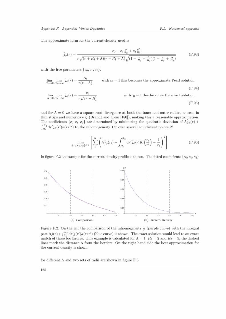
Appendix F. Appendix: Vortex Dynamics F.4. Numerical approach

The approximate form for the current-density used is

jφ(r) =c0 + c1

rR2

+ c2r2

R22

r√

(r +R1 + Λ)(r −R1 + Λ)√

(1− rR2

+ ΛR2

)(1 + rR2

+ ΛR2

)(F.93)

with the free parameters c0, c1, c2.

limR1→0

limR2→∞

jφ(r) =c0

r(r + Λ)with c0 = 1 this becomes the approximate Pearl solution

(F.94)

limΛ→0

limR2→∞

jφ(r) =c0

r√r2 −R2

1

with c0 = 1 this becomes the exact solution

(F.95)

and for Λ = 0 we have a square-root divergence at both the inner and outer radius, as seen inthin strips and numerics e.g. (Brandt and Clem [180]), making this a reasonable approximation.The coefficients c0, c1, c2 are determined by minimizing the quadratic deviation of Λjφ(r) +∫ R2

R1dr′jφ(r′)k(r/r′) to the inhomogeneity 1/r over several equidistant points N

minc0,c1,c2∈R

N∑i

(Λjφ(ri) +

∫ R2

R1

dr′jφ(r′)k(rir′

)− 1

ri

)2 (F.96)

In figure F.2 an example for the current density profile is shown. The fitted coefficients c0, c1, c2

2.5 3.0 3.5 4.0 4.5 5.0r

0.25

0.30

0.35

0.40

0.45

0.50

(a) Comparison

2.5 3.0 3.5 4.0 4.5 5.0r

0.10

0.15

0.20

0.25

0.30

jHrL

(b) Current Density

Figure F.2: On the left the comparison of the inhomogeneity 1r (purple curve) with the integral

part Λj(r)+∫ R2

R1dr′j(r′)k(r/r′) (blue curve) is shown. The exact solution would lead to an exact

match of these too figures. This example is calculated for Λ = 1, R1 = 2 and R2 = 5, the dashedlines mark the distance Λ from the borders. On the right hand side the best approximation forthe current density is shown.

for different Λ and two sets of radii are shown in figure F.3

168

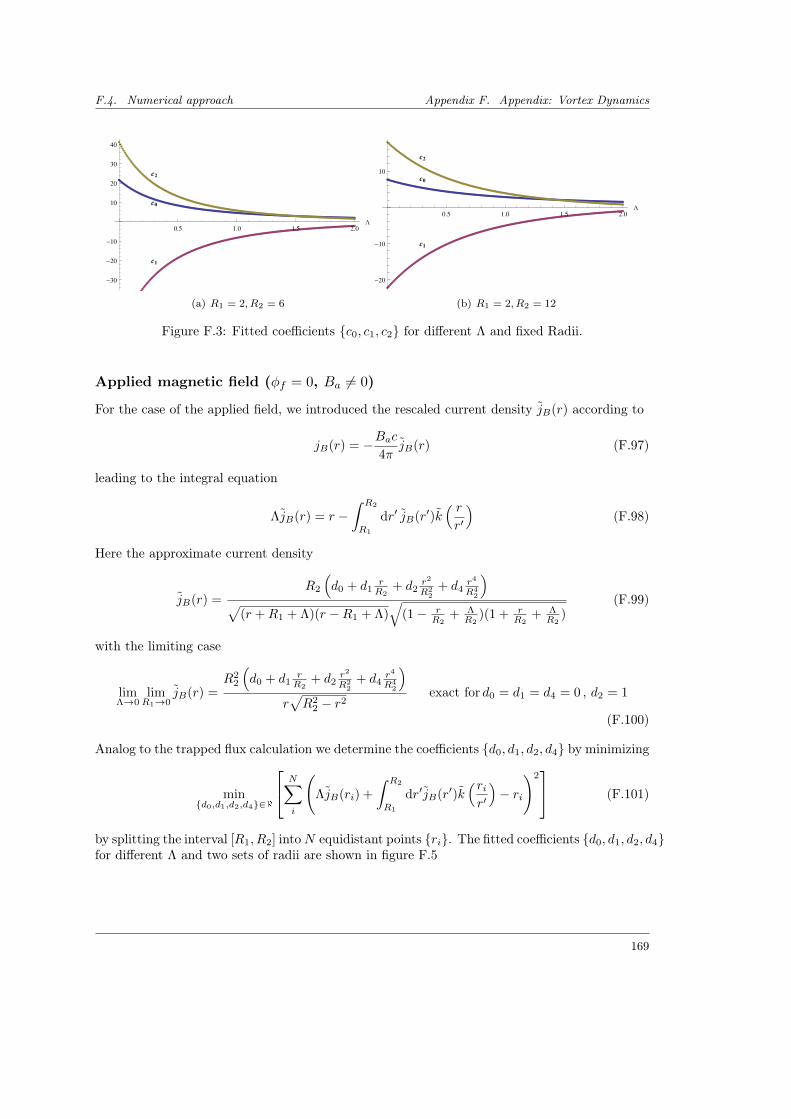
F.4. Numerical approach Appendix F. Appendix: Vortex Dynamics

0.5 1.0 1.5 2.0

L

-30

-20

-10

10

20

30

40

c0

c1

c2

(a) R1 = 2, R2 = 6

0.5 1.0 1.5 2.0

L

-20

-10

10

c0

c1

c2

(b) R1 = 2, R2 = 12

Figure F.3: Fitted coefficients c0, c1, c2 for different Λ and fixed Radii.

Applied magnetic field (φf = 0, Ba 6= 0)

For the case of the applied field, we introduced the rescaled current density jB(r) according to

jB(r) = −Bac4π

jB(r) (F.97)

leading to the integral equation

ΛjB(r) = r −∫ R2

R1

dr′ jB(r′)k( rr′

)(F.98)

Here the approximate current density

jB(r) =R2

(d0 + d1

rR2

+ d2r2

R22

+ d4r4

R42

)√

(r +R1 + Λ)(r −R1 + Λ)√

(1− rR2

+ ΛR2

)(1 + rR2

+ ΛR2

)(F.99)

with the limiting case

limΛ→0

limR1→0

jB(r) =R2

2

(d0 + d1

rR2

+ d2r2

R22

+ d4r4

R42

)r√R2

2 − r2exact for d0 = d1 = d4 = 0 , d2 = 1

(F.100)

Analog to the trapped flux calculation we determine the coefficients d0, d1, d2, d4 by minimizing

mind0,d1,d2,d4∈R

N∑i

(ΛjB(ri) +

∫ R2

R1

dr′jB(r′)k(rir′

)− ri

)2 (F.101)

by splitting the interval [R1, R2] intoN equidistant points ri. The fitted coefficients d0, d1, d2, d4for different Λ and two sets of radii are shown in figure F.5

169

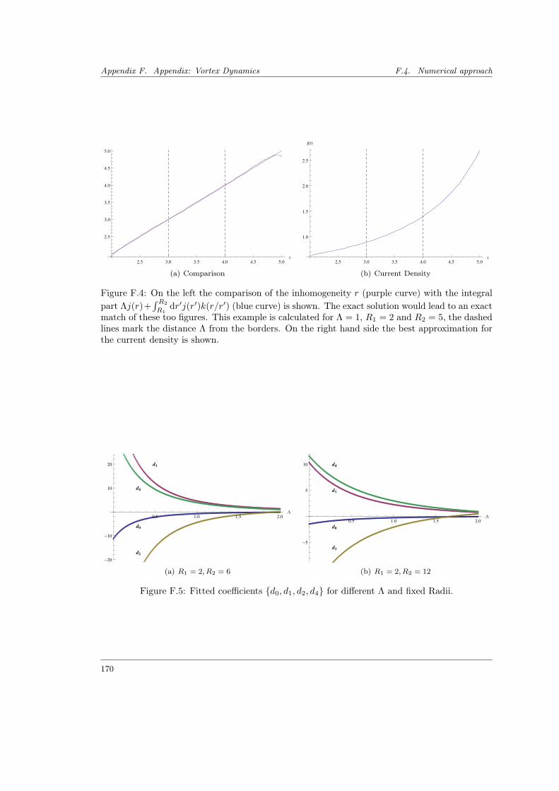
Appendix F. Appendix: Vortex Dynamics F.4. Numerical approach

2.5 3.0 3.5 4.0 4.5 5.0r

2.5

3.0

3.5

4.0

4.5

5.0

(a) Comparison

2.5 3.0 3.5 4.0 4.5 5.0r

1.0

1.5

2.0

2.5

jHrL

(b) Current Density

Figure F.4: On the left the comparison of the inhomogeneity r (purple curve) with the integralpart Λj(r)+

∫ R2

R1dr′j(r′)k(r/r′) (blue curve) is shown. The exact solution would lead to an exact

match of these too figures. This example is calculated for Λ = 1, R1 = 2 and R2 = 5, the dashedlines mark the distance Λ from the borders. On the right hand side the best approximation forthe current density is shown.

0.5 1.0 1.5 2.0

L

-20

-10

10

20

d0

d1

d4

d2

(a) R1 = 2, R2 = 6

0.5 1.0 1.5 2.0

L

-5

5

10

d0

d1

d4

d2

(b) R1 = 2, R2 = 12

Figure F.5: Fitted coefficients d0, d1, d2, d4 for different Λ and fixed Radii.

170

Bibliography

[1] D. P. Landau and E. M. Lifshitz. Statistical Physics. 1970.

[2] J. M. Yeomans. Statistical Mechanics of Phase Transitions. 1992.

[3] J. Cardy. Scaling and Renormalization in Statistical Physics. Cambridge Lecture Notes inPhysics 5. Cambridge University Press, 1996.

[4] S.-K. Ma. Modern Theory of Critical Phenomena. Frontiers in Physics. W. A. Bejamin,Inc., 1976.

[5] P. Chaikin and T. Lubensky. Principles of condensed matter physics. Cambridge, 1995.

[6] L. D. Landau and E. M. Lifshitz. Quantum Mechanics. Course of Theoretical Physics.Butterworth-Heinemann, 3rd edition, 1977.

[7] D. C. Mattis. The Theroy of of Magnetism. Springer Series in Solid-State Sciences. SpringerBerlin Heidelberg, 1981.

[8] A. Auerbach. Interacting Electrons and Quantum Magnetism. Graduate Texts in Contem-porary Physics. Springer Verlag, 1994.

[9] E. Ising. Beitrag zur Theorie des Ferromagnetismus. Zeitschrift für Physik, 31(1), 253–258,1925. ISSN 0044-3328.

[10] A. Altland and B. Simons. Condensed Matter Field Theory. Cambridge University Press,second edition, 2010.

[11] R. Peierls. On Ising’s model of ferromagnetism. Mathematical Proceedings of the CambridgePhilosophical Society, 32, 477–481, 10 1936. ISSN 1469-8064.

[12] L. Onsager. Crystal Statistics. I. A Two-Dimensional Model with an Order-Disorder Tran-sition. Phys. Rev., 65, 117–149, Feb 1944.

[13] N. Mermin and H. Wagner. Absence of Ferromagnetism or Antiferromagnetism in One-or Two-Dimensional Isotropic Heisenberg Models. Phys. Rev. Lett., 17, 1133–1136, Nov1966.

[14] V. L. Berezinskii. Violation of long range order in one-dimensional and two-dimensionalsystems with a continous symmetry group. I. Classical systems. JETP, 32, 493–500, 1971.

[15] J. M. Kosterlitz and D. J. Thouless. Ordering, metastability and phase transitions intwo-dimensional systems. Journal of Physics C: Solid State Physics, 6(7), 1181, 1973.

[16] J. Villain. La structure des substances magnetiques. Journal of Physics and Chemistry ofSolids, 11(3-4), 303–309, 1959. ISSN 0022-3697.

[17] A. Yoshimori. A New Type of Antiferromagnetic Structure in the Rutile Type Crystal.Journal of the Physical Society of Japan, 14(6), 807–821, 1959.

171

Bibliography Bibliography

[18] F. Li, T. Nattermann, and V. L. Pokrovsky. Vortex Domain Walls in Helical Magnets.Phys. Rev. Lett., 108, 107203, Mar 2012.

[19] M. Mostovoy. Ferroelectricity in Spiral Magnets. Phys. Rev. Lett., 96, 067601, Feb 2006.

[20] X. G. Wen, F. Wilczek, and A. Zee. Chiral spin states and superconductivity. Phys. Rev.B, 39, 11413–11423, Jun 1989.

[21] D. I. Khomskii. Spin chirality and nontrivial charge dynamics in frustrated Mott insulators:spontaneous currents and charge redistribution. Journal of Physics: Condensed Matter,22(16), 164209, 2010.

[22] A. Kolezhuk and T. Vekua. Field-induced chiral phase in isotropic frustrated spin chains.Phys. Rev. B, 72, 094424, Sep 2005.

[23] J.-C. Domenge, P. Sindzingre, C. Lhuillier, and L. Pierre. Twelve sublattice ordered phasein the J1-J2 model on the kagomé lattice. Phys. Rev. B, 72, 024433, Jul 2005.

[24] E. A. Turov. The Magnetism of the Rare-Earth Metals. In S. Krupcka and J. Sternberk,editors, Elements of Theoretical Magnetism. ILIFFE Books LTD, 1968.

[25] J. Jensen and A. R. Mackintosh. Rare Earth Magnetism Structures and Excitations.CLARENDON PRESS, 1991.

[26] P. G. DeGennes. Interactions indirectes entre couches 4f dans les métaux de terres rares.J. Phys. Radium, 23(8-9), 510–521, 1962.

[27] Y. Ishikawa, K. Tajima, D. Bloch, and M. Roth. Helical spin structure in manganesesilicide MnSi. Solid State Communications, 19(6), 525–528, jul 1976. ISSN 0038-1098.

[28] M. Uchida, Y. Onose, Y. Matsui, and Y. Tokura. Real-Space Observation of Helical SpinOrder. Science, 311(5759), 359–361, 2006.

[29] S. S. P. Parkin, M. Hayashi, and L. Thomas. Magnetic Domain-Wall Racetrack Memory.Science, 320(5873), 190–194, 2008.

[30] D. Khomskii. Classifying multiferroics: Mechanisms and effects. Physics, 2, 20, Mar 2009.

[31] S.-W. Cheong and M. Mostovoy. Multiferroics: a magnetic twist for ferroelectricity. NatMater, 6(1), 13–20, Jan 2007. ISSN 1476-1122. 10.1038/nmat1804.

[32] T.-H. Arima. Spin-Driven Ferroelectricity and Magneto-Electric Effects in Frustrated Mag-netic Systems. Journal of the Physical Society of Japan, 80(5), 052001, 2011.

[33] H. Katsura, N. Nagaosa, and A. V. Balatsky. Spin Current and Magnetoelectric Effect inNoncollinear Magnets. Phys. Rev. Lett., 95, 057205, Jul 2005.

[34] T. Kimura and Y. Tokura. Magnetoelectric phase control in a magnetic system showingcycloidal/conical spin order. Journal of Physics: Condensed Matter, 20(43), 434204, 2008.

[35] L. C. Chapon, G. R. Blake, M. J. Gutmann, S. Park, N. Hur, P. G. Radaelli, and S.-W. Cheong. Structural Anomalies and Multiferroic Behavior in Magnetically FrustratedTbMn2O5. Phys. Rev. Lett., 93, 177402, Oct 2004.

172

Bibliography Bibliography

[36] A. A. Bush, V. N. Glazkov, M. Hagiwara, T. Kashiwagi, S. Kimura, K. Omura, L. A.Prozorova, L. E. Svistov, A. M. Vasiliev, and A. Zheludev. Magnetic phase diagram of thefrustrated S = 1

2 chain magnet LiCu2O2. Phys. Rev. B, 85, 054421, Feb 2012.

[37] O. Heyer, N. Hollmann, I. Klassen, S. Jodlauk, L. Bohatý, P. Becker, J. A. Mydosh,T. Lorenz, and D. Khomskii. A new multiferroic material: MnWO 4. Journal of Physics:Condensed Matter, 18(39), L471, 2006.

[38] V. Gnezdilov, P. Lemmens, A. A. Zvyagin, V. O. Cheranovskii, K. Lamonova, Y. G.Pashkevich, R. K. Kremer, and H. Berger. Magnetic crossover and complex excitationspectrum of the ferromagnetic/antiferromagnetic spin- 1

2 chain system α-TeVO4. Phys.Rev. B, 78, 184407, Nov 2008.

[39] F. Cinti, A. Rettori, M. G. Pini, M. Mariani, E. Micotti, A. Lascialfari, N. Papinutto,A. Amato, A. Caneschi, D. Gatteschi, and M. Affronte. Two-Step Magnetic Ordering inQuasi-One-Dimensional Helimagnets: Possible Experimental Validation of Villain’s Con-jecture about a Chiral Spin Liquid Phase. Phys. Rev. Lett., 100, 057203, Feb 2008.

[40] H. Schenck, V. L. Pokrovsky, and T. Nattermann. Vector Chiral Phases in the Frustrated2D XY Model and Quantum Spin Chains. Phys. Rev. Lett., 112, 157201, Apr 2014.

[41] D. Niermann, C. P. Grams, P. Becker, L. Bohatý, H. Schenck, and J. Hemberger. CriticalSlowing Down near the Multiferroic Phase Transition in MnWO4. Phys. Rev. Lett., 114,037204, Jan 2015.

[42] S. Sachdev. Quantum Phase Transitions. Cambridge University Press, 1999.

[43] A. K. Kolezhuk. Large-S Approach to Chiral Phases in Frustrated Spin Chains. Progressof Theoretical Physics Supplement, 145, 29–36, 2002.

[44] P. Bak and D. Mukamel. Physical realizations of n ≥ 4-component vector models. III.Phase transitions in Cr, Eu, MnS2, Ho, Dy, and Tb. Phys. Rev. B, 13, 5086–5094, Jun1976.

[45] H. Kawamura. Erratum: Renormalization-group analysis of chiral transitions. Phys. Rev.B, 42, 2610–2610, Aug 1990.

[46] A. Hubert. Theorie der Domänenwände in geordneten Medien, volume 26 of Lecture Notesin Physics. Springer-Verlag Berlin, 1974.

[47] A. A. Nersesyan, A. O. Gogolin, and F. H. L. Eßler. Incommensurate Spin Correlations inSpin-1/2 Frustrated Two-Leg Heisenberg Ladders. Phys. Rev. Lett., 81, 910–913, Jul 1998.

[48] H. J. Mikeska and A. K. Kolezhuk. One-dimensional magnetism. Lecture Notes in Physicsvol. 645. Springer Verlag, 2004.

[49] H. Kawamura. Renormalization-group analysis of chiral transitions. Phys. Rev. B, 38,4916–4928, Sep 1988.

[50] H. Kawamura. Universality of phase transitions of frustrated antiferromagnets. Journal ofPhysics: Condensed Matter, 10(22), 4707, 1998.

[51] H. Schulz. Statistische Physik. Verlag Harri Deutsch, 2005.

173

Bibliography Bibliography

[52] A. L. Fetter and J. D. Walecka. Quantum Theory of Many-Particle Systems. McGraw-HillBook Company, 1971.

[53] A. Patashinskii and V. L. Pokrovskii. Fluctuation Theory of Phase Transitions. PergamonPress, 1979.

[54] E. Pytte. Spurious First-Order Phase Transitions in the Self-Consistent Phonon Approxi-mation. Phys. Rev. Lett., 28, 895–897, Apr 1972.

[55] R. M. Hornreich, M. Luban, and S. Shtrikman. Critical Behavior at the Onset of k-SpaceInstability on the λ-Line. Phys. Rev. Lett., 35, 1678–1681, Dec 1975.

[56] A. O. Sorokin and A. V. Syromyatnikov. Chiral spin liquid in two-dimensional XY heli-magnets. Phys. Rev. B, 85, 174404, May 2012.

[57] A. Sorokin and A. Syromyatnikov. Erratum: Chiral spin liquid in two-dimensional XYhelimagnets [Phys. Rev. B 85, 174404 (2012)]. Phys. Rev. B, 86, 059904, Aug 2012.

[58] E. Weschke, H. Ott, E. Schierle, C. Schüßler-Langeheine, D. V. Vyalikh, G. Kaindl,V. Leiner, M. Ay, T. Schmitte, H. Zabel, and P. J. Jensen. Finite-Size Effect on MagneticOrdering Temperatures in Long-Period Antiferromagnets: Holmium Thin Films. Phys.Rev. Lett., 93, 157204, Oct 2004.

[59] M. Hase, H. Kuroe, K. Ozawa, O. Suzuki, H. Kitazawa, G. Kido, and T. Sekine. Mag-netic properties of Rb2Cu2Mo3O12 including a one-dimensional spin-1/2 Heisenberg systemwith ferromagnetic first-nearest-neighbor and antiferromagnetic second-nearest-neighborexchange interactions. Phys. Rev. B, 70, 104426, Sep 2004.

[60] G. Castilla, S. Chakravarty, and V. J. Emery. Quantum Magnetism of CuGeO3. Phys.Rev. Lett., 75, 1823–1826, Aug 1995.

[61] J. Riera and A. Dobry. Magnetic susceptibility in the spin-Peierls system CuGeO3. Phys.Rev. B, 51, 16098–16102, Jun 1995.

[62] K. Hikomitsu, N. Hiroshi, A. Yoshitami, A. Takayuki, and G. Tsuneaki. Susceptibilityand high-field magnetization of one-dimensional S=12 Heisenberg antiferromagnet withnext-nearest exchange interaction. Physica B: Condensed Matter, 284-288, Part 2(0),1631–1632, jul 2000. ISSN 0921-4526.

[63] N. Maeshima, M. Hagiwara, Y. Narumi, K. Kindo, T. C. Kobayashi, and K. Okunishi.Magnetic properties of a S = 1/2 zigzag spin chain compound (N 2 H 5 )CuCl 3. Journalof Physics: Condensed Matter, 15(21), 3607, 2003.

[64] M. Hase, K. Ozawa, and N. Shinya. Magnetic properties of Cu6Ge6O18-xH2O (x=0–6): Acompound of S = 1/2 Heisenberg competing antiferromagnetic chains coupled by interchaininteraction. Phys. Rev. B, 68, 214421, Dec 2003.

[65] M. Hase, K. Ozawa, and N. Shinya. Magnetic properties of a three-dimensional antifer-romagnet formed by three bonds, Cu6Ge6O18-xH2O (x=0-6). Journal of Magnetism andMagnetic Materials, 272-276, Part 2(0), 869–871, 2004. ISSN 0304-8853.

[66] T. Masuda, A. Zheludev, A. Bush, M. Markina, and A. Vasiliev. Competition betweenHelimagnetism and Commensurate Quantum Spin Correlations in LiCu2O2. Phys. Rev.Lett., 92, 177201, Apr 2004.

174

Bibliography Bibliography

[67] G. Kamieniarz, M. Bielinski, G. Szukowski, R. Szymczak, S. Dyeyev, and J.-P. Renard.Finite temperature quantum transfer-matrix simulations of the frustrated spin-1/2 chains.Computer Physics Communications, 147(1-2), 716–719, 2002. ISSN 0010-4655.

[68] Y. Mizuno, T. Tohyama, S. Maekawa, T. Osafune, N. Motoyama, H. Eisaki, and S. Uchida.Electronic states and magnetic properties of edge-sharing Cu-O chains. Phys. Rev. B, 57,5326–5335, Mar 1998.

[69] M. Matsuda and K. Katsumata. Magnetic properties of a quasi-one-dimensional magnetwith competing interactions: SrCuO2. Journal of Magnetism and Magnetic Materials,140-144, Part 3(0), 1671–1672, Feb 1995. ISSN 0304-8853.

[70] M. Matsuda, K. Katsumata, K. M. Kojima, M. Larkin, G. M. Luke, J. Merrin, B. Nachumi,Y. J. Uemura, H. Eisaki, N. Motoyama, S. Uchida, and G. Shirane. Magnetic phasetransition in the S= zigzag-chain compound SrCuO2. Phys. Rev. B, 55, R11953–R11956,May 1997.

[71] T. Masuda, A. Zheludev, B. Roessli, A. Bush, M. Markina, and A. Vasiliev. Spin wavesand magnetic interactions in LiCu2O2. Phys. Rev. B, 72, 014405, Jul 2005.

[72] T. Masuda, A. Zheludev, A. Bush, M. Markina, and A. Vasiliev. Masuda et al. Reply:.Phys. Rev. Lett., 94, 039706, Jan 2005.

[73] H. Kikuchi, M. Chiba, and T. Kubo. Possible gapless chiral phase in a frustrated S = 11D anti-ferromagnet, CaV2O4. Canadian Journal of Physics, 79(11-12), 1551–1555, 2001.

[74] A. Lascialfari, R. Ullu, M. Affronte, F. Cinti, A. Caneschi, D. Gatteschi, D. Rovai, M. G.Pini, and A. Rettori. Specific heat and µ+SR measurements in Gd(hfac)3NITiPr molecularmagnetic chains: Indications for a chiral phase without long-range helical order. Phys. Rev.B, 67, 224408, Jun 2003.

[75] M. Affronte, A. Caneschi, C. Cucci, D. Gatteschi, J. C. Lasjaunias, C. Paulsen, M. G.Pini, A. Rettori, and R. Sessoli. Low-temperature thermodynamic properties of molecularmagnetic chains. Phys. Rev. B, 59, 6282–6293, Mar 1999.

[76] T. Nattermann. Private Communication, 2013.

[77] S. Kim. Vortex interaction in Josephson-junction ladders. Physics Letters A, 229(3),190–194, 1997. ISSN 0375-9601.

[78] F. Kusmartsev, D. Faruque, and D. Khomskii. Quasiclassical method for Josephson net-work in magnetic field. Physics Letters A, 249(5-6), 541–554, 1998. ISSN 0375-9601.

[79] A. A. Golubov, M. Y. Kupriyanov, and E. Il’ichev. The current-phase relation in Josephsonjunctions. Rev. Mod. Phys., 76, 411–469, Apr 2004.

[80] A. K. Feofanov, V. A. Oboznov, V. V. Bol’ginov, J. Lisenfeld, S. Poletto, V. V. Ryazanov,A. N. Rossolenko, M. Khabipov, D. Balashov, A. B. Zorin, P. N. Dmitriev, V. P. Koshelets,and A. V. Ustivnov. Implementation of superconductor/ferromagnet/ superconductor π-shifters in superconducting digital and quantum circuits. Nature, 6, 593–597, Jun 2010.

[81] O. Bourgeois, P. Gandit, A. Sulpice, J. Chaussy, J. Lesueur, and X. Grison. Transport insuperconductor/ferromagnet/superconductor junctions dominated by interface resistance.Phys. Rev. B, 63, 064517, Jan 2001.

175

Bibliography Bibliography

[82] E. Goldobin, D. Koelle, R. Kleiner, and R. G. Mints. Josephson Junction with a Magnetic-Field Tunable Ground State. Phys. Rev. Lett., 107, 227001, Nov 2011.

[83] P. Martinoli and C. Leemann. Two Dimensional Josephson Junction Arrays. Journal ofLow Temperature Physics, 118(5-6), 699–731, 2000. ISSN 0022-2291.

[84] S. Herbert, L. Gómez, D. Mast, R. Newrock, C. Wilks, and C. Falco. Fabrication of 3Dproximity coupled Josephson junction arrays. Superlattices and Microstructures, 18(1),53–, 1995. ISSN 0749-6036.

[85] J. Villain. Chiral order in helimagnets. Annals of the Israel Physical Society, 2, 565, 1978.

[86] T. Garel and S. Doniach. On the critical behaviour of two-dimensional XY helimagnets.Journal of Physics C: Solid State Physics, 13(31), L887, 1980.

[87] Y. Okwamoto. Phase Transitions of Two-Dimensional Helical XY Models. Journal of thePhysical Society of Japan, 53(8), 2613–2621, 1984.

[88] P. Lecheminant, T. Jolicoeur, and P. Azaria. Phase transitions in the one-dimensionalspin-SJ1−J2XY model. Phys. Rev. B, 63, 174426, Apr 2001.

[89] T. Hikihara, M. Kaburagi, and H. Kawamura. Ground-state phase diagrams of frustratedspin- S XXZ chains: Chiral ordered phases. Phys. Rev. B, 63, 174430, Apr 2001.

[90] O. Dimitrova. Chiral spin liquid in a two-dimensional two-component helical magnet. Phys.Rev. B, 90, 014409, Jul 2014.

[91] H. Kleinert and V. Schulte-Frohlinde. Critical Properties of φ4-Theories. World Scientific,2001.

[92] T.-H. Arima. Ferroelectricity Induced by Proper-Screw Type Magnetic Order. Journal ofthe Physical Society of Japan, 76(7), 073702, 2007.

[93] I. Dzyaloshinskii. Theory of Helicoidal Structures in Antiferromagnets. I. Nonmetals .JETP, 19(4), 960, 1964.

[94] T. Moriya. New Mechanism of Anisotropic Superexchange Interaction. Phys. Rev. Lett.,4, 228–230, Mar 1960.

[95] E. Soergel. Piezoresponse force microscopy (PFM). Journal of Physics D: Applied Physics,44(46), 464003, 2011.

[96] F. Chernous’ko. A local variation method for the numerical solution of variational problems.USSR Computational Mathematics and Mathematical Physics, 5(4), 234–242, 1965. ISSN0041-5553.

[97] A. Erdélyi, W. Magnus, F. Oberhettinger, and F. G. Tricomi. Higher TranscendentalFunctions, volume Vol I. McGraw-Hill Book Company, 1953.

[98] G. Lautenschläger, H. Weitzel, T. Vogt, R. Hock, A. Böhm, M. Bonnet, and H. Fuess.Magnetic phase transitions of MnWO4 studied by the use of neutron diffraction. Phys.Rev. B, 48, 6087–6098, Sep 1993.

[99] K. Taniguchi, N. Abe, T. Takenobu, Y. Iwasa, and T. Arima. Ferroelectric PolarizationFlop in a Frustrated Magnet MnWO4 Induced by a Magnetic Field. Phys. Rev. Lett., 97,097203, Aug 2006.

176

Bibliography Bibliography

[100] P. Tolédano, B. Mettout, W. Schranz, and G. Krexner. Directional magnetoelectric effectsin MnWO4 : magnetic sources of the electric polarization. Journal of Physics: CondensedMatter, 22(6), 065901, 2010.

[101] M. Hamermesh. Group Theory And Its Application To Physical Problems. Addison-WesleySeries In Physics. Addison-Wesley, 1962.

[102] O. Kovalev. Representations of the Crystallographic Space Groups. Gordon and BreachSicence Publishers, 2nd edition, 1993.

[103] K. Olbrychski. Abstract Definition and Representations of a Space Group. physica statussolidi (b), 3(10), 1868–1875, 1963. ISSN 1521-3951.

[104] E. F. Bertaut. Representation analysis of magnetic structures. Acta CrystallographicaSection A, 24(1), 217–231, 1968. ISSN 1600-5724.

[105] E. F. Bertraut. MAGNETIC STRUCTURE ANALYSIS AND GROUP THEORY. J.Phys. Colloques, 32, C1–462–C1–470, 1971.

[106] S. Matityahu, A. Aharony, and O. Entin-Wohlman. Landau theory for the phase diagramof multiferroic Mn1−x(Fe,Zn,Mg)xWO4. Phys. Rev. B, 85, 174408, May 2012.

[107] K. B. Varnashev. The stability of a cubic fixed point in three dimensions from the renor-malization group. Journal of Physics A: Mathematical and General, 33(16), 3121, 2000.

[108] A. Aharony. Critical Behavior of Magnets with Dipolar Interactions. III. Antiferromagnets.Phys. Rev. B, 8, 3349–3357, Oct 1973.

[109] A. Aharony. Dependence of Universal Critical Behaviour on Symmetry and Range of In-teraction. Phase Transitions and Critical Phenomena Vol. 6. Academic Press Inc. London,1976.

[110] E. Brézin, J. C. L. Guillou, and J. Zinn-Justin. Discussion of critical phenomena for generaln-vector models. Phys. Rev. B, 10, 892–900, Aug 1974.

[111] A. B. Harris, A. Aharony, and O. Entin-Wohlman. Order parameters and phase diagramsof multiferroics. Journal of Physics: Condensed Matter, 20(43), 434202, 2008.

[112] P. C. Hohenberg and B. I. Halperin. Theory of dynamic critical phenomena. Rev. Mod.Phys., 49, 435–479, Jul 1977.

[113] R. Folk and G. Moser. Critical dynamics: a field-theoretical approach. Journal of PhysicsA: Mathematical and General, 39(24), R207, 2006.

[114] V. Prudnikov, A. Ivanov, and A. Fedorenko. Critical dynamics of spin systems in the four-loop approximation. Journal of Experimental and Theoretical Physics Letters, 66(12),835–840, 1997. ISSN 0021-3640.

[115] S. Wansleben and D. P. Landau. Monte Carlo investigation of critical dynamics in thethree-dimensional Ising model. Phys. Rev. B, 43, 6006–6014, Mar 1991.

[116] H.-O. Heuer. Critical dynamics of the three-dimensional Ising model: A Monte Carlostudy. Journal of Statistical Physics, 72(3-4), 789–827, 1993. ISSN 0022-4715.

177

Bibliography Bibliography

[117] K. Lauritsen and N. Ito. Spectral method determination of dynamic exponents for Isingmodels. Physica A: Statistical Mechanics and its Applications, 202(1-2), 224–236, 1994.ISSN 0378-4371.

[118] R. Guida and J. Zinn-Justin. Critical exponents of the N -vector model. Journal of PhysicsA: Mathematical and General, 31(40), 8103, 1998.

[119] H. K. Onnes. Further experiments with liquid helium. C. On the change of electric resis-tance of pure metals at very low temperatures, etc. IV. The resistance of pure mercury athelium temperatures. Leiden Comm., (120b), 1911.

[120] H. K. Onnes. Further experiments with liquid helium. D. On the change of electric resis-tance of pure metals at very low temperatures, etc. V. The disappearance of the resistanceof mercury. Leiden Comm., (112b), 1911.

[121] H. K. Onnes. Further experiments with liquid helium. G. On the electrical resistance ofpure metals, etc. VI. On the sudden change in the rate at which the resistance of mercurydisappears. Leiden Comm., (124c), 1911.

[122] W. Meissner and R. Ochsenfeld. Ein neuer Effekt bei Eintritt der Supraleitflüssigkeit.Naturwissenschaften, 21(44), 787–788, 1933. ISSN 0028-1042.

[123] M. Tinkham. Introduction to Superconductivity. McGraw-Hill, 1996.

[124] A. A. Abrikosov. On the Magnetic Properties of Superconductors of the Second Group.Soviet Phys JETP, 5, 1174, 1957.

[125] J. Pearl. Current distribution in superconduction films carrying quantized fluxoids. AppliedPhysics Letters, 5(4), 65–66, 1964.

[126] J. Pearl. Distinctive properties of quantized vortices in superconducting films. Jan 1964.

[127] U. Essmann and H. Träuble. The direct observation of individual flux lines in type IIsuperconductors. Physics Letters A, 24(10), 526–527, may 1967. ISSN 0375-9601.

[128] A. Finkler, Y. Segev, Y. Myasoedov, M. L. Rappaport, L. Ne’eman, D. Vasyukov, E. Zeldov,M. E. Huber, J. Martin, and A. Yacoby. Self-Aligned Nanoscale SQUID on a Tip. NanoLetters, 10(3), 1046–1049, 2010. PMID: 20131810.

[129] T. Giamarchi and P. L. Doussal. Moving Glass Phase of Driven Lattices. Phys. Rev. Lett.,76, 3408–3411, Apr 1996.

[130] T. Giamarchi and P. L. Doussal. Bragg- and Moving-glasses: a theory of disordered vortexlattices. Physica C: Superconductivity, 282-287, Part 1(0), 363–366, 1997. ISSN 0921-4534.

[131] F. Pardo, F. de la Cruz, P. L. Gammel, E. Bucher, and D. Bishop. Observation of smecticand moving-Bragg-glass phases in flowing vortex lattices. Nature, 396, 348–350, Nov 1998.

[132] E. Zeldov and L. Embon. Private Communication. 2013.

[133] J. Bardeen, L. Cooper, and J. Schrieffer. Theory of Superconductivity. Phys. Rev., 108,1175–1204, Dec 1957.

[134] F. London and H. London. The Electromagnetic Equations of the Supraconductor. RoyalSociety of London Proceedings Series A, 149, 71–88, March 1935.

178

Bibliography Bibliography

[135] V. L. Ginzburg and L. D. Landau. To the Theory of Superconductivity. Eksp. Teor.Fiz., 20, 1064, 1950. [The English translation of this paper can be found in L.D. Landau,Collected Papers, Pergamon Press, Oxford, 1965].

[136] L. Gor’kov. Microscopic derivation of the Ginzubrg-Landau equations in the theory ofsuperconductivity. JETP, 36(9), 1364, 1959.

[137] A. L. Fetter and P. C. Hohenberg. The Mixed State of Thin Superconducting Films inPerpendicular Fields. Phys. Rev., 159, 330–343, Jul 1967.

[138] H. P. Myers. Introductory Solid State Physics. Taylor & Francis, 1997.

[139] J. Bass and K. H. Fischer. Group III Crystal and Solid State Physics, volume 15 of Landolt-Börnstein: Numerical Data and Functional Relationships in Science and Technology. 1982.

[140] G. D. Cody and R. E. Miller. Magnetic Transitions of Superconducting Thin Films andFoils. III. Pb, Sn, and In. Phys. Rev. B, 5, 1834–1843, Mar 1972.

[141] J. Bardeen and M. J. Stephen. Theory of the Motion of Vortices in Superconductors. Phys.Rev., 140, A1197–A1207, Nov 1965.

[142] V. Kopylov, A. Koshelev, I. Schegolev, and T. Togonidze. The role of surface effects inmagnetization of high-Tc superconductors. Physica C: Superconductivity, 170(3-4), 291–297, 1990. ISSN 0921-4534.

[143] L. Burlachkov. Magnetic relaxation over the Bean-Livingston surface barrier. Phys. Rev.B, 47, 8056–8064, Apr 1993.

[144] E. H. Brandt. Vortex-vortex interaction in thin superconducting films. Phys. Rev. B, 79,134526, Apr 2009.

[145] L. Burlachkov, V. B. Geshkenbein, A. E. Koshelev, A. I. Larkin, and V. M. Vinokur.Giant flux creep through surface barriers and the irreversibility line in high-temperaturesuperconductors. Phys. Rev. B, 50, 16770–16773, Dec 1994.

[146] P. W. Anderson and Y. B. Kim. Hard Superconductivity: Theory of the Motion ofAbrikosov Flux Lines. Rev. Mod. Phys., 36, 39–43, Jan 1964.

[147] M. R. Beasley, R. Labusch, and W. W. Webb. Flux Creep in Type-II Superconductors.Phys. Rev., 181, 682–700, May 1969.

[148] E. Zeldov, J. R. Clem, M. McElfresh, and M. Darwin. Magnetization and transport currentsin thin superconducting films. Phys. Rev. B, 49, 9802–9822, Apr 1994.

[149] E. H. Brandt and G. P. Mikitik. Meissner-London Currents in Superconductors withRectangular Cross Section. Phys. Rev. Lett., 85, 4164–4167, Nov 2000.

[150] I. L. Maksimov and A. A. Elistratov. Edge barrier and structure of the critical state insuperconducting thin films. JETP Letters, 61(3), 208, 1995.

[151] T. Schuster, H. Kuhn, and E. H. Brandt. Flux penetration into flat superconductors ofarbitrary shape: Patterns of magnetic and electric fields and current. Phys. Rev. B, 54,3514–3524, Aug 1996.

[152] A. A. B. Brojeny and J. R. Clem. Magnetic-field and current-density distributions inthin-film superconducting rings and disks. Phys. Rev. B, 68, 174514, Nov 2003.

179

Bibliography Bibliography

[153] E. H. Brandt and M. Indenbom. Type-II-superconductor strip with current in a perpen-dicular magnetic field. Phys. Rev. B, 48, 12893–12906, Nov 1993.

[154] L. Prigozhin. Solution of Thin Film Magnetization Problems in Type-II Superconductivity.Journal of Computational Physics, 144(1), 180–193, 1998. ISSN 0021-9991.

[155] E. H. Brandt. Supercurrents and vortices in SQUIDs and films of various shapes. PhysicaC: Superconductivity, 460-462, Part 1(0), 327–330, 2007. ISSN 0921-4534.

[156] E. H. Brandt. Thin superconductors and SQUIDs in perpendicular magnetic field. Phys.Rev. B, 72, 024529, Jul 2005.

[157] E. Bronson, M. P. Gelfand, and S. B. Field. Equilibrium configurations of Pearl vorticesin narrow strips. Phys. Rev. B, 73, 144501, Apr 2006.

[158] M. B. Ketchen, W. J. Gallagher, A. W. Kleinsasser, S. Murphy, and J. R. Clem. DCSquid Flux Focuser. SQUID ’85 - Superconducting Quantum Interference Devices andtheir Applications, pages 865–871. de Gruyter, 1985.

[159] L. Radzihovsky. Thermal depinning and transverse-field tilting transitions in a planarvortex array pinned by a columnar defect. Phys. Rev. B, 73, 104504, Mar 2006.

[160] A. Prudnikov, Y. Brychkov, and O. Marichev. Volume 2: Special Functions. 2, 1998.

[161] O. Narayan and D. Fisher. Nonlinear fluid flow in random media: Critical phenomena nearthreshold. Phys. Rev. B, 49, 9469–9502, Apr 1994.

[162] D. W. Braun, G. W. Crabtree, H. G. Kaper, A. E. Koshelev, G. K. Leaf, D. M. Levine,and V. M. Vinokur. Structure of a Moving Vortex Lattice. Phys. Rev. Lett., 76, 831–834,Jan 1996.

[163] L. Elliott, S. Theodore, and M. Daniel. Two soluble models of an antiferromagnetic chain.Annals of Physics, 16(3), 407–466, dec 1961. ISSN 0003-4916.

[164] F. D. M. Haldane. ’Luttinger liquid theory’ of one-dimensional quantum fluids. I. Propertiesof the Luttinger model and their extension to the general 1D interacting spinless Fermigas. Journal of Physics C: Solid State Physics, 14(19), 2585, 1981.

[165] A. Dutta, U. Divakaran, D. Sen, B. K. Chakrabarti, T. F. Rosenbaum, and G. Aeppli.Quantum phase transitions in transverse field spin models: From Statistical Physics toQuantum Information. ArXiv e-prints, December 2010.

[166] T. Holstein and H. Primakoff. Field Dependence of the Intrinsic Domain Magnetization ofa Ferromagnet. Phys. Rev., 58, 1098–1113, Dec 1940.

[167] P. W. Anderson. An Approximate Quantum Theory of the Antiferromagnetic GroundState. Phys. Rev., 86, 694–701, Jun 1952.

[168] R. Kubo. The Spin-Wave Theory of Antiferromagnetics. Phys. Rev., 87, 568–580, Aug1952.

[169] E. Fradkin. Field Theories of Condensed Matter Systems. Frontiers in Physics. Addison-Wesley Publishing Company, 1991.

[170] E. Manousakis. The spin- 12 Heisenberg antiferromagnet on a square lattice and its appli-

cation to the cuprous oxides. Rev. Mod. Phys., 63, 1–62, Jan 1991.

180

Bibliography Bibliography

[171] A. K. Kolezhuk. Quantum chiral phases in frustrated easy-plane spin chains. Phys. Rev.B, 62, R6057–R6060, Sep 2000.

[172] C. Kittel. Einführung in die Festkörperphysik. Oldenbourg, 8 edition, 1989.

[173] A. W. Manjunath, T. Sankarappa, R. Ramanna, J. S. Ashwajeet, T. Sujatha, and P. Sar-vanan. Low Temperature Electrical Resisitivity Studies in Lead Thin Films. Journal ofNano- and Electronic Physics, 5(3), 03026, 2013.

[174] A. Eiling and J. S. Schilling. Pressure and temperature dependence of electrical resistivityof Pb and Sn from 1-300K and 0-10 GPa-use as continuous resistive pressure monitoraccurate over wide temperature range; superconductivity under pressure in Pb, Sn and In.Journal of Physics F: Metal Physics, 11(3), 623, 1981.

[175] R. E. Glover. Currents and Fields in a Superconducting Film Carrying a Steady Current:Discussion. In G. M. Graham and A. C. H. Hallett, editors, Proceedings of the VIIthInternational Conference on Low Temperature Physics, page 416. Univeristy of TorontoPress: Toronto, 1961. see discussion of paper by Marcus.

[176] L. N. Cooper. Current Flow in Thin Superconducting Films. In G. M. Graham and A. C. H.Hallett, editors, Proceedings of the VIIth International Conference on Low TemperaturePhysics, page 416. Univeristy of Toronto Press: Toronto, 1961.

[177] P. M. Marcus. Currents and Fields in a Superconducting Film Carrying a Steady Current.In G. M. Graham and A. C. H. Hallett, editors, Proceedings of the VIIth InternationalConference on Low Temperature Physics, page 418. Univeristy of Toronto Press: Toronto,1961.

[178] E. H. Rhoderick and E. M. Wilson. Current Distribution in Thin Superconducting Films.Nature, 194(4834), 1167–1168, jun 1962. 10.1038/1941167b0.

[179] R. E. Glover and H. T. Coffey. Critical Currents in Thin Planar Films. Rev. Mod. Phys.,36, 299–302, Jan 1964.

[180] E. H. Brandt and J. R. Clem. Superconducting thin rings with finite penetration depth.Phys. Rev. B, 69, 184509, May 2004.

181

Ich versichere, dass ich die von mir vorgelegte Dissertation selbständig angefertigt, die be-nutzten Quellen und Hilfsmittel vollständig angegeben und die Stell der Arbeit - einschließlichTabellen, Karten und Abbildungen -, die anderen Werken im Wortlaut oder dem Sinn nach ent-nommen sind, in jedem Einzelfall als Entlehnung kenntlich gemacht habe; dass diese Dissertationnoch keiner anderen Fakultät oder Universität zur Prüfung vorgelegen hat; dass sie - abgesehenvon unten angegebenen Teilpublikationen - noch nicht veröffentlicht worden ist sowie, dass icheine solche Veröffentlichung vor Abschluss des Promotionsverfahrens nicht vornehmen werde. DieBestimmungen der Promotionsordnung sind mir bekannt. Die von mir vorgelegte Dissertationist von Prof. Dr. Thomas Nattermann betreut worden

Ort, Datum Hannes Schenck

Teilpublikationen:

• H. Schenck, V. L. Pokrovsky and T. NattermannVector chiral phases in frustrated 2D XY model and quantum spin chainsPhysical Review Letters 112 157201 (2014)

• D. Niermann, C. P. Grams, P. Becker, L. Bohatý, H. Schenck and J. HembergerCritical slowing down near the multiferroic phase transition in MnWO4Physical Review Letters 114 037204 (2015)