Vector autoregressions, VARChapter 2

Financial EconometricsMichael Hauser

WS17/18

1 / 45

Content

I Cross-correlationsI VAR model in standard/reduced formI Properties of VAR(1), VAR(p)I Structural VAR, identificationI Estimation, model specification, forecastingI Impulse responses

Everybody should recapitulate the properties of univariate AR(1) models !

2 / 45

Notation

Here we use the multiple equations notation. Vectors are of the form:yt = (y1t , . . . , ykt)

′ a cloumn vector of length k .yt contains the values of k variables at time t .k . . . the number of variables (i.g. number of equations)T . . . the number of observations

We do not distinguish in notation between data and random variables.

3 / 45

Motivation

4 / 45

Multivariate data

From an empirical/atheoretical point of view observed time series movements areoften related with each another. E.g.

I GDP growth and unemployment rate show an inverse pattern,I oil prices might be a leading indicator for other energy prices, which on the

other hand have an effect on oil.

5 / 45

Weak stationarity: multivariate

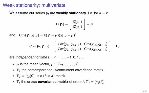
We assume our series yt are weakly stationary. I.e. for k = 2

E(yt) =

[E(y1t)

E(y2t)

]= µ

and Cov(yt ,yt−ℓ) = E(yt − µ)(yt−ℓ − µ)′

Cov(yt ,yt−ℓ) =

[Cov(y1t , y1,t−ℓ) Cov(y1t , y2,t−ℓ)

Cov(y2t , y1,t−ℓ) Cov(y2t , y2,t−ℓ)

]= Γℓ

are independent of time t . ℓ = . . . ,−1,0,1, . . . .

I µ is the mean vector, µ = (µ1, . . . , µk )′.

I Γ0 the contemporaneous/concurrent covariance matrixI Γ0 = [γij(0)] is a (k × k) matrix.I Γℓ the cross-covariance matrix of order ℓ, Γℓ = [γij(ℓ)]

6 / 45

Cross-correlations

7 / 45

Cross-correlation matrices, CCMs

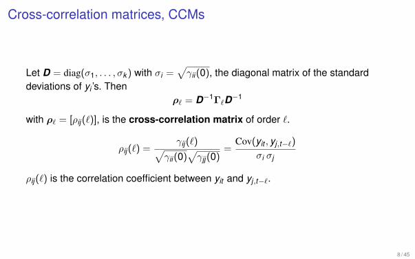
Let D = diag(σ1, . . . , σk ) with σi =√γii(0), the diagonal matrix of the standard

deviations of yi ’s. Thenρℓ = D−1ΓℓD−1

with ρℓ = [ρij(ℓ)], is the cross-correlation matrix of order ℓ.

ρij(ℓ) =γij(ℓ)√

γii(0)√γjj(0)

=Cov(yit , yj,t−ℓ)

σi σj

ρij(ℓ) is the correlation coefficient between yit and yj,t−ℓ.

8 / 45

Cross-correlation matrices: properties

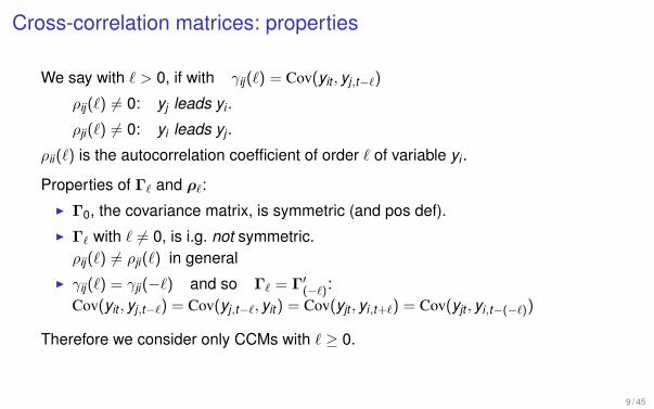
We say with ℓ > 0, if with γij(ℓ) = Cov(yit , yj,t−ℓ)

ρij(ℓ) = 0: yj leads yi .

ρji(ℓ) = 0: yi leads yj .

ρii(ℓ) is the autocorrelation coefficient of order ℓ of variable yi .

Properties of Γℓ and ρℓ:I Γ0, the covariance matrix, is symmetric (and pos def).I Γℓ with ℓ = 0, is i.g. not symmetric.ρij(ℓ) = ρji(ℓ) in general

I γij(ℓ) = γji(−ℓ) and so Γℓ = Γ′(−ℓ):

Cov(yit , yj,t−ℓ) = Cov(yj,t−ℓ, yit) = Cov(yjt , yi,t+ℓ) = Cov(yjt , yi,t−(−ℓ))

Therefore we consider only CCMs with ℓ ≥ 0.

9 / 45

Types of relationships

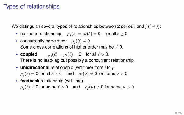
We distinguish several types of relationships between 2 series i and j (i = j):I no linear relationship: ρij(ℓ) = ρji(ℓ) = 0 for all ℓ ≥ 0I concurrently correlated: ρij(0) = 0

Some cross-correlations of higher order may be = 0.I coupled: ρij(ℓ) = ρji(ℓ) = 0 for all ℓ > 0.

There is no lead-lag but possibly a concurrent relationship.I unidirectional relationship (wrt time) from i to j :ρij(ℓ) = 0 for all ℓ > 0 and ρji(ν) = 0 for some ν > 0

I feedback relationship (wrt time):ρij(ℓ) = 0 for some ℓ > 0 and ρji(ν) = 0 for some ν > 0

10 / 45

Sample cross-correlations, properties

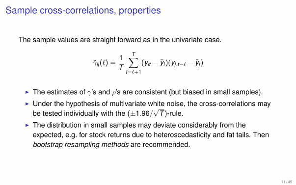
The sample values are straight forward as in the univariate case.

γij(ℓ) =1T

T∑t=ℓ+1

(yit − yi)(yj,t−ℓ − yj)

I The estimates of γ’s and ρ’s are consistent (but biased in small samples).I Under the hypothesis of multivariate white noise, the cross-correlations may

be tested individually with the (±1.96/√

T )-rule.I The distribution in small samples may deviate considerably from the

expected, e.g. for stock returns due to heteroscedasticity and fat tails. Thenbootstrap resampling methods are recommended.

11 / 45

Cross-correlations and autocorrelated yi ’s

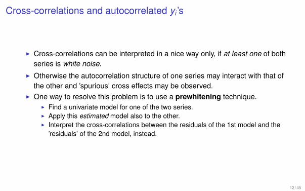
I Cross-correlations can be interpreted in a nice way only, if at least one of bothseries is white noise.

I Otherwise the autocorrelation structure of one series may interact with that ofthe other and ’spurious’ cross effects may be observed.

I One way to resolve this problem is to use a prewhitening technique.I Find a univariate model for one of the two series.I Apply this estimated model also to the other.I Interpret the cross-correlations between the residuals of the 1st model and the

’residuals’ of the 2nd model, instead.

12 / 45

Multivariate portmanteau test

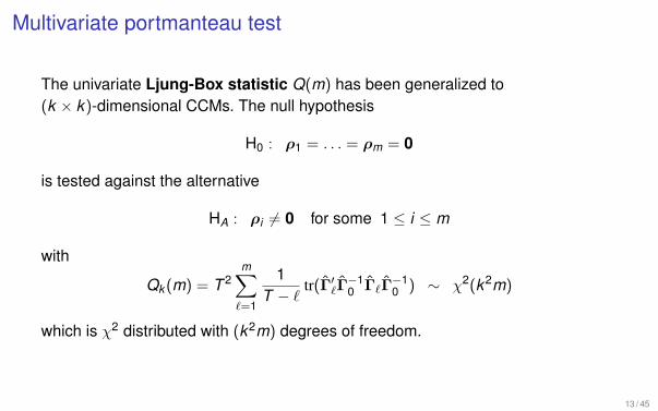
The univariate Ljung-Box statistic Q(m) has been generalized to(k × k)-dimensional CCMs. The null hypothesis

H0 : ρ1 = . . . = ρm = 0

is tested against the alternative

HA : ρi = 0 for some 1 ≤ i ≤ m

with

Qk (m) = T 2m∑ℓ=1

1T − ℓ

tr(Γ′ℓΓ

−10 ΓℓΓ

−10 ) ∼ χ2(k2m)

which is χ2 distributed with (k2m) degrees of freedom.

13 / 45

Multivariate portmanteau test

This test is suitable for the case where the interdependence of essentially(univariate) white noise returns is in question.

If only a single series is not white noise, i.e. ρii(ℓ) = 0 for some ℓ > 0, the test willreject as the univariate tests will do.

14 / 45

The VAR model

15 / 45

The VAR in standard form

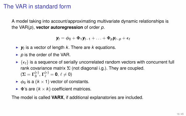
A model taking into account/approximating multivariate dynamic relationships isthe VAR(p), vector autoregression of order p.

yt = ϕ0 +Φ1yt−1 + . . .+Φpyt−p + ϵt

I yt is a vector of length k . There are k equations.I p is the order of the VAR.I ϵt is a sequence of serially uncorrelated random vectors with concurrent full

rank covariance matrix Σ (not diagonal i.g.). They are coupled.(Σ = Γ

(ϵ)0 , Γ(ϵ)

ℓ = 0, ℓ = 0)I ϕ0 is a (k × 1) vector of constants.I Φ’s are (k × k) coefficient matrices.

The model is called VARX, if additional explanatories are included.

16 / 45

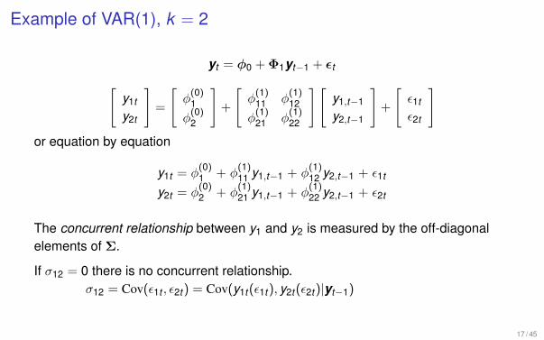
Example of VAR(1), k = 2

yt = ϕ0 +Φ1yt−1 + ϵt[y1t

y2t

]=

[ϕ(0)1

ϕ(0)2

]+

[ϕ(1)11 ϕ

(1)12

ϕ(1)21 ϕ

(1)22

][y1,t−1

y2,t−1

]+

[ϵ1t

ϵ2t

]or equation by equation

y1t = ϕ(0)1 + ϕ

(1)11 y1,t−1 + ϕ

(1)12 y2,t−1 + ϵ1t

y2t = ϕ(0)2 + ϕ

(1)21 y1,t−1 + ϕ

(1)22 y2,t−1 + ϵ2t

The concurrent relationship between y1 and y2 is measured by the off-diagonalelements of Σ.

If σ12 = 0 there is no concurrent relationship.σ12 = Cov(ϵ1t , ϵ2t) = Cov(y1t(ϵ1t), y2t(ϵ2t)|yt−1)

17 / 45

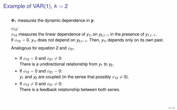
Example of VAR(1), k = 2

Φ1 measures the dynamic dependence in y .

ϕ12:ϕ12 measures the linear dependence of y1t on y2,t−1 in the presence of y1,t−1.If ϕ12 = 0, y1t does not depend on y2,t−1. Then, y1t depends only on its own past.

Analogous for equation 2 and ϕ21.

I If ϕ12 = 0 and ϕ21 = 0:There is a unidirectional relationship from y1 to y2.

I If ϕ12 = 0 and ϕ21 = 0:y1 and y2 are coupled (in the sense that possibly σ12 = 0).

I If ϕ12 = 0 and ϕ21 = 0:There is a feedback relationship between both series.

18 / 45

Properties of the VAR

19 / 45

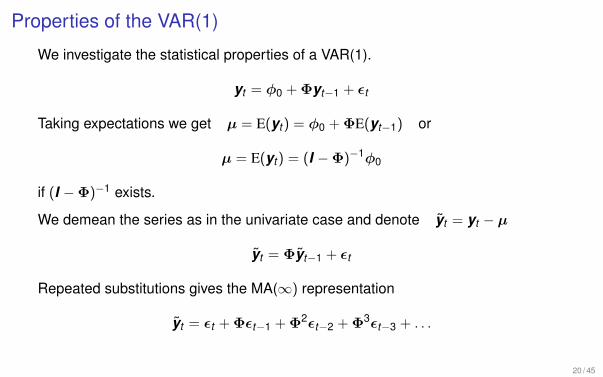
Properties of the VAR(1)

We investigate the statistical properties of a VAR(1).

yt = ϕ0 +Φyt−1 + ϵt

Taking expectations we get µ = E(yt) = ϕ0 +ΦE(yt−1) or

µ = E(yt) = (I −Φ)−1ϕ0

if (I −Φ)−1 exists.

We demean the series as in the univariate case and denote yt = yt − µ

yt = Φyt−1 + ϵt

Repeated substitutions gives the MA(∞) representation

yt = ϵt +Φϵt−1 +Φ2ϵt−2 +Φ3ϵt−3 + . . .

20 / 45

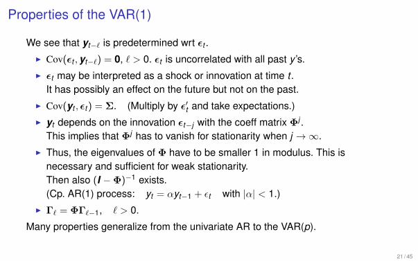
Properties of the VAR(1)

We see that yt−ℓ is predetermined wrt ϵt .I Cov(ϵt ,yt−ℓ) = 0, ℓ > 0. ϵt is uncorrelated with all past y ’s.I ϵt may be interpreted as a shock or innovation at time t .

It has possibly an effect on the future but not on the past.I Cov(yt , ϵt) = Σ. (Multiply by ϵ′t and take expectations.)I yt depends on the innovation ϵt−j with the coeff matrix Φj .

This implies that Φj has to vanish for stationarity when j → ∞.I Thus, the eigenvalues of Φ have to be smaller 1 in modulus. This is

necessary and sufficient for weak stationarity.Then also (I −Φ)−1 exists.(Cp. AR(1) process: yt = αyt−1 + ϵt with |α| < 1.)

I Γℓ = ΦΓℓ−1, ℓ > 0.

Many properties generalize from the univariate AR to the VAR(p).

21 / 45

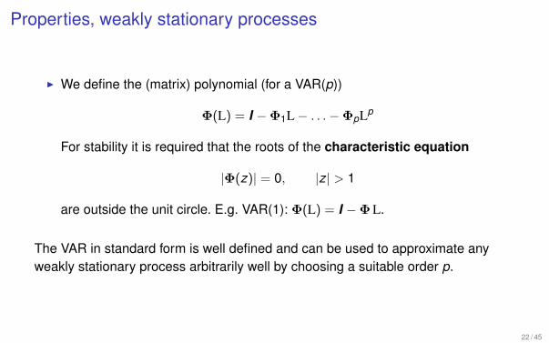
Properties, weakly stationary processes

I We define the (matrix) polynomial (for a VAR(p))

Φ(L) = I −Φ1L − . . .−ΦpLp

For stability it is required that the roots of the characteristic equation

|Φ(z)| = 0, |z| > 1

are outside the unit circle. E.g. VAR(1): Φ(L) = I −ΦL.

The VAR in standard form is well defined and can be used to approximate anyweakly stationary process arbitrarily well by choosing a suitable order p.

22 / 45

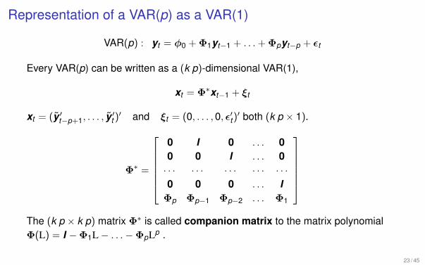
Representation of a VAR(p) as a VAR(1)

VAR(p) : yt = ϕ0 +Φ1yt−1 + . . .+Φpyt−p + ϵt

Every VAR(p) can be written as a (k p)-dimensional VAR(1),

xt = Φ∗xt−1 + ξt

xt = (y ′t−p+1, . . . , y

′t )

′ and ξt = (0, . . . , 0, ϵ′t)′ both (k p × 1).

Φ∗ =

0 I 0 . . . 00 0 I . . . 0· · · · · · · · · · · · · · ·0 0 0 . . . IΦp Φp−1 Φp−2 . . . Φ1

The (k p × k p) matrix Φ∗ is called companion matrix to the matrix polynomialΦ(L) = I −Φ1L − . . .−ΦpLp .

23 / 45

Representation of a VAR(p) as a VAR(1)

The last component of xt is the mean corrected yt , yt .

The last row of Φ∗ is essentially the VAR(p) recursion in reverse order.

24 / 45

Structural VAR and identification

25 / 45

Structural VAR

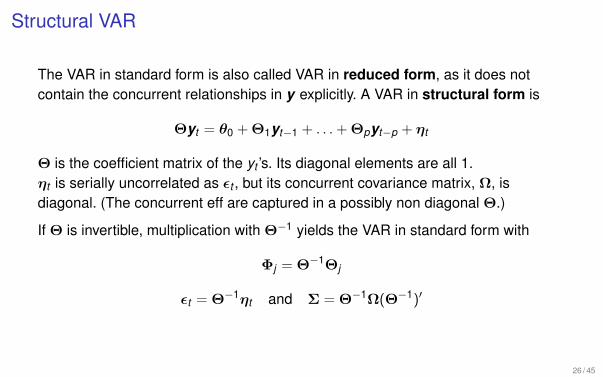
The VAR in standard form is also called VAR in reduced form, as it does notcontain the concurrent relationships in y explicitly. A VAR in structural form is

Θyt = θ0 +Θ1yt−1 + . . .+Θpyt−p + ηt

Θ is the coefficient matrix of the yt ’s. Its diagonal elements are all 1.ηt is serially uncorrelated as ϵt , but its concurrent covariance matrix, Ω, isdiagonal. (The concurrent eff are captured in a possibly non diagonal Θ.)

If Θ is invertible, multiplication with Θ−1 yields the VAR in standard form with

Φj = Θ−1Θj

ϵt = Θ−1ηt and Σ = Θ−1Ω(Θ−1)′

26 / 45

Identification

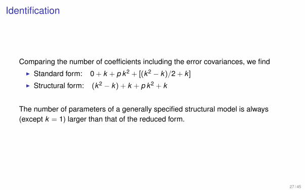
Comparing the number of coefficients including the error covariances, we findI Standard form: 0 + k + p k2 + [(k2 − k)/2 + k ]I Structural form: (k2 − k) + k + p k2 + k

The number of parameters of a generally specified structural model is always(except k = 1) larger than that of the reduced form.

27 / 45

Identification

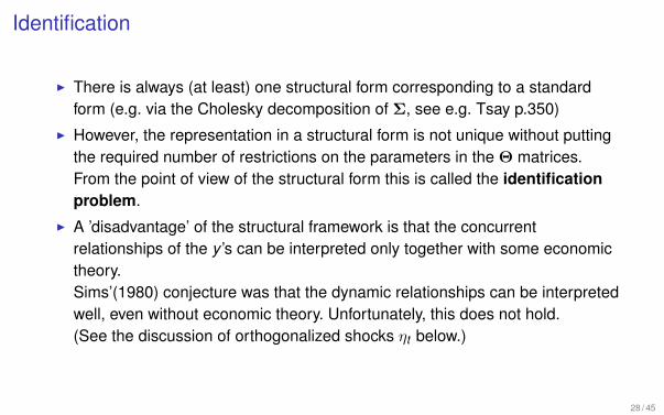
I There is always (at least) one structural form corresponding to a standardform (e.g. via the Cholesky decomposition of Σ, see e.g. Tsay p.350)

I However, the representation in a structural form is not unique without puttingthe required number of restrictions on the parameters in the Θ matrices.From the point of view of the structural form this is called the identificationproblem.

I A ’disadvantage’ of the structural framework is that the concurrentrelationships of the y ’s can be interpreted only together with some economictheory.Sims’(1980) conjecture was that the dynamic relationships can be interpretedwell, even without economic theory. Unfortunately, this does not hold.(See the discussion of orthogonalized shocks ηt below.)

28 / 45

Estimation of a VAR in standard form

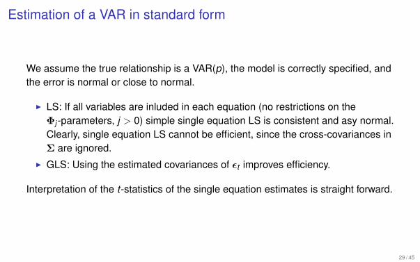
We assume the true relationship is a VAR(p), the model is correctly specified, andthe error is normal or close to normal.

I LS: If all variables are inluded in each equation (no restrictions on theΦj -parameters, j > 0) simple single equation LS is consistent and asy normal.Clearly, single equation LS cannot be efficient, since the cross-covariances inΣ are ignored.

I GLS: Using the estimated covariances of ϵt improves efficiency.

Interpretation of the t-statistics of the single equation estimates is straight forward.

29 / 45

Curse of dimensionality

A VAR(p) in standard form hasp k2

parameters not counting the constant terms and the error variance-covariances.

The number of the parameters isI linear in the order of the VAR, andI increases quadratically with the dimension k .

The number of observations (k T ) increases only linearly with k .

Remark: Emperically, it is difficult to interpret e.g. a significant Φ(9)7,23.

30 / 45

Model selection

Like in the univariate ARMA modeling, single coefficients in Φj , j > 0, are not setto zero a priori.The model selection procedure starts with a maximal plausible order pmax . Allmodels with p = 0,1, . . . , pmax are estimated. The models can be rankedaccording to an information criterion.The (conditional) ML estimate of the concurrent error covariance matrix of themodel with order p is

Σ(p) =1T

T∑t=p+1

ϵt(p) ϵ′t(p)

The model selection criteria are [log(|Σ(p)|) ≈ −(2/T ) ℓℓ(p)]

AIC(p) = log(|Σ(p)|) + 2 p k2/T

SBC(p) = log(|Σ(p)|) + log(T )p k2/T

31 / 45

Model validity

As in the univariate case the residuals of the chosen model should be(multivariate) white noise. Here the ρ

(ϵ)ℓ for ℓ > 0 should be zero.

The multivariate Ljung-Box test may be applied with number of freedoms as thenumber of cross-correlation coefficients under test reduced for the number ofestimated parameters:

k2(m − p)

32 / 45

Forecasting

33 / 45

Forecasting

Existing concurrent structural relationships between the endogenous variables aredemanding to interpret. However, due to the unique representation of thereduced/standard form the model is suitable for forecasting.

The 1-step ahead forecast (conditional on data up to T ) is

yT (1) = ϕ0 +Φ1yT + . . .+ΦpyT−p+1

The 1-step ahead forecast error, eT (1) = yT+1 − yT (1), is

eT (1) = ϵT+1

34 / 45

Forecasting

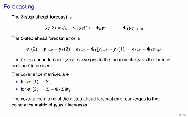
The 2-step ahead forecast is

yT (2) = ϕ0 +Φ1yT (1) +Φ2yT + . . .+ΦpyT−p+2

The 2-step ahead forecast error is

eT (2) = yT+2 − yT (2) = ϵT+2 +Φ1[yT+1 − yT (1)] = ϵT+2 +Φ1ϵT+1

The ℓ-step ahead forecast yT (ℓ) converges to the mean vector µ as the forecasthorizon ℓ increases.

The covariance matrices areI for eT (1) Σ,I for eT (2) Σ+Φ1ΣΦ′

1.

The covariance matrix of the ℓ-step ahead forecast error converges to thecovariance matrix of yt as ℓ increases.

35 / 45

Impulse responses

36 / 45

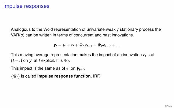
Impulse responses

Analogous to the Wold representation of univariate weakly stationary process theVAR(p) can be written in terms of concurrent and past innovations.

yt = µ+ ϵt +Ψ1ϵt−1 +Ψ2ϵt−2 + . . .

This moving average representation makes the impact of an innovation ϵt−i at(t − i) on yt at t explicit. It is Ψi .

This impact is the same as of ϵt on yt+i .

Ψi is called impulse response function, IRF.

37 / 45

Impulse responses

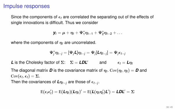
Since the components of ϵt are correlated the separating out of the effects ofsingle innovations is difficult. Thus we consider

yt = µ+ ηt +Ψ∗1ηt−1 +Ψ∗

2ηt−2 + . . .

where the components of ηt are uncorrelated.

Ψ∗j ηt−j = [ΨjL]ηt−j = Ψj [Lηt−j ] = Ψjϵt−j

L is the Cholesky factor of Σ: Σ = LDL′ and ϵt = Lηt

The diagonal matrix D is the covariance matrix of ηt . Cov(ηt ,ηt) = D andCov(ϵt , ϵt) = Σ.Then the covariances of Lηt−j are those of ϵt−j .

E(ϵtϵ′t) = E(Lηt)(Lηt)

′ = E(L(ηtη′t)L

′) = LDL′ = Σ

38 / 45

Impulse responses

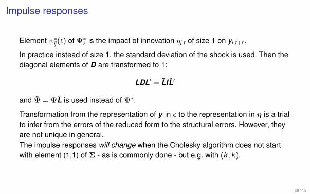
Element ψ∗ij (ℓ) of Ψ∗

ℓ is the impact of innovation ηj,t of size 1 on yi,t+ℓ.

In practice instead of size 1, the standard deviation of the shock is used. Then thediagonal elements of D are transformed to 1:

LDL′ = LIL′

and Ψ = ΨL is used instead of Ψ∗.

Transformation from the representation of y in ϵ to the representation in η is a trialto infer from the errors of the reduced form to the structural errors. However, theyare not unique in general.The impulse responses will change when the Cholesky algorithm does not startwith element (1,1) of Σ - as is commonly done - but e.g. with (k , k).

39 / 45

Exercise and References

40 / 45

Exercises

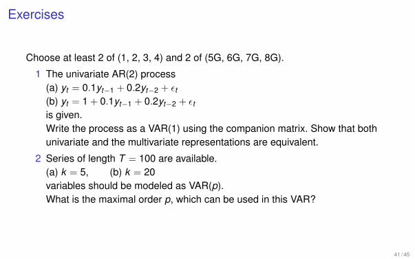
Choose at least 2 of (1, 2, 3, 4) and 2 of (5G, 6G, 7G, 8G).

1 The univariate AR(2) process(a) yt = 0.1yt−1 + 0.2yt−2 + ϵt(b) yt = 1 + 0.1yt−1 + 0.2yt−2 + ϵtis given.Write the process as a VAR(1) using the companion matrix. Show that bothunivariate and the multivariate representations are equivalent.

2 Series of length T = 100 are available.(a) k = 5, (b) k = 20variables should be modeled as VAR(p).What is the maximal order p, which can be used in this VAR?

41 / 45

Exercises

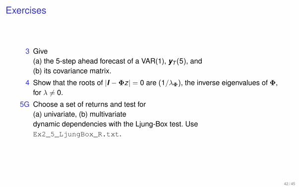
3 Give(a) the 5-step ahead forecast of a VAR(1), yT (5), and(b) its covariance matrix.

4 Show that the roots of |I −Φz| = 0 are (1/λΦ), the inverse eigenvalues of Φ,for λ = 0.

5G Choose a set of returns and test for(a) univariate, (b) multivariatedynamic dependencies with the Ljung-Box test. UseEx2_5_LjungBox_R.txt.

42 / 45

Exercises

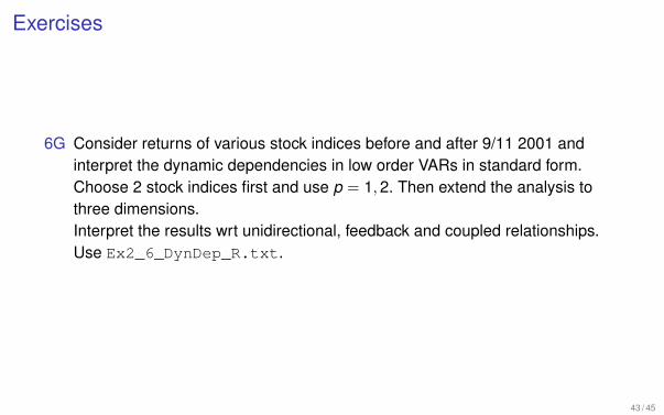
6G Consider returns of various stock indices before and after 9/11 2001 andinterpret the dynamic dependencies in low order VARs in standard form.Choose 2 stock indices first and use p = 1,2. Then extend the analysis tothree dimensions.Interpret the results wrt unidirectional, feedback and coupled relationships.Use Ex2_6_DynDep_R.txt.

43 / 45

Exercises

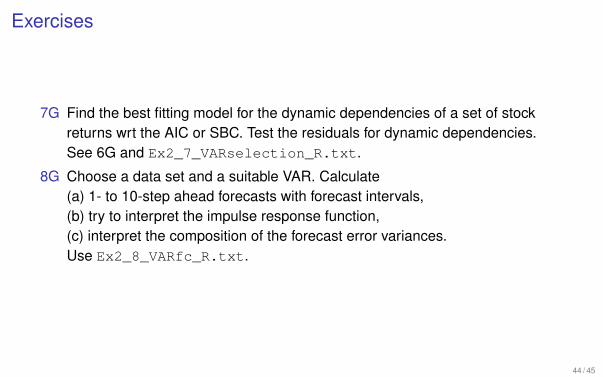
7G Find the best fitting model for the dynamic dependencies of a set of stockreturns wrt the AIC or SBC. Test the residuals for dynamic dependencies.See 6G and Ex2_7_VARselection_R.txt.

8G Choose a data set and a suitable VAR. Calculate(a) 1- to 10-step ahead forecasts with forecast intervals,(b) try to interpret the impulse response function,(c) interpret the composition of the forecast error variances.Use Ex2_8_VARfc_R.txt.

44 / 45

References

Tsay 8.1-2Christopher A. Sims(1980), Macroeconomics and Reality, Econometrica 48

45 / 45