Embed Size (px)
Citation preview

HAL Id: hal-00686444https://hal.archives-ouvertes.fr/hal-00686444v2
Submitted on 15 Oct 2012
HAL is a multi-disciplinary open accessarchive for the deposit and dissemination of sci-entific research documents, whether they are pub-lished or not. The documents may come fromteaching and research institutions in France orabroad, or from public or private research centers.
L’archive ouverte pluridisciplinaire HAL, estdestinée au dépôt et à la diffusion de documentsscientifiques de niveau recherche, publiés ou non,émanant des établissements d’enseignement et derecherche français ou étrangers, des laboratoirespublics ou privés.
Vector Addition Systems with States vs. Petri NetsFlorent Avellaneda, Rémi Morin
To cite this version:Florent Avellaneda, Rémi Morin. Vector Addition Systems with States vs. Petri Nets. 2012. <hal-00686444v2>

Second version: October 13, 2012, 10:36
Vector Addition Systems with States vs. Petri Nets
Florent Avellaneda and Remi Morin
Universite d’Aix-Marseille — CNRS, UMR 7279Laboratoire d’Informatique Fondamentale de Marseille
163, avenue de Luminy, F-13288 Marseille Cedex 9, France
Abstract. Petri nets are a well-known and intensively studied model of concurrency often used tospecify distributed or parallel systems. Vector addition systems with states are simply Petri netsprovided control states. In this paper we introduce a natural partial order semantics for vectoraddition systems with states which extends the process semantics of Petri nets. The addition of controlstates to Petri nets leads to undecidable problems, namely the equality of two process languages givenby two systems. However we show that basic problems about the set of markings reached along theprocesses of a VASS, such as boundedness, covering and reachability, can be reduced to the analogousproblems for Petri nets. We show also how to check effectively any MSO property of these partialorders, provided that the system is bounded. This result generalizes known results and techniquesfor the model checking of compositional message sequence graphs.
Introduction
Consider a set of reactions that take place among a collection of particles such that eachreaction consumes a multiset of available particles and produces a linear combination ofother particle types. This kind of framework can be formalized by a vector addition system[22] or, equivalently, a (pure) Petri net [30]. Consider in addition some control state whichdetermines whether a reaction can occur or not, and such that the occurrence of a reac-tion leads to a possibly distinct control state. Then the model becomes formally a vectoraddition system with states (a VASS), a notion introduced in [21]. It is well-known thatall these models are computationally equivalent, because they can simulate each other [30,33, 34]. More precisely any vector addition system with states over n places can be sim-ulated by some vector addition system over n + 3 places [21]. These simulations do notpreserve strictly the set of reachable markings because they require additional places toencode control states. Still they allow us to use techniques or tools designed for Petri netsto check the properties of the set of reachable markings of a VASS. The addition of controlstates to vector addition systems makes it easier to model and to analyse distributed orparallel systems. For instance it is convenient to use a vector of control states to check thestructural properties of channels within a network of communicating finite state machines[24].
The popular model of message sequence graphs (MSGs) can be regarded as a partic-ular case of VASSs where the only allowed reactions are the sending and the receipt ofone message from one site to another [2, 3, 13, 18, 26]. Then each sequence of reactions canbe described by a partial order of events called a message sequence chart (MSC). EachMSC corresponds to several sequences of elementary actions which are equivalent up tothe reordering of independent events. Similarly each sequence of MSCs is equivalent to
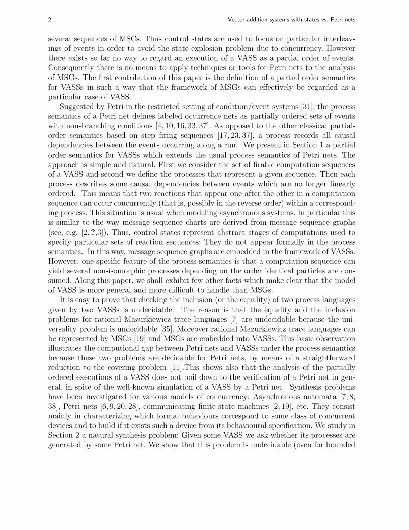
2 Vector addition systems with states vs. Petri nets
several sequences of MSCs. Thus control states are used to focus on particular interleav-ings of events in order to avoid the state explosion problem due to concurrency. Howeverthere exists so far no way to regard an execution of a VASS as a partial order of events.Consequently there is no means to apply techniques or tools for Petri nets to the analysisof MSGs. The first contribution of this paper is the definition of a partial order semanticsfor VASSs in such a way that the framework of MSGs can effectively be regarded as aparticular case of VASS.
Suggested by Petri in the restricted setting of condition/event systems [31], the processsemantics of a Petri net defines labeled occurrence nets as partially ordered sets of eventswith non-branching conditions [4, 10, 16, 33, 37]. As opposed to the other classical partial-order semantics based on step firing sequences [17, 23, 37], a process records all causaldependencies between the events occurring along a run. We present in Section 1 a partialorder semantics for VASSs which extends the usual process semantics of Petri nets. Theapproach is simple and natural. First we consider the set of firable computation sequencesof a VASS and second we define the processes that represent a given sequence. Then eachprocess describes some causal dependencies between events which are no longer linearlyordered. This means that two reactions that appear one after the other in a computationsequence can occur concurrently (that is, possibly in the reverse order) within a correspond-ing process. This situation is usual when modeling asynchronous systems. In particular thisis similar to the way message sequence charts are derived from message sequence graphs(see, e.g. [2,?,3]). Thus, control states represent abstract stages of computations used tospecify particular sets of reaction sequences: They do not appear formally in the processsemantics. In this way, message sequence graphs are embedded in the framework of VASSs.However, one specific feature of the process semantics is that a computation sequence canyield several non-isomorphic processes depending on the order identical particles are con-sumed. Along this paper, we shall exhibit few other facts which make clear that the modelof VASS is more general and more difficult to handle than MSGs.
It is easy to prove that checking the inclusion (or the equality) of two process languagesgiven by two VASSs is undecidable. The reason is that the equality and the inclusionproblems for rational Mazurkiewicz trace languages [7] are undecidable because the uni-versality problem is undecidable [35]. Moreover rational Mazurkiewicz trace languages canbe represented by MSGs [19] and MSGs are embedded into VASSs. This basic observationillustrates the computional gap between Petri nets and VASSs under the process semanticsbecause these two problems are decidable for Petri nets, by means of a straightforwardreduction to the covering problem [11].This shows also that the analysis of the partiallyordered executions of a VASS does not boil down to the verification of a Petri net in gen-eral, in spite of the well-known simulation of a VASS by a Petri net. Synthesis problemshave been investigated for various models of concurrency: Asynchronous automata [7, 8,38], Petri nets [6, 9, 20, 28], communicating finite-state machines [2, 19], etc. They consistmainly in characterizing which formal behaviours correspond to some class of concurrentdevices and to build if it exists such a device from its behavioural specification. We study inSection 2 a natural synthesis problem: Given some VASS we ask whether its processes aregenerated by some Petri net. We show that this problem is undecidable (even for bounded
Vector addition systems with states vs. Petri nets 3
systems) by means of a reduction to the universality problem for rational Mazurkiewicztrace languages. However we present in the rest of this paper several techniques to checkproperties of a VASS under the process semantics with the help of known algorithms andtools.
A key verification problem for MSGs is to detect channel divergence, i.e. to decidewhether the number of pending messages along an execution is unbounded [2,?,3, 19].This problem is NP-complete. An equivalent problem in the more general setting of VASSsis the prefix-boundedness problem. It consists in checking that the set of markings reachedby prefixes of processes is finite. We present in Section 3 a technique to solve this problemby means of a new construction. We obtain that prefix-boundedness is computationallyequivalent to the boundedness problem for Petri nets and requires exponential space [11].This result exhibits an interesting complexity gap between MSGs and VASSs. It shows thatalgorithms to check properties of MSGs need to be revised in order to deal with the moreexpressive framework of VASSs. Other basic decision problems for the markings reachedby prefixes are of course interesting. We show in particular that the reachability and thecovering of a given marking by prefixes can be solved using the same technique.
The model-checking problem for MSGs against monadic second-order logic (MSO) wasinvestigated first in [25]. As opposed to earlier works [2], formulas are interpreted on thepartially ordered scenarios accepted by the MSGs. This problem was proved decidablefor the whole class of safe MSGs [26] (see also [13]). Each safe MSG can be regarded asa bounded VASS. However a safe MSG can describe an infinite set of markings becausethe reordering of events can produce an unbounded number of pending messages withinchannels: In other words, a safe MSG may be divergent. We present in Section 4 a techniqueto check effectively that all processes of a given bounded VASS satisfy a given MSO formula.We shall explain in details why this result subsumes, but cannot be reduced to, previousworks on the model-checking of MSGs.
1 Model and semantics
The goal of this section is to extend the usual process semantics from Petri nets to VASSs.In order to avoid repetitive definitions we introduce the model of Petri nets with statesas a minimal framework which includes both Petri nets and VASSs. Thus Petri nets areregarded as Petri nets with states provided with a single state whereas VASSs are simplyPetri nets with states using pure transition rules, only. Next we present the notions offirable computation sequence, reachable marking, and (non-branching) process as simplegeneralizations of the classical definitions in the restricted setting of Petri nets.
For simplicity’s sake, for any mapping λ : A→ B between two finite sets A and B, weshall denote also by λ the natural mapping λ : A⋆ → B⋆ from words over A to words overB and the mapping λ : NA → NB from multisets over A to multisets over B such thatλ(µ) =
∑a∈A µ(a) · λ(a) for each multiset µ ∈ NA. Moreover we will often identify a set S
with the multiset µS for which µS(x) = 1 if x ∈ S and µS(x) = 0 otherwise.
4 Vector addition systems with states vs. Petri nets
ı
x + y
q
p : x ➝ x + zc : y + z ➝ y
x
p
x
z
y
c
y
p
x
z c
y
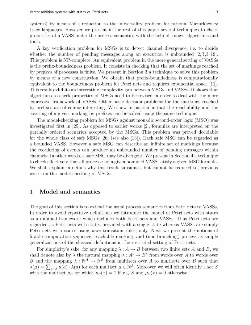
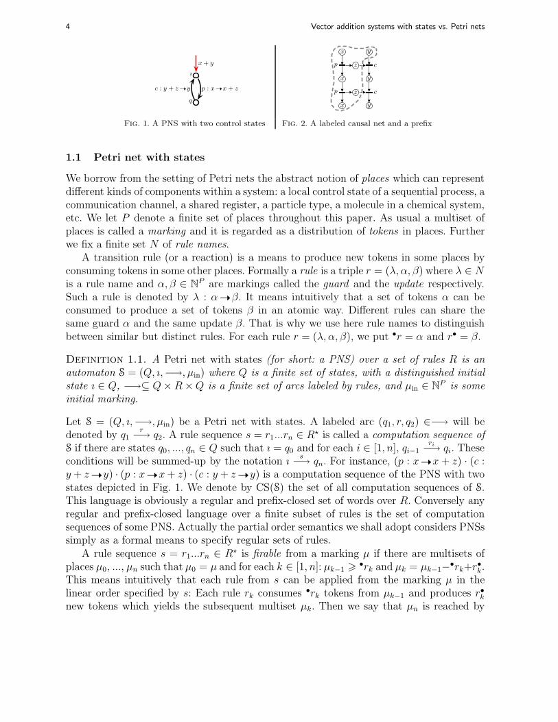
Fig. 1. A PNS with two control states Fig. 2. A labeled causal net and a prefix
1.1 Petri net with states
We borrow from the setting of Petri nets the abstract notion of places which can representdifferent kinds of components within a system: a local control state of a sequential process, acommunication channel, a shared register, a particle type, a molecule in a chemical system,etc. We let P denote a finite set of places throughout this paper. As usual a multiset ofplaces is called a marking and it is regarded as a distribution of tokens in places. Furtherwe fix a finite set N of rule names.
A transition rule (or a reaction) is a means to produce new tokens in some places byconsuming tokens in some other places. Formally a rule is a triple r = (λ, α, β) where λ ∈ Nis a rule name and α, β ∈ NP are markings called the guard and the update respectively.Such a rule is denoted by λ : α ➝ β. It means intuitively that a set of tokens α can beconsumed to produce a set of tokens β in an atomic way. Different rules can share thesame guard α and the same update β. That is why we use here rule names to distinguishbetween similar but distinct rules. For each rule r = (λ, α, β), we put •r = α and r• = β.
Definition 1.1. A Petri net with states (for short: a PNS) over a set of rules R is anautomaton S = (Q, ı,−→, µin) where Q is a finite set of states, with a distinguished initialstate ı ∈ Q, −→⊆ Q×R×Q is a finite set of arcs labeled by rules, and µin ∈ NP is someinitial marking.
Let S = (Q, ı,−→, µin) be a Petri net with states. A labeled arc (q1, r, q2) ∈−→ will bedenoted by q1
r−→ q2. A rule sequence s = r1...rn ∈ R⋆ is called a computation sequence of
S if there are states q0, ..., qn ∈ Q such that ı = q0 and for each i ∈ [1, n], qi−1ri−→ qi. These
conditions will be summed-up by the notation ıs
−→ qn. For instance, (p : x ➝ x + z) · (c :y + z ➝ y) · (p : x ➝ x+ z) · (c : y + z ➝ y) is a computation sequence of the PNS with twostates depicted in Fig. 1. We denote by CS(S) the set of all computation sequences of S.This language is obviously a regular and prefix-closed set of words over R. Conversely anyregular and prefix-closed language over a finite subset of rules is the set of computationsequences of some PNS. Actually the partial order semantics we shall adopt considers PNSssimply as a formal means to specify regular sets of rules.
A rule sequence s = r1...rn ∈ R⋆ is firable from a marking µ if there are multisets ofplaces µ0, ..., µn such that µ0 = µ and for each k ∈ [1, n]: µk−1 > •rk and µk = µk−1−
•rk+r•k.
This means intuitively that each rule from s can be applied from the marking µ in thelinear order specified by s: Each rule rk consumes •rk tokens from µk−1 and produces r•knew tokens which yields the subsequent multiset µk. Then we say that µn is reached by
Vector addition systems with states vs. Petri nets 5
the rule sequence s from the marking µ. We also say that s leads to µn. We denote byFCS(S) the set of all firable computation sequences of S. A marking is reachable in S if itis reached by a firable computation sequence of S. A PNS is said to be bounded if the setof its reachable markings is finite.
1.2 VASS, Petri net and causal net
Originally introduced in [21], the notion of a vector addition system with states (for short:a VASS) can be formally defined in several slightly different ways. In this paper, a VASS issimply a PNS such that each rule r labeling an arc is pure, which means that for all placesp ∈ P , •r(p) × r•(p) = 0. This amounts to require that •r(p) > 1 implies r•(p) = 0 andvice versa. For this reason each rule r in a VASS can be represented by a vector v ∈ ZP
where v(p) = r•(p) − •r(p) for all p ∈ P . We could also require that a VASS uses a singlerule name, i.e. for all rules r1, r2 ∈ R, r1
• − •r1 = r2• − •r2 implies r1 = r2. In this way any
two similar rules must carry the same rule name. This restriction would have no effect onthe results presented in this paper.
We explain at present why we can identify the well-known formalism of Petri nets asparticular PNSs provided with a single state.
Definition 1.2. A Petri net is a quadruple N = (P, T,W, µin) where
– P is a finite set of places and T is a finite set of transitions such that P ∩ T = ∅;– W is a map from (P × T ) ∪ (T × P ) to N, called the weight function;
– µin is a map from P to N, called the initial marking.
We shall depict Petri nets in the usual way as in Fig. 4: Black rectangles represent transi-tions whereas circles represent places; moreover tokens in places describe the initial mark-ing. Given a Petri net N = (P, T,W, µin) and a transition t ∈ T , •t =
∑p∈P W (p, t) · p is
the pre-multiset of t and t• =∑
p∈P W (t, p) · p is the post-multiset of t. Similarly we put•p =
∑t∈T W (t, p) · t and p• =
∑t∈T W (p, t) · t for each place p ∈ P .
Let N = (P, T,W, µin) be a Petri net. We will regard N as a PNS SN with the sameset of places P and the same initial marking. Moreover SN is provided with a single stateı such that each transition t ∈ T is represented by a self-loop labeled arc ı
r−→ ı where
r = (t, •t, t•). In this way, the class of Petri nets is faithfully embedded into the subclass ofPNSs provided with a single state such that each transition carries a rule with a distinctrule name. Conversely, take any PNS S with a single state ı such that each transitioncarries a rule with a distinct rule name. The corresponding Petri net shares with S its setof places and its initial marking. Moreover for each self-loop ı
r−→ ı it admits a transition
tr such that •tr = •r and tr• = r•. For instance the PNS from Fig. 3 corresponds to the
Petri net from Fig. 4.
If the weight function W takes only binary values then it is often described as a flowrelation F ⊆ (P × T ) ∪ (T × P ) where (x, y) ∈ F if W (x, y) = 1. Further F+ denotes thetransitive closure of F .

6 Vector addition systems with states vs. Petri nets
x + y
p : x ➝ x + zc : y + z ➝ y
x p z c y
Fig. 3. A PNS with a single state Fig. 4. and the corresponding Petri net
Definition 1.3. [10, 37] A causal net is a Petri net K = (B,E, F, µmin) whose placesare called conditions, whose transitions are called events, and whose weight function takesvalues in {0, 1} and is represented by a flow relation F ⊆ (B×E)∪ (E×B) which satisfiesthe following requirements:
1. the net is acyclic, i.e. for all x, y ∈ B ∪E, (x, y) ∈ F+ implies (y, x) /∈ F+.2. the conditions do not branch, i.e. |•b| 6 1 and |b•| 6 1 for all b ∈ B.3. µmin(b) = 1 if •b = ∅ and µmin(b) = 0 otherwise.
Note that the third requirement guarantees that the initial marking µmin can be recoveredfrom the structure (B,E, F ) because it coincides with the set of minimal conditions. Forthat reason causal nets are often defined as a triple (B,E, F ) satisfying the two firstconditions of Def. 1.3. In the literature causal nets are also called occurrence nets, see e.g.[4, 14, 16, 15, 33]. However more general Petri nets are called occurrence nets in the theoryof partial unfolding or branching processes [10, 12, 29].
The transitive and reflexive closure F ∗ of the flow relation F in a causal net K =(B,E, F, µmin) yields a partial order over the set of events E. A configuration is a subsetof events H ⊆ E that is downwards closed, i.e. e′F ∗e and e ∈ H imply e′ ∈ H . Eachconfiguration H defines a prefix causal net KH whose events are precisely the events fromH and whose places consists of the minimal places of K (with respect to the partial orderrelation F ∗) and all places related to some event from H . For instance Fig. 2 exhibits asubset of a causal net (circled with a dotted line) that is a prefix of that causal net. Foreach class of labeled causal nets L, we denote by Pref(L) the class of all prefixes of alllabeled causal nets from L.
1.3 Simulation of a VASS by a Petri net
Let us now recall how a k-dimensional VASS or more generally a PNS S with k places canbe simulated by a Petri net N with k+n places, where n is the number of states [34, 30]. Theusual construction is illustrated by Fig. 5 which shows on the left-hand side a PNS with 2states (ı and q) and 3 places (x, y and z) and on the right-hand side the corresponding Petrinet with 5 places: Each place from S and each state from S corresponds to a place from N.The initial marking of N describes the initial marking of S and some token is added in theplace corresponding to the initial state of S. Moreover each arc q1
r−→ q2 in S is represented
by a transition in N. It is easy to see that there is a one-to-one correspondence betweenthe firable computation sequences of S and the firable rule sequences of N; moreover themarking reached by N describes the marking reached by S and the current state of S.
This construction of N from S is interesting because it enables us to analyse the setof reachable markings of S by means of usual techniques from the Petri net literature (see

Vector addition systems with states vs. Petri nets 7
ı
x + y
q
p : x ➝ x + zc : y + z ➝ y ;
x
z
y
p
c
ı
q
Fig. 5. Simulation of a PNS by a Petri net
[11] for a survey). In particular the boundedness problem asks whether the set of reachablemarkings is finite whereas the covering problem asks whether a given marking µ is coveredby some reachable marking µ′, i.e. µ 6 µ′. These two problems are decidable (for Petrinets and Petri nets with states) but they can require exponential space [32].
The simulation of a PNS by a Petri net leads us to the next result.
Proposition 1.4. Let S be a PNS and r be a rule attached to some arc of S. We candecide whether r occurs in a firable computation sequence of S.
Proof. We have recalled that there is a one-to-one correspondence between the firablecomputation sequences of S and the firable computation sequences of N. The rule r occursin a firable computation sequence of S if and only if a corresponding transition t in N occursin a firable transition sequence in N. This is equivalent to check whether the marking of•t is covered by a reachable marking of N. As mentionned above this question is known tobe decidable.
1.4 Process semantics of a PNS
In this paper we are interested in a semantics of PNS based on causal nets which is adirect generalization of the process semantics of Petri nets [4, 10, 15, 16, 33, 37]. The processsemantics of Petri nets characterizes the labeled causal nets that describe an execution ofa given Petri net. We have already observed that each transition of a Petri net can beregarded as a rule. For that reason we adopt a graphical representation of rules similar toa transition of a Petri net, as depicted in Fig. 6. Given an initial multiset of places, eachfirable computation sequence can be represented by a causal net, called a process, whichsomehow glues together the representations of each rule. For instance the labeled causalnet K from Fig. 2 depicts a process of the Petri net N from Fig. 4 in which each conditionof K is labeled by a place of N and each event of K is labeled by a transition of N.
The following definition explains how processes are derived from a given rule sequence.Next the processes of a PNS will be defined as the processes of its firable computationsequences (Def. 1.6).
Definition 1.5. A process of a rule sequence s = r1...rn ∈ R⋆ from a marking µ ∈ NP
consists of a causal net K = (B,E, F, µmin) with n events e1, ..., en provided with a labelingπ : B ∪E → P ∪N such that the following conditions are satisfied:
1. π(b) ∈ P for all b ∈ B, π(e) ∈ N for all e ∈ E, and π(µmin) = µ;

8 Vector addition systems with states vs. Petri nets
x y
a
x z z
x yz
p
x
z c
y
p
x
z c
y
x yz
p
x
z c
y
p
x
z c
y
Fig. 6. Rule a : x + y ➝ x + 2z Fig. 7. Two processes from x + y + z
2. ri = (π(ei), π(•ei), π(ei•)) for all i ∈ [1, n];
3. eiF+ej implies i < j for any two i, j ∈ [1, n].
We denote by [[s]]µ the class of all processes of s from µ.
In this definition the mapping π denotes the labeling of K and its natural extension tomultisets. The first condition asserts that the initial marking of the causal net describesthe marking µ; moreover each condition is associated with some place and each eventcorresponds to some rule name. The second condition requires that the label, the pre-set and the post-set of each event coincide with the name, the guard and the update ofthe corresponding rule. Finally the last property ensures that the total order of rules ins corresponds to an order extension of the partial order of events in K. Consequentlyany subset of events {e1, ..., ek} is downwards closed. Moreover the prefix causal net K′
corresponding to the configuration {e1, ..., en−1} is a process of the rule sequence r1...rn−1
from the same marking µ. Consequently the class of processes of a rule sequence couldbe also defined inductively over its length, as we will see in Prop. 3.3. Furthermore it iseasy to see that the class of processes of a rule sequence is empty if and only if the rulesequence is not firable from µmin.
Let H be a configuration of a process K = (B,E, F, µmin, π) of a rule sequence s fromµ. Let Bmax be the set of maximal conditions of the prefix KH w.r.t. F ∗. Then the multisetof places π(Bmax) is called the marking reached by KH and we say that KH leads to themarking π(Bmax). Let sH be a linear extension of the events from H . Then it is clear thatthe rule sequence π(sH) is firable from µ and leads to the marking π(Bmax); moreover KH
is a process of π(sH) from µ.
Roughly speaking, any labeled causal net isomorphic to a process of s is also a processof s. In particular the class of processes of the empty rule sequence from some marking µcollects all labeled causal nets with no event and such that its set of labeled places representsthe multiset µ. Further a rule sequence may give rise to multiple (non-isomorphic) causalnets depending on the consumption of tokens by each event and the initial marking. Forinstance the computation sequence (p : x ➝ x+z)·(c : y+z ➝ y)·(p : x ➝ x+z)·(c : y+z ➝ y)of the PNS from Fig. 1 corresponds to the causal net from Fig. 2. However if there arex + y + z tokens initially, then this computation sequence corresponds to the two labeledcausal nets from Fig. 7 among some others.
Definition 1.6. Let S be a PNS with initial marking µin. A process of S is a process ofa computation sequence of S from µin. We let [[S]] denote the class of all processes of S.

Vector addition systems with states vs. Petri nets 9
Thus [[S]] =⋃
s∈CS(S) [[s]]µin. It is easy to check that the processes of a PNS provided with
a single state are precisely the processes of the corresponding Petri net w.r.t. the usualprocess semantics [4, 15, 37]. Moreover any prefix of a process of S is a process of somerule sequence. Consequently the class of processes of a Petri net is closed by prefixes.However the set of processes of a PNS need not to be prefix-closed in general, as the nextexample shows.
Example 1.7. Consider the PNS from Fig. 1 with initial marking x + y and its processdepicted in Fig. 2. Clearly the prefix of this process circled with the dotted line in Fig. 2is not a process of that PNS.
A PNS is said to be prefix-bounded if the set of markings reached by prefixes is finite.Clearly any prefix-bounded PNS is bounded. The converse property does not hold in gen-eral. Continuing Example 1.7, each process of the PNS from Fig. 1 leads to a marking withat most 3 tokens whereas prefixes of these processes lead to infinitely many distinct mark-ings (see in Fig. 2 a prefix of a process which leads to a marking with 4 tokens). Howeverwe stress that each bounded Petri net is prefix-bounded because its class of processes isprefix-closed.
Note that the simulation of a PNS by a Petri net considered in Subsection 1.3 is notfaithful from the partial order point-of-view we adopt here. Consider again Figure 5. Theprocesses of the PNS S (with three places) on the left-hand side differ from the processesof the Petri net N (with five places) on the right-hand side. In Section 3 we introduce asimulation of a PNS by another PNS that allows us to analyse the set of markings reachedalong the prefixes of the processes of a given PNS.
1.5 From compositional MSGs to PNSs
The formalism of compositional message sequence graphs (cMSGs) was introduced in [18]in order to strengthen the expressive power of MSGs and to provide an algebraic frameworkfor the whole class of regular sets of MSCs [19]. As opposed to usual MSGs, cMSGs arebuilt on components MSCs in which unmatched send or receive events are allowed. It wasargued in [18] that simple protocols such as the alternating bit protocol can be describedby cMSGs but not by MSGs. With no surprise cMSGs can be regarded as a particular caseof VASS under the process semantics.
Consider a distributed system consisting of a set I of sites and a set K of communicationchannels between pairs of sites. The behaviour of such a system can be specified by a PNSover the set P = I ∪ K of places such that the sending of a message from site i to sitej within the channel ki,j from i to j is encoded by a rule i ➝ i + ki,j and the receipt ofsuch a message is encoded by a rule j + ki,j ➝ j. Then we require that the initial marking(and each reachable marking) contains a single token in each place i ∈ I so that allevents on a given site are linearly ordered. Such a PNS can actually be regarded as acompositional message sequence graph. The partial order semantics of cMSGs consists ofmessage sequence charts which are simply a partial order of events obtained from a processby removing all conditions.

10 Vector addition systems with states vs. Petri nets
ı
i + j + n · w
q1 q2
q3
i + w ➝ i j + m ➝ j
i ➝ i + m j ➝ j + a
i + a ➝ ii ➝ i + w
Tim
e
i jw
i + w ➝ i
i
i ➝ i + d
i
d j + d ➝ j
j
i + a ➝ i
i
a j ➝ j + a
j
i ➝ i + w
wi
Fig. 8. Sliding window protocol Fig. 9. A process with n = 1
Example 1.8. The PNS from Figure 8 describes a simplified sliding window protocolused to transmit data from a server i to a client j. The maximal number of missingacknowledgments is specified by the n initial tokens in the place w (the window). Thesystem behaviour consists of three basic steps.
1. The server sends a new data formalized by a token d if some token w is available: Itconsumes first a w token: i+ w ➝ i and next sends a new data: i ➝ i+ d.
2. The client receives a data and returns an acknowledgment formalized by a token a: Itconsumes first a data: j + d ➝ j and next produces the ack: j ➝ j + a.
3. The server receives an acknowledgment and increments the window size: First the ackis consumed: i+ a ➝ i and then a new token w is released: i ➝ i+ w.
A typical process of this system with n = 1 is depicted in Figure 9. It is clear that thissystem is bounded and even prefix-bounded.
Since local variables are prohibited in MSGs, the size of any safe cMSG equivalent to thePNS from the above example is exponential in the size of n. Thus a bounded PNS can beexponentially more concise than an equivalent safe cMSG. If this protocol starts with aninitial window size of n = 2k ·w, then any safe cMSG describing the same class of processesneeds 2k distinct states.
2 Checking inclusion properties
A classical issue in concurrency theory consists in characterizing the expressive power ofa model. Then a usual problem is the synthesis of a system from its behavioural specifi-cation. In this section we consider Petri nets with states as a means to specify concurrentbehaviours in the form of processes. We tackle the problem of building a Petri net equiva-lent to some given Petri net with states. Two classes of specifications are studied accordingto the notion of equivalence we adopt.
Definition 2.1. A Petri net with states S is realizable (resp. prefix-realizable) if there issome Petri net N such that [[S]] = [[N]] (resp. Pref([[S]]) = [[N]]).
Note that the Petri net with states S from Figure 1 is not realizable because the setof processes it accepts is not prefix-closed (Example 1.7) whereas the set of processes
Vector addition systems with states vs. Petri nets 11
x + y
a : x ➝ xb : y ➝ y
c : x + y ➝ z
x y
b
y
c
z
Fig. 10. A non prefix-realizable PNS Fig. 11. Some implied process
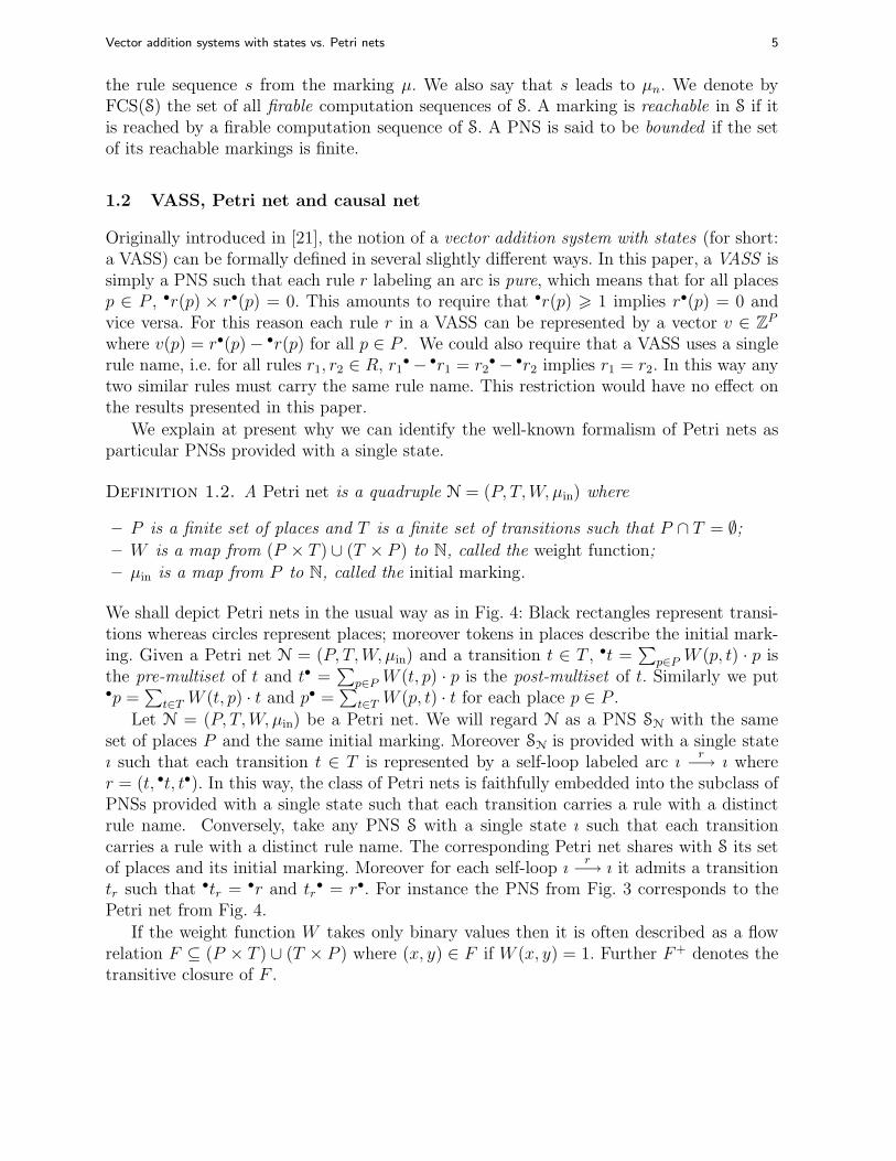
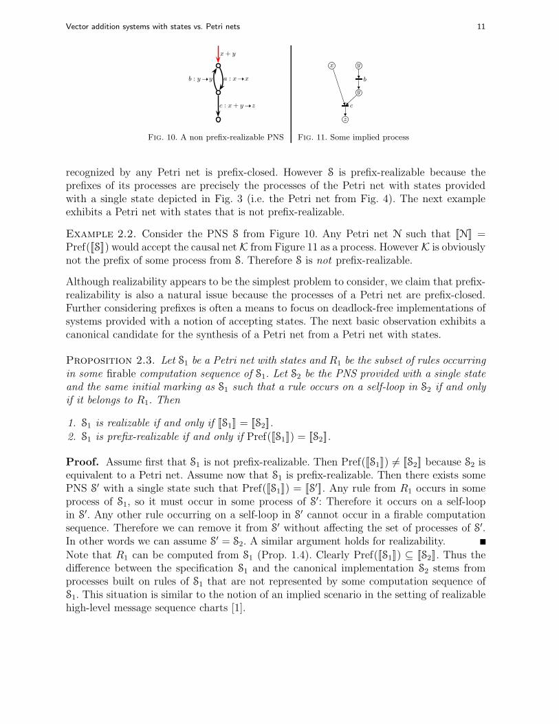
recognized by any Petri net is prefix-closed. However S is prefix-realizable because theprefixes of its processes are precisely the processes of the Petri net with states providedwith a single state depicted in Fig. 3 (i.e. the Petri net from Fig. 4). The next exampleexhibits a Petri net with states that is not prefix-realizable.
Example 2.2. Consider the PNS S from Figure 10. Any Petri net N such that [[N]] =Pref([[S]]) would accept the causal net K from Figure 11 as a process. However K is obviouslynot the prefix of some process from S. Therefore S is not prefix-realizable.
Although realizability appears to be the simplest problem to consider, we claim that prefix-realizability is also a natural issue because the processes of a Petri net are prefix-closed.Further considering prefixes is often a means to focus on deadlock-free implementations ofsystems provided with a notion of accepting states. The next basic observation exhibits acanonical candidate for the synthesis of a Petri net from a Petri net with states.
Proposition 2.3. Let S1 be a Petri net with states and R1 be the subset of rules occurringin some firable computation sequence of S1. Let S2 be the PNS provided with a single stateand the same initial marking as S1 such that a rule occurs on a self-loop in S2 if and onlyif it belongs to R1. Then
1. S1 is realizable if and only if [[S1]] = [[S2]].
2. S1 is prefix-realizable if and only if Pref([[S1]]) = [[S2]].
Proof. Assume first that S1 is not prefix-realizable. Then Pref([[S1]]) 6= [[S2]] because S2 isequivalent to a Petri net. Assume now that S1 is prefix-realizable. Then there exists somePNS S′ with a single state such that Pref([[S1]]) = [[S′]]. Any rule from R1 occurs in someprocess of S1, so it must occur in some process of S′: Therefore it occurs on a self-loopin S′. Any other rule occurring on a self-loop in S′ cannot occur in a firable computationsequence. Therefore we can remove it from S′ without affecting the set of processes of S′.In other words we can assume S′ = S2. A similar argument holds for realizability.
Note that R1 can be computed from S1 (Prop. 1.4). Clearly Pref([[S1]]) ⊆ [[S2]]. Thus thedifference between the specification S1 and the canonical implementation S2 stems fromprocesses built on rules of S1 that are not represented by some computation sequence ofS1. This situation is similar to the notion of an implied scenario in the setting of realizablehigh-level message sequence charts [1].
12 Vector addition systems with states vs. Petri nets
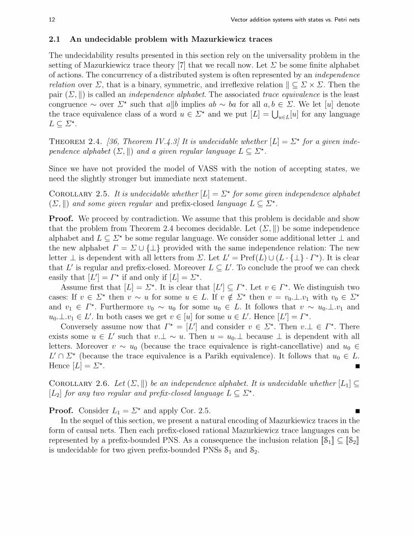
2.1 An undecidable problem with Mazurkiewicz traces
The undecidability results presented in this section rely on the universality problem in thesetting of Mazurkiewicz trace theory [7] that we recall now. Let Σ be some finite alphabetof actions. The concurrency of a distributed system is often represented by an independencerelation over Σ, that is a binary, symmetric, and irreflexive relation ‖ ⊆ Σ ×Σ. Then thepair (Σ, ‖) is called an independence alphabet. The associated trace equivalence is the leastcongruence ∼ over Σ⋆ such that a‖b implies ab ∼ ba for all a, b ∈ Σ. We let [u] denotethe trace equivalence class of a word u ∈ Σ⋆ and we put [L] =
⋃u∈L[u] for any language
L ⊆ Σ⋆.
Theorem 2.4. [36, Theorem IV.4.3] It is undecidable whether [L] = Σ⋆ for a given inde-pendence alphabet (Σ, ‖) and a given regular language L ⊆ Σ⋆.
Since we have not provided the model of VASS with the notion of accepting states, weneed the slightly stronger but immediate next statement.
Corollary 2.5. It is undecidable whether [L] = Σ⋆ for some given independence alphabet(Σ, ‖) and some given regular and prefix-closed language L ⊆ Σ⋆.
Proof. We proceed by contradiction. We assume that this problem is decidable and showthat the problem from Theorem 2.4 becomes decidable. Let (Σ, ‖) be some independencealphabet and L ⊆ Σ⋆ be some regular language. We consider some additional letter ⊥ andthe new alphabet Γ = Σ ∪ {⊥} provided with the same independence relation: The newletter ⊥ is dependent with all letters from Σ. Let L′ = Pref(L) ∪ (L · {⊥} · Γ ⋆). It is clearthat L′ is regular and prefix-closed. Moreover L ⊆ L′. To conclude the proof we can checkeasily that [L′] = Γ ⋆ if and only if [L] = Σ⋆.
Assume first that [L] = Σ⋆. It is clear that [L′] ⊆ Γ ⋆. Let v ∈ Γ ⋆. We distinguish twocases: If v ∈ Σ⋆ then v ∼ u for some u ∈ L. If v /∈ Σ⋆ then v = v0.⊥.v1 with v0 ∈ Σ⋆
and v1 ∈ Γ ⋆. Furthermore v0 ∼ u0 for some u0 ∈ L. It follows that v ∼ u0.⊥.v1 andu0.⊥.v1 ∈ L′. In both cases we get v ∈ [u] for some u ∈ L′. Hence [L′] = Γ ⋆.
Conversely assume now that Γ ⋆ = [L′] and consider v ∈ Σ⋆. Then v.⊥ ∈ Γ ⋆. Thereexists some u ∈ L′ such that v.⊥ ∼ u. Then u = u0.⊥ because ⊥ is dependent with allletters. Moreover v ∼ u0 (because the trace equivalence is right-cancellative) and u0 ∈L′ ∩ Σ⋆ (because the trace equivalence is a Parikh equivalence). It follows that u0 ∈ L.Hence [L] = Σ⋆.
Corollary 2.6. Let (Σ, ‖) be an independence alphabet. It is undecidable whether [L1] ⊆[L2] for any two regular and prefix-closed language L ⊆ Σ⋆.
Proof. Consider L1 = Σ⋆ and apply Cor. 2.5.In the sequel of this section, we present a natural encoding of Mazurkiewicz traces in the
form of causal nets. Then each prefix-closed rational Mazurkiewicz trace languages can berepresented by a prefix-bounded PNS. As a consequence the inclusion relation [[S1]] ⊆ [[S2]]is undecidable for two given prefix-bounded PNSs S1 and S2.
Vector addition systems with states vs. Petri nets 13
x y
a
x
b
y
c
yx
a
x
b
y
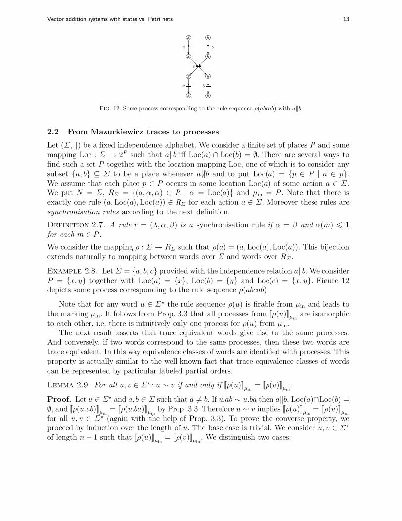
Fig. 12. Some process corresponding to the rule sequence ρ(abcab) with a‖b
2.2 From Mazurkiewicz traces to processes
Let (Σ, ‖) be a fixed independence alphabet. We consider a finite set of places P and somemapping Loc : Σ → 2P such that a‖b iff Loc(a) ∩ Loc(b) = ∅. There are several ways tofind such a set P together with the location mapping Loc, one of which is to consider anysubset {a, b} ⊆ Σ to be a place whenever a6 ‖b and to put Loc(a) = {p ∈ P | a ∈ p}.We assume that each place p ∈ P occurs in some location Loc(a) of some action a ∈ Σ.We put N = Σ, RΣ = {(a, α, α) ∈ R | α = Loc(a)} and µin = P . Note that there isexactly one rule (a,Loc(a),Loc(a)) ∈ RΣ for each action a ∈ Σ. Moreover these rules aresynchronisation rules according to the next definition.
Definition 2.7. A rule r = (λ, α, β) is a synchronisation rule if α = β and α(m) 6 1for each m ∈ P .
We consider the mapping ρ : Σ → RΣ such that ρ(a) = (a,Loc(a),Loc(a)). This bijectionextends naturally to mapping between words over Σ and words over RΣ .
Example 2.8. Let Σ = {a, b, c} provided with the independence relation a‖b. We considerP = {x, y} together with Loc(a) = {x}, Loc(b) = {y} and Loc(c) = {x, y}. Figure 12depicts some process corresponding to the rule sequence ρ(abcab).
Note that for any word u ∈ Σ⋆ the rule sequence ρ(u) is firable from µin and leads tothe marking µin. It follows from Prop. 3.3 that all processes from [[ρ(u)]]µin
are isomorphicto each other, i.e. there is intuitively only one process for ρ(u) from µin.
The next result asserts that trace equivalent words give rise to the same processes.And conversely, if two words correspond to the same processes, then these two words aretrace equivalent. In this way equivalence classes of words are identified with processes. Thisproperty is actually similar to the well-known fact that trace equivalence classes of wordscan be represented by particular labeled partial orders.
Lemma 2.9. For all u, v ∈ Σ⋆: u ∼ v if and only if [[ρ(u)]]µin= [[ρ(v)]]µin
.
Proof. Let u ∈ Σ⋆ and a, b ∈ Σ such that a 6= b. If u.ab ∼ u.ba then a‖b, Loc(a)∩Loc(b) =∅, and [[ρ(u.ab)]]µin
= [[ρ(u.ba)]]µinby Prop. 3.3. Therefore u ∼ v implies [[ρ(u)]]µin
= [[ρ(v)]]µin
for all u, v ∈ Σ⋆ (again with the help of Prop. 3.3). To prove the converse property, weproceed by induction over the length of u. The base case is trivial. We consider u, v ∈ Σ⋆
of length n + 1 such that [[ρ(u)]]µin= [[ρ(v)]]µin
. We distinguish two cases:
14 Vector addition systems with states vs. Petri nets
1. u = u′.a and v = v′.a for some u′, v′ ∈ Σ⋆ and a ∈ Σ. We have ρ(u) = ρ(u′).ρ(a) andρ(v) = ρ(v′).ρ(a). By Prop. 3.3 we have [[ρ(u′)]]µin
= [[ρ(v′)]]µin. It follows from induction
hypothesis that u′ ∼ v′ hence u′.a ∼ v′.a.2. u = u′.a and v = v′.b for some u′, v′ ∈ Σ⋆ and a, b ∈ Σ with a 6= b. We have ρ(u) =ρ(u′).ρ(a) and ρ(v) = ρ(v′).ρ(b) with ρ(a) 6= ρ(b). Then any labeled causal net Kfrom [[ρ(u)]]µin
= [[ρ(v)]]µinincludes two maximal events ea and eb labeled by a and b
respectively. It follows that a‖b. Let K′ be the prefix of K obtained by erasing the twomaximal event ea and eb. We consider a linear extension w′ of the Σ-labeled eventsfrom K′. Then K′ is the process from [[ρ(w′)]]µin
. Moreover [[ρ(w′.a)]]µin= [[ρ(v′)]]µin
and[[ρ(w′.b)]]µin
= [[ρ(u′)]]µin. By induction hypothesis, we get w′.a ∼ v′ and w′.b ∼ u′. On
the other hand w′.ab ∼ w′.ba because a‖b. Hence u ∼ w′.ba ∼ w′.ab ∼ v.
We consider at present a regular and prefix-closed language L ⊆ Σ⋆ and a finite au-tomaton A(L) = (Q, ı,−→A(L)) whose states are all accepting and which recognized L.We may assume that each state of A(L) is reachable from the initial state and each ac-tion of Σ appears on a labeled arc of A(L). We build from the automaton A(L) the PNSS(L) = (Q, ı,−→S(L), µin) with the same set of states Q, the same initial state ı ∈ Q andsuch that for each rule r = (a, α, α) ∈ RΣ and all states q1, q2 ∈ Q, there is some labeledarc q1
r−→S(L) q2 if q1
a−→A(L) q2. Observe here the multiset of tokens is left unchanged by
each rule. Consequently the set of markings reached by prefixes of [[S(L)]] is finite, i.e. thePNS SL is prefix-bounded. For any two regular and prefix-closed languages L1, L2 ⊆ Σ⋆
Lemma 2.9 shows that we have [L1] ⊆ [L2] if and only if [[SL1]] ⊆ [[SL2
]]. Thus the property[[S1]] ⊆ [[S2]] is undecidable for two given prefix-bounded PNS S1 and S2. We can strengthenthis observation by the next statement.
Theorem 2.10. The property [[N]] ⊆ [[S]] is undecidable for a prefix-bounded PNS S anda bounded Petri net N.
Proof. Let L ⊆ Σ⋆ be a regular and prefix-closed language and S(L) be the correspondingPNS. Let N(L) be the Petri net collecting all rules R⋆
Σ of S(L). Then [[N(L)]] = [[R⋆Σ ]].
Moreover we can check that [[S(L)]] = [[R⋆Σ ]] if and only if [L] = Σ⋆.
Assume first that [[S]] = [[R⋆Σ ]]. Let u ∈ Σ⋆. We have [[ρ(u)]]µin
= [[w]]µinfor some
w ∈ CS(S). Let v = ρ−1(w). Clearly v ∈ L. Since [[ρ(u)]]µin= [[ρ(v)]]µin
we get u ∼ v byLemma 2.9. Hence Σ⋆ = [L].
Assume now that [L] = Σ⋆. Let w ∈ R⋆Σ . We have ρ−1(w) ∈ Σ⋆. Then ρ−1(w) ∼ u for
some u ∈ L. It follows from Lemma 2.9 that [[w]]µin= [[ρ(u)]]µin
. Moreover ρ(u) ∈ CS(S).Therefore [[R⋆
Σ ]]µin= [[CS(S)]]µin
.By means of a slightly more involved encoding of Mazurkiewicz traces, we show in the
next section that Theorem 2.10 holds also if S is a prefix-bounded VASS.
2.3 Gap between VASS and Petri nets
At present we focus on the subclass of vector addition systems with states, i.e. Petri netswith states with pure rules only. So far no rule from RΣ is pure, so the processes obtained
Vector addition systems with states vs. Petri nets 15
x y
a
x y
;
x, 0 y, 0
a
x, 1 y, 1
x, 1
x, 0
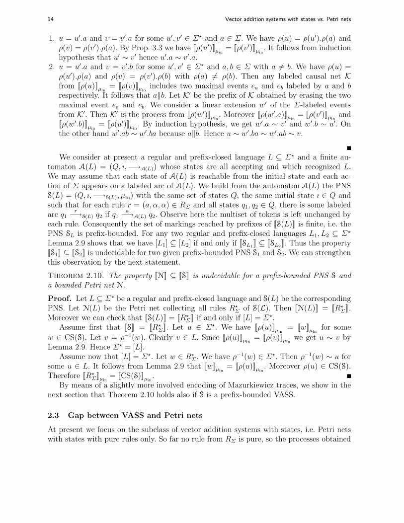
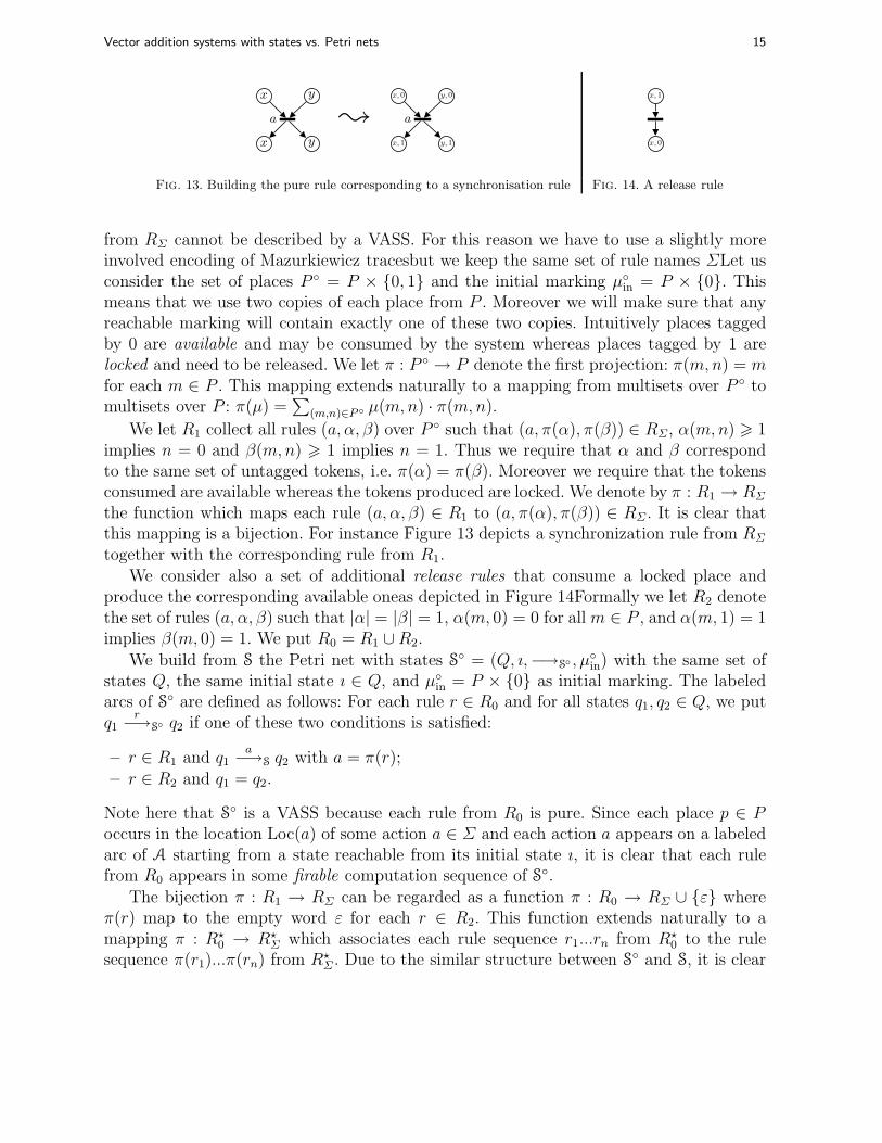
Fig. 13. Building the pure rule corresponding to a synchronisation rule Fig. 14. A release rule
from RΣ cannot be described by a VASS. For this reason we have to use a slightly moreinvolved encoding of Mazurkiewicz tracesbut we keep the same set of rule names ΣLet usconsider the set of places P ◦ = P × {0, 1} and the initial marking µ◦
in = P × {0}. Thismeans that we use two copies of each place from P . Moreover we will make sure that anyreachable marking will contain exactly one of these two copies. Intuitively places taggedby 0 are available and may be consumed by the system whereas places tagged by 1 arelocked and need to be released. We let π : P ◦ → P denote the first projection: π(m,n) = mfor each m ∈ P . This mapping extends naturally to a mapping from multisets over P ◦ tomultisets over P : π(µ) =
∑(m,n)∈P ◦ µ(m,n) · π(m,n).
We let R1 collect all rules (a, α, β) over P ◦ such that (a, π(α), π(β)) ∈ RΣ, α(m,n) > 1implies n = 0 and β(m,n) > 1 implies n = 1. Thus we require that α and β correspondto the same set of untagged tokens, i.e. π(α) = π(β). Moreover we require that the tokensconsumed are available whereas the tokens produced are locked. We denote by π : R1 → RΣ
the function which maps each rule (a, α, β) ∈ R1 to (a, π(α), π(β)) ∈ RΣ . It is clear thatthis mapping is a bijection. For instance Figure 13 depicts a synchronization rule from RΣ
together with the corresponding rule from R1.We consider also a set of additional release rules that consume a locked place and
produce the corresponding available oneas depicted in Figure 14Formally we let R2 denotethe set of rules (a, α, β) such that |α| = |β| = 1, α(m, 0) = 0 for all m ∈ P , and α(m, 1) = 1implies β(m, 0) = 1. We put R0 = R1 ∪R2.
We build from S the Petri net with states S◦ = (Q, ı,−→S◦ , µ◦
in) with the same set ofstates Q, the same initial state ı ∈ Q, and µ◦
in = P × {0} as initial marking. The labeledarcs of S◦ are defined as follows: For each rule r ∈ R0 and for all states q1, q2 ∈ Q, we putq1
r−→S◦ q2 if one of these two conditions is satisfied:
– r ∈ R1 and q1a
−→S q2 with a = π(r);– r ∈ R2 and q1 = q2.
Note here that S◦ is a VASS because each rule from R0 is pure. Since each place p ∈ Poccurs in the location Loc(a) of some action a ∈ Σ and each action a appears on a labeledarc of A starting from a state reachable from its initial state ı, it is clear that each rulefrom R0 appears in some firable computation sequence of S◦.
The bijection π : R1 → RΣ can be regarded as a function π : R0 → RΣ ∪ {ε} whereπ(r) map to the empty word ε for each r ∈ R2. This function extends naturally to amapping π : R⋆
0 → R⋆Σ which associates each rule sequence r1...rn from R⋆
0 to the rulesequence π(r1)...π(rn) from R⋆
Σ . Due to the similar structure between S◦ and S, it is clear

16 Vector addition systems with states vs. Petri nets
that each computation sequence u of S◦ maps to some computation sequence π(u) of S.Furthermore, firable computation sequences correspond to firable computation sequences.Thus we have π : FCS(S◦) → FCS(S). The next observation asserts that the mappingπ : FCS(S◦) → FCS(S) is actually onto.
Proposition 2.11. For all u ∈ FCS(S) there exists u◦ ∈ FCS(S◦) such that π(u◦) = u.
Proof. By an immediate induction over the length of u, we can check that for eachu ∈ FCS(S) there exists some u◦ ∈ FCS(S◦) such that π(u◦) = u and the marking reachedby u◦ is µ◦
in.Recall that each rule of S is a synchronisation rule and the initial marking of S consists ofa single token in each place. As a consequence, for each rule sequence u ∈ R⋆
Σ , the classof processes [[u]]µ◦
inconsists of isomorphic labeled causal nets. For any two rule sequences
u, v ∈ R⋆Σ , we put u ≃ v if [[u]]µ◦
in= [[v]]µ◦
in. Similarly, for each rule sequence u ∈ R⋆
0, the set
of processes [[u]]µ◦
inconsists of isomorphic labeled causal nets because the marking reached
by a firable rule sequence is a set (not a multiset). Moreover we have [[u]]µ◦
in6= ∅ if and only
if the rule sequence u is firable. For any two rule sequences u, v ∈ R⋆0, we put u ≃◦ v if
u = v or [[u]]µ◦
in= [[v]]µ◦
in6= ∅. The second observation ensures that this process equivalence
is preserved by the mapping π : FCS(S◦) → FCS(S).
Proposition 2.12. For all u1, u2 ∈ FCS(S◦), u1 ≃◦ u2 implies π(u1) ≃ π(u2).
Proof. Let u1, u2 ∈ FCS(S◦) be such that u1 ≃◦ u2 and u1 6= u2. Let K be the labeledcausal net from [[u1]]µ◦
in. Then u1 and u2 are two linear extensions of the partial order of
rules occurring in K. We may assume that u1 = v.ab.w and u2 = v.ba.w with v, w ∈ R⋆0
and a, b ∈ R0. We distinguish then two cases.
1. a ∈ R2 or b ∈ R2. Then π(u1) = π(u2) hence π(u1) ≃ π(u2).2. a ∈ R1 and b ∈ R1. Since u1 and u2 are two linear extensions of K, the guards of a andb are disjoint. It follows that π(u1).π(a).π(b) ≃ π(u1).π(b).π(a) hence π(u1) ≃ π(u2).
We will also need the next technical result.
Proposition 2.13. For all firable computation sequences v ∈ FCS(S) and all firable rulesequences u ∈ R⋆
0, if π(u) ≃ v then u ≃◦ w for some firable computation sequence w ∈FCS(S◦).
Proof. We distinguish two cases.
1. The marking reached by u consists of available places only. We consider the rule se-quence w ∈ R0 built inductively over the length of v by replacing each rule r from vby the corresponding rule π−1(r) ∈ R1 followed by a series of release rules from R2
such that all locked places produced by π−1(r) are released. Then w ∈ FCS(S◦) andπ(w) = v. Hence π(u) ≃ π(w). It follows that u ≃◦ w.
2. Some places in the marking reached by u are locked. We add a sequence of release rulesz to u to get w = u.z such that the marking reached by w consists of available placesonly. Then π(w) ≃ v. We apply the first case to get some firable computation sequencew′ ∈ FCS(S◦) such that w ≃◦ w′. We can remove from w′ the release rules of z and getsome firable computation sequence w′′ ∈ FCS(S◦) such that u ≃◦ w′′.
Vector addition systems with states vs. Petri nets 17
Observe here the number of tokens is constant whenever a rule is applied. Consequentlythe set of markings reached by prefixes of [[S◦]] is finite, i.e. S◦ is prefix-bounded. We canprove that S◦ is realizable if and only if S is realizable. Thus,
Theorem 2.14. It is undecidable whether a given prefix-bounded VASS is realizable.
Proof. Let N be the Petri net consisting of all rules of RΣ with the initial markingµin = P . By Prop. 2.3, S is realizable if and only if [[S]] = [[N]]. Moreover N is equivalent toa PNS with only synchronisation rules (and with only one state). We let N◦ be the VASScorresponding to N w.r.t. the above construction of S from S◦. We may apply the threeabove propositions with N and N◦ respectively. Since N◦ has a single state, it is equivalentto a pure Petri net. Further N◦ consists of all rules of R0 and its initial marking is µ◦
in.Since each rule from R0 appears in some firable computation sequence of S◦, Prop. 2.3claims that S◦ is realizable if and only if [[S◦]] = [[N◦]]. We can check that S◦ is realizable ifand only if S is realizable.
Assume first that S◦ is realizable: We have [[S◦]] = [[N◦]]. Let K ∈ [[N]]. Let u be a linearextension of the partial order of rules occurring in K. Then u ∈ FCS(N). There existssome firable computation sequence u◦ ∈ FCS(N◦) such that π(u◦) = u (Prop. 2.11 appliedwith N and N◦). Then u◦ ≃◦ v◦ for some v◦ ∈ FCS(S◦) because [[S◦]] = [[N◦]]. Furthermoreu = π(u◦) ≃ π(v◦) ∈ FCS(S) by Prop. 2.12. Hence K ∈ [[S]]. It follows that [[S]] = [[N]], i.e.S is realizable.
Assume now that S is realizable: We have [[S]] = [[N]]. By construction, [[S◦]] ⊆ [[N◦]].We can check [[N◦]] ⊆ [[S◦]], hence [[N◦]] = [[S◦]] and S◦ is realizable. Let K◦ be a processof N◦ and u◦ be a linear extension of the rules occurring in K◦. Then u◦ ∈ FCS(N◦). Letu = π(u◦). Then u ∈ FCS(N). Since [[S]] = [[N]] we have u ≃ v for some v ∈ FCS(S). ByProp. 2.13, there exists some v◦ ∈ FCS(S◦) such that u◦ ≃◦ v◦. Then K◦ ∈ [[v◦]]µ◦
inhence
K◦ ∈ [[S◦]].Finally we can consider now the problem of prefix-realizability. We call terminating rule
each rule ⊥ : M ➝ ∅ for which M ⊆ P ◦ is a subset of places such that π(M) = P . Wedenote by R3 the set of all terminating rules and we put R⊥ = R0 ∪R3. We build from S◦
the Petri net with states S◦⊥
= (Q, ı,−→S◦
⊥, µ◦
in) with the same set of states Q, the sameinitial state ı ∈ Q, the same set of places P ◦ and the same initial marking µ◦
in. Each labeledarc from S◦ appears in S◦
⊥. For each terminating rule r ∈ R3 and each state q ∈ Q we add
a self-loop qr
−→S◦
⊥q. Then we can check that S◦
⊥is prefix-realizable if and only if S◦ is
realizable. This leads us to the main result of this section.
Theorem 2.15. It is undecidable whether a prefix-bounded VASS is prefix-realizable.
Proof. So far, we have proved that the PNS S is realizable if and only if the VASS S◦ isrealizable. We can prove that S
◦⊥
is prefix-realizable if and only if S◦ is realizable. Assume
first that S◦⊥
is prefix-realizable. Then Pref([[S◦⊥]]) = [[N◦
⊥]] for some Petri net N◦
⊥. Let
N◦ be the Petri net obtained from N◦⊥
by erasing all transitions corresponding to someterminating rule. It is clear that [[S◦]] ⊆ [[N◦]]. To prove that S◦ is realizable, we simplycheck that [[N◦]] ⊆ [[S◦]]. Let K ∈ [[N◦]]. We build the label causal net K⊥ from K by adding

18 Vector addition systems with states vs. Petri nets
an occurrence of some terminating rule ⊥ : M ➝ ∅. This requires that M coincides withthe marking reached by K. Then K⊥ is a process of N◦
⊥. Hence K⊥ ∈ Pref([[S◦
⊥]]). Thus
K⊥ is a prefix of some process K′ ∈ [[u′]]µinwhere u′ ∈ CS(S◦
⊥). Since the terminating rule
⊥ : M ➝ ∅ consumes all places from the marking reached by K, it must be the last ruleof u′, and the single terminating rule of u′, i.e. u′ = u · (⊥ : M ➝ ∅) for some u ∈ CS(S◦).Hence K⊥ = K′. Therefore K ∈ [[u]]µin
and K ∈ [[S◦]].
Assume now that S◦ is realizable. Then [[S◦]] = [[N◦]] for some Petri net N◦. Addingto the Petri net N◦ a transition for each terminating rule yields a new Petri net denotedby N◦
⊥. We can check that [[S◦
⊥]] = [[N◦
⊥]], so S◦
⊥is prefix-realizable. It is clear that [[S◦
⊥]] ⊆
[[N◦⊥]]. Let K ∈ [[N◦
⊥]] and u be a linear extension of the partial order of rules in K. Each
terminating rule ⊥ : M ➝ ∅ may only occur in u as the last rule of u. Let v be the wordobtained by removing the possible occurrence of some terminating rule ⊥ : M ➝ ∅ from u.Then v is a firable rule sequence of N◦ because u is a firable rule sequence of N◦
⊥. Since
[[S◦]] = [[N◦]], we have [[v]]µ◦
in= [[v′]]µ◦
infor some v′ ∈ FCS(S◦). Then [[u]]µ◦
in= [[u′]]µ◦
infor some
u′ ∈ FCS(S◦⊥) obtained from v′ by adding possibly an occurrence some terminating rule.
Therefore K ∈ [[S◦⊥]].
As an immediate consequence, we can now establish the following fact.
Corollary 2.16. Given two prefix-bounded vector addition systems with states S1 and S2,it is undecidable whether [[S1]] = [[S2]] (resp. Pref([[S1]]) = [[S2]], Pref([[S1]]) = Pref([[S2]])).
Proof. By Proposition 2.3, a VASS S is realizable if and only if [[S]] = [[S′]] where S′
is the VASS with a single state which admits a self-loop carrying r if r occurs in somefirable computation sequence of S. By Proposition 1.4, we can effectively build S′ from S.By Theorem 2.14, [[S]] = [[S′]] is undecidable. Therefore [[S1]] = [[S2]] is undecidable for twovector addition systems with states S1 and S2.
Observe now that [[S′]] = Pref([[S′]]). It follows that [[S1]] = Pref([[S2]]) is undecidable fortwo given chemical rule systems S1 and S2.
Finally, S is prefix-realizable if and only if Pref([[S]]) = Pref([[S′]]). It follows fromTheorem 2.15 that Pref([[S1]]) = Pref([[S2]]) is undecidable for two vector addition systemswith states.
The gap between vector addition systems with states and Petri nets is illustrated bythe next result which shows that these decision problems are decidable if one considers(possibly unbounded) Petri nets only.
Proposition 2.17. Let N1 and N2 be two Petri nets. The property [[N1]] ⊆ [[N2]] is decid-able.
Proof. Observe first that this property requires that N1 and N2 share the same initialmarking. Let Ri be the set of rules occurring in some firable computation sequence ofNi. The set Ri can be effectively computed (Prop. 1.4). Then [[N1]] ⊆ [[N2]] if and only ifR1 ⊆ R2.
Vector addition systems with states vs. Petri nets 19
3 Checking reachability properties of process prefixes
Basic decision problems about the set of reachable markings of a Petri net are known to bedecidable, namely boundedness, covering and reachability. Due to the simple simulation ofa VASS by a Petri net recalled in Subsection 1.3 these results apply to the analysis of thereachable markings of a VASS or a PNS.
On the other hand, adopting a partial order semantics leads us to new difficulties andthe model of VASSs is no longer equivalent to Petri nets. For instance the process languageequality [[S1]] = [[S2]] is
– decidable for two Petri nets S1 and S2, because one need simply to compare their initialmarkings and the two subsets of rules occurring in their firable rule sequences.
– undecidable for two prefix-bounded VASSs S1 and S2, because rational sets of Mazurkie-wicz traces can be described by prefix-bounded VASSs.
Thus VASSs and Petri nets are no longer equivalent models under the process semantics.In this section we investigate three basic verification problems about the set of markings
reached by prefixes of processes: boundedness, covering and reachability. We show how toreduce these problems to the particular case of Petri nets in such a way that all complexityand decidability results extend from Petri nets to PNSs under the process semantics.
Definition 3.1. A marking µ is prefix-reachable in a PNS S if there exists a prefix of aprocess of S which leads to the marking µ.
Thus any reachable marking marking is prefix-reachable. In the particular case of Petrinets, conversely, any prefix-reachable marking is reachable, because the class of processesis prefix-closed. However the set of prefix-reachable markings can differ from the set ofreachable markings in general. For instance, each process of the PNS from Fig. 1 leadsto a marking with at most 3 tokens whereas prefixes of these processes lead to infinitelymany distinct markings (see in Fig. 2 a prefix of a process which leads to a marking with4 tokens).
The first basic problem we consider is the prefix-boundedness problem, which askswhether the set of prefix-reachable markings of a given PNS S is finite. We give below alinear construction of a PNS S◦ from S such that S is prefix-bounded if and only if S◦ isbounded. Since the boundedness of S◦ boils down to the boundedness of a Petri net, weget that the prefix-boundedness problem for PNSs is computationally equivalent to theboundedness problem of Petri nets. Further we show that this technique apply to othersimilar basic problems about prefix-reachable markings, namely covering and reachability.
3.1 From Petri nets with states to Petri nets
Let S = (Q, ı,−→, µin) be a fixed PNS. We build a PNS S◦ that allows us to analyse the setof prefix-reachable markings of S. The construction of S◦ from S is illustrated by Fig. 15.The PNS S◦ makes use of three disjoint sets of places: Ppre, Psuf, Pcut which are copies ofthe set of places P of S. We let πpre : P → Ppre, πsuf : P → Psuf, and πcut : P → Pcut be

20 Vector addition systems with states vs. Petri nets
ı
x + y
q
p:x
➝x
+zc
:y
+z
➝y
;
ı
πpre(x) + πpre(y)x : πpre(x) ➝ πsuf(x) + πcut(x)y : πpre(y) ➝ πsuf(y) + πcut(y)z : πpre(z) ➝ πsuf(z) + πcut(z)
q
x : πpre(x) ➝ πsuf(x) + πcut(x)y : πpre(y) ➝ πsuf(y) + πcut(y)z : πpre(z) ➝ πsuf(z) + πcut(z)
p : πpre(x) ➝ πpre(x) + πpre(z)p : πsuf(x) ➝ πsuf(x) + πsuf(z)
c : πpre(y) + πpre(z) ➝ πpre(y)c : πsuf(y) + πsuf(z) ➝ πsuf(y)
Fig. 15. Verification of prefix-reachable markings
the bijections that map each place from P to the corresponding place in Ppre, Pcut and Psuf
respectively. These mappings extend naturally to mappings from multisets to multisets.The initial marking µ◦
in of S◦ is the multiset µ◦in = πpre(µin).
The PNS S◦ shares with S its set of states Q and its initial state ı. It consists of threedisjoint sets of labeled arcs: −→pre,−→suf,−→cut. The restriction of S◦ to the labeled arcsfrom −→pre and to the places from Ppre yields a PNS S
◦pre isomorphic to S. Thus for each
labeled arc q1r
−→ q2 in S with r = (a, •r, r•) there exists some labeled arc q1s
−→pre q2 withs = (a, πpre(
•r), πpre(r•)). Similarly the restriction of S◦ to the labeled arcs from −→suf and
to the places from Psuf yields a PNS S◦suf isomorphic to S, except that its initial marking
is empty: For each labeled arc q1r
−→ q2 in S with r = (a, •r, r•) there exists some labeledarc q1
s−→suf q2 with s = (a, πsuf(
•r), πsuf(r•)). Note that the two PNSs S◦
pre and S◦suf are
synchronized because they share a common set of state. The set of labeled arcs −→cut
consists of a self-loop qs
−→cut q for each state q and each place p ∈ P ; this labeled arcallows to move a token from the place πpre(p) to the place πsuf(p) and to keep track of thattransfer in the place πcut(p), i.e. •s = πpre(p) and s• = πsuf(p) + πcut(p). Note that tokensin Pcut cannot be consumed.
Intuitively, for any process K of S and for any prefix K′ of K, the PNS S◦ can simulatea computation sequence of S which corresponds to K in such a way that each event fromthe prefix K′ corresponds to the occurrence of a labeled arc from −→pre and each eventfrom the suffix K\K′ corresponds to the occurrence of a labeled arc from −→suf. Moreoverthe set of places Pcut keeps track of the tokens transferred from K to K′, i.e. from S◦
pre toS◦
suf, by labeled arcs from −→cut. Thus any prefix-reachable marking of S is representedby the restriction to Ppre ∪ Pcut of some reachable marking of S◦. The key property of thisrepresentation, stated in Prop. 3.2 below, asserts that, conversely, each firable computationsequence of S◦ corresponds to a process K of S and a prefix K′ of K such that the markingof Ppre ∪ Pcut describes the marking reached by K′.
In order to prove our results in details, we shall adopt also the next notations:
– We denote by τpre and τsuf the bijections that maps each labeled arc qr
−→ q′ from S tothe corresponding labeled arc in −→pre and −→suf respectively.
– For each state q ∈ Q, we denote τ qcut the bijection between P and the self-loop labeled
on q from −→cut.
Vector addition systems with states vs. Petri nets 21
In the next statement and the sequel of this section, for each marking µ and for each subsetof places X, we denote by µ|X the restriction of µ to the places from X. The main resultsof this section rely essentially on the next observation.
Proposition 3.2. A multiset of places µ ∈ NP is prefix-reachable in S if and only if thereexists some reachable marking µ◦ of S
◦ such that µ = π−1pre(µ
◦|Ppre) + π−1cut(µ
◦|Pcut).
3.2 Proof of Proposition 3.2
For each rule sequence u = r1...rn ∈ R⋆, the cost of u is the vector cost(u) ∈ ZP suchthat cost(u)(p) =
∑ni=1
•ri(p) − ri•(p) for each p ∈ P . In particular the cost of the empty
rule sequence is the null vector. If a rule sequence u is firable from a marking µ then themarking reached by u from µ is µ− cost(u). Let K be a process of a rule sequence u firablefrom µ. Then µ − cost(u) is the marking reached by K from µ. Moreover the markingµ− cost(u) corresponds to the set of conditions in K that are not input places of any eventin K (which means intuitively that they are still available), i.e. to the maximal places ofK: We have µ− cost(u) =
∑p∈max(K)∩P π(p).
For each rule r such that •r 6 µ − cost(u), we let K · r denote the class of labeledcausal nets obtained by adding to K an event that describes an occurrence of rule r whichconsumes •r available conditions from K.
Proposition 3.3. Let µ ∈ NP . The class of processes of a rule sequence u ∈ R⋆ satisfiesthe three following properties:
– If u is empty, i.e. u = ε, then each process from [[ε]]µ consists of∑
p∈P µ(p) conditionsand no event.
– for all rules r ∈ R, [[u.r]]µ is empty if [[u]]µ is empty or •r µ− cost(u).– for all rules r ∈ R, if [[u]]µ is not empty and •r 6 µ − cost(u) then [[u.r]]µ collects all
processes from K · r for all processes K ∈ [[u]]µ.
Proof. By Definition 1.5, a process of the empty rule sequence from a marking µ consists ofa set of labeled places which represents µ. Consider a rule sequence u and a rule r. Assumethat [[u.r]]µ is not empty. Let K be a labeled causal net from [[u.r]]µ. We have already noticedthat some prefix K′ of K is a process of u from µ. Therefore [[u]]µ is not empty. MoreoverK belongs to K′ · r. Since u.r is a firable rule sequence, •r is smaller than the markingreached by u from µ, i.e. •r 6 µ− cost(u). Thus, if [[u]]µ is empty or •r > µ− cost(u) then[[u.r]]µ is empty. On the other hand, if [[u]]µ is not empty and •r 6 µ − cost(u) then anylabeled causal net from K′ · r where K′ ∈ [[u]]µ is clearly a process of u.r from µ. Furtherany process from [[u.r]]µ can be obtained in this way.
Given two multisets of places µ1, µ2 ∈ NP , the maximum max(µ1, µ2) collects the maximalnumber of tokens in each place: max(µ1, µ2)(p) = max(µ1(p), µ2(p)) for each p ∈ P . Wewill make use of the following requirement function req : R⋆ → NP .
Definition 3.4. The requirement of a rule sequence u ∈ R⋆ is the multiset of placesdefined inductively as follows:

22 Vector addition systems with states vs. Petri nets
– req(ε) = 0,– req(u.a) = max(req(u), •a+ cost(u)) for all u ∈ R⋆ and all a ∈ R.
The next observation shows that the requirement of a rule sequence u is the minimalmarking µ such that u is firable from µ, i.e. [[u]]µ 6= ∅.
Proposition 3.5. Let u ∈ R⋆ and µ ∈ NP . Then [[u]]µ 6= ∅ if and only if µ > req(u).
Proof. We proceed by induction over the length of u. If u = ε then req(u) = 0 henceµ > req(u). Moreover [[ε]]µ contains each labeled causal net with no event and with a setof conditions representing the marking µ. Induction step: Let u ∈ R⋆ and a ∈ R. Assumefirst that [[u.a]]µ 6= ∅. By Prop. 3.3, we have µ > •a+ cost(u). On the other hand, we have[[u]]µ 6= ∅ hence µ > req(u) by induction hypothesis. Thus µ > max(req(u), •a+ cost(u)) =req(u.a). Assume now that [[u.a]]µ = ∅. We distinguish two cases.
1. [[u]]µ = ∅. Then, by induction hypothesis, we have µ < req(u) 6 req(u.a).2. [[u]]µ 6= ∅. Then, by Prop. 3.3, we have µ < •a+ cost(u) 6 max(req(u), •a + cost(u)) =
req(u.a).
Thus [[u.a]]µ 6= ∅ if and only if µ > req(u.a).For each rule sequence u = r1...rn ∈ R⋆ firable from µin, we let µu denote the marking
reached by u from µin, i.e. µu = µin +∑n
i=1(ri•−•ri). Similarly for each transition sequence
s ∈ T ⋆N
firable from the initial marking µ◦in, µ
◦s denotes the marking reached by s in S◦.
We shall use the following notion of partial computation: A partial computation is atriple (u, v, w) ∈ R⋆ × R⋆ × R⋆ such that [[v.w]]µin
∩ [[u]]µin6= ∅ and u ∈ CS(S). Then
[[v]]µin6= ∅ hence the rule sequence v is firable from µin. A partial computation is used as
a witness for a process Ku of u and a prefix Kv of Ku with Kv ∈ [[v]]µin. Note that v need
not to be a prefix of u, nor to be a computation sequence of S. Partial computations areclosely related to prefix-reachable markings, as the next basic observation shows.
Proposition 3.6. For each partial computation (u, v, w), the marking µv is prefix-reachable.Conversely, for any prefix-reachable marking µ, there exists some partial computation(u, v, w) such that µ = µv.
Proof. Let (u, v, w) be a partial computation: There exists some labeled causal net Ksuch that K ∈ [[v.w]]µin
∩ [[u]]µin. By Prop. 3.3, K may be built from a causal net Kv ∈ [[v]]µin
by adding the sequence of rules w, one after the other. Thus Kv is a prefix of K and µv isprefix-reachable.
Let K ∈ [[u]]µinwith u ∈ CS(S) and K′ be a prefix of K. Let v be a linear extension of
the partial order of rules occurring in K′. Then K′ ∈ [[v]]µinand µv is the marking reached
by K′. Let w be a linear extension of the partial order of rules occurring in the suffixK \ K′. Then v.w is a linear extension of the partial order of rules occurring in K henceK ∈ [[v.w]]µin
. Therefore (u, v, w) is a partial computation.
Lemma 3.7. Let (u, v, w) be a partial computation and a ∈ R be a rule such that •a 6 µu.If u.a ∈ CS(S) then (u.a, v, w.a) is a partial computation.

Vector addition systems with states vs. Petri nets 23
Proof. Let K be a labeled causal net from [[v.w]]µin∩ [[u]]µin
. Since •a 6 µu, the class[[u.a]]µin
is not empty (Prop. 3.3). Moreover all causal nets from [[u.a]]µinare obtained from
some causal net from [[u]]µinby adding an occurrence of rule a. In particular we can add
an occurrence of rule a to K and get a causal net from [[u.a]]µin. The latter is also a causal
net from [[v.w.a]]µinsince K ∈ [[v.w]]µin
.
The proof of Prop. 3.2 relies on the two next technical lemmas which can be establishedby means of a bit tedious inductions. The first one asserts that for each firable computationsequence u ∈ FCS(S) and each prefix Kv of each process Ku ∈ [[u]]µin
, the VASS S◦ canbe guided in order to simulate each rule of u in its sequential order so that the markingreached by u is described by the current marking of Ppre ∪ Psuf while the marking reachedby Kv is described by the current marking of Ppre ∪ Pcut. Furthermore we have to makesure that the state q ∈ Q reached by u is also reached by s in S◦ and to check that allevents from Ku that do not occur in Kv are performed by transitions from −→suf. To doso, we have to guide S
◦ to transfer exactly the required number of tokens from Ppre to Psuf,which corresponds to the marking of Pcut.
Lemma 3.8. Let (u, v, w) be a partial computation in S and q be some state such thatı
u−→ q in S. There exists some firable rule sequence s in S◦ which leads to the marking µ◦
s
such that
(a) π−1cut(µ
◦s|Pcut) + π−1
pre(µ◦s|Ppre) = µv,
(b) π−1suf(µ
◦s|Psuf) + π−1
pre(µ◦s|Ppre) = µu,
(c) π−1cut(µ
◦s|Pcut) = req(w),
(d) ıs
−→ q in S◦.
Proof. We proceed by induction over the length of u. If |u| = 0 then u = ε, q = ı,v = ε and w = ε. The empty firing sequence of S◦ satisfies the four above propertiesbecause µ◦
in = πpre(µin). Induction step: We consider some partial computation (u′, v′, w′)
with |u′| = n + 1. We put u′ = u.a with |u| = n and ıu
−→ qa
−→ q′. Let Ku′, Kv′ and Kw′
be three labeled causal nets such that Ku′ ∈ [[u′]]µin∩ [[v′.w′]]µin
, Kv′ ∈ [[v′]]µinis a prefix of
Ku′ and Kw′ ∈ [[w′]]µv′is the corresponding suffix. We know that Ku′ is obtained from some
process Ku ∈ [[u]]µinby adding an event ea that corresponds to an occurrence of rule a. We
distinguish two cases.
1. Event ea occurs in Kw′. Then there is some rule sequence w such that Kw′ ∈ [[w.a]]µv′
and Ku ∈ [[v′.w]]µinso (u, v′, w) is a partial computation of length n. By induction
hypothesis there exists some firable computation sequence s in S◦ such that the fourabove properties are satisfied. In particular, π−1
cut(µ◦s|Pcut) = req(w). Moreover Prop. 3.5
ensures that req(w.a) 6 µv′ because Kw′ ∈ [[w.a]]µv′. Furthermore we have on one
hand π−1cut(µ
◦s|Pcut) = req(w) 6 req(w.a); and on the other hand req(w.a) 6 µv′ i.e.
req(w.a) 6 π−1cut(µ
◦s|Pcut) + π−1
pre(µ◦s|Ppre). Therefore
π−1cut(µ
◦
s|Pcut) 6 req(w.a) 6 π−1cut(µ
◦
s|Pcut) + π−1pre(µ
◦
s|Ppre)
24 Vector addition systems with states vs. Petri nets
It follows that there is some multiset of places µ ∈ NP such that π−1cut(µ
◦s|Pcut) + µ =
req(w.a) with πpre(µ) 6 µ◦s|Ppre. We consider a sequence of transitions A ∈−→⋆
cut inS◦ which consumes the multiset of tokens πpre(µ) and produces the multiset of tokensπsuf(µ). We have
•a+ µv − µu = •a+ cost(w) 6 max(req(w), •a + cost(w)) = req(w.a)
Hence µu − µv + req(w.a) > •a. On the other hand
µu−µv+req(w.a) = µu−µv+π−1cut(µ
◦
s|Pcut)+µ = µu−π−1pre(µ
◦
s|Ppre)+µ = π−1suf(µ
◦
s|Psuf)+µ
Hence π−1suf(µ
◦s.A|Psuf) = π−1
suf(µ◦s|Psuf) + µ > •a. It follows that s.A.τsuf(a) is a firable
computation sequence of S◦. The latter satisfies the required conditions:(a) π−1
pre(µ◦
s.A.τsuf(a)|Ppre) = π−1pre(µ
◦s|Ppre) − µ and π−1
cut(µ◦
s.A.τsuf(a)|Pcut) = π−1cut(µ
◦s|Pcut) + µ
hence π−1pre(µ
◦
s.A.τsuf(a)|Ppre)+π−1cut(µ
◦
s.A.τsuf(a)|Pcut) = π−1pre(µ
◦s|Ppre)+π
−1cut(µ
◦s|Pcut) = µv′ .
(b) π−1pre(µ
◦
s.A.τsuf(a)|Ppre) = π−1pre(µ
◦s|Ppre)−µ, π−1
suf(µ◦
s.A.τsuf(a)|Psuf) = π−1suf(µ
◦s|Psuf)+µ−
•a+
a• therefore π−1pre(µ
◦
s.A.τsuf(a)|Ppre)+π−1suf(µ
◦
s.A.τsuf(a)|Psuf) = π−1pre(µ
◦s|Ppre)+π
−1suf(µ
◦s|Psuf)−
•a + a• = µu.a = µu′.(c) π−1
cut(µ◦
s.A.τsuf(a)|Pcut) = π−1cut(µ
◦s|Pcut) + µ = req(w.a).
(d) ıs
−→ qA
−→ q′′τsuf(a)−→ q′.
2. Event ea occurs in Kv′ . Then there exists some v such that Kv′ ∈ [[v.a]]µinand Ku ∈
[[v.w′]]µin. It follows that (u, v, w′) is a partial computation of length n. By induction
hypothesis, there exists some firable computation sequence s in S◦ such that the four
above properties are satisfied. Then we have
•a 6 µv − req(w′) = π−1cut(µ
◦
s|Pcut) + π−1pre(µ
◦
s|Ppre) − π−1cut(µ
◦
s|Pcut) = π−1pre(µ
◦
s|Ppre).
Therefore τpre(a) can be fired from the marking µ◦s and we get a new firable computation
sequence s.τpre(a). The latter fulfills the required properties.(a) We have π−1
cut(µ◦
s.τpre(a)|Pcut) = π−1cut(µ
◦s|Pcut) and π−1
pre(µ◦
s.τpre(a)|Ppre) = π−1pre(µ
◦s|Ppre) −
•a + a•, hence π−1cut(µ
◦
s.τpre(a)|Pcut) + π−1pre(µ
◦
s.τpre(a)|Ppre) = µv.a.
(b) Since π−1suf(µ
◦
s.τpre(a)|Psuf) = π−1suf(µ
◦s|Psuf) and π−1
pre(µ◦
s.τpre(a)|Ppre) = π−1pre(µ
◦s|Ppre)−
•a+
a• we get π−1suf(µ
◦
s.τpre(a)|Psuf) + π−1pre(µ
◦
s.τpre(a)|Ppre) = µu.a = µu′.
(c) π−1cut(µ
◦
s.τpre(a)|Pcut) = π−1cut(µ
◦s|Pcut) = req(w′).
(d) ıs
−→ qτpre(a)−→ q′.
Lemma 3.9. Let (u, v, w) be a partial computation and a ∈ R be a rule such that •a +req(w) 6 µv. If u.a ∈ CS(S) then (u.a, v.a, w) is a partial computation.
Proof. Let Ku ∈ [[u]]µinand let Kv ∈ [[v]]µin
be a prefix of Ku. Since w is firable fromreq(w), there exists some labeled causal net Kw ∈ [[w]]req(w). We can build a process K′
u
Vector addition systems with states vs. Petri nets 25
of u which admits Kv as prefix and such that the suffix K′u \ Kv corresponds to Kw. In
particular only req(w) tokens from the multiset µv reached by Kv are consumed by Kw.Then we can add an occurrence of rule a to K′
u which consumes •a remaining tokens fromµv − req(w).
Conversely we need to show that the marking of Ppre ∪ Pcut reached after any firabletransition sequence s of S◦ corresponds to a prefix-reachable marking of S, i.e. to somepartial computation (u, v, w). To do so, we have to build a firable rule sequence u ∈ FCS(S),a process Ku ∈ [[u]]µin
and a prefix Kv ∈ [[v]]µininductively from s. At each step the state
reached by s coincides with the state reached by u. When S◦ applies an additional labeledarc a, the corresponding partial computation is either (u, v, w) if a ∈
r−→cut; or (u.r, v, w.r)
if a ∈r
−→suf; or (u.r, v.r, w) if a ∈r
−→pre. In this last case, the rule r and the sequence ofrules w can be performed concurrently: Formally we shall establish that •r+ req(w) 6 µv.This property follows actually from the fact that w can be fired from the marking obtainedby the tokens transferred from Ppre to Psuf, i.e. πcut(req(w)) 6 µ◦
s|Pcut.
Lemma 3.10. Let s be a firable rule sequence in S◦ leading to the state q and the markingµ◦
s. There exists some partial computation (u, v, w) of S such that
(a) π−1cut(µ
◦s|Pcut) + π−1
pre(µ◦s|Ppre) = µv,
(b) π−1suf(µ
◦s|Psuf) + π−1
pre(µ◦s|Ppre) = µu,
(c) π−1cut(µ
◦s|Pcut) > req(w), and
(d) ıu
−→ q in S.
Proof. We proceed by induction over the length of s. If |s| = 0 then s = ε; the empty par-tial computation (ε, ε, ε) satisfies the four requirements because µ◦
in = πpre(µin). Inductionstep: Let s.a be a firable computation sequence of length n + 1. By induction hypothesis,there exists some partial computation (u, v, w) which fulfills the four above requirements.We distinguish three cases:
1. qa
−→cut q in S◦. Then we can check that (u, v, w) satisfies the four requirements for s.a.(a) π−1
cut(µ◦s.a|Pcut) + π−1
pre(µ◦s.a|Ppre) = π−1
cut(µ◦s|Pcut) + π−1
pre(µ◦s|Ppre) = µv.
(b) π−1suf(µ
◦s.a|Psuf) + π−1
pre(µ◦s.a|Ppre) = π−1
suf(µ◦s|Psuf) + π−1
pre(µ◦s|Ppre) = µu.
(c) We have π−1cut(µ
◦s.a|Pcut) > π−1
cut(µ◦s|Pcut) > req(w).
(d) ıu
−→ q by induction hypothesis.2. q
a−→suf q
′. Then τ−1suf
(a) is an arc qr
−→S q′ in S and u.r is a computation sequence of
S. Moreover π−1suf(
•a|Psuf) = •r and π−1suf(a
•|Psuf) = r•. Furthermore •a 6 µ◦s, hence •r 6
π−1suf(µ
◦s|Psuf) 6 µu. By Lemma 3.7 we know that (u.r, v, w.r) is a partial computation
of S. Moreover(a) π−1
cut(µ◦s.a|Pcut) + π−1
pre(µ◦s.a|Ppre) = π−1
cut(µ◦s|Pcut) + π−1
pre(µ◦s|Ppre) = µv.
(b) π−1suf(µ
◦s.a|Psuf) + π−1
pre(µ◦s.a|Ppre) = π−1
suf(µ◦s|Psuf) + π−1
pre(µ◦s|Ppre) + π−1
suf(a• − •a|Psuf) =
µu −•r + r• = µu.r.
(c) We have µs.a|Pcut = µs|Pcut. Moreover •a 6 µ◦s, hence
π−1cut(µ
◦
s|Pcut) > π−1cut(µ
◦
s|Pcut)+π−1suf(
•a−µ◦
s|Psuf) = π−1suf(
•a|Psuf)+(µv−µu) = •r+cost(w)
Then π−1cut(µ
◦s.a|Pcut) = π−1
cut(µ◦s|Pcut) > max(req(w), •r + cost(w)) = req(w.r).
26 Vector addition systems with states vs. Petri nets
(d) ıu
−→ qr
−→ q′ and ıs
−→ qa
−→ q′.
3. qa
−→pre q′. Then τ−1
pre(a) is an arc qr
−→S q′. Moreover π−1
pre(•a|Ppre) = •r and π−1
pre(a•|Ppre) =
r•. We observe first that
(a) π−1cut(µ
◦s.a|Pcut) + π−1
pre(µ◦s.a|Ppre) = µv − π−1
pre(•a|Ppre) + π−1
pre(a•|Ppre) = µv.r
(b) π−1suf(µ
◦s.a|Psuf) + π−1
pre(µ◦s.a|Ppre) = µu − π−1
pre(•a|Ppre) + π−1
pre(a•|Ppre) = µu.r
(c) π−1cut(µ
◦s.a|Pcut) = π−1
cut(µ◦s|Pcut) > req(w)
(d) qr
−→ q′ in S.
Since µ◦s > •a, we have π−1
pre(µ◦s|Ppre) > π−1
pre(•a|Ppre). On the other hand, π−1
cut(µ◦s|Pcut) >
req(w), hence π−1pre(µ
◦s|Ppre)+π−1
cut(µ◦s|Pcut) > π−1
pre(•a|Ppre)+req(w), i.e µv > •r+req(w).
By Lemma 3.9, (u.r, v.r, w) is a partial computation.
We are now ready to prove Prop. 3.2. Let µ be the marking reached by a prefix K′ ofa process K ∈ [[S]]. According to Prop. 3.6, there exists some partial computation (u, v, w)such that µv = µ. By Lemma 3.8, there exists some firable rule sequence s in S◦ such thatπ−1
cut(µ◦s|Pcut) + π−1
pre(µ◦s|Ppre) = µv = µ. Conversely if π−1
cut(µ◦s|Pcut) + π−1
pre(µ◦s|Ppre) = µ for
some firable rule sequence s in S◦ then Lemma 3.10 ensures that there exists some partialcomputation (u, v, w) such that π−1
cut(µ◦s|Pcut) + π−1
pre(µ◦s|Ppre) = µv. Moreover Prop. 3.6
asserts that µv is the marking reached by some prefix K′ of some process K ∈ [[S]].
3.3 Analysis of prefix-reachable markings
At present we make use of the properties of the PNS S◦, in particular Prop. 3.2, in order
to derive some techniques to analyse the set of prefix-reachable markings of S. First, theprefix-boundedness problem asks whether the set of prefix-reachable markings of a givenPNS S is finite. It is easy to prove that the PNS S is prefix-bounded if and only if the PNSS◦ is bounded, which can be checked by means of the usual linear simulation by a Petrinet. Moreover, prefix-boundedness is equivalent to boundedness in the particular case ofPetri nets because the set of processes of a Petri net is closed by prefixes. Thus,
Theorem 3.11. The prefix-boundedness problem of PNSs is computationally equivalent tothe boundedness problem of Petri nets.
Proof. It is clear from Prop. 3.2 that if S◦ is bounded then there are finitely many prefix-reachable markings in S. Conversely, assume that S is prefix-bounded. Then there existssome M ∈ N such that µv(p) 6 M and µu(p) 6 M for all partial computations (u, v, w)of S and all places p ∈ P . Then Lemma 3.10 ensures that if a firable rule sequence of S
◦
leads to some marking µ then µ(p) 6 M for each place p ∈ PS◦ .Second, the prefix-covering problem asks whether a given multiset of places µ ∈ NP iscovered by some prefix-reachable marking µ′ ∈ NP , i.e. µ(p) 6 µ′(p) for all p ∈ P . It iseasy to see that µ is prefix-covered in S if and only if the multiset of places πcut(µ) iscovered by some reachable marking of S
◦. Thus,
Theorem 3.12. The prefix-covering problem for PNSs is computationally equivalent tothe covering problem in Petri nets.
Vector addition systems with states vs. Petri nets 27
Proof. The prefix-covering problem is equivalent to the covering problem in the particularcase of Petri nets. Thus the prefix-covering problem of PNSs is as difficult as the coveringproblem of Petri nets. Moreover checking the coverability of a given marking by the reach-able markings of a PNS can be checked by means of the linear simulation of a PNS by aPetri net. Thus we need simply to show that a marking µ0 is prefix-covered in S if andonly if the multiset of places πcut(µ0) is covered by some reachable marking of S◦.
Let µ0 ∈ NP be a multiset of places. Assume first that µ0 is covered by some prefix-reachable marking µ of S: µ0 6 µ. By Prop. 3.2, there exists some reachable marking µ◦
in S◦ such µ = π−1pre(µ
◦|Ppre) + π−1cut(µ
◦|Pcut). Due to the self-loop labeled arcs from −→cut
in S◦, we can assume that µ◦|Ppre = 0 hence πcut(µ) = µ◦|Pcut and πcut(µ0) 6 µ◦|Pcut.Conversely, assume now that πcut(µ0) 6 µ◦ for some reachable marking µ◦ of S◦. Then,
by Lemma 3.10 and Prop. 3.6, µ0 6 π−1cut(µ
◦|Pcut) 6 µ for some prefix-reachable marking µof S.
Last but not least, the prefix-reachability problem asks whether a given multiset ofplaces is prefix-reachable in S. Let us consider a slight modification S′ of S◦ where for eachplace p ∈ Psuf, each state q ∈ S◦ is provided with an additional self-loop labeled arc whichcarries a rule that consumes a token from p and produces nothing. Then a multiset µ ofplaces is prefix-reachable in S if and only if πcut(µ) is reachable in S′. Thus,
Theorem 3.13. The prefix-reachability problem of PNSs is computationally equivalent tothe reachability problem of Petri nets.
Proof. The prefix-reachability problem is equivalent to the reachability problem in theparticular case of Petri nets. Thus the prefix-reachability problem of PNSs is as difficultas the reachability problem of Petri nets. Moreover checking the reachability of a givenmarking in a PNS can be checked by means of the linear simulation of a PNS by a Petrinet. Thus we need simply to show that a multiset µ of places is prefix-reachable in S if andonly if πcut(µ) is reachable in S′.
Let µ ∈ NP be a multiset of places. Assume first that µ is prefix-reachable in S.By Prop. 3.2, there exists some reachable marking µ◦ in S◦ such µ = π−1
pre(µ◦|Ppre) +
π−1cut(µ
◦|Pcut). Due to the self-loop labeled arcs from −→cut in S◦, we can assume thatµ◦|Ppre = 0 hence πcut(µ) = µ◦|Pcut. Then πcut(µ) is reachable in S′ because the additionalself-loop labeled arcs of S′ enable us to remove all tokens in all places from Psuf.
Conversely, assume that πcut(µ) is reachable in S′. Then there exists some reachablemarking µ◦ in S◦ such that πcut(µ) = µ′|Pcut and µ◦|Ppre = 0. It follows from Lemma 3.10and Prop. 3.6 that µ is prefix-reachable in S.
4 Checking MSO properties of processes
In this section we show how to check effectively whether all processes of a given boundedPetri net with states S satisfy a formula ψ expressed in monadic second-order (MSO) logic.To the best of our knowledge, this model-checking problem has not been tackled yet, evenin the particular case of Petri nets. Our approach is rather simple and relies only on Buchi
28 Vector addition systems with states vs. Petri nets
Theorem [5] which states the equivalence between the definability of a set of words by anMSO formula and its recognizability by a finite word automaton.
In the rest of this section, we fix a bounded PNS S with an initial marking µin over thefinite set of places P and the finite set of rules R. In order to simplify the presentation ofour result, we consider in this section that the events of a process are labeled by a ruleinstead of a rule name. The MSO logic we consider applies to the class of partial orderswhose nodes are labeled by letters from the disjoint union Σ = P ∪R, which includes inparticular the processes of each rule sequence s ∈ R⋆. Thus the models we consider hereare triples (N,4, λ) where N is a finite set of nodes, 4 is a partial order over N , and λ isa mapping from N to Σ = P ∪R.
4.1 MSO logic over words and labeled partial orders
Formulae of the MSO logic that we consider involve first-order variables x, y, z... fornodes and second-order variables X, Y, Z... for sets of nodes. They are built up from theatomic formulae Pa(x) for a ∈ Σ (which stands for “the node x is labeled by the lettera”), x 4 y, and x ∈ X by means of the Boolean connectives ¬,∨,∧,→,↔ and quantifiers∃, ∀ (both for first order and for set variables). Formulae without free variables are calledsentences.
The satisfaction relation |= between a labeled partial order (N,4, λ) and a sentence isdefined canonically with the understanding that first order variables range over nodes ofN and second order variables over subsets of N . The class of labeled partial orders whichsatisfy a sentence ϕ is denoted by Mod(ϕ). We say that a class of labeled partial orders Lis MSO-definable if there exists a sentence ϕ such that L = Mod(ϕ).
4.2 A technique to decide S |= ψ
Since S is bounded, we can compute and fix some natural number B such that eachreachable marking µ of S is B-bounded, that is, µ(p) 6 B for each p ∈ P . A rule sequences = r1...rm ∈ R⋆ firable from µin is said to be B-bounded if the marking reached by eachsubsequence r1...rl is B-bounded. In particular any firable computation sequence of S isB-bounded.
We fix a word win ∈ P ⋆ that is a linear extension of µin, i.e. |win|p = µin(p) for all p ∈ P .Similarly, for each rule r ∈ R, we fix a word wr = r.w′
r where |w′r|p = r•(p) for all p ∈ P .
Then for each rule sequence s = r1...rm ∈ R⋆, the sequence ws = win.wr1...wrm
is calledthe representative word of s. As usual, we will regard ws as a linearly ordered set of nodeslabeled by letters from Σ and we will write ws = (N,6, λ) where N is a set of nodes, 6
is a total order over N , and λ : N → Σ is a labeling. Nodes labeled by a place are calledplace nodes whereas nodes labeled by a rule are called rule nodes. Interestingly, ws is alinear extension of any process of s, where the place nodes following a rule node labeledby r correspond to the multiset of tokens r• produced by this occurrence of r.
In order to recover a process of s from the representative word ws, we need to specifywhich available tokens are consumed by each occurrence of rule. To do so, we use a coloringof the place nodes of ws so that at each step all available tokens in a given place get distinct
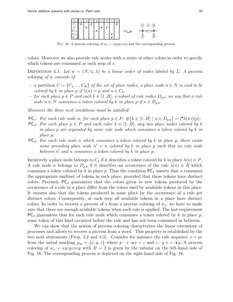
Vector addition systems with states vs. Petri nets 29
ws x y z p z x c y
C1 ✗ ✗ ✗
C2 ✗ ✗ ✗
Dx,1 ✗
Dy,2 ✗
Dz,2 ✗
;
x z
p
x
z
y
c
y
Fig. 16. A process coloring of ws = xyzpzxcy and the corresponding process
colors. Moreover we also provide rule nodes with a series of other colors in order to specifywhich tokens are consumed at each step of s.
Definition 4.1. Let w = (N,6, λ) be a linear order of nodes labeled by Σ. A processcoloring of w consists of
– a partition C = {C1, ..., CB} of the set of place nodes; a place node n ∈ N is said to becolored by k in place p if λ(n) = p and n ∈ Ck.
– for each place p ∈ P and each k ∈ [1..B], a subset of rule nodes Dp,k; we say that a rulenode n ∈ N consumes a token colored by k in place p if n ∈ Dp,k.
Moreover the three next conditions must be satisfied:
PC1: For each rule node n, for each place p ∈ P : #{k ∈ [1..B] | n ∈ Dp,k} = (•λ(n))(p);PC2: For each place p ∈ P and each color k ∈ [1..B], any two place nodes colored by k
in place p are separated by some rule node which consumes a token colored by k inplace p;
PC3: For each rule node n which consumes a token colored by k in place p, there existssome preceding place node n′ < n colored by k in place p such that no rule nodebetween n′ and n consumes a token colored by k in place p.
Intuitively a place node belongs to Ck if it describes a token colored by k in place λ(n) ∈ P .A rule node n belongs to Dp,k if it describes an occurrence of the rule λ(n) ∈ R whichconsumes a token colored by k in place p. Thus the condition PC1 asserts that n consumesthe appropriate multiset of tokens in each place, provided that these tokens have distinctcolors. Precisely PC2 guarantees that the colors given to new tokens produced by theoccurrence of a rule in a place differ from the colors used by available tokens in this place.It ensures also that the tokens produced in some place by the occurrence of a rule getdistinct colors. Consequently, at each step all available tokens in a place have distinctcolors. In order to recover a process of s from a process coloring of ws, we have to makesure that there are enough available tokens when each rule is applied. The last requirementPC3 guarantees that for each rule node which consumes a token colored by k in place p,some token of this kind occurred before the rule and has not been consumed in between.
We can show that the notion of process coloring characterizes the linear extensions ofprocesses and allows to recover a process from a word. This property is established by thetwo next statements (Prop. 4.2 and 4.3). Consider for instance the rule sequence s = pcfrom the initial marking µin = {x, y, z} where p : x ➝ x + z and c : y + z ➝ y. A processcoloring of ws = xyzpzxcy with B = 2 is given by the tabular on the left-hand side ofFig. 16. The corresponding process is depicted on the right-hand side of Fig. 16.
30 Vector addition systems with states vs. Petri nets
Proposition 4.2. Let ws = (N,6, λ) be a linear order of nodes labeled by Σ which cor-responds to the representative word of a rule sequence s ∈ R⋆. Let C = (Ck)k∈[1..B] andD = (Dp,k)p∈P,k∈[1..B] be a process coloring of ws. Let ·≺ be the binary relation over N suchthat x ·≺ y if
– either x is a rule node and y is a following place node with no rule node in between– or y is a rule node and x is a preceding place node colored by k in place p such that y
consumes a token colored with k in place p and no rule node between x and y consumesa token colored with k in place p.
Let 4 be the reflexive and transitive closure of ·≺ . Then the labeled partial order (N,4, λ)is a process of s firable from µin, denoted by KC,D(s). Moreover s is B-bounded.
Proof. We proceed by induction over the length of s. The base case where |s| = 0 istrivial because ·≺ is empty and µin(p) 6 B for each p ∈ P . Induction step. Let s = r1...rm
be a rule sequence of length m > 1 and ws = (N,6, λ) be its representative word. Let(C,D) be a process coloring of ws. We consider the subsequence s′ = r1...rm−1 and itsrepresentative word ws′ = (N ′,6, λ) with N ′ ( N . It is easy to check that the restrictionof the process coloring (C,D) to the nodes from N ′ is a process coloring of ws′. Let ·≺ s′ bethe corresponding binary relation over N ′ and 4s′ be the corresponding partial order. Byinduction hypothesis, (N ′,4s′, λ) is a process K′ of s′ and s′ is a rule sequence firable fromµin and B-bounded. Note that the binary relation ·≺ is acyclic. Moreover the restrictionof (N,4, λ) to nodes of N ′ is precisely the process K′ = (N ′,4s′ , λ) of s′. We need to checkthat adding the nodes from N \N ′ to K′ according to ·≺ yields a process of s. To do so,we check the three next properties:
1. For each place p ∈ P , the rule node n◦ ∈ N \ N ′ corresponding to rk covers at most•rk(p) place nodes labeled by p, i.e. #{n ∈ N ′ | n ·≺ n◦ ∧ λ(n) = p} 6 •rk(p). Thisfollows from PC1 and PC2.
2. For each place p ∈ P , the rule node n◦ ∈ N \ N ′ corresponding to rk covers at least•rk(p) place nodes labeled by p, i.e. #{n ∈ N ′ | n ·≺ n◦ ∧ λ(n) = p} > •rk(p). Thisfollows from PC1 and PC3.
3. The conditions do not branch, i.e. for each place node n ∈ N , if n ·≺ n1 and n ·≺ n2 thenn1 = n2. This is ensured by the definition of ·≺ itself.
It follows that the labeled partial order K = (N,4, λ) is a process of s. Thus s is firablefrom µin. Finally for each place p and each color k, PC2 guarantees that at most one placenode colored by k in place p is not covered by a rule node. Therefore the marking µ reachedby the process K satisfies µ(p) 6 B for all p ∈ P . Thus s is B-bounded.
Thus each process coloring of ws yields a process from [[s]]µin. Consequently s is firable
from µin as soon as it admits a process coloring. With no surprise s has to be B-bounded,too. Conversely the next result asserts that each process of any rule sequence s firable fromµin can be obtained by some process coloring of ws, provided that s is B-bounded.
Proposition 4.3. Let s = r1...rm be a B-bounded rule sequence firable from µin and Kbe a process of s. Then there exists a process coloring (C,D) of the representative word ws
such that KC,D(s) is isomorphic to K.
Vector addition systems with states vs. Petri nets 31
Proof. We proceed by induction over the length of s. The base case where |s| = 0 is trivialbecause µin is B-bounded. Induction step. Let K = (B∪E,F ∗, λ) be a process of s = r1...rm
of length m > 1 with set of conditions C and set of events E. We consider the subsequences′ = r1...rm−1 and the prefix K′ = (B′ ∪ E ′, F ∗, λ) of K in which the event e◦ ∈ Ecorresponding to the last occurrence of rm and the subsequent conditions are removed.Clearly K′ is a process of s′. By induction hypothesis, there exists a process coloring(C ′, D′) of ws′ such that KC′,D′(s′) = (N ′,4C′,D′, λ) is isomorphic to K′ = (B′ ∪ E ′, F, λ).We let σ : B′ ∪E ′ → N ′ denote an isomorphism from K′ to KC′,D′(s′), i.e. a bijection suchthat
– x1F∗x2 iff σ(x1) 4C′,D′ σ(x2) for all x1, x2 ∈ B′ ∪E ′ and
– λ(σ(x)) = λ(x) for all x ∈ B′ ∪ E ′.
We extend the bijection σ : B′ ∪ E ′ → N ′ to a bijection σ : B ∪ E → N such that
– σ(e◦) is the rule node from N \N ′, and– each condition c from B\B′ maps to a place node σ(c) ∈ N\N ′ such that λ(σ(c)) = λ(c).
We extend also the process coloring (C ′, D′) to a process coloring (C,D) of ws in two steps:
1. For all places p ∈ P and for all colors k ∈ [1..B], the rule node σ(e◦) belongs to Dp,k ifthe event e◦ covers a condition c such that the corresponding node σ(c) is labeled by pand colored by k, i.e. λ(c) = p and σ(c) ∈ C ′
k.2. The colors of the additionnal place nodes from N \N ′ are chosen arbitrarily such that
all maximal conditions of K labeled by the same place p have distinct colors. This ispossible because the marking reached by s is B-bounded.
We can check that the resulting coloring (C,D) is a process coloring.
PC1: Let p ∈ P and n◦ = σ(e◦). Since K is a process, #{k ∈ [1..B] | n◦ ∈ Dp,k} 6
(•λ(n◦))(p). We can check that all conditions labeled by p and covered by the evente◦ have distinct colors, because of PC2. Thus #{k ∈ [1..B] | n◦ ∈ Dp,k} = (•λ(n◦))(p).
PC2: The required property holds for any two place nodes from ws′ because (C ′, D′) is aprocess coloring. It holds also by construction for any two place nodes from N \N ′. Itholds also obviously if one place node belongs to N ′ and the other to N \N ′ becausethe rule node n◦ occurs in between.
PC3: The required property holds for each rule node n ∈ N ′. Let p ∈ P and k ∈ [1..B] besuch that n◦ ∈ Dp,k. By definition of Dp,k the event e◦ covers a condition c such thatthe corresponding node n = σ(c) is labeled by p and colored by k. Moreover there isno rule node n′ between n and n◦ with n′ ∈ Dp,k. Otherwise the condition c wouldbe also covered by some event in K′, hence c would be a branching condition in K.
Recall that σ maps each condition from B \B′ to a place node from N \N ′ with the samelabel. All these conditions cover e◦ and all these place nodes cover σ(e◦). To conclude, weneed to check that for each place node n ∈ N ′, we have n ·≺ C,Dn
◦ in KC,D(s) if and onlyif σ−1(n)Fe◦ in K.
32 Vector addition systems with states vs. Petri nets
Assume first that n ·≺ C,Dn◦. Then there exists a place p ∈ P and a color k ∈ [1..B]
such that λ(n) = p, n ∈ Ck, and n◦ ∈ Dp,k. Further there exists some condition c in theprocess K such that cFe◦, λ(c) = p and σ(c) ∈ Ck. Then σ(c) = n because of PC2. Henceσ−1(n)Fe◦ in K.
Conversely, assume now that σ−1(n)Fe◦ in K. Let p = λ(n) and k be the color suchthat n ∈ Ck. We have n◦ ∈ Dp,k according to the definition of Dp,k. No event in K′ coversσ−1(n) so there exists no rule node in ws′ after n which is colored by Dp,k. It follows thatn ·≺ C,Dn
◦.Thus the notion of process coloring characterizes the processes of any B-bounded rulesequence firable from µin.
Following the easy part of Buchi Theorem, we can design an MSO formula φS whichdefines the words w = (N,6, λ) over Σ which are representative words of a computationsequence of S. We can also design a formula φpc(C,D) with B × (|P | + 1) second-orderfree variables C = (Ck)k∈[1..B] and D = (Dk,p)k∈[1..B],p∈P which characterizes the notion ofa process coloring for a word w = (N,6, λ) over Σ. Moreover, by means of Prop. 4.2,we can build a formula φ4(x, y, C,D) with two first-order free variables x and y andB×(|P |+1) second-order free variables such that for any interpretation of C = (Ck)k∈[1..B]
and D = (Dk,p)k∈[1..B],p∈P and any interpretation of x and y, φ4(x, y, C,D) is satisfied ifand only if we have x 4 y in the process corresponding to the process coloring given bythe interpretation.
Let ψ be an MSO sentence for labeled partial orders over Σ. We consider the followingformula ψS for words over Σ:
ψS = φS ∧ ∃C, ∃D, (φpc(C,D) ∧ ¬ψ′(C,D))
where the formula ψ′(C,D) is obtained from ψ by replacing each occurrence of x 4 y byφ4(x, y, C,D). Thus a word satisfies ψS if (and only if) it is a representative word of acomputation sequence s of S for which there exists a process coloring which describes aprocess satisfying ¬ψ. In this way we get the main result of this section.
Theorem 4.4. Let S be a bounded PNS and ψ be an MSO sentence over causal nets. Allprocesses of S satisfy ψ if and only if the word sentence ψS is not satisfiable.
Thus the model-checking problem for a bounded PNS against an MSO-sentence is decid-able. In practice, the unsatisfiability of ψS is reduced to the emptiness problem of a finiteautomaton. It is of course more efficient not to include the sentence φS and to compare theresulting automaton with the automaton that recognizes the representative words of com-putation sequences of S. Noteworthy we could provide the PNS S with a subset of acceptingstates and check alternatively that all processes derived from an accepting computationsequence satisfy ψ.
4.3 Comparisons to related works
This result subsumes previous works in several extents. A cMSG is said to be safe if allpaths from the initial state to some fixed state lead to the same marking. Consequently,
Vector addition systems with states vs. Petri nets 33
any safe PNS is bounded. This constraint is interesting because checking whether a PNSis bounded and computing a bound is hard and requires exponential space [11]. Yet thetechnique presented in this section allows us to check effectively MSO properties of theprocesses derived from a bounded (non-safe) cMSG or more generally a bounded PNS.Since MSO behaviours can be characterized by some MSO sentence, this result extendsthe main result from [26] which asserts that the model-checking problem for safe cMSGs isdecidable (see also [13, Cor 6.1]). As opposed to [13, 26], we do not assume FIFO behavioursand consequently we cannot make use of the notion of representative linearizations. Thefact is that, as already mentionned, a computation sequence can correspond to several non-isomorphic processes depending on the order identical particles are consumed. Thereforewe need the notion of process coloring (Def. 4.1) to recover a process from a word. Thisis the main difference with the setting of MSCs because these are completely specifiedby any of their linearizations. Still, the FIFO restriction can be formalized in MSO logicand our technique applies also in this special case. Second Petri nets and VASSs abstractaway from the notions of sites and channels in the setting of MSCs: A place can describethe local state of a site, a communication channel, a shared-variable, etc. In particularour approach applies to any bounded Petri net. To the best of our knowledge, the modelchecking problem of bounded Petri nets against MSO formulae under the process semanticshas not been investigated so far in the literature. We show with an example below thatthe process semantics of Petri nets can be used to model and check systems with specificbehavioural constraints, such as FIFO channels, causal communication, or private keys, assoon as these restrictions can be formalized by an MSO sentence. Note finally that it maybe possible to encode a bounded Petri net with a safe cMSGs. However this requires torepresents each reachable marking by a distinct control state so the size of the resultingcMSG would be exponential in the size of the Petri net even for 1-safe Petri nets.
5 Conclusion
We introduce a natural partial order semantics for vector addition systems with states(and Petri nets with states) which extends the non-branching process semantics of Petrinets and follows the asynchronous approach of message sequence charts. We show howbasic problems about the set of markings reached along concurrent executions, such asboundedness, covering and reachability, can be solved similarly to the analogous problemsfor Petri nets. We show also how to check effectively any MSO property of these partialorders provided that the system is bounded. This result generalizes results known formessage sequence graphs and is new, even in the restricted case of Petri nets.
However vector addition systems with states are not always as easy as Petri nets tohandle. We have observed that vector addition systems with states are more expressive than(pure) Petri nets under this process semantics. Moreover the synthesis problem of Petri netsfrom prefix-bounded vector addition systems with states turns out to be undecidable. Asa consequence we have illustrated the gap between Petri nets and vector addition systemswith states as follows: It is undecidable whether two prefix-bounded vector addition systemswith states are semantically equivalent, contrary to Petri nets.

34 Vector addition systems with states vs. Petri nets
Introduced as a formal model for the semantics of elementary Petri nets, Mazurkie-wicz traces [27] are particular labeled partial orders that benefit from a rich and stillgrowing theory [7]. In particular we have made use of the undecidability of the universalityproblem for rational trace languages to establish all undecidability results presented in thispaper. We have shown that Mazurkiewicz traces can be described as the processes of veryparticular prefix-bounded systems. However Mazurkiewicz trace theory enjoys several nicepositive results for particular rational languages. Most of these results have been alreadyadapted to the setting of message sequence charts (see in particular [19]). Thus, this studyleads us to investigate an extension of Mazurkiewicz trace theory to the whole setting ofprefix-bounded Petri nets with states. Moreover some classes of Petri nets with states forwhich realizability and prefix-realizability become decidable might arise from this study.
References
1. R. Alur, K. Etessami, and M. Yannakakis. Inference of message sequence charts. IEEE Transactions onSoftware Engineering, 29(7):623–633, 2003.
2. R. Alur and M. Yannakakis. Model checking of message sequence charts. In Jos C. M. Baeten and SjoukeMauw, editors, CONCUR, volume 1664 of Lecture Notes in Computer Science, pages 114–129. Springer, 1999.
3. H. Ben-Abdallah and S. Leue. Syntactic detection of process divergence and non-local choice in messagesequence charts. In Ed Brinksma, editor, TACAS, volume 1217 of Lecture Notes in Computer Science, pages259–274. Springer, 1997.
4. E. Best and R. R. Devillers. Sequential and concurrent behaviour in Petri net theory. Theoretical ComputerScience, 55(1):87–136, 1987.
5. J.R. Buchi. Weak second-order arithmetic and finite automata. Z. Math. Logik Grundlagen Math., 6:66–92,1960.
6. Ph. Darondeau. Unbounded Petri Net Synthesis. In Jorg Desel, Wolfgang Reisig, and Grzegorz Rozenberg,editors, Lectures on Concurrency and Petri Nets, volume 3098 of Lecture Notes in Computer Science, pages413–438. Springer, 2003.
7. V. Diekert and G. Rozenberg. The Book of Traces. World Scientific Publ. Co., 1995.
8. M. Droste, P. Gastin, and D. Kuske. Asynchronous cellular automata for pomsets. Theoretical ComputerScience, 247(1-2):1–38, 2000.
9. A. Ehrenfeucht and G. Rozenberg. Partial (set) 2-structures. Part II: State spaces of concurrent systems. ActaInformatica, 27(4):343–368, 1989.
10. J. Engelfriet. Branching processes of Petri nets. Acta Informatica, 28:575–591, 1991.
11. J. Esparza and M. Nielsen. Decidability issues for Petri nets - a survey. Bulletin of the EATCS, 52:244–262,1994.
12. J. Esparza, S. Romer, and W. Vogler. An improvement of McMillan’s unfolding algorithm. Formal Methodsin System Design, 20:285–310, 2002.
13. B. Genest, D. Kuske, and A. Muscholl. A Kleene theorem and model checking algorithms for existentiallybounded communicating automata. Inf. Comput., 204(6):920–956, 2006.
14. H.J. Genrich and E. Stankiewicz-Wiechno. A dictionary of some basic notions of net theory. In Wilfried Brauer,editor, Advanced Course: Net Theory and Applications, volume 84 of Lecture Notes in Computer Science, pages519–531. Springer, 1975.
15. R. J. van Glabbeek, U. Goltz, and J.-W. Schicke. On causal semantics of Petri nets. In Joost-Pieter Katoen andBarbara Konig, editors, CONCUR, volume 6901 of Lecture Notes in Computer Science, pages 43–59. Springer,2011.
16. U. Goltz and W. Reisig. The non-sequential behavior of Petri nets. Information and Control, 57(2/3):125–147,1983.
17. J. Grabowski. On partial languages. Fundamenta Informaticae, 4(2):427–498, 1981.
18. E. L. Gunter, A. Muscholl, and D. Peled. Compositional message sequence charts. In Tiziana Margaria andWang Yi, editors, TACAS, volume 2031 of Lecture Notes in Computer Science, pages 496–511. Springer, 2001.

Vector addition systems with states vs. Petri nets 35
19. J. G. Henriksen, M. Mukund, K. Narayan Kumar, M. A. Sohoni, and P. S. Thiagarajan. A theory of regularMSC languages. Information and Computation, 202(1):1–38, 2005.
20. P. W. Hoogers, H. C. M. Kleijn, and P. S. Thiagarajan. A trace semantics for Petri nets. Information andComputation, 117(1):98–114, 1995.
21. J.E. Hopcroft and J-J. Pansiot. On the reachability problem for 5-dimensional vector addition systems. The-oretical Computer Science, 8:135–159, 1979.
22. R.M. Karp and R.E. Miller. Parallel program schemata. Journal of Computer and System Sciences, 3(2):147–195, 1969.
23. A. Kiehn. On the interrelation between synchronized and non-synchronized behaviour of Petri nets. Journal ofInformation Processing and Cybernetics / Elektronische Informationsverarbeitung und Kybernetik, 24(1/2):3–18, 1988.
24. S. Leue, R. Mayr, and W. Wei. A scalable incomplete test for the boundedness of UML RT models. In KurtJensen and Andreas Podelski, editors, TACAS, volume 2988 of Lecture Notes in Computer Science, pages327–341. Springer, 2004.
25. P. Madhusudan. Reasoning about sequential and branching behaviours of message sequence graphs. In Fer-nando Orejas, Paul G. Spirakis, and Jan van Leeuwen, editors, ICALP, volume 2076 of Lecture Notes inComputer Science, pages 809–820. Springer, 2001.
26. P. Madhusudan and B. Meenakshi. Beyond message sequence graphs. In Ramesh Hariharan, MadhavanMukund, and V. Vinay, editors, FSTTCS, volume 2245 of LNCS, pages 256–267. Springer, 2001.
27. A. Mazurkiewicz. Concurrent program schemes and their interpretation. Technical report, DAIMI ReportPB-78, Aarhus University, 1977.
28. M. Mukund. Petri nets and step transition systems. International Journal of Foundations of Computer Science,3(4):443–478, 1992.
29. M. Nielsen, G. Plotkin, and G. Winskel. Petri nets, event structures and domains, part I. Theoretical ComputerScience, 13:85–108, 1981.
30. J. L. Peterson. Petri Net Theory and the Modeling of Systems. Englewood Cliffs, New Jersey: Prentice Hall,Inc., 1981.
31. C. A. Petri. Non-Sequential Processes: Translation of a Lecture given at the IMMD Jubilee Colloquium on‘Parallelism in Computer Science’, Universitat Erlangen-Nurnberg. St. Augustin: Gesellschaft fur Mathematikund Datenverarbeitung Bonn, Interner Bericht ISF-77–5, 1977.
32. C. Rackoff. The covering and boundedness problems for vector addition systems. Theoretical Computer Science,6:223–231, 1978.
33. W. Reisig. Petri Nets, An Introduction. EATCS Monographs, vol. 4. Springer, 1985.34. C. Reutenauer. The Mathematics of Petri Nets. New York, USA: Prentice-Hall, 1990.35. J. Sakarovitch. The ”last” decision problem for rational trace languages. In Imre Simon, editor, LATIN,
volume 583 of Lecture Notes in Computer Science, pages 460–473. Springer, 1992.36. J. Sakarovitch. Elements of Automata Theory. Cambridge University Press, 2009.37. W. Vogler. Modular Construction and Partial Order Semantics of Petri Nets, volume 625 of Lecture Notes in
Computer Science. Springer, 1992.38. W. Zielonka. Notes on finite asynchronous automata. R.A.I.R.O. - Informatique Theorique et Applications,
21:99–135, 1987.