Embed Size (px)
Citation preview

VC.07
Change of Variables to Compute Double Integrals

Example 1: A Familiar Double Integral
Use a double integral to calculate the area of a circle of radius 4 centered
at the origin:
2 2The region R is given by x y 16: R
1dA
2
2
4 16 x
4 16 x
1dA
Now dA means "a small change in area" in
xy-coordinates. We can measure a small change
in area with a little rectangle.2
2
4 16 x
4 16 x
1dy dx
So dA = dy dx:
dA
dx
dy

Example 1: A Familiar Double Integral
This integral is actually pretty complicated to evaluate:2
2
4 16 x
4 16 x
1dy dx
4
2
4
2 16 x dx
4
2 1
4
x16 x 16sin
4
16
What a mess! There must be a better way to
use integration to do this...
What coordinate system would you prefer to
use to when dealing with a region like R?
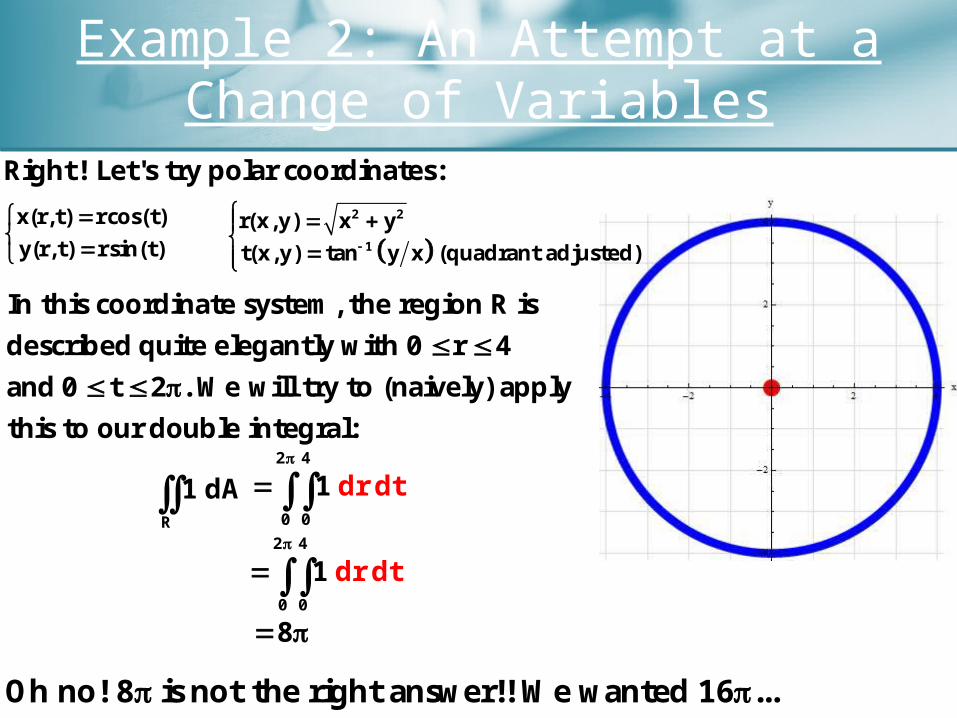
Example 2: An Attempt at a Change of Variables
Right! Let's try polar coordinates:
In this coordinate system, the region R is
describedquite elegantly with 0 r 4
and0 t 2 . We will try to (naively) apply
this to our double integral:
2 4
0 0
d t1 r d
R
1dA2 4
0 0
d t1 r d
x(r,t) rcos(t)
y(r,t) rsin(t)
2 2
1
r(x,y) x y
t(x,y) tan y x (quadrant adjusted)
8
Oh no! 8 isnot the right answer!! We wanted 16 ...

Detour: Working Out the Change of Variables the Right Way
Our misconception was that dA . Our dA refers to a small change
in xy-area, not rt-area. We need to delve a bit deeper to sort this
dr dt
out:
2
2
4 16 x 2 4
4 0 016 x
For 1dy dx our region was a circle, while 1 looks more
likethe integral you'd take for a rectangle:
dr dt
x(r,t) rcos(t)
y(r,t) rsin(t)
2 2
1
r(x,y) x y
t(x,y) tan y x

Detour: Working Out the Change of Variables the Right Way
Let's analyze the transformation T(r,t) rcost,rsint piece bypiece
and verify that the picture shown below makes sense:
x(4, ) 4cos
y(4, ) 4sin
For the blue line,
r 4,0 t 2 :
x(r,0) r
y(r,0) 0
For the green line,
t 0,0 r 4:
x(r,2 ) r
y(r,2 ) 0
For the orange line,
t 2 ,0 r 4:
Let's map a few points
just for practice:
This whole process can be called a mapping,a transformation,
a change of variables, or a change of coordinates.
x(0,t) 0
y(0,t) 0
For the red line,
r 0,0 t 2 :
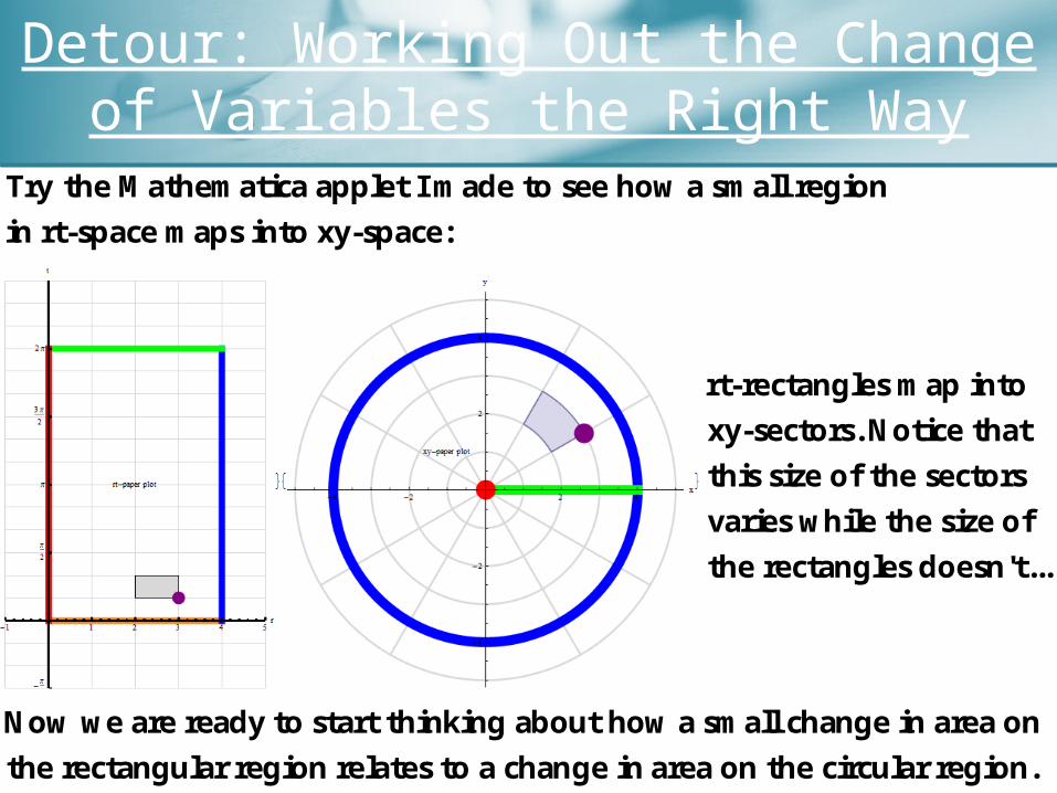
Detour: Working Out the Change of Variables the Right Way
Try the Mathematica applet I made to see how a small region
in rt-space maps into xy-space:
Now we are ready to start thinking about how a small change in area on
the rectangular region relates to a change inarea on the circular region.
rt-rectangles map into
xy-sectors.Notice that
this size of the sectors
varies while the size of
the rectanglesdoesn't...

Detour: Working Out the Change of Variables the Right Way
(r,t)
Now imagine a very small rectangle in the rt-plane:
(r r,t)
(r r,t t) (r,t t)
T(r,t)T(r r,t)
T(r r,t t)
T(r,t t)
That is, consider the limit as A, r,and t tendto 0: T(r r,t) T(r,t)
T(r r,t) T(r,t) rr
T(r,t t) T(r,t)T(r,t t) T(r,t) t
t
These approximations using partial derivatives let us approximate
our sector using a parallelogram:
Tr
r
Tt
t

Detour: Working Out the Change of Variables the Right Way
(r,t)
Now imagine a very small rectangle in the rt-plane:
(r r,t)
(r r,t t) (r,t t)
T(r,t)
T(r r,t)
T(r r,t t)
T(r,t t)
Tr
r
Tt
t
Theorem: The area of the parallelogram formed by two
vectorsV and W equals V W .
Tr
TtA
tr
Tt
Ttr
r
(We can take a scalar out of
either vector in a cross product)
1 2
1 2
i
T Tr
r r
j
t
T T
t t
k
0
0
2
1 2
1
tT T
t
T T
r r r
t
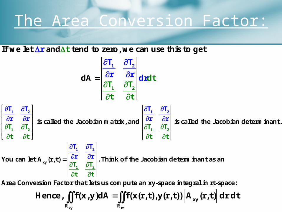
The Area Conversion Factor:
1 2
1 2
If we let and tend to zero, we can usr
T T
r
e tt
dtT T
t
r d
his t
t
et
d r
o g
A
xy rt
xyR R
Hence, f(x,y)dA f(x(r,t),y(r,t)) A (r,t) dr dt
1 2
1 1
1 2
2 2
is called the Jacobian matrix, and is called the Jacobian determi
T T T T
T T T T
t t t t
r r n .r ar nt
x1 2
1 2
yYou can let A (r,t) . Think of the Jacobian determinant as an
Area Conversion Factor that lets us compute an xy-space integ
T
r
T
r r
al in rt-spat
:
T
tc
T
e

The Area Conversion Factor:
xy rt
xyR R
f(x,y)dA f(x(r,t),y(r,t)) A (r,t) dr dt
1 2
xy
1
1 2
2
Let T(r,t) be a transformation from rt-space to xy-space.
That is, T(r,t) T (r,t),T (r,t) (x(r,t),y(r,t)).
ThenA
T T
r(r,tT
t t
) .T
r
xyNote: Since we derived A (r,t) as the magnitude of a cross product,we need
it to be positive. This is why we put absolute value bars into the formula above.
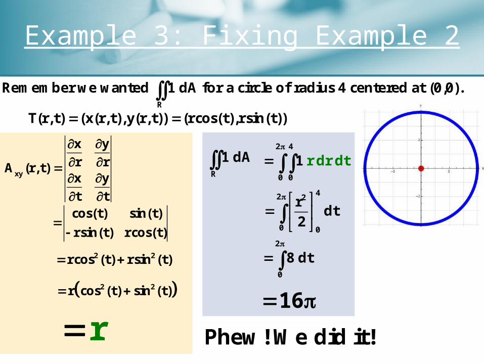
Example 3: Fixing Example 2
R
Remember we wanted 1dA for a circle of radius 4 centered at (0,0).
2 4
0 0
r d t1 r d
R
1dA42 2
0 0
rdt
2
2
0
8dt
T(r,t) (x(r,t),y(r,t)) (rcos(t),rsin(t))
xy
yxr rA (r,t)
yxt t
cos(t) sin(t)
rsin(t) rcos(t)
2 2rcos (t) rsin (t)
r 2 2r cos (t) sin (t)
16
Phew!We did it!
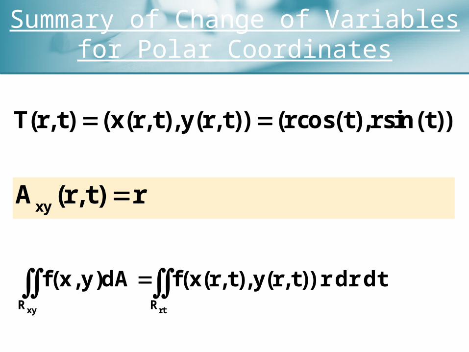
Summary of Change of Variables for Polar Coordinates
T(r,t) (x(r,t),y(r,t)) (rcos(t),rsin(t))
xyA (r,t) r
xy rtR R
f(x,y)dA f(x(r,t),y(r,t))r dr dt

• By now you probably already asked yourself why this change of variables is useful. This was just a circle of course! We could have used A = πr2 or the Gauss-Green formula.
• Hence, we should look at an example where a double integral in xy-coordinate space would be horribly messy, the boundary region is hard to parameterize for Gauss-Green, and we can’t just plug into a familiar area formula…
Example 4: More With Polar Coordinates

This would have been HORRIBLE in rectangular coordinates.
Butusing polar coordinates, and this
is the rt-rectangle w
x rcos(t) y rsin(t)
ith0 t and2 r 5:
Example 4: More With Polar Coordinates
2 2
R
2 2 2 2
Compute x y dA for the region satisfying the following inequalities:
x y 25,x y 4,y 0
5
2 2
0 2
rcos(t) rsin(t) r dr dt
2 2
R
x y dA5
3
0 2
r dr dt
0
609dt
4
6094
Substitute x rcos(t)and y rsin(t)

Analogy Time:
xy uv
xyR R
f(x,y)dA f(x(u,v),y(u,v)) A (u,v) dudv This should be reminiscent of change of variables for single-variable calculus:
This whole change of variables thing isn't just for polar coordinates.
We can change from xy-space to any uv-coordinate space we want:
x(b) b
x(a) a
f(x)dx f(x(u)) x'(u)du
xySo you can think of the Jacobian Determinant, A (u,v) , as a
higher-dimensional analogue of x'(u) in our old friend, u-substitution.
Let's try one in a single variable:

Example 5: Change of Variables for Single Variable Calculus
x(b) b
x(a) a
f(x)dx f(x(u)) x'(u)du 6
2
e
e
ln(x)Compute dx.
x
u
u
ln(x)f(x)
xx(u) e
x'(u) e
6
2
f(x(u)) x'(u)du6
u u
2
f(e )e du6
uu
2
ue du
e
62
2
u2
16
It works! This is the same as
your more familiar method:
u ln(x)
1du dx
x
6
2
udu 16

• As I said, a change of variables isn’t just good for polar coordinates. We’ll try a few regions tomorrow that require a different change of variables with a different Jacobian determinant (area conversion factor).
Next Up:

xy
Let's let and for 0 v 2 and
0 u 1. These are NOT polar coordinates, so we nee
x 2ucos(v) y us
d
to com
i
p
n
ute A (u,v) :
(v)
Example 6: Beyond Polar Coordinates
2
2 2
R
xCompute y dA for the region given by the ellipse y 1.
2
xy
yxu uA (u,v)
yxv v
2cos(v) sin(v)
2usin(v) ucos(v)
2 22ucos (v) 2usin (v)
2u 2 22u cos (v) sin (v)

Example 6: Beyond Polar Coordinates
2
2 2
R
xCompute y dA for the region given by the ellipse y 1.
2
22
21
0 0
2ududvu sin (v)
2
R
y dA2 1
3 2
0 0
2 u sin (v)dudv
g
u 12 42
0 u 0
u2 sin (v) dv
4
g
Substitute x 2ucos(v)
and y usin(v)
22
0
1sin (v)dv
2
2

Example 7: Mathematica-Aided Change of Variables (Parallelogram Region)
y
R
UseMathematica to compute e dA for R given by the parallelogram:These lines are given by ,
1 13 1y x y x 6
4 4 4
,
,and .
y x 1 y x 4
1 yWe xcan rewrite them as ,
1 13 1x y x y 6
,
,and .
x
4 4
4 y
4
But to computeour integral, we need the map from uv-space to xy-space...
v(x,yThat is, we have and ,but we need u(x,y) x(u,v) y(ua d) n ,v).
Solve[LetMathematica { [ , ], [ , ]},{ , }]do the work: u u x y v v x y x y
1T
13v x y v 6
4henwe can let and for andy 4 !u u 1
4x
and1
y4
x (u 4v) )(u5 5
v

Example 7: Mathematica-Aided Change of Variables (Parallelogram Region)
y
R
UseMathematica to compute e dA for R given by the parallelogram:
and1
y4
x (u 4v) )(u5 5
v
xy
yxu uA (u,v)
yxv v
4 15 54 45 5
45
So we use45

Example 7: Mathematica-Aided Change of Variables (Parallelogram Region)
y
R
UseMathematica to compute e dA for R given by the parallelogram:
xy
1y (
4A (u,v) , , ,
5
for an
u 4v)5
13v 6d :
4x (u
4
v)5
4 u 1
y
R
e dA6 1
(u 4v)/5
13/ 4 4
4dudv
5e
417.1 (fromMathematica)