VC-Dimension and Rademacher Averages:From Statistical Learning Theory to Sampling Algorithms

Matteo Riondato1,2 Eli Upfal1

1

Department of Computer Science – Brown University

2

Now at Two Sigma Investments

ECML PKDD’15 – Porto, September 11, 2015

Why this tutorial?

Over the years, we became convinced of the mathematical elegance of statisticallearning theory. Experimental results then showed us its practical power.

We believe VC-dimension and Rademacher Averages are under-utilized in research andunder-taught in classes, often relegated to small-font paragraphs in ML textbooks (thisis slowly changing).

We feel that developing data mining algorithms using techniques considered to be onlyrelevant for the theory of machine learning can help bringing the ML and the DMcommunities together...like ECML PKDD!

Logistics

You can find these slides at http://bit.ly/1JZEfF5

Tutorial mini-website: http://bigdata.cs.brown.edu/vctutorial/

Slides, bibliography, ...

Please interrupt me and ask questions at any time

Live tweet hashtag: #vctutorial

Two Views of Data 

•  The DB approach: The dataset is the whole truth (and nothing but the truth) –  Example:  Abnormality detec9on ‐ Given a sequence of NASDAQ transac9ons, find suspicious transac9ons 

•  The scien9fic approach: The dataset is a sample of a larger process or system 

– Generaliza9on: Valid observa9ons on a sample must hold on other samples from the system 

Data Analysis Through Sampling 

•  Sampling is a powerful technique –analyzing a sample, instead of the whole data set, saves computa9onal 9me and space 

•  Analyzing a sample gives an approxima9on of the “true” result (but the whole data set may also be a sample) 

The main ques9on: How good 

is an approxima9on obtained 

from analyzing a sample (of a 

given size)? 

How Good is the Approxima9on? 

•  We “know” that increasing the sample size improves the approxima9on results 

•  Can we quan9fy this rela9on? •  We want a statement of the form:  

 “When analyzing a random sample of size n, with probability 1‐ δ, the results are within an ε factor (addi9ve of mul9plica9ve) of the true results.”  

We need more informa9on… 

The Fundamental Tradeoff: 

  

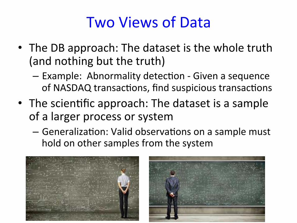
–  Sample size 

– Accuracy of the results –  Complexity of the analysis task 

 

VC‐Dimension and Rademacher Averages are two measures for the complexity of the analysis task 

 

Using these measures we can obtained almost 9ght rela9ons between the three quan99es 

Two Major Sampling Tasks 

Detec9on: 

•  Detect internet flows sending more than 5% 

of total packet traffic 

•  Learn a classifica9on rule from a training set  

Es9ma9on: 

•  Es9mate the market share of all internet 

browsers with at least 5% market share 

•  Find the top frequent itemsets in a dataset 

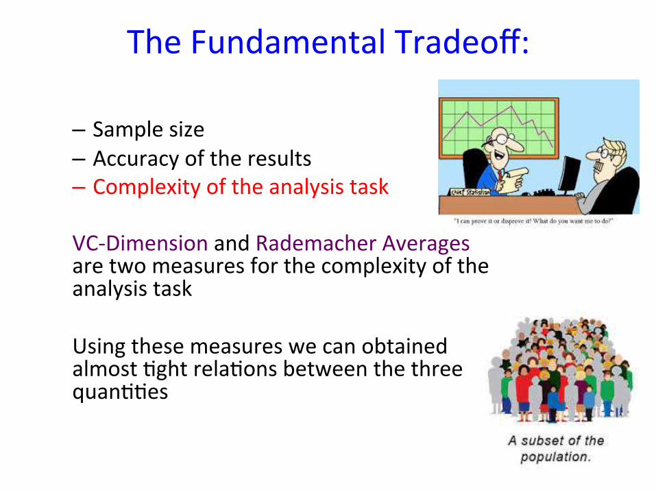
Basic Sampling ResultsConsider uniform sampling S from a set U. Let R ™ U, such that |R| Ø ‘|U|.

Claim (Detection)If S is a uniform random sample of U with size Ø 1

‘ ln 1

” then

Pr(S fl R = ÿ) Æ (1 ≠ ‘) 1

‘ ln

1

” Æ ”

Claim (Estimation – Cherno� bound)If S is a uniform random sample of U with size Ø 3

‘3

ln 2

” then

Pr3----

|S fl R||S| ≠ |R|

|U|

---- Æ ‘|R||U|

4Ø 1 ≠ ”

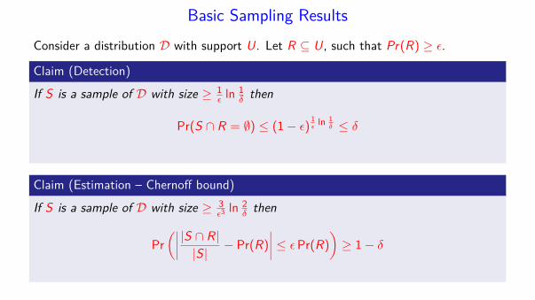
Basic Sampling ResultsConsider a distribution D with support U. Let R ™ U, such that Pr(R) Ø ‘.

Claim (Detection)If S is a sample of D with size Ø 1

‘ ln 1

” then

Pr(S fl R = ÿ) Æ (1 ≠ ‘) 1

‘ ln

1

” Æ ”

Claim (Estimation – Cherno� bound)If S is a sample of D with size Ø 3

‘3

ln 2

” then

Pr3----

|S fl R||S| ≠ Pr(R)

---- Æ ‘ Pr(R)4

Ø 1 ≠ ”

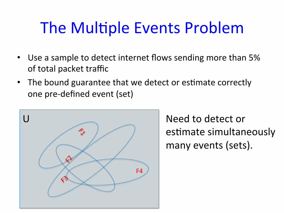
The Mul9ple Events Problem 

•  Use a sample to detect internet flows sending more than 5% 

of total packet traffic 

•  The bound guarantee that we detect or es9mate correctly 

one pre‐defined event (set) 

U  Need to detect or 

es9mate simultaneously 

many events (sets). 

F4 

Uniform convergence

Basic sampling results guarantee that a sample intersects or approximate one givenevent (set), if the sample is not too small

Instead, we want a sample that intersects or approximates simultaneously all events(sets) that are not too small

• More than one event• Not fixed in advance

Classical solution to this problem: Union bound

The union boundConsider uniform sampling S from a set U. Let R

1

, . . . , Rn be subsets of U, such that|Ri | Ø ‘|U|, 1 Æ i Æ n.

Claim (Estimation )If S is a uniform random sample of U with size Ø 3

‘3

ln 2n” then

Pr3

÷i s.t.----|S fl Ri |

|S| ≠ |Ri ||U|

---- > ‘|Ri ||U|

4< ”

The sample size now depends on the number n of sets we are interested inapproximating!

Union bound consider events as if they were disjoint! This is far too loose!

Not practical for many applicationse.g., n is the number of itemsets, or of nodes in a graph!

PAC learning of a binary classifier

Consider:• A probability distribution fi on a domain D• A partition c of D into In and Out classes• A concept class C – a collection of classification rules that includes the true

classification c (realizable case)The learning algorithm gets m training examples (x , c(x)), where x is sampled from fi

Probably Approximately Correct (PAC) Learning:With probability 1 ≠ ”, the algorithm returns a classification rule from C that is

correct (on elements sampled from fi) with probability 1 ≠ Á

Learning a Binary Classifier 

•  Out and In items, and possible classifica9on rules 

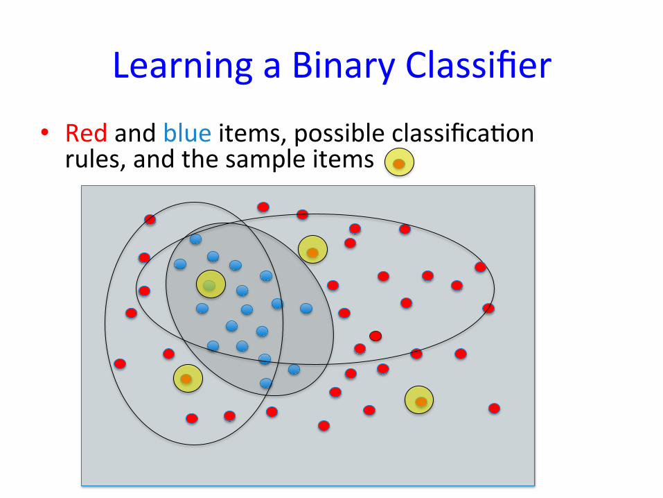
Learning a Binary Classifier 

•  Red and blue items, possible classifica9on rules, and the sample items 

When does the sample identify the correct rule?

• C - concept class - a collection of possible classification rules.• c œ C - the correct rule.• For any h œ C let �(c, h) be the set of items on which the two classifiers di�er:

�(c, h) = {x œ U | h(x) ”= c(x)}

• We need a sample that intersects every set in the family of sets

{�(c, h) | Pr(�(c, h)) Ø ‘}

Definition (‘-net )An ‘-net is a set S ™ U such that for any R ™ U, if Pr(R) Ø ‘ then |R fl S| Ø 1.

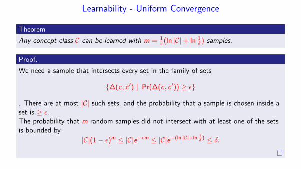
Learnability - Uniform Convergence

TheoremAny concept class C can be learned with m = 1

‘ (ln |C| + ln 1

” ) samples.

Proof.We need a sample that intersects every set in the family of sets

{�(c, c Õ) | Pr(�(c, c Õ)) Ø ‘}

. There are at most |C| such sets, and the probability that a sample is chosen inside aset is Ø ‘.The probability that m random samples did not intersect with at least one of the setsis bounded by

|C|(1 ≠ ‘)m Æ |C|e≠‘m Æ |C|e≠(ln |C|+ln

1

” ) Æ ”.

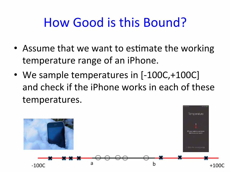
How Good is this Bound? 

•  Assume that we want to es9mate the working 

temperature range of an iPhone. 

•  We sample temperatures in [‐100C,+100C] 

and check if the iPhone works in each of these 

temperatures. 

‐100C  +100C a  b 

Learning an Interval 

•  Our universe U is an interval [A,B] on the line •  The “In” points are in the sub interval [a,b], the “out” points are outside [a,b] 

•  Our concept class is the collec9on of all the intervals [c,d], A ≤ c < d ≤ B 

•  If the learning algorithm returned the interval [x,y] then there were no samples in the sub‐intervals [x,a] and [y,b] 

A  B a  b 

x  y 

Learning an Interval

• A distribution D is defined on universe that is an interval [A, B].• The true classification rule is defined by a sub-interval [a, b] ™ [A, B].• The concept class C is the collection of all intervals,

C = {[c, d ] | [c, d ] ™ [A, B]}

TheoremThere is a learning algorithm that given a sample from D of size m = 2

‘ ln 2

” , withprobability 1 ≠ ”, returns a classification rule (interval) [x , y ] that is correct withprobability 1 ≠ ‘.

Note that the sample size is independent of the size of the concept class |C|, which is(B ≠ A)2 if we assume that x and y must be integers, and infinite otherwise.

Proof.Algorithm: Choose the smallest interval [x , y ] that includes all the ”In” sample points.

• Clearly a Æ x < y Æ b, and the algorithm can only err in classifying ”In” points as”Out” points.

• Fix a < aÕ and bÕ < b such that Pr([a, aÕ]) = ‘/2 and Pr([b, bÕ]) = ‘/2.• If the probability of error when using the classification [x , y ] is Ø ‘ then either

aÕ Æ x or y Æ bÕ or both.• The probability that the sample of size m = 2

‘ ln 2

” did not intersect with one ofthese intervals is bounded by

2(1 ≠ ‘

2)m Æ e≠ ‘m2

+ln 2 Æ ”

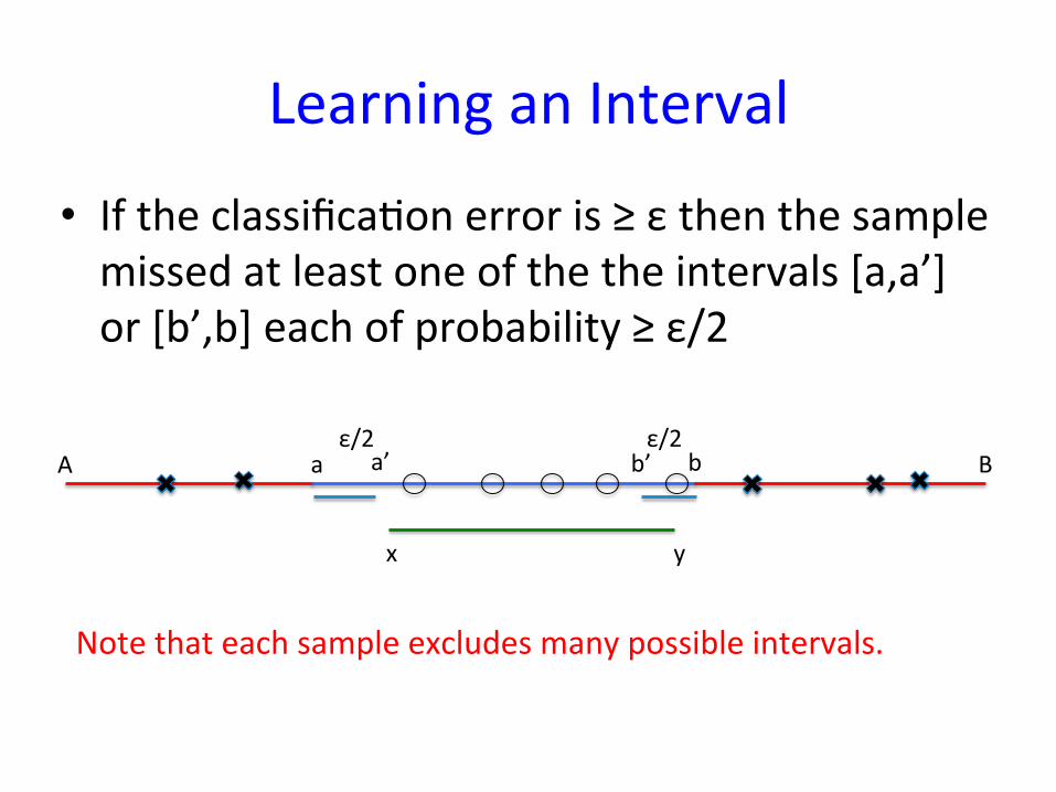
Learning an Interval 

•  If the classifica9on error is ≥ ε then the sample 

missed at least one of the the intervals [a,a’] 

or [b’,b] each of probability ≥ ε/2 

A  B a  b 

x  y 

ε/2 a’ 

Note that each sample excludes many possible intervals. 

ε/2   

b’ 

Questions?

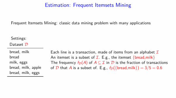
Estimation: Frequent Itemsets Mining

Frequent Itemsets Mining: classic data mining problem with many applications

Settings:Dataset D

bread, milkbreadmilk, eggsbread, milk, applebread, milk, eggs

Each line is a transaction, made of items from an alphabet IAn itemset is a subset of I. E.g., the itemset {bread,milk}The frequency fD(A) of A ™ I in D is the fraction of transactionsof D that A is a subset of. E.g., fD({bread,milk}) = 3/5 = 0.6

Frequent Itemsets Mining

Given a dataset D of transactions D find the k most frequent itemsets.

Exact algorithms are time and space expensive

Can we obtain a good approximation from a sample?

Problem: Rigorous approach that identifies the top frequent itemsets must have someestimate of all possible itemsets (exponential number)

Uniform Convergence

Data analysis through sampling requires simultaneous evaluations of many sets/events

Need sample that approximates/detects all relevant events (uniform convergence)

The union bound is too loose – events are not disjoint

VC-dimension and Rademacher averages allow us to obtain better bounds based onspecific properties of the collection of events

Vapnik–Chervonenkis (VC) - Dimension

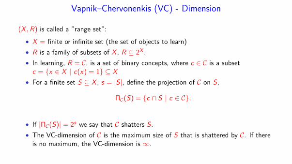
(X , R) is called a ”range set”:• X = finite or infinite set (the set of objects to learn)• R is a family of subsets of X , R ™ 2X .• In learning, R = C, is a set of binary concepts, where c œ C is a subset

c = {x œ X | c(x) = 1} ™ X• For a finite set S ™ X , s = |S|, define the projection of C on S,

�C(S) = {c fl S | c œ C}.

• If |�C(S)| = 2s we say that C shatters S.• The VC-dimension of C is the maximum size of S that is shattered by C. If there

is no maximum, the VC-dimension is Œ.

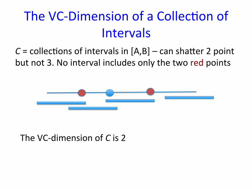
The VC‐Dimension of a Collec9on of 

Intervals 

C = collec9ons of intervals in [A,B] – can shauer 2 point  but not 3. No interval includes only the two red points  

The VC‐dimension of C is 2 

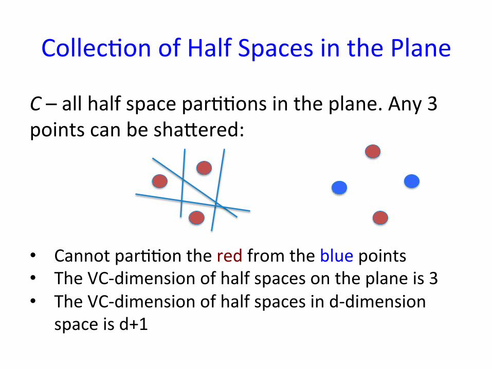
Collec9on of Half Spaces in the Plane 

C – all half space par99ons in the plane. Any 3 points can be shauered: 

 

•  Cannot par99on the red from the blue points 

•  The VC‐dimension of half spaces on the plane is 3 

•  The VC‐dimension of half spaces in d‐dimension 

space is d+1 

Convex Bodies in the Plane 

•  C – all convex bodies on the plane  

Any subset of the point can be included in a convex body.  

The VC‐dimension of C is � 

Questions?

Learning a Classification

TheoremLet C be a concept class with VC-dimension d then C is PAC learnable with

m = O(d‘

ln d‘

+ 1‘

ln 1”

)

samples.

The sample size is not a function of the number of concepts, or the size of the domain!

Sauer’s LemmaVC-dinension is a measure of the complexity (or expressiveness) of a range space - howmany di�erent classification it defines on n elements.For a finite set S ™ X , s = |S|, define the projection of R on S,

�R

(S) = {r fl S | r œ R}.

TheoremLet (X , R) be a range space with VC-dimension d, for S ™ X, such that |S| = n,

|�R

(S)| =dÿ

i=0

Ani

B

Æ nd .

The range space defines up to 2d classifications for d elements, but no more than nd

for larger sets.

Proof

• By induction on d and (for each d) on n, obvious for d = 0, 1 with any n.• Assume that the claim holds for all |S Õ| Æ n ≠ 1 and d Õ Æ d ≠ 1 and let |S| = n.• Fix x œ S and let S Õ = S ≠ {x}.

|�R

(S)| = |{r fl S | r œ R}||�

R

(S Õ)| = |{r fl S Õ | r œ R}||�

R(x)

(S Õ)| = |{r fl S Õ | r œ R and x ”œ r and r fi {x} œ R}|

|�R

(S)| = |�R

(S Õ)| + |�R(x)

(S Õ)|

• (S Õ, �R(x)

(S Õ)) has VC-dimension bounded by d ≠ 1. If B is shattered by(S Õ, �

R(x)

(S Õ)) then B fi {x} is shattered by (X , R)

|�R

(S)| Æd≠1ÿ

i=0

An ≠ 1

i

B

+dÿ

i=0

An ≠ 1

i

B

= 1 +dÿ

i=1

!A

n ≠ 1i ≠ 1

B

+A

n ≠ 1i

B"

=dÿ

i=0

Ani

B

Æ (end )d Æ nd

[We use!

n≠1

i≠1

"+

!n≠1

i

"= (n≠1)!

(i≠1)!(n≠i≠1)!

( 1

n≠i

+ 1

i

) =!

n

i

"]

The number of distinct concepts on n elements grows polynomially in theVC-dimension!

‘-net

Let (X , R) be a range space and D a distribution on X .

DefinitionAn ‘-net for a range space (X , R) is a subset S ™ X such that for any r œ R, ifPr(r) Ø ‘ then |S fl r | Ø 1.

TheoremIf (X , R) is a range space with VC-dimension d then a random sample of size

m = O(d‘

ln d‘

+ 1‘

ln 1”

)

is with probability 1 ≠ ” an ‘-net for (X , R).

‘-sample

DefinitionAn Á-sample for a range space (X , R) is a subset N ™ X such that, for any r œ R,

----Pr(r) ≠ |N fl r ||N|

---- Æ Á .

TheoremIf (X , R) is a range space with VC-dimension d then a random sample of size

m = O( 1‘2

(d + ln1”

)

is, with probability 1 ≠ ”, an ‘-sample for (X , R).

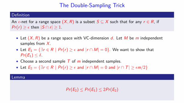
The Double-Sampling TrickDefinitionAn ‘-net for a range space (X , R) is a subset S ™ X such that for any r œ R, ifPr(r) Ø ‘ then |S fl r | Ø 1.

• Let (X , R) be a range space with VC-dimension d . Let M be m independentsamples from X .

• Let E1

= {÷r œ R | Pr(r) Ø ‘ and |r fl M| = 0}. We want to show thatPr(E

1

) Æ ”.• Choose a second sample T of m independent samples.• Let E

2

= {÷r œ R | Pr(r) Ø ‘ and |r fl M| = 0 and |r fl T | Ø ‘m/2}

Lemma

Pr(E2

) Æ Pr(E1

) Æ 2Pr(E2

)

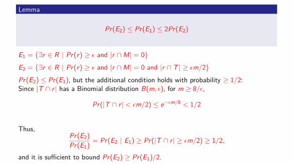
Lemma

Pr(E2

) Æ Pr(E1

) Æ 2Pr(E2

)

E1

= {÷r œ R | Pr(r) Ø ‘ and |r fl M| = 0}

E2

= {÷r œ R | Pr(r) Ø ‘ and |r fl M| = 0 and |r fl T | Ø ‘m/2}

Pr(E2

) Æ Pr(E1

), but the additional condition holds with probability Ø 1/2:Since |T fl r | has a Binomial distribution B(m, ‘), for m Ø 8/‘,

Pr(|T fl r | < ‘m/2) Æ e≠‘m/8 < 1/2

Thus,Pr(E

2

)Pr(E

1

) = Pr(E2

| E1

) Ø Pr(|T fl r | Ø ‘m/2) Ø 1/2,

and it is su�cient to bound Pr(E2

) Ø Pr(E1

)/2.

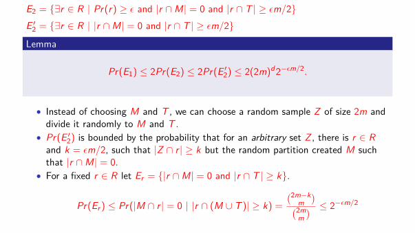
E2

= {÷r œ R | Pr(r) Ø ‘ and |r fl M| = 0 and |r fl T | Ø ‘m/2}E Õ

2

= {÷r œ R | |r fl M| = 0 and |r fl T | Ø ‘m/2}

Lemma

Pr(E1

) Æ 2Pr(E2

) Æ 2Pr(E Õ2

) Æ 2(2m)d2≠‘m/2.

• Instead of choosing M and T , we can choose a random sample Z of size 2m anddivide it randomly to M and T .

• Pr(E Õ2

) is bounded by the probability that for an arbitrary set Z , there is r œ Rand k = ‘m/2, such that |Z fl r | Ø k but the random partition created M suchthat |r fl M| = 0.

• For a fixed r œ R let Er

= {|r fl M| = 0 and |r fl T | Ø k}.

Pr(Er

) Æ Pr(|M fl r | = 0 | |r fl (M fi T )| Ø k) =!

2m≠k

m

"!

2m

m

" Æ 2≠‘m/2

• For a fixed r œ R let Er

= {|r fl M| = 0 and |r fl T | Ø k}.

Pr(Er

) Æ Pr(|M fl r | = 0 | |r fl (M fi T )| Ø k) =!

2m≠k

m

"!

2m

m

" Æ 2≠‘m/2

• For an arbitrary set Z the projection of R on Z gives |�R

(Z )| Æ (2m)d .• Instead of a union bound on |R| we union bound on |�

R

(Z )| Æ (2m)d sets.

Pr(E1

) Æ 2Pr(E Õ2

) Æ 2(2m)d2≠‘m/2 Æ ”

givesm Ø 8d

‘ln 16d

‘+ 4

‘ln 4

”

• Independent of the size of R.

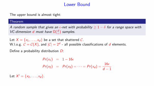
Lower Bound

The upper bound is almost tight:

TheoremA random sample that gives an ‘-net with probability Ø 1 ≠ ” for a range space withVC-dimension d must have �(d

‘ ) samples.

Let X = {x1

, . . . , xd

} be a set that shattered C.W.l.o.g. C = C(X ), and |C| = 2d - all possible classifications of d elements.Define a probability distribution D:

Pr(x1

) = 1 ≠ 16‘

Pr(x2

) = Pr(x3

) = · · · = Pr(xd

) = 16‘

d ≠ 1

Let X Õ = {x2

, . . . , xd

}.

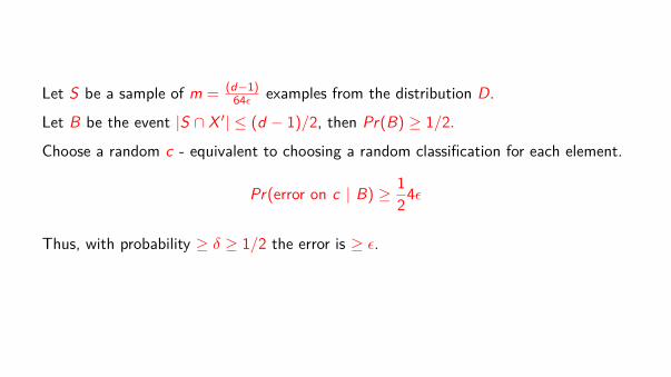
Let S be a sample of m = (d≠1)

64‘ examples from the distribution D.Let B be the event |S fl X Õ| Æ (d ≠ 1)/2, then Pr(B) Ø 1/2.

Choose a random c - equivalent to choosing a random classification for each element.

Pr(error on c | B) Ø 124‘

Thus, with probability Ø ” Ø 1/2 the error is Ø ‘.

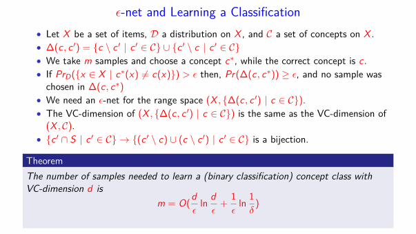
‘-net and Learning a Classification• Let X be a set of items, D a distribution on X , and C a set of concepts on X .• �(c, c Õ) = {c \ c Õ | c Õ œ C} fi {c Õ \ c | c Õ œ C}• We take m samples and choose a concept cú, while the correct concept is c.• If Pr

D

({x œ X | cú(x) ”= c(x)}) > ‘ then, Pr(�(c, cú)) Ø ‘, and no sample waschosen in �(c, cú)

• We need an ‘-net for the range space (X , {�(c, c Õ) | c œ C}).• The VC-dimension of (X , {�(c, c Õ) | c œ C}) is the same as the VC-dimension of

(X , C).• {c Õ fl S | c Õ œ C} æ {(c Õ \ c) fi (c \ c Õ) | c Õ œ C} is a bijection.

TheoremThe number of samples needed to learn a (binary classification) concept class withVC-dimension d is

m = O(d‘

ln d‘

+ 1‘

ln 1”

)

Questions?

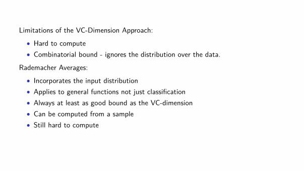
Limitations of the VC-Dimension Approach:• Hard to compute• Combinatorial bound - ignores the distribution over the data.

Rademacher Averages:• Incorporates the input distribution• Applies to general functions not just classification• Always at least as good bound as the VC-dimension• Can be computed from a sample• Still hard to compute

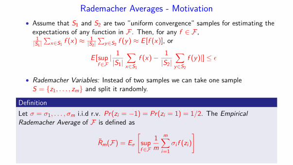
Rademacher Averages - Motivation• Assume that S

1

and S2

are two ”uniform convergence” samples for estimating theexpectations of any function in F . Then, for any f œ F ,

1

|S1

|q

xœS

1

f (x) ¥ 1

|S2

|q

yœS

2

f (y) ¥ E [f (x)], or

E [supf œF

| 1|S

1

|ÿ

xœS

1

f (x) ≠ 1|S

2

|ÿ

yœS

2

f (y)|] Æ ‘

• Rademacher Variables: Instead of two samples we can take one sampleS = {z

1

, . . . , zm

} and split it randomly.

DefinitionLet ‡ = ‡

1

, . . . , ‡m

i.i.d r.v. Pr(zi

= ≠1) = Pr(zi

= 1) = 1/2. The EmpiricalRademacher Average of F is defined as

R̃m

(F) = E‡

C

supf œF

1m

mÿ

i=1

‡i

f (zi

)D

Rademacher Averages - Motivation II

• Assume that F is a collection of {0, 1} classifiers.• A rich concept class F can approximate (correlate) any dichotomy, in particular a

random one - represented by the random variables ‡ = ‡1

, . . . , ‡m

.• Thus, the Rademacher Average

R̃m

(F) = E‡

C

supf œF

1m

mÿ

i=1

‡i

f (zi

)D

represents the richness or expressiveness of the set F .

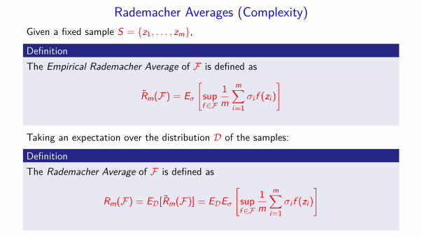
Rademacher Averages (Complexity)Given a fixed sample S = {z

1

, . . . , zm

},

DefinitionThe Empirical Rademacher Average of F is defined as

R̃m

(F) = E‡

C

supf œF

1m

mÿ

i=1

‡i

f (zi

)D

Taking an expectation over the distribution D of the samples:

DefinitionThe Rademacher Average of F is defined as

Rm

(F) = ED[R̃m

(F)] = EDE‡

C

supf œF

1m

mÿ

i=1

‡i

f (zi

)D

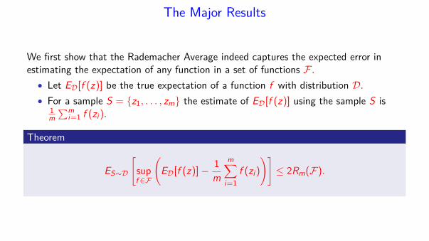
The Major Results

We first show that the Rademacher Average indeed captures the expected error inestimating the expectation of any function in a set of functions F .

• Let ED[f (z)] be the true expectation of a function f with distribution D.• For a sample S = {z

1

, . . . , zm

} the estimate of ED[f (z)] using the sample S is1

m

qm

i=1

f (zi

).

Theorem

ES≥D

C

supf œF

A

ED[f (z)] ≠ 1m

mÿ

i=1

f (zi

)BD

Æ 2Rm

(F).

Proof IdeaPick a second sample S Õ = {z Õ

1

, . . . , z Õm

}.

ES≥D

C

supf œF

A

ED[f (z)] ≠ 1m

mÿ

i=1

f (zi

)BD

= ES≥D

C

supf œF

A

ES

Õ≥D1m

mÿ

i=1

f (z Õi

) ≠ 1m

mÿ

i=1

f (zi

)BD

Æ ES,SÕ≥D

C

supf œF

A1m

mÿ

i=1

f (z Õi

) ≠ 1m

mÿ

i=1

f (zi

)BD

Jensen’s Inequlity

Æ ES,SÕ,‡

C

supf œF

A1m

mÿ

i=1

‡i

(f (zi

) ≠ f (z Õi

)BD

Æ ES,‡

C

supf œF

1m

mÿ

i=1

‡i

(f (zi

)D

+ ES

Õ,‡

C

supf œF

1m

mÿ

i=1

‡i

(f (z Õi

)D

= 2Rm

(F)

Deviation Bound

Assume that that all f œ F satisfy Af

Æ f (z) Æ Af

+ c.Applying Azuma inequality to Doob’s martingale of the functionsup

f œF

1ED[f (z)] ≠ 1

m

qm

i=1

f (zi

)2:

TheoremLet S = {z

1

, . . . , zn

} be a sample from D and let ” œ (0, 1). For all f œ F1 Pr(|ED[f (z)] ≠ 1

m

qm

i=1

f (zi

)| Ø 2Rm

(F) + ‘) Æ e≠2m‘2/c

2

2 Pr(|ED[f (z)] ≠ 1

m

qm

i=1

f (zi

)| Ø 2R̃m

(F) + 2‘) Æ 2e≠2m‘2/c

2

Note that |f (z)| Æ c is equivalent to ≠c Æ f (z) Æ ≠c + 2c.

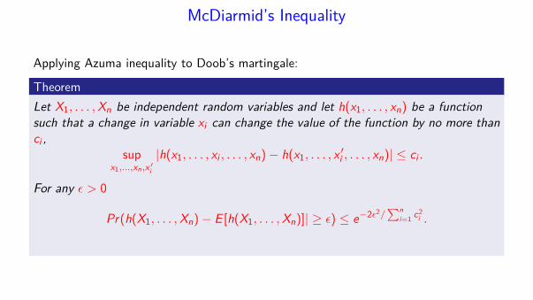
McDiarmid’s Inequality

Applying Azuma inequality to Doob’s martingale:

TheoremLet X

1

, . . . , Xn

be independent random variables and let h(x1

, . . . , xn

) be a functionsuch that a change in variable x

i

can change the value of the function by no more thanc

i

,sup

x

1

,...,xn

,x Õi

|h(x1

, . . . , xi

, . . . , xn

) ≠ h(x1

, . . . , x Õi

, . . . , xn

)| Æ ci

.

For any ‘ > 0

Pr(h(X1

, . . . , Xn

) ≠ E [h(X1

, . . . , Xn

)]| Ø ‘) Æ e≠2‘2/q

n

i=1

c

2

i .

Computing/Estimating Rademacher Averages

Can be estimated from a sample.

TheoremAssume that |F| is finite. Let S = {z

1

, . . . , zm

} be a sample, and assume that

maxf œF

ı̂ıÙ 1m

mÿ

i=1

f 2(zi

) Æ C

thenR̃

m

(F) Æ C

2 log |F|m .

VC-Dimension and Rademacher Averages:From Statistical Learning Theory to Sampling Algorithms

Matteo Riondato1,2 Eli Upfal1

1

Department of Computer Science – Brown University

2

Now at Two Sigma Investments

ECML PKDD ’15 – Porto, September 10, 2015

What time is it?

It’s time to move from Statistical Learning Theory to Sampling Algorithms!

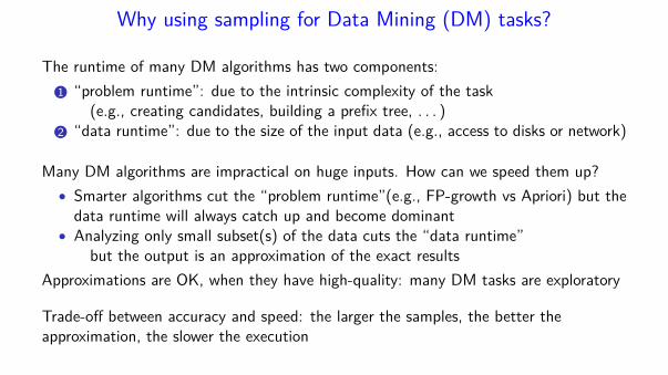
Why using sampling for Data Mining (DM) tasks?

The runtime of many DM algorithms has two components:

1 “problem runtime”: due to the intrinsic complexity of the task(e.g., creating candidates, building a prefix tree, . . . )

2 “data runtime”: due to the size of the input data (e.g., access to disks or network)

Many DM algorithms are impractical on huge inputs. How can we speed them up?

• Smarter algorithms cut the “problem runtime”(e.g., FP-growth vs Apriori) but thedata runtime will always catch up and become dominant

• Analyzing only small subset(s) of the data cuts the “data runtime”but the output is an approximation of the exact results

Approximations are OK, when they have high-quality: many DM tasks are exploratory

Trade-off between accuracy and speed: the larger the samples, the better theapproximation, the slower the execution

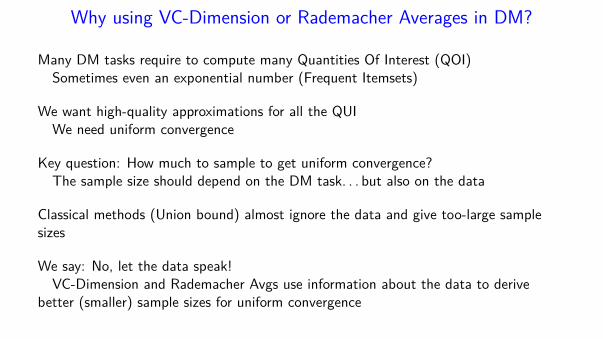
Why using VC-Dimension or Rademacher Averages in DM?

Many DM tasks require to compute many Quantities Of Interest (QOI)Sometimes even an exponential number (Frequent Itemsets)

We want high-quality approximations for all the QUIWe need uniform convergence

Key question: How much to sample to get uniform convergence?The sample size should depend on the DM task. . . but also on the data

Classical methods (Union bound) almost ignore the data and give too-large samplesizes

We say: No, let the data speak!VC-Dimension and Rademacher Avgs use information about the data to derive

better (smaller) sample sizes for uniform convergence

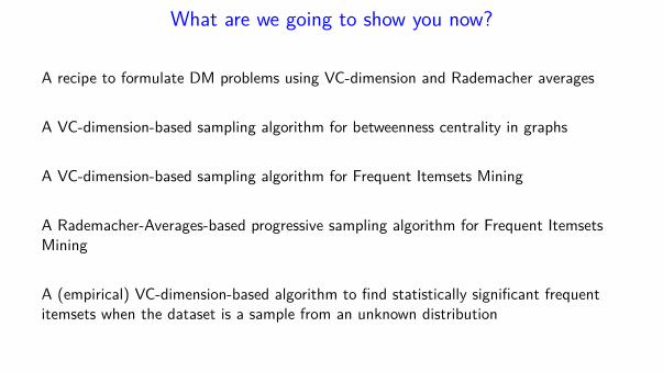
What are we going to show you now?

A recipe to formulate DM problems using VC-dimension and Rademacher averages

A VC-dimension-based sampling algorithm for betweenness centrality in graphs

A VC-dimension-based sampling algorithm for Frequent Itemsets Mining

A Rademacher-Averages-based progressive sampling algorithm for Frequent ItemsetsMining

A (empirical) VC-dimension-based algorithm to find statistically significant frequentitemsets when the dataset is a sample from an unknown distribution

General Recipe

1) Reformulate the DM task as an expectation estimation task:Define the domain U, the family F , and the probability distribution π on U, so that

each QOI is the expectation Eπ[f ] of some f ∈ F w.r.t. π

2) Devise an efficient procedure to sample from U according to πIf the procedure is not efficient, the advantages of sampling are lost

3) Develop an efficient procedure to compute an upper bound to the VC-dimension ofF or to the Rademacher Averages of F on the sample S

If the procedure is not efficient, the advantages of sampling are lost

4) Determine the sample size using the bound and the ε-sample theorem, create thesample, and return the estimation on the sample (running an exact algorithm on thesample or a different procedure)

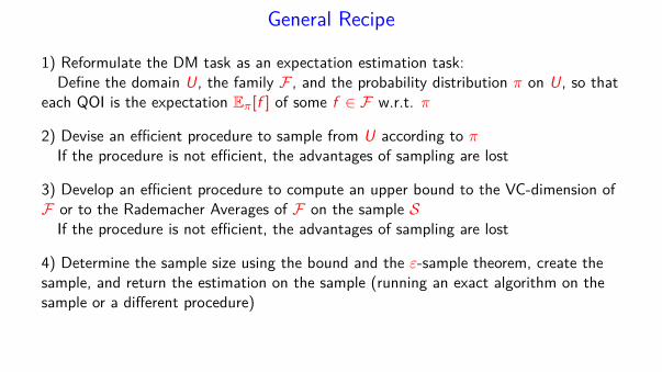
General Recipe

1) Reformulate the DM task as an expectation estimation task:Define the domain U, the family F , and the probability distribution π on U, so that

each QOI is the expectation Eπ[f ] of some f ∈ F w.r.t. π

2) Devise an efficient procedure to sample from U according to πIf the procedure is not efficient, the advantages of sampling are lost

3) Develop an efficient procedure to compute an upper bound to the VC-dimension ofF or to the Rademacher Averages of F on the sample S

If the procedure is not efficient, the advantages of sampling are lost

4) Determine the sample size using the bound and the ε-sample theorem, create thesample, and return the estimation on the sample (running an exact algorithm on thesample or a different procedure)

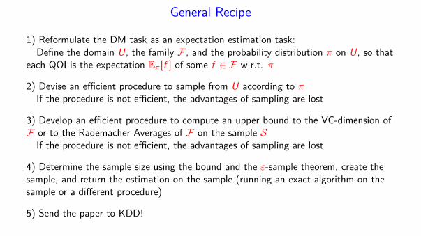
5) Send the paper to KDD!

Application 1: Betweenness Centrality

VC-Dimension-based sampling algorithm for Node Betweenness Centrality[R. and Kornaropoulos, WSDM 2014, DMKD 2015]

What vertices in a graph are important?

Betweenness centrality is one measure of vertex importanceRoughly, it is the fraction of Shortest Paths (SP) in a graph that go through a vertex

Let G = (V , E ), |V | = n, |E | = m. The betweenness centrality of v ∈ V is:

b(v) =1

n(n − 1)︸ ︷︷ ︸

normalization

∑

puw ∈SG

1Tv (puw )

σuw︸ ︷︷ ︸

∈[0,1]

where:

• SG : set of all SPs in G• Suw : set of all SPs from u to w (Suw ⊆ SG , |Suw | = σuw )• Tv : {p ∈ SG : v ∈ Int(p)}

How to compute betweenness centrality?

Naïve algorithm: All Pairs SP computation, followed by aggregationAggregation dominates runtime, Θ(n3)

[Brandes 2001]: Perform aggregation after each Single-Source SP (SSSP) computationRuntime: O(nm) (unweighted G), O(nm + n2 log n) (weighted G)

This is is still too much for graphs with n = 109, m = 1010

Possible solution: perform fewer SPs computations by samplingWe get approximate results, but that’s OK!

What kind of approximation do we want ? What should we sample and how much?

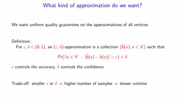
What kind of approximation do we want?

We want uniform quality guarantees on the approximations of all vertices

Definition:For ε, δ ∈ (0, 1), an (ε, δ)-approximation is a collection {b̃(v), v ∈ V } such that

Pr(∃v ∈ V : |b̃(v)− b(v)| > ε) < δ

ε controls the accuracy, δ controls the confidence

Trade-off: smaller ε or δ ⇒ higher number of samples ⇒ slower runtime

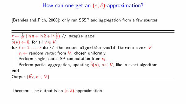
How can one get an (ε, δ)-approximation?

[Brandes and Pich, 2008]: only run SSSP and aggregation from a few sources

r ← 1ε2

(

ln n + ln 2 + ln 1δ

)

// sample size

b̃(v)← 0, for all v ∈ V

for i ← 1, . . . , r do // the exact algorithm would iterate over V

vi ← random vertex from V , chosen uniformlyPerform single-source SP computation from vi

Perform partial aggregation, updating b̃(u), u ∈ V , like in exact algorithm

end

Output {b̃v , v ∈ V }

Theorem: The output is an (ε, δ)-approximation

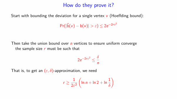
How do they prove it?

Start with bounding the deviation for a single vertex v (Hoeffding bound):

Pr(|b̃(v)− b(v)| > ε) ≤ 2e−2rε2

Then take the union bound over n vertices to ensure uniform convergethe sample size r must be such that

2e−2rε2≤

δ

n

That is, to get an (ε, δ)-approximation, we need

r ≥1

2ε2

(

ln n + ln 2 + ln1

δ

)

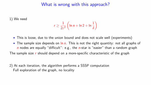
What is wrong with this approach?

1) We need

r ≥1

2ε2

(

ln n + ln 2 + ln1

δ

)

• This is loose, due to the union bound and does not scale well (experiments)

• The sample size depends on ln n. This is not the right quantity: not all graphs ofn nodes are equally “difficult”: e.g., the n-star is “easier” than a random graph

The sample size r should depend on a more-specific characteristic of the graph

2) At each iteration, the algorithm performs a SSSP computationFull exploration of the graph, no locality

How can we improve the sample size?

[R. and Kornaropoulos, 2014] present an algorithm that:

1) uses a sample size which depends on the vertex-diameter, a characteristic quantityof the graph. The derivation uses VC-dimension

2) samples SPs according to a specific, non-uniform distribution over SG . For eachsample, it performs a single s − t SP computation

• More locality: fewer edges touched than single-source SP

• Can use bidirectional search / A*, . . .

What is the algorithm?

VD(G)← vertex-diameter of G // stay tuned!

r ← 12ε2 (⌊log2(VD(G)− 2⌋) + 1 + ln(1/δ)) // sample size

b̃(v)← 0, for all v ∈ V

for i ← 1 . . . , r do

(u, v)← random pair of different vertices, chosen uniformlySuv ← all SPs from u to v // Dijkstra, trunc. BFS, ...

p ← random element of Suv , chosen uniformly // not uniform over SG

b̃(w)← b̃(w) + 1/r , for all w ∈ Int(p) // update only nodes along p

end

Output {b̃(v), v ∈ V }

Theorem: The output {b̃(v), v ∈ V } is an (ε, δ)-approximation

How can we prove the correctness?

We want to prove that the output {b̃(v), v ∈ V } is an (ε, δ)-approximation

Let’s apply the recipe!

1 Define betweenness centrality computation as a expectation estimation problem(domain U, family F , distribution π)

2 Show that the algorithm efficiently samples according to π

3 Show how to efficiently compute an upper bound to the VC-dimensionBonus: show tightness of bound

4 Apply the VC-dimension sampling theorem

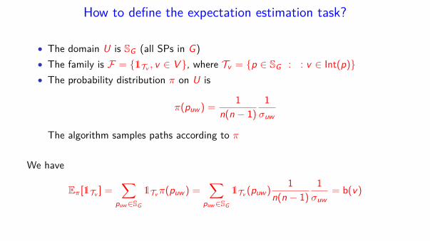
How to define the expectation estimation task?

• The domain U is SG (all SPs in G)

• The family is F = {1Tv , v ∈ V }, where Tv = {p ∈ SG : : v ∈ Int(p)}

• The probability distribution π on U is

π(puw ) =1

n(n − 1)

1

σuw

The algorithm samples paths according to π

We have

Eπ[1Tv ] =∑

puw ∈SG

1Tv π(puw ) =∑

puw ∈SG

1Tv (puw )1

n(n − 1)

1

σuw= b(v)

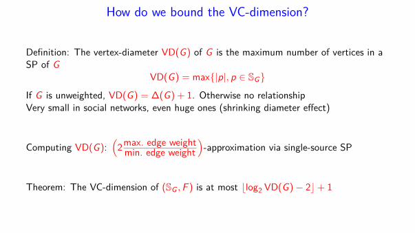
How do we bound the VC-dimension?

Definition: The vertex-diameter VD(G) of G is the maximum number of vertices in aSP of G

VD(G) = max{|p|, p ∈ SG}

If G is unweighted, VD(G) = ∆(G) + 1. Otherwise no relationshipVery small in social networks, even huge ones (shrinking diameter effect)

Computing VD(G):(

2max. edge weightmin. edge weight

)

-approximation via single-source SP

Theorem: The VC-dimension of (SG , F ) is at most ⌊log2 VD(G)− 2⌋+ 1

Let’s prove it!

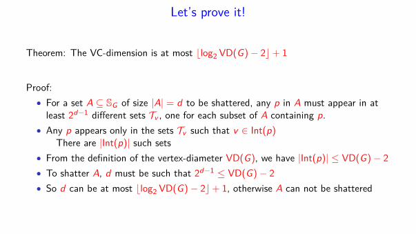
Theorem: The VC-dimension is at most ⌊log2 VD(G)− 2⌋+ 1

Proof:

• For a set A ⊆ SG of size |A| = d to be shattered, any p in A must appear in atleast 2d−1 different sets Tv , one for each subset of A containing p.

• Any p appears only in the sets Tv such that v ∈ Int(p)There are |Int(p)| such sets

• From the definition of the vertex-diameter VD(G), we have |Int(p)| ≤ VD(G)− 2

• To shatter A, d must be such that 2d−1 ≤ VD(G)− 2

• So d can be at most ⌊log2 VD(G)− 2⌋+ 1, otherwise A can not be shattered

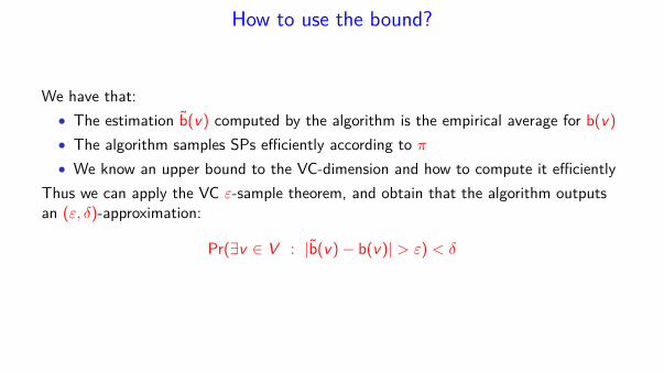
How to use the bound?

We have that:

• The estimation b̃(v) computed by the algorithm is the empirical average for b(v)

• The algorithm samples SPs efficiently according to π

• We know an upper bound to the VC-dimension and how to compute it efficiently

Thus we can apply the VC ε-sample theorem, and obtain that the algorithm outputsan (ε, δ)-approximation:

Pr(∃v ∈ V : |b̃(v)− b(v)| > ε) < δ

Is the bound to the VC-dimension tight?

Yes! There is a class of graphs with VC-dimension exactly ⌊log2 VD(G)− 2⌋+ 1The Concertina Graph Class (Gi)i∈N:

vl vrG1

vl vr

G2

vl vr

G3

vl vr

G4

Theorem: The VC-dimension of (SGi, F ) is ⌊log2 VD(G)− 2⌋+ 1 = i

Proof Intuition: The middle vertices are internal to a lot of SPs

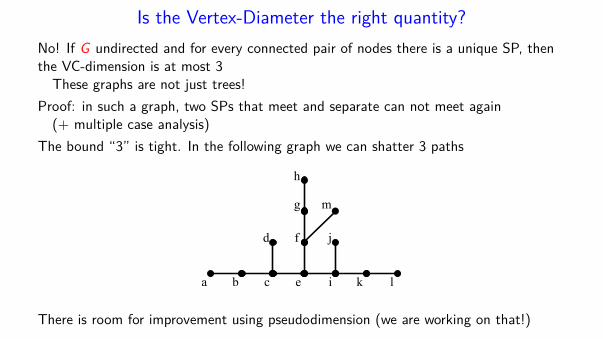
Is the Vertex-Diameter the right quantity?

No! If G undirected and for every connected pair of nodes there is a unique SP, thenthe VC-dimension is at most 3

These graphs are not just trees!

Proof: in such a graph, two SPs that meet and separate can not meet again(+ multiple case analysis)

The bound “3” is tight. In the following graph we can shatter 3 paths

a b c e i k l

d f

g

h

j

m

There is room for improvement using pseudodimension (we are working on that!)

What about directed graphs?

Does a similar result also hold for directed graphs with unique SP?Not for the same constant 3. We built a graph with unique SPs between all

connected nodes and we can shatter a set of 4 SPs

Yes, finding counterexamples is messy. . .

Does it hold for a different constant?We do not know! Maybe you can work on that?

How well does the algorithm perform in practice?

It performs very well!

We tested the algorithm on real graphs (SNAP) and on artificial Barabasi-Albertgraphs, to evalue its accuracy, speed, and scalability

Results: It blows away the exact algorithm and the union-bound-based samplingalgorithm

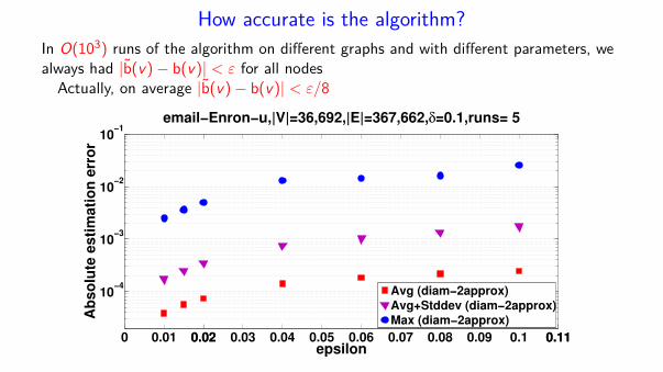
How accurate is the algorithm?

In O(103) runs of the algorithm on different graphs and with different parameters, wealways had |b̃(v)− b(v)| < ε for all nodes

Actually, on average |b̃(v)− b(v)| < ε/8

0 0.01 0.020.02 0.04 0.05 0.06 0.07 0.08 0.09 0.1 0.110.110.03

10−4

10−3

10−2

10−1

epsilon

Ab

so

lute

es

tim

ati

on

err

or

email−Enron−u,|V|=36,692,|E|=367,662,δ=0.1,runs= 5

Avg (diam−2approx)Avg+Stddev (diam−2approx)Max (diam−2approx)

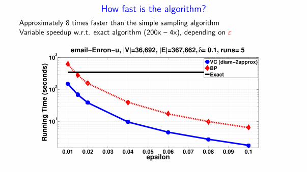
How fast is the algorithm?

Approximately 8 times faster than the simple sampling algorithmVariable speedup w.r.t. exact algorithm (200x – 4x), depending on ε

0.01 0.02 0.03 0.04 0.05 0.06 0.07 0.08 0.09 0.1

101

102

103

epsilon

Ru

nn

ing

Tim

e (

se

co

nd

s)

email−Enron−u, |V|=36,692, |E|=367,662, δ= 0.1, runs= 5

VC (diam−2approx)BPExact

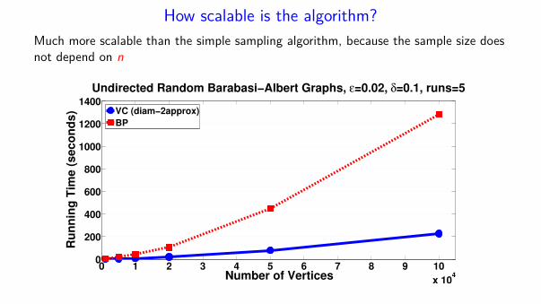
How scalable is the algorithm?

Much more scalable than the simple sampling algorithm, because the sample size doesnot depend on n

0 1 2 3 4 5 6 7 8 9 10

x 104

0

200

400

600

800

1000

1200

1400

Number of Vertices

Ru

nn

ing

Tim

e (

se

co

nd

s)

Undirected Random Barabasi−Albert Graphs, ε=0.02, δ=0.1, runs=5

VC (diam−2approx)

BP

Conclusions (Betweenness Centrality)

We showed a sampling algorithm for betweenness centrality approximation that givesprobabilistic guarantees on the quality of the approximation for all the vertices

The algorithm samples SPs according to a well-defined distribution, and the analysisrelies on VC-dimension, which is bounded by the Vertex Diameter, a characteristicquantity of the graph that is small in real networks

The use of VC-dimension makes the algorithm much faster and more scalable thanprevious sampling approaches and than the exact algorithm

Questions?

Application 2: Frequent Itemsets Mining (FIM)

VC-Dimension-based sampling algorithm for FIM[R. and U., ECML PKDD 2012, TKDD 2014]

Rademacher Averages-based sampling algorithm for FIM[R. and U., KDD 2015]

Empirical-VC-dimension-based algorithm for finding statistically significant FIs[R. and Vandin, SDM 2014]

What is Frequent Itemsets Mining (FIM)?

Frequent Itemsets Mining: classic data mining problem with many applications

Settings:

Dataset D

bread, milkbreadmilk, eggsbread, milk, applebread, milk, eggs

Each line is a transaction, made of items from an alphabet IAn itemset is a subset of I. E.g., the itemset {bread,milk}The frequency fD(A) of A ⊆ I in D is the fraction of transactionsof D that A is a subset of. E.g., fD({bread,milk}) = 3/5 = 0.6

Problem: Frequent Itemsets Mining (FIM)Given θ ∈ [0, 1] find (i.e., mine) all itemsets A ⊆ I with fD(A) ≥ θI.e., compute the set FI(D, θ) = {A ⊆ I : fD(A) ≥ θ}

There exist exact algorithms for FI mining (Apriori, FP-Growth, . . . )

How to make FI mining faster?

Exact algorithms for FI mining do not scale with |D| (no. of transactions):They scan D multiple times: painfully slow when accessing disk or network

How to get faster? We could develop faster exact algorithms (difficult) or. . .. . . only mine random samples of D that fit in main memory

Trading off accuracy for speed: we get an approximation of FI(D, θ) but we get it fastApproximation is OK: FI mining is an exploratory task (the choice of θ is also often

quite arbitrary)

Key question: How much to sample to get an approximation of given quality?

How to define an approximation of the FIs?

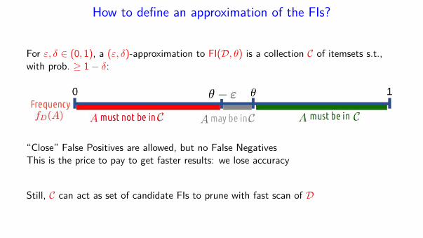
For ε, δ ∈ (0, 1), a (ε, δ)-approximation to FI(D, θ) is a collection C of itemsets s.t.,with prob. ≥ 1− δ:

“Close” False Positives are allowed, but no False NegativesThis is the price to pay to get faster results: we lose accuracy

Still, C can act as set of candidate FIs to prune with fast scan of D

What do we really need?

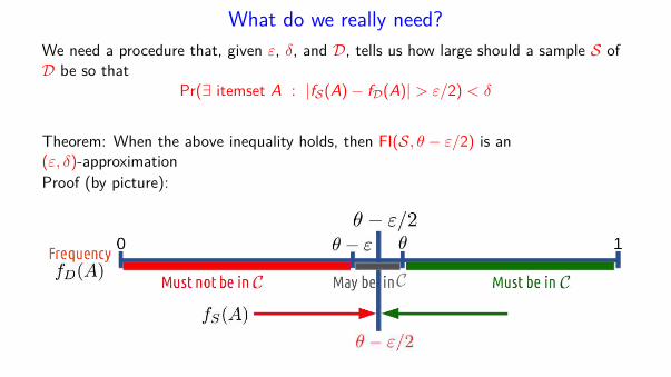
We need a procedure that, given ε, δ, and D, tells us how large should a sample S ofD be so that

Pr(∃ itemset A : |fS(A)− fD(A)| > ε/2) < δ

Theorem: When the above inequality holds, then FI(S, θ − ε/2) is an(ε, δ)-approximationProof (by picture):

Where does the union bound fall short?

For any itemset A, |S|fS(A) has a Binomial distribution with expectation |S|fD(A)We can use the Chernoff bound and have

Pr(|fS(A)− fD(A)| > ε/2) ≤ 2e−|S|ε2/12

We then apply the union bound over all the itemsets to obtain uniform convergenceThere are 2|I| itemsets, a priori. We need

2e−|S|ε2/12 ≤ δ/2|I|

Thus

|S| ≥12

ε2

(

|I| + ln 2 + ln1

δ

)

The sample size depends on |I| but I can be very largeE.g., all the products sold by Amazon, all the pages on the Web, . . .

We need a smaller sample size that depends on some characteristic quantity of D

How do we get a smaller sample size?

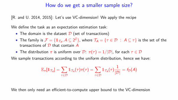
[R. and U. 2014, 2015]: Let’s use VC-dimension! We apply the recipe

We define the task as an expectation estimation task:

• The domain is the dataset D (set of transactions)

• The family is F = {1TA, A ⊆ 2I}, where TA = {τ ∈ D : A ⊆ τ} is the set of the

transactions of D that contain A

• The distribution π is uniform over D: π(τ) = 1/|D|, for each τ ∈ D

We sample transactions according to the uniform distribution, hence we have:

Eπ[1TA] =

∑

τ∈D

1TA(τ)π(τ) =

∑

τ∈D

1TA(τ)

1

|D|= fD(A)

We then only need an efficient-to-compute upper bound to the VC-dimension

How do we bound the VC-dimension?

Enters the d-index of a dataset D!

The d-index d of a dataset D is the maximum integer such that D contains at least d

different transactions of length at least d

Example: The following dataset has d-index 3

bread beer milk coffeechips coke pastabread coke chipsmilk coffeepasta milk

It is similar but not equal to the h-index for published authors

It can be computed easily with a single scan of the dataset

Theorem: The VC-dimension is less or equal to the d-index d of D

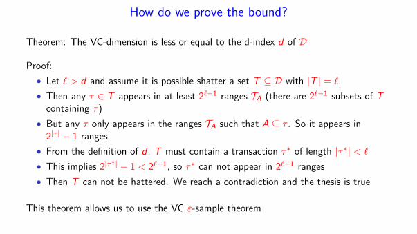
How do we prove the bound?

Theorem: The VC-dimension is less or equal to the d-index d of D

Proof:

• Let ℓ > d and assume it is possible shatter a set T ⊆ D with |T | = ℓ.

• Then any τ ∈ T appears in at least 2ℓ−1 ranges TA (there are 2ℓ−1 subsets of T

containing τ)

• But any τ only appears in the ranges TA such that A ⊆ τ . So it appears in2|τ | − 1 ranges

• From the definition of d , T must contain a transaction τ∗ of length |τ∗| < ℓ

• This implies 2|τ∗| − 1 < 2ℓ−1, so τ∗ can not appear in 2ℓ−1 ranges

• Then T can not be hattered. We reach a contradiction and the thesis is true

This theorem allows us to use the VC ε-sample theorem

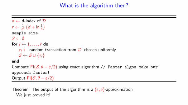
What is the algorithm then?

d ← d-index of Dr ← 1

ε2

(

d + ln 1δ

)

sample size

S ← ∅for i ← 1, . . . , r do

τi ← random transaction from D, chosen uniformlyS ← S ∪ {τi}

end

Compute FI(S, θ − ε/2) using exact algorithm // Faster algos make our

approach faster!

Output FI(S, θ − ε/2)

Theorem: The output of the algorithm is a (ε, δ)-approximationWe just proved it!

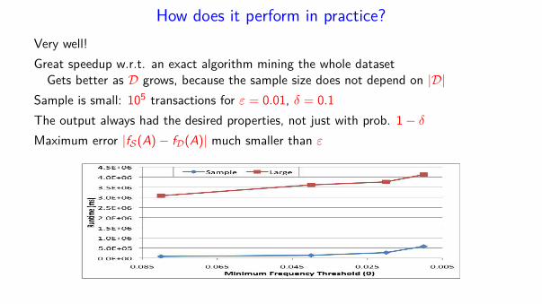
How does it perform in practice?

Very well!

Great speedup w.r.t. an exact algorithm mining the whole datasetGets better as D grows, because the sample size does not depend on |D|

Sample is small: 105 transactions for ε = 0.01, δ = 0.1

The output always had the desired properties, not just with prob. 1− δ

Maximum error |fS(A)− fD(A)| much smaller than ε

Questions?

. . . so all is well, right?

There are some issues with the VC-dimension approach:

• Computing the d-index requires a full scan of the datasetThis can still be expensive. Can we avoid it?

• The definition of the d-index depends on ’extreme’ transactions:Maximum d such that D contains at least d transactions of length at least d

This make the sample size too dependent on outliers. Can we do better?• The VC-approach can not handle the following scenario:

• We are given only a random sample S of D (no access to the dataset)• We are asked how good of an approximation we can get from this sample: given

some δ, what is the minimum ε such that S is a (ε, δ)-approximation?

Can we let the sample tells us how good it is?

[R. and U., 2015]: Let the sample speak! We use Progressive Random Sampling andRademacher Averages to solve the above issues

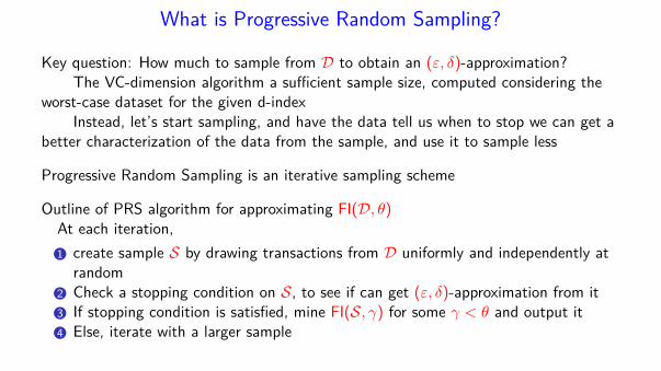
What is Progressive Random Sampling?

Key question: How much to sample from D to obtain an (ε, δ)-approximation?The VC-dimension algorithm a sufficient sample size, computed considering the

worst-case dataset for the given d-indexInstead, let’s start sampling, and have the data tell us when to stop we can get a

better characterization of the data from the sample, and use it to sample less

Progressive Random Sampling is an iterative sampling scheme

Outline of PRS algorithm for approximating FI(D, θ)At each iteration,

1 create sample S by drawing transactions from D uniformly and independently atrandom

2 Check a stopping condition on S, to see if can get (ε, δ)-approximation from it3 If stopping condition is satisfied, mine FI(S, γ) for some γ < θ and output it4 Else, iterate with a larger sample

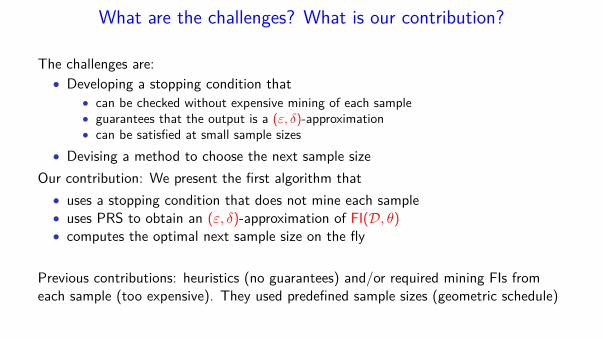
What are the challenges? What is our contribution?

The challenges are:• Developing a stopping condition that

• can be checked without expensive mining of each sample• guarantees that the output is a (ε, δ)-approximation• can be satisfied at small sample sizes

• Devising a method to choose the next sample size

Our contribution: We present the first algorithm that

• uses a stopping condition that does not mine each sample• uses PRS to obtain an (ε, δ)-approximation of FI(D, θ)• computes the optimal next sample size on the fly

Previous contributions: heuristics (no guarantees) and/or required mining FIs fromeach sample (too expensive). They used predefined sample sizes (geometric schedule)

What do we really need?We need an e�cient procedure that, given a sample S of D, computes a value ÷ s.t.

Pr

supA™I

|fD(A) ≠ fS(A)| Æ ÷

!Ø 1 ≠ ”

Then the stopping condition just tests if ÷ Æ Á/2Theorem: If ÷ Æ Á/2, then FI(S, ◊ ≠ Á/2| {z }

“

) is an (Á, ”)-approximation to FI(D, I, ◊)

Proof (by picture) Like the one for the VC-dimension algorithm

How to compute ÷? Using Rademacher Averages!

What are Rademacher Averages? (Quick recall)

A measure of complexity of the task w.r.t. sampling (VC-dimension on steroids)Definition is hairy: Let S = {τ1, . . . , τ|S|}, the Rademacher Average on S is

R(S) = Eσ

⎡

⎣supA⊆I

1

ℓ

|S|∑

j=1

σjφA(τj) | S

⎤

⎦

where the σi are Rademacher rv’s and φA(τi) = 1τj (A)The important part: R(S) is a sample-dependent quantity and we have:

Pr

⎛

⎜⎜⎜⎝

supA⊆I

|fD(A)− fS(A)| ≤ 2R(S) +

√

2 ln(2/δ)

|S|︸ ︷︷ ︸

η

⎞

⎟⎟⎟⎠≥ 1− δ

We develop a method to efficiently compute an upper bound to R(S)So we can compute η and efficiently check the stopping condition “η ≤ ε/2?”

How can we bound the Rademacher average? (high level picture)

We compute an upper bound to the distribution of the frequencies in S of the ClosedItemsets (CIs) in S (An itemset is closed iff none of its supersets has the samefrequency)

Connection with the CIs: supA⊆I

|fD(A)− fS(A)| = supA∈CIs

|fD(A)− fS(A)|

Efficiency Constraint: use only information that can be obtained with a single scan of S

How:

1 We use the frequency of the single items and the lengths of the transactions todefine a (conceptual) partitioning of the CIs into classes, and to compute upperbounds to the size of each class and to the frequencies of the CIs in the class

2 We use these bounds to compute an upper bound to R(S) by minimizing a convexfunction in R+ (no constraints)

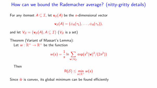
How can we bound the Rademacher average? (nitty-gritty details)

For any itemset A ⊆ I, let vS(A) be the n-dimensional vector

vS(A) = (φA(τ1), . . . , φA(τn)),

and let VS = {vS(A), A ⊆ I} (VS is a set)

Theorem (Variant of Massart’s Lemma):Let w : R+ → R+ be the function

w(s) =1

sln∑

v∈VS

exp(s2∥v∥2/(2n2))

ThenR(S) ≤ min

s∈R+w(s)

Since w̃ is convex, its global minimum can be found efficiently

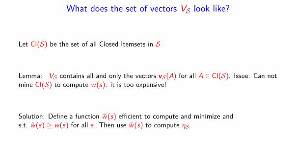
What does the set of vectors VS look like?

Let CI(S) be the set of all Closed Itemsets in S

Lemma: VS contains all and only the vectors vS(A) for all A ∈ CI(S). Issue: Can notmine CI(S) to compute w(s): it is too expensive!

Solution: Define a function w̃(s) efficient to compute and minimize ands.t. w̃(s) ≥ w(s) for all s. Then use w̃(s) to compute ηS

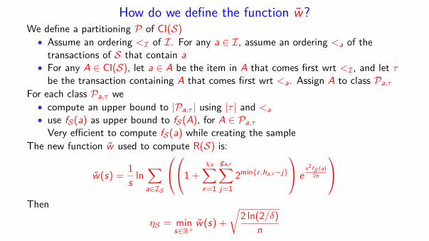
How do we define the function w̃?We define a partitioning P of CI(S)

• Assume an ordering <I of I. For any a ∈ I, assume an ordering <a of thetransactions of S that contain a

• For any A ∈ CI(S), let a ∈ A be the item in A that comes first wrt <I , and let τbe the transaction containing A that comes first wrt <a. Assign A to class Pa,τ

For each class Pa,τ we• compute an upper bound to |Pa,τ | using |τ | and <a

• use fS(a) as upper bound to fS(A), for A ∈ Pa,τ

Very efficient to compute fS(a) while creating the sampleThe new function w̃ used to compute R(S) is:

w̃(s) =1

sln∑

a∈IS

⎛

⎝

⎛

⎝1 +χa∑

r=1

ga,r∑

j=1

2min{r ,ha,r −j}

⎞

⎠ es2fS (a)

2n

⎞

⎠

Then

ηS = mins∈R+

w̃(s) +

√

2 ln(2/δ)

n

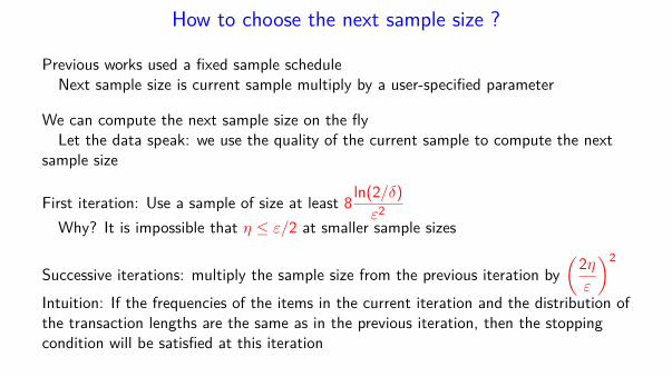
How to choose the next sample size ?

Previous works used a fixed sample scheduleNext sample size is current sample multiply by a user-specified parameter

We can compute the next sample size on the flyLet the data speak: we use the quality of the current sample to compute the next

sample size

First iteration: Use a sample of size at least 8ln(2/δ)

ε2

Why? It is impossible that η ≤ ε/2 at smaller sample sizes

Successive iterations: multiply the sample size from the previous iteration by

(2η

ε

)2

Intuition: If the frequencies of the items in the current iteration and the distribution ofthe transaction lengths are the same as in the previous iteration, then the stoppingcondition will be satisfied at this iteration

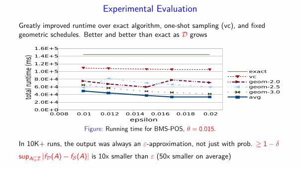
Experimental Evaluation

Greatly improved runtime over exact algorithm, one-shot sampling (vc), and fixedgeometric schedules. Better and better than exact as D grows

0.008 0.01 0.012 0.014 0.016 0.018 0.020.0E+0

2.0E+4

4.0E+4

6.0E+4

8.0E+4

1.0E+5

1.2E+5

1.4E+5

1.6E+5

exactvcgeom-2.0geom-2.5geom-3.0avg

epsilon

tota

l run

time (

ms)

Figure: Running time for BMS-POS, θ = 0.015.

In 10K+ runs, the output was always an ε-approximation, not just with prob. ≥ 1− δ

supA⊆I |fD(A)− fS(A)| is 10x smaller than ε (50x smaller on average)

How does it compare to the VC-dimension algorithm?

Given a sample S and some δ ∈ (0, 1), what is the smallest ε such that FI(S, θ − ε/2)is a (ε, δ)-approximation?

0.0E+0 2.0E+6 4.0E+60

0.02

0.04

0.06

0.08 kosarakVC

This work

sample size

epsi

lon

0.0E+0 2.0E+6 4.0E+60

0.01

0.02

0.03

0.04 accidents

VCThis work

sample size

epsi

lon

Note that this comparison is unfavorable to our algorithm: as we are allowing theVC-dimension approach to compute the d-index of D (but we don’t have access to D!)

We strongly believe that this is because we haven’t optimized all the aspects of thebound to the Rademacher average. Once we do it, the Rademacher avg approach willmost probably always be better

Recap

We show two algorithms for approximating the FIs using sampling

One uses VC-dimension and the d-index of the dataset to compute the sample size.This approach has some drawback

The second uses progressive sampling, with a stopping condition based on Rademacheraverages, and solves most of the issues with the VC-approach

Questions?

Let’s look at the data differently

The dataset D should (often) not be considered a perfect representation of realityRather, it is a sample from an unknown generative process

Reality is partially and noisily represented in the datasetItemsets may be frequent in D only due to random fluctuations

The real goal of mining is understanding the unknown generative process We shouldmine are the itemsets that have high probability of being generated: the True FrequentItemsets [R. and Vandin, 2014]

What are the True Frequent Itemsets?

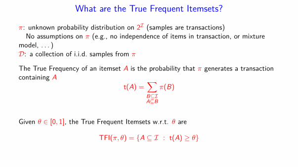
π: unknown probability distribution on 2I (samples are transactions)No assumptions on π (e.g., no independence of items in transaction, or mixture

model, . . . )D: a collection of i.i.d. samples from π

The True Frequency of an itemset A is the probability that π generates a transactioncontaining A

t(A) =∑

B⊆IA⊆B

π(B)

Given θ ∈ [0, 1], the True Frequent Itemsets w.r.t. θ are

TFI(π, θ) = {A ⊆ I : t(A) ≥ θ}

What can we really do?

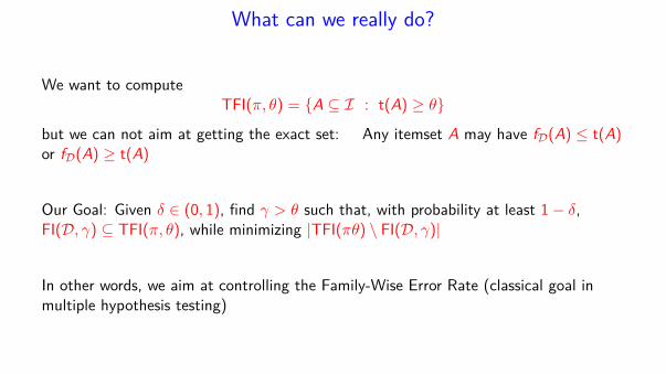
We want to computeTFI(π, θ) = {A ⊆ I : t(A) ≥ θ}

but we can not aim at getting the exact set: Any itemset A may have fD(A) ≤ t(A)or fD(A) ≥ t(A)

Our Goal: Given δ ∈ (0, 1), find γ > θ such that, with probability at least 1− δ,FI(D, γ) ⊆ TFI(π, θ), while minimizing |TFI(πθ) \ FI(D, γ)|

In other words, we aim at controlling the Family-Wise Error Rate (classical goal inmultiple hypothesis testing)

What are we actually looking for?

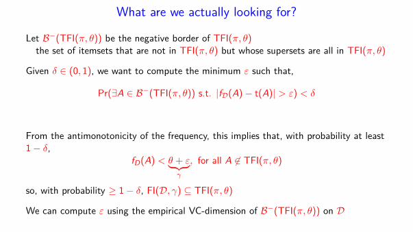
Let B−(TFI(π, θ)) be the negative border of TFI(π, θ)the set of itemsets that are not in TFI(π, θ) but whose supersets are all in TFI(π, θ)

Given δ ∈ (0, 1), we want to compute the minimum ε such that,

Pr(∃A ∈ B−(TFI(π, θ)) s.t. |fD(A)− t(A)| > ε) < δ

From the antimonotonicity of the frequency, this implies that, with probability at least1− δ,

fD(A) < θ + ε︸ ︷︷ ︸

γ

, for all A ̸∈ TFI(π, θ)

so, with probability ≥ 1− δ, FI(D, γ) ⊆ TFI(π, θ)

We can compute ε using the empirical VC-dimension of B−(TFI(π, θ)) on D

What is the empirical VC-dimension?

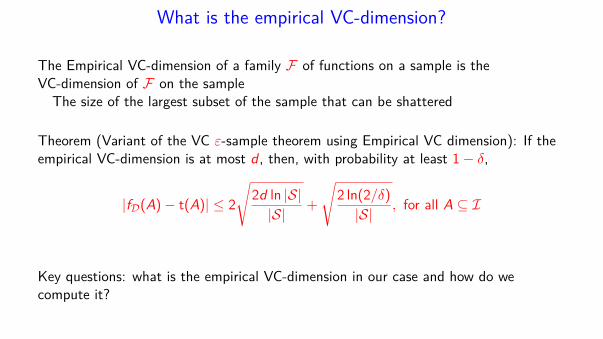
The Empirical VC-dimension of a family F of functions on a sample is theVC-dimension of F on the sample

The size of the largest subset of the sample that can be shattered

Theorem (Variant of the VC ε-sample theorem using Empirical VC dimension): If theempirical VC-dimension is at most d , then, with probability at least 1− δ,

|fD(A)− t(A)| ≤ 2

√

2d ln |S|

|S|+

√

2 ln(2/δ)

|S|, for all A ⊆ I

Key questions: what is the empirical VC-dimension in our case and how do wecompute it?

What is the empirical VC-dimension of B−(TFI(π, θ)) ?

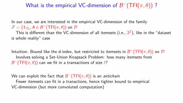
In our case, we are interested in the empirical VC-dimension of the familyF = {1TA

, A ∈ B−(TFI(π, θ)) on DThis is different than the VC-dimension of all itemsets (i.e., 2I), like in the “dataset

is whole reality” case

Intuition: Bound like the d-index, but restricted to itemsets in B−(TFI(π, θ)) on DInvolves solving a Set-Union Knapsack Problem: how many itemsets from

B−(TFI(π, θ)) can we fit in a transactions of size ℓ?

We can exploit the fact that B−(TFI(π, θ)) is an antichain

Fewer itemsets can fit in a tranactions, hence tighter bound to empiricalVC-dimension (but more convoluted computation)

What is the algorithm?

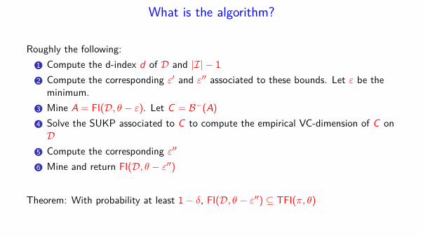
Roughly the following:

1 Compute the d-index d of D and |I|− 1

2 Compute the corresponding ε′ and ε′′ associated to these bounds. Let ε be theminimum.

3 Mine A = FI(D, θ − ε). Let C = B−(A)

4 Solve the SUKP associated to C to compute the empirical VC-dimension of C onD

5 Compute the corresponding ε′′

6 Mine and return FI(D, θ − ε′′)

Theorem: With probability at least 1− δ, FI(D, θ − ε′′) ⊆ TFI(π, θ)

How well does it perform in practice?

Always had FI(D, θ − ε′′) ⊆ TFI(π, θ)Always reported more TFIs than previous approach with Chernoff+Union bound

Conclusions (Empirical VC-dimension)

The techniques and results we presented in the first part of the talk can be used also inthe case where the dataset is a sample from an unknown distribution

Although the empirical VC-dimension is powerful, we believe that a Rademacheraverage approach would give better results also in this case

There is a lot to explore. . .

Questions?

General Conclusions

VC-dimension and Rademacher averages are a great addition to the DM algorithmdesigner toolkit They are

• Powerful

• Game-changing

• Intuitive (at least VC-dim. . . )

• Elegant

• Difficult to compute exactly but relatively easy to bound

• Extremely adaptible to different scenarios

We only scratched the surface and showed a few applicationsThere is much more (differential privacy, noisy datasets, . . . )

Embrace Statistical Learning Theory :-)

Contacts

Tutorial Website: http://bigdata.cs.brown.edu/vctutorial/

Come talk to us!

Matteo Riondato – matteo@twosigma.com

Two Sigma Investmentshttp://matteo.rionda.to – @riondabsd

Eli Upfal – eli@cs.brown.edu

Department of Computer Science – Brown Universityhttp://cs.brown.edu/~eli