Embed Size (px)
Citation preview
VayuAnukulani: Adaptive Memory Networks forAir Pollution Forecasting
Divyam Madaan∗Panjab University
Radhika Dua∗Panjab University
Prerana MukherjeeIIIT Sricity
Brejesh LallIIT Delhi
Abstract—Air pollution is the leading environmental healthhazard globally due to various sources which include factoryemissions, car exhaust and cooking stoves. As a precautionarymeasure, air pollution forecast serves as the basis for takingeffective pollution control measures, and accurate air pollutionforecasting has become an important task. In this paper, weforecast fine-grained ambient air quality information for 5prominent locations in Delhi based on the historical and real-time ambient air quality and meteorological data reported byCentral Pollution Control board. We present VayuAnukulanisystem, a novel end-to-end solution to predict air quality for next24 hours by estimating the concentration and level of different airpollutants including nitrogen dioxide (NO2), particulate matter(PM2.5 and PM10) for Delhi. Extensive experiments on datasources obtained in Delhi demonstrate that the proposed adap-tive attention based Bidirectional LSTM Network outperformsseveral baselines for classification and regression models. Theaccuracy of the proposed adaptive system is ∼ 15− 20% betterthan the same offline trained model. We compare the proposedmethodology on several competing baselines, and show that thenetwork outperforms conventional methods by ∼ 3− 5%.
Index Terms—Air quality, Pollution forecasting, Real time airquality prediction, Deep Learning
I. INTRODUCTION
Due to the rapid urbanization and industrialization, thereis an increase in the number of vehicles, and the burningof fossil fuels, due to which the quality of air is degrading,which is a basic requirement for the survival of all lives onEarth. The rise in the pollution rate has affected people withserious health hazards such as heart disease, lung cancer andchronic respiratory infections like asthma, pneumonia etc. Airpollution has also become a major cause for skin and eyehealth conditions in the country.
One of the most important emerging environmental issuesin the world is air pollution. According to World HealthOrganization (WHO), in 2018, India has 14 out of the 15 mostpolluted cities in the world. The increasing level of pollutantsin ambient air in 2016-2018 has deteriorated the air qualityof Delhi at an alarming rate. All these problems brought usto focus the current study on air quality in Delhi region. Theestablishment of a reasonable and accurate forecasting modelis the basis for forecasting urban air pollution, which caninform government’s policy-making bodies to perform trafficcontrol when the air is polluted at critical levels and people’s
*Equal Contribution
decision making like whether to exercise outdoors or whichroute to follow.
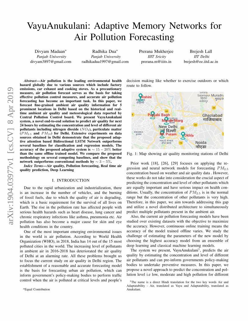
Fig. 1: Map showing air quality monitoring stations of Delhi
Prior work [18], [26], [29] focuses on applying the re-gression and neural network models for forecasting PM2.5
concentration based on weather and air quality data . However,these works do not take into consideration the crucial aspect ofpredicting the concentration and level of other pollutants whichare equally important and have serious impact on health con-ditions. Usually, the concentration of PM2.5 is in the normalrange but the concentration of other pollutants is very high.Therefore, in this paper, we aim towards addressing this gapand utilize a novel distributed architecture to simultaneouslypredict multiple pollutants present in the ambient air.
Also, the current air pollution forecasting models have beenstudied over existing datasets with the objective to maximizethe accuracy. However, continuous online training means theaccuracy of the model trained offline varies. We study thechallenge of estimating the parameters of the new model bychoosing the highest accuracy model from an ensemble ofdeep learning and classical machine learning models.
The system we present, VayuAnukulani1, predicts the airquality by estimating the concentration and level of differentair pollutants and can pre-inform governments policy-makingbodies to undertake preventive measures. In this paper, wepropose a novel approach to predict the concentration and pol-lution level i.e low, moderate and high pollution for different
1The name is a direct Hindi translation for the two key words Air andAdaptatability - Air, translated as Vayu and Adaptatability, translated asAnukulani.
arX
iv:1
904.
0397
7v1
[cs
.CV
] 8
Apr
201
9
air pollutants including nitrogen dioxide (NO2) and particulatematter (PM2.5 and PM10) for 5 different monitoring stationsin Delhi as shown in Fig. 1 (screenshot from our website),considering air quality data, time and meteorological data ofthe past 24 hours. To the best of the author’s knowledge, thiswork is one of the first holistic and empirical research where asingle model predicts multiple pollutants and makes adaptiveupdates to improvise the future predictions.
The key contributions in this work can be summarized as,
1) The proposed approach uses heterogeneous urban datafor capturing both direct (air pollutants) and indirect(meteorological data and time) factors. The model adaptsto a novel distributed architecture in order to simulta-neously model the interactions between these factorsfor leveraging learning of the individual and holisticinfluences on air pollution.
2) We build a novel end-to-end adaptive system that col-lects the pollution data over a period of 1-3 years for 5locations of Delhi, trains two models (forecast/classify)to predict the concentration and classify the pollutionlevel for each pollutant to 2-3 classes (3 classes forPM2.5 and PM10, 2 classes for SO2 and NO2) forthe next 24 hours, and then deploys a new model.
3) We achieve a significant gain of ∼ 15 − 20% accuracywith the proposed adaptive system as compared to thesame offline trained model. The proposed system alsooutperforms several competing baselines and we achievea performance boost of about ∼ 3 − 5% in forecastingof pollution levels and concentration.The remainder of this paper is organized as follows. InSec. II, we discuss the challenges occurring in imple-menting air pollution forecasting system and in Sec. IV,we outline the background description of various deeplearning architectures for temporal forecasting. In Sec.V, we provide a detailed overview of the componentblocks of the proposed architecture for air pollutionforecasting followed by an evaluation of the same inSec. VI. In Sec. VII we provide the details about thedeveloped web application and in Sec. VIII, we concludethe paper.
II. CHALLENGES
Some of the major problems that occur while implementinga prediction system to forecast the concentration and level ofair pollutants are:
• Air pollution varies with time and space. Therefore, it isessential to maintain spatial and temporal granularity inair quality forecasting system.
• The data is often insufficient and inaccurate. Sometimesthe concentration of pollutants is much beyond the per-missible limits.
• Air pollution dataset contains several outliers (the pol-lution increases/decreases significantly all of a sudden),which is mainly due to accidental forest fires, burning ofagricultural wastes and burning of crackers during diwali.
• Air pollution depends on direct (historical air pollutiondata) and indirect factors (like time, meteorological data)and modelling the relationship between these factors isquite complex.
• In order to forecast the concentration and level of airpollutants, it is necessary to collect data for every lo-cation independently as pollution varies drastically withgeographical distance.
• Separate models are deployed for each location andtraining each model regularly is computationally expen-sive. Thus, updating data and training model for eachlocation becomes unmanageable when we deal with manylocations.
In the proposed method, we address the aforementionedchallenges. We train separate models for each location as thepollution varies with varying geographical distance. Hourly airpollution and meteorological data is collected as the pollutionvaries significantly with time. We use various imputationtechniques in order to deal with missing values and performdata preprocessing to select and use only the important featuresfor air pollution prediction as detailed in sec. V-A2.
III. RELATED WORK
In this section we provide a detailed overview of thecontemporary techniques prevalent in the domains which areclosely related to our work and broadly categorize them intothe following categories for temporal forecasting.
A. Handcrafted features based techniques
Traditional handcrafted feature based approaches [18] uti-lize Markovian approaches to predict PM2.5 concentrationusing time series data. Since, Hidden Markov Models (HMMs)suffer from the limitation of short term memory thus failing incapturing the temporal dependencies in prediction problems.To overcome this, authors in [18] highlight a variant of HMMs:hidden semi-Markov models (HSMMs) for PM2.5 concentra-tion prediction by introducing temporal structures into stan-dard HMMs. In [26], authors provide a hybrid frameworkwhich relies on feature reduction followed by a hyperplanebased classifier (Least Square Support Vector Machine) topredict the particulate matter concentration in the ambient air.The generalization ability of the classifier is improvised usingcuckoo search optimization strategy. In [28], authors compareand contrast various neural network based models like Ex-treme Learning Machine, Wavelet Neural Networks, FuzzyNeural Networks, Least Square Support Vector Machines topredict PM2.5 concentration over short term durations. Theydemonstrate the efficacy of Wavelet Neural Networks overthe compared architectures in terms of higher precision andself learning ability. Even meteorological parameters suchas humidity and temperature are considered for evaluation.In [24], authors provide an hourly prediction over PM2.5
concentration depicting multiple change patterns. They trainseparate models over clusters comprising of subsets of thedata utilizing an ensemble of classification and regression treeswhich captures the multiple change pattern in the data.
In contrast to the aligning works [18], [24], [26], [28], inthis paper we capture the long-term temporal dependenciesbetween the data sources collected using both direct as wellas indirect sources and introduce the importance of attentionbased adaptive learning in the memory networks. Apart fromthat, we provide a standalone model to predict various pollu-tants (PM2.5, NO2 and Pm10) over a long period of time infuture (next 24 hours).
B. Deep Learning based techniquesIn recent times, researchers are predominantly utilizing
deep learning based architectures for forecasting expresswayPM2.5 concentration. In [17], the authors devise a novelalgorithm to handle the missing values in the urban data forChina and Hong Kong followed by deep learning paradigmfor air pollution estimation. This enables in predicting theair quality estimates throughout the city thus, curtailing thecost which might be incurred due to setup of sophisticatedair quality monitors. In [21], authors provide a deep neuralnetwork (DNN) model to predict industrial air pollution. Anon-linear activation function in the hidden units in the DNNreduces the vanishing gradient effect. In [15], authors proposeLong Short Term Memory (LSTM) networks to predict futurevalues of air quality in smart cities utilizing the IoT smartcity data. In [16], authors utilize geographical distance andspatiotemporally correlated PM2.5 concentration in a deepbelief network to capture necessary evaluators associated withPM2.5 from latent factors. In [22], authors adopt a DeepAir Learning framework which emphasize on utilizing theinformation embedded in the unlabeled spatio-temporal datafor improving the interpolation and prediction performance.
In this paper, we however predict other pollutants(PM2.5, NO2 and Pm10) which are equally important to scalethe air quality index to an associated harmful level utilizingthe deep learning based paradigm.
C. Wireless networks based techniquesIn [3], authors utilize mobile wireless sensor networks
(MWSN) for generating precise pollution maps based onthe sensor measurement values and physical models whichemulate the phenomenon of pollution dispersion. This worksin a synergistic manner by reducing the errors due to thesimulation runs based on physical models while relying onsensor measurements. However, it would still rely on thedeployment of the sensor nodes. In [14], authors utilize node-to-node calibration, in which at a time one sensor in each chainis directly calibrated against the reference measurements andthe rest are calibrated sequentially while they are deployedand occur in pairs. This deployment reduces the load onsensor relocations and ensures simultaneous calibration anddata collection. In [7], authors propose a framework for airquality estimation utilizing multi-source heterogeneous datacollected from wireless sensor networks.
D. Trends and seasonality assessment based techniquesIn [19], authors present a detailed survey on the trends
of the seasonal variations across Delhi regions and present
analysis on the typical rise of the pollution index during certaintimes over the year. In [20], authors investigate Bayesian semi-parametric hierarchical models for studying the time-varyingeffects of pollution. In [4], authors study on the seasonalitytrends on association between particulate matter and mortalityrates in China. The time-series model is utilized after smoothadjustment for time-varying confounders using natural splines.In [10], authors analyze status and trends of air quality inEurope based on the ambient air measurements along withanthropogenic emission data.
Relative to these works, we study the seasonal variations atvarious locations in Delhi and find the analogies for the typicalrise in the pollution trends at particular locations utilizing themeteorological data and historic data.
IV. BACKGROUND
A. Long Short Term Memory Units
Given an input sequence x = (x1, ..., xT ), a standardrecurrent neural network (RNN) computes the hidden vec-tor sequence h = (h1, ..., hT ) and output vector sequencey = (y1, ..., yT ) by iterating from t = [1...T ] as,
ht = H(Wxhxt +Whhht−1 + bh) (1)
yt =Whyht + by (2)
where W denotes weight matrices (Wxh is the input-hiddenweight matrix), b denotes bias vectors (bh is hidden biasvector) and H is the hidden layer function. H is usually anelement wise application of a sigmoid function given as,
f(x) =1
1 + e−x(3)
It has been observed that it is difficult to train RNNs tocapture long-term dependencies because the gradients tend toeither vanish (most of the time) or explode (rarely, but with se-vere effects) [2]. To handle this problem several sophisticatedrecurrent architectures like Long Short Term Memory [12][9] and Gated Recurrent Memory [5] are precisely designedto escape the long term dependencies of recurrent networks.LSTMs can capture long term dependencies including contex-tual information in the data. Since more previous informationmay affect the accuracy of model, LSTMs become a naturalchoice of use. The units can decide to overwrite the memorycell, retrieve it, or keep it for the next time step. The LSTMarchitecture can be outlined by the following equations,
it = σ(Wxixt +Whiht−1 + bi) (4)
ft = σ(Wxfxt +Whfht−1 + bf ) (5)
ot = σ(Wxoxt +Whoht−1 + bo) (6)
ct = ftct1 + it tanh(Wxgxt + bg) (7)
ht = ot tanh(ct) (8)
where σ is the logistic sigmoid function, and i, f , o andc denote the input gate, forget gate, output gate, and cellactivation vectors respectively, having same dimensionality as
yt - 1
LSTM
LSTM
LSTM
LSTM
LSTM
LSTM
Forward
Backward
yt yt + 1
xt - 1 xt xt + 1
ht - 1
ht - 1ht + 1
ht + 1ht
ht
CONCAT
σ
CONCATCONCAT
σ σ
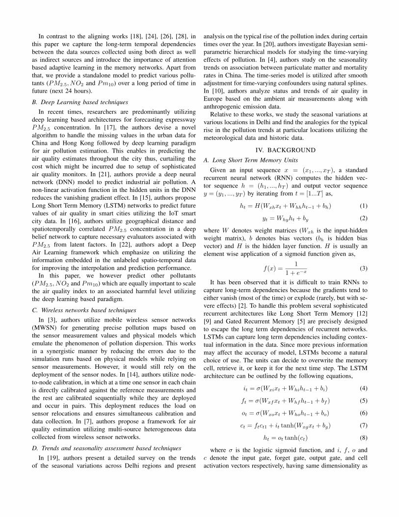
Fig. 2: Unfolded architecture of BiLSTM with 3 consecutivesteps. xt−1, xt, xt+1 represent the inputs to the BiLSTM stepsand yt−1, yt, yt+1 represent the outputs of the BiLSTM steps.
the hidden vector h. The weight matrices from the cell to gatevectors denoted by Wxi are diagonal, so element m in eachgate vector only receives input from element m of the cellvector.
B. Bidirectional LSTM UnitBidirectional LSTM (BiLSTM) [8] utilizes two LSTMs to
process sequence in two directions: forward and backward asshown in Fig. 2. The forward layer output sequence
−→h , is
iteratively calculated using inputs in a positive sequence fromtime T − 1 to time T + 1, while the backward layer outputsequence
←−h , is calculated using the reversed inputs from time
T + 1 to time T − 1. Both the forward and backward layeroutputs are calculated by using the standard LSTM eqns. 4 -9.
BiLSTM generates an output vector Yt, in which eachelement is calculated as follows,
yt = σ(−→h ,←−h ) (9)
where σ function is used to combine the two output sequences.It can be a concatenating function, a summation function,an average function or a multiplication function. Similar tothe LSTM layer, the final output of a BiLSTM layer can berepresented by a vector, Yt = [Yt−n, ....yt−1] in which the lastelement yt−1, is the predicted air pollution prediction for thenext time iteration.
C. Attention mechanismAttentive neural networks have recently demonstrated suc-
cess in a wide range of tasks ranging from question answering[11], machine translations [27] to speech recognition [6]. Inthis section, we propose the attention mechanism for pollu-tion forecasting tasks which assesses the importance of therepresentations of the encoding information ei and computesa weighted sum:
cj =1
E
E∑i=1
wjiei (10)
HISTORICAL DATA
FEATURE EXTRACTION MODEL EVALUATIONPREDICTIONS
PREDICTIONSSTREAM DATA MODELCLOUD STORAGE
OFFLINE TRAINING
ONLINE INFERENCE
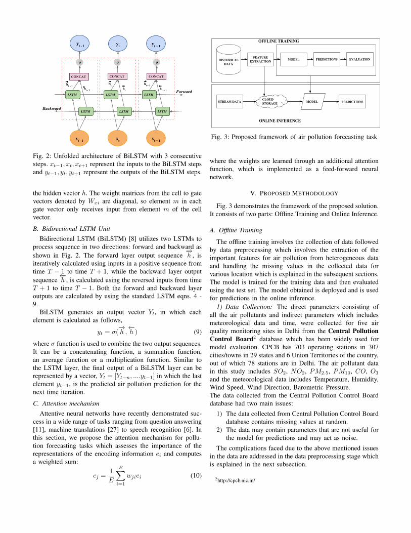
Fig. 3: Proposed framework of air pollution forecasting task
where the weights are learned through an additional attentionfunction, which is implemented as a feed-forward neuralnetwork.
V. PROPOSED METHODOLOGY
Fig. 3 demonstrates the framework of the proposed solution.It consists of two parts: Offline Training and Online Inference.
A. Offline Training
The offline training involves the collection of data followedby data preprocessing which involves the extraction of theimportant features for air pollution from heterogeneous dataand handling the missing values in the collected data forvarious location which is explained in the subsequent sections.The model is trained for the training data and then evaluatedusing the test set. The model obtained is deployed and is usedfor predictions in the online inference.
1) Data Collection: The direct parameters consisting ofall the air pollutants and indirect parameters which includesmeteorological data and time, were collected for five airquality monitoring sites in Delhi from the Central PollutionControl Board2 database which has been widely used formodel evaluation. CPCB has 703 operating stations in 307cities/towns in 29 states and 6 Union Territories of the country,out of which 78 stations are in Delhi. The air pollutant datain this study includes SO2, NO2, PM2.5, PM10, CO, O3
and the meteorological data includes Temperature, Humidity,Wind Speed, Wind Direction, Barometric Pressure.The data collected from the Central Pollution Control Boarddatabase had two main issues:
1) The data collected from Central Pollution Control Boarddatabase contains missing values at random.
2) The data may contain parameters that are not useful forthe model for predictions and may act as noise.
The complications faced due to the above mentioned issuesin the data are addressed in the data preprocessing stage whichis explained in the next subsection.
2http://cpcb.nic.in/
XT - n XT - (n-1) XT - 2 XT - 1 .....
Bi-LSTM Bi-LSTM Bi-LSTMBi-LSTM……...
Attention AttentionAttention Attention……...
Spatial time series inputs (direct and indirect parameters)
Learning Spatial- Temporal features
Further learning using Bi-LSTM (optional)
Prediction resultsXT +2 XT + 1XT + a …..
LSTM
LSTM
σ
CONCAT
LSTM
LSTM
σ
CONCAT
LSTM
LSTM
σ
CONCAT
LSTM
LSTM
σ
CONCAT
……..
σ
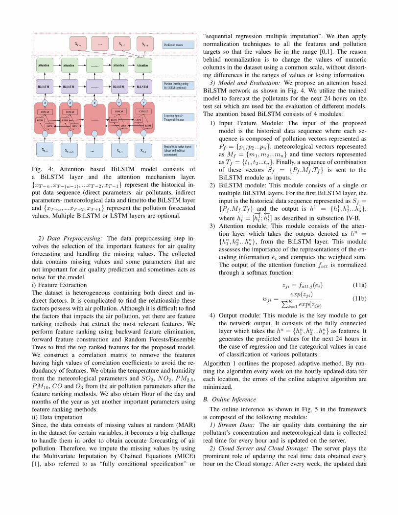
Fig. 4: Attention based BiLSTM model consists ofa BiLSTM layer and the attention mechanism layer.{xT−n, xT−(n−1), ...xT−2, xT−1} represent the historical in-put data sequence (direct parameters- air pollutants, indirectparameters- meteorological data and time)to the BiLSTM layerand {xT+a, ...xT+2, xT+1} represent the pollution forecastedvalues. Multiple BiLSTM or LSTM layers are optional.
2) Data Preprocessing: The data preprocessing step in-volves the selection of the important features for air qualityforecasting and handling the missing values. The collecteddata contains missing values and some parameters that arenot important for air quality prediction and sometimes acts asnoise for the model.i) Feature ExtractionThe dataset is heterogeneous containing both direct and in-direct factors. It is complicated to find the relationship thesefactors possess with air pollution. Although it is difficult to findthe factors that impacts the air pollution, yet there are featureranking methods that extract the most relevant features. Weperform feature ranking using backward feature elimination,forward feature construction and Random Forests/EnsembleTrees to find the top ranked features for the proposed model.We construct a correlation matrix to remove the featureshaving high values of correlation coefficients to avoid the re-dundancy of features. We obtain the temperature and humidityfrom the meteorological parameters and SO2, NO2, PM2.5,PM10, CO and O3 from the air pollution parameters after thefeature ranking methods. We also obtain Hour of the day andmonths of the year as yet another important parameters usingfeature ranking methods.ii) Data imputationSince, the data consists of missing values at random (MAR)in the dataset for certain variables, it becomes a big challengeto handle them in order to obtain accurate forecasting of airpollution. Therefore, we impute the missing values by usingthe Multivariate Imputation by Chained Equations (MICE)[1], also referred to as “fully conditional specification” or
“sequential regression multiple imputation”. We then applynormalization techniques to all the features and pollutiontargets so that the values lie in the range [0,1]. The reasonbehind normalization is to change the values of numericcolumns in the dataset using a common scale, without distort-ing differences in the ranges of values or losing information.
3) Model and Evaluation: We propose an attention basedBiLSTM network as shown in Fig. 4. We utilize the trainedmodel to forecast the pollutants for the next 24 hours on thetest set which are used for the evaluation of different models.The attention based BiLSTM consists of 4 modules:
1) Input Feature Module: The input of the proposedmodel is the historical data sequence where each se-quence is composed of pollution vectors represented asPf = {p1, p2...pn}, meteorological vectors representedas Mf = {m1,m2...mn} and time vectors representedas Tf = {t1, t2...tn}. Finally, a sequence of combinationof these vectors Sf = {Pf .Mf .Tf} is sent to theBiLSTM module as inputs.
2) BiLSTM module: This module consists of a single ormultiple BiLSTM layers. For the first BiLSTM layer, theinput is the historical data sequence represented as Sf ={Pf .Mf .Tf} and the output is h1 = {h11, h12...h1s},where h1t = [
−→h1t ;←−h1t ] as described in subsection IV-B.
3) Attention module: This module consists of the atten-tion layer which takes the outputs denoted as hn ={hn1 , hn2 ...hns }, from the BiLSTM layer. This moduleassesses the importance of the representations of the en-coding information ei and computes the weighted sum.The output of the attention function fatt is normalizedthrough a softmax function:
zji = fatt,j(ei) (11a)
wji =exp(zji)∑Ek=1 exp(zjk)
(11b)
4) Output module: This module is the key module to getthe network output. It consists of the fully connectedlayer which takes the hn = {hn1 , hn2 ...hns } as features. Itgenerates the predicted values for the next 24 hours inthe case of regression and the categorical values in caseof classification of various pollutants.
Algorithm 1 outlines the proposed adaptive method. By run-ning the algorithm every week on the hourly updated data foreach location, the errors of the online adaptive algorithm areminimized.
B. Online Inference
The online inference as shown in Fig. 5 in the frameworkis composed of the following modules:
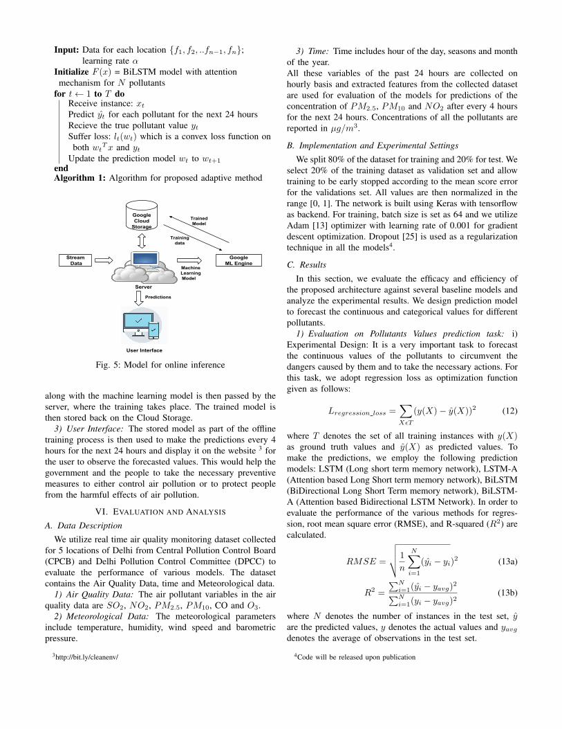
1) Stream Data: The air quality data containing the airpollutant’s concentration and meteorological data is collectedreal time for every hour and is updated on the server.
2) Cloud Server and Cloud Storage: The server plays theprominent role of updating the real time data obtained everyhour on the Cloud storage. After every week, the updated data
Input: Data for each location {f1, f2, ..fn−1, fn};learning rate α
Initialize F (x) = BiLSTM model with attentionmechanism for N pollutants
for t← 1 to T doReceive instance: xtPredict yt for each pollutant for the next 24 hoursRecieve the true pollutant value ytSuffer loss: lt(wt) which is a convex loss function on
both wtTx and ytUpdate the prediction model wt to wt+1
endAlgorithm 1: Algorithm for proposed adaptive method
Google Cloud
Storage
Stream Data
Server
User Interface
Google ML Engine
Machine Learning
Model
Predictions
Training data
Trained Model
Fig. 5: Model for online inference
along with the machine learning model is then passed by theserver, where the training takes place. The trained model isthen stored back on the Cloud Storage.
3) User Interface: The stored model as part of the offlinetraining process is then used to make the predictions every 4hours for the next 24 hours and display it on the website 3 forthe user to observe the forecasted values. This would help thegovernment and the people to take the necessary preventivemeasures to either control air pollution or to protect peoplefrom the harmful effects of air pollution.
VI. EVALUATION AND ANALYSIS
A. Data Description
We utilize real time air quality monitoring dataset collectedfor 5 locations of Delhi from Central Pollution Control Board(CPCB) and Delhi Pollution Control Committee (DPCC) toevaluate the performance of various models. The datasetcontains the Air Quality Data, time and Meteorological data.
1) Air Quality Data: The air pollutant variables in the airquality data are SO2, NO2, PM2.5, PM10, CO and O3.
2) Meteorological Data: The meteorological parametersinclude temperature, humidity, wind speed and barometricpressure.
3http://bit.ly/cleanenv/
3) Time: Time includes hour of the day, seasons and monthof the year.All these variables of the past 24 hours are collected onhourly basis and extracted features from the collected datasetare used for evaluation of the models for predictions of theconcentration of PM2.5, PM10 and NO2 after every 4 hoursfor the next 24 hours. Concentrations of all the pollutants arereported in µg/m3.
B. Implementation and Experimental Settings
We split 80% of the dataset for training and 20% for test. Weselect 20% of the training dataset as validation set and allowtraining to be early stopped according to the mean score errorfor the validations set. All values are then normalized in therange [0, 1]. The network is built using Keras with tensorflowas backend. For training, batch size is set as 64 and we utilizeAdam [13] optimizer with learning rate of 0.001 for gradientdescent optimization. Dropout [25] is used as a regularizationtechnique in all the models4.
C. Results
In this section, we evaluate the efficacy and efficiency ofthe proposed architecture against several baseline models andanalyze the experimental results. We design prediction modelto forecast the continuous and categorical values for differentpollutants.
1) Evaluation on Pollutants Values prediction task: i)Experimental Design: It is a very important task to forecastthe continuous values of the pollutants to circumvent thedangers caused by them and to take the necessary actions. Forthis task, we adopt regression loss as optimization functiongiven as follows:
Lregression loss =∑XεT
(y(X)− y(X))2 (12)
where T denotes the set of all training instances with y(X)as ground truth values and y(X) as predicted values. Tomake the predictions, we employ the following predictionmodels: LSTM (Long short term memory network), LSTM-A(Attention based Long Short term memory network), BiLSTM(BiDirectional Long Short Term memory network), BiLSTM-A (Attention based Bidirectional LSTM Network). In order toevaluate the performance of the various methods for regres-sion, root mean square error (RMSE), and R-squared (R2) arecalculated.
RMSE =
√√√√ 1
n
N∑i=1
(yi − yi)2 (13a)
R2 =
∑Ni=1(yi − yavg)2∑Ni=1(yi − yavg)2
(13b)
where N denotes the number of instances in the test set, yare the predicted values, y denotes the actual values and yavgdenotes the average of observations in the test set.
4Code will be released upon publication
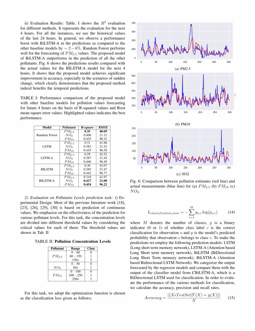
ii) Evaluation Results: Table. I shows the R2 evaluationfor different methods. It represents the evaluation for the next4 hours. For all the instances, we use the historical valuesof the last 24 hours. In general, we observe a performanceboost with BiLSTM-A in the predictions as compared to theother baseline models by ∼ 2− 6%. Random Forest performswell for the forecasting of PM2.5 values. The proposed modelof BiLSTM-A outperforms in the prediction of all the otherpollutants. Fig. 6 shows the predictions results compared withthe actual values for the BILSTM-A model for the next 4hours. It shows that the proposed model achieves significantimprovement in accuracy, especially in the scenarios of suddenchange, which clearly demonstrates that the proposed methodindeed benefits the temporal predictions.
TABLE I: Performance comparison of the proposed modelwith other baseline models for pollution values forecastingfor future 4 hours on the basis of R-squared values and Rootmean square error values. Highlighted values indicates the bestperformance.
Model Pollutants R-square RMSEPM2.5 0.35 40.69
Random Forest NO2 0.406 21.12PM10 0.425 98.32PM2.5 0.31 41.96
LSTM NO2 0.383 21.52PM10 0.445 96.58PM2.5 0.29 42.52
LSTM-A NO2 0.387 21.44PM10 0.446 96.49PM2.5 0.30 42.07
BILSTM NO2 0.385 21.47PM10 0.442 96.77PM2.5 0.310 41.97
BILSTM-A NO2 0.417 21.08PM10 0.454 96.22
2) Evaluation on Pollutants Levels prediction task: i) Ex-perimental Design: Most of the previous literature work [18],[23], [26], [29], [30] is based on prediction of continuousvalues. We emphasize on the effectiveness of the prediction forvarious pollutant levels. For this task, the concentration levelsare divided into different threshold values by considering thecritical values for each of them. The threshold values areshown in Tab. II
TABLE II: Pollution Concentration Levels
Pollutant Range Class0 - 60 0
PM2.5 60 - 150 1150+ 20 - 50 0
NO2 50+ 10 - 100 0
PM10 100 - 250 1250+ 2
For this task, we adopt the optimization function is chosenas the classification loss given as follows:
(a) PM2.5
(b) PM10
(c) NO2
Fig. 6: Comparison between pollution estimates (red line) andactual measurements (blue line) for (a) PM2.5 (b) PM10 (c)NO2.
Lclassification loss = −M∑c=1
yo,c log(po,c) (14)
where M denotes the number of classes, y is a binaryindicator (0 or 1) of whether class label c is the correctclassification for observation o and p is the model’s predictedprobability that observation o belongs to class c. To make thepredictions we employ the following prediction models: LSTM(Long short term memory network), LSTM-A (Attention basedLong Short term memory network), BiLSTM (BiDirectionalLong Short Term memory network), BiLSTM-A (Attentionbased Bidirectional LSTM Network). We categorize the outputforecasted by the regressor models and compare them with theoutput of the classifier model from CBiLSTM-A, which is aBiDirectional LSTM used for classification. In order to evalu-ate the performance of the various methods for classification,we calculate the accuracy, precision and recall rates.
Accuracy =|{XεTestSet|Y (X) = y(X)}|
N(15)
where N is the number of instances in the test set, Y arethe predicted values and y are the actual values.
Precision =true positives
true positives+ false negatives(16)
Precision is defined as the number of true positives dividedby the number of true positives plus the number of falsepositives. False positives are cases the model incorrectlylabels as positive that are actually negative, or in our example,individuals the model classifies as terrorists that are not.
Recall =true positives
true positives+ false positives(17)
Recall is the number of true positives divided by the number oftrue positives plus the number of false negatives. True positivesare data point classified as positive by the model that actuallyare positive (meaning they are correct), and false negatives aredata points the model identifies as negative that actually arepositive (incorrect).ii) Evaluation Results: Table III shows the evaluation of pollu-tion level forecasting by comparing accuracy, precision, recalland F1 Score of all the models. It represents the evaluationfor the next 4 hours. For all the instances for the classificationtask we use the historical values of last 24 hours.
TABLE III: Performance comparison of the proposed modelwith other baseline models for pollution levels forecasting forfuture 4 hours on the basis of Accuracy, average precision andaverage recall. Higher values of accuracy, precision and recallindicates the better performance of the model. Highlightedvalues indicates the best performance.
Model Pollutants Accuracy Precision RecallPM2.5 67.68 56.15 52.27
LSTM NO2 76.85 76.29 75.2PM10 68.34 71.11 56.31PM2.5 67.24 56.46 52.56
LSTM-A NO2 76.85 76.15 75.65PM10 68.71 70.21 57.89PM2.5 67.96 58.35 53.12
BILSTM NO2 77.32 76.75 75.86PM10 68.87 70.25 58.36PM2.5 67.96 55.71 52.55
BILSTM-A NO2 77.66 77.1 76.26PM10 68.21 69.21 57.73PM2.5 70.68 61.06 55.8
CBILSTM-A NO2 77.88 77.56 76.14PM10 67.45 68.23 58.52
It shows that BiLSTM-A shows slight in accuracy comparedto the other models used in the air pollution prediction task.BiLSTM with attention (BiLSTM-A) is preferred over BiL-STM because when Attention mechanism is applied on top ofBiLSTM, it captures periods and makes BiLSTM more robustto random missing values.
D. Trends in Pollution
Delhi is located at 28.61°N 77.23°E, and lies in NorthernIndia. The area represents high seasonal variation. Delhi iscovered by the Great Indian desert (Thar desert) of Rajasthan
on its west and central hot plains in its south part. Thenorth and east boundaries are covered with cool hilly regions.Thus, Delhi is located in the subtropical belt with extremelyscorching summers, moderate rainfall, and chilling winters.
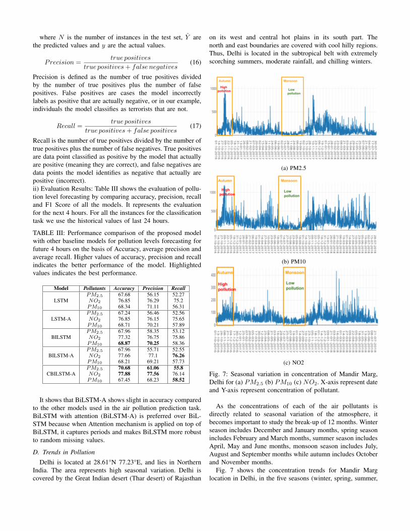
(a) PM2.5
(b) PM10
(c) NO2
Fig. 7: Seasonal variation in concentration of Mandir Marg,Delhi for (a) PM2.5 (b) PM10 (c) NO2. X-axis represent dateand Y-axis represent concentration of pollutant.
As the concentrations of each of the air pollutants isdirectly related to seasonal variation of the atmosphere, itbecomes important to study the break-up of 12 months. Winterseason includes December and January months, spring seasonincludes February and March months, summer season includesApril, May and June months, monsoon season includes July,August and September months while autumn includes Octoberand November months.
Fig. 7 shows the concentration trends for Mandir Marglocation in Delhi, in the five seasons (winter, spring, summer,
monsoon and autumn), from October 2016 to July 2018. Theconcentration of Mandir Marg area was comparatively worstin winter and best in monsoon. The following sequence in thedecreasing order was observed in the concentration of PM10,PM2.5 and NO2: winter > autumn > spring > summer >monsoon. Decreasing order of concentration implies air qualitygoing from worst to better, it means here that winter has worstair quality and monsoon has best.
High concentration is observed after 4pm due to vehicularemission. The concentration of NO2 is highest during 8 am- 10:30 am and 4 pm - 7 pm due to the vehicular emission,from the burning of fuel, from emissions from cars, trucks,buses etc.
E. Real Time Learning System
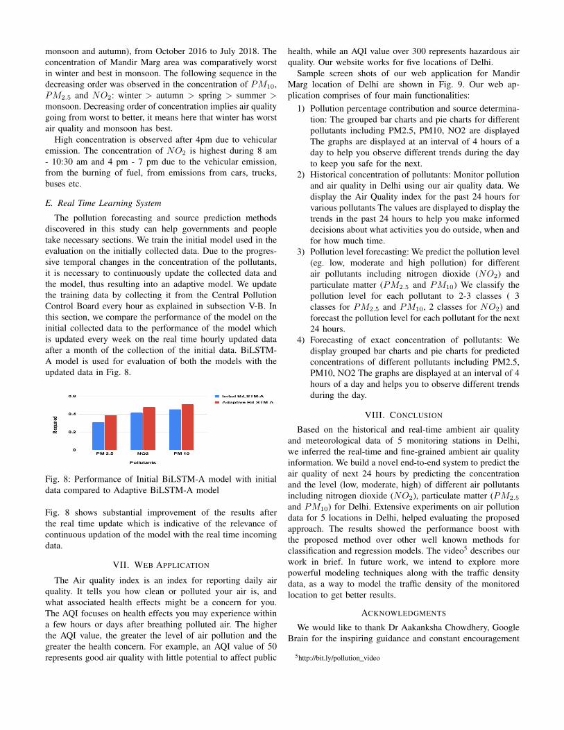
The pollution forecasting and source prediction methodsdiscovered in this study can help governments and peopletake necessary sections. We train the initial model used in theevaluation on the initially collected data. Due to the progres-sive temporal changes in the concentration of the pollutants,it is necessary to continuously update the collected data andthe model, thus resulting into an adaptive model. We updatethe training data by collecting it from the Central PollutionControl Board every hour as explained in subsection V-B. Inthis section, we compare the performance of the model on theinitial collected data to the performance of the model whichis updated every week on the real time hourly updated dataafter a month of the collection of the initial data. BiLSTM-A model is used for evaluation of both the models with theupdated data in Fig. 8.
Fig. 8: Performance of Initial BiLSTM-A model with initialdata compared to Adaptive BiLSTM-A model
Fig. 8 shows substantial improvement of the results afterthe real time update which is indicative of the relevance ofcontinuous updation of the model with the real time incomingdata.
VII. WEB APPLICATION
The Air quality index is an index for reporting daily airquality. It tells you how clean or polluted your air is, andwhat associated health effects might be a concern for you.The AQI focuses on health effects you may experience withina few hours or days after breathing polluted air. The higherthe AQI value, the greater the level of air pollution and thegreater the health concern. For example, an AQI value of 50represents good air quality with little potential to affect public
health, while an AQI value over 300 represents hazardous airquality. Our website works for five locations of Delhi.
Sample screen shots of our web application for MandirMarg location of Delhi are shown in Fig. 9. Our web ap-plication comprises of four main functionalities:
1) Pollution percentage contribution and source determina-tion: The grouped bar charts and pie charts for differentpollutants including PM2.5, PM10, NO2 are displayedThe graphs are displayed at an interval of 4 hours of aday to help you observe different trends during the dayto keep you safe for the next.
2) Historical concentration of pollutants: Monitor pollutionand air quality in Delhi using our air quality data. Wedisplay the Air Quality index for the past 24 hours forvarious pollutants The values are displayed to display thetrends in the past 24 hours to help you make informeddecisions about what activities you do outside, when andfor how much time.
3) Pollution level forecasting: We predict the pollution level(eg. low, moderate and high pollution) for differentair pollutants including nitrogen dioxide (NO2) andparticulate matter (PM2.5 and PM10) We classify thepollution level for each pollutant to 2-3 classes ( 3classes for PM2.5 and PM10, 2 classes for NO2) andforecast the pollution level for each pollutant for the next24 hours.
4) Forecasting of exact concentration of pollutants: Wedisplay grouped bar charts and pie charts for predictedconcentrations of different pollutants including PM2.5,PM10, NO2 The graphs are displayed at an interval of 4hours of a day and helps you to observe different trendsduring the day.
VIII. CONCLUSION
Based on the historical and real-time ambient air qualityand meteorological data of 5 monitoring stations in Delhi,we inferred the real-time and fine-grained ambient air qualityinformation. We build a novel end-to-end system to predict theair quality of next 24 hours by predicting the concentrationand the level (low, moderate, high) of different air pollutantsincluding nitrogen dioxide (NO2), particulate matter (PM2.5
and PM10) for Delhi. Extensive experiments on air pollutiondata for 5 locations in Delhi, helped evaluating the proposedapproach. The results showed the performance boost withthe proposed method over other well known methods forclassification and regression models. The video5 describes ourwork in brief. In future work, we intend to explore morepowerful modeling techniques along with the traffic densitydata, as a way to model the traffic density of the monitoredlocation to get better results.
ACKNOWLEDGMENTS
We would like to thank Dr Aakanksha Chowdhery, GoogleBrain for the inspiring guidance and constant encouragement
5http://bit.ly/pollution video
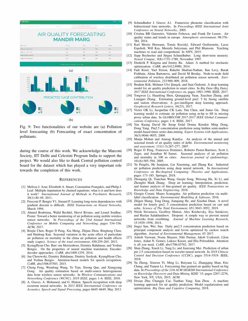
(a)
(b)
Fig. 9: Two functionalities of our website are (a) Pollutionlevel forecasting (b) Forecasting of exact concentration ofpollutants.
during the course of this work. We acknowledge the MarconiSociety, IIT Delhi and Celestini Program India to support theproject. We would also like to thank Central pollution controlboard for the dataset which has played a very important roletowards the completion of this work.
REFERENCES
[1] Melissa J. Azur, Elizabeth A. Stuart, Constantine Frangakis, and Philip J.Leaf. Multiple imputation by chained equations: what is it and how doesit work? International Journal of Methods in Psychiatric Research,20(1):40–49, 2011.
[2] Frasconi P. Bengio Y1, Simard P. Learning long-term dependencies withgradient descent is difficult. IEEE Transactions on Neural Networks,March 1994.
[3] Ahmed Boubrima, Walid Bechkit, Herve Rivano, and Lionel Soulhac.Poster: Toward a better monitoring of air pollution using mobile wirelesssensor networks. In Proceedings of the 23rd Annual InternationalConference on Mobile Computing and Networking, pages 534–536.ACM, 2017.
[4] Renjie Chen, Roger D Peng, Xia Meng, Zhijun Zhou, Bingheng Chen,and Haidong Kan. Seasonal variation in the acute effect of particulateair pollution on mortality in the china air pollution and health effectsstudy (capes). Science of the total environment, 450:259–265, 2013.
[5] KyungHyun Cho, Bart van Merrienboer, Dzmitry Bahdanau, and YoshuaBengio. On the properties of neural machine translation: Encoder-decoder approaches. CoRR, abs/1409.1259, 2014.
[6] Jan Chorowski, Dzmitry Bahdanau, Dmitriy Serdyuk, KyungHyun Cho,and Yoshua Bengio. Attention-based models for speech recognition.CoRR, abs/1506.07503, 2015.
[7] Cheng Feng, Wendong Wang, Ye Tian, Xirong Que, and XiangyangGong. Air quality estimation based on multi-source heterogeneousdata from wireless sensor networks. In Wireless Communications andNetworking Conference (WCNC), 2018 IEEE, pages 1–6. IEEE, 2018.
[8] A. Graves, A. Mohamed, and G. Hinton. Speech recognition with deeprecurrent neural networks. In 2013 IEEE International Conference onAcoustics, Speech and Signal Processing, pages 6645–6649, May 2013.
[9] Schmidhuber J. Graves A1. Framewise phoneme classification withbidirectional lstm networks. In Proceedings IEEE International JointConference on Neural Networks,, 2005.
[10] Cristina BB Guerreiro, Valentin Foltescu, and Frank De Leeuw. Airquality status and trends in europe. Atmospheric environment, 98:376–384, 2014.
[11] Karl Moritz Hermann, Tomas Kocisky, Edward Grefenstette, LasseEspeholt, Will Kay, Mustafa Suleyman, and Phil Blunsom. Teachingmachines to read and comprehend. In NIPS, 2015.
[12] Sepp Hochreiter and Jurgen Schmidhuber. Long short-term memory.Neural Comput., 9(8):1735–1780, November 1997.
[13] Diederik P. Kingma and Jimmy Ba. Adam: A method for stochasticoptimization. CoRR, abs/1412.6980, 2014.
[14] Fadi Kizel, Yael Etzion, Rakefet Shafran-Nathan, Ilan Levy, BarakFishbain, Alena Bartonova, and David M Broday. Node-to-node fieldcalibration of wireless distributed air pollution sensor network. Envi-ronmental Pollution, 233:900–909, 2018.
[15] Ibrahim Kok, Mehmet Ulvi Simsek, and Suat Ozdemir. A deep learningmodel for air quality prediction in smart cities. In Big Data (Big Data),2017 IEEE International Conference on, pages 1983–1990. IEEE, 2017.
[16] Tongwen Li, Huanfeng Shen, Qiangqiang Yuan, Xuechen Zhang, andLiangpei Zhang. Estimating ground-level pm2. 5 by fusing satelliteand station observations: A geo-intelligent deep learning approach.Geophysical Research Letters, 44(23), 2017.
[17] Victor OK Li, Jacqueline CK Lam, Yun Chen, and Jiatao Gu. Deeplearning model to estimate air pollution using m-bp to fill in missingproxy urban data. In GLOBECOM 2017-2017 IEEE Global Communi-cations Conference, pages 1–6. IEEE, 2017.
[18] Yan Kuang David He Serap Erdal Donna Kenskie Ming Dong,Dong Yang. Pm2.5 concentration prediction using hidden semi-markovmodel-based times series data mining. Expert Systems with Applications,36(5):9046–9055, 2009.
[19] Manju Mohan and Anurag Kandya. An analysis of the annual andseasonal trends of air quality index of delhi. Environmental monitoringand assessment, 131(1-3):267–277, 2007.
[20] Roger D Peng, Francesca Dominici, Roberto Pastor-Barriuso, Scott LZeger, and Jonathan M Samet. Seasonal analyses of air pollutionand mortality in 100 us cities. American journal of epidemiology,161(6):585–594, 2005.
[21] Yu Pengfei, He Juanjuan, Liu Xiaoming, and Zhang Kai. Industrialair pollution prediction using deep neural network. In InternationalConference on Bio-Inspired Computing: Theories and Applications,pages 173–185. Springer, 2018.
[22] Zhongang Qi, Tianchun Wang, Guojie Song, Weisong Hu, Xi Li, andZhongfei Mark Zhang. Deep air learning: Interpolation, prediction,and feature analysis of fine-grained air quality. IEEE Transactions onKnowledge and Data Engineering, 2018.
[23] Giorgio Corani; Mauro Scanagatta. Air pollution prediction via multi-label classification. Environmental Modelling & Software, 2016.
[24] Zhigen Shang, Tong Deng, Jianqiang He, and Xiaohui Duan. A novelmodel for hourly pm2. 5 concentration prediction based on cart andeelm. Science of The Total Environment, 651:3043–3052, 2019.
[25] Nitish Srivastava, Geoffrey Hinton, Alex Krizhevsky, Ilya Sutskever,and Ruslan Salakhutdinov. Dropout: A simple way to prevent neuralnetworks from overfitting. Journal of Machine Learning Research,15:1929–1958, 2014.
[26] Jingyi Sun, Wei; Sun. Daily pm2.5 concentration prediction based onprincipal component analysis and lssvm optimized by cuckoo searchalgorithm. Journal of Environmental Management, 03 2017.
[27] Ashish Vaswani, Noam Shazeer, Niki Parmar, Jakob Uszkoreit, LlionJones, Aidan N. Gomez, Lukasz Kaiser, and Illia Polosukhin. Attentionis all you need. CoRR, abs/1706.03762, 2017.
[28] Shan Zhang, Xiaoli Li, Yang Li, and Jianxiang Mei. Prediction of urbanpm 2.5 concentration based on wavelet neural network. In 2018 ChineseControl And Decision Conference (CCDC), pages 5514–5519. IEEE,2018.
[29] Yu Zheng, Xiuwen Yi, Ming Li, Ruiyuan Li, Zhangqing Shan, EricChang, and Tianrui Li. Forecasting fine-grained air quality based on bigdata. In Proceedings of the 21th ACM SIGKDD International Conferenceon Knowledge Discovery and Data Mining, KDD ’15, pages 2267–2276,New York, NY, USA, 2015. ACM.
[30] Dixian Zhu; Changjie Cai; Tianbao Yang; Xun Zhou. A machinelearning approach for air quality prediction: Model regularization andoptimization. Big Data and Cognitive Computing, 2018.