1

U S C L I V A R V A R I A T I O N S

US CLIVAR VARIATIONS • Spring 2017 • Vol. 15, No. 2 1

IN THIS ISSUE

Roles of the deep ocean in climate

Gregory C. Johnson*,1 and Michael Winton2

1NOAA Pacific Marine Environmental Laboratory2NOAA Geophysical Fluid Dynamics Laboratory

VARIATIONS Spring 2017 • Vol. 15, No. 2

US CLIVARClimate Variability & Predictabilit

y

Roles of the deep ocean in climate......................................................................................................... 1

Global Ocean Ship-based Hydrographic Investigations Program (GO-SHIP) provides key climate-relevant

deep ocean observations ........................................................................................................................ 8

Deep moored observations and OceanSITES ...................................................................................... 15

Remote sensing of bottom pressure from GRACE satellites................................................................. 22

The Argo program samples the deep ocean ......................................................................................... 29

Deepgliders for observing ocean circulation and climate ...................................................................... 34

A case for observing the deep ocean

Guest Editor: Renellys Perez

U. Miami/NOAA AOML

The past few decades have seen an unprecedented increase in the number of physical and biogeochemical measurements in the global oceans. These observations are crucial for documenting how the ocean interacts with the overlying atmosphere. We know that ocean variations have profound effects on weather and climate and can strongly influence surrounding coastlines and coastal communities. Further, the ocean circulates and redistributes heat, salt, carbon, and nutrients around the globe, having major impacts on the systems that sustain marine life and ecosystem diversity. In essence, ocean observations supply information important to society.

To date, the primary focus of the global ocean observing system has been on the surface and intermediate layers of the ocean. Far fewer observations are being collected in the deep layers – here defined as below 2000 m. For example, less than 15% of the holdings in the World Ocean Database are from below 2000 m. This drops to less than 1% below 4000 m. The majority of these deep measurements were obtained from hydrographic surveys, which produce highly accurate data but require substantial personnel and ship time resources.

1

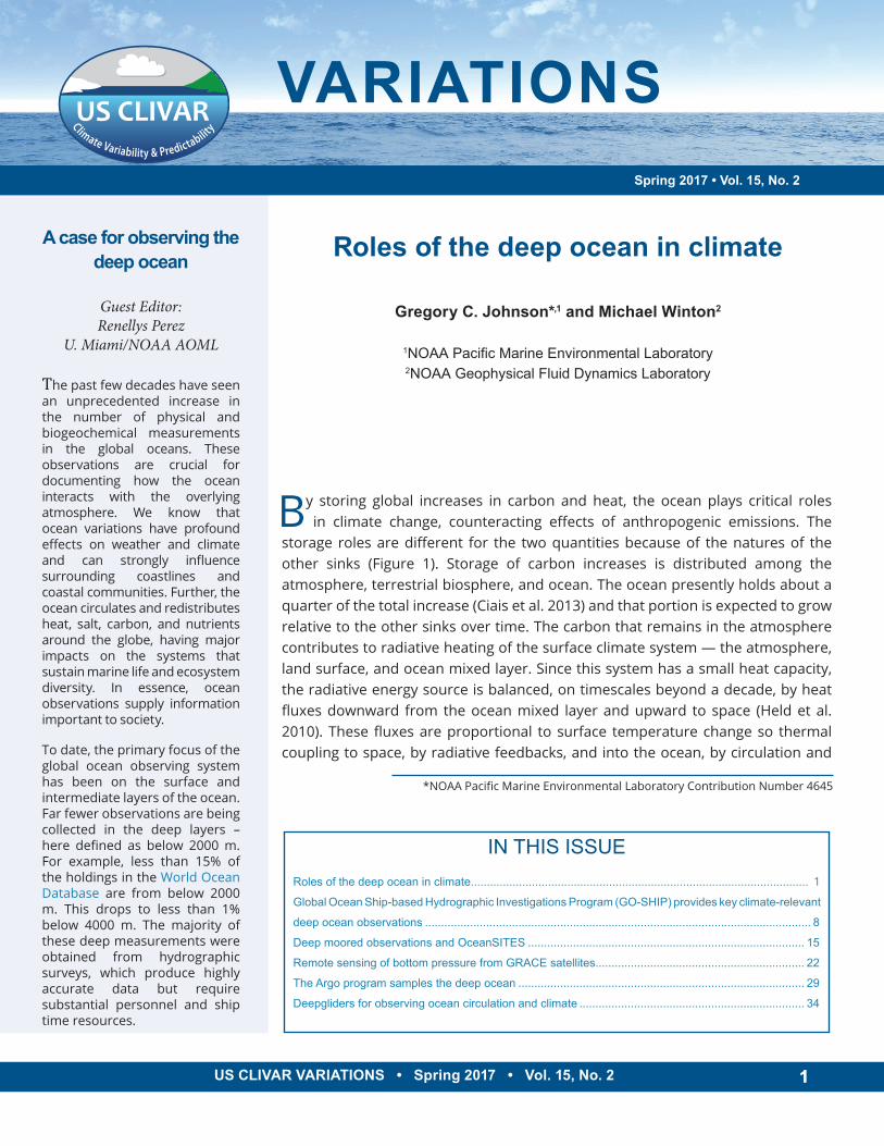
By storing global increases in carbon and heat, the ocean plays critical roles in climate change, counteracting effects of anthropogenic emissions. The

storage roles are different for the two quantities because of the natures of the other sinks (Figure 1). Storage of carbon increases is distributed among the atmosphere, terrestrial biosphere, and ocean. The ocean presently holds about a quarter of the total increase (Ciais et al. 2013) and that portion is expected to grow relative to the other sinks over time. The carbon that remains in the atmosphere contributes to radiative heating of the surface climate system — the atmosphere, land surface, and ocean mixed layer. Since this system has a small heat capacity, the radiative energy source is balanced, on timescales beyond a decade, by heat fluxes downward from the ocean mixed layer and upward to space (Held et al. 2010). These fluxes are proportional to surface temperature change so thermal coupling to space, by radiative feedbacks, and into the ocean, by circulation and

*NOAA Pacific Marine Environmental Laboratory Contribution Number 4645

2

We know that the deep ocean plays a crucial role in the Earth’s climate, primarily through property redistribution via the large-scale overturning circulation, as well as serving as a massive reservoir for heat and carbon storage. Although the deep ocean has long been perceived to be slowly changing, the limited observations from the last few decades show pronounced changes in deep water mass properties. These changes suggest that the deep ocean has already begun storing excess heat and carbon from the atmosphere and is, thus, playing an important role in the Earth’s energy imbalance and carbon cycle.

Expanding the global ocean observation system into the deep ocean is in the best interest of humanity. The main obstacles to enhancing the deep ocean observing system include limited ship time, inadequate funding, and the technical challenges posed by collecting high-quality measurements in an extreme environment. This edition of Variations highlights the existing “state-of-the-art” methods to measure the deep ocean, some of the scientific insights that have already been gained from these observations, and new methodologies and technologies to expand the network of deep observations.

U S CL I VA RVA R I AT I O N S

Editor:Kristan Uhlenbrock

US CLIVAR Project Office1201 New York Ave NW, Suite 400

Washington, DC 20005202-787-1682 | www.usclivar.org

diffusion, jointly determine a surface warming magnitude that balances the radiative forcing. In contrast to its carbon uptake, the ocean has gained over 90% of the global energy imbalance (Rhein et al. 2013). Ocean uptake of carbon and heat mitigate surface warming but contribute impacts of their own through ocean acidification, habitat shifts, and sea level rise.

Consider the response of these balances to an anthropogenic pulse of carbon emitted to the atmosphere as simulated by climate models (Joos et al. 2013). During the emission, the ocean reduces warming of the surface climate system by removing atmospheric carbon, hence reducing the radiative forcing, and by taking up heat at an increasing rate. After emission, the offsetting effect of ocean carbon uptake continues for millennia until the ocean and atmosphere strike a new chemical balance, with the ocean containing most of the emitted carbon. Ocean heat uptake diminishes over this period as deep ocean temperatures approach equilibrium with the declining atmospheric CO2 forcing, a warming effect that opposes the carbon uptake. Models typically show these two effects balancing, leading to relatively stable warming over the post-emission period, although

Figure 1. Schematic balances for carbon and heat. CO2 accumulates significantly in the atmosphere, the land, and, increasingly, the ocean. Heat is lost to space and accumulates in the ocean.

.

CO2 Heat

.. .... . . . .... . . .. .

dominantpost-emissionbalances

3

U S C L I V A R V A R I A T I O N S

US CLIVAR VARIATIONS • Spring 2017 • Vol. 15, No. 2 3

there is a considerable range of simulated post-emission trends (Frölicher et al. 2014). Although the role of the processes described above is conceptually clearest in the post-carbon-emission period, they also contribute to the present-day response to anthropogenic emissions.

The balances that determine long-term climate evolution are effected by ocean circulation and diffusion distributing heat and carbon increases, stemming from anthropogenic emissions, throughout the ocean. Hence, deep and bottom water formation over centennial to millennial timescales is important for the long-term evolution of the warming. As discussed below, model simulations of present-day deep and bottom water formation and their response to changing climate differ greatly and suffer from well-known biases, calling into question their fidelity on long timescales. Consequently, observation and monitoring of deep and bottom water formation, properties, and circulation are crucial for constraining climate models and their projections.

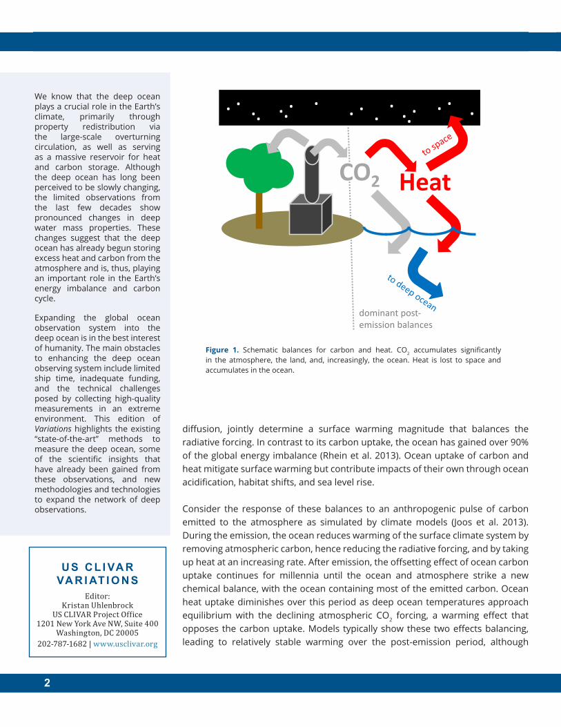
The two major water-masses filling the deep ocean (Figure 2) are Antarctic Bottom Water (AABW), and North Atlantic Deep Water (NADW). AABW originates as a result of complex ocean-ice-atmosphere interactions around the margins of Antarctica, with plumes of very cold, dense waters formed on the continental shelves descending the continental slopes to the abyssal ocean, entraining offshore ambient waters by turbulent mixing as they do so

(Orsi et al. 1999). NADW is formed from a mixture of open-ocean convection to mid-depths in the Labrador Sea and turbulent plumes of dense overflows located between Greenland and the Shetland Islands (Yashayaev 2007). Together, AABW and NADW account for over half of the water-mass volume in the ocean, with the AABW volume estimated at 36% of the total, and NADW at 21% (Johnson 2008). Zonally averaged around the globe, AABW concentrations peak in the Southern Ocean and the abyss, whereas NADW has its highest concentrations in the North Atlantic Ocean, and at mid-depth.

Figure 2. Vertical meridional sections of fractional concentrations of North Atlantic Deep Water (NADW; top panels) and Antarctic Bottom Water (AABW; bottom panels) zonally averaged across the Indo-Pacific (left panels) and Atlantic (right panels) oeans, based on Johnson (2008). Concentrations are contoured at 0.1 intervals from < 0.1 (white) to > 0.9 (darkest blue). Select neutral isopycnals (thick black lines) are contoured, 28.03 and 27.6 kg m-3 in the Indo-Pacific and 28.11  and 27.7 kg m-3 in the Atlantic, as the approximate divisions (e.g., Lumpkin and Speer 2007) between northward flowing bottom waters, southward flowing deep waters, and the intermediate waters above them. Latitude is reversed in the Indo-Pacific versus the Atlan-tic, so the Antarctic is toward the center of the figure (negative values), and the Arctic toward its right and left borders (positive values).

4

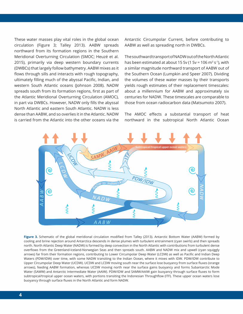
These water masses play vital roles in the global ocean circulation (Figure 3; Talley 2013). AABW spreads northward from its formation regions in the Southern Meridional Overturning Circulation (SMOC; Heuzé et al. 2015), primarily via deep western boundary currents (DWBCs) that largely follow bathymetry. AABW mixes as it flows through sills and interacts with rough topography, ultimately filling much of the abyssal Pacific, Indian, and western South Atlantic oceans (Johnson 2008). NADW spreads south from its formation regions, first as part of the Atlantic Meridional Overturning Circulation (AMOC), in part via DWBCs. However, NADW only fills the abyssal North Atlantic and eastern South Atlantic. NADW is less dense than AABW, and so overlies it in the Atlantic. NADW is carried from the Atlantic into the other oceans via the

Antarctic Circumpolar Current, before contributing to AABW as well as spreading north in DWBCs.

The southward transport of NADW out of the North Atlantic has been estimated at about 15 Sv (1 Sv = 106 m3 s-1), with a similar magnitude northward transport of AABW out of the Southern Ocean (Lumpkin and Speer 2007). Dividing the volumes of these water masses by their transports yields rough estimates of their replacement timescales: about a millennium for AABW and approximately six centuries for NADW. These timescales are comparable to those from ocean radiocarbon data (Matsumoto 2007).

The AMOC effects a substantial transport of heat northward in the subtropical North Atlantic Ocean

A A B W

LC

DW

Subtropical/tropical upper ocean waters

N A D W

PDW/IDW

ITF

SAMW, AAIWUCD

W

NA

DW

AA

BW

NADW to Indian

Figure 3. Schematic of the global meridional circulation modified from Talley (2013). Antarctic Bottom Water (AABW) formed by cooling and brine rejection around Antarctica descends in dense plumes with turbulent entrainment (cyan swirls) and then spreads north. North Atlantic Deep Water (NADW) is formed by deep convection in the North Atlantic with contributions from turbulent dense overflows from the Greenland-Iceland-Norwegian Seas and then spreads south. AABW and NADW mix and upwell (cyan squiggly arrows) far from their formation regions, contributing to Lower Circumpolar Deep Water (LCDW) as well as Pacific and Indian Deep Waters (PDW/IDW) over time, with some NADW transiting to the Indian Ocean, where it mixes with IDW. PDW/IDW contribute to Upper Circumpolar Deep Water (UCDW). UCDW and LCDW moving south near the surface lose buoyancy from surface fluxes (orange arrows), feeding AABW formation, whereas UCDW moving north near the surface gains buoyancy and forms Subantarctic Mode Water (SAMW) and Antarctic Intermediate Water (AAIW). PDW/IDW and SAMW/AAIW gain buoyancy through surface fluxes to form subtropical/tropical upper ocean waters, with portions transiting the Indonesian Throughflow (ITF). These upper ocean waters lose buoyancy through surface fluxes in the North Atlantic and form NADW.

5

U S C L I V A R V A R I A T I O N S

US CLIVAR VARIATIONS • Spring 2017 • Vol. 15, No. 2 5

because of the large temperature contrast between the relatively cold NADW flowing south and the warmer upper ocean waters that flow north (Talley 2003). While the North Atlantic exports carbon southward, it exports less now than in preindustrial times (Macdonald et al. 2003), consistent with a substantial increase in carbon storage in that basin (Woosley et al. 2016). In contrast, the colder, deeper SMOC has a much smaller temperature contrast between AABW flowing north and the very old, but only slightly warmer Circumpolar Deep Water (CDW) flowing south and upwelling in the Antarctic Circumpolar Current, thence feeding both AABW and Antarctic Intermediate Water (AAIW) formation. Thus, the SMOC effects a relatively small heat transport. However, CDW — a mixture of “aged” AABW (including Pacific and Indian Deep Waters), various intermediate and mode waters, and some NADW — has not seen the sea surface for many centuries. Hence, it takes up significant amounts of heat and carbon, relative to preindustrial times, when exposed to the modern atmosphere with its increased carbon concentration and warmth (Russell et al. 2006). Much of this increase in carbon and heat is stored in AAIW as it flows north, with a smaller amount of warming and additional carbon stored in the AABW as it forms.

Variations in deep ocean water properties, including NADW and AABW, reflect surface forcing variations. In the deep Greenland Sea, cessation of ventilation has resulted in warming at a rate similar to the warming rate of Earth’s mean surface temperature over the past several decades (Somavilla et al. 2013). In contrast, formation rates, depths, and water properties of Labrador Sea Water, formed by open-ocean deep convection, have varied decadally, at least in part with fluctuations of the North Atlantic Oscillation (Yashayaev and Loder 2016). Striking warming is found in the AABW over recent decades throughout the Southern Ocean, extending into the abyssal Pacific, western South Atlantic, and eastern Indian1 oceans (Purkey and Johnson 2010; Desbruyères et al. 2016). Furthermore, AABW has been freshening over recent decades, especially in the Indian and Pacific sectors of the Southern Ocean (Purkey and Johnson 2013). Freshening of the Ross Sea Shelf waters, one of the components

of AABW in the region, linked with increased melting of marine terminating ice sheets (Jacobs and Giulivi 2010), may be one factor in observed AABW changes. The increased buoyancy from this freshening may result in a warmer, lighter variety of AABW and reduce the amount of AABW formed. In the Weddell Sea, one hypothesis is that the 1970s Weddell Polynya substantially cooled the deep and abyssal ocean in the region, and the AABW warming observed there may be partly a rebound from that cooling event (de Lavergne et al. 2014).

A frequently asked question is how the warming signal of AABW has already been observed in the North Pacific. The answer is that it has probably not been advected there yet, but is the result of a teleconnection of changing formation (either rates or densities) of AABW by planetary (Kelvin and Rossby) waves (Masuda et al. 2010). This teleconnection effects what oceanographers term an isopycnal “heave” signature of the changes, rather than an advective “water-mass” signature (Bindoff and McDougall 1994). To date, water-mass signatures (changing temperature-salinity relations) in the deep and abyssal ocean are most easily observed near the formation regions of NADW and AABW; although transient gasses such as chlorofluorocarbons, which were introduced into the atmosphere starting in the 1930s and can be observed in the ocean at extremely low concentrations, reveal advective signatures spreading from the formation regions of NADW (LeBel et al. 2008) and AABW (Orsi et al. 2002).

Deep ocean temperature and salinity changes play roles in both the global energy budget and sea level budgets. Ocean warming below 2000 m has been estimated to take up about 10% of Earth’s total energy imbalance during 2005–2015 (Johnson et al. 2016). Deep ocean warming is currently a smaller contributor to global sea level budgets (Purkey and Johnson 2010), since the thermal 1expansion coefficient of seawater is smaller for colder, deeper waters. However, deep ocean temperature and

1The deep western Indian Ocean has not been sampled since the World Ocean Circulation Experiment in 1994 owing to pirate activity.

6

References

Bindoff, N. L., and T. J. McDougall, 1994: Diagnosing climate change and ocean ventilation using hydrographic data. J. Phys. Oceanogr., 24, 1137–1152, doi: 10.1175/1520-0485(1994)024<1137:DCCAOV>2.0.CO;2.

Boé, J., A. Hall, and X. Qu, 2009: Deep ocean heat uptake as a major source of spread in transient climate change simulations. Geophys. Res. Lett., 36, doi:10.1029/2009GL040845.

Carrassi, A., V. Guemas, F. J. Doblas-Reyes, D. Volpi, and M. Asif, 2016: Sources of skill in near-term climate prediction: generating initial conditions. Climate Dyn., 47, 3693–3712, doi:10.1007/s00382-016-3036-4.

Cheng, W., J. C. H. Chiang, and D. X. Zhang, 2013: Atlantic Meridional Overturning Circulation (AMOC) in CMIP5 Models: RCP and historical simulations. J. Climate, 26, 7187–7197, doi:10.1175/JCLI-D-12-00496.1.

salinity variations can contribute substantially to regional sea level variations (Johnson et al. 2008). While deep anthropogenic carbon uptake concentrations are small, they are spread over a large volume and are expected to increase in the future. Furthermore, deep ocean warming has potential to have substantial effects on ecosystems, since historical temperature ranges are small (Levin and Le Bris 2015).

As noted above, predicting future deep ocean changes in a changing climate requires models, and on the flip side, deep ocean conditions can be important in verifying and initializing models. There has been much work in validating climate model ability to simulate the AMOC (Cheng et al. 2013), and analyses of climate impacts of a collapse of the AMOC (Vellinga and Wood 2002). Anti-correlation between preindustrial AMOC strength and global warming relative to equilibrium has been found in climate models (Winton et al. 2014), demonstrating the importance of accurate simulation of deep circulation.

Moreover, standard-resolution climate models generally do not do a good job at forming AABW as observed in the modern ocean (Heuzé et al. 2013), which can lead to unrealistic model deep ocean conditions, which in turn are well correlated with projected rates of warming in climate models (Boé et al. 2009). However, at least one high-resolution climate model forms AABW on the shelf, as observed, and the deep ocean in that model warms about four times faster under CO2 doubling than in the same model at standard resolution (Newsom et al. 2016). Initializing climate models with deep ocean conditions may also improve their estimates of ocean circulation (Carrassi et al. 2016).

Our present observing system of the deep ocean, discussed in the rest of this issue, is fairly sparse, given the importance and influence it has on the climate. GO-SHIP (Talley et al. 2016) collects invaluable, synoptic, coast-to-coast, full-depth, highly accurate, densely sampled (along-track) repeat oceanographic transects of a range of variables including temperature, salinity, velocity, dissolved oxygen and nutrient concentrations, carbon parameters, transient tracers, and more. However, these transects are relatively few and generally only occupied at decadal intervals. Moored measurements such as the RAPID array (McCarthy et al. 2015), which monitors the AMOC at 26.5°N, and OceanSites (Send et al. 2011) deep sensors provide well-resolved time series of and substantial insights into deep ocean variability, but are spatially sparse. Satellite measurements of gravity variations, often combined with satellite sea-surface height variation measurements and temperature and salinity data in the upper 2 km of the ocean from the Argo array, can also illuminate regional deep ocean circulation variability (Landerer et al. 2015). However, uncertainties on global average deep ocean temperature changes inferred from residual calculations using these data are large (Llovel et al. 2014). A global array of Deep Argo floats would greatly reduce these uncertainties (Johnson et al. 2015), complementing GO-SHIP sections, deep mooring measurements, and satellite data by providing large-scale, global, continuous in situ monitoring of varying deep ocean conditions. DeepGliders are another innovative and valuable tool that could increase sampling of the deep ocean along transects or at stations.

7

U S C L I V A R V A R I A T I O N S

US CLIVAR VARIATIONS • Spring 2017 • Vol. 15, No. 2 7

Ciais, P., and Coauthors, 2013: Carbon and Other Biogeochemical Cycles. Climate Change 2013: The Physical Science Basis. Contribution of Working Group I to the Fifth Assessment Report of the Intergovernmental Panel on Climate Change, T. F. Stocker, and Coauthors, Eds., Cambridge University Press, 465–570.

de Lavergne, C., J. B. Palter, E. D. Galbraith, R. Bernardello, and I. Marinov, 2014: Cessation of deep convection in the open Southern Ocean under anthropogenic climate change. Nature Climate Change, 4, 278–282, doi:10.1038/nclimate2132.

Desbruyères, D. G., S. G. Purkey, E. L. McDonagh, G. C. Johnson, and B. A. King, 2016: Deep and abyssal ocean warming from 35 years of repeat hydrography. Geophys. Res. Lett., 43, 10356–10365, doi:10.1002/2016GL070413.

Frölicher, T. L., M. Winton, and J. L. Sarmiento, 2014: Continued global warming after CO2 emissions stoppage. Nature Climate Change, 4, 40–44, doi:10.1038/nclimate2060.

Held, I. M., M. Winton, K. Takahashi, T. Delworth, F. Zeng, and G. K. Vallis, 2010: Probing the fast and slow components of global warming by returning abruptly to preindustrial forcing. J. Climate, 23, 2418–2427, doi:10.1175/2009JCLI3466.1.

Heuzé, C., K. J. Heywood, D. P. Stevens, and J. K. Ridley, 2013: Southern Ocean bottom water characteristics in CMIP5 models. Geophys. Res. Lett., 40, 1409–1414, doi:10.1002/grl.50287.

Jacobs, S. S., and C. F. Giulivi, 2010: Large multidecadal salinity trends near the Pacific–Antarctic continental margin. J. Climate, 23, 4508–4524, doi:10.1175/2010JCLI3284.1.

Johnson, G. C., 2008: Quantifying Antarctic Bottom Water and North Atlantic Deep Water volumes. J. Geophys. Res., 113, doi:10.1029/2007JC004477.

Johnson, G. C., S. G. Purkey, and J. L. Bullister, 2008: Warming and freshening in the abyssal southeastern Indian Ocean. J. Climate, 21, 5351–5363, doi:10.1175/2008JCLI2384.1.

Johnson, G. C., J. M. Lyman, and S. G. Purkey, 2015: Informing Deep Argo array design using Argo and full-depth hydrographic section data. J. Atmos. Ocean. Tech.., 32, 2187–2198, doi:10.1175/JTECH-D-15-0139.1.

Johnson, G. C., J. M. Lyman, and N. G. Loeb, 2016: Correspondence: Improving estimates of Earth's energy imbalance. Nature Climate Change, 6, 639–640, doi:10.1038/nclimate3043.

Joos, F., and Coauthors, 2013: Carbon dioxide and climate impulse response functions for the computation of greenhouse gas metrics: A multi-model analysis. Atmos. Chem. Phys., 13, 2793–2825, doi:10.5194/acp-13-2793-2013.

Landerer, F. W., D. N. Wiese, K. Bentel, C. Boening, and M. M. Watkins, 2015: North Atlantic meridional overturning circulation variations from GRACE ocean bottom pressure anomalies. Geophys. Res. Lett., 42, 8114–8121, doi:10.1002/2015GL065730.

LeBel, D. A., and Coauthors, 2008: The formation rate of North Atlantic Deep Water and Eighteen Degree Water calculated from CFC-11 inventories observed during WOCE. Deep-Sea Res. Part I, 55, 891–910, doi:10.1016/j.dsr.2008.03.009.

Levin, L. A., and N. Le Bris, 2015: The deep ocean under climate change. Science, 350, 766–768, doi:10.1126/science.aad0126.

Llovel, W., J. K. Willis, F. W. Landerer, and I. Fukumori, 2014: Deep ocean contribution to sea level and energy budget not detectable over the past decade. Nature Climate Change, 4, 1031–1035, doi:10.1038/nclimate2387.

Lumpkin, R., and K. Speer, 2007: Global ocean meridional overturning. J. Phys. Oceanogr., 37, 2550–2562, doi:10.1175/JPO3130.1.

Macdonald, A. M., M. O. Baringer, R. Wanninkhof, K. Lee, and D. W. R. Wallace, 2003: A 1998–1992 comparison of inorganic carbon and its transport across 24.5°N in the Atlantic. Deep-Sea Res. Part II, 50, 3041–3064, doi:10.1016/j.dsr2.2003.07.009.

Masuda, S., and Coauthors, 2010: Simulated rapid warming of abyssal North Pacific waters. Science, 329, 319–322, doi:10.1126/science.1188703.

Matsumoto, K., 2007: Radiocarbon-based circulation age of the world oceans. J. Geophys. Res., 112, doi:10.1029/2007JC004095.

McCarthy, G. D., and Coauthors, 2015: Measuring the Atlantic Meridional Overturning Circulation at 26°N. Prog. Oceanogr., 130, 91–111, doi:10.1016/j.pocean.2014.10.006.

Newsom, E. R., C. M. Bitz, F. O. Bryan, R. Abernathey, and P. R. Gent, 2016: Southern Ocean deep circulation and heat uptake in a high-resolution climate model. J. Climate, 29, 2597–2619, doi:10.1175/JCLI-D-15-0513.1.

Orsi, A. H., G. C. Johnson, and J. L. Bullister, 1999: Circulation, mixing, and production of Antarctic Bottom Water. Prog. Oceanogr., 43, 55–109, doi:10.1016/S0079-6611(99)00004-X.

Orsi, A. H., W. M. Smethie, and J. L. Bullister, 2002: On the total input of Antarctic waters to the deep ocean: A preliminary estimate from chlorofluorocarbon measurements. J. Geophys. Res., 107, doi:10.1029/2001JC000976.

Purkey, S. G., and G. C. Johnson, 2010: Warming of global abyssal and deep Southern Ocean waters between the 1990s and 2000s: Contributions to global heat and sea level rise budgets. J. Climate, 23, 6336–6351, doi:10.1175/2010JCLI3682.1.

Purkey, S. G., and G. C. Johnson, 2013: Antarctic Bottom Water warming and freshening: Contributions to sea level rise, ocean freshwater budgets, and global heat gain. J. Climate, 26, 6105–6122, doi:10.1175/JCLI-D-12-00834.1.

Rhein, M., and Coauthors, 2013: Observations: Ocean. Climate Change 2013: The Physical Science Basis. Contribution of Working Group I to the Fifth Assessment Report of the Intergovernmental Panel on Climate Change, T. F. Stocker, and Coauthors, Eds., Cambridge University Press, 255–315.

Russell, J. L., K. W. Dixon, A. Gnanadesikan, R. J. Stouffer, and J. R. Toggweiler, 2006: The Southern Hemisphere westerlies in a warming world: Propping open the door to the deep ocean. J. Climate, 19, 6382–6390, doi:10.1175/JCLI3984.1.

Send, U., and M. Lankhorst, 2011: The global component of the US Ocean Observatories Initiative and the global OceanSITES project. Oceans ’11 MTS/IEEE Kona, doi:10.23919/OCEANS.2011.6106959.

Somavilla, R., U. Schauer, and G. Budéus, 2013: Increasing amount of Arctic Ocean deep waters in the Greenland Sea. Geophys. Res. Lett., 40, 4361–4366, doi:10.1002/grl.50775.

Talley, L. D., 2003: Shallow, intermediate, and deep overturning components of the global heat budget. J. Phys. Oceanogr., 33, 530–560, doi:10.1175/1520-0485(2003)033<0530:SIADOC>2.0.CO;2.

Talley, L. D., 2013: Closure of the global overturning circulation through the Indian, Pacific, and Southern oceans: Schematics and transports. Oceanography, 26, 80–97, doi: 10.5670/oceanog.2013.07.

Talley, L. D., and Coauthors, 2016: Changes in ocean heat, carbon content, and ventilation: A review of the first decade of GO-SHIP global repeat hydrography. Annu. Rev. Mar. Sci., 8, 185–215, doi:10.1146/annurev-marine-052915-100829.

Vellinga, M., and R. A. Wood, 2008: Impacts of thermohaline circulation shutdown in the twenty-first century. Climatic Change, 91, 43–63, doi:10.1007/s10584-006-9146-y.

Winton, M., W. G. Anderson, T. L. Delworth, S. M. Griffies, W. J. Hurlin, and A. Rosati, 2014: Has coarse ocean resolution biased simulations of transient climate sensitivity? Geophys. Res. Lett., 41, 8522–8529, doi:10.1002/2014GL061523.

Woosley, R. J., F. J. Millero, and R. Wanninkhof, 2016: Rapid anthropogenic changes in CO2 and pH in the Atlantic Ocean: 2003–2014. Global Biogeochem. Cycles, 30, 70–90, doi:10.1002/2015GB005248.

Yashayaev, I., 2007: Hydrographic changes in the Labrador Sea, 1960–2005. Prog. Oceanogr., 73, 242–276, doi:10.1016/j.pocean.2007.04.015.

Yashayaev, I., and J. W. Loder, 2016: Recurrent replenishment of Labrador Sea Water and associated decadal-scale variability. J. Geophys. Res., 121, 8095–8114, doi:10.1002/2016JC012046.

8

Global Ocean Ship-based Hydrographic Investigations Program (GO-SHIP) provides key

climate-relevant deep ocean observations

Lynne D. Talley1, Gregory C. Johnson*,2, Sarah Purkey1, Richard A. Feely*,2, and Rik Wanninkhof3

1University of California-San Diego, Scripps Institution of Oceanography

2NOAA Pacific Marine Environmental Laboratory3NOAA Atlantic Oceanographic and Meteorological Laboratory

The roles of the deep ocean in two critical aspects of climate, Earth’s energy imbalance (heat and

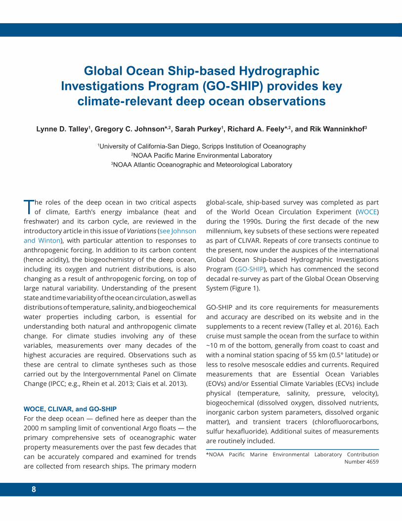
freshwater) and its carbon cycle, are reviewed in the introductory article in this issue of Variations (see Johnson and Winton), with particular attention to responses to anthropogenic forcing. In addition to its carbon content (hence acidity), the biogeochemistry of the deep ocean, including its oxygen and nutrient distributions, is also changing as a result of anthropogenic forcing, on top of large natural variability. Understanding of the present state and time variability of the ocean circulation, as well as distributions of temperature, salinity, and biogeochemical water properties including carbon, is essential for understanding both natural and anthropogenic climate change. For climate studies involving any of these variables, measurements over many decades of the highest accuracies are required. Observations such as these are central to climate syntheses such as those carried out by the Intergovernmental Panel on Climate Change (IPCC; e.g., Rhein et al. 2013; Ciais et al. 2013).

WOCE, CLIVAR, and GO-SHIPFor the deep ocean — defined here as deeper than the 2000 m sampling limit of conventional Argo floats — the primary comprehensive sets of oceanographic water property measurements over the past few decades that can be accurately compared and examined for trends are collected from research ships. The primary modern

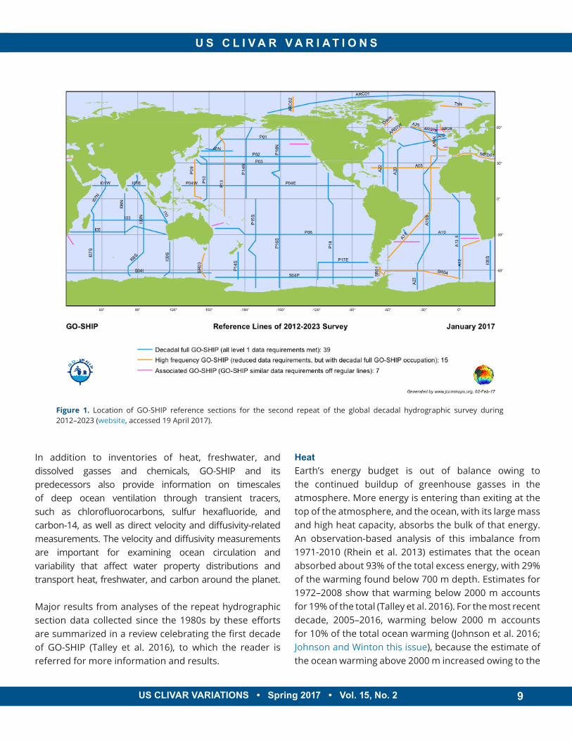
global-scale, ship-based survey was completed as part of the World Ocean Circulation Experiment (WOCE) during the 1990s. During the first decade of the new millennium, key subsets of these sections were repeated as part of CLIVAR. Repeats of core transects continue to the present, now under the auspices of the international Global Ocean Ship-based Hydrographic Investigations Program (GO-SHIP), which has commenced the second decadal re-survey as part of the Global Ocean Observing System (Figure 1).

GO-SHIP and its core requirements for measurements and accuracy are described on its website and in the supplements to a recent review (Talley et al. 2016). Each cruise must sample the ocean from the surface to within ~10 m of the bottom, generally from coast to coast and with a nominal station spacing of 55 km (0.5° latitude) or less to resolve mesoscale eddies and currents. Required measurements that are Essential Ocean Variables (EOVs) and/or Essential Climate Variables (ECVs) include physical (temperature, salinity, pressure, velocity), biogeochemical (dissolved oxygen, dissolved nutrients, inorganic carbon system parameters, dissolved organic matter), and transient tracers (chlorofluorocarbons, sulfur hexafluoride). Additional suites of measurements are routinely included.

*NOAA Pacific Marine Environmental Laboratory Contribution Number 4659

9

U S C L I V A R V A R I A T I O N S

US CLIVAR VARIATIONS • Spring 2017 • Vol. 15, No. 2 9

In addition to inventories of heat, freshwater, and dissolved gasses and chemicals, GO-SHIP and its predecessors also provide information on timescales of deep ocean ventilation through transient tracers, such as chlorofluorocarbons, sulfur hexafluoride, and carbon-14, as well as direct velocity and diffusivity-related measurements. The velocity and diffusivity measurements are important for examining ocean circulation and variability that affect water property distributions and transport heat, freshwater, and carbon around the planet.

Major results from analyses of the repeat hydrographic section data collected since the 1980s by these efforts are summarized in a review celebrating the first decade of GO-SHIP (Talley et al. 2016), to which the reader is referred for more information and results.

HeatEarth’s energy budget is out of balance owing to the continued buildup of greenhouse gasses in the atmosphere. More energy is entering than exiting at the top of the atmosphere, and the ocean, with its large mass and high heat capacity, absorbs the bulk of that energy. An observation-based analysis of this imbalance from 1971-2010 (Rhein et al. 2013) estimates that the ocean absorbed about 93% of the total excess energy, with 29% of the warming found below 700 m depth. Estimates for 1972–2008 show that warming below 2000 m accounts for 19% of the total (Talley et al. 2016). For the most recent decade, 2005–2016, warming below 2000 m accounts for 10% of the total ocean warming (Johnson et al. 2016; Johnson and Winton this issue), because the estimate of the ocean warming above 2000 m increased owing to the

Figure 1. Location of GO-SHIP reference sections for the second repeat of the global decadal hydrographic survey during 2012–2023 (website, accessed 19 April 2017).

10

global sampling of Argo floats. Deep Argo, also discussed in this issue (Zilberman and Roemmich), will allow annual and improved decadal estimates of deep ocean warming when global coverage is achieved.

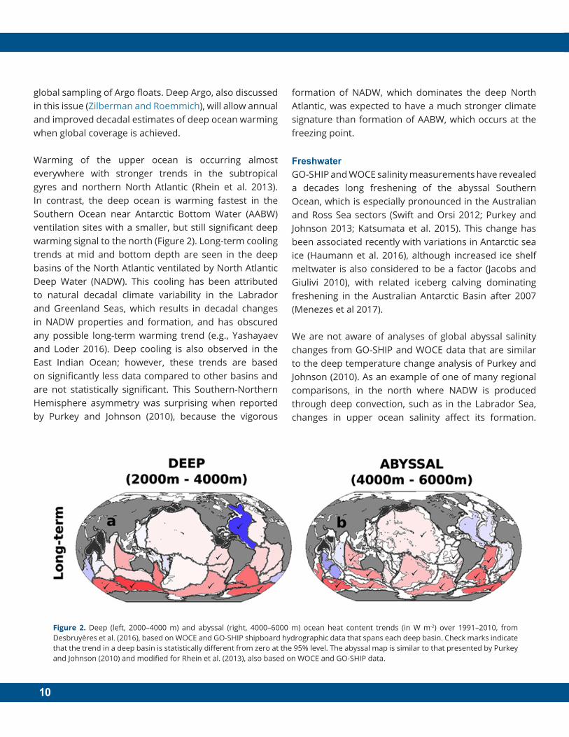
Warming of the upper ocean is occurring almost everywhere with stronger trends in the subtropical gyres and northern North Atlantic (Rhein et al. 2013). In contrast, the deep ocean is warming fastest in the Southern Ocean near Antarctic Bottom Water (AABW) ventilation sites with a smaller, but still significant deep warming signal to the north (Figure 2). Long-term cooling trends at mid and bottom depth are seen in the deep basins of the North Atlantic ventilated by North Atlantic Deep Water (NADW). This cooling has been attributed to natural decadal climate variability in the Labrador and Greenland Seas, which results in decadal changes in NADW properties and formation, and has obscured any possible long-term warming trend (e.g., Yashayaev and Loder 2016). Deep cooling is also observed in the East Indian Ocean; however, these trends are based on significantly less data compared to other basins and are not statistically significant. This Southern-Northern Hemisphere asymmetry was surprising when reported by Purkey and Johnson (2010), because the vigorous

formation of NADW, which dominates the deep North Atlantic, was expected to have a much stronger climate signature than formation of AABW, which occurs at the freezing point.

FreshwaterGO-SHIP and WOCE salinity measurements have revealed a decades long freshening of the abyssal Southern Ocean, which is especially pronounced in the Australian and Ross Sea sectors (Swift and Orsi 2012; Purkey and Johnson 2013; Katsumata et al. 2015). This change has been associated recently with variations in Antarctic sea ice (Haumann et al. 2016), although increased ice shelf meltwater is also considered to be a factor (Jacobs and Giulivi 2010), with related iceberg calving dominating freshening in the Australian Antarctic Basin after 2007 (Menezes et al 2017).

We are not aware of analyses of global abyssal salinity changes from GO-SHIP and WOCE data that are similar to the deep temperature change analysis of Purkey and Johnson (2010). As an example of one of many regional comparisons, in the north where NADW is produced through deep convection, such as in the Labrador Sea, changes in upper ocean salinity affect its formation.

Figure 2. Deep (left, 2000–4000 m) and abyssal (right, 4000–6000 m) ocean heat content trends (in W m-2) over 1991–2010, from Desbruyères et al. (2016), based on WOCE and GO-SHIP shipboard hydrographic data that spans each deep basin. Check marks indicate that the trend in a deep basin is statistically different from zero at the 95% level. The abyssal map is similar to that presented by Purkey and Johnson (2010) and modified for Rhein et al. (2013), also based on WOCE and GO-SHIP data.

11

U S C L I V A R V A R I A T I O N S

US CLIVAR VARIATIONS • Spring 2017 • Vol. 15, No. 2 11

When surface salinity decreases, as it does periodically and mostly driven by natural climate variability (North Atlantic Oscillation), the resulting increased stratification is overcome only when surface temperature is colder, leading to colder, fresher deep convection (Kieke and Yashayaev 2015; Yashayaev and Loder 2016). For the most recent decade, Argo float observations provided the most detailed information, but to connect this to the underlying deeper water properties, and to look at a multi-decade record, research ship observations have been required. These have included the repeated GO-SHIP sections across the Labrador Sea.

CarbonFor the Earth’s carbon budget, GO-SHIP and its predecessors are the primary source of high-quality, global, full water-column ocean carbon data. Changes in ocean carbon inventory and mapping/inventory of anthropogenic carbon extensively use GO-SHIP and WOCE data. The GLODAPv2 synthesis product (Lauvset et al. 2016; Olsen et al. 2016) provides the most recent quality controlled ocean carbon datasets and mapped products, including all GO-SHIP data through 2012.

Based on these inventories and several independent approaches to quantify the amount of carbon that is due to anthropogenic increases, approximately 27% of the net carbon released to the atmosphere by fossil fuel burning and land-use change is sequestered in the ocean, with an increase in the rate of anthropogenic carbon uptake from 2.2 ± 0.5 Pg C yr−1 during the 1990s to approximately 2.6 ± 0.5 Pg C yr−1 during the most recent decade from 2005 to 2014 (Feely et

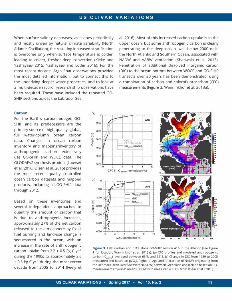
al. 2016). Most of this increased carbon uptake is in the upper ocean, but some anthropogenic carbon is clearly penetrating to the deep ocean, well below 2000 m in the North Atlantic and Southern Ocean, associated with NADW and AABW ventilation (Khatiwala et al. 2013). Penetration of additional dissolved inorganic carbon (DIC) to the ocean bottom between WOCE and GO-SHIP transects over 20 years has been demonstrated, using a combination of carbon and chlorofluorocarbon (CFC) measurements (Figure 3; Wanninkhof et al. 2013a).

Figure 3. Left: Carbon and CFCs along GO-SHIP section A16 in the Atlantic (see Figure 1 for location; Wanninkhof et al. 2013a). (a) CFC profiles and modeled anthropogenic carbon (Canthro), averaged between 63°N and 56°S. (c) Change in DIC from 1989 to 2005 (measured and based on pCO2). Right: (b) Age and (d) fraction of NADW originating from the Denmark Strait Overflow Water (DSOW) between Greenland and Iceland based on CFC measurements; “young” means DSOW with measurable CFCs; from Rhein et al. (2015).

12

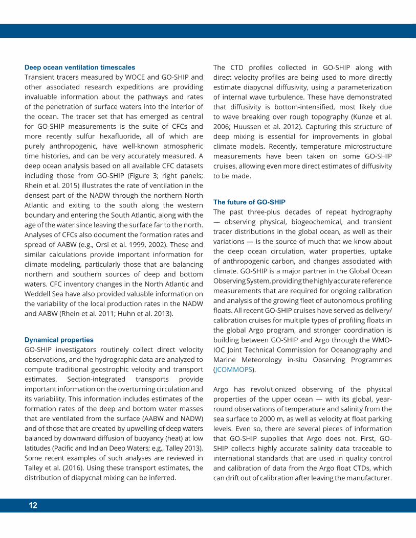
Deep ocean ventilation timescales Transient tracers measured by WOCE and GO-SHIP and other associated research expeditions are providing invaluable information about the pathways and rates of the penetration of surface waters into the interior of the ocean. The tracer set that has emerged as central for GO-SHIP measurements is the suite of CFCs and more recently sulfur hexafluoride, all of which are purely anthropogenic, have well-known atmospheric time histories, and can be very accurately measured. A deep ocean analysis based on all available CFC datasets including those from GO-SHIP (Figure 3; right panels; Rhein et al. 2015) illustrates the rate of ventilation in the densest part of the NADW through the northern North Atlantic and exiting to the south along the western boundary and entering the South Atlantic, along with the age of the water since leaving the surface far to the north. Analyses of CFCs also document the formation rates and spread of AABW (e.g., Orsi et al. 1999, 2002). These and similar calculations provide important information for climate modeling, particularly those that are balancing northern and southern sources of deep and bottom waters. CFC inventory changes in the North Atlantic and Weddell Sea have also provided valuable information on the variability of the local production rates in the NADW and AABW (Rhein et al. 2011; Huhn et al. 2013).

Dynamical propertiesGO-SHIP investigators routinely collect direct velocity observations, and the hydrographic data are analyzed to compute traditional geostrophic velocity and transport estimates. Section-integrated transports provide important information on the overturning circulation and its variability. This information includes estimates of the formation rates of the deep and bottom water masses that are ventilated from the surface (AABW and NADW) and of those that are created by upwelling of deep waters balanced by downward diffusion of buoyancy (heat) at low latitudes (Pacific and Indian Deep Waters; e.g., Talley 2013). Some recent examples of such analyses are reviewed in Talley et al. (2016). Using these transport estimates, the distribution of diapycnal mixing can be inferred.

The CTD profiles collected in GO-SHIP along with direct velocity profiles are being used to more directly estimate diapycnal diffusivity, using a parameterization of internal wave turbulence. These have demonstrated that diffusivity is bottom-intensified, most likely due to wave breaking over rough topography (Kunze et al. 2006; Huussen et al. 2012). Capturing this structure of deep mixing is essential for improvements in global climate models. Recently, temperature microstructure measurements have been taken on some GO-SHIP cruises, allowing even more direct estimates of diffusivity to be made.

The future of GO-SHIP The past three-plus decades of repeat hydrography — observing physical, biogeochemical, and transient tracer distributions in the global ocean, as well as their variations — is the source of much that we know about the deep ocean circulation, water properties, uptake of anthropogenic carbon, and changes associated with climate. GO-SHIP is a major partner in the Global Ocean Observing System, providing the highly accurate reference measurements that are required for ongoing calibration and analysis of the growing fleet of autonomous profiling floats. All recent GO-SHIP cruises have served as delivery/calibration cruises for multiple types of profiling floats in the global Argo program, and stronger coordination is building between GO-SHIP and Argo through the WMO-IOC Joint Technical Commission for Oceanography and Marine Meteorology in-situ Observing Programmes (JCOMMOPS).

Argo has revolutionized observing of the physical properties of the upper ocean — with its global, year-round observations of temperature and salinity from the sea surface to 2000 m, as well as velocity at float parking levels. Even so, there are several pieces of information that GO-SHIP supplies that Argo does not. First, GO-SHIP collects highly accurate salinity data traceable to international standards that are used in quality control and calibration of data from the Argo float CTDs, which can drift out of calibration after leaving the manufacturer.

13

U S C L I V A R V A R I A T I O N S

US CLIVAR VARIATIONS • Spring 2017 • Vol. 15, No. 2 13

Second, GO-SHIP provides quasi-synoptic, full-depth, coast-to-coast sections that are necessary for estimating meridional transports, resolving the boundary currents that Argo does not. GO-SHIP observations through the full depth will be even more critical for the ongoing expansion of Argo to the deep ocean (Deep Argo; Zilberman and Roemmich this issue), where salinity measurement accuracy must be even higher than in the upper ocean because of its often-small variability.

GO-SHIP provides a very accurate high-quality, full-depth, and comprehensive set of ocean biogeochemistry data at a global scale, as well as transient tracer data that can only be measured from ships. However, a growing fleet of biogeochemical Argo floats (BGC-Argo), which, like Argo, provide much higher sampling in space and time, is highly complementary to GO-SHIP. Most BGC-Argo floats are equipped with oxygen and optical sensors that are increasingly stable, and a growing number have nutrient and carbon-related sensors (currently pH). Deep Argo, with its growing fleet, also includes oxygen sensors on some floats. However, all float sensors require in

situ (GO-SHIP) reference data to obtain climate-quality accuracies. GO-SHIP measurements are required for not only for float instrument calibration but also to derive decadally evolving algorithms that connect the limited set of carbon cycle elements measured by the floats to the comprehensive set by GO-SHIP (e.g., Carter et al. 2016; Williams et al. 2017). The two observing systems will remain strongly linked well into the next several decades.

With increased societal interest in the health of ocean ecosystems, future GO-SHIP efforts will incorporate key parameters to address this aspect. This will also dovetail into BGC-Argo and satellite oceanography, where properties such as ocean color, fluorescence, and particulate matter need to be validated and translated to chlorophyll and planktonic species. A proposal was submitted to the Scientific Committee on Oceanic Research (SCOR) in April 2017 to form a working group on the "Integration of Plankton-Observing Sensor Systems to Existing Global Sampling Program" that will address details of augmenting GO-SHIP with key biological variables.

References

Carter, B. R., N. L. Williams, A. R. Gray, and R. A. Feely, 2016: Locally interpolated alkalinity regression for global alkalinity estimation. Limnol. Oceanogr. Methods, 14, 268-277, doi:10.1002/lom3.10087.

Ciais, P., and Coauthors, 2013: Carbon and Other Biogeochemical Cycles. In: Climate Change 2013: The Physical Science Basis. Contribution of Working Group I to the Fifth Assessment Report of the Intergovernmental Panel on Climate Change, T. F. Stocker, and CoAuthors, Eds., Cambridge University Press, 465-570, doi:10.1017/CBO9781107415324.

Desbruyères, D. G., S. G. Purkey, E. L. McDonagh, G. C. Johnson, and B. A. King, 2016: Deep and abyssal ocean warming from 35 years of repeat hydrography. Geophys. Res. Lett., 43, 10356–10365, doi:10.1002/2016GL070413.

Feely, R. A., R. Wanninkhof, B. R. Carter, J. N. Cross, J. T. Mathis, C. L. Sabine, C. E. Cosca, and J. A. Tirnanes, 2016: Global ocean carbon cycle. In State of the Climate in 2015, J. Bulnden, and D. S. Arndt, Eds., Bull. Amer. Meteorol. Soc., 97, S89–S92, doi:10.1175/2016BAMSStateoftheClimate.1.

Haumann, F. A., N. Gruber, M. Munnich, I. Frenger, and S. Kern, 2016: Sea-ice transport driving Southern Ocean salinity and its recent trends. Nature, 537, 89-92, doi:10.1038/nature19101.

Huhn, O., M. Rhien, M. Hoppema, and S. van Heuven, 2013: Decline of deep and bottom water ventilation and slowing down of anthropogenic carbon storage in the Weddell Sea, 1984–2011. Deep Sea Res. Part I: Oceanogr. Res. Pap., 76, 66–84, doi:10.1016/j.dsr.2013.01.005.

Huussen, T. N., A. C. Naveira-Garabato, H. L. Bryden, and E. L. McDonagh 2012: Is the deep Indian Ocean MOC sustained by breaking internal waves? J. Geophys. Res., 117, doi:10.1029/2012JC008236.

Jacobs, S. S., and C. F. Giulivi, 2010: Large multidecadal salinity trends near the Pacific Antarctic continental margin. J. Climate, 23, 4508–4524, doi:10.1175/2010JCLI3284.1.

Johnson, G. C., J. M. Lyman, and N. G. Loeb, 2016: CORRESPONDENCE: Improving estimates of Earth's energy imbalance. Nat. Climate Change, 6, 639–640, doi:10.1038/nclimate3043.

Katsumata, K., H. Nakano, and Y. Kumamoto, 2015: Dissolved oxygen change and freshening of Antarctic Bottom water along 62◦S in the Australian-Antarctic Basin between 1995/1996 and 2012/2013. Deep-Sea Res. II: Top. Stud. Oceangr., 114, 27–38, doi:10.1016/j.dsr2.2014.05.016.

Khatiwala, S., and CoAuthors, 2013: Global ocean storage of anthropogenic carbon. Biogeosci., 10, 2169–2191, doi:10.5194/bg-10-2169-2013.

Kieke, D., and I. Yashayaev, 2015: Studies of Labrador Sea Water formation and variability in the subpolar North Atlantic in the light of international partnership and collaboration. Prog. Oceangr., 132, 220-232, doi:10.1016/j.pocean.2014.12.010.

Kunze, E., E. Firing, J. M. Hummon, T. K. Chereskin, and A. M. Thurnherr, 2006: Global abyssal mixing from lowered ADCP shear and CTD strain profiles. J. Phys. Oceanogr,. 36, 1553–1576, doi: 10.1175/JPO2926.1.

14

Lauvset, S. K., and CoAuthors, 2016: A new global interior ocean mapped clima-tology: the 1x1 GLODAP version 2. Earth Sys. Sci. Data, 8, 325-340, doi: 10.5194/essd-2015-43.

Menezes, V. V., A. M. Macdonald, and C. Schatzman, 2017: Accelerated freshening of Antarctic Bottom Water over the last decade in the southern Indian Ocean. Sci. Adv., 3, doi:10.1126/sciadv.1601426.

Olsen, A., and CoAuthors, 2016: The Global Ocean Data Analysis Project version 2 (GLODAPv2) – an internally consistent data product for the world ocean. Earth Syst. Sci. Data, 8 297-323, doi:10.5194/essd-8-297-2016.

Orsi, A. H., G. C. Johnson, and J. L. Bullister, 1999: Circulation, mixing, and production of Antarctic Bottom Water. Prog. Oceanogr., 43, 55–109, doi:10.1016/S0079-6611(99)00004-X.

Orsi, A. H., W. M. Smethie Jr., and J. L. Bullister, 2002: On the total input of Antarctic waters to the deep ocean: A preliminary estimate from chlorofluorocarbon measurements, J. Geophys. Res., 107, 3101-3114, doi:10.1029/2001JC000976.

Purkey, S. G., and G. C. Johnson, 2010: Warming of global abyssal and deep Southern Ocean waters between the 1990s and 2000s: Contributions to global heat and sea level rise budgets. J. Climate, 23, 6336–6351, doi:10.1175/2010JCLI3682.1.

Purkey, S. G., and G. C. Johnson, 2013: Antarctic Bottom Water warming and freshening: Contributions to sea level rise, ocean freshwater budgets, and global heat gain. J. Climate, 26, 6105–6122, doi:10.1175/JCLI-D-12-00834.1.

Rhein, M., and Coauthors, 2013: Observations: Ocean. Climate Change 2013: The Physical Science Basis. Contribution of Working Group I to the Fifth Assessment Report of the Intergovernmental Panel on Climate Change, T. F. Stocker, and Coauthors, Eds., Cambridge University Press, 255–315.

Rhein M., D. H. Kieke, S. Huttl-Kabus, A. Roessler, C. Mertens, R. Meissner, B. Klein, C. W. Boning, and I. Yashayaev, 2011: Deep water formation, the subpolar gyre, and the meridional overturning circulation in the subpolar North Atlantic. Deep-Sea Res. II, 58, 1819–1832, doi:10.1016/j.dsr2.2010.10.061.

Rhein, M., D. Kieke, and R. Steinfeldt, 2015: Advection of North Atlantic Deep Water from the Labrador Sea to the southern hemisphere. J. Geophys. Res. Oceans, 120, 2471–2487, doi:10.1002/2014JC010605.

Swift J. H., and A. H. Orsi, 2012; Sixty-four days of hydrography and storms: RVIB Nathaniel B. Palmer’s 2011 S04P Cruise. Oceanogr., 25, 54–55, doi: 10.5670/oceanog.2012.74.

Talley, L. D., 2013: Closure of the global overturning circulation through the Indian, Pacific and Southern Oceans: schematics and transports. Oceanogr., 26, 80-97, doi:10.5670/oceanog.2013.07.

Talley, L. D., and Coauthors, 2016: Changes in ocean heat, carbon content, and ventilation: Review of the first decade of global repeat hydrography (GO-SHIP). Ann. Rev. Mar. Sci. 8, 185-215, doi:10.1146/annurev-marine-052915-100829.

Wanninkhof, R., G.-H. Park, T. Takahashi, R. A. Feely, J. L. Bullister, and S. C. Doney, 2013a: Changes in deep-water CO2 concentrations over the last several decades determined from discrete pCO2 measurements. Deep-Sea Res. I, 74, 48–63, doi: 10.1016/j.dsr.2012.12.005.

Wanninkhof, R., and CoAuthors, 2013b: Global ocean carbon uptake: magnitude, variability and trends. Biogeosci. 10, 1983–2000, doi:10.5194/bg-10-1983-2013.

Williams, N. L., R. A. Feely, C. L. Sabine, A. G. Dickson, J. H. Swift, L. D. Talley, and J. L. Russell, 2015: Quantifying anthropogenic carbon inventory changes in the Pacific sector of the Southern Ocean. Mar. Chem., 174, 147-160, doi:10.1016/j.marchem.2015.06.015.

Yashayaev, I., and J. W. Loder, 2016: Recurrent replenishment of Labrador Sea Water and associated decadal-scale variability. J. Geophys. Res., 121, 8095–8114, doi:10.1002/2016JC012046.

Early Bird Registration Closes May 15

15

U S C L I V A R V A R I A T I O N S

US CLIVAR VARIATIONS • Spring 2017 • Vol. 15, No. 2 15

Deep moored observations and OceanSITES

Robert A. Weller1, Albert J. Plueddemann1, Roger Lukas2, Fernando Santiago-Mandujano2, and James T. Potemra2

1Woods Hole Oceanographic Institution

2University of Hawaii

Data acquired from moored sensors is one way that we sample the deep ocean. These sensors provide time

series at fixed locations and are, therefore, well suited to provide observations that can be used in comparison with model results extracted at the same location and depth. These moored time series are essential to accurately quantify temporal variability of temperature, salinity, density, and other properties in the deep ocean. The moored sensors can be sampled rapidly for over a year, with sampling times down to minutes or less, and data from successive deployments at the same location can be merged to yield long time series. Long, well-documented time series of known accuracy provide an excellent benchmark for examining model performance and investigating trends and variability. Moorings also allow instruments to be deployed in vertical arrays that return coincident data to show vertical structures, and diverse sensor types (e.g., salinity, temperature, dissolved oxygen, velocity) installed on the same mooring are used to examine covariability of different properties. The deployment of multiple moorings in a line provides the means to estimate integrated transport of properties across that line.

We start with an overview of the technologies and technical challenges of making observations of the water column using moorings. Then we describe an international effort ― OceanSITES ― to collect time

series data across the global ocean and make those data available across the Internet using standard services and in a common format. OceanSITES is one of the observing elements of the Global Ocean Observing System (GOOS) coordinated by the Joint Technical Commission on Oceanography and Marine Meteorology (JCOMM). In recent years OceanSITES has taken on the challenge of collecting and sharing time series of deep temperature and salinity from moorings. We describe the OceanSITES deep time series project and show an example of data from the site north of Oahu, Hawaii. Data from that site illustrate how we are addressing the challenges and show some early results.

TechniquesInstruments are attached to the mooring line at chosen depths and are typically powered by batteries. Data are stored internally and then downloaded from the instruments when the mooring is recovered. In some cases, inductive telemetry, via the wire rope used for the moorings, is used to collect data from attached instruments and make it available prior to recovery. Other methods, such as collection of data in data capsules that can be released to float to the surface and acoustic communications with ocean gliders, can be used to get access to observations prior to recovery of the mooring. Moorings with surface buoys have the added capability of transmitting data via satellite.

16

There are a wide range of technical challenges beyond engineering successful mooring deployments and recoveries. A fundamental requirement is establishing the depth of the instrument for each measurement. A mooring with subsurface flotation can be displaced downward by the drag of the flow past it, with the depths of instruments attached to the mooring line changing as the mooring responds to the currents. Time series from subsurface moorings thus should include time-varying depth of observation as well as time and the observed quantities (e.g., temperature). Surface moorings typically use a combination of wire rope and chain, from the surface down to about 1000-2000 m, for strength and to address fish bite. Below that, synthetic line provides the ability of the mooring to respond to drag from currents. While the wire rope and chain typically hang close to vertical, the synthetic line has an unknown configuration in the water column, and instruments in that section may move through a large range of depths. One solution is to deploy instruments with pressure sensors to infer the sensor depth using the hydrostatic pressure balance. Another solution is to deploy the deep instrumentation close to the bottom, between the acoustic release and the backup flotation. Backup flotation, typically glass spheres, is placed near the bottom of the mooring and will bring the bottom of the mooring to the surface even if the top flotation is damaged or missing. The short mooring section between the release and the backup flotation is taut and provides a good location for instruments positioned at a fixed depth above the sea floor.

Stability of sensor calibrations is another challenge. Instruments left unattended for a year or more may suffer calibration drift due to internal changes and external fouling. Deep instruments do not experience the sometimes-dramatic biofouling seen in the euphotic zone near the surface, but they do show evidence of becoming coated with a slippery film, perhaps a bacterial coating. Addressing the need to assess the stability of calibrations includes deploying instruments in pairs, overlapping new and old mooring deployments, and using the ship’s CTD to profile near the moorings and/or

to check the moored instruments by clamping them on the CTD cage for a cross-calibration profile before and after mooring recovery. (This then relies upon accurate calibration of the CTD system and careful processing of the data.) There is concern that whatever coating covers the conductivity cell and other sensors at the end of a deployment may be washed off after the anchor release is triggered, and the instruments below the backup flotation are carried rapidly to the surface. Calibration shifts can also occur from mishaps during recovery and thereafter. Thus, although a post-recovery calibration is necessary to ensure consistent measurement accuracy, it may not be sufficient.

OceanSITESThe mission of OceanSITES is to collect, deliver, and promote the use of high-quality data from long-term, high-frequency observations at fixed locations in the open ocean. OceanSITES aims to collect multidisciplinary data worldwide from the full-depth water column as well as the overlying atmosphere. Most sites are occupied by moorings. However, frequent occupation of a site by a ship is also considered to provide the sought-after time series. Since 1999, the international OceanSITES Science Team has shared both data and technical expertise in order to capitalize on the potential of the moorings and ship-based time series. All sites agree to make their data freely available and to submit data in a common format with supporting metadata. OceanSITES data are provided in NetCDF (Network Common Data Form), a machine-independent data format, using Climate-Forecast (CF) conventions. The OceanSITES Data Management Team has developed an implementation of NetCDF for the datasets and provides guidance on preparing and submitting data. OceanSITES members adhere to the CLIVAR data policy and principles, including free and unrestricted exchange.

The OceanSITES data flow is carried out through three organizational units: Principal Investigators (PI), Data Assembly Centers (DAC), and Global Data Assembly Centers (GDAC). In general, a PI provides the data and

17

U S C L I V A R V A R I A T I O N S

US CLIVAR VARIATIONS • Spring 2017 • Vol. 15, No. 2 17

metadata information to a DAC, which applies quality control (QC) checks, reformats this information into NetCDF files with standard conventions and vocabularies, and passes it on to the GDAC. Two GDACs host OceanSITES data and provide standard services for access, including FTP and OPeNDAP/THREDDS. One GDAC is support by the French Research Institute for Exploitation of the Sea (Ifremer/Coriolis) The other GDAC is part of the NOAA National Data Buoy Center (NDBC OceanSITES).

The OceanSITES deep temperature/salinity projectDeep ocean (below 2000 m) observations have been recognized as an important gap in the global ocean observing system (OceanObs09). An international framework is being developed for filling this gap, called the "deep ocean observing strategy." At the December 2011 OceanSITES meeting, it was decided to make use of the many existing OceanSITES platforms in deep water to make an "instant" contribution towards this need and goal. OceanSITES moorings at over 30 sites already carried deep temperature/salinity (T/S) sensors. OceanSITES took on, as a special project, the goals of sustaining and growing the number of OceanSITES equipped to collect deep T/S time series observations. To do so, OceanSITES sought an additional 50 T/S instruments from donors to create a shared pool of instruments to be provided to PIs with existing moorings that were planned to be sustained. To qualify, PIs would accept the obligation to carry out sustained observations, cover the cost of expendables used

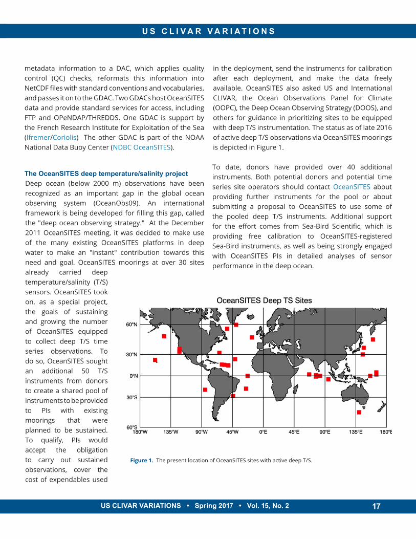
in the deployment, send the instruments for calibration after each deployment, and make the data freely available. OceanSITES also asked US and International CLIVAR, the Ocean Observations Panel for Climate (OOPC), the Deep Ocean Observing Strategy (DOOS), and others for guidance in prioritizing sites to be equipped with deep T/S instrumentation. The status as of late 2016 of active deep T/S observations via OceanSITES moorings is depicted in Figure 1.

To date, donors have provided over 40 additional instruments. Both potential donors and potential time series site operators should contact OceanSITES about providing further instruments for the pool or about submitting a proposal to OceanSITES to use some of the pooled deep T/S instruments. Additional support for the effort comes from Sea-Bird Scientific, which is providing free calibration to OceanSITES-registered Sea-Bird instruments, as well as being strongly engaged with OceanSITES PIs in detailed analyses of sensor performance in the deep ocean.

Figure 1. The present location of OceanSITES sites with active deep T/S.

18

Deep ocean temperature and salinity observations at WHOTS/ALOHATo illustrate some of the technical challenges mentioned above and to show some results, we take a closer look at one set of deep T/S observations.

Established in 1988, a long-term ship-based time series has been maintained at the Hawaii Ocean Time-series (HOT) Station ALOHA (22°45'N, 158°W; Karl and Lukas, 1996). Also at this site is a Woods Hole Oceanographic Institution (WHOI) HOT Site (WHOTS) mooring, which provides sustained, high-quality air-sea fluxes and the associated upper ocean response, since 2004. Successive deployments occur once a year. The WHOTS surface mooring is deployed alternately at two nearby sites on the east (22°46.00'N, 157°54.00'W) and southeast (22°40.00'N, 157° 57.00'W) edges of the Station ALOHA circle (a six nautical mile radius from the ALOHA center). On the WHOTS moorings, two temperature/salinity instruments are located approximately 36 m above the seafloor, which is ~4693 m deep for the east site and ~4758 m deep for the southeast site. Several days of overlap of the new mooring with the old mooring support cross-calibrations.

Located nearby is the University of Hawaii's ALOHA Cabled Observatory (ACO), 1.2 km SSW of ALOHA center on the seafloor 4728 m below the surface (Howe et al., 2015). The ACO measures ocean sounds and continuous

observations of pressure, temperature, salinity, ocean currents, and ocean sounds. It is cabled to shore, so the data are continuously available in real-time and made publicly available.

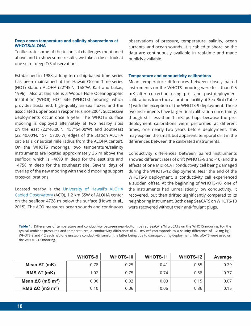
Temperature and conductivity calibrationsMean temperature differences between closely paired instruments on the WHOTS mooring were less than 0.5 mK after correction using pre- and post-deployment calibrations from the calibration facility at Sea-Bird (Table 1) with the exception of the WHOTS-9 deployment. Those two instruments have larger final calibration uncertainty, though still less than 1 mK, perhaps because the pre-deployment calibrations were performed at different times, one nearly two years before deployment. This may explain the small, but apparent, temporal drift in the differences between the calibrated instruments.

Conductivity differences between paired instruments showed different rates of drift (WHOTS-9 and -10) and the effects of one MicroCAT conductivity cell being damaged during the WHOTS-12 deployment. Near the end of the WHOTS-9 deployment, a conductivity cell experienced a sudden offset. At the beginning of WHOTS-10, one of the instruments had unrealistically low conductivity. It recovered, but then drifted significantly compared to its neighboring instrument. Both deep SeaCATS on WHOTS-10 were recovered without their anti-foulant plugs.

Table 1. Differences of temperature and conductivity between near-bottom paired SeaCATs/MicroCATs on the WHOTS mooring. For the typical ambient pressures and temperatures, a conductivity difference of 0.1 mS m-1 corresponds to a salinity difference of 1.2 mg kg-1. WHOTS-9 and -12 each had one unstable conductivity sensor, the latter being due to damage during deployment. MicroCATS were used on the WHOTS-12 mooring.

WHOTS-9 WHOTS-10 WHOTS-11 WHOTS-12 AverageMean ΔT (mK) 0.78 0.25 -0.41 0.55 0.29

RMS ΔT (mK) 1.02 0.75 0.74 0.58 0.77

Mean ΔC (mS m-1) 0.06 0.02 0.03 0.15 0.07

RMS ΔC (mS m-1) 0.10 0.06 0.06 0.36 0.15

19

U S C L I V A R V A R I A T I O N S

US CLIVAR VARIATIONS • Spring 2017 • Vol. 15, No. 2 19

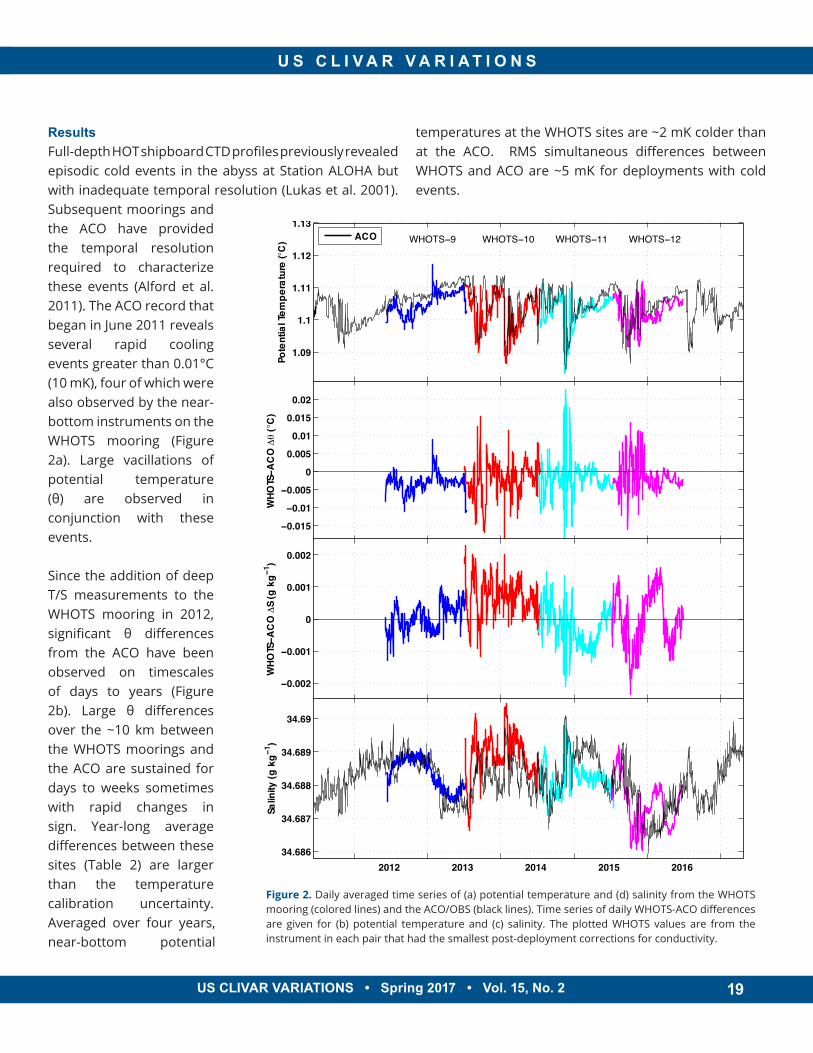
ResultsFull-depth HOT shipboard CTD profiles previously revealed episodic cold events in the abyss at Station ALOHA but with inadequate temporal resolution (Lukas et al. 2001). Subsequent moorings and the ACO have provided the temporal resolution required to characterize these events (Alford et al. 2011). The ACO record that began in June 2011 reveals several rapid cooling events greater than 0.01°C (10 mK), four of which were also observed by the near-bottom instruments on the WHOTS mooring (Figure 2a). Large vacillations of potential temperature (θ) are observed in conjunction with these events.

Since the addition of deep T/S measurements to the WHOTS mooring in 2012, significant θ differences from the ACO have been observed on timescales of days to years (Figure 2b). Large θ differences over the ~10 km between the WHOTS moorings and the ACO are sustained for days to weeks sometimes with rapid changes in sign. Year-long average differences between these sites (Table 2) are larger than the temperature calibration uncertainty. Averaged over four years, near-bottom potential

temperatures at the WHOTS sites are ~2 mK colder than at the ACO. RMS simultaneous differences between WHOTS and ACO are ~5 mK for deployments with cold events.

Figure 2. Daily averaged time series of (a) potential temperature and (d) salinity from the WHOTS mooring (colored lines) and the ACO/OBS (black lines). Time series of daily WHOTS-ACO differences are given for (b) potential temperature and (c) salinity. The plotted WHOTS values are from the instrument in each pair that had the smallest post-deployment corrections for conductivity.

1.09

1.1

1.11

1.12

1.13

Pote

ntia

l Tem

pera

ture

(°C

)

WHOTS−9 WHOTS−10 WHOTS−11 WHOTS−12ACO

−0.015

−0.01

−0.005

0

0.005

0.01

0.015

0.02

WHO

TS−A

CO

∆θ

(°C

)

−0.002

−0.001

0

0.001

0.002

WHO

TS−A

CO

∆S

(g k

g−1 )

2012 2013 2014 2015 2016 34.686

34.687

34.688

34.689

34.69

Salin

ity (g

kg−

1 )

20

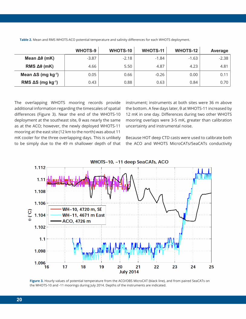
The overlapping WHOTS mooring records provide additional information regarding the timescales of spatial differences (Figure 3). Near the end of the WHOTS-10 deployment at the southeast site, θ was nearly the same as at the ACO; however, the newly deployed WHOTS-11 mooring at the east site (12 km to the north) was about 11 mK cooler for the three overlapping days. This is unlikely to be simply due to the 49 m shallower depth of that

instrument; instruments at both sites were 36 m above the bottom. A few days later, θ at WHOTS-11 increased by 12 mK in one day. Differences during two other WHOTS mooring overlaps were 3-5 mK, greater than calibration uncertainty and instrumental noise. Because HOT deep CTD casts were used to calibrate both the ACO and WHOTS MicroCATs/SeaCATs conductivity

Table 2. Mean and RMS WHOTS-ACO potential temperature and salinity differences for each WHOTS deployment.

WHOTS-9 WHOTS-10 WHOTS-11 WHOTS-12 AverageMean Δθ (mK) -3.87 -2.18 -1.84 -1.63 -2.38

RMS Δθ (mK) 4.66 5.50 4.87 4.23 4.81

Mean ΔS (mg kg-1) 0.05 0.66 -0.26 0.00 0.11

RMS ΔS (mg kg-1) 0.43 0.88 0.63 0.84 0.70

Figure 3. Hourly values of potential temperature from the ACO/OBS MicroCAT (black line), and from paired SeaCATs on the WHOTS-10 and -11 moorings during July 2014. Depths of the instruments are indicated.

21

U S C L I V A R V A R I A T I O N S

US CLIVAR VARIATIONS • Spring 2017 • Vol. 15, No. 2 21

records, salinity across the WHOTS deployments (Figure 2d) is constrained to be the same as the ACO. This is reflected in the deployment-mean WHOTS-ACO salinity differences (Table 2), which are all less than 0.66 mg kg-1, with RMS differences of <1 mg kg-1. Shorter-term differences as large as 2 mg kg-1 are observed (Figure 2c).

DiscussionAbyssal ocean temperature signals at Station ALOHA are an order of magnitude larger than the calibration uncertainty of 0.5-1 mK and the instrumental noise (≤1 mK). Conductivity calibration uncertainty leads to salinity uncertainty of ~1 mg kg-1.

The episodic cooling events at Station ALOHA complicate the quantification of long-term climate trends in near-bottom temperatures. From the minimum temperature of the 2011 cold event, temperature increased by 20 mK to mid-2013. Ranging over 30 mK subsequently, temperature in January 2017 was nearly the same as in January 2012. Salinity likewise was essentially the same for these two times as determined by the calibrated ACO MicroCAT, though ranging over 4 mg kg-1.

The effects of bottom topography on the abyssal dynamics gives rise to significant potential temperature differences over of order 10-12 km that are as large as 20 mK, and sustained at levels ≥5 mK for days to weeks. Lagged correlations of θ also reveal ~0.13 m s-1 westward propagation of signals, much larger than the average currents observed at the ACO. So the ocean "noise" on these time and space scales is not simply random, complicating the quantification of climate trends.

The combination of moored instruments, a seafloor cabled observatory, and repeat shipboard CTD profiles at Station ALOHA is uniquely able to identify these multiple scales of variability, and quantify them in relation to instrumental uncertainties.

ConclusionsTime series in the deep ocean being collected from moorings provide important insight into the temporal variability of the deep ocean. These time series serve as valuable benchmarks for examining the realism of models in replicating the temperature and salinity variations of the deep ocean, and they motivate work to improve models. The sensors deployed on moorings are recovered and recalibrated, as opposed to those on the deep profiling floats, and offer the opportunity to investigate and quantify sensor performance. In addition, the temporal sampling from moorings at specific sites done at the moorings complements the spatial sampling achieved by repeat hydrography. Thus, time series are an essential component of any deep ocean observing system. To answer the need OceanSITES has embarked on a program to equip existing moorings around the world with deep T/S sensors and is making these data freely available at the OceanSITES GDACS at Ifremer and at NDBC. Examples from ongoing observations at the WHOTS site point to potential temperature being observed with existing instrumentation to an accuracy of better than 1 mK, and salinity to 1-2 mg kg-1 with periodic nearby high-quality CTD casts from ships.

References

Alford, M.H., R. Lukas, B. Howe, A. Pickering, and F. Santiago-Mandujano, 2011: Moored observations of episodic abyssal flow and mixing at station ALOHA. Geophys. Res. Lett., 38, doi:10.1029/2011GL048075.

Howe, B. M., F. K. Duennebier, and R. Lukas, 2015: The ALOHA Cabled Observatory. In Seafloor Observatories: A new vision of the Earth from the Abyss, Eds. P. Favali, L. Beranzoli and A. De Santis, Springer-Praxis Publishing, 439-463, doi:10.1007/978-3-642-11374-1.

Karl, D. M., and R. Lukas, 1996: The Hawaii Ocean Time-series (HOT) Program: Background, rationale and field implementation. Deep-Sea Res. II, 43, 129-156, doi:10.1016/0967-0645(96)00005-7.

Lukas, R., F. Santiago-Mandujano, F. Bingham and A. Mantyla, 2001: Cold bottom water events observed in the Hawaii Ocean Time-series: Implications for vertical mixing. Deep-Sea Res. I, 48, 995-1021, doi:10.1016/S0967-0637(00)00078-9.

22

Since their launch in early 2002, the twin satellites of the Gravity Recovery and Climate Experiment (GRACE)

have been providing global maps of Earth’s varying gravity field nearly continuously every month. The data record now spans more than 15 years of global surface mass change observations, allowing precise tracking of the redistribution and cycling of water between the land, atmosphere, and oceans.  

This tracking of mass transport over the oceans via the associated gravity field changes enable two key measurements of oceanographic variability and processes. First, GRACE makes it possible to quantify large-scale ocean mass and sea level changes (Chambers et al. 2004; Johnson and Chambers 2013), such as arising from melting land ice (e.g., van den Broeke et al. 2016) and continental water storage changes related to El Niño, La Niña, and other climatic variations  (e.g., Boening et al. 2012; Fasullo et al. 2013). GRACE observations have been extensively used to assess the contribution of ocean mass changes to the global sea level budget. The combination of gravimetry (ocean mass) and altimetry (sea level) yields an indirect estimate of full-depth ocean warming as a residual between sea surface height and ocean mass. By comparing these full-depth estimates against the direct temperature observations in the upper 2000 m from the Argo float network, the deep ocean contribution to steric sea level from below 2000 m can be estimated.

Second, GRACE makes it possible to measure monthly bottom pressure changes associated with currents (from geostrophic balance). This can currently be done over large-scales (approximately 300 km) due to a particular correlated error signature prevalent in GRACE gravity maps that requires post-processing algorithms that effectively reduce noise (Swenson and Wahr 2006; Chambers and Bonin 2012). Thus, most regional studies using GRACE bottom pressure for ocean current studies have done so at basin-scales, combining observations of dynamic sea level and surface wind stress with bottom pressure observations to infer the ocean’s dynamic forced response. More recently, and in particular with the development of advanced (so-called mass concentration, or ‘‘mascon”) processing methods (Watkins et al. 2015; Landerer et al. 2015), inferring bottom pressure anomalies and pressure gradients associated with deep currents has become more feasible (discussed below).

The 15-year data record of ocean mass and bottom pressureGRACE gravity measurements are used to infer changes in mass (Wahr et al. 1998). Over the ocean, this will represent the mass change of the entire water column or, equivalently, the pressure change at the sea floor. Since pressure and water height are related through hydrostatic equilibrium, bottom pressure anomalies are

Remote sensing of bottom pressure from GRACE satellites

Cecilia Peralta-Ferriz1, Felix W. Landerer2, Don P. Chambers3, Denis Volkov4, and William Llovel5

1University of Washington

2NASA Jet Propulsion Laboratory3University of South Florida

4NOAA Atlantic Oceanographic and Meteorological Laboratory5University of Bristol

23

U S C L I V A R V A R I A T I O N S

US CLIVAR VARIATIONS • Spring 2017 • Vol. 15, No. 2 23

commonly expressed in terms of equivalent sea level (or water thickness), using an average density (typically 1027 kg m-3 for ocean studies).

The largest monthly ocean bottom pressure variations are at high-latitudes and in coastal regions, typically reaching up to 4 or 5 cm RMS in equivalent sea level. However, compared to monthly sea surface height variability, which can often exceed 30 cm RMS in western boundary currents and the Southern Ocean, bottom pressure variations at high latitudes and elsewhere are relatively small. Although bottom pressure variability is generally smaller than that of the total sea level on short time scales, with the 15-year record from GRACE now available, it has been discovered that there are regions where interannual changes in ocean bottom pressure (periods from 1-5 years) explain a significant fraction of total sea level. These areas include the northwestern Pacific (Chambers and Willis 2008; Chambers 2011; Cheng et al. 2013) as well as regions in the Northeast Atlantic, South Pacific, and South Indian Ocean (Piecuch et al. 2013; Ponte and Piecuch 2014).

There are also significant decadal-scale changes in ocean bottom pressure during the GRACE period (Figure 1a). The trend in the North Pacific has been linked to decadal changes in the zonal wind-stress north and south of 40°N (Chambers 2011; Cheng et al. 2013), most likely related to the Pacific Decadal Oscillation. The Arctic mass trend has been linked to a change in the circulation related to the Arctic Oscillation (Morison et al. 2012; Peralta-Ferriz et al. 2014; Armitage et al. 2016). The trends in the Southern Ocean have been linked to fluctuations in the Southern Hemisphere

winds, where winds over the South Indian Ocean and South Atlantic were decreasing from 2003 until 2012, while winds over the South Pacific were increasing over the same time (Makowski et al. 2015).

When averaged over the entire ocean, ocean mass variations explain a significant fraction (~60%) of interannual global mean sea level (Figure 1b; Chambers et al. 2017). The large trend in ocean mass is caused primarily by melting land ice (glaciers and ice sheets),

Figure 1. (a) Bottom pressure trends (in mm yr-1) as observed with GRACE from 2005 to 2014. The global mean trend of 1.6 mm yr-1 has been removed. Note that the area in the Eastern Indian Ocean affected by the 2004 Sumatran earthquake has been set to zero here. (b) Global mean sea level (GMSL) from altimetry, ocean mass component from GRACE, and thermosteric component from Argo for 2005-2015 (modified from Chambers et al. 2017).

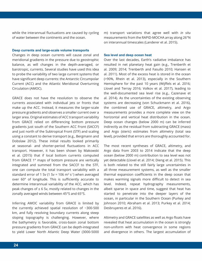
24

while the interannual fluctuations are caused by cycling of water between the continents and the ocean.

Deep currents and large-scale volume transportsChanges in deep ocean currents will cause zonal and meridional gradients in the pressure due to geostrophic balance, as will changes in the depth-averaged, or barotropic, currents. Several studies have used this idea to probe the variability of two large current systems that have significant deep currents: the Antarctic Circumpolar Current (ACC) and the Atlantic Meridional Overturning Circulation (AMOC).

GRACE does not have the resolution to observe the currents associated with individual jets or fronts that make up the ACC. Instead, it measures the larger-scale pressure gradients and observes a smaller current over a larger area. Original estimates of ACC transport variability from GRACE relied on differencing bottom pressure gradients just south of the Southern ACC Front (SACCF) and just north of the Subtropical Front (STF) and scaling using a constant to derive transport (e.g., Bergmann and Dobslaw 2012). These initial results looked primarily at seasonal- and shorter-period fluctuations in ACC transport. However, it has been shown by Makowski et al. (2015) that if local bottom currents computed from GRACE 1° maps of bottom pressure are vertically integrated and summed from the SACCF to the STF, one can compute the total transport variability with a standard error of 1 Sv (1 Sv = 106 m3 s-1) when averaged over 60° of longitude. This is sufficiently accurate to determine interannual variability of the ACC, which has peak changes of ± 6 Sv, mostly related to changes in the zonally averaged winds between 45°S and 65°S.

Inferring AMOC variability from GRACE is limited by the currently achieved spatial resolution of ~300-500 km, and fully resolving boundary currents along steep sloping topography is challenging. However, where the bathymetry is favorable, cross-basin zonal bottom pressure gradients from GRACE can be depth-integrated to yield Lower North Atlantic Deep Water (3000-5000

m) transport variations that agree well with in situ measurements from the RAPID-MOCHA array along 26°N on interannual timescales (Landerer et al. 2015).

Sea level and deep ocean heatOver the last decades, Earth’s radiative imbalance has resulted in net planetary heat gain (e.g., Trenberth et al. 2009; 2014; Trenberth and Fasullo 2010; Hansen et al. 2011). Most of the excess heat is stored in the ocean (>90%, Rhein et al. 2013), especially in the Southern Hemisphere for the past 10 years (Wijffels et al. 2016; Llovel and Terray 2016; Volkov et al. 2017), leading to the well-documented sea level rise (e.g., Cazenave et al. 2014). As the uncertainties of the existing observing systems are decreasing (von Schuckmann et al. 2016), the combined use of GRACE, altimetry, and Argo measurements provides a more complete view on the horizontal and vertical heat distribution in the ocean. Deep ocean changes (below 2000 m) can be inferred indirectly as the residual from subtracting GRACE (mass) and Argo (steric) estimates from altimetry (total sea level), provided that errors are thoroughly accounted for.

The most recent syntheses of GRACE, altimetry, and Argo data from 2003 to 2014 indicate that the deep ocean (below 2000 m) contribution to sea level was not yet detectable (Llovel et al. 2014; Dieng et al. 2015). This is both related to the still fairly large uncertainties in all three measurement systems, as well as the smaller thermal expansion coefficients in the deep ocean that makes warming signals more difficult to detect in sea level. Indeed, repeat hydrography measurements, albeit sparse in space and time, suggest that heat has started to penetrate into the deeper layers of the ocean, in particular in the Southern Ocean (Purkey and Johnson 2010; Abraham et al. 2013; Purkey et al. 2014; Desbruyeres et al. 2016).

Altimetry and GRACE satellites as well as Argo floats have revealed that heat accumulation in the ocean is strongly non-uniform with heat convergence in some regions and divergence in others. The largest accumulation of

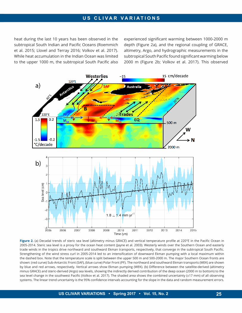
25

U S C L I V A R V A R I A T I O N S

US CLIVAR VARIATIONS • Spring 2017 • Vol. 15, No. 2 25

heat during the last 10 years has been observed in the subtropical South Indian and Pacific Oceans (Roemmich et al. 2015; Llovel and Terray 2016; Volkov et al. 2017). While heat accumulation in the Indian Ocean was limited to the upper 1000 m, the subtropical South Pacific also

experienced significant warming between 1000-2000 m depth (Figure 2a), and the regional coupling of GRACE, altimetry, Argo, and hydrographic measurements in the subtropical South Pacific found significant warming below 2000 m (Figure 2b; Volkov et al. 2017). This observed

Figure 2. (a) Decadal trends of steric sea level (altimetry minus GRACE) and vertical temperature profile at 220°E in the Pacific Ocean in 2005-2014. Steric sea level is a proxy for the ocean heat content (Jayne et al. 2003). Westerly winds over the Southern Ocean and easterly trade winds in the tropics drive northward and southward Ekman transports, respectively, that converge in the subtropical South Pacific. Strengthening of the wind stress curl in 2005-2014 led to an intensification of downward Ekman pumping with a local maximum within the dashed box. Note that the temperature scale is split between the upper 500 m and 500-2000 m. The major Southern Ocean fronts are shown: (red curve) Sub-Antarctic Front (SAF), (blue curve) Polar Front (PF). The northward and southward Ekman transports (MEK) are shown by blue and red arrows, respectively. Vertical arrows show Ekman pumping (WEK). (b) Difference between the satellite-derived (altimetry minus GRACE) and steric-derived (Argo) sea levels, showing the indirectly derived contribution of the deep ocean (2000 m to bottom) to the sea level change in the southwest Pacific (Volkov et al. 2017). The shaded area shows the combined uncertainty (±17 mm) of all observing systems. The linear trend uncertainty is the 95% confidence intervals accounting for the slope in the data and random measurement errors.

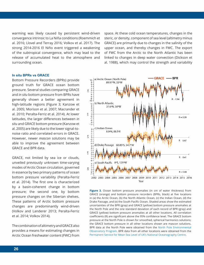
26

warming was likely caused by persistent wind-driven convergence intrinsic to La Niña conditions (Roemmich et al. 2016; Llovel and Terray 2016; Volkov et al. 2017). The strong 2014-2016 El Niño event triggered a weakening of the subtropical convergence, which may lead to the release of accumulated heat to the atmosphere and surrounding ocean.

In situ BPRs vs GRACEBottom Pressure Recorders (BPRs) provide ground truth for GRACE ocean bottom pressure. Several studies comparing GRACE and in situ bottom pressure from BPRs have generally shown a better agreement in high-latitude regions (Figure 3; Kanzow et al. 2005; Morison et al. 2007; Macrander et al. 2010; Peralta-Ferriz et al. 2014). At lower latitudes, the larger differences between in situ and GRACE bottom pressure (Kanzow et al. 2005) are likely due to the lower signal-to-noise ratio and correlated errors in GRACE. However, newer mascon solutions may be able to improve the agreement between GRACE and BPR data.

GRACE, not limited by sea ice or clouds, unveiled previously unknown time-varying modes of Arctic Ocean circulation, governed in essence by two primary patterns of ocean bottom pressure variability (Peralta-Ferriz et al. 2014). The first one is characterized by a basin-coherent change in bottom pressure; the second one, by bottom pressure changes on the Siberian shelves. These patterns of Arctic bottom pressure changes are predominantly wind-driven (Volkov and Landerer 2013; Peralta-Ferriz et al. 2014; Volkov 2014).

The combination of altimetry and GRACE also provides a means for estimating changes in Arctic Ocean freshwater content (FWC) from

space. At these cold ocean temperatures, changes in the steric, or density, component of sea level (altimetry minus GRACE) are primarily due to changes in the salinity of the upper ocean, and thereby changes in FWC. The export of FWC from the Arctic to the North Atlantic has been linked to changes in deep water convection (Dickson et al. 1988), which may control the strength and variability

Figure 3. Ocean bottom pressure anomalies (in cm of water thickness) from GRACE (orange) and bottom pressure recorders (BPRs, black) at five locations in (a) the Arctic Ocean, (b) the North Atlantic Ocean, (c) the Indian Ocean, (d) the Drake Passage, and (e) the South Pacific Ocean. Shaded areas show the estimated uncertainties of the BPR (gray) and GRACE (yellow) bottom pressure anomalies at the North Pole and the one standard deviation of each record of BPR (gray) and GRACE (yellow) bottom pressure anomalies at all other locations. All correlation coefficients (R) are significant above the 95% confidence level. The GRACE bottom pressure at the North Pole is shown for smoothed, spherical harmonics solutions; the GRACE bottom pressure in all other locations shown are mascon solutions. BPR data at the North Pole were obtained from the North Pole Environmental Observatory Program. BPR data from all other locations were obtained from the Permanent Service for Mean Sea Level of UK’s National Oceanography Centre.

27

U S C L I V A R V A R I A T I O N S

US CLIVAR VARIATIONS • Spring 2017 • Vol. 15, No. 2 27

of the AMOC (Rahmstorf et al. 2015). Studies have shown a significant increase in satellite-derived Arctic FWC in the Canada Basin from 2004 to 2008 (Giles et al. 2012) that was mostly compensated by a FWC decrease in the Siberian shelves and Eurasian basin (Morison et al. 2012), resulting in a net small, but significant, increase in FWC in the entire Arctic basin (Morison et al. 2012; Rabe et al. 2014).

The future: GRACE Follow-On The two GRACE satellites have exceeded their intended lifetime by a factor of three. This long and stable data record has enabled many insights into regional and global ocean dynamical as well as water and energy cycle processes. The monthly ocean mass and bottom pressure observations derived from the time-variable gravity measurements provide a unique view into the

deep ocean that is otherwise sparsely sampled with direct observations. As the current GRACE mission approaches its end, the GRACE Follow-On satellites are scheduled to launch in early 2018 to continue the successful data record. While the core focus of GRACE Follow-On is on continuity, a new, more precise laser ranging system will be tested to improve measurement accuracies and sensitivities. In conjunction with altimetric sea surface height and in situ hydrographic observations such as from Argo profiling floats and ice-tethered profiler buoys, and in situ bottom pressure data from BPRs, GRACE Follow-On will answer crucial questions about deep ocean warming and provide further insights into large-scale volume transports and their spatial and temporal evolution and coherence.

References

Abraham, J. P., and Coauthors, 2013: A review of global ocean temperature observations: Implications for ocean heat content estimates and climate change. Rev. Geophys., 51, 450–483, doi:10.1002/rog.20022.

Armitage, T. W. K., S. Bacon, A. L. Ridout, S. F. Thomas, Y. Aksenov, and D. J. Wingham, 2016: Arctic sea surface height variability and change from satellite radar altimetry and GRACE, 2003–2014. J. Geophys. Res. - Oceans, 121, 4303–4322, doi:10.1002/2015JC011579.

Boening, C., J. K. Willis, F. W. Landerer, R. S. Nerem, and J. Fasullo, 2012: The 2011 La Niña: So strong, the oceans fell. Geophys. Res. Lett., 39, doi:10.1029/2012GL053055.

Bergmann, I., and H. Dobslaw, 2012: Short-term transport variability of the Antarctic circumpolar current from satellite gravity observations. J. Geophys. Res., 117, doi:10.1029/2012JC007872.

Cazenave, A. and G. L. Cozannet, 2014: Sea level rise and its coastal impacts. Earth's Future, 2, 15–34, doi:10.1002/2013EF000188.

Chambers, D. P., 2011: ENSO-correlated fluctuations in ocean bottom pressure and wind-stress curl in the North Pacific. Ocean Sci., 7, 685-692, doi:10.5194/os-7-685-2011.

Chambers D. P., J. Wahr, and R. S. Nerem, 2004: Preliminary observations of global ocean mass variations with GRACE. Geophys. Res. Lett., 31, doi:10.1029/2004GL020461.

Chambers, D. P. and J. K. Willis, 2008: Analysis of large-scale ocean bottom pressure variability in the North Pacific. J. Geophys. Res., 113, doi:10.1029/2008JC004930.

Chambers, D. P. and J. A. Bonin, 2012: Evaluation of Release-05 GRACE time-variable gravity coefficients over the ocean. Ocean Sci., 8, 1–10, doi:10.5194/os-8-1-2012.

Chambers, D. P., A. Cazenave, N. Champollion, H. Dieng, W. Llovel, R. Forsberg, K. von Schuckmann, and Y. Wada, 2017: Evaluation of

the global mean sea level budget between 1993 and 2014. Surv. Geophys., 38, 309-327, doi:10.1007/s10712-016-9381-3.

Cheng, X., L. Li, Y. Du, J. Wang, and R.-X. Huang, 2013: Mass-induced sea level change in the northwestern North Pacific and its contribution to total sea level change. Geophys. Res. Lett., 40, doi:10.1002/grl.50748.

Desbruyères, D. G., S. Purkey, E. L. McDonagh, G. C. Johnson, and B. A. King, 2016: Deep and abyssal ocean warming from 35 years of repeat hydrography. Geophys. Res. Lett., 43, 10,356–10,365, doi:10.1002/2016GL070413.

Dickson, R. R., J. Meincke, S-A Malmberg and A. J. Lee, 1988: The “great salinity anomaly” in the Northern North Atlantic 1968-1982. Prog. Oceanogr., 20, 103-151, doi:10.1016/0079-6611(88)90049-3.

Dieng, H. B., A. Cazenave, K. von Schuckmann, M. Ablain and B. Meyssignac, 2015: Sea level budget over 2005–2013: missing contributions and data errors. Ocean Sci., 11, 789–802, doi:10.5194/os-11-789-2015.

Fasullo, J. T., C. Boening, F. W. Landerer, and R. S. Nerem, 2013: Australia's unique influence on global sea level in 2010–2011. Geophys. Res. Lett., 40, 4368–4373, doi:10.1002/grl.50834.

Giles, K. A., S. W. Laxon, A. L. Ridout, D. K. Wingham and S. Bacon, 2012: Western Arctic Ocean freshwater storage increased by wind-driven spin-up of the Beaufort Gyre. Nat. Geosci., 5, 194-197, doi:10.1038/ngeo1379.

Hansen, J., M. Sato, P. Kharecha, and K. von Schuckmann, 2011: Earth's energy imbalance and implications. Atmos. Chem. Phys., 11, 13421-13449, doi:10.5194/acp-11-13421-2011.

Jayne, S. R., J. M. Wahr, and F. O. Bryan, 2003: Observing ocean heat content using satellite gravity and altimetry. J. Geophys. Res., 108, doi:10.1029/2002JC001619.

28

Johnson, G. F., and D. P. Chambers, 2013: Ocean bottom pressure seasonal cycles and decadal trends from GRACE Release-05: Ocean circulation implications. J. Geophys. Res. Oceans, 118, 4228-4240, doi:10.1002/jgrc.20307.

Kanzow, T., F. Flechtner, A. Chave, R. Schmidt, P. Schwintzer, and U. Send, 2005: Seasonal variation of ocean bottom pressure from Gravity Recovery and Climate Experiment (GRACE): Local validation and global patterns. J. Geophys. Res., 110, doi:10.1029/2004JC002772.

Landerer, F. W., D. N. Wiese, K. Bentel, C. Boening, and M. M. Watkins, 2015: North Atlantic meridional overturning circulation variations from GRACE ocean bottom pressure anomalies. Geophys. Res. Lett., 42, doi:10.1002/2015GL065730.

Llovel, W., J. K. Willis, F. W. Landerer, and I. Fukumori, 2014: Deep-ocean contribution to sea level and energy budget not detectable over the past decade. Nat. Climate Change, 4, 1031-1035, doi:10.1038/NCLIMATE2387.

Llovel, W., and L. Terray, 2016: Observed southern upper-ocean warming over 2005–2014 and associated mechanisms. Environ. Res. Lett., 11, doi:10.1088/1748-9326/11/12/124023.

Macrander, A., C. Boening, O. Boebel, and J. Schroeter, 2010: Validation of GRACE gravity fields by in-situ data of ocean bottom pressure. System Earth via Geodetic-Geophysical Space Techniques, Advanced Technologies in Earth Sciences, F. Flechtner et al. (Eds), Springer, 169-185, doi:10.1007/978-3-642-10228-8_14.

Makowski, J. K., D. P. Chambers, and J. A. Bonin, 2015: Using ocean bottom pressure from the gravity recovery and climate experiment (GRACE) to estimate transport variability in the southern Indian Ocean. J. Geophys. Res. Oceans, 120, 4245-4259, doi:10.1002/2014JC010575.

Morison, J., J. Wahr, R. Kwok, and C. Peralta-Ferriz, 2007: Recent trends in Arctic Ocean mass distribution revealed by GRACE. Geophys. Res. Lett., 34, doi:10.1029/2006GL029016.

Morison, J., R. Kwok, C. Peralta-Ferriz, M. Alkire, I. Rigor, R. Andersen, and M. Steele, 2012: Changing Arctic Ocean freshwater pathways. Nature, 481, 66–70, doi:10.1038/nature10705.

Peralta-Ferriz, C., J. H. Morison, J. M. Wallace, J. A. Bonin, and J. Zhang, 2014: Arctic Ocean circulation patterns revealed by GRACE. J. Climate, 27, 1445–1468, doi:10.1175/JCLI-D-13-00013.1.

Piecuch, C. G., K. J. Quinn, and R. M. Ponte, 2013: Satellite-derived interannual ocean bottom pressure variability and its relation to sea level. Geophys. Res. Lett., 40, doi:10.1002/grl.50549.

Ponte, R. M., and C. G. Piechuch, 2014: Interannual bottom pressure signals in the Australian–Antarctic and Bellingshausen Basins. J. Phys. Ocean., 44, 1456-1465, doi:10.1175/JPO-D-13-0223.1.

Purkey, S. G., and G. C. Johnson, 2010: Warming of global abyssal and deep Southern Ocean waters between the 1990s and 2000s: Contributions to global heat and sea level budgets. J. Climate, 23, 6336–6351, doi:10.1175/2010JCLI3682.1.

Purkey, S. G., G. C. Johnson, and D. P. Chambers, 2014: Relative contributions of ocean mass and deep steric changes to sea level rise between 1993 and 2013. J. Geophys. Res. Oceans, 119, 7509–7522, doi:10.1002/2014JC010180.

Rabe, B., M. Karcher, F. Kauker, U. Schauer, J. M. Toole, R. A. Krishfield, S. Pisarev, T. Kikuchi, and J. Su, 2014: Arctic Ocean basin liquid freshwater storage trend 1992–2012. Geophys. Res. Lett., 41, 961–968, doi:10.1002/2013GL058121.

Rahmstorf, S., J. E. Box, G. Feulner, M. E. Mann, A. Robinson, S. Rutherford and E. J. Schaffernicht, 2015: Exceptional twentieth-century slowdown in Atlantic Ocean over turning circulation. Nat. Climate Change, 5, 475–480, doi:10.1038/NCLIMATE2554.

Rhein, M., and Coauthors, 2013: Observations: Ocean. Climate Change 2013: The Physical Science Basis. Contribution of Working Group I to the Fifth Assessment Report of the Intergovernmental Panel on Climate Change, T. F. Stocker, and Coauthors, Eds., Cambridge University Press, 255–315.

Roemmich, D., J. Church, J. Gilson, D. Monselesan, P. Sutton, and S. Wijffels, 2015: Unabated planetary warming and its ocean structure since 2006. Nat. Climate Change, 5, 240–245, doi:10.1038/nclimate2513.

Roemmich, D., J. Gilson, P. Sutton, and N. Zilberman, 2016: Multidecadal change of the South Pacific gyre circulation. J. Phys. Oceanogr., 46, 1871–1883, doi:10.1175/JPO-D-15-0237.1.

Swenson, S., and J. Wahr, 2006: Post-processing removal of correlated errors in GRACE data. Geophys. Res. Lett., 33, doi:10.1029/2005GL025285.

Trenberth, K. E., J. T. Fasullo, and J. Kiehl, 2009: Earth's global energy budget. Bull. Amer. Meteor. Soc., 90, 311–323, doi:10.1175/2008BAMS2634.1. 

Trenberth, K. E., and J. T. Fasullo, 2010: Tracking Earth’s energy. Science, 328, 316-317, doi:10.1126/science.1187272.

Trenberth, K. E., J. T. Fasullo, and M. A. Balmaseda, 2014: Earth’s energy imbalance. J. Climate, 27, 3129–3144, doi:10.1175/JCLI-D-13-00294.1. 

van den Broeke, M. R., E. M. Enderlin, I. M.  Howat, P. Kuipers Munneke, B. P. Y. Noël, W. J. van de Berg, E. van Meijgaard, and B. Wouters, 2016: On the recent contribution of the Greenland ice sheet to sea level change. The Cryosphere, 10, 1933-1946, doi:10.5194/tc-10-1933-2016.

Von Schuckmann K., and Coauthors, 2016: An imperative to monitor Earth’s energy imbalance. Nat. Climate Change, 6, 138-144, doi:10.1038/nclimate2876.

Volkov, D. L., and F. W. Landerer, 2013: Nonseasonal fluctuations of the Arctic Ocean mass observed by the GRACE satellites. J. Geophys. Res. Oceans, 118, 6451–6460, doi:10.1002/2013JC009341.

Volkov, D. L., 2014: Do the North Atlantic winds drive the nonseasonal variability of the Arctic Ocean sea level? Geophys. Res. Lett., 41, 2041–2047, doi:10.1002/2013GL059065.

Volkov, D. L., S.-K. Lee, F. W. Landerer, and R. Lumpkin, 2017: Decade-long deep-ocean warming detected in the subtropical South Pacific. Geophys. Res. Lett., 44, 927–936, doi:10.1002/2016GL071661.

Wahr, J., M. Molenaar, and F. Bryan, 1998: Time variability of the Earth's gravity field: Hydrological and oceanic effects and their possible detection using GRACE. J. Geophys. Res., 103, 30205–30229, doi:10.1029/98JB02844.

Watkins, M. M., D. N. Wiese, D.-N. Yuan, C. Boening, and F. W. Landerer, 2015: Improved methods for observing Earth’s time variable mass distribution with GRACE using spherical cap mascons. J. Geophys. Res. Solid Earth, 120, 2648–2671, doi:10.1002/2014JB011547.

Wijffels, S., D. Roemmich, D. Monselesan, J. Church, and J. Gilson, 2016: Ocean temperatures chronicle the ongoing warming of Earth. Nat. Climate Change, 6, 116–118, doi:10.1038/nclimate2924.

29

U S C L I V A R V A R I A T I O N S

US CLIVAR VARIATIONS • Spring 2017 • Vol. 15, No. 2 29

The Argo program samples the deep ocean

Nathalie Zilberman and Dean Roemmich

University of California-San Diego, Scripps Institution of Oceanography

In little more than a decade, the Argo Program has transformed large-scale oceanography through its

systematic sampling of the global upper ocean. At present, more than 3900 Argo floats are spread nearly uniformly over all the oceans, each collecting a temperature and salinity profile from the sea surface to 2000 dbar every 10 days, along with a trajectory measurement at 1000 dbar. Over 2600 research papers and 220 PhD theses have used Argo data, including 355 papers published in 2016 alone. Even as Argo continues to make major contributions through basic research, assessments of the physical state of the oceans, ocean reanalysis and forecasting applications, and education, it is sampling only the upper half of the ocean volume. The deep ocean below 2000 m is not yet observed by Argo floats and is systematically sampled only on decadal timescales, by a spatially sparse set of transects carried out by the Global Ocean Ship-based Hydrographic Investigations Program (GO-SHIP). For the decade from 2006 to 2015, less than 5000 conductivity-temperature-depth (CTD) stations to depths exceeding 4000 m have been added to the global archive (Source: World Ocean Database). In the same decadal timeframe, Argo profiling floats collected 1.3 million upper ocean CTD profiles. Thus, when extended into the deep ocean, profiling float technology will revolutionize sampling in that domain, obtaining an unprecedented dataset in terms of systematic spatial and temporal coverage.

Since the beginning of Argo, it has been the objective to sample as much of the global ocean as the evolving technology permits. Closures of the planetary heat

budget which is dominated by the ocean ¾ the freshwater budget, and the steric contribution to sea level require top-to-bottom measurements. The circulation of the deep ocean remains largely unknown, including the strength and variability of the Meridional Overturning Circulations (MOCs) that extend from the sea surface to the bottom, playing important roles in the transport of mass and heat and in the renewal of abyssal water masses. The decadal variability and multi-decadal trends of the MOCs are of great interest. Anomalies in deep ocean temperature and salinity have been described (Purkey and Johnson 2010; Purkey and Johnson 2013; Desbruyeres et al. 2016) and are especially pronounced near the high-latitude regions where water mass transformations extend into the abyssal oceans. At present, ocean reanalyses and forecast models are limited by having a large percentage of the profiles that they assimilate, i.e., Argo, ending abruptly at 2000 dbar. Top-to-bottom observations are important for these operational applications. The scientific community widely recognizes the value of systematic and global deep ocean data, as discussed in the Global Climate Observing System (GCOS 2016) Implementation Plan and other community consensus forums. It should be stressed that Argo and Deep Argo are not stand-alone programs. They are critical components of an integrated ocean/atmosphere observing system, with close relationships to other in situ elements, including GO-SHIP, and to satellite elements, including altimetric sea surface height. During the formative years of Argo, profiling floats were limited to depths of 2000 m or less and the accuracy of low power CTDs used in floats was similarly limited to upper ocean levels of temperature

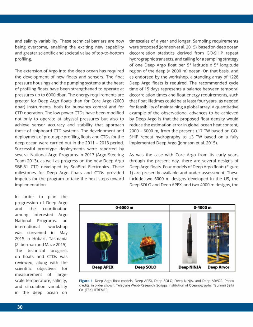
30

and salinity variability. These technical barriers are now being overcome, enabling the exciting new capability and greater scientific and societal value of top-to-bottom profiling.

The extension of Argo into the deep ocean has required the development of new floats and sensors. The float pressure housings and the pumping systems at the heart of profiling floats have been strengthened to operate at pressures up to 6000 dbar. The energy requirements are greater for Deep Argo floats than for Core Argo (2000 dbar) instruments, both for buoyancy control and for CTD operation. The low power CTDs have been modified not only to operate at abyssal pressures but also to achieve sensor accuracy and stability that approach those of shipboard CTD systems. The development and deployment of prototype profiling floats and CTDs for the deep ocean were carried out in the 2011 – 2013 period. Successful prototype deployments were reported by several National Argo Programs in 2013 (Argo Steering Team 2013), as well as progress on the new Deep Argo SBE-61 CTD developed by SeaBird Electronics. These milestones for Deep Argo floats and CTDs provided impetus for the program to take the next steps toward implementation.

In order to plan the progression of Deep Argo and the coordination among interested Argo National Programs, an international workshop was convened in May 2015 in Hobart, Tasmania (Zilberman and Maze 2015). The technical progress on floats and CTDs was reviewed, along with the scientific objectives for measurement of large-scale temperature, salinity, and circulation variability in the deep ocean on

timescales of a year and longer. Sampling requirements were proposed (Johnson et al. 2015), based on deep ocean decorrelation statistics derived from GO-SHIP repeat hydrographic transects, and calling for a sampling strategy of one Deep Argo float per 5° latitude x 5° longitude region of the deep (> 2000 m) ocean. On that basis, and as endorsed by the workshop, a standing array of 1228 Deep Argo floats is required. The recommended cycle time of 15 days represents a balance between temporal decorrelation times and float energy requirements, such that float lifetimes could be at least four years, as needed for feasibility of maintaining a global array. A quantitative example of the observational advances to be achieved by Deep Argo is that the proposed float density would reduce the estimation error in global ocean heat content, 2000 – 6000 m, from the present ±17 TW based on GO-SHIP repeat hydrography to ±3 TW based on a fully implemented Deep Argo (Johnson et al. 2015).

As was the case with Core Argo from its early years through the present day, there are several designs of Deep Argo floats. Four models of Deep Argo floats (Figure 1) are presently available and under assessment. These include two 6000 m designs developed in the US, the Deep SOLO and Deep APEX, and two 4000 m designs, the

Figure 1. Deep Argo float models: Deep APEX, Deep SOLO, Deep NINJA, and Deep ARVOR. Photo credits, in order shown: Teledyne Webb Research, Scripps Institution of Oceanography, Tsurumi Seiki Co. (TSK), IFREMER.

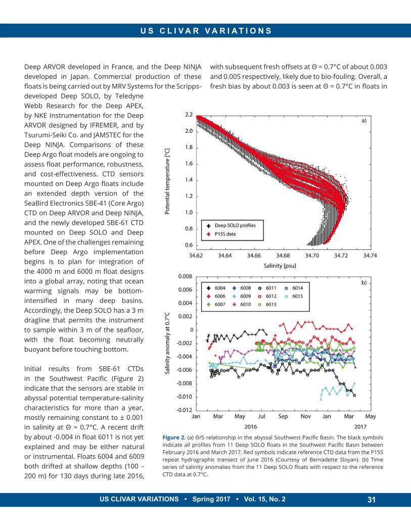
31

U S C L I V A R V A R I A T I O N S

US CLIVAR VARIATIONS • Spring 2017 • Vol. 15, No. 2 31

Deep ARVOR developed in France, and the Deep NINJA developed in Japan. Commercial production of these floats is being carried out by MRV Systems for the Scripps-developed Deep SOLO, by Teledyne Webb Research for the Deep APEX, by NKE Instrumentation for the Deep ARVOR designed by IFREMER, and by Tsurumi-Seiki Co. and JAMSTEC for the Deep NINJA. Comparisons of these Deep Argo float models are ongoing to assess float performance, robustness, and cost-effectiveness. CTD sensors mounted on Deep Argo floats include an extended depth version of the SeaBird Electronics SBE-41 (Core Argo) CTD on Deep ARVOR and Deep NINJA, and the newly developed SBE-61 CTD mounted on Deep SOLO and Deep APEX. One of the challenges remaining before Deep Argo implementation begins is to plan for integration of the 4000 m and 6000 m float designs into a global array, noting that ocean warming signals may be bottom-intensified in many deep basins. Accordingly, the Deep SOLO has a 3 m dragline that permits the instrument to sample within 3 m of the seafloor, with the float becoming neutrally buoyant before touching bottom.

Initial results from SBE-61 CTDs in the Southwest Pacific (Figure 2) indicate that the sensors are stable in abyssal potential temperature-salinity characteristics for more than a year, mostly remaining constant to ± 0.001 in salinity at Θ = 0.7°C. A recent drift by about -0.004 in float 6011 is not yet explained and may be either natural or instrumental. Floats 6004 and 6009 both drifted at shallow depths (100 – 200 m) for 130 days during late 2016,

with subsequent fresh offsets at Θ = 0.7°C of about 0.003 and 0.005 respectively, likely due to bio-fouling. Overall, a fresh bias by about 0.003 is seen at Θ = 0.7°C in floats in

Figure 2. (a) Θ/S relationship in the abyssal Southwest Pacific Basin. The black symbols indicate all profiles from 11 Deep SOLO floats in the Southwest Pacific Basin between February 2016 and March 2017. Red symbols indicate reference CTD data from the P15S repeat hydrographic transect of June 2016 (Courtesy of Bernadette Sloyan). (b) Time series of salinity anomalies from the 11 Deep SOLO floats with respect to the reference CTD data at 0.7°C.

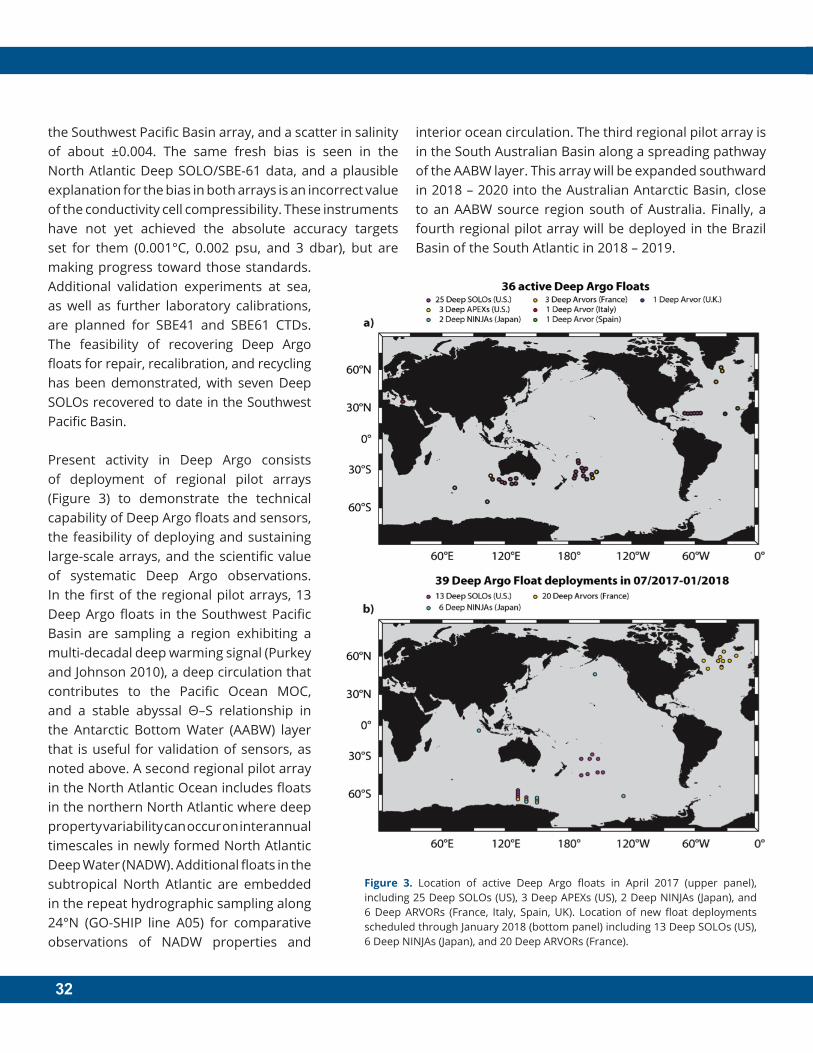
32

the Southwest Pacific Basin array, and a scatter in salinity of about ±0.004. The same fresh bias is seen in the North Atlantic Deep SOLO/SBE-61 data, and a plausible explanation for the bias in both arrays is an incorrect value of the conductivity cell compressibility. These instruments have not yet achieved the absolute accuracy targets set for them (0.001°C, 0.002 psu, and 3 dbar), but are making progress toward those standards. Additional validation experiments at sea, as well as further laboratory calibrations, are planned for SBE41 and SBE61 CTDs. The feasibility of recovering Deep Argo floats for repair, recalibration, and recycling has been demonstrated, with seven Deep SOLOs recovered to date in the Southwest Pacific Basin.

Present activity in Deep Argo consists of deployment of regional pilot arrays (Figure 3) to demonstrate the technical capability of Deep Argo floats and sensors, the feasibility of deploying and sustaining large-scale arrays, and the scientific value of systematic Deep Argo observations. In the first of the regional pilot arrays, 13 Deep Argo floats in the Southwest Pacific Basin are sampling a region exhibiting a multi-decadal deep warming signal (Purkey and Johnson 2010), a deep circulation that contributes to the Pacific Ocean MOC, and a stable abyssal Θ–S relationship in the Antarctic Bottom Water (AABW) layer that is useful for validation of sensors, as noted above. A second regional pilot array in the North Atlantic Ocean includes floats in the northern North Atlantic where deep property variability can occur on interannual timescales in newly formed North Atlantic Deep Water (NADW). Additional floats in the subtropical North Atlantic are embedded in the repeat hydrographic sampling along 24°N (GO-SHIP line A05) for comparative observations of NADW properties and

interior ocean circulation. The third regional pilot array is in the South Australian Basin along a spreading pathway of the AABW layer. This array will be expanded southward in 2018 – 2020 into the Australian Antarctic Basin, close to an AABW source region south of Australia. Finally, a fourth regional pilot array will be deployed in the Brazil Basin of the South Atlantic in 2018 – 2019.

Figure 3. Location of active Deep Argo floats in April 2017 (upper panel), including 25 Deep SOLOs (US), 3 Deep APEXs (US), 2 Deep NINJAs (Japan), and 6 Deep ARVORs (France, Italy, Spain, UK). Location of new float deployments scheduled through January 2018 (bottom panel) including 13 Deep SOLOs (US), 6 Deep NINJAs (Japan), and 20 Deep ARVORs (France) .

33

U S C L I V A R V A R I A T I O N S

US CLIVAR VARIATIONS • Spring 2017 • Vol. 15, No. 2 33

As of April 2017, there are 36 operational Deep Argo floats in all ocean basins, including 3 Deep APEX, 6 Deep ARVOR, 2 Deep NINJA, and 25 Deep SOLO (Figure 3a). An additional 39 deep float deployments are presently planned through January 2018 (Figure 3b). Following an assessment of multi-year float and sensor performance

in the regional Deep Argo pilot arrays, and contingent on increasing support levels from the international Argo partnership, the global implementation of the Deep Argo Program will begin. The era of systematic full-depth global ocean observations is coming.

References

Argo Steering Team, 2013: Report of the 14th Meeting of the International Argo Steering Team, Wellington, March 19 – 21, 2013. Available at http://www.argo.ucsd.edu/iast14.pdf.

Desbruyères, D. G., S. G. Purkey, E. L. McDonagh, G. C. Johnson, and B. A. King, 2016: Deep and abyssal ocean warming from 35 years of repeat hydrography. Geophys. Res. Lett., 43, 10356–10365, doi:10.1002/2016GL070413.

GCOS, 2016: The global observing system for climate: Implementation needs. GCOS Report 200, World Meteorological Organization, Geneva, 325 pp. Available at https://www.wmo.int/pages/prog/gcos/documents/IPComplete25July.pdf.

Johnson, G. C., J. M. Lyman, and S. G. Purkey, 2015: Informing deep Argo array design using Argo and full-depth hydrography section data. J. Atmos. Oceanic Technol., 32, 2187–2198, doi:10.1175/JTECH-D-15-0139.1.

Purkey, S. G., and G. C. Johnson, 2010: Warming of global abyssal and deep Southern Ocean waters between the 1990s and 2000s: Contributions to global heat and sea level rise budgets. J. Climate, 23, 6336–6350, doi:10.1175/2010JCLI3682.1.

Purkey, S. G., and G. C. Johnson, 2013: Antarctic Bottom Water warming and freshening: Contributions to sea level rise, ocean freshwater budgets, and global heat gain. J. Climate, 25, 6105–6122, doi:10.1175/jcli-d-12-00834.1.

Zilberman, N., and G. Maze, 2015: Report on the Deep Argo Implementation Workshop. Ifremer Doc. LPO-15-04, 36 pp. Available at http://archimer.ifremer.fr/doc/00281/39238/37799.pdf.

34

Deepgliders for observing ocean circulation and climate

Charles C. Eriksen

University of Washington

Mobile remotely controlled surveys of climatically important open ocean flows have become possible

through the development of autonomous underwater gliders capable of routinely profiling the entire water column. These vehicles, called Deepgliders, can operate to 6 km depth in missions with up to 10,000 km range at low speed (~0.25 m s-1). At higher speed (~0.5 m s-1), they can navigate across such powerful flows as the Gulf Stream with enough control to follow the ground track of an altimetry satellite, although their range is curtailed. Full-depth profiling enables estimation of absolute geostrophic current across sections, referenced to directly estimated depth averaged (i.e., barotropic) flow.

A recent pair of demonstration missions illustrated both the effectiveness and limitations of Deepglider sampling. A full-depth transect carried out from Bermuda to the New England Continental Slope demonstrated the feasibility of monitoring even the most energetic boundary flows autonomously with gliders, although with limited temporal resolution. The ~200 km width of major boundary currents implies that multiple vehicles would be required to collect roughly synoptic surveys (e.g., every 10 days). Full-depth repeat surveys of a 60 km by 60 km region surrounding the Bermuda Atlantic Time Series (BATS) site demonstrated the effectiveness of sampling regionally to resolve flows on eddy space and time scales.

Deepglider is the full-depth derivative of Seaglider, one of the three upper ocean gliders commonly in use

(Eriksen et al. 2001; Rudnick et al. 2004). It is designed to both measure full water column structure and to break the navigational limitations of upper ocean gliders in strong current conditions. Since currents are typically surface intensified, effective navigation requires higher vehicle speed for upper ocean vehicles than would be required if a glider could dive deeper. Higher speed dramatically raises energy consumption, reducing range and endurance proportionately. While upper ocean gliders have proven adept at sampling the relatively modest flows of eastern boundary current systems, they are much less controllable in the more energetic environments of western boundary regions and high geostrophic eddy activity. The Office of Naval Research Ocean Engineering and Marine Systems Program has supported most of Deepglider development, while the National Science Foundation Physical Oceanography Program has supported final stages of this process and transition to scientific applications.

The initial Deepglider prototype mimicked the tapered Seaglider shape, but fabrication of a tapered hull with tapering wall thickness proved beyond state of the art carbon fiber manufacturing capability. Carbon fiber was selected as the hull material because of it high strength to weight ratio (about seven times that of titanium), durability to pressure cycling, and well-developed fabrication technology. Built at the Boeing Development Center in Tukwila, Washington, and designed in consultation with engineers there, a tapered hull could not attain the desired pressure rating. It was abandoned in favor of

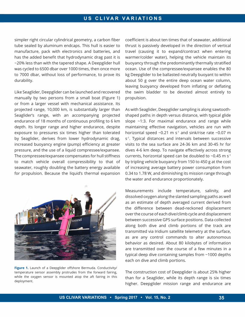
35

U S C L I V A R V A R I A T I O N S

US CLIVAR VARIATIONS • Spring 2017 • Vol. 15, No. 2 35

simpler right circular cylindrical geometry, a carbon fiber tube sealed by aluminum endcaps. This hull is easier to manufacture, pack with electronics and batteries, and has the added benefit that hydrodynamic drag past it is ~20% less than with the tapered shape. A Deepglider hull was cycled to 6500 dbar over 1000 times, then once more to 7000 dbar, without loss of performance, to prove its durability.

Like Seaglider, Deepglider can be launched and recovered manually by two persons from a small boat (Figure 1) or from a larger vessel with mechanical assistance. Its projected range, 10,000 km, is substantially larger than Seaglider’s range, with an accompanying projected endurance of 18 months of continuous profiling to 6 km depth. Its longer range and higher endurance, despite exposure to pressures six times higher than tolerated by Seaglider, derives from lower hydrodynamic drag, increased buoyancy engine (pump) efficiency at greater pressure, and the use of a liquid compressee/expansee. The compressee/expansee compensates for hull stiffness to match vehicle overall compressibility to that of seawater, roughly doubling the battery energy available for propulsion. Because the liquid’s thermal expansion

coefficient is about ten times that of seawater, additional thrust is passively developed in the direction of vertical travel (causing it to expand/contract when entering warmer/colder water), helping the vehicle maintain its buoyancy through the predominantly thermally stratified ocean. Use of the compressee/expansee enables the 80 kg Deepglider to be ballasted neutrally buoyant to within about 50 g over the entire deep ocean water column, leaving buoyancy developed from inflating or deflating the swim bladder to be devoted almost entirely to propulsion.

As with Seaglider, Deepglider sampling is along sawtooth-shaped paths in depth versus distance, with typical glide slope ~1:3. For maximal endurance and range while maintaining effective navigation, vehicles are run with horizontal speed ~0.21 m s-1 and sink/rise rate ~0.07 m s-1. Typical distances and intervals between successive visits to the sea surface are 24-36 km and 30-45 hr for dives 4-6 km deep. To navigate effectively across strong currents, horizontal speed can be doubled to ~0.45 m s-1 by tripling vehicle buoyancy from 150 to 450 g at the cost of increasing average battery power consumption from 0.34 to 1.78 W, and diminishing its mission range through the water and endurance proportionately.

Measurements include temperature, salinity, and dissolved oxygen along the slanted sampling paths as well as an estimate of depth averaged current derived from the difference between dead-reckoned displacement over the course of each dive/climb cycle and displacement between successive GPS surface positions. Data collected along both dive and climb portions of the track are transmitted via Iridium satellite telemetry at the surface, as are any control commands to alter autonomous behavior as desired. About 80 kilobytes of information are transmitted over the course of a few minutes in a typical deep dive containing samples from ~1000 depths each on dive and climb portions.

The construction cost of Deepglider is about 25% higher than for a Seaglider, while its depth range is six times higher. Deepglider mission range and endurance are

Figure 1. Launch of a Deepglider offshore Bermuda. Conductivity/temperature sensor assembly protrudes from the forward fairing, while the oxygen sensor is mounted atop the aft fairing in this deployment.

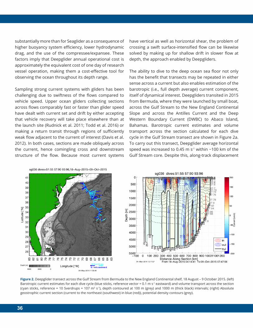
36

substantially more than for Seaglider as a consequence of higher buoyancy system efficiency, lower hydrodynamic drag, and the use of the compressee/expansee. These factors imply that Deepglider annual operational cost is approximately the equivalent cost of one day of research vessel operation, making them a cost-effective tool for observing the ocean throughout its depth range.

Sampling strong current systems with gliders has been challenging due to swiftness of the flows compared to vehicle speed. Upper ocean gliders collecting sections across flows comparably fast or faster than glider speed have dealt with current set and drift by either accepting that vehicle recovery will take place elsewhere than at the launch site (Rudnick et al. 2011; Todd et al. 2016) or making a return transit through regions of sufficiently weak flow adjacent to the current of interest (Davis et al. 2012). In both cases, sections are made obliquely across the current, hence comingling cross and downstream structure of the flow. Because most current systems

have vertical as well as horizontal shear, the problem of crossing a swift surface-intensified flow can be likewise solved by making up for shallow drift in slower flow at depth, the approach enabled by Deepgliders.

The ability to dive to the deep ocean sea floor not only has the benefit that transects may be repeated in either sense across a current but also enables estimation of the barotropic (i.e., full depth average) current component, itself of dynamical interest. Deepgliders transited in 2015 from Bermuda, where they were launched by small boat, across the Gulf Stream to the New England Continental Slope and across the Antilles Current and the Deep Western Boundary Current (DWBC) to Abaco Island, Bahamas. Barotropic current estimates and volume transport across the section calculated for each dive cycle in the Gulf Stream transect are shown in Figure 2a. To carry out this transect, Deepglider average horizontal speed was increased to 0.45 m s-1 within ~100 km of the Gulf Stream core. Despite this, along-track displacement

Figure 2. Deepglider transect across the Gulf Stream from Bermuda to the New England Continental shelf, 18 August – 9 October 2015. (left) Barotropic current estimates for each dive cycle (blue sticks, reference vector = 0.1 m s-1 eastward) and volume transport across the section (cyan sticks, reference = 10 Sverdrups = 107 m3 s-1), depth contoured at 100 m (grey) and 1000 m (thick black) intervals; (right) Absolute geostrophic current section (current to the northeast (southwest) in blue (red)), potential density contours (grey).

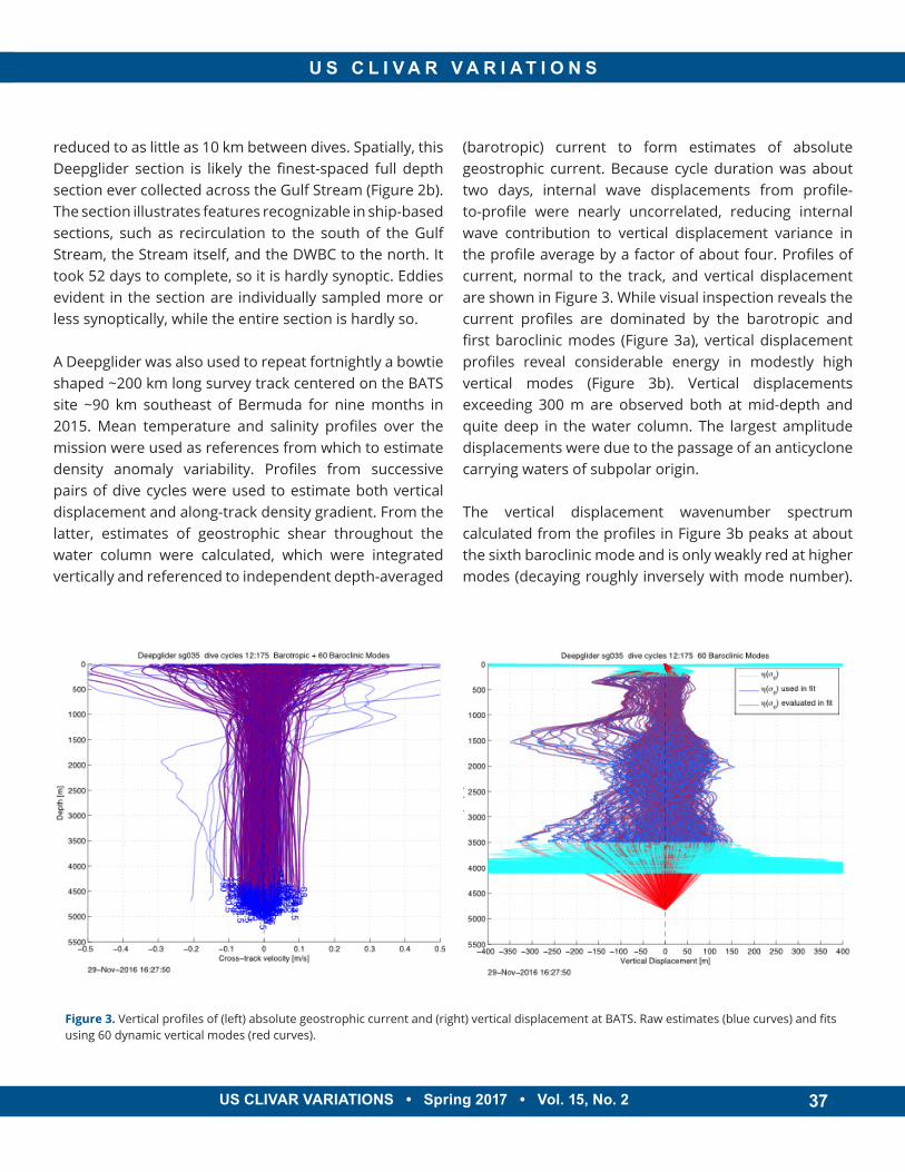
37

U S C L I V A R V A R I A T I O N S

US CLIVAR VARIATIONS • Spring 2017 • Vol. 15, No. 2 37

reduced to as little as 10 km between dives. Spatially, this Deepglider section is likely the finest-spaced full depth section ever collected across the Gulf Stream (Figure 2b). The section illustrates features recognizable in ship-based sections, such as recirculation to the south of the Gulf Stream, the Stream itself, and the DWBC to the north. It took 52 days to complete, so it is hardly synoptic. Eddies evident in the section are individually sampled more or less synoptically, while the entire section is hardly so.

A Deepglider was also used to repeat fortnightly a bowtie shaped ~200 km long survey track centered on the BATS site ~90 km southeast of Bermuda for nine months in 2015. Mean temperature and salinity profiles over the mission were used as references from which to estimate density anomaly variability. Profiles from successive pairs of dive cycles were used to estimate both vertical displacement and along-track density gradient. From the latter, estimates of geostrophic shear throughout the water column were calculated, which were integrated vertically and referenced to independent depth-averaged

(barotropic) current to form estimates of absolute geostrophic current. Because cycle duration was about two days, internal wave displacements from profile-to-profile were nearly uncorrelated, reducing internal wave contribution to vertical displacement variance in the profile average by a factor of about four. Profiles of current, normal to the track, and vertical displacement are shown in Figure 3. While visual inspection reveals the current profiles are dominated by the barotropic and first baroclinic modes (Figure 3a), vertical displacement profiles reveal considerable energy in modestly high vertical modes (Figure 3b). Vertical displacements exceeding 300 m are observed both at mid-depth and quite deep in the water column. The largest amplitude displacements were due to the passage of an anticyclone carrying waters of subpolar origin.

The vertical displacement wavenumber spectrum calculated from the profiles in Figure 3b peaks at about the sixth baroclinic mode and is only weakly red at higher modes (decaying roughly inversely with mode number).

Figure 3. Vertical profiles of (left) absolute geostrophic current and (right) vertical displacement at BATS. Raw estimates (blue curves) and fits using 60 dynamic vertical modes (red curves).

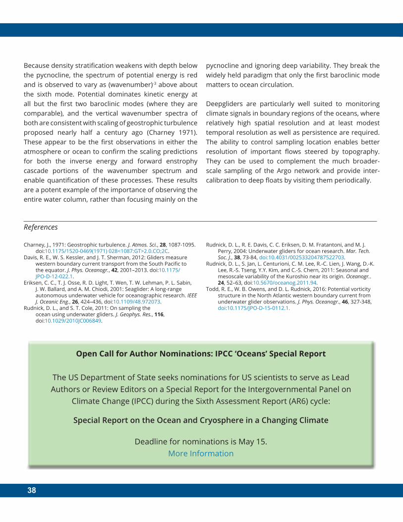
38

Because density stratification weakens with depth below the pycnocline, the spectrum of potential energy is red and is observed to vary as (wavenumber)-3 above about the sixth mode. Potential dominates kinetic energy at all but the first two baroclinic modes (where they are comparable), and the vertical wavenumber spectra of both are consistent with scaling of geostrophic turbulence proposed nearly half a century ago (Charney 1971). These appear to be the first observations in either the atmosphere or ocean to confirm the scaling predictions for both the inverse energy and forward enstrophy cascade portions of the wavenumber spectrum and enable quantification of these processes. These results are a potent example of the importance of observing the entire water column, rather than focusing mainly on the

pycnocline and ignoring deep variability. They break the widely held paradigm that only the first baroclinic mode matters to ocean circulation.

Deepgliders are particularly well suited to monitoring climate signals in boundary regions of the oceans, where relatively high spatial resolution and at least modest temporal resolution as well as persistence are required. The ability to control sampling location enables better resolution of important flows steered by topography. They can be used to complement the much broader-scale sampling of the Argo network and provide inter-calibration to deep floats by visiting them periodically.

References

Charney, J., 1971: Geostrophic turbulence. J. Atmos. Sci., 28, 1087-1095. doi:10.1175/1520-0469(1971) 028<1087:GT>2.0.CO;2C.

Davis, R. E., W. S. Kessler, and J. T. Sherman, 2012: Gliders measure western boundary current transport from the South Pacific to the equator. J. Phys. Oceanogr., 42, 2001–2013. doi:10.1175/JPO-D-12-022.1.

Eriksen, C. C., T. J. Osse, R. D. Light, T. Wen, T. W. Lehman, P. L. Sabin, J. W. Ballard, and A. M. Chiodi, 2001: Seaglider: A long-range autonomous underwater vehicle for oceanographic research. IEEE J. Oceanic Eng., 26, 424–436, doi:10.1109/48.972073.

Rudnick, D. L., and S. T. Cole, 2011: On sampling the ocean using underwater gliders. J. Geophys. Res., 116, doi:10.1029/2010JC006849.

Rudnick, D. L., R. E. Davis, C. C. Eriksen, D. M. Fratantoni, and M. J. Perry, 2004: Underwater gliders for ocean research. Mar. Tech. Soc. J., 38, 73-84, doi:10.4031/002533204787522703.

Rudnick, D. L., S. Jan, L. Centurioni, C. M. Lee, R.-C. Lien, J. Wang, D.-K. Lee, R.-S. Tseng, Y.Y. Kim, and C.-S. Chern, 2011: Seasonal and mesoscale variability of the Kuroshio near its origin. Oceanogr.. 24, 52–63, doi:10.5670/oceanog.2011.94.

Todd, R. E., W. B. Owens, and D. L. Rudnick, 2016: Potential vorticity structure in the North Atlantic western boundary current from underwater glider observations. J. Phys. Oceanogr., 46, 327-348, doi:10.1175/JPO-D-15-0112.1.

Open Call for Author Nominations: IPCC ‘Oceans’ Special Report

The US Department of State seeks nominations for US scientists to serve as Lead Authors or Review Editors on a Special Report for the Intergovernmental Panel on

Climate Change (IPCC) during the Sixth Assessment Report (AR6) cycle:

Special Report on the Ocean and Cryosphere in a Changing Climate

Deadline for nominations is May 15. More Information

39

U S C L I V A R V A R I A T I O N S

US CLIVAR VARIATIONS • Spring 2017 • Vol. 15, No. 2 39

ANNOUNCEMENTS

US Climate Variability and Predictability(CLIVAR) Program

1201 New York Ave. NW, Suite 400Washington, DC 20005

(202) 787-1682

US CLIVARClimate Variability & Predictabilit

y

US CLIVAR acknowledges support from these US agencies:

This material was developed with federal support of NASA, NSF, and DOE (AGS-1502208), and NOAA (NA11OAR4310213).

Any opinions, findings, conclusions, or recommendations expressed in this material are those of the authors and do not necessarily reflect the views of the sponsoring agencies.

www.usclivar.orguscpo@usclivar.orgtwitter.com/usclivar

CLICK HERE TO JOIN!

Tuesday, May 1612:00 - 1:30 PM ET

Featuring authors from this edition:Gregory Johnson, NOAA Pacific Marine Environmental Laboratory

Lynne Talley, Scripps Institution of Oceanography Felix Landerer, NASA Jet Propulsion Laboratory

Nathalie Zilberman, Scripps Institution of Oceanography Charlie Eriksen, University of Washington

Variations Webinar Series

A case for observing the deep ocean