Topic 4 Electronic Structure Lecture 1

Variational Methods for Electronic Structure

The hydrogen atom is a two-body system consisting of a proton and an electron. If spin and relativistic

effects are ignored, then the Schrodinger equation for the hydrogen atom can be solved exactly. In this

respect, it is similar to the Kepler problem in classical mechanics.

The classical three-body problem is nonintegrable and exact solutions exist only in very special cases. The

analogous quantum mechanical system is the Helium atom, which consists of a nucleus and two electrons.

This quantum mechanical problem cannot be solved exactly even if spin and relativisitic effects are ignored.

The following table from the review article Rev. Mod. Phys. 72, 497-544 (2000) by Tanner et al.

PHY 411-506 Computational Physics 2 1 Monday, March 10

Topic 4 Electronic Structure Lecture 1

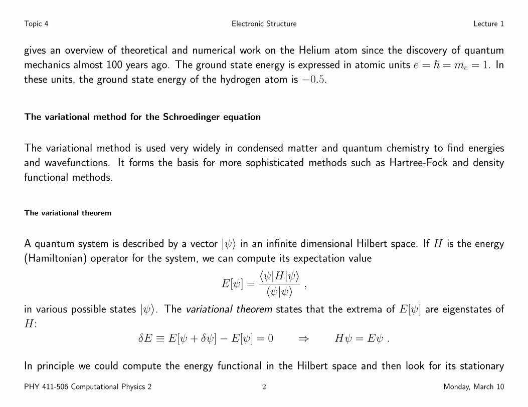
gives an overview of theoretical and numerical work on the Helium atom since the discovery of quantum

mechanics almost 100 years ago. The ground state energy is expressed in atomic units e = ~ = me = 1. In

these units, the ground state energy of the hydrogen atom is −0.5.

The variational method for the Schroedinger equation

The variational method is used very widely in condensed matter and quantum chemistry to find energies

and wavefunctions. It forms the basis for more sophisticated methods such as Hartree-Fock and density

functional methods.

The variational theorem

A quantum system is described by a vector |ψ〉 in an infinite dimensional Hilbert space. If H is the energy

(Hamiltonian) operator for the system, we can compute its expectation value

E[ψ] =〈ψ|H|ψ〉〈ψ|ψ〉

,

in various possible states |ψ〉. The variational theorem states that the extrema of E[ψ] are eigenstates of

H:

δE ≡ E[ψ + δψ]− E[ψ] = 0 ⇒ Hψ = Eψ .

In principle we could compute the energy functional in the Hilbert space and then look for its stationary

PHY 411-506 Computational Physics 2 2 Monday, March 10

Topic 4 Electronic Structure Lecture 1

points: these would give us the eigen energies and eigenvectors. This is not practical however because the

space is infinite dimensional! It is hard enough to find a stationary point in a one-dimensional space!

The variational method looks for stationary points in a finite dimensional subspace of the Hilbert space.

Suppose this subspace in N -dimensional. If |χp〉, p = 1, . . . , N is a set of orthonormal basis vectors, i.e.,

unit vectors

〈χp|χq〉 = δpq ,

then H can be represented by an N ×N matrix H with elements

Hpq = 〈χp|H|χq〉 , p, q = 1, . . . , N .

We are looking for stationary states

ψ =

N∑p=1

Cp|χp〉 ,

where Cp are complex coefficients to be determined. The stationary condition becomes a matrix eigenvalue

equation:

HC = EC ,

N∑q=1

HpqCq = ECp , p = 1, . . . , N .

Let’s recall some results from quantum mechanics:

� H is Hermitian H† = H, i.e., Hpq = H∗qp. Actually in the problems we will consider, H is a real

symmetric matrix.

PHY 411-506 Computational Physics 2 3 Monday, March 10

Topic 4 Electronic Structure Lecture 1

� There are exactly N real eigenvalues.

� The N eigenvectors corresponding to these eigenvalues span the subspace and can be chosen to be

orthonormal.

The generalized eigenvalue problem

It is actually not necessary to choose an orthonormal basis set |χp〉. Any linearly independent set of basis

vectors can be used as we will see in the examples. The eigenvalue equation for a generalized basis set is

HC = ESC ,

N∑q=1

HpqCq = E

N∑q=1

SpqCq , p = 1, . . . , N .

where the overlap matrix S has elements

Spq = 〈χp|χq〉 .

It can be shown that

� S is Hermitian, and

� The eigenvalues of S are real and positive definite, i.e., > 0.

These properties can be used to convert the generalized eigenvalue problem to an eigenvalue problem with

an orthonormal basis.

PHY 411-506 Computational Physics 2 4 Monday, March 10

Topic 4 Electronic Structure Lecture 1

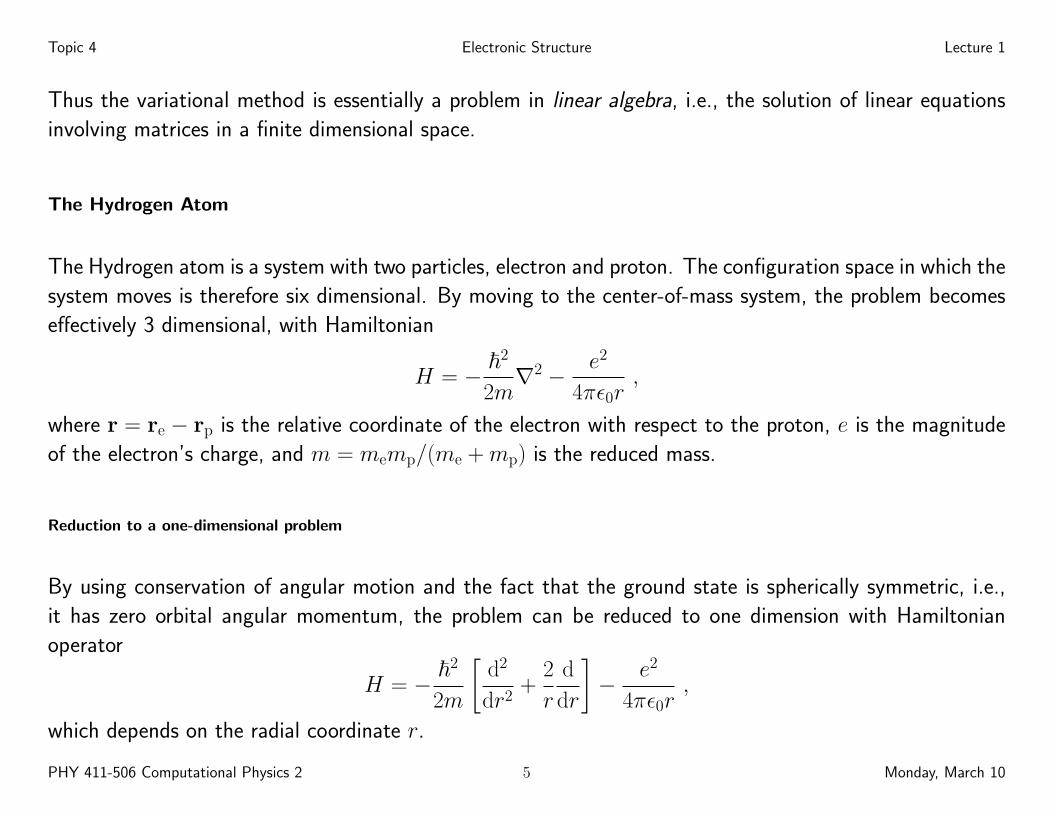
Thus the variational method is essentially a problem in linear algebra, i.e., the solution of linear equations

involving matrices in a finite dimensional space.

The Hydrogen Atom

The Hydrogen atom is a system with two particles, electron and proton. The configuration space in which the

system moves is therefore six dimensional. By moving to the center-of-mass system, the problem becomes

effectively 3 dimensional, with Hamiltonian

H = − ~2

2m∇2 − e2

4πε0r,

where r = re − rp is the relative coordinate of the electron with respect to the proton, e is the magnitude

of the electron’s charge, and m = memp/(me + mp) is the reduced mass.

Reduction to a one-dimensional problem

By using conservation of angular motion and the fact that the ground state is spherically symmetric, i.e.,

it has zero orbital angular momentum, the problem can be reduced to one dimension with Hamiltonian

operator

H = − ~2

2m

[d2

dr2+

2

r

d

dr

]− e2

4πε0r,

which depends on the radial coordinate r.

PHY 411-506 Computational Physics 2 5 Monday, March 10

Topic 4 Electronic Structure Lecture 1

Exact solution for the ground state

The exact ground state energy and wavefunction are given by

E0 = − e2

2a0, ψ0(r) ∼ e−r/a0 .

where the Bohr radius

a0 =4πε0~2

me2.

It is convenient to use atomic units in which ~ = m = e2/(4πε0) = 1 so

H = −1

2

[d2

dr2+

2

r

d

dr

]− 1

r, E0 = −1

2, ψ0(r) ∼ e−r .

Simple variational trial wave function

A simple trial wave function for the Hydrogen atom ground state is

ψT,α(r) = e−αr .

The Hamiltonian acting on this function gives:

HψT,α(r) =

[−~2α2

2m+

(~2α

m− e2

4πε0

)1

r

]ψT,α(r) ≡ E(r)ψT,α(r) .

PHY 411-506 Computational Physics 2 6 Monday, March 10

Topic 4 Electronic Structure Lecture 1

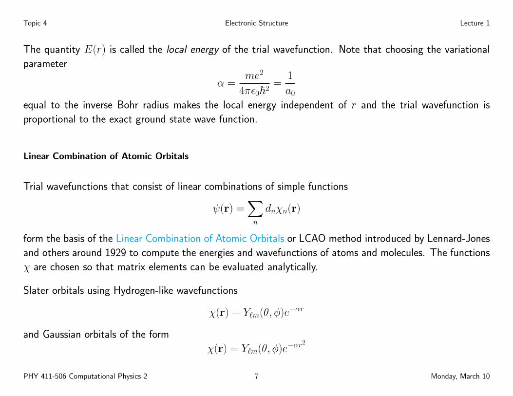
The quantity E(r) is called the local energy of the trial wavefunction. Note that choosing the variational

parameter

α =me2

4πε0~2=

1

a0

equal to the inverse Bohr radius makes the local energy independent of r and the trial wavefunction is

proportional to the exact ground state wave function.

Linear Combination of Atomic Orbitals

Trial wavefunctions that consist of linear combinations of simple functions

ψ(r) =∑n

dnχn(r)

form the basis of the Linear Combination of Atomic Orbitals or LCAO method introduced by Lennard-Jones

and others around 1929 to compute the energies and wavefunctions of atoms and molecules. The functions

χ are chosen so that matrix elements can be evaluated analytically.

Slater orbitals using Hydrogen-like wavefunctions

χ(r) = Y`m(θ, φ)e−αr

and Gaussian orbitals of the form

χ(r) = Y`m(θ, φ)e−αr2

PHY 411-506 Computational Physics 2 7 Monday, March 10

Topic 4 Electronic Structure Lecture 1

are the most widely used forms. Gaussian orbitals form the basis of many quantum chemistry computer

codes.

Because Slater orbitals give exact results for Hydrogen, we will use Gaussian orbitals to test the LCAO

method on Hydrogen, following S.F. Boys, Proc. Roy. Soc. A 200, 542 (1950) and W.R. Ditchfield, W.J.

Hehre and J.A. Pople, J. Chem. Phys. Rev. 52, 5001 (1970) with the basis set

ψ(r) =

N−1∑i=0

digs(αi, r) ,

where

gs(α, r) =

(2α

π

)34

e−αr2

for the ` = 0 s-wave states.

Because products of Gaussians are also Gaussian, the required matrix elements are easily computed:

Sij =

∫d3r e−αir

2e−αir

2=

(π

αi + αj

)3/2

,

Tij = − ~2

2m

∫d3r e−αir

2∇2e−αjr2

=3~2

m

αiαjπ3/2

(αi + αj)5/2,

Vij = −e2

∫d3r e−αir

2 1

re−αjr

2= − 2πe2

αi + αj.

PHY 411-506 Computational Physics 2 8 Monday, March 10

Topic 4 Electronic Structure Lecture 1

The 1998 Nobel Prize in Chemistry was divided equally between Walter Kohn ”for his development of the

density-functional theory” and John A. Pople ”for his development of computational methods in quantum

chemistry”.

LCAO Codes for Hydrogen

The BFGS method can be used to minimize the variational energy.

hydrogen.py

from math import exp, pi, sqrt

from tools.linalg import minimize_BFGS

# physical constants

hbar = 1.0 # Planck’s constant / 2pi

m = 1.0 # electron mass

e = 1.0 # proton charge

# LCAO variational wave function

# psi = sum( d_i g(alpha_i, r) ) for i = 0, 1, 2, ...

# assume d_0 = 1 and vary alpha_0, d_1, alpha_1, d_2, alpha_2, ...

# vector of variational parameters

PHY 411-506 Computational Physics 2 9 Monday, March 10

Topic 4 Electronic Structure Lecture 1

p = [ 1.0, 1.0, 0.5 ] # initial guess for [ alpha_0, d_1, alpha_1 ]

N = int( (len(p) + 1) / 2 ) # number of Gaussians

accuracy = 1.0e-6 # desired accuracy for numerical operations

def g(alpha, r): # normalized s-wave Gaussian orbital

return (2.0 * alpha / pi)**(3.0/4.0) * exp(-alpha * r**2)

def Sij(alpha_i, alpha_j): # matrix elements of S

return (pi / (alpha_i + alpha_j))**(3.0/2.0)

def Tij(alpha_i, alpha_j): # matrix elements of T

return (3.0 * hbar**2 / m * alpha_i * alpha_j *

pi**(3.0/2.0) / (alpha_i + alpha_j)**(5.0/2.0))

def Vij(alpha_i, alpha_j): # matrix elements of V

return - 2.0 * e**2 * pi / (alpha_i + alpha_j)

def E(alpha, d): # energy as function of N alpha_i and d_i

S = H = 0.0

for i in range(len(alpha)):

for j in range(len(alpha)):

PHY 411-506 Computational Physics 2 10 Monday, March 10

Topic 4 Electronic Structure Lecture 1

fac = (alpha[i] * alpha[j])**(3.0/4.0)* d[i] * d[j]

H += fac * (Tij(alpha[i], alpha[j]) + Vij(alpha[i], alpha[j]))

S += fac * Sij(alpha[i], alpha[j])

return H / S

def func(p): # function for BFGS minimization

# assume p = [ alpha_0, d_1, alpha_1, d_2, alpha_2, ... ]

alpha = [ max(p[2 * i], accuracy) for i in range(N) ]

d = [ 1.0 ]

d.extend(p[2 * i + 1] for i in range(N - 1))

return E(alpha, d)

def dfunc(p, g): # gradient of func for BFGS minimization

# use symmetric finite difference f’(x) = (f(x+eps) - f(x-eps)) / (2 eps)

eps = 0.5 * accuracy # finite difference

for i in range(len(p)):

p1 = list(p)

p1[i] += eps

p2 = list(p)

p2[i] -= eps

g[i] = (func(p1) - func(p2)) / (2 * eps)

return

PHY 411-506 Computational Physics 2 11 Monday, March 10

Topic 4 Electronic Structure Lecture 1

def norm(p): # norm of LCAO

alpha = [ p[2 * i] for i in range(N) ]

d = [ 1.0 ]

d.extend(p[2 * i + 1] for i in range(N - 1))

norm = 0.0

for i in range(N):

for j in range(N):

norm += Sij(alpha[i], alpha[j]) * d[i] * d[j]

return sqrt(norm)

print(" Variational method for Hydrogen using Gaussian LCAO")

print(" Minimize <psi|H|psi>/<psi|psi> using BFGS algorithm")

gtol = accuracy

iterations, e = minimize_BFGS(p, gtol, func, dfunc)

print(" number of Gaussians N = " + repr(N))

print(" number of iterations = " + repr(iterations))

print(" energy E = " + repr(e))

print(" i\talpha_i\t\t\td_i")

exit

for i in range(N):

alpha_i = p[2 * i]

PHY 411-506 Computational Physics 2 12 Monday, March 10

Topic 4 Electronic Structure Lecture 1

if i == 0:

d_i = 1.0 / norm(p)

else:

d_i = p[2 * i - 1] / norm(p)

print(" " + repr(i) + "\t" + repr(p[2*i]) + "\t" + repr(d_i))

The Helium Atom

The Helium atom is a 3-particle problem: two electrons orbit around a nucleus, which consists of two protons

with charge e each and two neutral neutrons. The nucleus, which is ∼ 8, 000 times more massive than an

electron, can be assumed to be at rest at the origin of the coordinate system. The electrons have positions

r1 and r2. This is simpler than making a transformation to the center-of-mass system of the three particles,

and it is sufficiently accurate.

If we use atomic units with ~ = me = e = 1, the Hamiltonian for the motion of the two electrons can be

written

H = −1

2∇2

1 −1

2∇2

2 −2

r1− 2

r2+

1

r12,

where

r12 = |r12| = |r1 − r2| .The terms −2/ri represent the negative (attractive) potential energy between each electron with charge −1

and the Helium nucleus with charge +2, and the term +1/r12 represents the positive (repulsive) potential

PHY 411-506 Computational Physics 2 13 Monday, March 10

Topic 4 Electronic Structure Lecture 1

energy between the two electrons.

A simple choice of variational trial wave function

If the repulsive term 1/r12 were not present, then the Hamiltonian would be that of two independent

Hydrogen-like atoms. It can be shown that the energy and ground state wave function of a Hydrogen-like

atom whose nucleus has charge Z are given by

E0 = −Z2

2, ψ0 ∼ e−Zr .

The wave function of the combined atom with two non-interacting electrons would be the product of two

such wave functions:

ψ(r1, r2) ∼ e−2r1e−2r2 .

This suggests a trial wave function of the form

ΨT,α = e−αr1e−αr2 ,

similar to what was done for the Hydrogen atom. If the electron-electron interaction is neglected, then the

average energy with this wave function can be calculated⟨−1

2∇2

1 −1

2∇2

2 −2

r1− 2

r2

⟩= 2× α2

2− 2× 2× α ,

PHY 411-506 Computational Physics 2 14 Monday, March 10

Topic 4 Electronic Structure Lecture 1

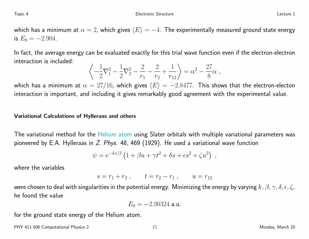
which has a minimum at α = 2, which gives 〈E〉 = −4. The experimentally measured ground state energy

is E0 = −2.904.

In fact, the average energy can be evaluated exactly for this trial wave function even if the electron-electron

interaction is included: ⟨−1

2∇2

1 −1

2∇2

2 −2

r1− 2

r2+

1

r12

⟩= α2 − 27

8α ,

which has a minimum at α = 27/16, which gives 〈E〉 = −2.8477. This shows that the electron-electon

interaction is important, and including it gives remarkably good agreement with the experimental value.

Variational Calculations of Hylleraas and others

The variational method for the Helium atom using Slater orbitals with multiple variational parameters was

pioneered by E.A. Hylleraas in Z. Phys. 48, 469 (1929). He used a variational wave function

ψ = e−ks/2(1 + βu + γt2 + δs + εs2 + ζu2

),

where the variables

s = r1 + r2 , t = r2 − r1 , u = r12

were chosen to deal with singularities in the potential energy. Minimizing the energy by varying k, β, γ, δ, ε, ζ,

he found the value

E0 = −2.90324 a.u.

for the ground state energy of the Helium atom.

PHY 411-506 Computational Physics 2 15 Monday, March 10

Topic 4 Electronic Structure Lecture 1

Chandrasekhar, Elbert and Herzberg Phys. Rev. 91, 1172 (1953) improved on Hylleraas’ calculation by

using 9 parameters

e−ks/2(1 + βu + γt2 + δs + εs2 + ζu2 + χ6su + χ7t

2u + χ8u3 + χ9t

2u2)

and found

E0 = −2.903603 a.u.

Numerous other variational calculations have since been performed, one of the most recent being by V.I.

Korobov Phys. Rev. A 66, 024501 (2002) who used 5200 variational parameters and obtained

E0 = −2.903724377034119598311159 a.u.

The review article by G.W.F. Drake, Physica Scripta, T83, 83 (1999) summarizes experimental and theo-

retical work on the Helium atom since the early calculations of Hylleraas.

Evaluation of Matrix Elements

The expectation value of the energy in the variational state can be evaluated analytically using formulas in

Wikipedia: Slater type orbital.

PHY 411-506 Computational Physics 2 16 Monday, March 10