Variational Graph Recurrent Neural Networks

Ehsan Hajiramezanali†∗, Arman Hasanzadeh†∗, Nick Duffield†, Krishna Narayanan†,Mingyuan Zhou‡, Xiaoning Qian†

† Department of Electrical and Computer Engineering, Texas A&M University{ehsanr, armanihm, duffieldng, krn, xqian}@tamu.edu‡McCombs School of Business, The University of Texas at Austin

mingyuan.zhou@mccombs.utexas.edu

Abstract

Representation learning over graph structured data has been mostly studied in staticgraph settings while efforts for modeling dynamic graphs are still scant. In thispaper, we develop a novel hierarchical variational model that introduces additionallatent random variables to jointly model the hidden states of a graph recurrentneural network (GRNN) to capture both topology and node attribute changes indynamic graphs. We argue that the use of high-level latent random variables inthis variational GRNN (VGRNN) can better capture potential variability observedin dynamic graphs as well as the uncertainty of node latent representation. Withsemi-implicit variational inference developed for this new VGRNN architecture (SI-VGRNN), we show that flexible non-Gaussian latent representations can furtherhelp dynamic graph analytic tasks. Our experiments with multiple real-worlddynamic graph datasets demonstrate that SI-VGRNN and VGRNN consistentlyoutperform the existing baseline and state-of-the-art methods by a significantmargin in dynamic link prediction.

1 Introduction

Node embedding maps each node in a graph to a vector in a low-dimensional latent space, in whichclassical feature vector-based machine learning formulations can be adopted [5]. Most of the existingnode embedding techniques assume that the graph is static and that learning tasks are performedon fixed sets of nodes and edges [19, 23, 12, 20, 14, 1]. However, many real-world problems aremodeled by dynamic graphs, where graphs are constantly evolving over time. Such graphs have beentypically observed in social networks, citation networks, and financial transaction networks. A naivesolution to node embedding for dynamic graphs is simply applying static methods to each snapshot ofdynamic graphs. Among many potential problems of such a naive solution, it is clear that it ignoresthe temporal dependencies between snapshots.

Several node embedding methods have been proposed to capture the temporal graph evolution forboth networks without attributes [10, 26] and attributed networks [24, 16]. However, all of theexisting dynamic graph embedding approaches represent each node by a deterministic vector ina low-dimensional space [2]. Such deterministic representations lack the capability of modelinguncertainty of node embedding, which is a natural consideration when having multiple informationsources, i.e. node attributes and graph structure.

In this paper, we propose a novel node embedding method for dynamic graphs that maps each node toa random vector in the latent space. More specifically, we first introduce a dynamic graph autoencodermodel, namely graph recurrent neural network (GRNN), by extending the use of graph convolutional

∗Both authors contributed equally.

33rd Conference on Neural Information Processing Systems (NeurIPS 2019), Vancouver, Canada.

neural networks (GCRN) [21] to dynamic graphs. Then, we argue that GRNN lacks the expressivepower for fully capturing the complex dependencies between topological evolution and time-varyingnode attributes because the output probability in standard RNNs is limited to either a simple unimodaldistribution or a mixture of unimodal distributions [3, 22, 6, 8]. Next, to increase the expressivepower of GRNN in addition to modeling the uncertainty of node latent representations, we proposevariational graph recurrent neural network (VGRNN) by adopting high-level latent random variablesin GRNN. Our proposed VGRNN is capable of learning interpretable latent representation as well asbetter modeling of very sparse dynamic graphs.

To further boost the expressive power and interpretability of our new VGRNN method, we integratesemi-implicit variational inference [25] with VGRNN. We show that semi-implicit variational graphrecurrent neural network (SI-VGRNN) is capable of inferring more flexible and complex posteriors.Our experiments demonstrate the superior performance of VGRNN and SI-VGRNN in dynamic linkprediction tasks in several real-world dynamic graph datasets compared to baseline and state-of-the-artmethods.

2 Background

Graph convolutional recurrent networks (GCRN). GCRN was introduced by Seo et al. [21]to model time series data defined over nodes of a static graph. Series of frames in videos andspatio-temporal measurements on a network of sensors are two examples of such datasets. GCRNcombines graph convolutional networks (GCN) [4] with recurrent neural networks (RNN) to capturespatial and temporal patterns in data. More precisely, given a graph G with N nodes, whosetopology is determined by the adjacency matrix A ∈ RN×N , and a sequence of node attributesX = {X(1),X(2), . . . ,X(T )}, GCRN reads M -dimensional node attributes X(t) ∈ RN×M andupdates its hidden state ht ∈ Rp at each time step t:

ht = f(

A,X(t),ht−1

). (1)

Here f is a non-probabilistic deep neural network. It can be any recursive network including gatedactivation functions such as long short-term memory (LSTM) or gated recurrent units (GRU), wherethe deep layers inside them are replaced by graph convolutional layers. GCRN models node attributesequences by parameterizing a factorization of the joint probability distribution as a product ofconditional probabilities such that

p(

X(1),X(2), . . . ,X(T ) |A)=

T∏t=1

p(

X(t) | X(<t),A); p

(X(t) | X(<t),A

)= g(A,ht−1).

Due to the deterministic nature of the transition function f , the choice of the mapping func-tion g here effectively defines the only source of variability in the joint probability distributionsp(X(1),X(2), . . . ,X(T ) |A) that can be expressed by the standard GCRN. This can be problematicfor sequences that are highly variable. More specifically, when the variability of X is high, themodel tries to map this variability in hidden states h, leading to potentially high variations in h andthereafter overfitting of training data. Therefore, GCRN is not fully capable of modeling sequenceswith high variations. This fundamental problem of autoregressive models has been addressed fornon-graph-structured datasets by introducing stochastic hidden states to the model [7, 3, 9].

In this paper, we integrate GCN and RNN into a graph RNN (GRNN) framework, which is a dynamicgraph autoencoder model. While GCRN aims to model dynamic node attributes defined over a staticgraph, GRNN can get different adjacency matrices at different time snapshots and reconstruct thegraph at time t by adopting an inner-product decoder on the hidden state ht. More specifically, htcan be viewed as node embedding of the dynamic graph at time t. To further improve the expressivepower of GRNN, we introduce stochastic latent variables by combining GRNN with variational graphautoencoder (VGAE) [14]. This way, not only we can capture time dependencies between graphswithout making smoothness assumption, but also each node is represented with a distribution in thelatent space. Moreover, the prior construction devised in VGRNN allows it to predict links in thefuture time steps.

Semi-implicit variational inference (SIVI). SIVI has been shown effective to learn posterior distri-butions with skewness, kurtosis, multimodality, and other characteristics, which were not captured

2

by the existing variational inference methods [25]. To characterize the latent posterior q(z|x), SIVIintroduces a mixing distribution on the parameters of the original posterior distribution to expandthe variational family with a hierarchical construction: z ∼ q(z|ψ) with ψ ∼ qφ(ψ). φ denotesthe distribution parameter to be inferred. While the original posterior q(z|ψ) is required to havean analytic form, its mixing distribution is not subject to such a constraint, and so the marginalposterior distribution is often implicit and more expressive that has no analytic density function.It is also common that the marginal of the hierarchy is implicit, even if both the posterior and itsmixing distribution are explicit. We will integrate SIVI in our new model to infer more flexible andinterpretable node embedding for dynamic graphs.

3 Variational graph recurrent neural network (VGRNN)

3.1 Overview

We consider a dynamic graph G = {G(1), G(2), . . . , G(T )} where G(t) = (V(t), E(t)) is the graph attime step t with V(t) and E(t) being the corresponding node and edge sets, respectively. In this paper,we aim to develop a model that is universally compatible with potential changes in both node andedge sets. In particular, the cardinality of both V(t) and E(t) can change across time. There are noconstraints on the relationships between (V(t), E(t)) and (V(t+1), E(t+1)), namely new nodes can jointhe dynamic graph and create edges to the existing nodes or previous nodes can disappear from thegraph. On the other hand, new edges can form between snapshots while existing edges can disappear.Let Nt denotes the number of nodes , i.e., the cardinality of V(t), at time step t. Therefore, VGRNNcan take as input a variable-length adjacency matrix sequence A = {A(1),A(2), . . . ,A(T )}. Inaddition, when considering node attributes, different attributes can be observed at different snapshotswith a variable-length node attribute sequence X = {X(1),X(2), . . . ,X(T )}. Note that A(t) and X(t)

are Nt×Nt and Nt×M matrices, respectively, where M is the dimension of the node attributes thatis constant across time. Inspired by variational recurrent neural networks (VRNN) [3], we constructVGRNN by integrating GRNN and VGAE so that complex dependencies between topological andnode attribute dynamics are modeled sufficiently and simultaneously. Moreover, each node at eachtime is represented with a distribution, hence uncertainty of latent representations of nodes are alsomodelled in VGRNN.

3.2 VGRNN model

Generation. The VGRNN model adopts a VGAE to model each graph snapshot. The VGAEsacross time are conditioned on the state variable ht−1, modeled by a GRNN. Such an architecturedesign will help each VGAE to take into account the temporal structure of the dynamic graph. Morecritically, unlike a standard VGAE, our VGAE in VGRNN takes a new prior on the latent randomvariables by allowing distribution parameters to be modelled by either explicit or implicit complexfunctions of information of the previous time step. More specifically, instead of imposing a standardmultivariate Gaussian distribution with deterministic parameters, VGAE in our VGRNN learns theprior distribution parameters based on the hidden states in previous time steps. Hence, our VGRNNallows more flexible latent representations with greater expressive power that captures dependenciesbetween and within topological and node attribute evolution processes. In particular, we can write theconstruction of the prior distribution adopted in our experiments as follows,

p(

Z(t))=

Nt∏i=1

p(

Z(t)i

); Z(t)

i ∼ N(µ

(t)i,prior, diag((σ(t)

i,prior)2)),{µ

(t)prior,σ

(t)prior

}= ϕprior(ht−1),

(2)where µ(t)

prior ∈ RNt×l and σ(t)prior ∈ RNt×l denote the parameters of the conditional prior distribution,

and µ(t)i,prior and σ(t)

i,prior are the i-th row of µ(t)prior and σ(t)

prior, respectively. Moreover, the generating

distribution will be conditioned on Z(t) as:

A(t) |Z(t) ∼ Bernoulli(π(t)), π(t) = ϕdec

(Z(t)

), (3)

where π(t) denotes the parameter of the generating distribution; ϕprior and ϕdec can be any highlyflexible functions such as neural networks.

3

X(t) A(t)

Z(t)

htht−1

X(t) A(t)

Z(t)

htht−1

X(t) A(t)

Z(t)

htht−1

X(t) A(t)

Z(t)

htht−1

(a) Prior (b) Generation (c) Recurrence (d) Inference

Figure 1: Graphical illustrations of each operation of VGRNN; (a) computing the conditional priorby (2); (b) decoder function (3); (c) updating the GRNN hidden states using (4); and (d) inference ofthe posterior distribution for latent variables by (3.2).

On the other hand, the backbone GRNN enables flexible modeling of complex dependency involvingboth graph topological dynamics and node attribute dynamics. The GRNN updates its hidden statesusing the recurrence equation:

ht =f(

A(t), ϕx(

X(t)), ϕz

(Z(t)

),ht−1

), (4)

where f is originally the transition function from equation (1). Unlike the GRNN defined in [21],graph topology can change in different time steps as it does in real-world dynamic graphs, and theadjacency matrix A(t) is time dependent in VGRNN. To further enhance the expressive power, ϕx

and ϕz are deep neural networks which operate on each node independently and extract featuresfrom X(t) and Z(t), respectively. These feature extractors are crucial for learning complex graphdynamics. Based on (4), ht is a function of A≤(t), X≤(t), and Z≤(t). Therefore, the prior andgenerating distributions in equations (2) and (3) define the distributions p(Z(t) |A(<t),X(<t),Z(<t))

and p(A(t) |Z(t)), respectively. The generative model can be factorized as

p(

A(≤T ),Z(≤T ) |X(<T ))=

T∏t=1

p(

Z(t) |A(<t),X(<t),Z(<t))p(

A(t) |Z(t)), (5)

where the prior of the first snapshot is considered to be a standard multivariate Gaussian distribution,i.e. p(Z(0)

i | −) ∼ N (0, I) for i ∈ {1, . . . , N0} and h0 = 0. Also, if a previously unobserved node isadded to the graph at snapshot t, we consider the hidden state of that node at snapshot t− 1 is zeroand hence the prior for that node at time t is N (0, I). If node deletion occurs, we assume that theidentity of nodes can be maintained thus removing a node, which is equivalent to removing all theedges connected to it, will not affect the prior construction for the next step. More specifically, thesizes of A and X can change in time while their latent space maintains across time.

Inference. With the VGRNN framework, the node embedding for dynamic graphs can be derivedby inferring the posterior distribution of Z(t) which is also a function of ht−1. More specifically,

q(

Z(t) |A(t),X(t),ht−1

)=

Nt∏i=1

q(

Z(t)i |A

(t),X(t),ht−1

)=

Nt∏i=1

N(µ

(t)i,enc, diag((σ(t)

i,enc)2)),

µ(t)enc = GNNµ

(A(t),CONCAT

(ϕx(

X(t)),ht−1

)),

σ(t)enc = GNNσ

(A(t),CONCAT

(ϕx(

X(t)),ht−1

)), (6)

where µ(t)enc and σ(t)

enc denote the parameters of the approximated posterior, and µ(t)i,enc and σ(t)

i,enc are

the i-th row of µ(t)enc and σ(t)

enc, respectively. GNNµ and GNNσ are the encoder functions and can beany of the various types of graph neural networks, such as GCN [15], GCN with Chebyshev filters[4] and GraphSAGE [13].

4

Learning. The objective function of VGRNN is derived from the variational lower bound at eachsnapshot. More precisely, using equation (5) , the evidence lower bound of VGRNN can be writtenas follows,

L =

T∑t=1

{EZ(t)∼q(Z(t) |A(≤t),X(≤t),Z(<t))log p

(A(t) |Z(t)

)−KL

(q(

Z(t) |A(≤t),X(≤t),Z(<t))|| p(

Z(t) |A(<t),X(<t),Z(<t)))}

.

(7)

We learn the parameters of the generative and inference models jointly by optimizing the variationallower bound with respect to the variational parameters. The graphical representation of VGRNN isillustrated in Fig. 1, operations (a)–(d) correspond to equations (2) – (4), and (3.2), respectively. Wenote that if we don’t use hidden state variables ht−1 in the derivation of the prior distribution, thenthe prior in (2) becomes independent across snapshots and reduces to the prior of vanilla VGAE.

The inner-product decoder is adopted in VGRNN for the experiments in this paper– ϕdec in (3)–toclearly demonstrate the advantages of the stochastic recurrent models for the encoder. Potentialextensions with other decoders can be integrated with VGRNN if necessary. More specifically,

p(

A(t) |Z(t))=

Nt∏i=1

Nt∏j=1

p((A

(t)i,j | z

(t)i , z(t)

j

); p(A

(t)i,j = 1 | z(t)

i , z(t)j

)= sigmoid

(z(t)i (z(t)

j )T),

(8)where z(t)

i corresponds to the embedding representation of node v(t)i ∈ V(t) at time step t. Note the

generating distribution can also be conditioned on ht−1 if we want to generate X(t) in addition tothe adjacency matrix for other applications. In such cases, ϕdec should be a highly flexible neuralnetwork instead of a simple inner-product function.

3.3 Semi-implicit VGRNN (SI-VGRNN)

To further increase the expressive power of the variational posterior of VGRNN, we introduce aSI-VGRNN dynamic node embedding model. We impose a mixing distributions on the variationaldistribution parameters in (8) to model the posterior of VGRNN with a semi-implicit hierarchicalconstruction:

Z(t) ∼ q(Z(t) |ψt), ψt ∼ qφ(ψt |A(≤t),X(≤t),Z(<t)) = qφ(ψt|A

(t),X(t),ht−1). (9)

While the variational distribution q(Z(t) |ψt) is required to be explicit, the mixing distribution, qφ, isnot subject to such a constraint, leading to considerably flexible Eψt∼qφ(ψt|A(t),X(t),ht−1)(q(zt|ψt)).More specifically, SI-VGRNN draws samples from qφ by transforming random noise εt via a graphneural network, which generally leads to an implicit distribution for qφ.

Inference. Under the SI-VGRNN construction, the generation, prior and recurrence models are thesame as VGRNN (equations (2) to (5)). We indeed have updated the encoder functions as follows:

`(t)j = GNNj(A(t),CONCAT(ht−1, ε

(t)j , `

(t)j−1)); ε

(t)j ∼ qj(ε) for j = 1, . . . , L, `

(t)0 = ϕx

τ

(X(t)

)µ(t)

enc(A(t),X(t),ht−1) = GNNµ(A(t), `

(t)L ), Σ(t)

enc(A(t),X(t),ht−1) = GNNΣ(A(t), `

(t)L ),

q(Z(t)i |A

(t),X(t),ht−1,µ(t)i,enc,Σ

(t)i,enc) = N (µ

(t)i,enc(A

(t),X(t),ht−1),Σ(t)i,enc(A

(t),X(t),ht−1)),

where L is the number of stochastic layers and ε(t)j is Nt-dimensional random noise drawn from a

distribution qj with Nt denoting number of nodes at time t. Note that given {A(t),X(t),ht−1}, µ(t)i,enc

and Σ(t)i,enc are now random variables rather than analytic and thus the posterior is not Gaussian after

marginalizing.

5

Table 1: Dataset statistics.

Metrics Enron COLAB Facebook HEP-TH Cora Social EvolutionNumber of Snapshots 11 10 9 40 11 27

Number of Nodes 184 315 663 1199-7623 708-2708 84Number of Edges 115-266 165-308 844-1068 769-34941 406-5278 303-1172Average Density 0.01284 0.00514 0.00591 0.00117 0.00154 0.21740

Number of Node Attributes - - - - 1433 168

Learning. In this construction, because the parameters of the posterior are random variables, theELBO goes beyond the simple VGRNN in (7) and can be written as

L =

T∑t=1

{Eψt∼qφ(ψt|A(t),X(t),ht−1)EZ(t)∼q(Z(t) |ψt)

log(p(A(t) |Z(t),ht−1)

)−KL

(Eψt∼qφ(ψt|A(t),X(t),ht−1)q

(Z(t) |ψt

)|| p(Z(t) |ht−1)

)}.

(10)

Direct optimization of the ELBO in SIVI is not tractable [25], hence to infer variational parametersof SI-VGRNN, we derive a lower bound for the ELBO as follows (see the supplements for moredetails.).

L =

T∑t=1

Eψt∼qφ(ψt|A(t),X(t),ht−1)EZ(t)∼q(Z(t) |ψt)log

(p(A(t) |Z(t),ht−1) p(Z(t) |ht−1)

q(Z(t) |ψt)

).

(11)

4 Experiments

Datasets. We evaluate our proposed methods, VGRNN and SI-VGRNN, and baselines on sixreal-world dynamic graphs as described in Table 1. More detailed descriptions of the datasets can befound in the supplement.

Competing methods. We compare the performance of our proposed methods against four com-peting node embedding methods, three of which have the capability to model evolving graphs withchanging node and edge sets. Among these four, two (DynRNN and DynAERNN [11]) are basedon RNN models. By comparing our models to these methods, we will be able to see how muchimprovement we may obtain by improving the backbone RNN with our new prior constructioncompared to these RNNs with deterministic hidden states. We also compare our methods against adeep autoencoder with fully connected layers (DynAE [11]) to show the advantages of RNN basedsequential learning methods. Last but not least, our methods are compared with VGAE [14], whichis implemented to analyze each snapshot separately, to demonstrate how temporal dependenciescaptured through hidden states in the backbone GRNN can improve the performance. More detaileddescriptions of these selected competing methods are described in the supplements.

Evaluation tasks. In the dynamic graph embedding literature, the term link prediction has beenused with different definitions. While some of the previous works focused on link prediction ina transductive setting and others proposed inductive models, our models are capable of workingin both settings. We evaluate our proposed models on three different link prediction tasks thathave been widely used in the dynamic graph representation learning studies. More specifically,given partially observed snapshots of a dynamic graph G = {G(1), . . . , G(T )} with node attributesX = {X(1), . . . ,X(T )}, dynamic link prediction problems are defined as follows: 1) dynamic linkdetection, i.e. detect unobserved edges in G(T ); 2) dynamic link prediction, i.e. predict edges inG(T+1); 3) dynamic new link prediction, i.e. predict edges in G(T+1) that are not in G(T ).

Experimental setups. For performance comparison, we evaluate different methods based on theirability to correctly classify true and false edges. For dynamic link detection problem, we randomlyremove 5% and 10% of all edges at each time for validation and test sets, respectively. We alsorandomly select the equal number of non-links as validation and test sets to compute average precision(AP) and area under the ROC curve (AUC) scores. For dynamic (new) link prediction, all (new)edges are set to be true edges and the same number of non-links are randomly selected to compute APand AUC scores. In all of our experiments, we test the model on the last three snapshots of dynamic

6

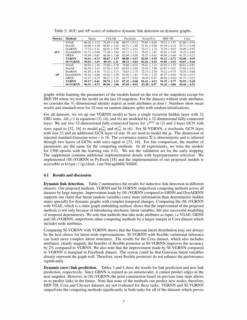
Table 2: AUC and AP scores of inductive dynamic link detection on dynamic graphs.

Metrics Methods Enron COLAB Facebook Social Evo. HEP-TH CoraVGAE 88.26 ± 1.33 70.49 ± 6.46 80.37 ± 0.12 79.85 ± 0.85 79.31 ± 1.97 87.60 ± 0.54DynAE 84.06 ± 3.30 66.83 ± 2.62 60.71 ± 1.05 71.41 ± 0.66 63.94 ± 0.18 53.71 ± 0.48DynRNN 77.74 ± 5.31 68.01 ± 5.50 69.77 ± 2.01 74.13 ± 1.74 72.39 ± 0.63 76.09 ± 0.97

AUC DynAERNN 91.71 ± 0.94 77.38 ± 3.84 81.71 ± 1.51 78.67 ± 1.07 82.01 ± 0.49 74.35 ± 0.85GRNN 91.09 ± 0.67 86.40 ± 1.48 85.60 ± 0.59 78.27 ± 0.47 89.00 ± 0.46 91.35 ± 0.21VGRNN 94.41 ± 0.73 88.67 ± 1.57 88.00 ± 0.57 82.69 ± 0.55 91.12 ± 0.71 92.08 ± 0.35SI-VGRNN 95.03 ± 1.07 89.15± 1.31 88.12 ± 0.83 83.36 ± 0.53 91.05 ± 0.92 94.07 ± 0.44VGAE 89.95 ± 1.45 73.08 ± 5.70 79.80 ± 0.22 79.41 ± 1.12 81.05 ± 1.53 89.61 ± 0.87DynAE 86.30 ± 2.43 67.92 ± 2.43 60.83 ± 0.94 70.18 ± 1.98 63.87 ± 0.21 53.84 ± 0.51DynRNN 81.85 ± 4.44 73.12 ± 3.15 70.63 ± 1.75 72.15 ± 2.30 74.12 ± 0.75 76.54 ± 0.66

AP DynAERNN 93.16 ± 0.88 83.02 ± 2.59 83.36 ± 1.83 77.41 ± 1.47 85.57 ± 0.93 79.34 ± 0.77GRNN 93.47 ± 0.35 88.21 ± 1.35 84.77 ± 0.62 76.93± 0.35 89.50 ± 0.42 91.37 ± 0.27VGRNN 95.17 ± 0.41 89.74 ± 1.31 87.32 ± 0.60 81.41 ± 0.53 91.35 ± 0.77 92.92 ± 0.28SI-VGRNN 96.31 ± 0.72 89.90 ± 1.06 87.69 ± 0.92 83.20± 0.57 91.42 ± 0.86 94.44 ± 0.52

graphs while learning the parameters of the models based on the rest of the snapshots except forHEP-TH where we test the model on the last 10 snapshots. For the datasets without node attributes,we consider the Nt-dimensional identity matrix as node attributes at time t. Numbers show meanresults and standard error for 10 runs on random datasets splits with random initializations.

For all datasets, we set up our VGRNN model to have a single recurrent hidden layer with 32GRU units. All ϕ’s in equations (3), (4), and (6) are modeled by a 32-dimensional fully-connectedlayer. We use two 32-dimensional fully-connected layers for ϕprior in (2) and 2-layer GCN withsizes equal to [32, 16] to model µ(t)

enc and σ(t)enc in (6). For SI-VGRNN, a stochastic GCN layer

with size 32 and an additional GCN layer of size 16 are used to model the µ. The dimension ofinjected standard Gaussian noise ε is 16. The covariance matrix Σ is deterministic and is inferredthrough two layers of GCNs with sizes equal to [32, 16]. For fair comparison, the number ofparameters are the same for the competing methods. In all experiments, we train the modelsfor 1500 epochs with the learning rate 0.01. We use the validation set for the early stopping.The supplement contains additional implementation details with hyperparmaeter selection. Weimplemented (SI-)VGRNN in PyTorch [18] and the implementation of our proposed models isaccessible at https://github.com/VGraphRNN/VGRNN.

4.1 Results and discussion

Dynamic link detection. Table 2 summarizes the results for inductive link detection in differentdatasets. Our proposed methods, VGRNN and SI-VGRNN, outperform competing methods across alldatasets by large margins. Improvement made by (SI-)VGRNN compared to GRNN and DynAERNNsupports our claim that latent random variables carry more information than deterministic hiddenstates specially for dynamic graphs with complex temporal changes. Comparing the (SI-)VGRNNwith VGAE, which is a static graph embedding method, shows that the improvement of the proposedmethods is not only because of introducing stochastic latent variables, but also successful modellingof temporal dependencies. We note that methods that take node attributes as input, i.e VGAE, GRNNand (SI-)VGRNN, outperform other competing methods by a larger margin in Cora dataset whichincludes node attributes.

Comparing SI-VGRNN with VGRNN shows that the Gaussian latent distribution may not alwaysbe the best choice for latent node representations. SI-VGRNN with flexible variational inferencecan learn more complex latent structures. The results for the Cora dataset, which also includesattributes, clearly magnify the benefits of flexible posterior as SI-VGRNN improves the accuracyby 2% compared to VGRNN. We also note that the improvement made by SI-VGRNN comparedto VGRNN is marginal in Facebook dataset. The reason could be that Gaussian latent variablesalready represent the graph well. Therefore, more flexible posteriors do not enhance the performancesignificantly.

Dynamic (new) link prediction. Tables 3 and 4 show the results for link prediction and new linkprediction, respectively. Since GRNN is trained as an autoencoder, it cannot predict edges in thenext snapshot. However, in (SI-)VGRNN, the prior construction based on previous time steps allowsus to predict links in the future. Note that none of the methods can predict new nodes, therefore,HEP-TH, Cora and Citeseer datasets are not evaluated for these tasks. VGRNN and SI-VGRNNoutperform the competing methods significantly in both tasks for all of the datasets which proves

7

Table 3: AUC and AP scores of dynamic link prediction on real-world dynamic graphs.

Metrics Methods Enron COLAB Facebook Social Evo.DynAE 74.22 ± 0.74 63.14 ± 1.30 56.06 ± 0.29 65.50 ± 1.66DynRNN 86.41 ± 1.36 75.7 ± 1.09 73.18 ± 0.60 71.37 ± 0.72

AUC DynAERNN 87.43 ± 1.19 76.06 ± 1.08 76.02 ± 0.88 73.47 ± 0.49VGRNN 93.10 ± 0.57 85.95 ± 0.49 89.47 ± 0.37 77.54 ± 1.04SI-VGRNN 93.93 ± 1.03 85.45 ± 0.91 90.94 ± 0.37 77.84 ± 0.79DynAE 76.00 ± 0.77 64.02 ± 1.08 56.04 ± 0.37 63.66 ± 2.27DynRNN 85.61 ± 1.46 78.95 ± 1.55 75.88 ± 0.42 69.02 ± 1.71

AP DynAERNN 89.37 ± 1.17 81.84 ± 0.89 78.55 ± 0.73 71.79 ± 0.81VGRNN 93.29 ± 0.69 87.77 ± 0.79 89.04 ± 0.33 77.03 ± 0.83SI-VGRNN 94.44 ± 0.85 88.36 ± 0.73 90.19 ± 0.27 77.40 ± 0.43

Table 4: AUC and AP scores of dynamic new link prediction on real-world dynamic graphs.

Metrics Methods Enron COLAB Facebook Social Evo.DynAE 66.10 ± 0.71 58.14 ± 1.16 54.62 ± 0.22 55.25 ± 1.34DynRNN 83.20 ± 1.01 71.71±0.73 73.32 ± 0.60 65.69 ± 3.11

AUC DynAERNN 83.77 ± 1.65 71.99 ± 1.04 76.35 ± 0.50 66.61 ± 2.18VGRNN 88.43 ± 0.75 77.09 ± 0.23 87.20 ± 0.43 75.00 ± 0.97SI-VGRNN 88.60 ± 0.95 77.95 ± 0.41 87.74 ± 0.53 76.45 ± 1.19DynAE 66.50 ± 1.12 58.82 ± 1.06 54.57 ± 0.20 54.05 ± 1.63DynRNN 80.96 ± 1.37 75.34 ± 0.67 75.52 ± 0.50 63.47 ± 2.70

AP DynAERNN 85.16 ± 1.04 77.68 ± 0.66 78.70 ± 0.44 65.03 ± 1.74VGRNN 87.57 ± 0.57 79.63 ± 0.94 86.30 ± 0.29 73.48 ± 1.11SI-VGRNN 87.88 ± 0.84 81.26 ± 0.38 86.72 ± 0.54 73.85 ± 1.33

0 2 4 6 8 10Snapshot

0.075

0.100

0.125

0.150

0.175

0.200

0.225

0.250

Clus

terin

g Co

effic

ient

COLAB Enron Facebook

0 2 4 6 8 10Snapshot

0.004

0.006

0.008

0.010

0.012

0.014

0.016

Dens

ity

COLAB Enron Facebook

Figure 2: Evolution of graph statistics through time.

that our proposed models have better generalization, which is the result of including random latentvariables in our model. We note that our proposed methods improve new link prediction moresubstantially which shows that they can capture temporal trends better than the competing methods.Comparing VGRNN with SI-VGRNN shows that the prediction results are almost the same for alldatasets. The reason is that although the posterior is more flexible in SI-VGRNN, the prior on whichour predictions are based, is still Gaussian, hence the improvement is marginal. A possible avenuefor further improvements is constructing more flexible priors such as semi-implicit priors proposedby Molchanov et al. [17], which we leave for future studies.

To find out when VGRNN and SI-VGRNN show more improvements compared to the baselines,we take a closer look at three of the datasets. Figure 2 shows the temporal evolution of density andclustering coefficients of COLAB, Enron, and Facebook datasets. Enron shows the highest densityand clustering coefficients, indicating that it contains dense clusters who are densely connected witheach other. COLAB have low density and high clustering coefficients across time, which means thatalthough it is very sparse but edges are mostly within the clusters. Facebook, which has both lowdensity and clustering coefficients, is very sparse with almost no clusters. Looking back at (new)link prediction results, we see that the improvement margin of (SI-)VGRNN compared to competingmethods is more substantial for Facebook. Moreover, the improvement margin diminishes whenthe graph has more clusters and is more dense. Predicting the evolution very sparse graphs withno clusters is indeed a very difficult task (arguably more difficult than dense graphs), in which ourproposed (SI-)VGRNN is very successful. The stochastic latent variables in our models can capturethe temporal trend while other methods tend to overfit very few observed links.

8

Figure 3: Evolution of simulated graph topology through time.

Figure 4: Latent representations of the simulated graph in different time steps in 2-d space using VGRNN.

4.2 Interpretable latent representations

To show that VGRNN learns more interpretable latent representations, we simulated a dynamic graphwith three communities in which a node (red colored node) transfers from one community into anotherin two time steps (Figure 3). We embedded the node into 2-d latent space using VGRNN (Figure 4)and DynAERNN (the best performed baseline; Figure S1 in the supplementary material). While theadvantages of modeling uncertainty for latent representations and its relation to node labels (classes)for static graphs have been discussed in Bojchevski and Günnemann [2], we argue that the uncertaintyis also directly related to topological evolution in dynamic graphs.

More specifically, the variance of the latent variables for the node of interest increases in time (left toright) marked with the red contour. In time steps 2 and 3 (where the node is moving in the graph),the information from previous and current time steps contradicts each other; hence we expect therepresentation uncertainty to increase. We also plotted the variance of a node whose communitydoesn’t change in time (marked with the green contour). As we expected, the variance of thisnode does not increase over time. We argue that the uncertainty helps to better encode non-smoothevolution, in particular abrupt changes, in dynamic graphs. Moreover, at time step 2, the moving nodehave multiple edges with nodes in two communities. Considering the inner-product decoder, which isbased on the angle between the latent representations, the moving node can be connected to both ofthe communities which is consistent with the graph topology. We note that DynAERNN (Figure S1)fails to produce such an interpretable latent representation. We can see that VGRNN can separate thecommunities in the latent space more distinctively than what DynAERNN does.

5 Conclusion

We have proposed VGRNN and SI-VGRNN, the first node embedding methods for dynamic graphsthat embed each node to a random vector in the latent space. We argue that adding high level latentvariables to graph recurrent neural networks not only increases its expressiveness to better modelthe complex dynamics of graphs, but also generates interpretable random latent representation fornodes. SI-VGRNN is also developed by combining VGRNN and semi-implicit variational inferencefor flexible variational inference. We have tested our proposed methods on dynamic link predictiontasks and they outperform competing methods substantially, specially for very sparse graphs.

6 Acknowledgments

The presented materials are based upon the research supported by the National Science Foundationunder Grants ENG-1839816, IIS-1848596, CCF-1553281, IIS-1812641 and IIS-1812699. We alsothank Texas A&M High Performance Research Computing and Texas Advanced Computing Centerfor providing computational resources to perform experiments in this work.

9

References[1] Mohammadreza Armandpour, Patrick Ding, Jianhua Huang, and Xia Hu. Robust negative sam-

pling for network embedding. In Proceedings of the AAAI Conference on Artificial Intelligence,volume 33, pages 3191–3198. AAAI, 2019.

[2] Aleksandar Bojchevski and Stephan Günnemann. Deep gaussian embedding of graphs: Unsuper-vised inductive learning via ranking. In International Conference on Learning Representations,2018. URL https://openreview.net/forum?id=r1ZdKJ-0W.

[3] Junyoung Chung, Kyle Kastner, Laurent Dinh, Kratarth Goel, Aaron C Courville, and YoshuaBengio. A recurrent latent variable model for sequential data. In Advances in neural informationprocessing systems, pages 2980–2988, 2015.

[4] Michaël Defferrard, Xavier Bresson, and Pierre Vandergheynst. Convolutional neural networkson graphs with fast localized spectral filtering. In Advances in Neural Information ProcessingSystems, pages 3844–3852, 2016.

[5] Claire Donnat, Marinka Zitnik, David Hallac, and Jure Leskovec. Learning structural nodeembeddings via diffusion wavelets. In International ACM Conference on Knowledge Discoveryand Data Mining (KDD), volume 24, 2018.

[6] Marco Fraccaro, Søren Kaae Sø nderby, Ulrich Paquet, and Ole Winther. Sequentialneural models with stochastic layers. In D. D. Lee, M. Sugiyama, U. V. Luxburg,I. Guyon, and R. Garnett, editors, Advances in Neural Information Processing Systems 29,pages 2199–2207. Curran Associates, Inc., 2016. URL http://papers.nips.cc/paper/6039-sequential-neural-models-with-stochastic-layers.pdf.

[7] Marco Fraccaro, Søren Kaae Sønderby, Ulrich Paquet, and Ole Winther. Sequential neuralmodels with stochastic layers. In Advances in neural information processing systems, pages2199–2207, 2016.

[8] Alias Parth Goyal, Anirudh Goyal, Alessandro Sordoni, Marc-Alexandre Côté, Nan Rose-mary Ke, and Yoshua Bengio. Z-forcing: Training stochastic recurrent networks. InI. Guyon, U. V. Luxburg, S. Bengio, H. Wallach, R. Fergus, S. Vishwanathan, andR. Garnett, editors, Advances in Neural Information Processing Systems 30, pages6713–6723. Curran Associates, Inc., 2017. URL http://papers.nips.cc/paper/7248-z-forcing-training-stochastic-recurrent-networks.pdf.

[9] Anirudh Goyal, Alessandro Sordoni, Marc-Alexandre Côté, Nan Rosemary Ke, and YoshuaBengio. Z-forcing: Training stochastic recurrent networks. In Advances in neural informationprocessing systems, pages 6713–6723, 2017.

[10] Palash Goyal, Nitin Kamra, Xinran He, and Yan Liu. Dyngem: Deep embedding method fordynamic graphs. arXiv preprint arXiv:1805.11273, 2018.

[11] Palash Goyal, Sujit Rokka Chhetri, and Arquimedes Canedo. dyngraph2vec: Capturing networkdynamics using dynamic graph representation learning. Knowledge-Based Systems, 2019.

[12] Aditya Grover and Jure Leskovec. node2vec: Scalable feature learning for networks. InProceedings of the 22nd ACM SIGKDD international conference on Knowledge discovery anddata mining, pages 855–864. ACM, 2016.

[13] Will Hamilton, Zhitao Ying, and Jure Leskovec. Inductive representation learning on largegraphs. In Advances in Neural Information Processing Systems, pages 1024–1034, 2017.

[14] Thomas N Kipf and Max Welling. Variational graph auto-encoders. arXiv preprintarXiv:1611.07308, 2016.

[15] Thomas N Kipf and Max Welling. Semi-supervised classification with graph convolutionalnetworks. In International Conference on Learning Representations, 2017.

[16] Jundong Li, Harsh Dani, Xia Hu, Jiliang Tang, Yi Chang, and Huan Liu. Attributed networkembedding for learning in a dynamic environment. In Proceedings of the 2017 ACM onConference on Information and Knowledge Management, pages 387–396. ACM, 2017.

10

[17] Dmitry Molchanov, Valery Kharitonov, Artem Sobolev, and Dmitry Vetrov. Doubly semi-implicit variational inference. arXiv preprint arXiv:1810.02789, 2018.

[18] Adam Paszke, Sam Gross, Soumith Chintala, Gregory Chanan, Edward Yang, Zachary DeVito,Zeming Lin, Alban Desmaison, Luca Antiga, and Adam Lerer. Automatic differentiation inpytorch. In NIPS-W, 2017.

[19] Bryan Perozzi, Rami Al-Rfou, and Steven Skiena. Deepwalk: Online learning of social repre-sentations. In Proceedings of the 20th ACM SIGKDD international conference on Knowledgediscovery and data mining, pages 701–710. ACM, 2014.

[20] Leonardo FR Ribeiro, Pedro HP Saverese, and Daniel R Figueiredo. struc2vec: Learning noderepresentations from structural identity. In Proceedings of the 23rd ACM SIGKDD InternationalConference on Knowledge Discovery and Data Mining, pages 385–394. ACM, 2017.

[21] Youngjoo Seo, Michaël Defferrard, Pierre Vandergheynst, and Xavier Bresson. Structuredsequence modeling with graph convolutional recurrent networks. In International Conferenceon Neural Information Processing, pages 362–373. Springer, 2018.

[22] Samira Shabanian, Devansh Arpit, Adam Trischler, and Yoshua Bengio. Variational bi-lstms.arXiv preprint arXiv:1711.05717, 2017.

[23] Jian Tang, Meng Qu, Mingzhe Wang, Ming Zhang, Jun Yan, and Qiaozhu Mei. Line: Large-scale information network embedding. In Proceedings of the 24th International Conferenceon World Wide Web, pages 1067–1077. International World Wide Web Conferences SteeringCommittee, 2015.

[24] Rakshit Trivedi, Mehrdad Farajtabar, Prasenjeet Biswal, and Hongyuan Zha. Dyrep: Learningrepresentations over dynamic graphs. In International Conference on Learning Representations,2019.

[25] Mingzhang Yin and Mingyuan Zhou. Semi-implicit variational inference. In InternationalConference on Machine Learning, pages 5660–5669, 2018.

[26] Lekui Zhou, Yang Yang, Xiang Ren, Fei Wu, and Yueting Zhuang. Dynamic network embeddingby modeling triadic closure process. In Thirty-Second AAAI Conference on Artificial Intelligence,2018.

11

Variational Graph Recurrent Neural Networks:Supplementary Material

Ehsan Hajiramezanali†∗, Arman Hasanzadeh†∗, Nick Duffield†, Krishna Narayanan†,Mingyuan Zhou‡, Xiaoning Qian†

† Department of Electrical and Computer Engineering, Texas A&M University{ehsanr, armanihm, duffieldng, krn, xqian}@tamu.edu‡McCombs School of Business, The University of Texas at Austin

mingyuan.zhou@mccombs.utexas.edu

This document contains the detailed discussion of related works, the derivation of the ELBO lowerbound for SI-VGRNN inference, additional dataset details, experimental setups and implementationdetails as well as additional results on interpretability of the derived latent representations.

A Related works

Several dynamic graph embedding methods have been developed using various techniques such asmatrix factorization [23, 21], random walk [20, 7], deep learning [13, 2, 3, 10], and stochastic process[22, 14, 15]. The shortcomings of the existing methods can be categorized as follows:

• Most of these existing methods either capture topological evolution or node attribute changesto learn dynamic node embeddings [18, 11]. But only a few of them model both changessimultaneously [15].

• Some of the existing methods, such as the ones in [22, 2, 21], assume that the temporalpatterns of evolving processes are of short duration and fail to capture long-range temporaldependencies in dynamic networks.

• A common assumption in the literature is that the topological changes are smooth. Themethods with this assumption [2, 21] usually use a regularization term to avoid abruptchanges, which limits their flexibility. Deep learning based models, such as the onesin [10, 3], have been proposed to address this shortcoming; however, these methods onlycare about the topological changes over time but do not model node attribute dynamics orcomplex dependencies between two evolving processes.

• Many of the existing methods, such as [13, 15], cannot model the deletion of nodes or edgeswhich limits their generalizability and flexibility.

• While generative models in form of parametric temporal point processes [14] and deeptemporal point processes [15] have been used for modeling dynamic graphs, none of theexisting methods are capable of modeling the uncertainty of the latent representations.

Our proposed (SI-)VGRNN is the first variational based deep generative model for representationlearning of dynamic graphs. On the contrary to existing methods, (SI-)VGRNN is capable ofinferring the uncertainty of latent representations which is the key in modeling non-smooth changesin dynamic graphs. Moreover, (SI-)VGRNN can capture long-term dependencies in node attributedynamics as well as topological evolution. Furthermore, (SI-)VGRNN can handle node and edgeaddition/deletion.

∗Both authors contributed equally.

33rd Conference on Neural Information Processing Systems (NeurIPS 2019), Vancouver, Canada.

B Lower bound for ELBO in SI-VGRNN

SI-VGRNN posterior can be derived by marginalizing out the mixing distribution as follows,

Z(t) ∼ q(Z(t) |ψt), ψt ∼ qφ(ψt |A(≤t),X(≤t),Z(<t)) = qφ(ψt|A(t),X(t),ht−1),

gφ(Z(t) |A(t),X(t),ht−1) =

∫ψt

q(Z(t) |ψt) qφ(ψt |A(t),X(t),ht−1) dψt .

Based on the first theorem in Yin and Zhou [19], which shows that

KL(Eψ∼qφ(ψ |X,A)[q(Z |ψ)] || p(Z)) ≤ Eψ∼qφ(ψ |X,A)[KL(q(Z |ψ) || p(Z))],

the lower bound for ELBO can be derived as follows,

L =

T∑t=1

L(q(Z(t) |ψt), qφ(ψt |A(t),X(t),ht−1)

)=

T∑t=1

Eψt∼qφ(ψt |A(t),X(t),ht−1)EZ(t)∼q(Z(t) |ψt)log

(p(A(t) |Z(t),ht−1) p(Z(t) |ht−1)

q(Z(t) |ψt)

)

= −T∑t=1

Eψt∼qφ(ψt |A(t),X(t),ht−1)KL

(q(Z(t) |ψt) || p(Z(t) |ht−1)

)+ Eψt∼qφ(ψt |A(t),X(t),ht−1)

EZ(t)∼q(Z(t) |ψt)log p(A(t) |Z(t),ht−1)

≤ −T∑t=1

KL(Eψt∼qφ(ψt |A(t),X(t),ht−1)

q(Z(t) |ψt) || p(Z(t) |ht−1))

+ Eψt∼qφ(ψt |A(t),X(t),ht−1)EZ(t)∼q(Z(t) |ψt)log p(A

(t) |Z(t),ht−1)

=

T∑t=1

EZ(t)∼gφ(Z(t) |A(t),X(t),ht−1)log

(p(A(t) |Z(t),ht−1) p(Z(t) |ht−1)

gφ(Z(t) |A(t),X(t),ht−1)

)= EZ∼q(Z(≤t) |A(≤t),X(≤t))

[log p(A(≤t),X(≤t),Z(≤t))− log q(Z(≤t) |A(≤t),X(≤t))

]= L

While a Monte Carlo estimation of L only requires qφ(Z(t) |ψt) to have an analytic density functionsand qφ(ψt |X(t),ht−1) to be convenient to sample from, the marginal posterior gφ(Z(t) |X(t),ht−1)is often intractable and so the Monte Carlo estimation of the ELBO L is prohibited. SI-VGRNNevaluates the lower bound separately from the distribution sampling. This captures the idea thatcombining an explicit qφ(Z(t) |ψt) with an implicit qφ(ψt |X(t),ht−1) is as powerful as needed, butmakes the computation tractable.

As discussed in [19], if optimizing the variational parameter by climbing L, without stopping theoptimization algorithm early, qφ(ψt |X(t),ht−1) could converge to a point mass density, making SI-VGRNN degenerate to VGRNN. To prevent this problem and inspired by SIVI, we add a regularizationterm to the lower bound as follows,

LK = L+BK ,

where

BK =

T∑t=1

Eψt,ψ

(1)t ,...,ψ

(K)t ∼qφ(ψt |A(t),X(t),ht−1)

KL(q(Z(t) |ψt) || g̃K(Z(t)|A(t),X(t),ht−1)),

g̃K(Z(t) |A(t),X(t),ht−1)) =qφ(ψt |A(t),X(t),ht−1) +

∑Kk=1 qφ(ψ

(k)t |A

(t),X(t),ht−1)

K + 1.

The lower bound leads to an asymptotically exact ELBO that satisfies L0 = L and limK→∞ LK = L.

2

C Additional dataset details

Enron emails (Enron). This graph constructed from 500,000 email messages exchanged between184 Enron employees from 1998 to 2002 [8]. The nodes represent the employees and the edges areemails exchanged between two employees. Following the same procedure as in [17, 9] we clean thedata to get 10 temporal snapshots of the graph. This graph does not have any node or edge attribute.

Collaboration (COLAB). This dataset represents collaborations between 315 authors. Each nodein this dynamic graph is an author and the edges represent co-authorship relationships. The data,provided by Rahman and Al Hasan [9], are collected from years 2000-2009 with a total of 10snapshots considering each year as a time stamp. This COLAB graph does not have any node or edgeattribute.

Facebook. The Facebook wall posts dynamic graph, provided by [16], has 9 time stamps. Followingthe same data cleaning procedure as in [17, 9], we get 663 nodes at each snapshot. No node or edgeattribute is provided for this graph.

HEP-TH. The original dataset [1] covers all the citations of the papers in High Energy PhysicsTheory conference from January 1993 to April 2003 [5]. For each month, we create a citation graphusing all the papers published up to that month. We only consider the first ten months leading to 10snapshots in this dynamic graph. The graph has 1199 nodes at the first month and 2462 at the lastone. This graph also has no node or edge attributes.

Cora. The Cora dataset is another citation graph consists of 2708 scientific publications [12]. Thenodes in the graph represent the publications and the edges indicate the citation relations. Each nodeis provided with a 1433-dimensional binary attribute vector. Each dimension of the attribute vectorindicates the presence of a word in the publication from a dictionary. Originally, Cora is a staticgraph dataset, therefore in order to use it in a dynamic fashion, we preprocess the data as follows inthe same manner as in [6]. We take the indices of nodes as their arriving order in the dynamic graphand add 200 nodes with their corresponding edges, at each temporal snapshot. The dynamic graphincludes 11 snapshots, starting with 708 nodes and reaches to 2708 nodes at the last snapshot.

Social evolution. The social evolution dataset is collected from Jan 2008 to June 30, 2009 andreleased by MIT Human Dynamics Lab [15]. For this dataset, we consider Calls and SMS recordsbetween users as node attributes and all Close Friendship records and Proximity as graph topology.We consider the collected information from Jan 2008 until Sep 10, 2008 (i.e. survey date) to formthe initial network. We used cumulative data for 10 days periods of to form a snapshot of dynamicnetwork for 27 snapshots.

D Details on the experimental setup and hyper-parameters selection

Dynamic autoencoder (DynAE) [3]. This autoencoder model uses multiple fully connected layersfor both encoder and decoder to capture highly non-linear interactions between nodes at each timestep and across multiple time steps. It can take a set of graphs with different adjacency matrices. Thismodel has O(nld1) parameters, where n, l, and d1 are the number of nodes, autoregressive lag, anddimension of the first hidden layer, respectively. Learning to optimize this huge number of parameterscan be challenging for sparse graphs [3], which is often the case when studying real-world datasets.The input to this model at each node is the neighborhood vector of that node.

Dynamic recurrent neural network (DynRNN) [3]. This model uses LSTM networks as bothencoder and decoder to capture the long-term dependencies in dynamic graphs. Comparing toDynAE, the number of parameters is reduced and the model is capable of learning complex temporalpatterns more efficiently. The input to this model at each node is the neighborhood vector of thatnode.

Dynamic autoenncoder recurrent neural network (DynAERNN) [3]. Instead of passing the inputadjacency matrices into LSTM, DynAERNN uses a fully connected encoder to initially acquire lowdimensional hidden representations and then pass them as the input of LSTM to learn the embedding.The decoder of this model is a fully connected network similar to DynAE. The input to this model ateach node is the neighborhood vector of that node.

Experimental setups. For VGAE at each snapshot, we use two GCN layers with 32 and 16 unitsfor GCNµ and GCNσ . Since VGAE is a method for static graph embedding, we start training with

3

Figure S1: Latent representation of the simulated graph in different time steps in 2-d space using DynAERNN.

the first snapshot and use the inferred parameters as initialization for the next snapshot. We continuethis process until the last training snapshot. In all VGAE experiments, the learning rate is set to be0.01. We learn the model for 500 training epochs and use the validation set for the early stopping. Weuse the code provided by the author [4] in our experiments. For DynAE, DynRNN, and DynAERNN,we chose the dimension and number of layers of the encoder and decoder such that the total numbersof parameters is comparable to (SI-)VGRNN. For these methods, we use the source code published bythe authors. In these methods, the learning rate is set to be 0.01 and the learning procedure convergesin 250 training epochs. The look back parameter in these models, which indicates how much in thepast the model looks to learn the embedding, is set to be 2. In all of the experiments in this paper, theembedding dimension is set to 16 except for HEP-TH where embedding dimension is 32.

All of the node embedding methods for link prediction performance comparison are run on a singlecluster node with dual-GPU Tesla K80 accelerator and 128GB RAM. For running each epoch on theHEP-TH dataset using one of the GPUs on this cluster, SI-VGRNN, VGRNN, DynRNN, DynAERNN,and DynAE take around 36, 12, 40, 5, and 1 seconds, respectively. This is expected as DynRNNhas two 2-layer LSTMs as decoders and encoders. On the other hand, the number of parameters inDynAERNN, which includes just one 2-layer LSTM, is less than that of DynRNN. DynAE are fasteras they do not have LSTM units.

E Additional experimental results on interpretability of latent representations

Here, we include the latent representations of the simulated graph (in Section 4.2 of the main text)learned by DynAERNN (shown in Figure S1). Compared to the latent representation learned byVGRNN, not only DynAERNN is not capable of modeling uncertainty of representations, but also itfails to separate the communities of the graph at different time steps, which VGRNN has successfullyaccomplished.

References[1] Johannes Gehrke, Paul Ginsparg, and Jon Kleinberg. Overview of the 2003 kdd cup. ACM

SIGKDD Explorations Newsletter, 5(2):149–151, 2003.

[2] Palash Goyal, Nitin Kamra, Xinran He, and Yan Liu. Dyngem: Deep embedding method fordynamic graphs. arXiv preprint arXiv:1805.11273, 2018.

[3] Palash Goyal, Sujit Rokka Chhetri, and Arquimedes Canedo. dyngraph2vec: Capturing networkdynamics using dynamic graph representation learning. Knowledge-Based Systems, 2019.

[4] Thomas N Kipf and Max Welling. Variational graph auto-encoders. arXiv preprintarXiv:1611.07308, 2016.

[5] Jure Leskovec and Andrej Krevl. SNAP Datasets: Stanford large network dataset collection.http://snap.stanford.edu/data, June 2014.

[6] Xi Liu, Ping-Chun Hsieh, Nick Duffield, Rui Chen, Muhe Xie, and Xidao Wen. Streamingnetwork embedding through local actions. CoRR, abs/1811.05932, 2018.

[7] Giang Hoang Nguyen, John Boaz Lee, Ryan A Rossi, Nesreen K Ahmed, Eunyee Koh, andSungchul Kim. Continuous-time dynamic network embeddings. In Companion Proceedings

4

of the The Web Conference 2018, pages 969–976. International World Wide Web ConferencesSteering Committee, 2018.

[8] Carey E Priebe, John M Conroy, David J Marchette, and Youngser Park. Scan statistics onenron graphs. Computational & Mathematical Organization Theory, 11(3):229–247, 2005.

[9] Mahmudur Rahman and Mohammad Al Hasan. Link prediction in dynamic networks usinggraphlet. In Joint European Conference on Machine Learning and Knowledge Discovery inDatabases, pages 394–409. Springer, 2016.

[10] Aravind Sankar, Yanhong Wu, Liang Gou, Wei Zhang, and Hao Yang. Dynamic graph represen-tation learning via self-attention networks, 2019. URL https://openreview.net/forum?id=HylsgnCcFQ.

[11] Purnamrita Sarkar, Sajid M Siddiqi, and Geogrey J Gordon. A latent space approach to dynamicembedding of co-occurrence data. In Artificial Intelligence and Statistics, pages 420–427, 2007.

[12] Prithviraj Sen, Galileo Namata, Mustafa Bilgic, Lise Getoor, Brian Galligher, and Tina Eliassi-Rad. Collective classification in network data. AI magazine, 29(3):93, 2008.

[13] Youngjoo Seo, Michaël Defferrard, Pierre Vandergheynst, and Xavier Bresson. Structuredsequence modeling with graph convolutional recurrent networks. In International Conferenceon Neural Information Processing, pages 362–373. Springer, 2018.

[14] Rakshit Trivedi, Hanjun Dai, Yichen Wang, and Le Song. Know-evolve: Deep temporalreasoning for dynamic knowledge graphs. In International Conference on Machine Learning,pages 3462–3471, 2017.

[15] Rakshit Trivedi, Mehrdad Farajtabar, Prasenjeet Biswal, and Hongyuan Zha. Dyrep: Learningrepresentations over dynamic graphs. In International Conference on Learning Representations,2019.

[16] Bimal Viswanath, Alan Mislove, Meeyoung Cha, and Krishna P Gummadi. On the evolutionof user interaction in facebook. In Proceedings of the 2nd ACM workshop on Online socialnetworks, pages 37–42. ACM, 2009.

[17] Kevin S Xu and Alfred O Hero. Dynamic stochastic blockmodels for time-evolving socialnetworks. IEEE Journal of Selected Topics in Signal Processing, 8(4):552–562, 2014.

[18] Zhilin Yang, William W Cohen, and Ruslan Salakhutdinov. Revisiting semi-supervised learningwith graph embeddings. arXiv preprint arXiv:1603.08861, 2016.

[19] Mingzhang Yin and Mingyuan Zhou. Semi-implicit variational inference. In InternationalConference on Machine Learning, pages 5660–5669, 2018.

[20] Wenchao Yu, Wei Cheng, Charu C Aggarwal, Kai Zhang, Haifeng Chen, and Wei Wang.Netwalk: A flexible deep embedding approach for anomaly detection in dynamic networks. InProceedings of the 24th ACM SIGKDD International Conference on Knowledge Discovery &Data Mining, pages 2672–2681. ACM, 2018.

[21] Ziwei Zhang, Peng Cui, Jian Pei, Xiao Wang, and Wenwu Zhu. Timers: Error-bounded svdrestart on dynamic networks. In Thirty-Second AAAI Conference on Artificial Intelligence,2018.

[22] Lekui Zhou, Yang Yang, Xiang Ren, Fei Wu, and Yueting Zhuang. Dynamic network embeddingby modeling triadic closure process. In Thirty-Second AAAI Conference on Artificial Intelligence,2018.

[23] Linhong Zhu, Dong Guo, Junming Yin, Greg Ver Steeg, and Aram Galstyan. Scalable temporallatent space inference for link prediction in dynamic social networks. IEEE Transactions onKnowledge and Data Engineering, 28(10):2765–2777, 2016.

5