Variational 3D Shape Segmentation for Bounding Volume ...i.cs.hku.hk/GraphicsGroup/publications/pdf/Variational 3D Shape... · EUROGRAPHICS 2007 / D. Cohen-Or and P. Slavík (Guest

EUROGRAPHICS 2007 / D. Cohen-Or and P. Slavík(Guest Editors)

Volume 26 (2007), Number 3

Variational 3D Shape Segmentation

for Bounding Volume Computation

Lin Lu1, Yi-King Choi1, Wenping Wang1 and Myung-Soo Kim2

1Department of Computer Science, The University of Hong Kong, Hong Kong, China2School of Computer Science and Engineering, Seoul National University, Seoul, South Korea

Abstract

We propose a variational approach to computing an optimal segmentation of a 3D shape for computing a union of

tight bounding volumes. Based on an affine invariant measure of e-tightness, the resemblance to ellipsoid, a novel

functional is formulated that governs an optimization process to obtain a partition with multiple components.

Refinement of segmentation is driven by application-specific error measures, so that the final bounding volume

meets pre-specified user requirement. We present examples to demonstrate the effectiveness of our method and

show that it works well for computing ellipsoidal bounding volumes as well as oriented bounding boxes.

Categories and Subject Descriptors (according to ACM CCS): I.3.5 [Computer Graphics]: Computational Geometryand Object Modeling

1. Introduction

Complex objects are often approximated by simple prim-itives so as to facilitate efficient geometric computa-tions. For this purpose, bounding volumes have beenused very successfully for various applications, includ-ing ray tracing, rendering, collision detection and robusttransmission of geometric data [Bou85, BK02, JTT01,KV05] (Figure 1). There are efficient intersection testsor proximity computations for commonly used boundingvolumes, such as spheres [Hub96], axis-aligned bound-ing boxes (AABBs) [HKM95], oriented bounding boxes(OBBs) [BCG∗96, GLM96], discrete-oriented polytopes (k-DOPs) [KHM∗98] and ellipsoids [RB97, WCC∗04].

The efficiency of a bounding volume for a given objectis often defined as its bounding tightness to the object. Tocompute a proper decomposition of an object into compo-nents so that each can be bounded tightly by a bounding vol-ume is a difficult task. Existing works on computing bound-ing volumes mainly use hierarchical subdivision and encloseeach component with a bounding primitive. The conven-tional top-down hierarchical approach, although fast, is lo-cal and greedy, since there has been no consideration of anoptimization formulation and therefore the previous meth-ods do not allow dynamic updates of different componentsin an optimal manner. Consequently there is still much room

for improvement in bounding tightness. A notable exceptionis the variational approach [WZS∗06] to computing spherebounding volumes; but it is difficult to extend the result toother bounding volumes.

TOV(P) = 0.257MOV(P) = 0.456

Figure 1: The dinopet with its bounding volume (33 ellip-

soids) automatically generated by our algorithm.

A variational approach to computing a partition of anobject often involves data clustering based on Lloyd it-

c© The Eurographics Association and Blackwell Publishing 2007. Published by BlackwellPublishing, 9600 Garsington Road, Oxford OX4 2DQ, UK and 350 Main Street, Malden,MA 02148, USA.

L. Lu, Y.-K. Choi, W. Wang & M.-S. Kim / Variational 3D Shape Segmentation for Bounding Volume Computation

eration [Llo82], a popular heuristic for k-means cluster-ing [KMN∗02]. The most commonly used metric in thisframework is the Euclidean metric, which leads to the stan-dard functional defining the Centroidal Voronoi Tessella-tion (CVT) [DFG99]. The Euclidean metric is isotropic andtherefore cannot capture components with elongated shapes.As we will see in detail at the end of Section 4, the direct useof the anisotropic Mahalanobis (or elliptic) metric [GG89]is problematic, due to its lack of variational foundation. Inthis paper, we propose a fix to this problem by formulating anew anisotropic metric based on an affine invariant conceptof e-tightness, the resemblance to ellipsoid. The new met-ric is more suitable to the problem of computing an optimalsegmentation of a 3D object for the purpose of computinga tight bounding volume. (We caution that such a segmen-tation is not a generally “meaningful” segmentation, so thesegmentation result may not be completely suitable for otherpurposes.)

The main contributions of our work can be summarizedas follows:

1. A new variational formulation is proposed based on

the e-tightness, a function we introduce to measure theresemblance of a set to an ellipsoid. This functional isused to determine an optimal partition of a 3D solid byminimizing a weighted average of the e-tightness func-tions of all components. We present theoretical justifica-

tion of the proposed anisotropic metric. Moreover, wepresent effective computation schemes, and experimentalsupport to show the advantage of this new formulation.

2. Integrating the above optimization method with initial-ization based on skeleton information and error-drivenrefinement of partition, we have devised a complete androbust algorithm for computing a tight bounding vol-

ume composed of the union of ellipsoids or oriented

bounding boxes for complex articulated 3D models, asoften used in computer animation.

2. Previous work

Shape approximation/segmentation. Vast amount of re-search work has been conducted on shape approximation ordecomposition, for a wide range of applications, includingobject recognition and geometry processing. Many ‘greedy’approaches based on local search have been proposed, suchas hierarchical subdivision and region growing, which do notaccommodate dynamic incremental updates of a partitionin a global and optimal manner. Data clustering techniques,e.g., fuzzy clustering [KT03], have also been applied directlyfor shape segmentation. The variational approach has beenadapted in [CSAD04], which computes a piecewise planarapproximation of a surface by minimizing a functional char-acterizing geometric errors. Note that these methods are onlyfor surface decomposition or approximation.

Bischoff and Kobbelt used ellipsoids to cover the in-terior volume of an object [BK02]. The decomposition,

originally designed for surface reconstruction in robust ge-ometry transmission, contains a larger number of ellip-soids than necessary for tight bounding. Simari and Singhachieved ellipsoidal representation of mesh surfaces usingthe Lloyd method with a combination of metrics that con-siders Euclidean radial distance, surface normals and cur-vatures [SS05]. They also introduced a volume metric toobtain ellipsoids approximating a 3D shape. Kalaiah andVarshney proposed the use of k-means clustering with theMahalanobis distance for building a hierarchical PrincipleComponent Analysis (PCA) based representation for a pointset [KV05].

Bounding volume computation. Several geometric primi-tives are commonly used as bounding volumes. The axis-aligned bounding box (AABB) [HKM95] for a given ob-ject is easy to construct, but it does not fit tightly for manyobjects and it has to be recomputed if the orientation ofthe object is changed. The oriented bounding box (OBB)[BCG∗96, GLM96] can fit an object more tightly and theclass of OBBs is closed under any Euclidean transformation.A hierarchy of OBBs, called OBB-tree or box-tree, is oftenused to facilitate fast collision query. The splitting of a par-ent OBB into two smaller components is done by bisectingin the eigen-direction associated with the largest eigenvalueof PCA.

A method for building a hierarchy of spheres, calleda sphere tree, is based on mid-axis surface computa-tion [Hub96]. As an extension to this method, the adaptivemedial axis approximation (AMAA) [BO04] improves thebounding efficiency by refining the segmentation iterativelywith a greedy approach. A bounding sphere set approxima-tion for an object is computed using a variational approachthat minimizes the outside volume of the spheres [WZS∗06].

Statistical and data clustering techniques. Besides k-means clustering, the Expectation Maximization (EM) al-gorithm [Har58] is another general data clustering method,which is widely used in image understanding or medical im-age segmentation. Nevertheless, except for the PCA tech-nique, most statistical and data clustering techniques havenot been applied in relation to computing bounding volumes.

3. Variational formulation

In this section we first define the e-tightness of a point setin E

3, and then use it to formulate a functional whose min-imizer defines an optimal volume segmentation of a givenobject to facilitate the computation of a tight bounding vol-ume.

Given a volume S ⊂ E3, its covariance matrix is

C(S) =∫

x∈S(x−µ)(x−µ)T dσ

∫

x∈Sdσ

,

where dσ is the differential volume and µ =∫

x∈S xdσ/∫

x∈S dσ is the center of mass of S. We in-troduce the Legendre ellipsoid of S, denoted by K(S), as

c© The Eurographics Association and Blackwell Publishing 2007.


K(S) = {x ∈ E3 | xT L−1x≤ 1} [Lei98], where L = 5C(S).

The Legendre ellipsoid is a classical concept in mechanicsand is so defined that K(S)=S when S is an ellipsoid.Note that the Legendre ellipsoid K(S), in general, is not abounding ellipsoid of S (Fig. 2a).

Clearly, the volume of K(S) is

vol(K(S)) = 4π3

√

det(L). (1)

Then we define the e-tightness function of S to be

e(S) =vol(K(S))

vol(S). (2)

In other words, the e-tightness of S is the ratio of the vol-ume of its Legendre ellipsoid to the volume of S. Here wesuppose that S is a compact set of finite but nonzero volume.

We will see next that the e-tightness of a point set S char-acterizes its deviation from the shape of an ellipsoid.

Lemma 1 The e-tightness value of any point set S ⊂ E3 is

invariant under affine transformations.

Proof Denote an affine transformation by T : X = MX +B, where M is a nonsingular matrix describing the linearpart of T . Let C(S) be the covariance matrix of S. Thenit is easy to verify that C(T (S)) = MC(S)MT . It fol-lows that vol(K(T (S))) = det(M) · vol(K(S)). But, sincevol(T (S)) = det(M) · vol(S), by Eq. (2), we conclude thate(T (S)) = e(S).

Lemma 2 e(S)≥ 1 for any set S of finite but non-zero vol-ume in E

3. Furthermore, e(S) = 1 if and only if S is anellipsoid, assuming S is a compact set of finite but nonzerovolume.

Proof The lemma follows from the classical inequality

vol(K(S))≥ vol(S),

where the equality holds if and only if S is an ellip-soid [GLYZ02].

Example 1. Consider the rectangular box R : [−a,a]×[−b,b]× [−c,c]. Its volume is vol(R) = 8abc. Its covariancematrix is C(R) = 8abc

3 diag(a2,b2,c2). Thus its Legendre el-lipsoid K(R) is

(x,y,z) diag(

35a2 , 3

5b2 , 35c2

)

(x,y,z)T ≤ 1.

Then vol(K(R)) = 4·53/2π35/2 abc. So the e-tightness ofR is

e(R) =vol(K(R))

vol(R)= 53/2π

2·35/2 ≈ 1.127.

Due to affine invariance, all rectangular boxes have the samee-tightness.

Next we use the e-tightness to define a functional to char-acterize an optimal partition of a volume. Given a volumeS ⊂E

3, a k-partition of S is denoted byP = {Si}ki=1, where

k≥ 1,⋃

Si = S and Si⋂

S j = ∅ for any i, j with i 6= j. Con-

sequently, ∑ki=1 vol(Si) = vol(S). Then we define a func-

tional F(P) as the weighted average of the e-tightness func-tions of all the components of P , given by

F(P) =k

∑i=1

vol(Si)

vol(S)e(Si). (3)

The minimizer of F(P) characterizes a partition of S thatis optimal in terms of ellipsoidal decomposition, as summa-rized by the following lemma.

Lemma 3 For any k-partition P = {Si}ki=1 of S ⊂ E

3, itholds that F(P) ≥ 1. Furthermore, F(P) = 1 holds if andonly if every component Si of P is an ellipsoid.

Proof By Lemma 2, e(Si)≥ 1. Therefore,

F(P) =k

∑i=1

vol(Si)vol(S)

e(Si)≥k

∑i=1

vol(Si)vol(S)

= 1,

and F(P) = 1 if and only if e(Si) = 1 for every i, or, againby Lemma 2, if and only if every Si is an ellipsoid.

An equivalent expression of F(P) is

F(P) = 1vol(S)

k

∑i=1

vol(K(Si)) =20√

5π/3vol(S)

k

∑i=1

√

det(C(Si)).

(4)Hence, F(P) can be interpreted as the sum of the volumesof the Legendre ellipsoids of all the components Si, normal-ized by the total volume vol(S). Obviously, F(P) is alsoinvariant under affine transformations.

Lemma 3 states that if an object is composed of k disjointellipsoids, a k-partition P can be found such that F(P) = 1,i.e., each component of P is an ellipsoid. However, given anarbitrary object S and a fixed k, such a partition in generalis not possible and so we have F(P) > 1 for any partitionP of S (Fig. 2). It is thus reasonable to say that the par-tition attaining the minimum value of F(P) is statisticallythe best decomposition, in the sense that the volume ratioof the Legendre ellipsoids to the corresponding componentsare minimized. Hence, the minimization of F(P) guides usto obtain a segmentation that facilitates the computation ofbounding volumes, as will be explained in Section 5.

4. Minimization of F(P)

Given the complex expression of F(P) and its dependenceon the shape to be segmented, its minimization cannot beexpected to be straightforward. While there could be severalpotential approaches to designing an effective algorithm, wehave focused on an iterative method that is in spirit simi-lar to the Lloyd iteration. There are two ingredients to such amethod: initialization and iterative update. We shall first dis-cuss our strategy for iterative update and then explain howthe initialization can be set up.

For the sake of computational efficiency, we assume a



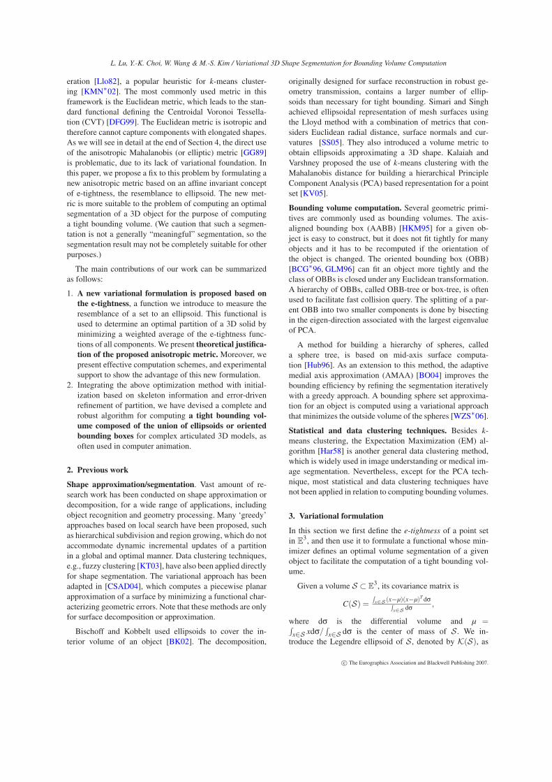
(a) (b) (c)

Figure 2: Three partitions of a bowling pin. The value of

F(P) for (a), (b) and (c) are 1.2097, 1.1116 and 1.0129,

respectively. The components and the bounding ellipsoids

(grey) are shown on the left and the corresponding Legen-

dre ellipsoids (red) on the right.

discrete setting where the volume is given by a set of uni-formly distributed points S = {xi}

ni=1. Clearly, the concepts

introduced in Section 3 can naturally be carried over to thisdiscrete setting. For example, the covariance matrix of S isgiven by

C(S) = 1n

n

∑i=1

(xi−µ)(xi−µ)T ,

where µ = 1n ∑

ni=1 xi is the center of mass of S.

We first use the case of a 2-partition to explain the basicidea. Let the current partition be P = {S1,S2}. Then a keyissue is, according to the basic variational principle, how todetermine the perturbation imposed upon F(P) if one pointin S1 is reassigned to S2, or vice versa. Specifically, takean arbitrary point x ∈ S1, and consider the new partition byP ′ = {S′1,S

′2}, where S′1 = S1 \ {x} and S′2 = S2

⋃

{x}.Clearly, P is a minimizer if F(P) ≤ F(P ′) for any x. Toconvert this into a computational scheme, we must be ableto compute the variation ∆F = F(P ′)−F(P). If ∆F < 0,we accept P ′ as a better partition towards the minimizationof F(P).

In the following we will show that the evaluation of ∆F

leads naturally to an approximate algorithm that is similar tothe k-means clustering but with its Euclidean metric replacedby the Mahalanobis metric weighted by e-tightness.

Proposition 4 The variation in F(P), for reassigning a pointx from S1 to S2 (S1,S2 ∈ P), is given by

∆F = α

[

(

mm−1

)3−

(

mm−1

)3d(x,S1)

m−1 −1

]

det(C(S1))

(

mm−1

) 32

√

(

1− d(x,S1)m−1

)

det(C(S1))+√

det(C(S1))

+

[

(

nn+1

)3+

(

nn+1

)3d(x,S2)

n+1 −1

]

det(C(S2))

(

nn+1

) 32

√

(

1 + d(x,S2)n+1

)

det(C(S2))+√

det(C(S2))

(5)

where m = |S1|, n = |S2|, α =20√

5π/3vol(S)

, and

d(x,Si) = (x−µi)T

C(Si)−1(x−µi), i = 1,2,

are the Mahalanobis distances from x to the centres µ1 andµ2 of S1 and S2, respectively.

Proof The derivation is straightforward but lengthy, so isomitted due to space limitation.

When m = |S1| and n = |S2| are sufficiently large, it isstraightforward to obtain the following approximation:

∆F ≈∆F̃ ≡α

d(x,S2)√

det(

C(S2))

2(n + 1)−

d(x,S1)√

det(

C(S1))

2(m−1)

.

We now consider the case of a k-partition of a volume S.Given a point x ∈ Si, let ∆F̃i, j denote the variation in F dueto the reassignment of x to S j. Then, for sufficiently large|Si| and

∣

∣S j

∣

∣, we have

∆F̃i, j = α

d(x,S j)√

det(

C(S j))

2(|S j|+ 1)−

d(x,Si)√

det(

C(Si))

2(|Si|−1)

≈ γ(

e(S j)d(x,S j)− e(Si)d(x,Si))

, (6)

where d(x,Si) is the Mahalanobis distance from x to thecenter of Si and γ is a positive constant. Here we have usedthe definition of e-tightness by Eqn. (1) and (2), and theapproximation |Si| ≈ vol(Si), since the sampled points inS are sufficiently dense and uniformly distributed. Eqn. (6)implies that, approximately, a weighted Mahalanobis metric(i.e., by the e-tightness) can be used in the k-means frame-work to optimize the functional F(P).

Define h j(x) = e(S j)d(x,S j) for a point x ∈ S. A smallervalue of h j(x) gives a smaller ∆F̃i, j , which favors reassign-ing x to S j . Note that x ∈ Si is reassigned to S` only if ∆F̃i,`

< 0 and ∆F̃i,` < ∆F̃i, j for all j 6= i, `. By Eqn. (6), this isequivalent to assigning x ∈ Si to S` if h`(x) ≤ hi(x) for alli 6= `. For better efficiency and maintaining component con-nectivity, we use a flooding scheme as in [CSAD04] (as-suming 8-neighbor connectivity) to compute a k-partition byminimizing the functional F(P), as shown in the followingalgorithm flow.

ALGORITHM: Minimizing F(P) for a k-partition of a

volume SINPUT: An initial k-partition P = {Si}

ki=1 of S

STEPS:

1. Pcurr←P2. For each point x ∈ S, assign x to S j with h j(x) being the

minimum among all hi(x), i = 1, . . . ,k. Distortion mini-mizing flooding is used in the assignment process.

3. If no point has been reassigned, goto step 6.4. Let Pnew be the new partition formed in step 2. Evaluate

F(Pnew) using Eqn. (4).



(a) (b) (c)

Figure 3: A 2-partition of a 2D shape using different seg-

mentation schemes: (a) k-means clustering with Euclidean

metric; (b) k-means clustering with Mahalanobis metric;

and (c) our scheme of minimizing F(P).

5. If F(Pnew) < F(Pcurr),Pcurr←Pnew, goto step 2.

6. Randomly pick a boundary point y. Let y ∈ Si and let{S j} be the set of components that are adjacent to y.Evaluate ∆Fi, j as in Eqn. (5).If ∆Fi, j < 0 for any S j,

reassign y to S j and goto step 2.If all boundary points of all components cannot be reas-signed,

output F(Pcurr) as the optimized k-partition of S.

Step 6 above serves to check whether the re-grouping per-formed in step 2 is acceptable. This is needed because (a)the criterion ∆F̃ < 0 is only an approximate one; and (b) forefficiency reasons, the covariance matrices C(Si) defininghi(x) are not updated after moving each individual point—they are updated only at the beginning of each iteration, i.e.,after Pnew of the last round is formed. All these affect theaccuracy and therefore, correctness, of this regrouping step.Hence, in step 6, we seek to perturb the boundary points ofthe components in a partition, and see if the reassignment ofany of these boundary points can result in a ∆F < 0, whichin turn will lead to a new partition with smaller F(P).

A Centroidal Voronoi Tessellation (CVT) of k compo-nents of S is used as the initial k-partition for the input ofthe above algorithm. This partition is computed using the k-means clustering based on Euclidean distance with the flood-ing scheme to ensure component connectivity. The initial k-partition can also be obtained by splitting one component ofan optimal (k−1)-partition.

We close this section by giving a geometric interpreta-tion of the Mahalanobis metric in the k-means clustering.Figure 3 shows the 2-partitions of a 2D shape obtained bydifferent schemes, all starting from two reasonably good ini-tial seed points. Since our scheme is closely related to thek-means clustering using the Mahalanobis metric, we expectour method to have similar behavior (Figure 3(c)). Our testsshow that the minimization of F(P) is more robust in global

convergence as it is properly derived from sound variationalprinciples. In contrast, the k-means clustering using the Ma-halanobis metric has the peculiar property [WMSX97] thatthe functional, G(P) = ∑

ki=1 ∑x∈Si

(x− µi)TC(Si)

−1(x−µi), obtained by replacing the Euclidean metric with theMahalanobis metric in the well known functional for theCVT [DFG99], is actually a constant function; that is, it is in-dependent of the number of components in a partition or themanner of partition. This lack of clear variational interpreta-tion is the major obstacle to using the Mahalanobis metric.

5. Complete algorithm

The goal of our complete algorithm for bounding volumecomputation is to segment a 3D shape into multiple com-ponents, so that each component is enclosed tightly by abounding volume. Intuitively, one could think of minimiz-ing the bounding volumes of the components as an objectivefunction to seek an optimal partition; but that would lead to afunctional without explicit expression, making its optimiza-tion intractable. Hence, the algorithm in Section 4 comesinto place by providing a k-partition that minimizes F(P),for a fixed k, as defined in Eqn. (3). The global optimizationis therefore driven so that each component tends to resem-ble the shape of an ellipsoid. However, minimizing F(P)alone is not sufficient for producing a good segmentation forbounding volume computation, due to the following issues.

1. The minimizer of F(P) may be over-optimistic. Considerthe case where a component Si is an ellipsoid with a longbut thin stick attached to it. Since the thin stick is statisti-cally negligible when computing the covariance matrix ofSi, by Lemma 2, e(Si)≈ 1, which suggests a good fitting.However, since the bounding volume is much larger thanits Legendre ellipsoid and contains much empty space, Si

should be further segmented for a tighter bounding.2. The minimizer of F(P) may be over-conservative. Con-

sider a rectangular blockR (with e(R)≈ 1.127; see Ex-ample 1 in Section 3). If it is segmented into two smallerrectangular boxes (which have the same e-tightness1.127, by Lemma 1), then F(P) is still 1.127, indicatingno improvement. However, due to overlapping betweenthe Legendre ellipsoids of the two smaller boxes, the ac-tual bounding tightness has become better if boundingvolumes are computed based on this 2-partition.

Hence, our complete algorithm consists of an iteration oftwo stages. Firstly, we obtain an optimal k-partition P thatminimizes F(P). Next, we validate P by considering someerrors measuring the empty space inside a bounding volume,and refine the segmentation by increasing k, if necessary.

Let BV(Si) denote the bounding volume of Si computedby our algorithm. The global error, TOV(P), measures thenormalized total outside volume, i.e., the space outside S but



inside the union of all bounding primitives, and is defined as

TOV(P) =vol

(⋃

iBV(Si)\S)

vol(S).

The local outside volume of a component Si, denoted byOV(P,Si), measures the normalized volume of the spaceoutside S but inside the bounding volume of Si, and is de-fined as

OV(P,Si) =vol

(

BV(Si)\S)

vol(Si).

We then define the maximum local outside volumeMOV(P) = maxi{OV(P,Si)}, i.e., the maximum local er-ror over all the components of a partition. This volume isevaluated by counting the number of sample points in theregions in question.

We iteratively refine a partition of S by increasing thenumber of components by one at each step, until TOV(P)and MOV(P) are smaller than two pre-defined tolerancesσG and σL, respectively (Figure 4). The flow of the completealgorithm is as follows.

ALGORITHM: Computing the bounding volumes of a

3D shape

INPUT: A 3D shape S and two tolerances σG and σL forthe global and the local error measures, respectively.

STEPS:

1. Sample S by a set of uniformly distributed points.2. Pick a random seed point and form a 1-partition of S.

k← 1.3. Obtain an optimized k-partition, Pk, of S using the algo-

rithm in Section 4 by minimizing F(Pk).4. Compute the bounding volumes BV(Si). Evaluate

TOV(Pk) and MOV(Pk).5. If TOV(Pk) < σG and MOV(Pk) < σL,

goto step 7.6. If TOV(Pk) < TOV(Pk−1),

split S j having the maximum OV(Pk,S j)k← k +1 and go to step 3.

Elsebacktrack to Pk−1 and find the component Sb

with the next largest local outside volume.If no Sb can be found, i.e., all components inPk−1 have been subject to split but failed,

split S j having the maximum OV(Pk,S j)k← k +1 and go to step 3.

Elsesplit Sb and go to step 3.

7. Perform components merge.8. Output the set of bounding volumes BV(Si).

5.1. Splitting components for partition refinement

Step 6 of the above algorithm is a refinement step: we iden-tify the component S j ∈ P

k with the maximum local errorand split it into two, and target at reducing both the total out-side volume and the maximum local outside volume. A splitis done by adding a new seed point which is farthest fromthe centre of S j; then the points in S j are regrouped intotwo components using our optimization scheme in Section4. Such a split will lead to a minimization of a new partitionPk+1. However, in rare cases the optimized partition after asplit may have a larger total outside volume than the previ-ous one. In this case, we backtrack to the old partition Pk

and select the component with the second largest local out-side volume for the next splitting. If all components havebeen attempted but yet the total outside volume cannot bereduced, then we will proceed to split the component withthe largest local outside volume which would lead to an in-crease in the total outside volume. This situation happensrarely because in most cases a split will result in two tighterbounding volumes than the old one. Our tests show that evena backtrack occurs very infrequently.

5.2. Merging components

In a post-processing step of our algorithm, to prevent over-segmentation, we seek to reduce the final number of compo-nents without incurring an increase in the total outside vol-ume. We determine the pair of adjacent components whosemerging will lead to the largest decrease in the total outsidevolume. Merging is then performed for such a pair, and con-tinues iteratively until no possible merge can be identified.

5.3. Computing bounding volumes

Once a 3D volume has been segmented into multiple com-ponents, the next step is to compute the bounding volumefor each component. An approximate minimum-volume en-closing ellipsoid of a component can be computed usingCGAL [FGH∗06] and used as a bounding ellipsoid; how-ever, the method is computationally expensive (almost 6 sec-onds for 10k points). Hence, for efficiency reasons, duringthe intermediate steps of computing the bounding volumesfor evaluating the error measures, we simply apply uniformscalings to the Legendre ellipsoids to bound their corre-sponding components. Only the final bounding ellipsoids foroutput will be computed by CGAL. We also consider the useof OBB [GLM96] as a bounding volume, since the Legen-dre ellipsoid provides the same information as by a PCA.Figure 5 shows that either OBBs or ellipsoids can be a bet-ter choice of bounding volumes, depending on the type ofthe model under consideration. While synthetic objects arebetter bounded by OBBs, our experiments show that objectsof organic forms, such as human characters, are bounded byellipsoids more efficiently.

Our segmentation scheme can be used to set up a bound-



TOV(P) = 2.155MOV(P) = 2.155

k = 1

→

TOV(P) = 1.158MOV(P) = 1.136

k = 2

→ ·· · →

TOV(P) = 0.299MOV(P) = 0.498

k = 13

→

TOV(P) = 0.263MOV(P) = 0.340

k = 11

→

TOV(P) = 0.239MOV(P) = 0.340

k = 10

Splitting components Merging components

Figure 4: The process of segmenting and computing the bounding volume of a teddy bear model, starting from one component

that ends at a 10-partition. The tolerances used are σG = 0.3, σL = 0.5.

(a) 15 OBBs, TOV(P) = 0.336 (b) 15 ellipsoids, TOV(P) = 0.575

(c) 12 OBBs, TOV(P) = 0.627 (d) 12 ellipsoids, TOV(P) = 0.396

Figure 5: OBBs and ellipsoids achieve different degrees of

tightness for different types of objects. The chair ((a) & (b))

is bounded more tightly by OBBs while the hand ((c) & (d))

is bounded more tightly by ellipsoids.

ing volume hierarchy. We first obtain a k-partition (andhence k bounding primitives) to attain a sufficiently tightbounding. We then build the hierarchy bottom up; the com-ponents of two adjacent bounding volumes are grouped andare enclosed tightly by a parent bounding volume. A greedyapproach is used where the grouping is first performed on thepair of ellipsoids that results in the smallest parent boundingvolume. If needed, the k-partition, which comprises the leavenodes of the tree, can be further split in a top-down mannerto obtain lower levels of bounding. Here, splitting of parentbounding volume is determined by a 2-partition optimizationof its component.

5.4. Other error measures

The above volume-based error measures used to govern seg-mentation refinement can also be replaced by other kindsof error measurement, depending on specific applications.While the volume-based errors are relevant to collisiondetection, restricting the Hausdorff distance between thebounding volume B and the object boundary O can be use-ful for shadow computation, for example, since it provides amore perception-sensitive measure. Different error measurescan be used in combination. In this case, the segmentation re-finement terminates when the thresholds for all the metricsare satisfied.

6. Implementation issues

6.1. Segmentation for skeleton-based volumes

Extracting the skeleton of an object, especially an articulatedobject as commonly used in animation, has been well stud-ied. Any approximate skeletal structure is good enough asan initial input to our algorithm. We assign a seed point toeach link that naturally defines a component in the partition.A CVT is used as an initial partition for the optimization asdescribed in Section 4 for obtaining a k-partition with fixedk. This saves much computation time that would otherwisebe spent on building the k-partition from a single initial com-ponent (Figure 6).

6.2. Efficiency vs. quality

The computational efficiency depends highly on the numberof samples taken from the 3D volume. While an overly highsampling rate leads to slow computation, a sparse samplingcould easily induce errors to the bounding volumes, sincefine parts of an input object, often important as features,may receive too few sample points. We use two techniques,multi-grid and adaptive sampling, in a preprocessing step tobalance segmentation quality and computational time.

Multi-grid. We apply a discrete multi-grid technique wherea progressively finer sampling is used as the Lloyd iterations



Figure 6: Segmentation of a 3D shape with skeleton. (Left)

Initial fitting with 22 bounding ellipsoids (TOV(P) = 0.434,

MOV(P) = 1.175); (right) Segmentation output with 30

bounding ellipsoids using σG = 0.3 and σL = 0.4 (TOV(P) =

0.298, MOV(P) = 0.336).

Figure 7: More points are sampled in regions of small fea-

tures, e.g., the fingers, so that they can be bounded tightly.

proceed. A pre-computed multiresolution point sampling ofthe volume is maintained. The results of an optimized parti-tioning of a coarse level is transferred to the next finer levelby copying the assignments of sample points to their cor-responding points at the finer grid, thus providing a goodinitialization to facilitate faster convergence.

Adaptive sampling. Each sample point is associated withits distance to the shape boundary by applying a medial-axis transform [ACK01] at a preprocessing step. Wheneveran optimized partition is computed, we evaluate the aver-age distance to the shape boundary over all points in eachcomponent. An average distance smaller than a predefinedthreshold indicates a possible feature and therefore a densersampling is used. Each sample point then carries a weightproportional to the volume it represents, so that a point in amore densely sampled region contributes less in the Legen-dre ellipsoids computations and error evaluations. Figure 7shows a segmentation of a human character with each fingerproperly and tightly bounded by an ellipsoid using adaptivesampling.

7. Experimental results and discussions

Figure 8 shows the 20-partitions of a human model (15Ksample points) obtained by a CVT (1.8 seconds) and our

TOV(P) = 0.501, MOV(P) = 2.348 TOV(P) = 0.369, MOV(P) = 1.222

Figure 8: Segmentation of a human character obtained by

(left) the CVT method; and (right) our algorithm. Both con-

tain 20 components, and our method can automatically de-

compose the limbs properly.

method (4 seconds with optimization on the partition only,without any splitting or merging of components). The CVTmethod generates components corresponding to the Voronoicells and hence cannot capture some elongated shapes espe-cially at the limbs. Our algorithm, on the other hand, showssuperiority over the commonly used CVT method, due tothe anisotropic nature in the metrics that we use. There is asignificant difference between the anisotropy of our methodand that of some other anisotropic data clustering methodswhich use a fixed Riemannian metric; the anisotropy used inthis paper varies as the partition is improved progressively.

Figure 9 shows the results of applying our algorithm tosome complex models. The running time of our algorithmdepends on several factors, such as the number of samplepoints, the type of bounding volumes, and the user-specifiedtolerances that control the degree of segmentation refine-ment. With 20K sample points, our algorithm takes 2 min-utes to generate the 33 bounding ellipsoids for the dinopetas shown in Figure 1. The use of skeletal information resultsin significant speedup—the bounding ellipsoids for the horse(20K points) (Figure 6) are computed in 30 seconds only. Alltiming results are taken on a 1.66GHz Pentium IV computerwith 1GB RAM.

8. Conclusion

We presented a novel algorithm in computing a segmenta-tion for bounding volume computation based on a new func-tional, for which we provided theoretical justifications. Ourexperimental results show that the proposed algorithm canproduce a shape decomposition that is more shape adaptive,as compared to segmentation using k-means clustering withthe Euclidean metric. Combined with other error measure,such as the total outside volume, our algorithm is capable ofproducing tight bounding volumes.

We point out that the formulation of the functional F(P)in Eq.(3) is not the only way of utilizing the concept of e-tightness. Other formulations and their behaviors remain to



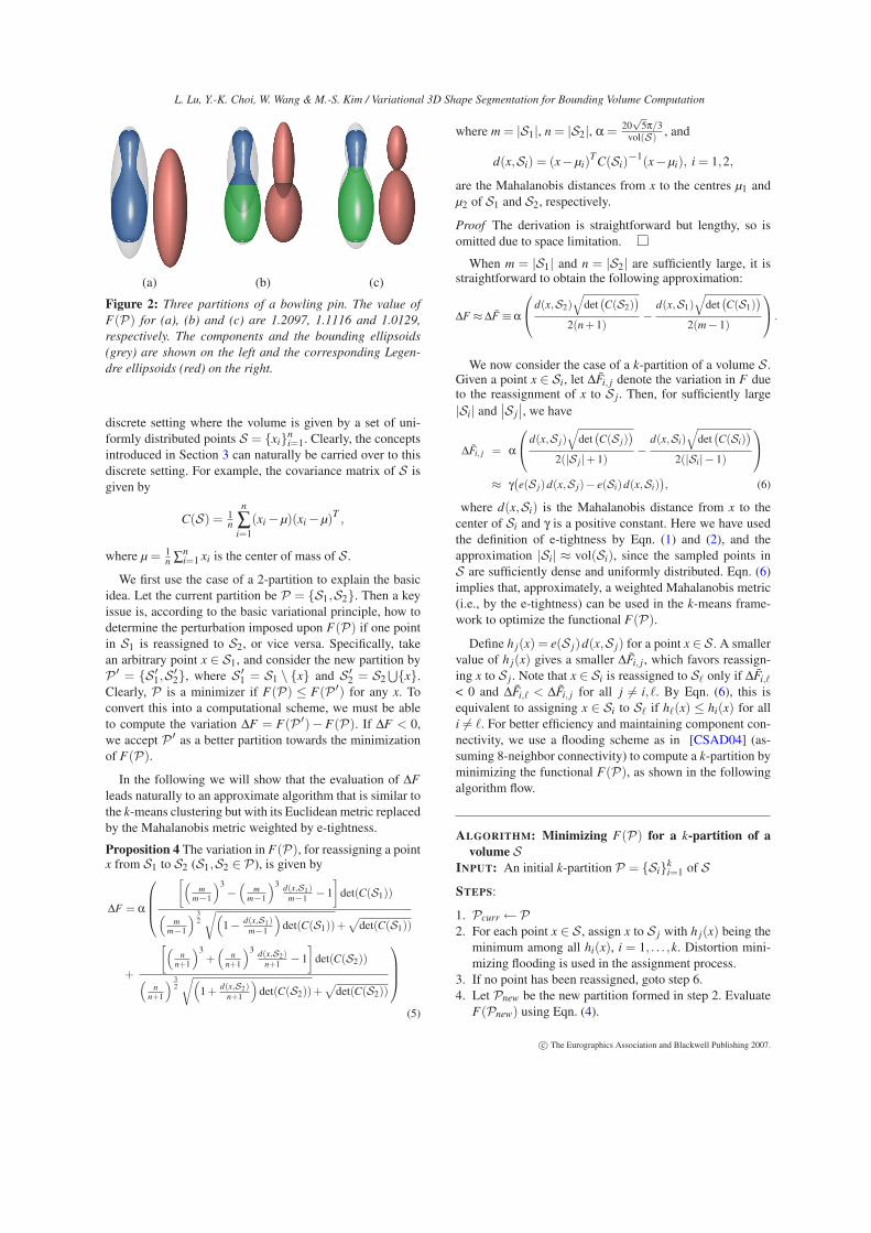
TOV(P) = 0.262, MOV(P) = 0.436(a) 31 ellipsoids

TOV(P) = 0.350, MOV(P) = 0.440(b) 33 ellipsoids

TOV(P) = 0.261, MOV(P) = 0.428(c) 27 ellipsoids

TOV(P) = 0.292, MOV(P) = 0.497(d) 38 ellipsoids

TOV(P) = 0.486, MOV(P) = 0.897(e) 18 OBBs

TOV(P) = 0.380, MOV(P) = 1.302(f) 16 OBBs

Figure 9: Results of our algorithm on different models.

be studied. We also wish to study the effect of using addi-tional local geometric features, such as surface curvature, fora better control in the resulting partition. Finally, the feasi-bility of adopting our algorithm for computing the boundingvolume of dynamic or deformable objects will be exploredin future work.

Acknowledgements

We would like to thank anonymous reviewers for their in-valuable comments. The work of Wenping Wang was par-tially supported by the National Key Basic Research Projectof China (2004CB318000), the Research Grant Council ofHong Kong (HKU 7178/06E), and the Innovative and Tech-nology Fund of Hong Kong (ITS/090/06). This research wasalso supported in part by the Korean Ministry of Informationand Communication (MIC) through the IT Research Centerfor CCGVR.

References

[ACK01] AMENTA N., CHOI S., KOLLURI R. K.: Thepower crust, unions of balls, and the medial axis trans-form. Comput. Geom. 19, 2-3 (2001), 127–153.

[BCG∗96] BAREQUET G., CHAZELLE B., GUIBAS L. J.,MITCHELL J. S. B., TAL A.: BOXTREE: A hierarchicalrepresentation for surfaces in 3D. Comput. Graph. Forum

15, 3 (1996), 387–396.

[BK02] BISCHOFF S., KOBBELT L.: Ellipsoid decompo-

sition of 3D-model. In IEEE 3DPVT (2002), pp. 480–489.

[BO04] BRADSHAW G., O’SULLIVAN C.: Adaptivemedial-axis approximation for sphere-tree construction.ACM Trans. Graph. 23, 1 (2004), 1–26.

[Bou85] BOUVILLE C.: Bounding ellipsoids for ray-fractal intersection. In SIGGRAPH ’85, pp. 45–52.

[CSAD04] COHEN-STEINER D., ALLIEZ P., DESBRUN

M.: Variational shape approximation. In SIGGRAPH ’04,pp. 905–914.

[DFG99] DU Q., FABER V., GUNZBURGER M.: Cen-troidal Voronoi tessellations: Applications and algo-rithms. SIAM Rev. 41, 4 (1999), 637–676.

[FGH∗06] FISCHER K., GARTNER B., HERRMANN T.,HOFFMANN M., PACKER E., SCHONHERR S.: Geomet-ric optimisation. In CGAL-3.2 User and Reference Man-

ual, Board C. E., (Ed.). 2006.

[GG89] GATH I., GEVA A. B.: Unsupervised optimalfuzzy clustering. IEEE Trans. Pattern Anal. Mach. Intell.

11, 7 (1989), 773–780.

[GLM96] GOTTSCHALK S., LIN M. C., MANOCHA D.:OBBTree: A hierarchical structure for rapid interferencedetection. In SIGGRAPH ’96, pp. 171–180.

[GLYZ02] GULERYUZ O. G., LUTWAK E., YANG D.,ZHANG G.: Information-theoretic inequalities for con-toured probability distributions. IEEE Trans. on Informa-

tion Theory 48, 8 (Aug. 2002), 2377–2383.



[Har58] HARTLEY H.: Maximum likelihood estimationfrom incomplete data. Biometrics 14 (1958), 174–194.

[HKM95] HELD M., KLOSOWSKI J. T., MITCHELL J.S. B.: Evaluation of collision detection methods for vir-tual reality fly-throughs. In Seventh Canadian Conference

on Computational Geometry (1995), pp. 205–210.

[Hub96] HUBBARD P. M.: Approximating polyhedra withspheres for time-critical collision detection. ACM Trans.

Graph. 15, 3 (1996), 179–210.

[JTT01] JIMÉNEZ P., THOMAS F., TORRAS C.: 3D col-lision detection: a survey. Computers & Graphics 25, 2(2001), 269–285.

[KHM∗98] KLOSOWSKI J. T., HELD M., MITCHELL J.S. B., SOWIZRAL H., ZIKAN K.: Efficient collision de-tection using bounding volume hierarchies of k-DOPs.IEEE Trans. Vis. Comput. Graph. 4, 1 (1998), 21–36.

[KMN∗02] KANUNGO T., MOUNT D. M., NETANYAHU

N. S., PIATKO C. D., SILVERMAN R., WU A. Y.: Anefficient k-means clustering algorithm: Analysis and im-plementation. IEEE Trans. Pattern Anal. Mach. Intell. 24,7 (2002), 881–892.

[KT03] KATZ S., TAL A.: Hierarchical mesh decomposi-tion using fuzzy clustering and cuts. ACM Trans. Graph.

22, 3 (2003), 954–961.

[KV05] KALAIAH A., VARSHNEY A.: Statistical geome-try representation for efficient transmission and rendering.ACM Trans. Graph. 24, 2 (2005), 348–373.

[Lei98] LEICHTWEISS K.: Affine Geometry of Convex

Bodies. Johann Ambrosius Barth, Heidelberg, 1998.

[Llo82] LLOYD S. P.: Least squares quantization in PCM.IEEE Transactions on Information Theory 28, 2 (1982),129–136.

[RB97] RIMON E., BOYD S. P.: Obstacle collision detec-tion using best ellipsoid fit. J. Intell. Robotics Syst. 18, 2(1997), 105–126.

[SS05] SIMARI P. D., SINGH K.: Extraction and remesh-ing of ellipsoidal representations from mesh data. In Pro-

ceedings of Graphics Interface ’05, pp. 161–168.

[WCC∗04] WANG W., CHOI Y.-K., CHAN B., KIM M.-S., WANG J.: Efficient collision detection for movingellipsoids using separating planes. Computing 72, 1-2(2004), 235–246.

[WMSX97] WANG S., MA F., SHI W., XIA S.: The hy-perellipsoidal clustering using genetic algorithm. In IEEE

ICIPS ’97 (1997), pp. 592–596.

[WZS∗06] WANG R., ZHOU K., SNYDER J., LIU X.,BAO H., PENG Q., GUO B.: Variational sphere set ap-proximation for solid objects. The Visual Computer 22,9-11 (2006), 612–621.


Documents

Variational 3D Shape Segmentation for Bounding Volume ...i.cs.hku.hk/GraphicsGroup/publications/pdf/Variational 3D Shape... · EUROGRAPHICS 2007 / D. Cohen-Or and P. Slavík (Guest