Variation of Surface Air Temperature in Complex Terrain

Variation of Surface Air Temperature in Complex Terrain

L. MAHRT

College of Oceanic and Atmospheric Sciences, Oregon State University, Corvallis, Oregon

(Manuscript received 11 October 2005, in final form 18 February 2006)

ABSTRACT

Data from three micronetworks with eddy correlation data and three additional micronetworks withouteddy correlation data are analyzed to study the spatial variability of surface air temperature in complexterrain. A simple similarity relationship is constructed to relate the spatial variation of air temperature alongthe slope to the thermal forcing and mixing. Mixing is not included in present empirical formulations of thesurface air temperature distribution in complex terrain. The development of surface temperature gradientsalong the slope, resulting from surface heating or cooling, is bounded by a maximum (or saturated) value,where a further increase of temperature gradients is restricted by redistribution of heat by thermally drivenslope circulations. Although much of the spatial variation of the surface air temperature is governed bycomplex three-dimensionality and surface vegetation, a relatively simple relationship is able to account formuch of the diurnal and day-to-day variation of the spatial distribution of air temperature. This relationshiprequires information on the surface heat flux and friction velocity over a reference surface. Requiredgeneralizations of the relationship are outlined before it can be applied to an arbitrary site.

1. Introduction

The spatial distribution of surface air temperature incomplex terrain depends on the three-dimensional to-pography, vegetation, soil characteristics, net radiation,and speed of the large-scale flow. Predicting the varia-tion of surface air temperature with surface elevation(terrestrial temperature gradient) is very complex, al-though a number of simplifications are possible forsome circumstances.

Acevedo and Fitzjarrald (2001, their Fig. 3) find thata height-independent terrestrial temperature gradientis a reasonable approximation at night, subject to de-viations associated with sheltering by small-scale con-cave curvature of the terrain corresponding to trappingof cold air in low-lying areas. Even weak curvature ofthe terrain can influence the local heat budget (Haidenand Whiteman 2005). Height-independent terrestrialtemperature gradients have been assumed by Hocevarand Martsolf (1971), Pielke and Mehring (1977), Listonet al. (1999) and numerous other investigations.LeMone et al. (2003) find that over gentle terrain in

south central Kansas, the nocturnal air temperature at2 m is generally a linear function of surface elevation,corresponding to the height-independent terrestrialtemperature gradient. Deviations from the linear de-pendence of air temperature on surface elevation wererelated to variations of vegetation and pooling of coldair in low-lying areas.

Valleys with steeper slopes are more protected fromthe overlying ambient flow and are less coupled to thefree-atmospheric vertical temperature gradient. Ace-vedo and Fitzjarrald (2001) relate the nocturnal airtemperature to the deviation of the surface height froma small-scale average. The effect of terrain curvaturemay correspond to flow of cold-air drainage over thetop of the trapped colder air at the bottom of the slope(e.g., Heywood 1933; Yoshino 1975; Mahrt et al. 2001).Mahrt and Heald (1983) found that the nocturnal sur-face radiation temperature was more closely related toterrain curvature than surface elevation over undulat-ing terrain. They also found that the role of slope anglewas significant; apparently warmer air temperaturesover steeper slopes result from stronger drainage flowsand greater downward mixing of heat toward the sur-face. With significant ambient flow, they also found adownwind phase shift of the surface temperature withrespect to the undulating terrain.

Slopes with larger vertical extent may be character-

Corresponding author address: Larry Mahrt, College of Oceanicand Atmospheric Sciences, Oregon State University, Corvallis,OR 97331-5503.E-mail: [email protected]

NOVEMBER 2006 M A H R T 1481

© 2006 American Meteorological Society

JAM2419

ized by a thermal belt where the surface air tempera-ture reaches a maximum, often a few hundred metersabove the valley floor (Yoshino 1975). Above the ther-mal belt, the surface air temperature decreases withsurface height and may be influenced by the verticaltemperature gradient of the free atmosphere. Addi-tional discussion is provided by Whiteman (2000, seehis schematic Fig. 11.4.). The thermal belt is sometimesfound over the steepest part of the slope (Yoshino1984) and is apparently caused by acceleration of coldair down the slopes, leading to shear-generated mixingof heat downward toward the sloped surface. The mod-erated cold-air drainage then flows out over the “cold-air lake” at the bottom of the slope. Terms, such ascold-air lake and thermal belt, are not precisely de-fined. In fact, Whiteman (2000) points out that noctur-nal surfaces of constant potential temperature in valleysbend upward toward the side slopes in contrast to thewater analogy. Greater cooling of the air at the bottomof valleys with convex side slopes, as compared withthose with concave side slopes, can be produced by thesmaller volume of air in the valleys with convex side-walls, as noted by Whiteman (2000).

Values of the nocturnal terrestrial temperature gra-dient vary dramatically. For three selected nights, Ace-vedo and Fitzjarrald (2001, their Fig. 5) found that theterrestrial potential temperature gradient was about 10K (100 m)�1 over a surface elevation range of 50 m.Richardson et al. (2004) find that along the slopes of thelargest topographical features in the northeasternUnited States, extending 1500 m vertically, the noctur-nal terrestrial potential temperature gradient is onlyabout 0.5 K (100 m)�1. They averaged over all of thenights, including cloudy, windy nights. Clements et al.(2003) found a very large value of 32 K (100 m)�1 in a150-m-deep sinkhole. Yoshino (1984) reported that ter-restrial potential temperature gradients average about8 K (100 m)�1 near the bottom of a slope of 700-mvertical extent with wintertime clear-sky conditions.The values were somewhat smaller in summer. For se-lected days over rolling landscape, examined by LeMoneet al. (2003), the average value of the terrestrial poten-tial temperature gradient was about 8 K (100 m)�1.

The spatial variation of surface air temperature canoccur simultaneously over a continuum of horizontalscales. These scales can be arbitrarily organized intosmaller microscale variations such as hills, valleys, gul-lies and frost pockets, and larger-scale terrain forms(e.g., Kimura and Kuwagata 1993; Kurita et al. 1990).Local circulations are expected to be more dominantclose to the surface and regional circulations moredominant at higher levels, if they exist (Mahrt et al.2001). On the other hand, Whiteman et al. (2000b)

found that the regional circulation associated with con-trasts between the Mexican Plateau/basin and the ma-rine air prevented normal development of local slopecirculations and of strong nocturnal surface inversions.Other examples of dominance by regional circulationswere found by Stewart et al. (2002). Tabony (1985)divided the impact of terrain on nocturnal air tempera-tures into two horizontal scales—one on the order of 3km and less, and one on the order of 10 km. In terms ofnumerical models, the terrain-induced variations arepartitioned into subgrid and grid-resolved variations.

The daytime spatial distribution of surface air tem-perature can be more complex because it is forced bysolar irradiance, which depends directly on the three-dimensionality of the topography with respect to solarzenith and azimuthal angles. The effect of slope mag-nitude on nocturnal net radiative cooling appears to besmall for weak-to-moderate slope but is significant fordaytime conditions (Nie et al. 1992). In addition, spatialvariations of vegetation and soil moisture can lead todramatic variations of the daytime surface energy bud-get and heating of the atmosphere (Whiteman et al.1989).

Moore et al. (1993), Thorton et al. (1997), Daly et al.(2002), and Bellasio et al. (2005) employ a specifiedlapse rate with a correction term for slope aspect, sur-face heating, and vegetation. Using a similar approach,Chung and Yun (2004) inferred that the variation ofevapotranspiration contributes significantly to thevariation of the relationship between air temperatureand solar radiation at their sites. Bellasio et al. (2005)have incorporated the influence of surface elevation,slope aspect, and vegetation on local air temperaturevariations into a diagnostic meteorological model(“CALMET”) and found improved comparisons withobservations.

These models of the daytime spatial distribution ofsurface air temperature use fairly complete treatmentsof the solar radiation intercepted by an arbitrary in-clined surface, but do not explicitly include the limitinginfluence of turbulent mixing and local (unresolved)transport of heat. Part of the redistribution of heat isdue to local slope circulations and part is related to theinfluence of the larger-scale flow on mixing, such asrepresented by the Froude number (LeMone et al.2003). At a given site, the terrestrial temperature gra-dient decreases with wind speed (Gustavsson et al.1998), probably reflecting the influence of increasedturbulent mixing. Bootsma (1976) found that, among alist of possible influences, the spatial variation of noc-turnal surface temperatures was most related to windspeed and the opacity of the atmosphere.

The goal of the current study is to understand and

1482 J O U R N A L O F A P P L I E D M E T E O R O L O G Y A N D C L I M A T O L O G Y VOLUME 45

formulate the day-to-day variations of the terrestrialtemperature gradient, as forced by surface heating/cooling and reduced by mechanical mixing and trans-port of heat by the regional and large-scale flow. Thisstudy will attempt to formulate such influences on thetemperature distribution along the slope for possibleinclusion in a model that also includes the spatial dis-tribution of vegetation and absorption of solar radia-tion.

2. Data

a. Instrumentation

We analyze data from six micronetworks, which in-clude the Hobo Pro datalogger (Onset Computer Cor-poration, model H08-031-08) and thermistor (White-man et al. 2000a; Nakamura and Mahrt 2005) enclosedin naturally ventilated multiplate shields (Davis Instru-ments, model 7714). Temperature measurements aretaken at 0.5 m above the estimated “displacementheight,” taken to be a fraction of the vegetation height.The fraction was specified to decrease with increasingsparseness of the vegetation. However, because theMonin–Obukhov similarity theory is not expected to bevalid above the understory, there is no theoreticallybased method for estimating such displacement heightsand the problem remains unsolved (Nakamura andMahrt 2005). Five-minute averages of temperature arerecorded and then averaged over 1 h for the analyses ofthis study.

Four of the micronetworks include a limited numberof Handar two-dimensional sonic anemometers that arecapable of measuring wind speeds down to a few cen-timeters per second. Three of the micronetworks in-clude a central tower with profiles of wind and tem-perature and eddy correlation measurements at one ormore levels using Campbell Scientific, Inc., CSAT sonicanemometers.

b. Sites

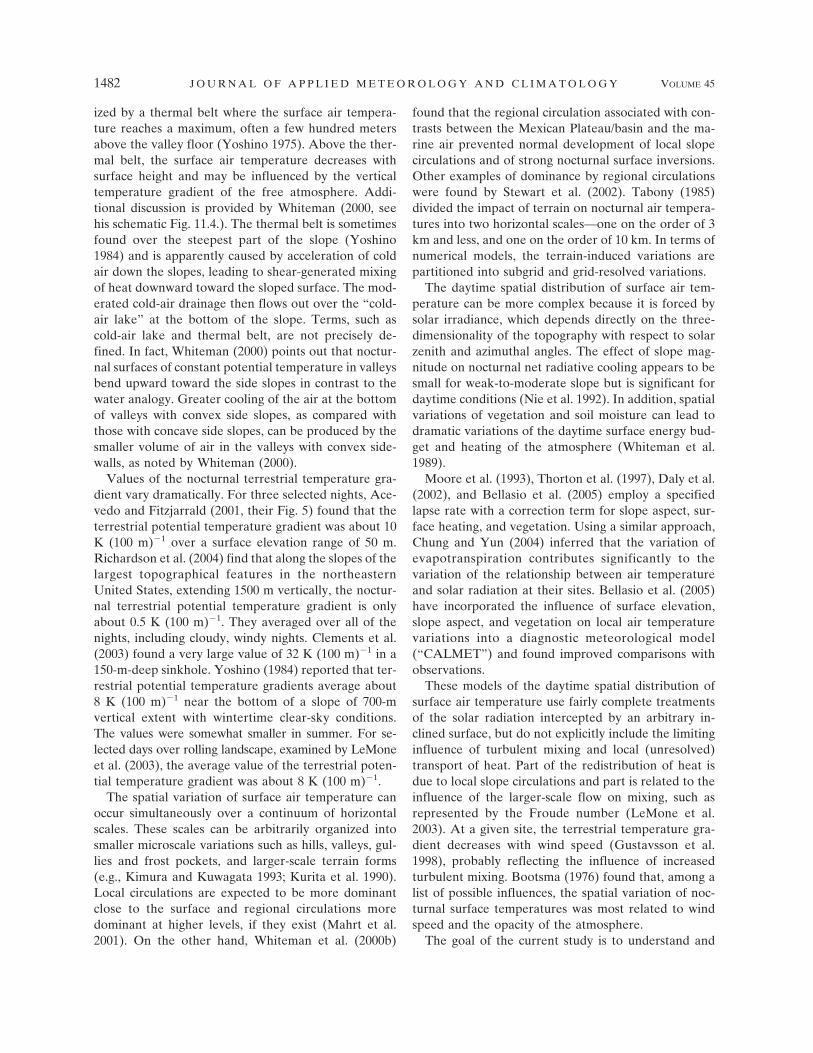
Basic topographical information for the measure-ment sites is included in Table 1. The north-facingEyerly slope in central Oregon has an average slope ofabout 20% (Fig. 1) over a total elevation gain of 200 m,with maximum slope occurring over the upper half ofthe slope. The opposing south-facing slope has an el-evation gain of only about 50 m. The valley and slopesare covered by sparse ponderosa pine, part of which hasbeen recently burned. A 17-m tower in the valley pro-vides eddy correlation measurements at 10 m, windprofiles from Handar sonic anemometers, Hobo tem-perature profiles, and radiation measurements. Thir-

teen additional thermistors were deployed on theground, nine of them are in a cross-valley transect. Thedata period extends from 6 June 2004 until 27 Decem-ber 2004.

The young pine site in central Oregon (Fig. 1) in-cludes a transect of five Hobos extending from a gullybottom eastward up the slope, which gradually de-creases with height. At higher levels, the slope becomessteeper again in association with an isolated roundmountain, which was not instrumented. The height ofthe ponderosa pine averages about 3 m with variabledensity along the transect. Wind and temperature pro-files, radiation, and eddy correlation data were col-lected from a tower on a small ridge, about 200 m to thesouth of the gully (Schwarz et al. 2004). The data periodis from 1 April 2002 until 30 September 2002.

The juniper site in central Oregon (Fig. 1) includes atransect of four thermistors from a hilltop downward to

FIG. 1. Surface elevation profile for the three sites with eddycorrelation data. In all three cases, the main instrumentationtransect is on the left slope and extends to the top of the slope forthe Eyerly and juniper sites and the top of the well-defined slopefor the pine site.

TABLE 1. Eddy correlation datasets. Averaged slope, total el-evation gain, azimuth (0° is north facing), and average down-valley slope.

SiteSlope(%)

Elevgain (m)

Azimuth(°)

Down-valleyslope (%)

Eyerly 20 200 0 4Juniper 8.5 14 135 �1Young pine 9 58 240 4Hampton Gulley 6 11 70 1.2Lower Starker-Bear 50 55 300 1Upper Starker-Bear 27 800 180 1Walnut Hill 20 90 180 0


the bottom of a gully, descending a vertical distance ofonly 14 m. The height of the sparse juniper averagesabout 3 m with a leaf area index (LAI) of about 1. Thetop of the hill had eddy correlation measurements aswell as radiation data. The data period covers from 19July 2002 to 3 November 2003.

We also collected data on three micronetworks withno eddy correlation measurements. The Walnut Hilltransect is on a grass-covered south-facing slope with anaverage slope magnitude of 20% and a 90-m elevationgain. This site can be viewed as a miniature version ofthe plains–slope configuration. Fourteen Hobo ther-mistors were deployed along the slope in 2003. TheStarker-Bear Trail dataset in the coastal range of west-ern Oregon consists of a network within a recentlyplanted clear cut at the bottom of a deep valley, ap-proximately 100 m above sea level. A second transecton one of the higher slopes extends from approximately400 to 1000 m above sea level. For this study, we haveused summer data from 2002 when the network was themost complete. Fluxes over snow-covered surfaces(FLOSS) in North Park Colorado (Mahrt and Vickers2005) included a micronetwork of eight Hobos de-ployed across Hampton gully, located 5 km to thenorth-northeast of the main tower. Eddy correlationdata were collected only in winter. Here we analyzedata only for the summer period.

The large-scale flow was evaluated above the localcirculations at the Eyerly and pine sites, using windsmeasured at the top of a 31-m tower on a nearby el-evated flat area. However, even at this level, the windspeed and direction varied diurnally and were signifi-cantly correlated with the slope flows at the Eyerly site.These higher-level winds seem to be part of a regionalcirculation responding to larger-scale slopes. A re-gional-scale circulation is found east of the CascadesMountains in Washington State (Doran and Horst1983; Doran and Zhong 1994), thought to be a combi-nation of cold-air drainage and a larger-scale regionalpressure gradient that is thermally forced by cooler airwest of the Cascades. Because the diurnal variation ofthese regional winds and the local valley and slopeflows are correlated, they do not provide statisticallyindependent information for study of the terrestrialtemperature gradient.

c. Analysis

The Hobo data were not corrected for radiativelyinduced temperature errors (Nakamura and Mahrt2005) because we were unable to estimate the solarradiation for each individual thermistor in the sub-canopy. For open micronetworks with no overstory, the

radiatively induced errors are similar for all thermistorsand are not expected to affect the estimate of the ter-restrial temperature gradient. One exception is the pinesite where the exposure ranges from no overstory at thebottom of the slope to sparse overstory at the top of theslope. Based on the error analysis of Nakamura andMahrt (2005), the daytime positive radiative errors forweak winds are expected to vary from about a halfdegree at the bottom of the slope to a few tenths of adegree under the sparse overstory. The errors for thissensor are expected to be much smaller at night (Na-kamura and Mahrt 2005). The impact of such errors arenoted in section 4a.

The eddy correlation data were quality controlledusing a modified version of the approach by Vickersand Mahrt (1997). The sonic anemometer data were tiltcorrected using the entire dataset to compute a direc-tionally dependent rotation angle. The fluxes werecomputed using a variable-averaging width describedby Vickers and Mahrt (2006). Flow through the tower isallowed at the Eyerly site in order to include down- andup-valley circulations as well as up- and downslopeflows. The flow through the tower occurred primarily indaytime convective conditions and did not lead to ob-vious contamination of the fluxes. There were no con-ditions imposed on the fluxes so that records were re-tained even with extremely small fluxes, large randomflux errors, and nonstationarity.

3. Slope scaling variables

We formulate the total terrestrial potential tempera-ture gradient as

��

�zsfc�

��*�zsfc

��

�z, �1�

where is the total observed potential temperature atthe surface, * is the deviation of the surface potentialtemperature from the basic-state potential temperature[], and zsfc is the elevation of the ground surface. Thebasic-state potential temperature is considered to be afunction of only z while * includes the diurnal varia-tion.

In some studies, the background ambient or basic-state stratification �[]/�z includes the formation of thesurface inversion layer in the valley. The stratificationbelow the maximum height of the topography is am-biguous in our datasets because of the strong heightdependence and horizontal variability. Consequently,we will define the basic-state stratification to be thatabove the maximum terrain height. The terrestrial tem-


perature variations in our data are generally muchlarger than those typical of the ambient stratification,based on supplementary sounding and aircraft data forsome of our field programs. As a result, determinationof the basic-state stratification is of little consequencefor our analysis. In contrast, LeMone et al. (2003) foundit necessary to retain the background stratification innocturnal flow over undulating terrain of the GreatPlains of the United States.

A scaling variable for the variation of the surfacepotential temperature is posed in terms of the surfaceheat flux, which generates the diurnal variation of theterrestrial temperature gradient. This generation of sur-face air temperature differences along the slope is con-strained by vertical turbulent mixing of heat away fromthe surface and horizontal transport of heat by thelarge-scale flow and the local thermally driven flow.Turbulent mixing can be posed in terms of the surfacefriction velocity. The surface friction velocity and themean wind speed are highly correlated; their ratio de-pends on stability. The influence of the mean wind andthe turbulent mixing on the variation of surface tem-perature are difficult to isolate. The surface friction ve-locity is preferable to the wind speed as a scaling ve-locity because it varies much more slowly with heightabove the ground surface than the wind speed. Wetherefore define the temperature scale for the terres-trial temperature variation as

�* �w��

u*. �2�

This temperature scale is often used to scale turbulenttemperature fluctuations, but here represents the abovephysics influencing the terrestrial temperature gradient.

The height dependence of the air temperature ismost simply expressed as the difference between twosurface elevations. The terrestrial potential temperaturedifference between two surface elevations can be for-mulated as

��zsfc� � ��zref� � f1��*�f2�z�sfc �D� ��

�zz�sfc, �3�

where

z�sfc � zsfc � zref, �4�

where zref is a reference surface elevation such as thebottom of the slope, f1 is a function determining themagnitude of the terrestrial potential temperature gra-dient at the bottom of the slope, f2 is a function deter-mining the height dependence of the terrestrial tem-perature gradient, and D is a scaling depth describing

this vertical variation. The function f2 will represent theusual decrease of the terrestrial temperature gradientwith increasing surface elevation. The functions f1 andf2 will be determined from the data.

Although Eq. (3) is useful for studying the tempera-ture difference between stations at different surface el-evations, formulations for models are more conve-niently expressed in terms of the terrestrial potentialtemperature gradient, which becomes

��

�zsfc� f1��*�f �2�z�sfc �D� �

��

�z, �5�

where f 2 is the vertical derivative of f2 with respect tosurface elevation.

The above scaling requires eddy correlation mea-surements, which are generally not available with tem-perature networks. An external estimation of the forc-ing of the terrestrial temperature gradient, withoutneed for eddy-correlation measurements, can be ex-pressed in terms of the net radiation as

RF �Rnet

�o�cPV, �6�

where Rnet is the net radiation, o is a basic-state po-tential temperature, � is the mean density, cP is thespecific heat capacity, and V is the wind speed. HereRnet could be generalized to include the influence of theslope on the net radiation perpendicular to the slopedground surface. Application of Eq. (6) to the distribu-tion of air temperature assumes that the spatial varia-tion of heating/cooling of the air is proportional to thenet radiation, which assumes that the differential sur-face heating is not influenced by the surface moistureflux. Because the heat flux more directly influences theair temperature than the net radiation, the approachbased on net radiation is found to be less general thanthat based on *.

4. Observed forcing of the terrestrial temperaturegradient

We focus on the data from the Eyerly site, which isthe most complete dataset, and then contrast these withthe other sites. The daytime flow is normally up thevalley and up the side slopes, while nocturnal flows arenormally down the valley side slopes and down the val-ley. The nocturnal terrestrial temperature gradient atthe Eyerly site is approximately constant in the lowest100 m of surface elevation, about the lower half of theslope (section 6), and then decreases at higher eleva-tions. Therefore, we will examine the terrestrial poten-


tial temperature difference [Eq. (3)] between the tem-perature station at approximately 110 m above the bot-tom of the slope and the temperature at the bottom ofthe slope. In contrast to nocturnal conditions, the day-time terrestrial temperature gradient is approximatelyindependent of surface elevation for most of the slope,not just the lowest 100 m.

For the short slope at the juniper site, the terrestrialtemperature gradient decreases slightly with increasingsurface elevation. For this short slope, we represent theterrestrial temperature gradient in terms of the ther-mistors at the top and the bottom of the slope. Theterrestrial temperature gradient at the pine site gener-ally decreases with surface elevation. We examine thepotential temperature difference between the top andthe bottom of the slope at the pine site. At the juniperand pine sites, the slope circulations were less dominantthan at the Eyerly site, possibly because of shorterslopes (Table 1).

a. Daytime heating

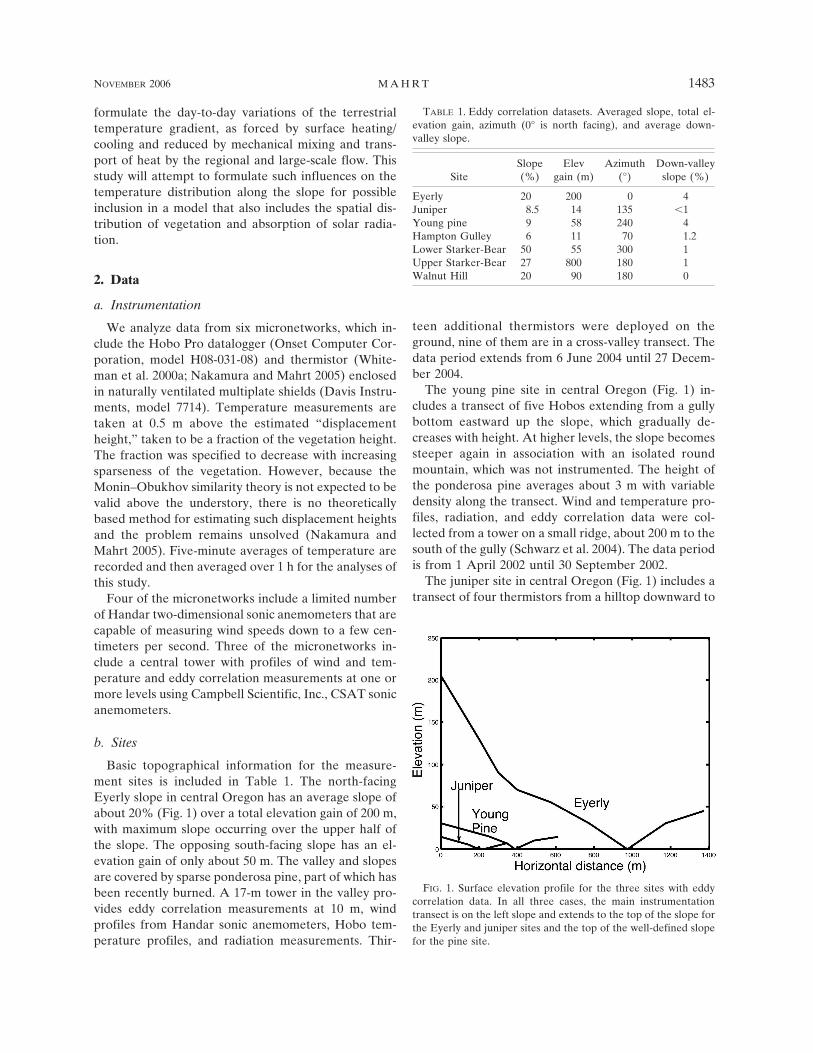
Because the Eyerly site is dry in summer, the surfaceheat flux increases systematically with increasing netradiation with only modest scatter. As a result of thestrong interrelationships between variables at this site,the daytime terrestrial temperature difference is highlycorrelated to the net radiation (Fig. 2). Inclusion ofinformation on the wind or friction velocity does not

improve the prediction of the terrestrial temperaturedifference for summer daytime conditions at this site.However, the close relationship between the daytimeterrestrial temperature difference and the net radiationneither extends to other seasons nor to other sites, par-ticularly when the surface latent heat flux reduces thesurface heating. For these other sites and seasons, thedaytime terrestrial temperature difference is moreclosely related to the thermal forcing * than net radia-tion.

For the Eyerly site, the daytime negative terrestrialtemperature difference increases approximately lin-early with increasing thermal forcing * [Eq. (2)] untilthe terrestrial potential temperature difference reachesa “saturation” value of about �1.5 K at a value of thethermal forcing of about 0.7 K (Fig. 3). The terrestrialtemperature gradient becomes independent of furtherincreases of the thermal forcing, though with substan-tial scatter. Apparently with sufficient heating, the ter-restrial temperature gradient becomes limited by con-vective mixing and redistribution of heat by the upval-ley and upslope circulations. We can therefore define amaximum or saturation value of the terrestrial tempera-ture gradient. For cases in the saturation regime, thefriction velocity tends to be proportional to the surfaceheat flux.

The large, positive values of the terrestrial tempera-ture gradient at the Eyerly site (red pluses, Fig. 3) areassociated with the early morning transition when theheat flux has become positive at the bottom of the slopebut the stratification along the north slope is still stable.

FIG. 2. Hourly values of the daytime terrestrial potential tem-perature difference (K) for the Eyerly site in summer as a functionof the net radiation. The normally clear skies and the discretiza-tion of net radiation into hourly averages leads to clumping of thenet radiation. Large positive values of the terrestrial temperaturedifference correspond to lingering stability during the early morn-ing transition (red �, 0500–0800 LST). A value of �1.1 K corre-sponds to well-mixed conditions (adiabatic lapse rate).

FIG. 3. Hourly values of the daytime terrestrial potential tem-perature difference for the Eyerly site in summer as a function ofthe thermal forcing * [Eq. (2)]. Red pluses identify observationsduring the morning transition period (0500–0800 LST). A value of�1.1 K corresponds to well-mixed conditions.


Fig 2 live 4/C Fig 3 live 4/C

For winter conditions at this site, the terrestrial tem-perature gradient does not reach saturation conditions,but within the range of winter values of * follows thesame dependence on * as in summer.

In contrast to the Eyerly site, the daytime surfacepotential temperature at the juniper and pine sites in-crease with surface elevation. Air temperatures at thepine site are warmer in areas with a sparse pine over-story as compared with absence of overstory at the bot-tom of the slope, corresponding to an increase of po-tential temperature with increasing surface elevation.Apparently the overstory is sufficiently sparse to allowfor significant heating of the surface, but reduces ven-tilation of the near surface air to allow more heatbuildup at the surface relative to open areas. The in-crease of temperature up the slope at the pine site couldbe underestimated by a few tenths of a degree becauseof the increase of overstory and decrease of radiativelyinduced thermistor errors up the slope (section 2c). Thepositive values of the daytime terrestrial potential tem-perature gradient at the pine and juniper sites increasewith thermal forcing up to a saturation value and thenbecome independent of the thermal forcing for largervalues. However, the relationship of the terrestrial tem-perature gradient to the thermal forcing at the juniperand pine sites is characterized by more scatter in com-parison with the larger slope at the Eyerly site. None-theless, saturation values were definable at the juniperand pine sites (Table 2, section 8).

b. Nocturnal temperature distribution

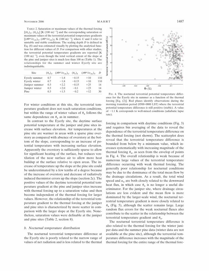
The nocturnal terrestrial temperature difference atthe Eyerly site is poorly related to the narrow range ofvalues of net radiation and is less related to the thermal

forcing in comparison with daytime conditions (Fig. 3)and requires bin averaging of the data to reveal thedependence of the terrestrial temperature difference onthe thermal forcing (not shown). The scatterplot doesreveal that the terrestrial temperature difference isbounded from below by a minimum value, which in-creases systematically with increasing magnitude of thethermal forcing *, as seen from the envelop of pointsin Fig. 4. The overall relationship is weak because ofnumerous large values of the terrestrial temperaturedifference occurring with weak thermal forcing. Thegenerally poor relationship for nocturnal conditionsmay be due to the dominance of the total mean flow bythe drainage circulations. As a result, the total windspeed and u* are both closely related to the downwardheat flux, in which case * is no longer a useful dis-criminator. For the juniper site, where drainage circu-lations are less evident and the mean flow is moredominated by the larger-scale wind, the nocturnal ter-restrial temperature gradient is more closely related to* (Fig. 5), although the scatter remains large. Largerandom flux errors for the weak nocturnal fluxes alsocontribute to the scatter in the relationship between theterrestrial temperature gradient and *.

The nocturnal terrestrial temperature difference isalso related to the thermal forcing for the winter juni-per data and the summer pine data (winter data are notavailable at the pine site), although the terrestrial tem-perature difference increases with the magnitude of thethermal forcing for the entire range of the thermal forc-

TABLE 2. Saturation or maximum values of the thermal forcing[(*)U, (*)S] [K (100 m)�1] and the corresponding saturation ormaximum values of the terrestrial potential temperature gradients[(�*/�zsfc)U, (�*/�zsfc)S; K (100 m)�1], where U and S refer tounstable and stable conditions. The scaling depth D is defined inEq. (8) and was estimated visually by plotting the analytical func-tion for different values of D. For comparison with other studies,the terrestrial potential temperature gradients are reported [K(100 m)�1], even though the total vertical extent of the slope atthe pine and juniper sites is much less than 100 m (Table 1). Therelationships for the summer and winter Eyerly site areindistinguishable.

Site (*)U (�*/�zsfc)U (*)S (�*/�zsfc)S D

Eyrely summer 0.7 �1.8 �0.15 �10 110Eyrely winter 0.7 �1.8 �0.15 �10 110Juniper summer 0.3 �2.2 �0.15 �25 14Juniper winter 0.3 �2.0 �0.1 �23 14Pine 0.3 �1.5 �0.2 �12 30

FIG. 4. The nocturnal terrestrial potential temperature differ-ence for the Eyerly site in summer as a function of the thermalforcing [Eq. (2)]. Red pluses identify observations during themorning transition period (0500–0800 LST) where the terrestrialpotential temperature difference is still positive (stable). A valueof �1.1 K corresponds to well-mixed conditions (adiabatic lapserate).


Fig 4 live 4/C

ing for both of these datasets. Because there is no rangeof thermal forcing where the terrestrial temperaturegradient becomes independent of the thermal forcingfor the pine and winter juniper sites, the nocturnalmaximum values of the terrestrial potential tempera-ture gradient are reported in Table 2 in place of thesaturation values in section 8.

A much smaller magnitude of the thermal forcing atnight generates a much larger magnitude of the terres-trial temperature gradient relative to daytime values.Weak downward nocturnal heat fluxes create greateralong-slope variations of air temperature in comparisonwith the large heat fluxes in the daytime when bothhorizontal and vertical mixing is greater.

The nocturnal terrestrial temperature gradient variesonly slowly with height for the lower half of the slope atthe Eyerly site (Fig. 6). The larger vertical gradient oftemperature on the tower above the valley floor rela-tive to the terrestrial temperature gradient correspondsto lower temperatures in the downslope flow relative tothe temperatures at the same level above the valley(Fig. 6). Whiteman (2000) and others have also foundthat the nocturnal terrestrial temperature gradient onsmall scales can be much smaller than the vertical tem-perature gradient away from the slope such that sur-faces of constant potential temperature tended to behorizontal over the valley and more parallel to theslope surface at the valley sidewalls. Similarly, the day-time unstable stratification above the valley floor ismuch larger than the negative terrestrial temperaturegradient at the Eyerly site (Fig. 7) so that the upslopeflow is warmer than the temperature at the same heightabove the valley floor.

5. Formulation of the dependence on the thermalforcing

Based on the concept of a saturation terrestrial tem-perature gradient, we formulate the terrestrial potentialtemperature gradient [Eq. (1)] to be a linear function ofthe thermal forcing up to the saturation value and con-

FIG. 6. Composited height distribution of the temperature forthe Eyerly site for late-evening conditions (0000–0400 LST) for a38-day period when the higher two temperature stations wereoperating. The red circles are the temperatures on the tower. Thesolid line is an adiabatic temperature profile corresponding towell-mixed conditions. The terrestrial temperature gradient sta-tistics reported in Table 2 are computed for the 960-m level andbelow where a longer dataset is available and the terrestrial tem-perature gradient is more constant.

FIG. 7. Composited height distribution of the temperature formidday (1100–1600 LST) at the Eyerly site. The red circles are thetemperatures on the tower. The solid line is an adiabatic tempera-ture profile. See Fig. 6 for additional explanation.

FIG. 5. The nocturnal terrestrial potential temperature differ-ence for the juniper site in summer as a function of the thermalforcing [Eq. (2)]. A value of �0.14 K corresponds to well-mixedconditions (adiabatic lapse rate).


Fig 5 6 7 live 4/C

stant for larger values. With this approach, f1(*) in Eq.(5) is formulated as

��*�zsfc

�U

�*��*�U

; 0 � �* � ��*�U

��*�zsfc

�S

�*��*�S

; ��*�S � �* � 0,�7�

where the subscript U refers to the saturation or maxi-mum value of the thermal forcing for daytime unstableconditions and the corresponding terrestrial potentialtemperature gradient at the bottom of the slope (z sfc →0). The subscript S refers to the values for nocturnalstable conditions. For magnitudes of the thermal forc-ing (*) greater than the saturation value, the terrestrialtemperature gradient is approximated as the saturationvalue, independent of the forcing value.

6. Height dependence of the terrestrialtemperature gradient

At the Eyerly site, the nocturnal terrestrial tempera-ture gradient at midslope decreases with height andreverses sign corresponding to a thermal belt where thetemperature reaches a maximum with respect to sur-face elevation (Fig. 6). For a greater variety of topo-graphical situations, we include data from the siteswithout eddy correlation data. The Walnut Hill site andthe Starker-Bear transect both include frequent datawith marine air penetration. To crudely filter outcloudy and windy days, which were not common in theother datasets, we use only days when the diurnal varia-tion exceeds the average diurnal variation. On the Wal-nut Hill slope, the nocturnal terrestrial temperaturegradient decreases with height to very small values atmidslope but does not reverse sign. Well-defined drain-age flow is also common on this slope. The terrestrialtemperature gradient decreases more gradually withsurface elevation when compared with the slopes at thepine, juniper, and Hampton Gulley sites. The total ver-tical extent of these slopes is below the relative heightof the thermal belt at the Eyerly site.

For a higher, more isolated mountain extending wellabove the surrounding terrain, the terrestrial tempera-ture gradient becomes smaller and more significantlyinfluenced by the background stratification of the freeair. This is illustrated with the higher part of our sitewith the largest vertical elevation change (Starker-Beartransect, section 2b). The nocturnal terrestrial tempera-ture gradient is large in the first few hundred metersabove the valley floor (Fig. 8) and is much smallerabove this level. This level is somewhat below the av-

eraged ridge top. The temperature at the second high-est site (square in Fig. 8) is probably cooler than thesurrounding area because it is in a gully on the northside of the slope. The height dependence of the terres-trial temperature gradient is more difficult to define inthe daytime, partly because it is smaller than the noc-turnal values and partly because it is more sensitive tochanges of vegetation and slope magnitude and aspect(section 8).

Based on the six micronetworks and the literature,the form of the height dependence of the terrestrialtemperature gradient is unique to every slope and de-pendent on the three-dimensionality of each slope. It isnot practical to define a different function, f2(z sfc /D),for every slope. Even at a given slope, f2(z sfc /D) ap-pears to vary diurnally and weakly with season. Re-stricting the formulation of the height dependence to asingle free parameter, the decrease of the terrestrialpotential temperature gradient with height is crudelyrepresented with an exponential decrease, such that

f �2�z�sfc �D� � exp��z�sfc �D��. �8�

The visual best-fit value of D, based on plotting thefunction with different values of D, appears to beroughly comparable to the height of the local ridgetops, although more sites are needed before such a con-clusion can be made with any confidence. Based on thecomposited vertical structure of the temperature, thevalue of D is chosen to be 110 m for the Eyerly site, theheight of the slope for the juniper site, and the approxi-mate height of the highest station for the pine site(Table 2). The exponential fit is a reasonable approxi-

FIG. 8. The averaged height distribution of surface air tempera-ture for the Starker-Bear micronetwork for summer at midnight.The black line is an adiabatic temperature profile. The squareindicates a station on the north-facing slope.


mation for the Walnut Hill site but is not a good fit forthe pine site or Starker-Bear site, where the upper partof the slope is above the surrounding ridges. Betterapproximations could be obtained with more complexfunctions with more than one free parameter.

7. Diurnal evolution

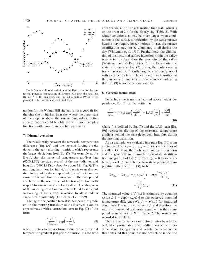
The relationship between the terrestrial temperaturedifference [Eq. (3)] and the thermal forcing breaksdown in the early morning transition, which representsthe largest deviations from Eq. (7). For example, at theEyerly site, the terrestrial temperature gradient lags(0700 LST) the sign reversal of the net radiation andheat flux (0500 LST) by about by about 2 h (Fig. 9). Themorning transition for individual days is even sharperthan indicated by the composited diurnal variation be-cause of the variation of sunrise within the data periodand because the occurrence of the transition time withrespect to sunrise varies between days. The sharpnessof the morning transition could be related to sufficientweakening of the surface inversion to allow suddenshear-driven instability (Lenschow et al. 1979).

The lag of the positive terrestrial temperature gradi-ent in the morning transition at the Eyerly site can beapproximated with a correction term to Eq. (7) of theform

� ��

�zsfc�

nexp��

�

�o�, �9�

where n refers to the nocturnal value of the terrestrialtemperature gradient just prior to sunrise, � is the time

after sunrise, and �o is the transition time scale, which ison the order of 2 h for the Eyerly site (Table 2). Withwinter conditions, �o may be much larger when elimi-nation of the surface stratification by the weak surfaceheating may require longer periods. In fact, the surfacestratification may not be eliminated at all during theday (Whiteman et al. 1999). Furthermore, the elimina-tion of the nocturnal surface inversion within the valleyis expected to depend on the geometry of the valley(Whiteman and McKee 1982). For the Eyerly site, thesystematic error in Eq. (7) during the early eveningtransition is not sufficiently large to confidently modelwith a correction term. The early morning transition atthe juniper and pine sites is more complex, indicatingthat Eq. (9) is not of general validity.

8. General formulation

To include the transition lag and above height de-pendence, Eq. (5) can be written as

��

�zsfc� f1��*� exp��z�sfc

D � � LAG� �

�o� �

��

�z,

�10�

where f1 is defined by Eq. (7) and the LAG term [Eq.(9)] represents the lag of the terrestrial temperaturegradient behind the time-dependent heat flux duringthe morning transition.

As an example, we vertically integrate Eq. (10) froma reference level (z � zref, z sfc � 0), such as the floor ofa valley. Omitting the early morning transition termand the generally much smaller basic-state stratifica-tion, integration of Eq. (10) from z sfc � 0 to some ar-bitrary level z predicts the terrestrial potential tem-perature difference [Eq. (3)] to be

��z�sfc� � ��zref� � f1��*�D�1 � exp��z�sfc

D ��

��

�z�z�sfc�. �11�

The saturated value of f1(*) is estimated by equatingf1(*) D[1 � exp(�z sfc /D)] to the observed potentialtemperature difference (z sfc) � (zref) for saturatedconditions. The saturated value of f1, and therefore thesaturated terrestrial temperature gradient, is then com-puted from values of D in Table 2. The results arerecorded in Table 2.

The parameter values vary between sites by a factorof 2, which presumably reflects differences of the three-dimensional topography and vegetation between thethree sites. At this point, it is not possible to model the

FIG. 9. Summer diurnal variation at the Eyerly site for the ter-restrial potential temperature difference (K, stars), the heat flux(K m s�1 � 10, triangles), and the net radiation (W m�2/100;pluses) for the conditionally selected days.


variation of the saturation values between sites. To fur-ther study the difference between sites, we include thenoneddy correlations sites, again using only days wherethe diurnal temperature variation was greater than theseasonal average diurnal variation. The nocturnal ter-restrial temperature gradients were largest at the bot-tom of the Starker-Bear transect, Hampton Gully, andjuniper site, all of which area valley sites with a weakdown-valley slope. The terrestrial temperature gradientwas about half as large at the Eyerly site where thedown-valley slope was greater and the opposing slopelength is only about 15% of the north-facing slope. Thenocturnal terrestrial temperature gradient is weakest atthe pine site, where the opposing slope was muchshorter and the down-valley slope was significant(Table 1), and at Walnut Hill, where there was no op-posing slope. Magono et al. (1982) attributed extremelycold temperatures at the surface of a basin to a lack ofdown-valley flow.

Slope aspect and vegetation

The above prediction of the terrestrial temperaturegradient for daytime conditions may require adjust-ment for the influence of slope aspect and vegetation.Such adjustments cannot be tied to the height depen-dence of the terrestrial temperature and an indepen-dent term is required, such that

��z� � ��z�F � G��*, M, A�, �12�

where (z)F is the value of the potential temperaturepredicted by Eq. (11) and G(*, M, A) represents theinfluence of slope aspect on incident solar radiation,magnitude and curvature of the terrain, and vegetation.Here G is expected to increase with the thermal forcing* because spatial variations of surface air temperatureare expected to be largest with greater surface heatingand less mixing and horizontal transport. The influenceof spatial variations of incident solar radiation and LAIof the overstory has been included in Moore et al.(1993) and Bellasio et al. (2005).

In our datasets, the influence of the spatial variationof the incident solar radiation on the surface air tem-perature was definable but complicated by several ad-ditional influences. The effect of spatial variation of theincident solar radiation on the air temperature distri-bution is not only related to the thermal forcing but ismuch greater in the early morning when the mixingdepth is small. At this time, the impact of differentialsurface heating is confined to a thin layer and has agreater impact on the air temperature distribution. Inaddition, south-facing slopes at our semiarid forestedsites are characterized by less overstory and drier soil in

comparison with the north-facing slopes. Consequently,the effects of slope aspect and vegetation are difficult toseparate. Last, the impact of surface variations aregreater when the horizontal scale of such variations aregreater so that their impact is less vulnerable to reduc-tion by atmospheric mixing (their blending height ishigher).

9. Conclusions

The above analysis of temperature data from threedifferent micronetworks with eddy correlation data incomplex terrain indicates that the magnitude of thealong-slope variation of the surface potential tempera-ture with surface elevation (terrestrial potential tem-perature gradient) increases approximately linearlywith increasing surface heating or cooling. The magni-tude of the terrestrial temperature gradient decreaseswith increasing mechanical redistribution of heat result-ing from vertical mixing and horizontal transport.

For a given site, the magnitude of the daytime ter-restrial temperature gradient is reasonably well pre-dicted by a thermal forcing temperature scale * [Eq.(2)], defined as the ratio of the surface heat flux to thesurface friction velocity. When the thermal forcing (*)exceeds a saturation value, the terrestrial temperaturegradient becomes independent of the forcing. Appar-ently, mixing and redistribution of heat by slope-generated circulations lead to a maximum or saturationvalue of the terrestrial temperature gradient for a givensite. In the saturation regime, the flow appears to bedominated by slope circulations and u* is proportionalto the surface heat flux. However, the saturation valueof the terrestrial temperature gradient varies substan-tially between sites and is sometimes never reached inwinter. The sign of the smaller daytime terrestrial tem-perature gradient may be negative or positive, depend-ing on the details of the topography and height distri-bution of vegetation.

For nocturnal conditions, the terrestrial temperaturegradient becomes poorly related to * for the Eyerlysite, where the mean flow and friction velocity aredominated by the local thermally driven circulations,which in turn are proportional to the magnitude of thedownward heat flux. Use of multiple velocity scalesmay improve the relationship for this site, although thepresent datasets are inadequate for construction ofmore complex relationships. The temperature scale *is a better predictor for the other sites. The nocturnalterrestrial temperature gradient is greater on the sideslopes of valleys with weaker down-valley slope, allow-ing buildup of cold air at the base of the slope. Exposedslopes on isolated hills have a smaller terrestrial tem-


perature gradient relative to those of the valley sideslopes.

Equation (11) quantitatively represents the impor-tance of the influence of mixing and slopes circulationson the terrestrial temperature gradient. This represen-tation performs well at our sites in summer where thesynoptic situation and diurnal cycle normally vary littlebetween days. The generality of this approach is notknown, and presumably its performance would degradeat locations with significant synoptic variability. Thepresent approach does not work well during the earlymorning transition period when the surface inversionmay survive well after the surface heat flux becomespositive. This approach does not include a general pro-cedure for predicting the large variations of coefficientsbetween different topographical situations. Toward thisgoal, the above formulation for the influence of mixingon the terrestrial temperature gradient needs to becombined with a model of the influences of slope ori-entation and vegetation on radiative forcing (section8a). Without such a generalization, the practical use ofour formulation is probably limited.

Acknowledgments. I gratefully acknowledge the veryhelpful comments of David Whiteman and RobertoBellasio and greatly appreciate the useful comments ofboth reviewers. I also appreciate the deployment andmeasurement collection by John Wong at the Eyerlyand pine sites and the data processing of Dean Vickers.William Tahnk and Kayge McNab assisted with the col-lection of temperature data on the Starker-Bear Trail.This material is based upon work supported by Con-tract W911NF-05-C-0067 from the Army Research Of-fice and Grant 0107617-ATM from the Physical Meteo-rology Program of the National Sciences Program.

REFERENCES

Acevedo, O. C., and D. R. Fitzjarrald, 2001: The early eveningsurface-layer transition: Temporal and spatial variability. J.Atmos. Sci., 58, 2650–2667.

Bellasio, R., G. Maffeis, J. S. Scire, M. G. Longoni, R. Bianconi,and N. Quaranta, 2005: Algorithms to account for topo-graphic shading effects and surface temperature dependenceon terrain elevation in diagnostic meteorological models.Bound.-Layer Meteor., 114, 595–614.

Bootsma, A., 1976: Estimating minimum temperature and clima-tological freeze risk in hilly terrain. Agric. For. Meteor., 16,425–443.

Chung, U., and J. I. Yun, 2004: Solar irradiance-corrected spatialinterpolation of hourly temperatures in complex terrain. Ag-ric. For. Meteor., 126, 129–140.

Clements, C. B., C. D. Whiteman, and J. D. Horel, 2003: Cold-air-pool structure and evolution in a mountain basin: Peter Sinks,Utah. J. Appl. Meteor., 42, 752–768.

Daly, C., W. Gibson, G. Taylor, G. Johnson, and P. Pasteris, 2002:

A knowledge-based approach to the statistical mapping ofclimate. Climate Res., 22, 99–113.

Doran, J. C., and T. W. Horst, 1983: Observations and models ofsimple nocturnal slope flows. J. Atmos. Sci., 40, 708–717.

——, and S. Zhong, 1994: Regional drainage flows in the PacificNorthwest. Mon. Wea. Rev., 122, 1158–1167.

Gustavsson, T., M. Karlsson, J. Bogren, and S. Sindqvist, 1998:Development of temperature patterns during clear nights. J.Appl. Meteor., 37, 559–571.

Haiden, T., and C. D. Whiteman, 2005: Katabatic flow mecha-nisms on a low-angle slope. J. Appl. Meteor., 44, 113–126.

Heywood, G. S. P., 1933: Katabatic winds in a valley. Quart. J.Roy. Meteor. Soc., 59, 43–57.

Hocevar, A., and J. D. Martsolf, 1971: Temperature distributionunder radiation frost conditions in a central Pennsylvaniavalley. Agric. For. Meteor., 8, 371–383.

Kimura, F., and T. Kuwagata, 1993: Thermally induced wind pass-ing from plain to basin over a mountain range. J. Appl. Me-teor., 32, 1538–1547.

Kurita, H., H. Ueda, and S. Mitsumoto, 1990: Combination oflocal wind systems under light gradient wind conditions andits contribution to the long-range transport of air pollutants.J. Appl. Meteor., 29, 331–348.

LeMone, M. A., K. I. Ikeda, R. L. Grossman, and M. W. Rotach,2003: Horizontal variability of 2-m temperature at night dur-ing CASES-97. J. Atmos. Sci., 60, 2431–2449.

Lenschow, D. H., B. B. Stankov, and L. Mahrt, 1979: The rapidmorning boundary-layer transition. J. Atmos. Sci., 36, 2108–2124.

Liston, G. E., R. A. Pielke Sr., and E. M. Greene, 1999: Improvingfirst-order snow-related deficiencies in a regional climatemodel. J. Geophys. Res., 104, 19 559–19 567.

Magono, C., C. Nakamura, and Y. Yoshida, 1982: Nocturnal cool-ing of the Moshiri Basin, Hokkaido in midwinter. J. Meteor.Soc. Japan, 60, 1106–1116.

Mahrt, L., and R. Heald, 1983: Nocturnal surface temperaturedistribution as remotely sensed from low-flying aircraft. Ag-ric. For. Meteor., 28, 99–107.

——, and D. Vickers, 2005: Boundary-layer adjustment oversmall-scale changes of surface heat flux. Bound.-Layer Me-teor., 116, 313–330.

——, ——, R. Nakamura, J. Sun, S. Burns, D. Lenschow, and M.Soler, 2001: Shallow drainage and gully flows. Bound.-LayerMeteor., 101, 243–260.

Moore, I. D., T. W. Norton, and J. E. Williams, 1993: Modellingenvironmental heterogeneity in forested landscapes. J. Hy-drol., 150, 717–747.

Nakamura, R., and L. Mahrt, 2005: Air temperature measurementerrors in naturally ventilated radiation shields. J. Atmos. Oce-anic Technol., 22, 1046–1058.

Nie, D., T. Demetriades-Shah, and E. T. Kanemasu, 1992: Surfaceenergy fluxes on four slope sites during FIFE 1988. J. Geo-phys. Res., 97, 18 641–18 649.

Pielke, R. A., and P. Mehring, 1977: Use of mesoscale climatologyin mountainous terrain to improve the spatial representationof mean monthly temperatures. Mon. Wea. Rev., 105, 108–112.

Richardson, A. D., X. Lee, and A. J. Friedland, 2004: Microcli-matology of treeline spruce-fir forests in mountains of thenortheastern United States. Agric. For. Meteor., 125, 53–66.

Schwarz, P. A., B. E. Law, M. Williams, J. Irvine, M. Kurpius, andD. Moore, 2004: Climatic versus biotic constraints on carbonand water fluxes in seasonally drought-affected ponderosa


pine ecosystems. Global Biogeochem. Cycles, 18, GB4007,doi:10.1029/2004GB002234.

Stewart, J. Q., C. D. Whiteman, W. J. Steenburgh, and X. Bian,2002: A climatological study of thermally driven wind sys-tems of the U.S. intermountain West. Bull. Amer. Meteor.Soc., 83, 699–708.

Tabony, R. C., 1985: Relations between minimum temperatureand topography in Great Britain. J. Climatol., 5, 503–520.

Thorton, P., S. Running, and M. White, 1997: Generating surfacesof daily meteorological variables over large regions of com-plex terrain. J. Hydrol., 190, 214–251.

Vickers, D., and L. Mahrt, 1997: Quality control and flux samplingproblems for tower and aircraft data. J. Atmos. Oceanic Tech-nol., 14, 512–526.

——, and ——, 2006: A solution for flux contamination by meso-scale motions with very weak turbulence. Bound.-Layer Me-teor., 118, 431–447.

Whiteman, C. D., 2000: Mountain Meteorology. Oxford Univer-sity Press, 355 pp.

——, and T. B. McKee, 1982: Breakup of temperature inversions

in deep mountain valleys. Part II: Thermodynamic model. J.Appl. Meteor., 21, 290–302.

——, K. J. Allwine, L. J. Fritschen, M. M. Orgill, and J. R. Simp-son, 1989: Deep valley radiation and surface energy budgetmicroclimates. Part II: Energy budget. J. Appl. Meteor., 28,427–437.

——, X. Bian, and S. Zhong, 1999: Wintertime evolution of thetemperature inversion in the Colorado plateau basin. J. Appl.Meteor., 38, 1103–1117.

——, J. Hubbe, and W. Shaw, 2000a: Evaluation of an inexpensivetemperature data logger for meteorological applications. J.Atmos. Oceanic Technol., 17, 77–81.

——, S. Zhong, X. Bian, J. D. Fast, and J. C. Doran, 2000b:Boundary layer evolution and regional-scale diurnal circula-tions over the Mexico basin and Mexican plateau. J. Geo-phys. Res., 105, 10 081–10 102.

Yoshino, M. M., 1975: Climate in a Small Area. Tokyo Press, 549pp.

——, 1984: Thermal belt and cold air drainage on the mountainslope and cold air lake in the basin at quiet clear night. Geo.J., 8, 235–250.


Documents

Variation of Surface Air Temperature in Complex Terrain