1

Variation in the Value of Travel Time Savings

and its Impact on the Benefits of Managed Lanes

Sunil Patil, Analyst

RAND Europe Westbrook Center, Milton Road

Cambridge, UK-CB4 1YG Phone: +44-1223-353-329

spatil@rand.org

Mark Burris,* E. B. Snead I Associate Professor

Zachry Department of Civil Engineering Texas A&M University

CE/TTI Building, Room No.304-C College Station, Texas-77843-3136

Phone: 979-845-9875 Fax: 979-845-6481 mburris@tamu.edu

Douglass Shaw, Professor

Department of Agricultural Economics and Research Fellow, Hazard Reduction and Recovery Center

Texas A&M University Blocker Building, Room No.308F

College Station, Texas-77843-2124 wdshaw@ag.tamu.edu

Sisinnio Concas,

Senior Research Associate Center for Urban Transportation Research

4202 E. Fowler Avenue, CUT 100 University of South Florida

concas@cutr.usf.edu *Corresponding Author

Keywords: Value of travel time savings, managed lanes, urgent situations, mixed logit model

2

ABSTRACT

This research examines the variation in the value of travel time savings (VTTS) for

travelers with a managed lane (ML) option when taking an ordinary trip versus a trip that is

unusual in some way. VTTS estimates vary substantially depending on the urgency of the trip

made. At the low end, the mean VTTS for a traveler who wants to make extra stops and still

arrive on time is approximately 10 percent higher than that for an ordinary trip. At the high end,

a traveler running late for an appointment shows a mean VTTS that is approximately 300 percent

higher than that for an ordinary trip. These estimates vary widely over the population of

travelers. In light of these variations, the value of an uncongested travel alternative (such as

MLs) is examined and found to be greatly undervalued if using typical VTTS estimates.

3

1. INTRODUCTION

Managed lanes (MLs) generally offer travelers a tolled, congestion-free, alternative to a

congested, but toll-free, route. Studying travelers’ willingness to pay for this uncongested

alternative offers transportation planners a unique opportunity to better understand how travelers

value their travel time savings under different circumstances. This research examines the

variation in the value of travel time savings (VTTS) for travelers with a ML option when taking

an ordinary trip versus a trip that is unusual in some way. We hypothesize that the VTTS for an

unusual trip, such as when running late for a meeting, would be much higher than the VTTS on

an ordinary trip. If true, the uncongested travel alternatives (such as MLs) would be greatly

undervalued if the estimate of VTTS for ordinary trips is used in a cost-benefit analysis.

This variability in VTTS is further supported by previous research indicating that

travelers’ VTTS changes depending on the time of day the trip is taken (Small et al., 1999; Tseng

and Verhoef, 2008) and whether the traveler was delayed (Tilahun and Levinson, 2008).

Additionally, typical stated preference (SP) studies designed for VTTS estimation for MLs

travelers tend to underestimate VTTS compared to studies that use the revealed preference

approach (see Ghosh, 2001; Brownstone et al., 2003, Brownstone and Small, 2005).1 Further,

many of the studies of existing managed lanes have concluded that the vast majority of travelers

use MLs only occasionally, and include travelers from all income groups (Sullivan et al., 2000;

1 Revealed preference uses data on actual trips taken and actual tolls paid, if any tolls exist. Conversely, “stated”

preference modeling constructs choices of trips as a function of attributes that the investigator designs and builds

into the modeling exercise. The stated choice approach allows exploration of responses to tolls that may not exist in

the transportation system.

4

Collier and Goodin, 2002; Burris and Stockton, 2004). These findings indicate that travelers are

assigning different values to their travel time savings on different trip occasions and using MLs

when those VTTS are in the higher end of the travelers’ range of VTTS.

This research takes advantage of the recently opened Katy Freeway MLs, Houston,

Texas, to estimate the range of VTTS, and its impact on the use of MLs. Section 2 describes the

implementation of a SP survey of the Katy Freeway travelers, which was undertaken as part of

the research. Section 3 describes the analysis technique used to extract the travelers’ range of

VTTS in ordinary and unusual trip situations from the survey data. Section 4 includes the VTTS

results and a discussion of how these can be used to better understand traveler decisions on MLs

facilities and how to measure the true benefits offered by MLs. Section 5 offers conclusions

about this research.

2. SURVEY DESIGN AND DATA COLLECTION

2.1 Study Location

Houston, Texas is one of the largest cities in the United States with a 2007 US Census

population estimate of over 5.7 million people living in the Houston metropolitan area (USCB,

2007). The city has an extensive network of freeways which includes the Katy Freeway; a 23-

mile stretch of Interstate-10 connecting the cities of Katy and Houston (Figure 1). An expansion

project for this freeway began in 2003 and the expanded facility first opened in October 2008

(TxDOT, 2009). The new facility also has two Katy Tollway/Managed Lanes (MLs) in each

direction between State Highway 6 and Interstate 610 (a distance of 12 miles). METRO buses

and high occupancy vehicles (HOV2+ with 2 or more people in a vehicle) and motorcycles can

use the MLs for free during peak hours (Monday to Friday 5 a.m. to 11 a.m. and 2 p.m. to 8

5

p.m.). Beginning in April 2009, single occupant vehicle drivers willing to pay a toll could also

use the MLs while HOVs and motorcycles continue to use the lanes toll-free during the peak

hours and pay a toll only during off-peak hours. The toll must be paid electronically, using

EZTag or TxTag (HCTRA, 2009), the local electronic tags that allow passage through toll gates

without stopping to pay by cash or credit card. Tolls on this new facility vary by the time of day

($4, $2, $1 for peak, shoulder and off-peak times respectively for the 12 mile stretch).

As part of this research, a SP survey of Katy Freeway travelers was conducted just after

the Katy Freeway MLs opened in October 2008. This allowed survey respondents to be familiar

with the facility and most of the choice alternatives offered in the survey.

2.2 Data collection

Survey responses were collected via an interne-based survey the internet. Due to its

online nature, the sampling process presents a potential sampling bias as it requires the sample

individuals to have at least some temporary, if not permanent, internet access in order to take the

survey. We conducted a detailed sampling bias analysis and found that the sample used in the

current study is similar to that obtained from a survey of travelers observed using the Katy

Freeway. The discussion of sampling issues for internet based surveys in general and the analysis

of sampling bias for this study are presented in Patil et al. (forthcoming, 2011) and Burris and

Patil (2009).

A total of 6,312 respondents took at least some portion of the online/internet survey. Of

these, 3,990 respondents fully completed the survey. We removed 973 responses due to a

problem in the implementation of a particular SP design strategy (see Patil et al. 2011 for

details), and 119 responses from motorcycle and transit travelers. The final sample considered

6

for model estimation consists of a total 2,898 respondents who answered the questions as

discussed in the next section of this paper.

2.3 Details of the Survey Questionnaire

Each respondent was presented with the SP survey, which took approximately 12 to 15

minutes to complete. The survey questionnaire was structured to first ask the respondent

questions about their most recent trip on the Katy Freeway, followed by an introduction to the

managed lanes concept was provided. Next there were questions regarding the respondent’s

attitudes towards this ML concept, a set SP questions, and key socio-economic questions that can

potentially be used to explain the choices.

In the fifth section of the survey questionnaire respondents were presented with three

pairs of SP questions, which were randomly assigned to the respondent based on the prior week

trip characteristics provided in the first part of the questionnaire. Each pair of SP questions asked

about mode choice under an ordinary situation and an urgent situation. The respondent could

choose from among four alternatives that feature different modes of travel, and other key

attributes of the alternatives. The specific values of travel time and toll to be presented in the SP

questions were calculated using the reported actual trip length for each respondent and using one

of the three underlying experimental designs. The designs included random, adaptive random,

and D-Efficient design. A detailed discussion regarding how design impacted results is included

in Patil et al. (forthcoming, 2011). In each SP question pair, the respondents were presented with

four out of following five travel modes as labeled alternatives.

1. Carpool on general purpose lanes (CP-GPL),

2. Drive alone on general purpose lanes (DA-GPL),

7

3. Drive alone on managed lanes (DA-ML),

4. Carpool with one other person on managed lanes (HOV2-ML),

5. Carpool with three or more people on managed lanes (HOV3+-ML).

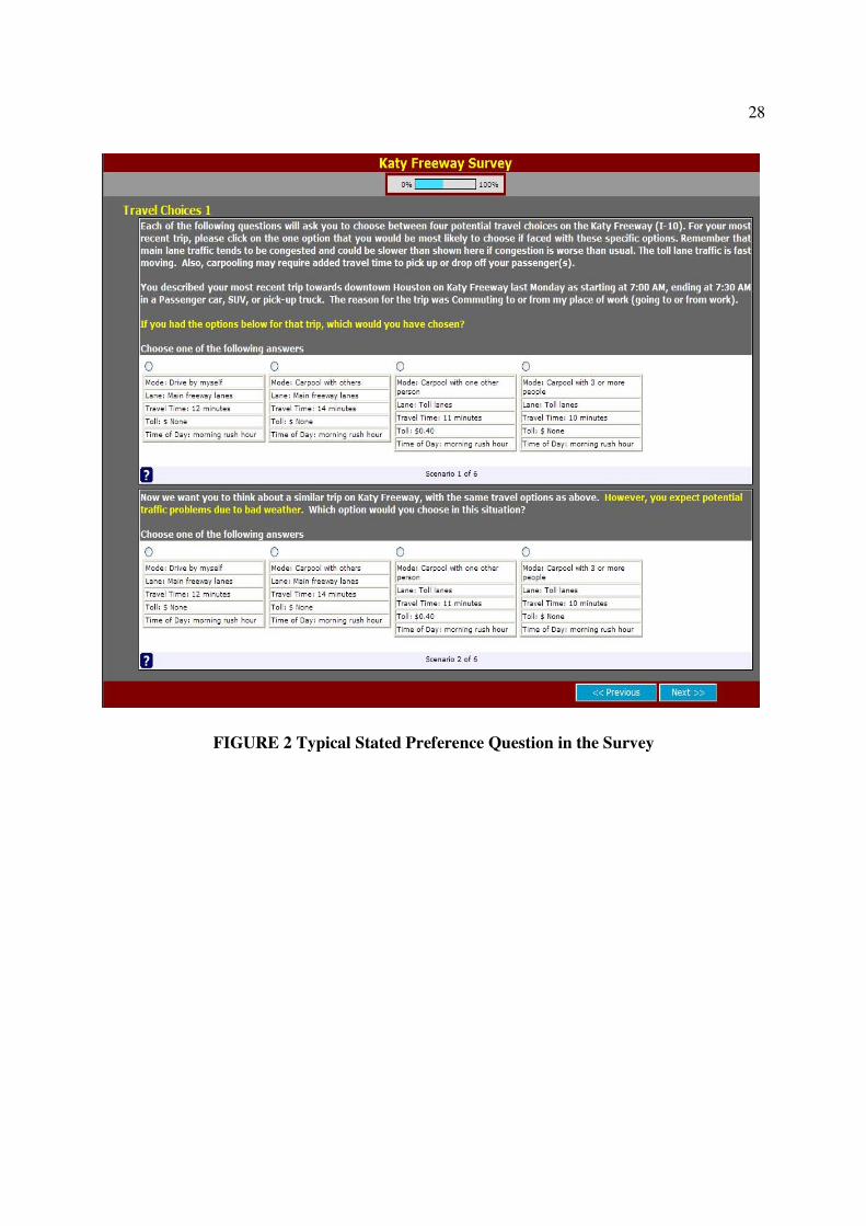
A typical presentation of a pair of SP questions presented in the survey questionnaire is

shown in Figure 2.

2.4 Details of Urgent Situations Presented

One of the main objectives of this study was to investigate if travelers value their time

differently when faced by an urgent travel situation versus an ordinary travel situation. The SP

questions were designed to capture the possible difference in VTTS for an individual’s ordinary

and urgent trip situations. In all the three SP question pairs, one of six categories was used to

describe the urgent trip situation that a traveler can face, while the ordinary trip referred to the

typical trip in the week prior to the time the survey was taken. The six urgent reasons and their

implications are given in Table 1. The wording of the urgent trip situation categories and

descriptions were considered in an attempt to make them:

• applicable to numerous other urgent trip situations that may also fall into that

category,

• applicable to either direction of travel (towards/away from downtown),

• applicable to all days of the week (weekday/weekend), and

• applicable to all times of departure (peak/shoulder /off-peak).

Note that not all of the urgent trip situations in Table 1 occur unexpectedly as some of them can

be known and planned for in advance. In all six urgent trip situations the hypothesis was that

travelers’ VTTS would be higher than it is for travel in ordinary trip situations. In each pair of SP

8

questions, the travel time and toll values used for the question relating to an urgent trip situation

were the same as those corresponding to the ordinary travel situation. A description of the

discrete choice model used to analyze these respondent’s mode choices and estimate their VTTS

in ordinary and urgent travel situations is presented in the next section.

3. EMPIRICAL DESIGN

The standard conditional multinomial logit model (MNL) is the most popular form of

discrete choice model in which the utility of an alternative j =1,...,J for an individual q = 1,..,Q in

a choice situation t =1,…,T as specified by

U,, x ,, (1)

where, = the coefficients to be estimated,

x = the (K 1) vector of K independent variables which include alternative specific

constants, characteristics of the individuals, characteristics of the alternative and

other descriptive variables affecting the choice.

,, = the error components which may be due unaccounted measurement error,

correlation in the parameters, unobserved individual preferences and other similar

unobserved characteristics of the choice making

The model consists of a deterministic part and a random (error) component, where the

randomness is introduced by the investigator rather and not by an individual’s uncertainty about

an outcome. The error component (,,) is assumed to be identical and independently

distributed (iid) Type 1 extreme value, which gives a closed form multinomial logit model

probability (Equation 2). This assumption yields very simple properties, but it makes the MNL

9

unable to account for individual heterogeneity, a shortcoming stemming from the independence

from irrelevant alternatives (IIA) property.

Prob choice j |individual q, XXXXq,t,choice setting t* +,-./x0123

∑ +,-./x0123560=1

(2)

To assess these limitations, mixed logit (or random parameter logit- RPL) models are

now frequently being used in empirical work (Train, 1998; Revelt and Train, 1998; Train, 2003).

Thanks to increased computational power, the mixed logit model has evolved from a basic

specification, which allows only the parameters to be distributed randomly, to more sophisticated

specifications that can accommodate repeated responses from the same individual (as panel data

or autocorrelation), scale differences in data sources, different error structures,

heteroscedasticity, and also heterogeneity in preferences, which may arise from various sources

(see, Brownstone and Train, 1999; Ben-Akiva et al., 2001; Bhat and Castelar, 2002; Greene et

al., 2006; Greene and Hensher, 2007; Hensher et al., 2008). The equations below follow the

notation and the specification used for the more flexible models, as discussed in Greene and

Hensher (2007) and show the expansion from a basic mixed logit specification to the more

advanced one applied in this study is explained next.

The simplest specification of the mixed logit allows the parameters to be distributed

randomly to account for individuals’ heterogeneity in taste and attributes. The analyst chooses a

probability distribution that is assumed to be appropriate for the taste parameter, typically a

normal, lognormal, or a triangular distribution. Each estimated parameter can thus be assumed to

vary across individuals or

78 798 :8;8 (3)

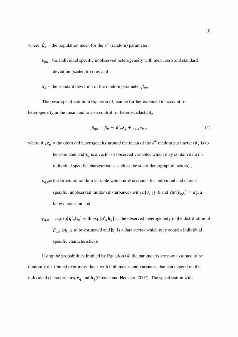
10

where, 798 = the population mean for the kth (random) parameter,

;8= the individual specific unobserved heterogeneity with mean zero and standard

deviation (scaled to) one, and

:8 = the standard deviation of the random parameter 78.

The basic specification in Equation (3) can be further extended to account for

heterogeneity in the mean and to also control for heteroscedasticity

78 798 <8= >,8;,8 (4)

where <8= = the observed heterogeneity around the mean of the kth random parameter (<8 is to

be estimated and zzzz is a vector of observed variables which may contain data on

individual specific characteristics such as the socio-demographic factors) ,

;,8= the structural random variable which now accounts for individual and choice

specific, unobserved random disturbances with E[;,8]=0 and VarA;,8B C8D, a

known constant and

>,8 :8expAG8HB with expAG8HB as the observed heterogeneity in the distribution of

7,8 (G8 is to be estimated and hhhh is a data vector which may contain individual

specific characteristics).

Using the probabilities implied by Equation (4) the parameters are now assumed to be

randomly distributed over individuals with both means and variances that can depend on the

individual characteristics, zzzz and H(Greene and Hensher, 2007). The specification with

11

heterogeneity around the mean can be applied to the problem of estimating the VTTS for

different groups of individuals.

Following Hensher et al. (2005, p. 660-667), we investigate preference heterogeneity

around the mean of travel time and toll parameters for the ordinary and six urgent travel

situations. To produce estimation results that are behaviorally meaningful, we assume a

constrained triangular distribution for the travel time coefficient (7IJK) with its spread equal to

the mean, i.e. √6 N :IJK= 79IJK (see Train (2003) for a discussion of the details of the triangular

distribution). However, the toll coefficient (7O) is assumed to be fixed (non-random) to facilitate

the VTTS estimation. Note that, both the time and toll parameters are estimated in a way that

does take into account heterogeneity in preferences that may arise because of the six urgent trip

situations. Next, two dummy variables for medium and high household income groups are added

to the model specification in order to capture the observable heterogeneity in the toll parameter

with respect to three income categories (low, medium and high income). Equations 5 and 6

specify the parameters for the time (7IJK* and toll (7O* (shown here without heteroscedasticity

and without individual specific notation q for ease of presentation). These equations are

essentially marginal utilities with respect to time and cost (i.e. partial derivatives of the utility

function with respect to time and cost).

7IJK 79IJK PQ ImpAppt PD LateAppt PV WorryTime PZ BadWeather

P\ LateML P^ ExtraStops 79IJK aIJK (5)

7O 79O PQO ImpAppt PDO bCacAppt PVO WorryTime PZO BadWeather

P\O LateML P^O ExtraStops PdO efghci PjO IncHigh (6)

12

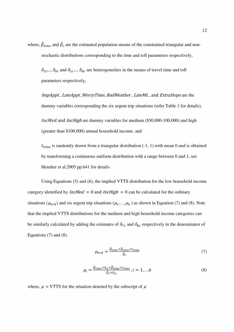
where, 79IJK and 79O are the estimated population means of the constrained triangular and non-

stochastic distributions corresponding to the time and toll parameters respectively,

PQ,.., P^ and PQO,.., PjO are heterogeneities in the means of travel time and toll

parameters respectively,

ImpAppt , LateAppt ,WorryTime, BadWeather , LateML , and ExtraStops are the

dummy variables corresponding the six urgent trip situations (refer Table 1 for details),

efghci and IncHigh are dummy variables for medium ($50,000-100,000) and high

(greater than $100,000) annual household income, and

aIJK is randomly drawn from a triangular distribution (-1, 1) with mean 0 and is obtained

by transforming a continuous uniform distribution with a range between 0 and 1, see

Hensher et al.2005 pp.641 for details.

Using Equations (5) and (6), the implied VTTS distribution for the low household income

category identified by IncMed 0 and IncHigh 0 can be calculated for the ordinary

situations (µnop) and six urgent trip situations (µQ, . . , µ^ ) as shown in Equation (7) and (8). Note

that the implied VTTS distributions for the medium and high household income categories can

be similarly calculated by adding the estimates of PdO and PjO respectively in the denominator of

Equations (7) and (8).

µnop rs26tuvrs26tu 26tu

rsw (7)

µI rs26tuvx62vrs26tu 26tu

rswvx6w, y 1, . . ,6 (8)

where, µ = VTTS for the situation denoted by the subscript of µ

13

Further extension of the mixed logit model can account for autocorrelation that may exist

in panel data or repeated choice situations. Thus the preferences as estimated by the random

parameters are allowed to evolve over time or over sequence of choices (Greene and Hensher,

2007). The underlying structural parameter, ;,8 in Equation 4 is then specified for each situation

t as

z,8, 8z,8,|Q ,8,, (9)

where, 8 = the autocorrelation parameters that are to be estimated

,8, = the new underlying structural random variable.

While the above extensions (Equations 4 and 8) are related solely to the random

parameters (not to the error components), further modifications to the model specification can be

made to incorporate additional unobserved heterogeneity through effects that are associated with

the preferences within the alternatives. For example, Equation 10 shows the individual’s utility

function with an extension yielding the ‘kernel logit’ model (Brownstone and Train, 1999; Ben-

Akiva et al., 2001; Greene and Hensher, 2007 for details)

U,, x,, ,, ∑ gJW,J~J=1 , (10)

where gJ 1 if the error component m appears in the utility function of alternative j and

W,J= the normally distributed effects with zero mean.

The effects,W,J are associated with individual preferences within the choices (alternatives) and

can account for unobserved heterogeneity such that

14

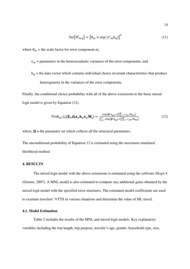
VarWJ, J exp τh*D (11)

where J = the scale factor for error component m,

J = parameters in the heteroscedastic variances of the error components, and

h = the data vector which contains individual choice invariant characteristics that produce

heterogeneity in the variances of the error components.

Finally, the conditional choice probability with all of the above extensions to the basic mixed

logit model is given by Equation (12).

Prob,jt|XXXXit,ΩΩΩΩ,zzzzq,hhhhq,vvvvq,WWWWq* +,-./x012v∑ O1tWt0

t=1 3

∑ +,-./x012v∑ O1tWt0t=1 35

1=1 (12)

where, ΩΩΩΩ = the parameter set which collects all the structural parameters.

The unconditional probability of Equation 12 is estimated using the maximum simulated

likelihood method.

4. RESULTS

The mixed logit model with the above extensions is estimated using the software Nlogit 4

(Greene, 2007). A MNL model is also estimated to compare any additional gains obtained by the

mixed logit model with the specified error structures. The estimated model coefficients are used

to examine travelers’ VTTS in various situations and determine the value of ML travel.

4.1. Model Estimation

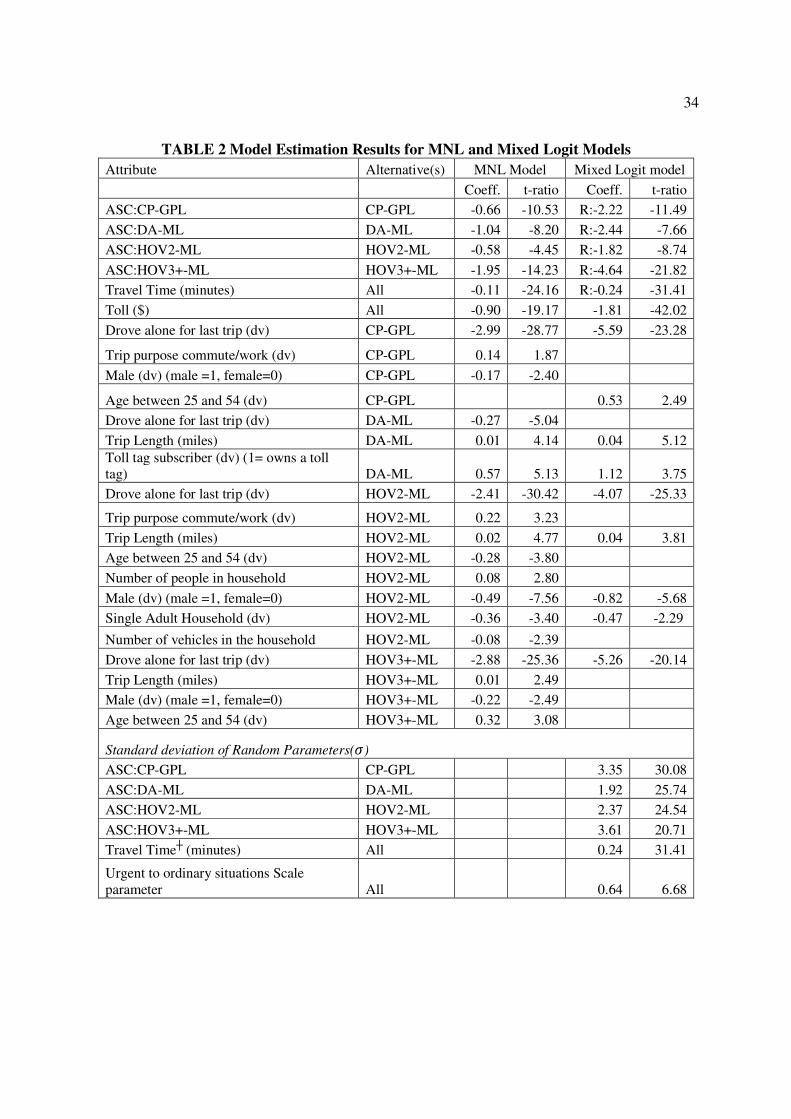
Table 2 includes the results of the MNL and mixed logit models. Key explanatory

variables including the trip length, trip purpose, traveler’s age, gender, household type, size,

15

vehicle stock, and vehicle occupancy for the individual’s most recent trip were found to be

significant in the basic model (see, Burris and Patil 2009 for a more detailed discussion of all

parameters and variables).

The mixed logit model estimation procedure uses 350 Halton draws to minimize

simulation variance. The estimation procedure used here utilized 350 Halton draws2 primarily

because use of more draws takes multiple days for estimation of this complex model. Note that

previous studies have concluded that the use of Halton sequences rather than random draws

decreases the total estimation time, which can be extensive in complex models, and smoothes the

simulation (Bhat, 2001, Train, 2003). It is also common to use 200 to 500 Halton draws (Greene

et al. 2006, Greene and Hensher, 2007, Hensher et al. 2008). We specify the alternative specific

parameters (ASCs) and travel time parameter as random parameters, while the other parameters

are assumed fixed, as in the conventional and basic conditional MNL. We assume a normal

distribution for the ASCs because we do not have specific information about a particular

distribution, and we use a constrained triangular distribution for the travel time parameter. The

use of an unconstrained triangular distribution did not provide a behaviorally meaningful sign3

for the travel time parameter over the full sample. To allow for possibility of different sources of

random preferences for different trip situations we use a technique described in Brownstone et al.

(2000) and Hensher et al. (2008) to estimate a scale parameter (qt) for the urgent travel

2 See, Hensher and Greene, 2003 for discussion on required number of Halton draws for stability in estimation

3 The travel time parameter is expected to be negative as it represents increased disutility for increased travel time.

The positive sign will infer that the traveler actually enjoys longer travel, which is counterintuitive for the present

study.

16

situations (the ordinary situations scale parameter is normalized to 1.0). The scale parameter in

these models relates to the variance of the error term.

As described in the Section 3, we employ six dummy variables to incorporate observable

preference heterogeneity in the means of the travel time and toll parameters, with one dummy

variable for each of the six situations (an ordinary situation corresponds to a zero value for all the

six urgent situations dummy variables, and is the base case). With the exception of heterogeneity

for the variables ImpAppt, BadWeather, and ExtraStops (PQ , PZ and P^ ) in travel time, all

other types of trip situations are statistically significant sources of influence on preference

heterogeneity for both travel time and toll parameters (p = 0.05 for all statistical inferences). In

other words, the description of the type of urgent trips is relevant in determining the choices that

respondents make and thus, their preferences for time and tolls.

The preference heterogeneity variables relating to the medium and high income groups

(PdO and PjO) are also found to be significant. We find that observed heterogeneity around the

standard deviation of the travel time parameter (8) with respect to gender is not statistically

significant. This finding indicates that male travelers are not heterogeneous in terms of the

marginal disutility associated with the travel time of all the modes when compared with female

travelers.

The estimate of urgent situations to ordinary situations scale parameter is statistically

significant (significantly different from 1) and less than one (0.64) suggesting a higher variance

on the unobserved effects associated with the urgent situations. Overall, the mixed logit model

provides an improvement in the model fit over the simple MNL model as indicated by the higher

adjusted ρc2 and the improved log-likelihood value. A likelihood ratio test to determine if the

17

improvement obtained by the mixed logit specification over the MNL model is statistically

significant (p-value = 0.00000). Hence, only the mixed logit model and the corresponding

parameters for it are used for the estimation of the individual’s VTTS in the remainder of this

paper.

4.2. VTTS Estimation and Policy Implications

The parameter estimates for the mixed logit model are used to estimate the implied VTTS

for ordinary and urgent situations for the three income groups (Table 3). The implied mean

VTTS is estimated as the ratio of the travel time to the estimated toll parameter using the

heterogeneity in mean corresponding to each urgent situation and to each income group

(Equations 6 and 7). For example, for a low income group traveler facing the situation LateAppt

the implied VTTS distribution is given by

µD rs26tuvx2v rs26tu 26tu

rswvxw 60* -0.24-0.07-0.24 26tu

-1.811.2835.2-27.17 aIJK (13)

where, aIJK = randomly drawn value from a triangular distribution (-1, 1) as described in

Equation 5.

Similarly, for a high income group traveler facing the same situation (LateAppt), the

implied VTTS distribution will be given by

µD rs26tuvx2v rs26tu 26tu

rswvxwvxw 60* -0.24-0.07-0.24 26tu

-1.811.280.1447.5-27.17 aIJK (14)

Table 3 illustrates that the estimated VTTS is much higher for all of the six urgent

situations than for non-urgent situations. The maximum estimate of the mean of VTTS is

observed when the traveler is running late for an important appointment or meeting (LateAppt).

18

The mean VTTS for LateAppt is 3.8 to 5.5 times greater than the mean of the implied

VTTS corresponding to an ordinary situation. The estimates of the mean of VTTS for all other

urgent situations, except for the ExtraStop situation s, are also relatively high as compared to the

mean of VTTS corresponding to the ordinary situation. This suggests that travelers do not value

travel time savings very highly (in comparison to the ordinary situation scenario) when they need

to make extra stops on the trip, but still need to arrive on schedule. They may be depending more

on the possibility of making an early departure, and less on paying or engaging in carpooling to

use the managed lanes in order to make up for the extra time needed.

Implied means of the VTTS are also significantly different for different income groups;

the low and high income groups have higher VTTS estimates compared to the medium income

group. The higher estimate for low income group in comparison to the medium income group

might be attributed to the fixed-schedule constraints associated with lower paying jobs or a

possible sampling bias related to low income travelers.

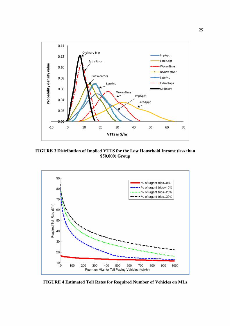
To further illustrate and compare the distributions of the implied VTTS corresponding to

all these situations we take a draw of 1000 sample points from the triangular distribution (the

distribution used for the travel time parameter) and estimate the VTTS values for the low income

group. Note that although the standard deviation of the distribution for the travel time parameter

is set to be equal to the mean, the heterogeneity in the means of travel time and toll parameters

results in different shapes to the distributions of VTTS corresponding to different situations.

Figure 3 shows that the VTTS for the LateApp situation t does not only have a large mean, but it

also has a large spread as compared to the ordinary and other urgent situations, indicating the

large variability of the VTTS for different travelers.

19

The preceding analysis clearly indicates a significant difference between a travelers’

typical VTTS on a ML and their VTTS in urgent situations. It is the VTTS based on typical

travel which generally serves as the basis to calculate travelers’ willingness to pay for a ML.

Therefore, engineers and planners are missing the added value that MLs have for travelers on

urgent trips. Based on previous studies and anecdotal evidence and information provided by ML

travelers we know that many individuals only use the MLs in urgent situations. This added value

is therefore unmeasured and the true value of MLs is underestimated. The following scenarios

illustrate this underestimation.

Assumptions:

• Total travelers in one direction on the freeway = 8000 veh/hr,

• Percent of travelers facing an urgent situation= 0, 10, 20 and 30. Of these

o 25 percent face urgent situation- ImpAppt,

o 25 percent face urgent situation- LateAppt,

o 12.5 percent face urgent situation- WorryTime,

o 12.5 percent face urgent situation-BadWeather,

o 12.5 percent face urgent situation- LateML,

o 12.5 percent face urgent situation- ExtraStops,

• Percent of ML travelers with low incomes (less than $50,000 )= 25 %,

• Percent of ML travelers with medium incomes ($50,000 to $100,000 )= 37%,

• Percent of ML travelers with low incomes (greater than $100,000) = 38%.

Using the above assumptions and the VTTS estimates we can evaluate the travel time

saving benefits offered by the managed lanes. We estimate these benefits for an increasing

20

number of toll paying vehicles, which is the number of vehicles that can fit on the managed lanes

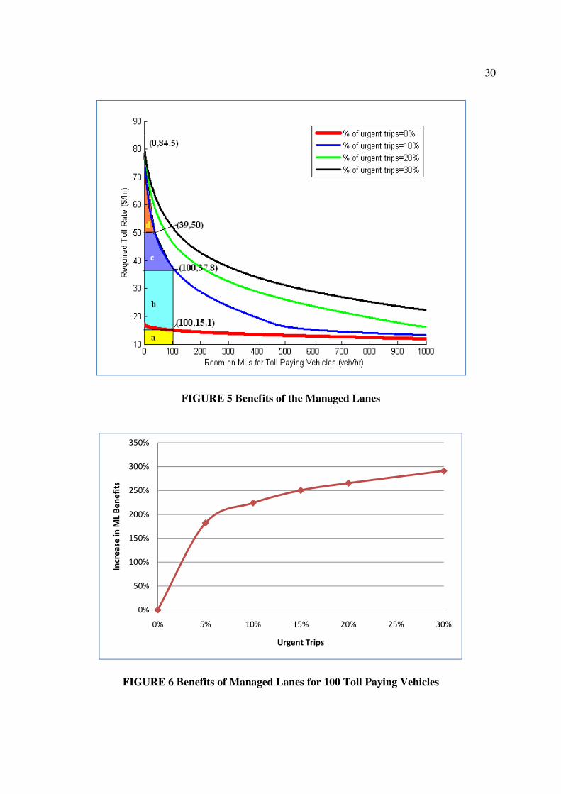
aside from toll-free HOVs (see Figure 4).

Figure 4 shows that by assuming all travelers are facing ordinary trips there is the

potential for significant underestimation of the value of travel time savings benefits obtained

from the managed lanes. For example, assume there is room for 100 more vehicles on the MLs

and that all 100 are on ordinary trips. This corresponds to results in hourly benefits identified by

the area a below the curve in Figure 5, which corresponds to the ordinary trip situations. This

area is approximately $1,635 (15.1*100+ (17.6-15.1)*100/2). However, if we assume just 10

percent of all 8,000 travelers are facing urgent, and not ordinary trips, the hourly benefits

increase to the area identified in Figure 5 by ‘a + b + c + d’ (c and d approximated as a triangle

for ease of calculation), which is approximated by $5,300.65 [(37.8*100 + (50-37.8)*39+(50-

37.8)*(100-39)/2+(84.5-50)*39/2)]. Hence, the average value of MLs without urgent trips is

approximately equal to $16.35 (1635/100) and the average value of MLs with 10-percent urgent

trips is equal to $53.01(5300.65/100). Though these are approximations, the indication is that if

managed lanes save 10 minutes of travel time, considering all 100 trips to be ordinary trips will

yield $272.5 (100*16.35*10/60) in traveler benefits. However, with 10 percent of all trips being

urgent trips, the benefits will be $883.4 (100*53.01*10/60). Hence, mistakenly classifying the 10

percent of urgent trips as ordinary trips would underestimate the approximate value of travel time

savings benefits by 224 percent (883.4-272.5/272.5*100) for those 100 travelers.

These approximations demonstrate that the assumed percentage of urgent trips affects the

value of these benefits; hence it calls for accurate estimation of the percentage of travelers facing

urgent trips and the percentage of urgent trips of each type using the traveler surveys. This is

shown by Figure 6 which plot the results for a case when there is additional room for 100 more

21

toll paying travelers on the MLs and when the there are approximately 10 minutes of travel time

savings offered by the MLs.

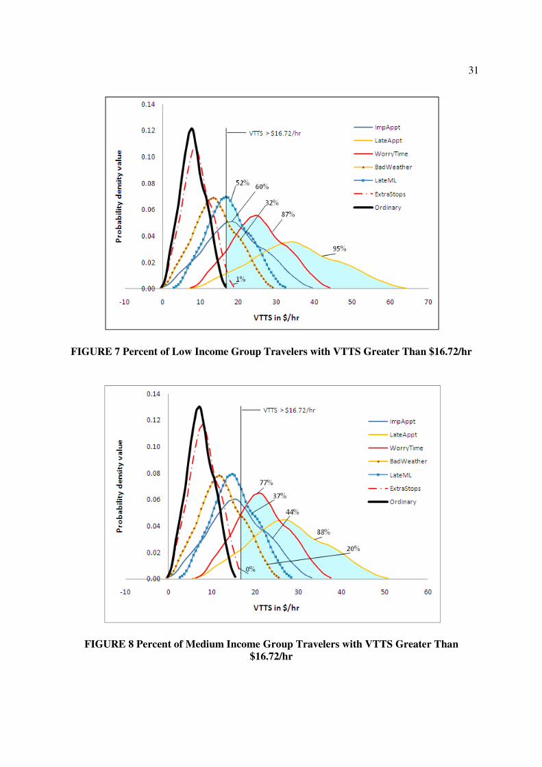
Note that the plots in Figure 4 are actually demand curves corresponding to each scenario

and these can also be used to set the toll rates on the MLs. When setting the toll rate for MLs it is

the travelers with the highest VTTS who are most likely to use the MLs and therefore the ones

by which the ML toll could be set. Using the model estimation results, it can be shown that the

high end of the high income group travelers in an ordinary situation will have VTTS equal to

$16.72/hr. Many low income travelers under different travel situations exceed this $16.72,

including:

• 60% facing the urgent situation-ImpAppt,

• 95% facing the urgent situation-LateAppt,

• 87% facing the urgent situation-WorryTime,

• 32% facing the urgent situation-BadWeather,

• 52% facing the urgent situation-LateML, and

• 1% facing the urgent situation-ExtraStops, (all represented by shaded area in

Figure 7).

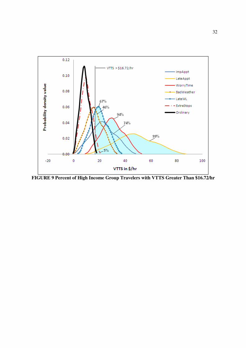
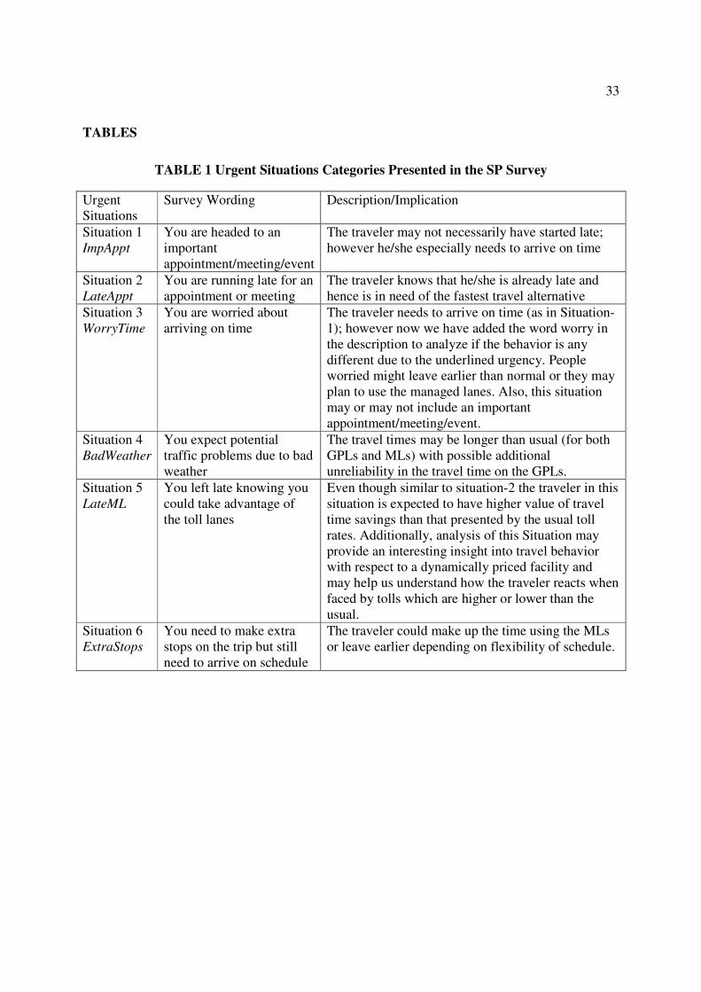
Similarly, many medium and high income travelers in urgent travel situations have VTTS greater

than the highest VTTS of the high income group travelers in an ordinary situation (that is

$16.72/hr) (see Figure 8 and Figure 9). Thus, many of the travelers from the medium and low

income groups who are on urgent trips will have VTTS greater than that of the travelers from the

high income group on ordinary trips. Hence, depending on the room for toll paying travelers on

the managed lanes, the entire group of toll paying travelers could be on urgent trips. Note that

22

these results depend on the assumed distribution of the VTTS used in this research. However,

similar results would be obtained using other reasonable assumptions regarding the distribution

of VTTS.

5. CONCLUSIONS

This research focused on estimates of the values of travel time savings (VTTS) for

ordinary situations as compared to six different urgent trip situations commonly faced by

travelers with an option of using managed lanes. An ordinary situation was defined as a typical

trip in the week prior to the survey. Urgent trip situations were represented by expected and

unexpected events potentially affecting an ordinary trip which is characterized by budget and

schedule constraints (such as business meetings and medical appointments). VTTS are estimated

using stated preference data collected via an internet survey of Katy Freeway travelers.

The findings indicate that travelers place a much higher value on their travel time when

faced by most of the urgent situations considered in this study. The mean of VTTS

corresponding to these urgent situations ranged from $8 to $47.5 per hour as compared to the

estimate of $7.4 to $8.6 per hour for the ordinary situations. Further, the study finds that the

implied means of VTTS for low and medium income group travelers facing most urgent

situations were higher than the high income traveler with the highest VTTS in an ordinary

situation (given our assumptions regarding the distribution of VTTS among travelers).

Due to this significant increase in the VTTS for travelers on urgent trips it is possible that

the majority of ML travelers are on urgent trips. This includes travelers from all income levels

as even low income travelers on urgent trips value their time more than many high income

23

travelers on regular trips. Thus travelers on MLs are likely to be from all income categories as

their need for (and value of) MLs varies mostly by trip urgency.

The second objective of the study was to better understand and estimate the value of

managed lanes. The results show that classifying urgent trips as ordinary trips can greatly

underestimate the total benefits of managed lanes to travelers. The example in section 4.2

assumes that only 10 percent of travelers take urgent trips and only 10 minutes of travel time

savings on a managed lane that could accommodate 100 toll paying vehicles. Under these

assumptions, the benefits of managed lanes for those 100 travelers would be more than three

times as much as predicted assuming only ordinary trips.

Therefore, using average VTTS for all travelers has the potential to greatly underestimate

the value of these MLs to travelers. This has significant policy implications since the benefits of

MLs (and of most transportation investments) are primarily derived from travel time savings.

Underestimating the value of ML travel time savings underestimates the benefits of MLs,

thereby reducing the likelihood of funding such facilities when investment decisions are based

on benefit-cost analysis. This study provides an important first step in the estimation of these

benefits using modified SP surveys and calls for identification of the proportion of travelers who

are taking a trip in an urgent situation such as the ones considered here.

The limitations of this study include a possible sampling bias (particularly with respect to

under-sampling low income travelers), possible measurement error in the income variable,

restrictive assumptions regarding the assumed distributions for the random parameters and

omitting the effects of variables other than travel time savings (such as travel time reliability or

penalty for late arrival) in the estimated VTTS. Incorporating these variables, and then

24

estimating the value of these other variables would be another way that engineers, economists

and planners may be able to estimate the true value of ML travel. Either method will require

continued research into the decision making process of travelers.

ACKNOWLEDGEMENTS

The authors recognize and appreciate that support for this research was provided by a grant from

the University Transportation Center for Mobility. Dr. Shaw also acknowledges support from a

U.S.D.A. Hatch grant. The authors wish to thank Dr. David Ungemah, an Associate Research

Scientist at Texas Transportation Institute at the time of this research and now with Parsons

Brinkerhoff, for all the support he provided in hosting the survey website. Additionally we would

like to thank HCTRA for helping with the collection of data for this study.

REFERENCES

Adamowicz, W., Louviere, J. and Williams, M., 1994. Combining stated and revealed preference methods for valuing environmental amenities. Journal of Environmental Economics and

Management 26, 271–292.

Austin Business Journal. 2009. American Internet Use Article June 3, http://austin.bizjournals.com/austin/stories/2009/06/01/daily32.html Accessed July 27, 2009.

Ben-Akiva, M., Bolduc, D., Walker, J., 2001. Specification, identification and estimation of the logit kernel (or continuous mixed logit) model, MIT Working paper, Department of Civil Engineering.

Bhat, C.R., 2001. Quasi-random maximum simulated likelihood estimation of the mixed multinomial logit model. Transportation Research Part B 35, 677-693.

Bhat C.R. and Castelar, S., 2002. A unified mixed logit framework for modeling revealed and stated preferences: formulation and application to congestion pricing analysis in the San Francisco Bay area, Transportation Research Part B 36 (7), 593–616.

Brownstone, D., Train, K., 1999. Forecasting new product penetration with flexible substitution patterns. Journal of Econometrics 89, 109–129.

25

Brownstone, D., Bunch, D. S., and Train, K.,2000. Joint mixed logit models of stated and revealed references for alternative-fuel vehicles. Transportation Research B, 34, 315-338.

Brownstone, D., Ghosh, A., Golob, T.F. and Van Amelsfort, D., 2003. Drivers willingness-to-pay to reduce travel time: evidence from the San Diego I-15 congestion pricing project. Transportation Research A 37, 373-387.

Brownstone, D. and Small, K.A, 2005. Valuing time and reliability: assessing the evidence from road pricing demonstrations, Transportation Research A, 39(4), 279-293.

Burris, M.W. and Stockton, W.R. 2004. HOT lanes in Houston – Six years of experience, Journal of Public Transportation 7(4), 1-21.

Burris, M.W. and Figueroa, C.F. 2006. Analysis of traveler characteristics by mode choice in HOT corridors, Journal of the Transportation Research Forum. 45(2), 103 – 117.

Burris, M. and Patil, S. 2009. Estimating Benefits of Managed Lanes. University Transportation Center for Mobility, Texas Transportation Institute, College Station, Texas.

Census, 2007, State and County QuickFacts, U.S. Census Bureau, http://quickfacts.census.gov/qfd/index.html. Accessed May 15, 2009.

Collier, T. and Goodin, G.D., 2002. Managed lanes: More efficient use of the freeway system. TTI Research Report 4160-5-p1, College Station, Texas.

Dosman, D. and Adamowicz, W., 2006. Combining stated and revealed preference data to construct an empirical examination of intrahousehold bargaining, Review of the Economics of

the Household 4, 15-34.

Ghosh, A., 2001. Valuing time and reliability: commuters’ mode choice from a real time congestion pricing experiment. Ph.D. Dissertation, Department of Economics, University of California at Irvine.

Greene, W.H., Hensher, D.A., Rose, J., 2006. Accounting for heterogeneity in the variance of unobserved effects in mixed logit models. Transportation Research B 4 (1), 75–92.

Greene, W., 2007. NLOGIT Version 4.0: Reference Guide, Plainview, NY, Economertric Software.

Greene, W.H. and Hensher, D.A., 2007. Heteroscedastic control for random coefficients and error components in mixed logit, Transportation Research E 43, 610–623.

HCTRA 2009, Harris County Toll Road Authority, Toll Road Information – Overview https://www.hctra.org/tollroads/. Accessed May 15, 2009.

Hensher, D.A., Rose, J., Greene, W.H., 2005. Applied choice analysis: A primer. Cambridge University Press, Cambridge.

Hensher, D.A., Rose, M.J., Greene, W.H., 2008. Combining RP and SP data: Biases in using the nested logit ‘trick’-contrasts with flexible mixed logit incorporating panel and scale effects, Journal of Transport Geography 16, 126-133.

26

Patil, S., Burris, M., Shaw, D., 2011. Travel using managed lanes: An application of a stated choice model for Houston, Texas, In Press, Transport Policy.

Revelt, D., Train, K., 1998. Mixed logit with repeated choices: Households’ choices of appliance efficiency level. Review of Economics and Statistics 80, 1–11.

Small, K.A., Noland, R., Chu, X., Lewis, D., 1999. Valuation of travel-time savings and predictability in congested conditions for highway user-cost estimation, National Cooperative Highway Research, Report 431, Transportation Research Board, National Research Council, Washington, D.C., 1999.

Sullivan, E., Blakely, K., Daly, J., Gilpin, J., Mastako, K., Small, K., Yan, J., 2000. Continuation study to evaluate the impacts of the SR91 value-priced express lanes: final report. California Polytechnic State University at San Luis Obispo, December http://ceenve.ceng.calpoly.edu/sullivan/SR91.

Tilahun, N. and Levinson, D., 2008. Willingness to pay and the cost of delay on I-394 high occupancy/toll lanes. Presented at the 87th Annual Meeting of the Transportation Research

Board, Washington, D.C.

Train, K., 1998. Recreation demand models with taste differences over people. Land Economics 74, 230–239.

Train, K., 2003. Discrete Choice Methods with Simulation. Cambridge University Press, Cambridge.

Tseng Y.Y and Verhoef, E., 2008. Value of time by time of day: A stated-preference study, Transportation Research Part B 42 (7), 607-618.

TxDOT 2009, Katy Freeway Website, Texas Department of Transportation, www.katyfreeway.org/. Accessed May 15, 2009.

27

FIGURES

FIGURE 1 Freeway Network in and Around City of Houston, Texas

28

FIGURE 2 Typical Stated Preference Question in the Survey

29

ImpAppt

LateAppt

WorryTime

BadWeather

LateML

ExtraStops

Ordinary Trip

0.00

0.02

0.04

0.06

0.08

0.10

0.12

0.14

-10 0 10 20 30 40 50 60 70

Pro

ba

bil

ity

de

nsi

ty v

alu

e

VTTS in $/hr

ImpAppt

LateAppt

WorryTime

BadWeather

LateML

ExtraStops

Ordinary

FIGURE 3 Distribution of Implied VTTS for the Low Household Income (less than $50,000) Group

FIGURE 4 Estimated Toll Rates for Required Number of Vehicles on MLs

0 100 200 300 400 500 600 700 800 900 100010

20

30

40

50

60

70

80

90

Required T

oll

Rate

($/h

r)

Room on MLs for Toll Paying Vehicles (veh/hr)

% of urgent trips=0%

% of urgent trips=10%

% of urgent trips=20%

% of urgent trips=30%

30

FIGURE 5 Benefits of the Managed Lanes

FIGURE 6 Benefits of Managed Lanes for 100 Toll Paying Vehicles

0%

50%

100%

150%

200%

250%

300%

350%

0% 5% 10% 15% 20% 25% 30%

Incr

ea

se in

ML

Be

ne

fits

Urgent Trips

31

FIGURE 7 Percent of Low Income Group Travelers with VTTS Greater Than $16.72/hr

FIGURE 8 Percent of Medium Income Group Travelers with VTTS Greater Than $16.72/hr

32

FIGURE 9 Percent of High Income Group Travelers with VTTS Greater Than $16.72/hr

33

TABLES

TABLE 1 Urgent Situations Categories Presented in the SP Survey

Urgent Situations

Survey Wording Description/Implication

Situation 1 ImpAppt

You are headed to an important appointment/meeting/event

The traveler may not necessarily have started late; however he/she especially needs to arrive on time

Situation 2 LateAppt

You are running late for an appointment or meeting

The traveler knows that he/she is already late and hence is in need of the fastest travel alternative

Situation 3 WorryTime

You are worried about arriving on time

The traveler needs to arrive on time (as in Situation-1); however now we have added the word worry in the description to analyze if the behavior is any different due to the underlined urgency. People worried might leave earlier than normal or they may plan to use the managed lanes. Also, this situation may or may not include an important appointment/meeting/event.

Situation 4 BadWeather

You expect potential traffic problems due to bad weather

The travel times may be longer than usual (for both GPLs and MLs) with possible additional unreliability in the travel time on the GPLs.

Situation 5 LateML

You left late knowing you could take advantage of the toll lanes

Even though similar to situation-2 the traveler in this situation is expected to have higher value of travel time savings than that presented by the usual toll rates. Additionally, analysis of this Situation may provide an interesting insight into travel behavior with respect to a dynamically priced facility and may help us understand how the traveler reacts when faced by tolls which are higher or lower than the usual.

Situation 6 ExtraStops

You need to make extra stops on the trip but still need to arrive on schedule

The traveler could make up the time using the MLs or leave earlier depending on flexibility of schedule.

34

TABLE 2 Model Estimation Results for MNL and Mixed Logit Models

Attribute Alternative(s) MNL Model Mixed Logit model

Coeff. t-ratio Coeff. t-ratio

ASC:CP-GPL CP-GPL -0.66 -10.53 R:-2.22 -11.49

ASC:DA-ML DA-ML -1.04 -8.20 R:-2.44 -7.66

ASC:HOV2-ML HOV2-ML -0.58 -4.45 R:-1.82 -8.74

ASC:HOV3+-ML HOV3+-ML -1.95 -14.23 R:-4.64 -21.82

Travel Time (minutes) All -0.11 -24.16 R:-0.24 -31.41

Toll ($) All -0.90 -19.17 -1.81 -42.02

Drove alone for last trip (dv) CP-GPL -2.99 -28.77 -5.59 -23.28

Trip purpose commute/work (dv) CP-GPL 0.14 1.87

Male (dv) (male =1, female=0) CP-GPL -0.17 -2.40

Age between 25 and 54 (dv) CP-GPL 0.53 2.49

Drove alone for last trip (dv) DA-ML -0.27 -5.04

Trip Length (miles) DA-ML 0.01 4.14 0.04 5.12 Toll tag subscriber (dv) (1= owns a toll tag) DA-ML 0.57 5.13 1.12 3.75

Drove alone for last trip (dv) HOV2-ML -2.41 -30.42 -4.07 -25.33

Trip purpose commute/work (dv) HOV2-ML 0.22 3.23

Trip Length (miles) HOV2-ML 0.02 4.77 0.04 3.81

Age between 25 and 54 (dv) HOV2-ML -0.28 -3.80

Number of people in household HOV2-ML 0.08 2.80

Male (dv) (male =1, female=0) HOV2-ML -0.49 -7.56 -0.82 -5.68

Single Adult Household (dv) HOV2-ML -0.36 -3.40 -0.47 -2.29

Number of vehicles in the household HOV2-ML -0.08 -2.39

Drove alone for last trip (dv) HOV3+-ML -2.88 -25.36 -5.26 -20.14

Trip Length (miles) HOV3+-ML 0.01 2.49

Male (dv) (male =1, female=0) HOV3+-ML -0.22 -2.49

Age between 25 and 54 (dv) HOV3+-ML 0.32 3.08

Standard deviation of Random Parameters(:)

ASC:CP-GPL CP-GPL 3.35 30.08

ASC:DA-ML DA-ML 1.92 25.74

ASC:HOV2-ML HOV2-ML 2.37 24.54

ASC:HOV3+-ML HOV3+-ML 3.61 20.71

Travel Time (minutes) All 0.24 31.41

Urgent to ordinary situations Scale parameter All 0.64 6.68

35

TABLE 2- Continued

Attribute Alternative(s) MNL Model Mixed Logit

Model

Coeff. t-ratio Coeff. t-ratio

Interactions in MNL /Heterogeneity (P) in mean in mixed logit

Travel Time* ImpAppt All 0.00 -0.40 0

Travel Time* LateAppt All -0.02 -1.72 -0.07 -4.32

Travel Time* WorryTime All -0.07 -5.22 -0.11 -5.18

Travel Time* BadWeather All -0.03 -2.19 0

Travel Time* LateML All -0.02 -2.04 -0.06 -2.91

Travel Time* ExtraStops All 0.00 -0.39 0

Toll ($)* ImpAppt All 0.54 10.14 1.05 15.21

Toll ($)* LateAppt All 0.72 15.29 1.28 17.01

Toll ($)* WorryTime All 0.47 9.10 0.98 11.60 Toll ($)* BadWeather All 0.36 6.32 0.78 10.42

Toll ($)* LateML All 0.44 8.06 0.77 8.63

Toll ($)* ExtraStops All 0.13 1.98 0.21 2.90 Toll ($)* Medium Household Income ($50,000- 100,000) (dv) All 0.01 0.33 -0.14 -5.50 Toll ($)*High Household Income(>$100,000) (dv) All 0.16 3.87 0.14 5.49

Error Components for alternatives and nests of alternatives parameters (θ)

Standard deviation , θQ GPL alts. 0.27 3.42

Standard deviation , θD ML alts. 2.10 7.27

Heterogeneity around standard deviation of error components effect ()

Male (dv) (male=1, female=0) GPL alts 1.63 6.03

Number of vehicles in the household GPL alts 0.16 3.93

Male (dv) (male=1, female=0) ML alts -1.06 -5.99

Number of vehicles in the household ML alts -0.06 -1.10

Log-likelihood at convergence -13467.43 -10722.10

Adjusted ρc2 0.28 0.42

Notes dv=dummy variable, R: Mean of the random parameter estimates, Adjusted ρc2 =1-.r3|*|O

where,

bb.73 log-likelihood for the estimated model, K= number of parameters in the estimated model,

bb* log-likelihood for the constants only model, Kc= number of parameters in the constants only

model, = Represents spread of the distribution (std. dev.= spread/√6), ASC= Alternative Specific

Coefficient

36

TABLE 3 Implied Mean VTTS for Ordinary and Urgent Situations

Situation

Mean VTTS ($/hr) for Categories of

Household Income ($/year)

Low-

< 50,000

Medium

50,000 -100,000

High-

>100,000

Ordinary 7.9 7.4 8.6

Headed to an important

appointment/meeting/event (ImpAppt) 18.7 15.9 22.8

Running late for an appointment or meeting

(LateAppt) 35.2 27.9 47.5

Worried about arriving on time (WorryTime) 25.0 21.5 30.0

Expecting potential traffic problems due to bad

weather (BadWeather) 13.9 12.2 16.0

Left late knowing you could take advantage of

the toll lanes (LateML) 17.0 15.0 19.6

Need to make extra stops on the trip but still

need to arrive on schedule (ExtraStops) 9.0 8.3 9.8