Embed Size (px)
Citation preview
Variant Calling (using High-‐throughput Sequencing Data)
Bioinforma�cs for Molecular Biology 2014
Tim Hughes
Downloading data
Wiki pages for zip file
Backup is usb s�ck
INTRODUCTION
What is variant calling and why do it?
What is varia�on? – Varia�on through muta�on – What kind of varia�on occurs? SNPs, indels, structural varia�on
Variant calling – Acquire data on sequence – Make an inference on whether a variant is present rela�ve to a reference
sequence
Why perform variant calling? – Congenital disease – Case control studies
Different types of variant calling – probe assays – microarrays – sequencing (low and high through-‐put)
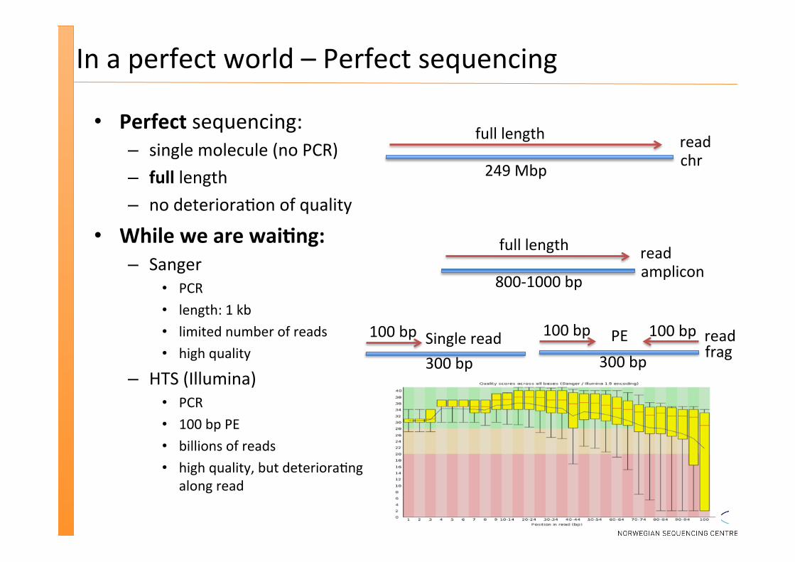
In a perfect world – Perfect sequencing
Perfect sequencing: – single molecule (no PCR) – full length – no deteriora�on of quality
While we are wai�ng: – Sanger
PCR length: 1 kb limited number of reads high quality
– HTS (Illumina) PCR 100 bp PE billions of reads high quality, but deteriora�ng
along read
100 bp 100 bp
300 bp frag read
full length
249 Mbp chr read
full length
800-‐1000 bp amplicon read
100 bp
300 bp Single read PE
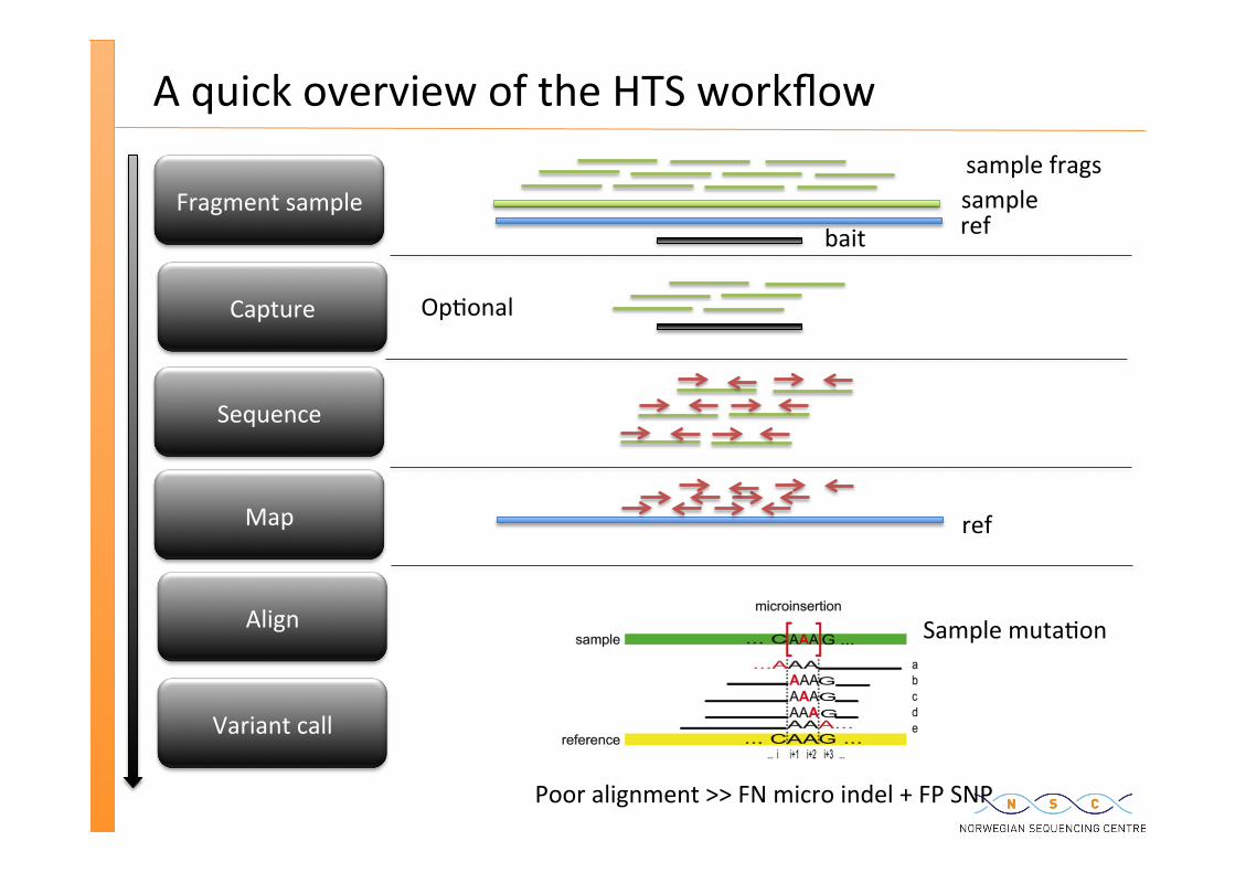
A quick overview of the HTS workflow
Fragment sample
Capture
Sequence
Map
Align
Variant call
ref
sample frags sample
bait
ref
Sample muta�on
Poor alignment >> FN micro indel + FP SNP
Op�onal
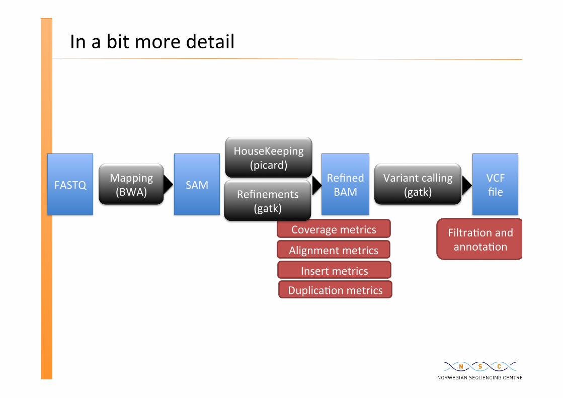
In a bit more detail
FASTQ Mapping (BWA) SAM
HouseKeeping (picard)
Variant calling (gatk)
Refined BAM
VCF file
Coverage metrics Filtra�on and annota�on Alignment metrics
Insert metrics
Duplica�on metrics
Refinements (gatk)
GSA team at the Broad Ins�tute
A large frac�on of the materials and so�ware in this course are produced by the Genome Sequencing and Analysis Group team at the Broad Ins�tute
Informa�on sources – h�p://www.broadins�tute.org/gsa/wiki – h�p://www.getsa�sfac�on.com/gsa
People – Mark A. DePristo, Manager of Medical and Popula�on Gene�cs Analysis – Eric Banks, Team Lead – Guillermo del Angel – Ryan Poplin – Kiran Garimella, Team Lead – Mauricio Carneiro – Chris Hartl – Khalid Shakir, Team Lead – Ma�hew Hanna – David Roazen
Others at the Broad – Heng Li: samtools and bwa – Tim Fennell: picard – Alec Wysoker: picard
And others outside the Broad – sources at bo�om of slides
Overview of topics (not in chrono order)
So�ware and datasets Fastq format Read mapping (SAM/BAM format) IGV Variant calling (VCF format) Metrics reports (esp coverage – BED format) Alignment refinement Base quality score recalibra�on Variant annota�on and filtra�on
Because of circumstances (shortened course) – exercises will NOT involve computa�on – we will work with pre-‐computed results found at the central URL
DATASETS
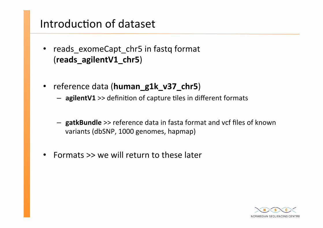
Introduc�on of dataset
reads_exomeCapt_chr5 in fastq format (reads_agilentV1_chr5)
reference data (human_g1k_v37_chr5) – agilentV1 >> defini�on of capture �les in different formats
– gatkBundle >> reference data in fasta format and vcf files of known variants (dbSNP, 1000 genomes, hapmap)
Formats >> we will return to these later
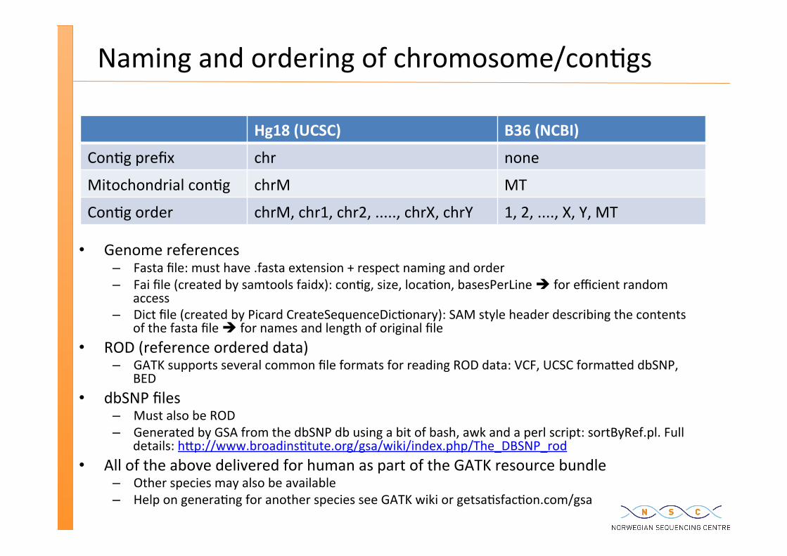
Naming and ordering of chromosome/con�gs
Hg18 (UCSC) B36 (NCBI)
Con�g prefix chr none
Mitochondrial con�g chrM MT
Con�g order chrM, chr1, chr2, ....., chrX, chrY 1, 2, ...., X, Y, MT
Genome references – Fasta file: must have .fasta extension + respect naming and order – Fai file (created by samtools faidx): con�g, size, loca�on, basesPerLine è for efficient random
access – Dict file (created by Picard CreateSequenceDic�onary): SAM style header describing the contents
of the fasta file è for names and length of original file ROD (reference ordered data)
– GATK supports several common file formats for reading ROD data: VCF, UCSC forma�ed dbSNP, BED
dbSNP files – Must also be ROD – Generated by GSA from the dbSNP db using a bit of bash, awk and a perl script: sortByRef.pl. Full
details: h�p://www.broadins�tute.org/gsa/wiki/index.php/The_DBSNP_rod All of the above delivered for human as part of the GATK resource bundle
– Other species may also be available – Help on genera�ng for another species see GATK wiki or getsa�sfac�on.com/gsa
GENETICS 101
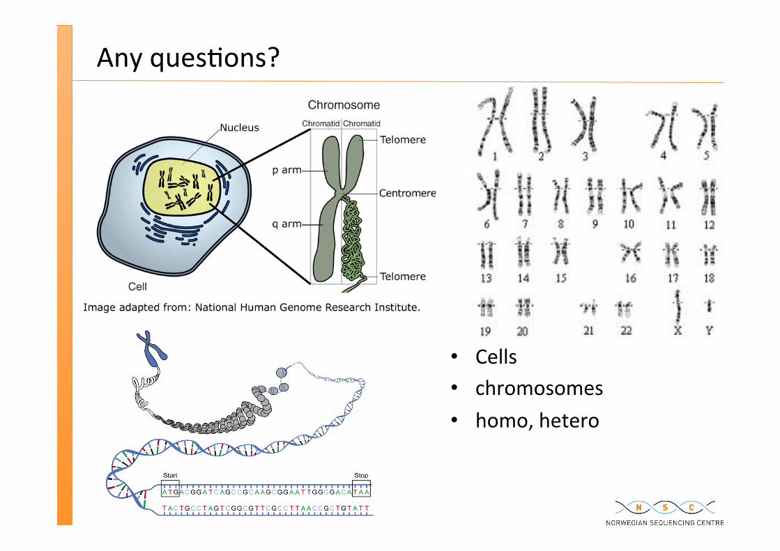
Any ques�ons?
Cells chromosomes homo, hetero
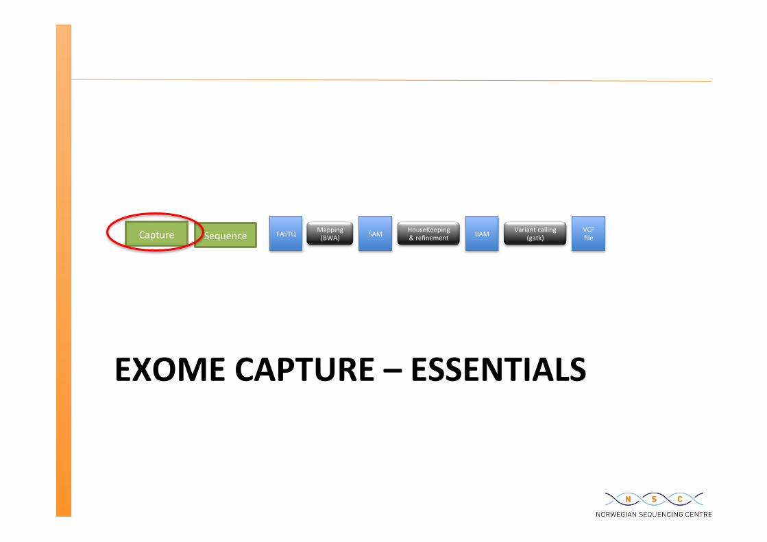
EXOME CAPTURE – ESSENTIALS
FASTQ Mapping (BWA) SAM HouseKeeping
& refinement Variant calling
(gatk) BAM VCF file Capture Sequence
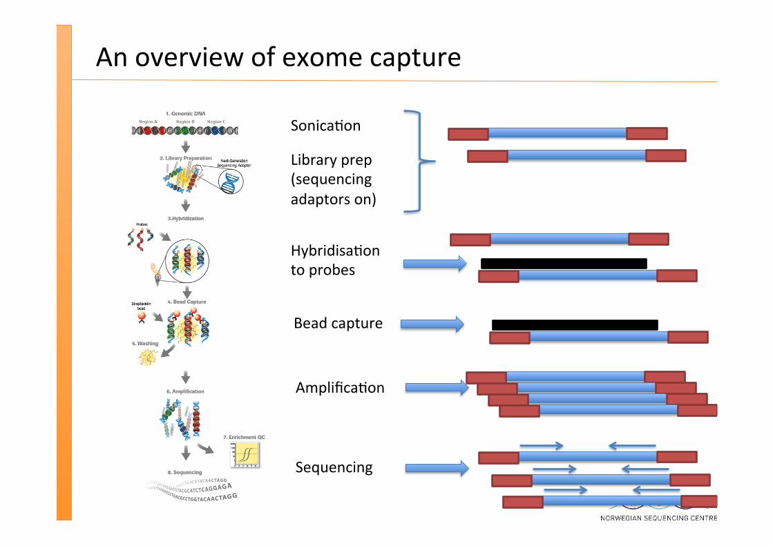
An overview of exome capture
Sonica�on
Library prep (sequencing adaptors on)
Hybridisa�on to probes
Bead capture
Amplifica�on
Sequencing
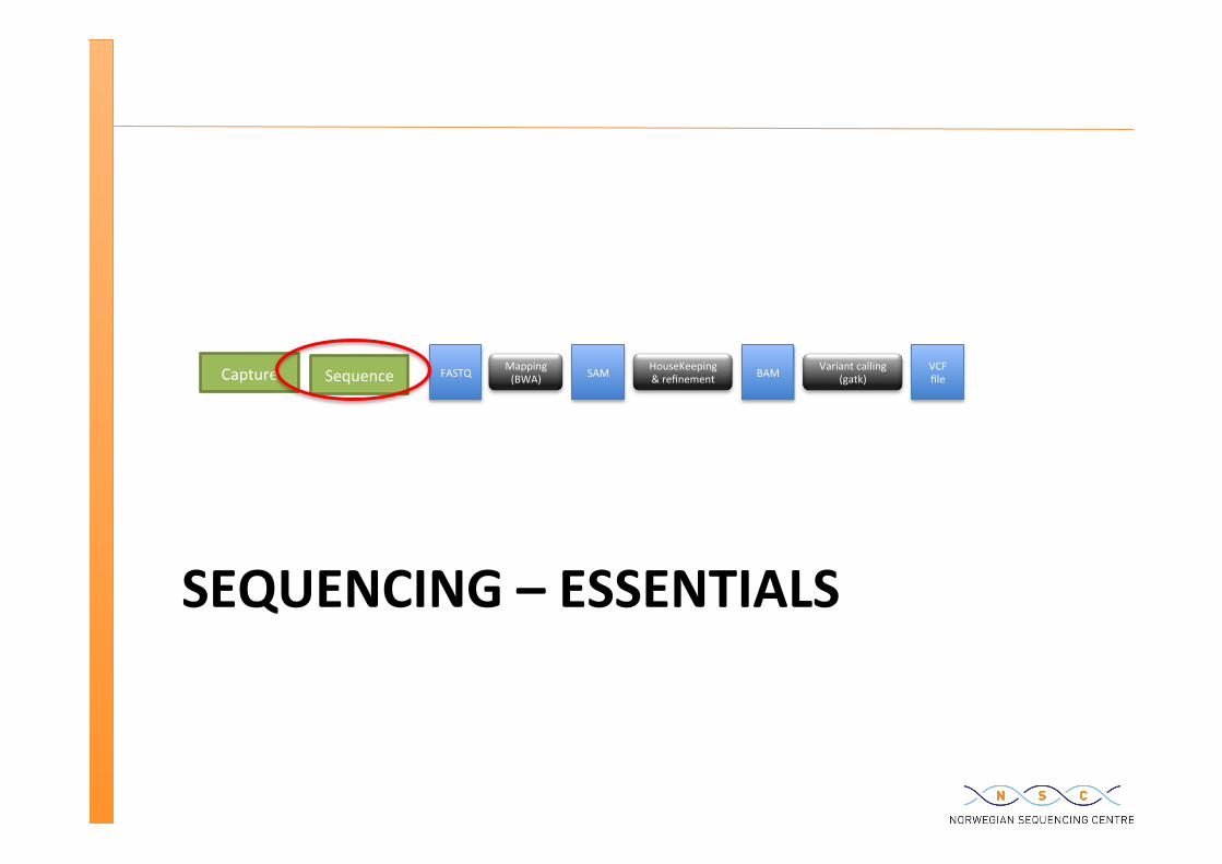
SEQUENCING – ESSENTIALS
FASTQ Mapping (BWA) SAM HouseKeeping
& refinement Variant calling
(gatk) BAM VCF file Capture Sequence
Sequencing
Covered by Robert
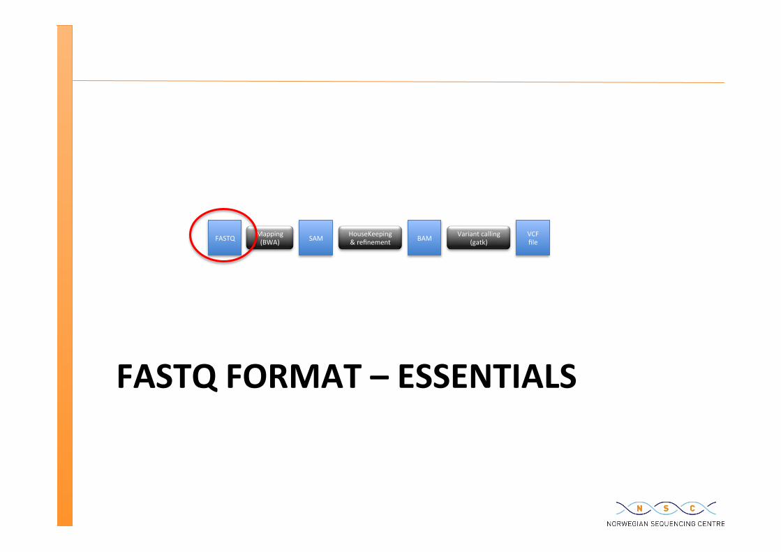
FASTQ FORMAT – ESSENTIALS
FASTQ Mapping (BWA) SAM HouseKeeping
& refinement Variant calling
(gatk) BAM VCF file
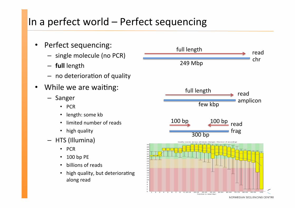
In a perfect world – Perfect sequencing
Perfect sequencing: – single molecule (no PCR) – full length – no deteriora�on of quality
While we are wai�ng: – Sanger
PCR length: some kb limited number of reads high quality
– HTS (Illumina) PCR 100 bp PE billions of reads high quality, but deteriora�ng
along read
100 bp 100 bp
300 bp frag read
full length
249 Mbp chr read
full length
few kbp amplicon read
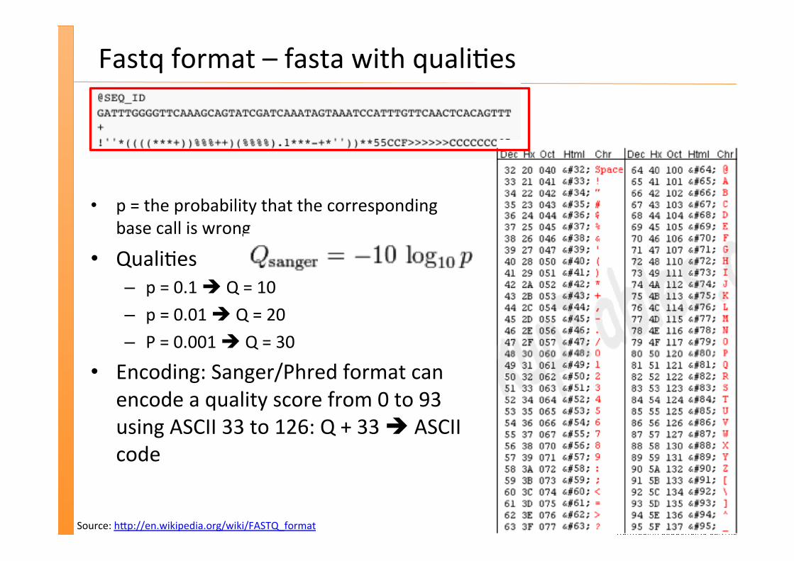
Fastq format – fasta with quali�es
p = the probability that the corresponding base call is wrong
Quali�es – p = 0.1 è Q = 10 – p = 0.01 è Q = 20 – P = 0.001 è Q = 30
Encoding: Sanger/Phred format can encode a quality score from 0 to 93 using ASCII 33 to 126: Q + 33 è ASCII code
Source: h�p://en.wikipedia.org/wiki/FASTQ_format
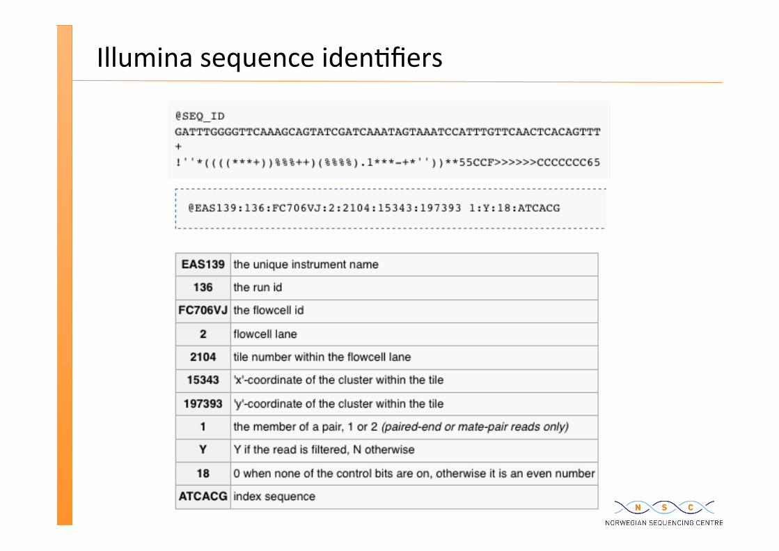
Illumina sequence iden�fiers
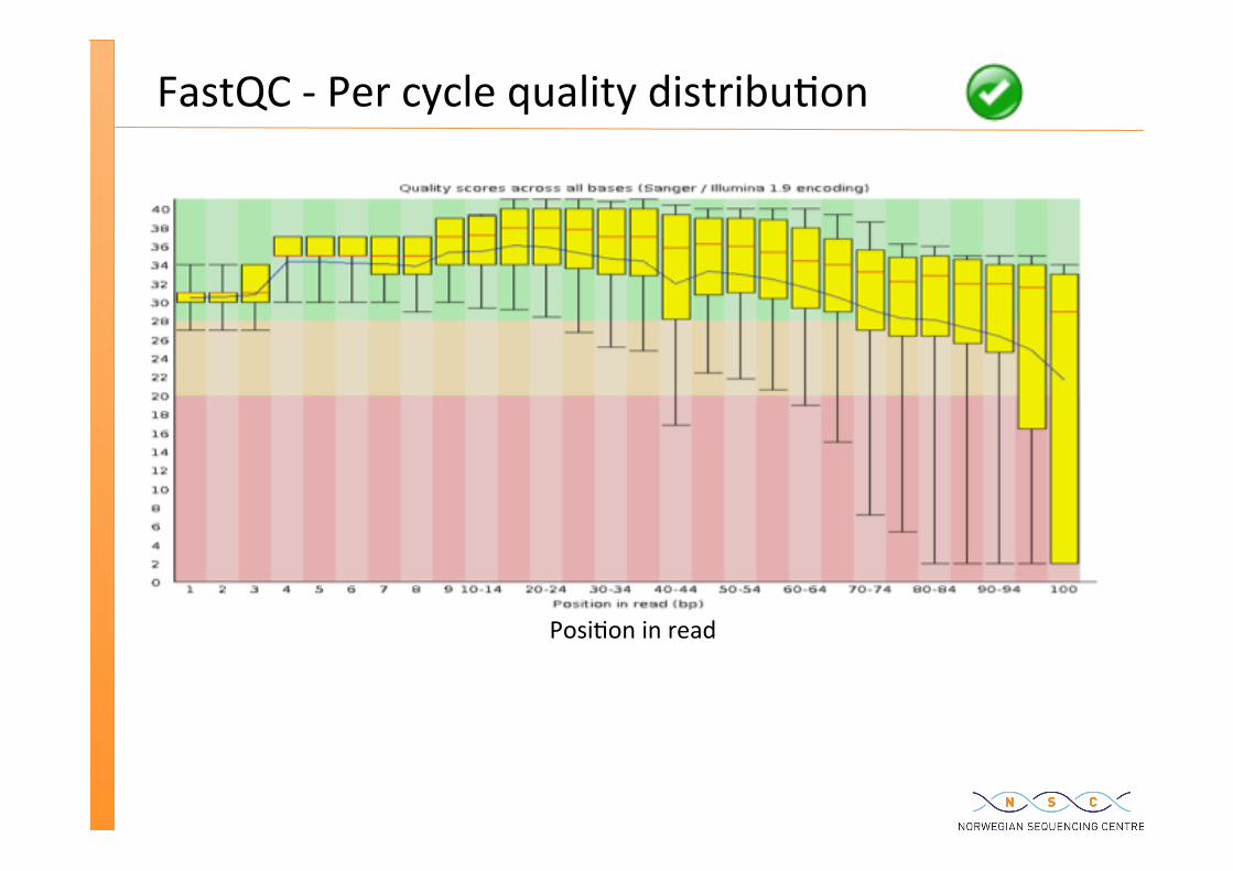
FastQC -‐ Per cycle quality distribu�on
Posi�on in read
%
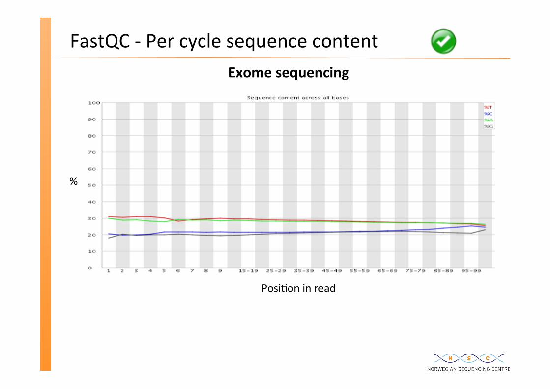
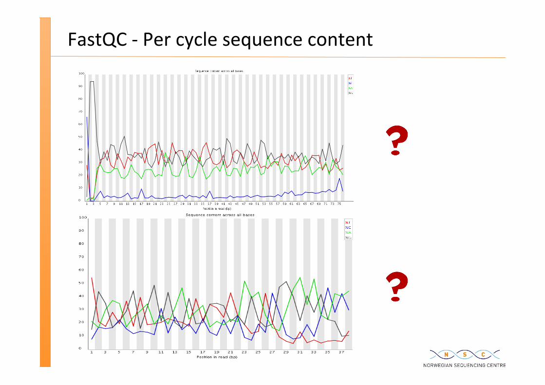
FastQC -‐ Per cycle sequence content
Posi�on in read
%
Exome sequencing
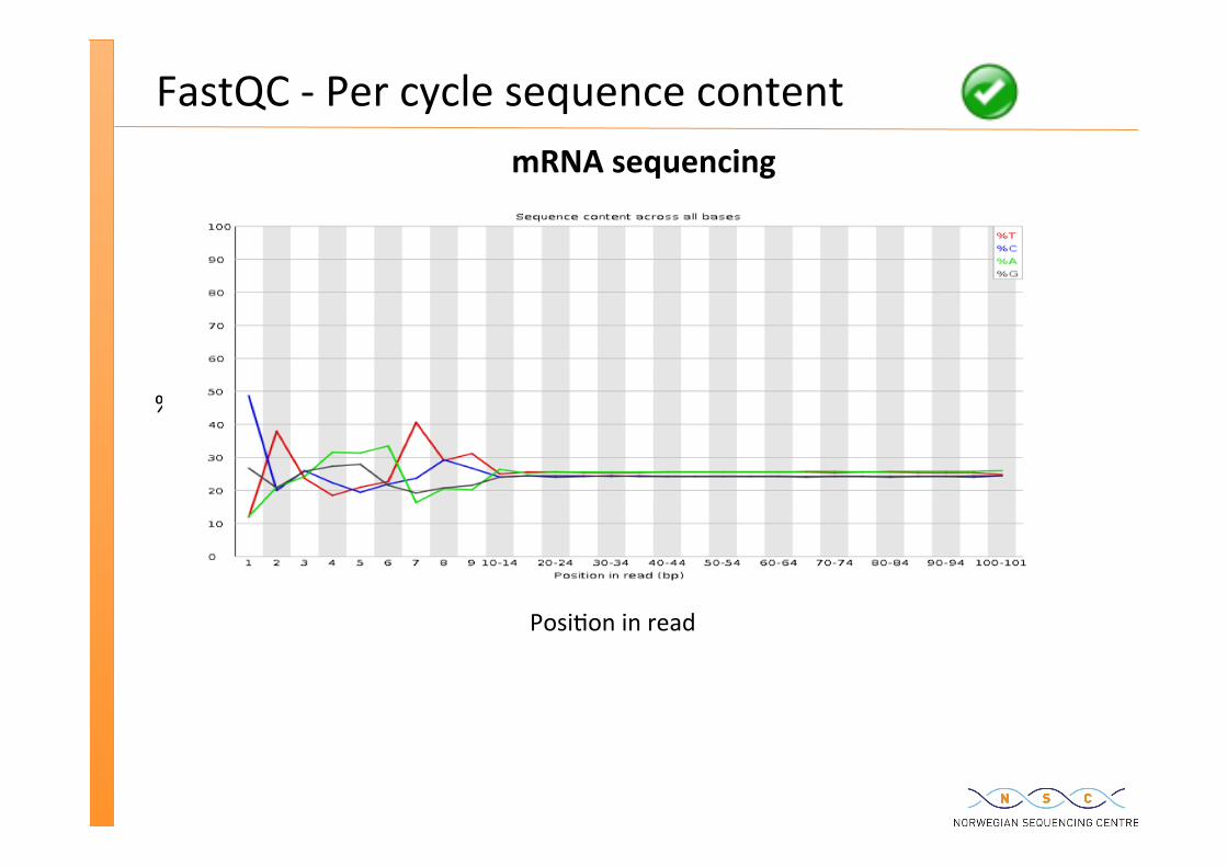
FastQC -‐ Per cycle sequence content
Posi�on in read
%
mRNA sequencing
FastQC -‐ Per cycle sequence content
Manipula�ng fasta and fastq files
Fastx toolkit: h�p://hannonlab.cshl.edu/fastx_toolkit/
FASTQ trimmer
FASTQ quality filter
FASTQ quality trimmer
Can do most of the obvious manipula�ons of fastq/a you may need
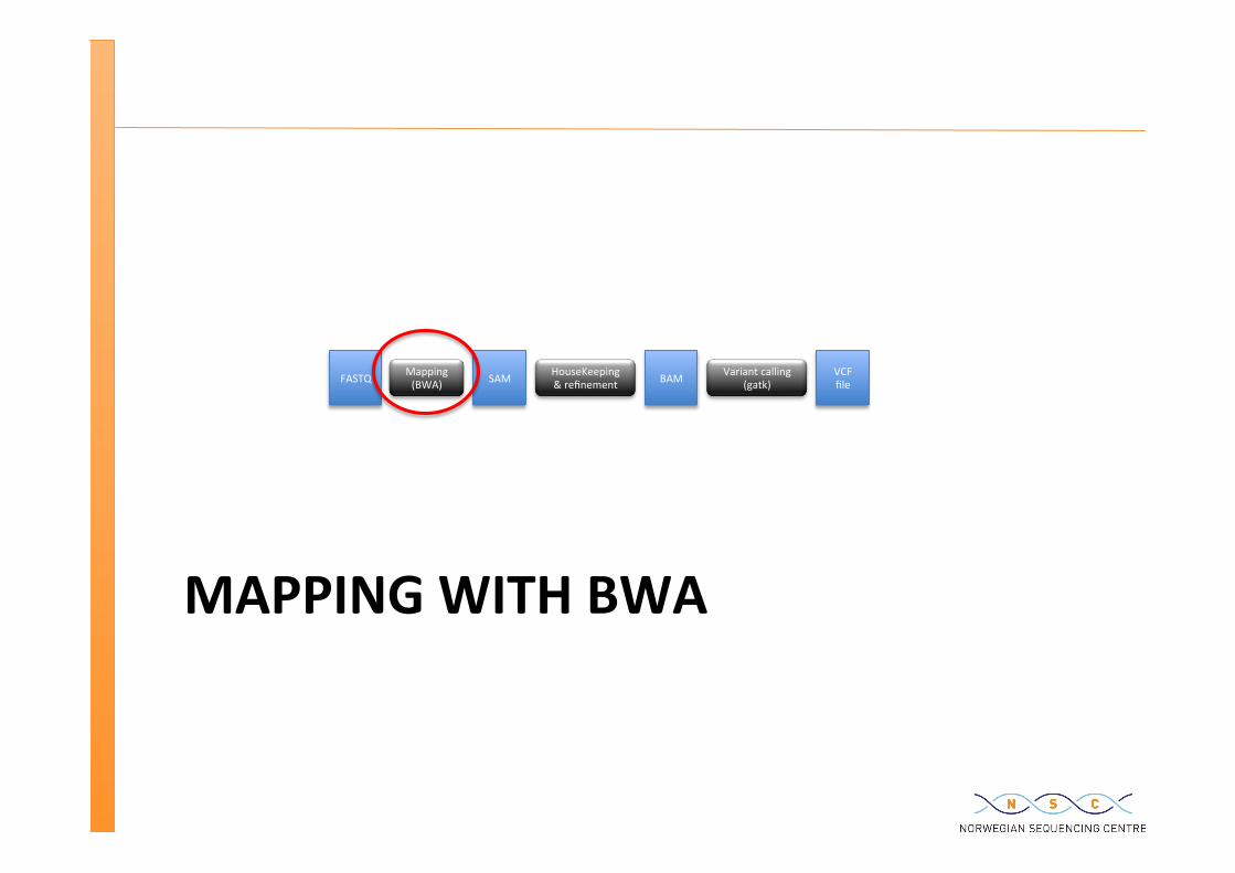
FASTQ Mapping (BWA) SAM HouseKeeping
& refinement Variant calling
(gatk) BAM VCF file
MAPPING WITH BWA
Why mapping?
The biggest difference with Sanger – we did NOT design and use primers for sequence amplifica�on – we sonicated – >> we do not know where the reads “originate” from
For each read – we need to determine its likely origin – how likely it is that we have correctly iden�fied its origin
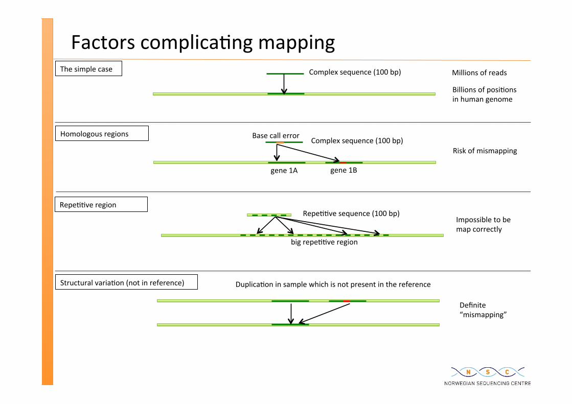
Factors complica�ng mapping Millions of reads
Billions of posi�ons in human genome
Complex sequence (100 bp) The simple case
Homologous regions Complex sequence (100 bp)
gene 1A gene 1B
Base call error
Repe��ve region Repe��ve sequence (100 bp)
big repe��ve region
Structural varia�on (not in reference) Duplica�on in sample which is not present in the reference
Risk of mismapping
Impossible to be map correctly
Definite “mismapping”
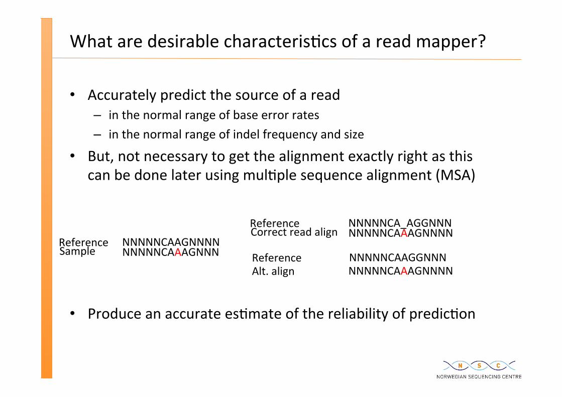
What are desirable characteris�cs of a read mapper?
Accurately predict the source of a read – in the normal range of base error rates – in the normal range of indel frequency and size
But, not necessary to get the alignment exactly right as this can be done later using mul�ple sequence alignment (MSA)
Produce an accurate es�mate of the reliability of predic�on
NNNNNCAAGNNNN NNNNNCAAAGNNN
Reference Sample
NNNNNCA_AGGNNN NNNNNCAAAGNNNN
Reference Correct read align
Alt. align NNNNNCAAAGNNNN NNNNNCAAGGNNN Reference
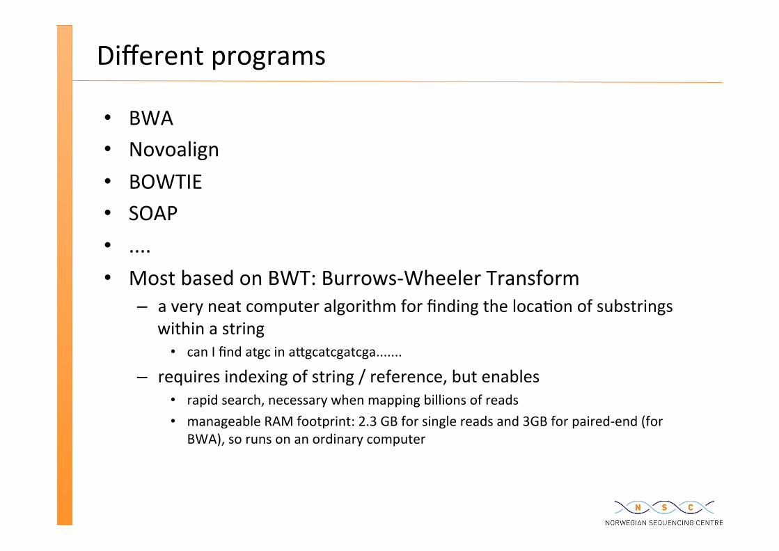
Different programs
BWA Novoalign BOWTIE SOAP .... Most based on BWT: Burrows-‐Wheeler Transform – a very neat computer algorithm for finding the loca�on of substrings
within a string can I find atgc in a�gcatcgatcga.......
– requires indexing of string / reference, but enables rapid search, necessary when mapping billions of reads manageable RAM footprint: 2.3 GB for single reads and 3GB for paired-‐end (for
BWA), so runs on an ordinary computer
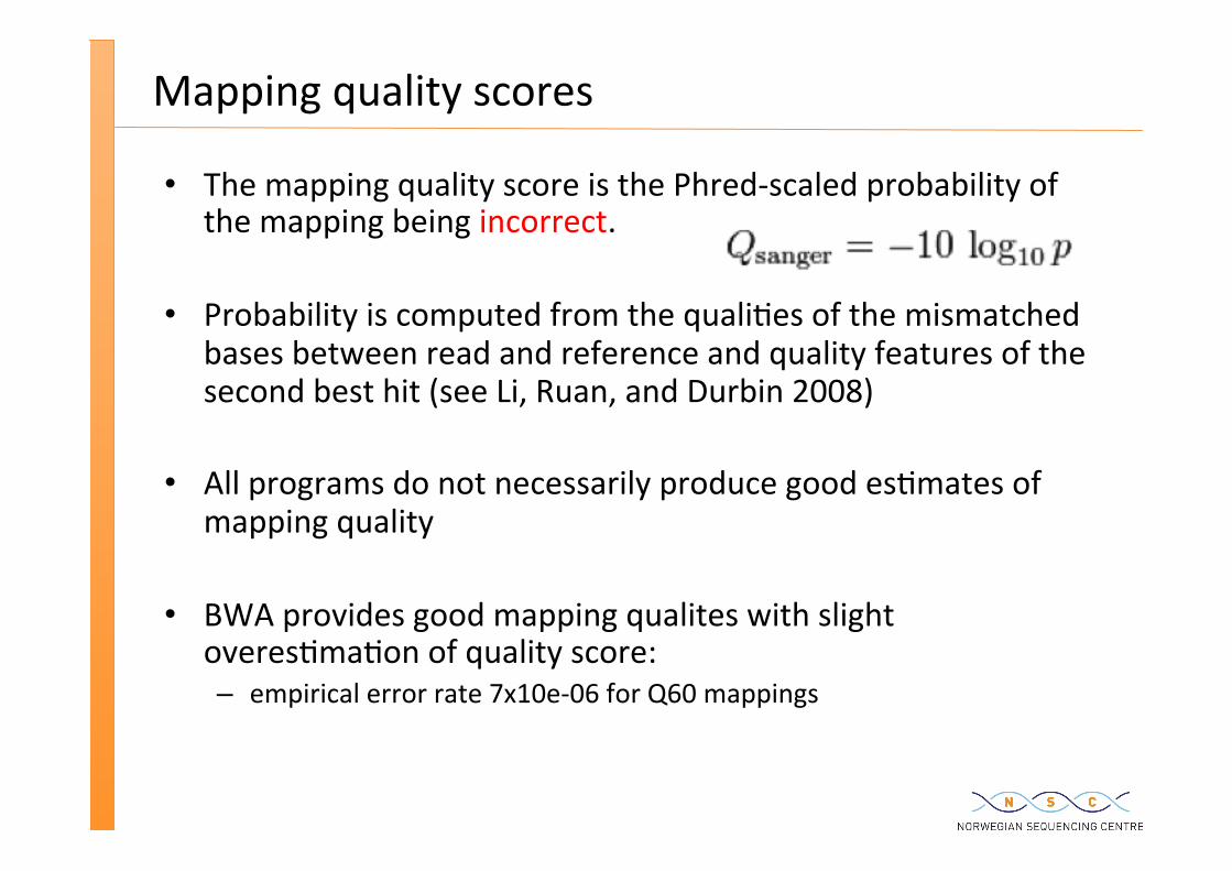
Mapping quality scores
The mapping quality score is the Phred-‐scaled probability of the mapping being incorrect.
Probability is computed from the quali�es of the mismatched bases between read and reference and quality features of the second best hit (see Li, Ruan, and Durbin 2008)
All programs do not necessarily produce good es�mates of mapping quality
BWA provides good mapping qualites with slight overes�ma�on of quality score: – empirical error rate 7x10e-‐06 for Q60 mappings
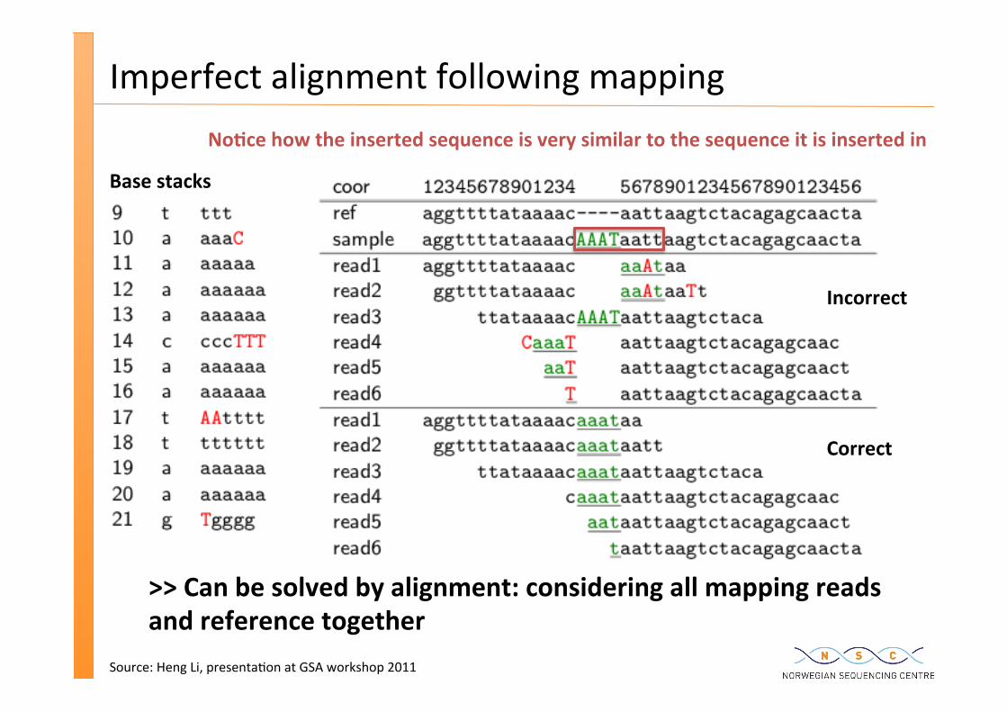
Imperfect alignment following mapping
Source: Heng Li, presenta�on at GSA workshop 2011
Incorrect
Correct
Base stacks
>> Can be solved by alignment: considering all mapping reads and reference together
No�ce how the inserted sequence is very similar to the sequence it is inserted in
FASTQ Mapping (BWA) SAM HouseKeeping
& refinement Variant calling
(gatk) BAM VCF file
SAM FORMAT
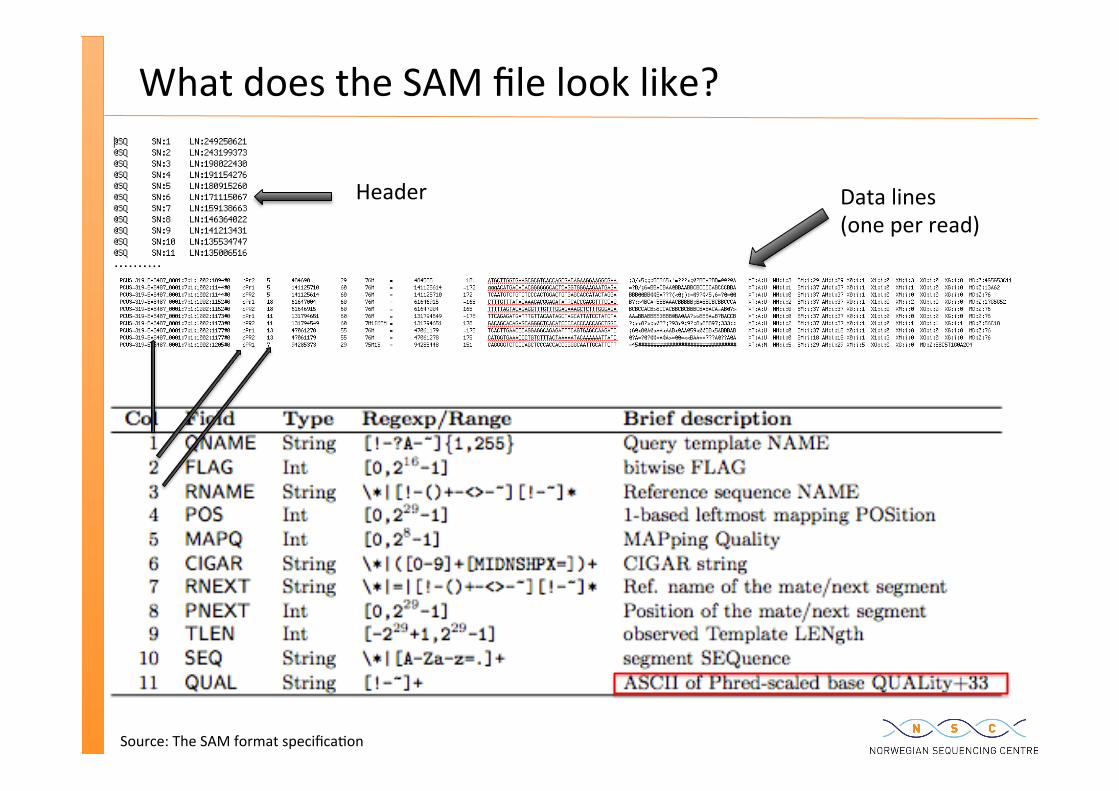
What does the SAM file look like?
Source: The SAM format specifica�on
Header Data lines (one per read)
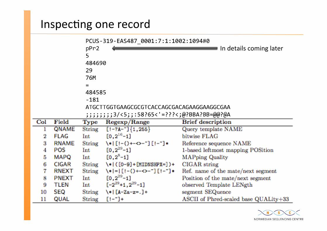
Inspec�ng one record
In details coming later
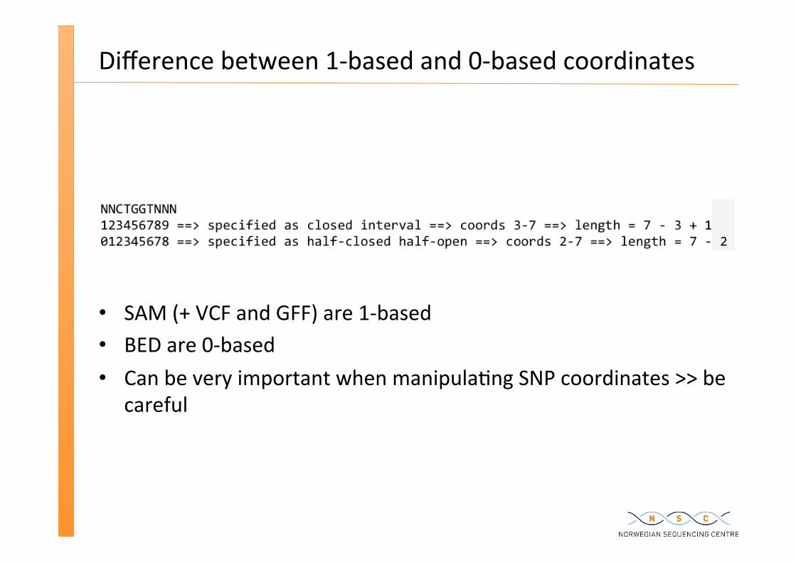
Difference between 1-‐based and 0-‐based coordinates
SAM (+ VCF and GFF) are 1-‐based BED are 0-‐based Can be very important when manipula�ng SNP coordinates >> be
careful
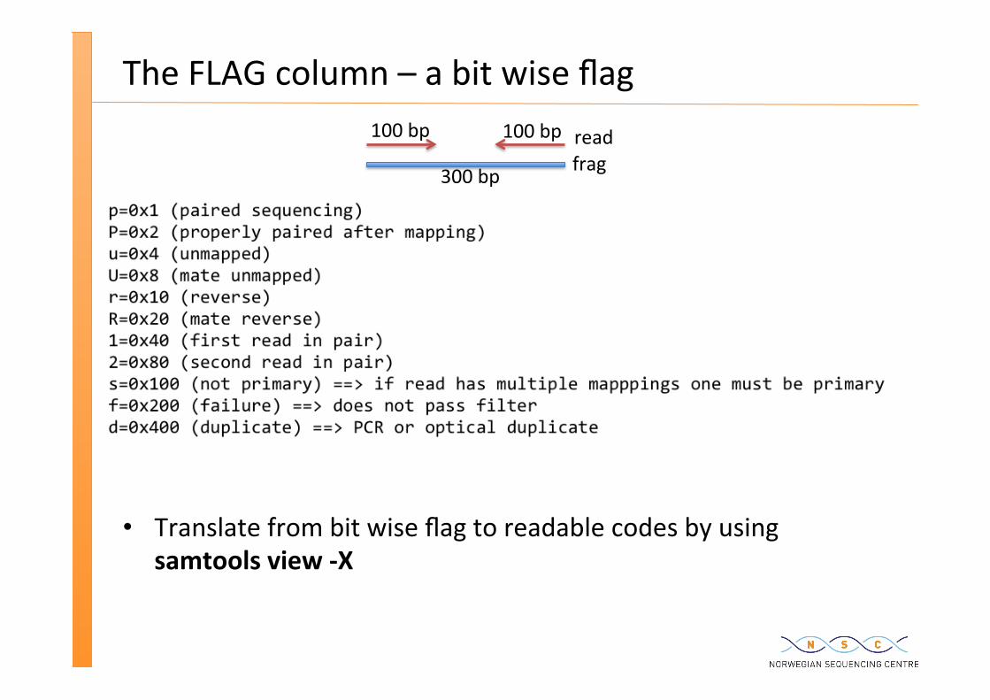
The FLAG column – a bit wise flag
Translate from bit wise flag to readable codes by using samtools view -‐X
100 bp 100 bp
300 bp frag read
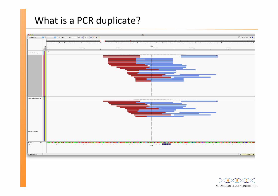
What is a PCR duplicate?
About the SAM file produced by BWA
It contains all the reads >> the Picard/GATK paradigm: informa�on is annotated (and not filtered) – unique – ambiguous – unmapped
It has a number of short comings – it takes a lot of space è convert to BAM – the mates are not fully updated on each others existence è fixmate – it is not sorted è sort – it contains PCR duplicates è mark or remove duplicates – it does not contain meta-‐data on the reads (sample, sequencer, etc)
IGV prac�cal on a basic BAM file
PRACTICAL
We take a visual look at a basic BAM file in the IGV browser
Get a feel for what a HTS dataset looks like
On the central URL: slides/igvExercise.txt
FASTQ Mapping (BWA) SAM HouseKeeping
(samtools) Variant calling
(bc�ools) Sorted BAM
VCF file
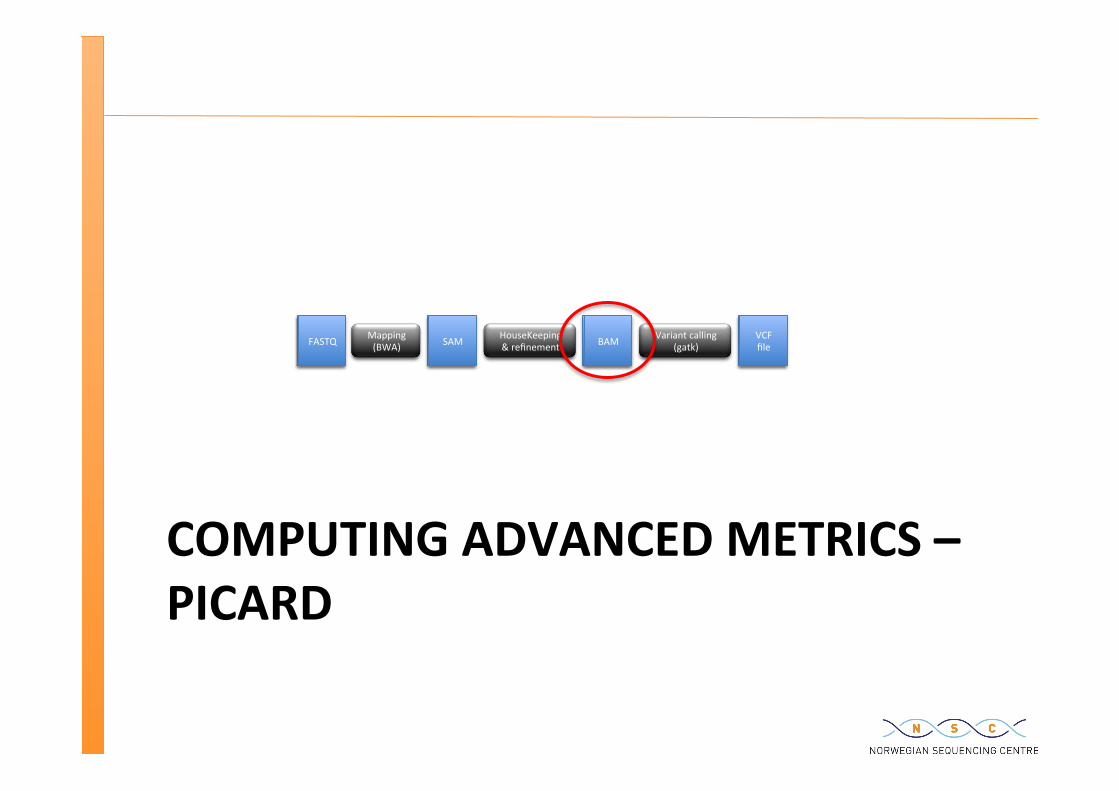
COMPUTING ADVANCED METRICS – PICARD
FASTQ Mapping (BWA) SAM HouseKeeping
& refinement Variant calling
(gatk) BAM VCF file
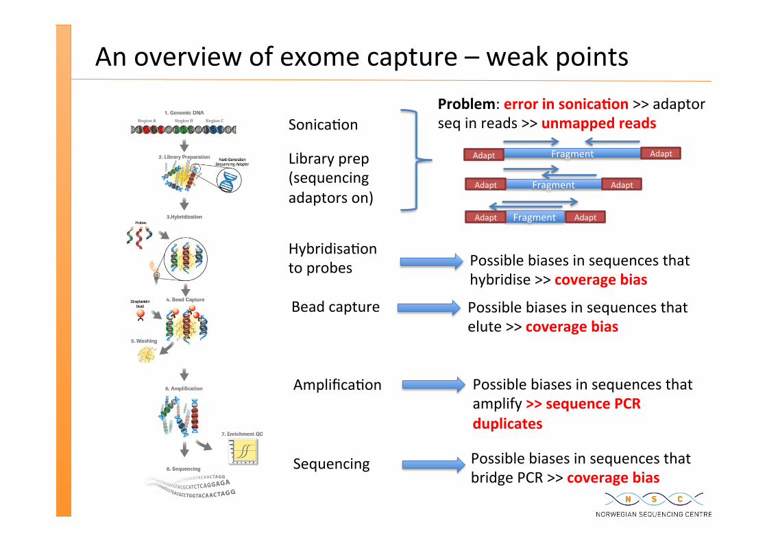
An overview of exome capture – weak points
Sonica�on
Library prep (sequencing adaptors on)
Hybridisa�on to probes
Bead capture
Amplifica�on
Fragment Adapt
Problem: error in sonica�on >> adaptor seq in reads >> unmapped reads
Possible biases in sequences that hybridise >> coverage bias
Possible biases in sequences that elute >> coverage bias
Possible biases in sequences that amplify >> sequence PCR duplicates
Possible biases in sequences that bridge PCR >> coverage bias
Sequencing
Fragment
Fragment
Adapt
Adapt
Adapt Adapt
Adapt
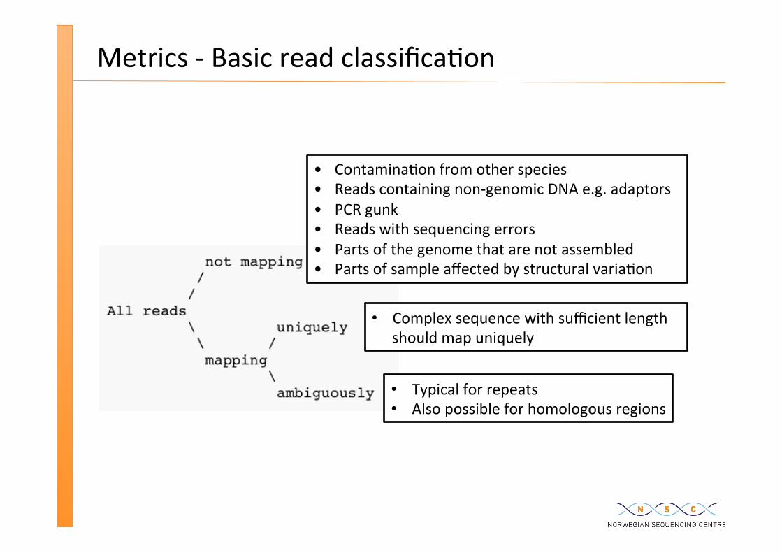
Metrics -‐ Basic read classifica�on
Typical for repeats Also possible for homologous regions
Complex sequence with sufficient length should map uniquely
• Contamina�on from other species • Reads containing non-‐genomic DNA e.g. adaptors • PCR gunk • Reads with sequencing errors • Parts of the genome that are not assembled • Parts of sample affected by structural varia�on
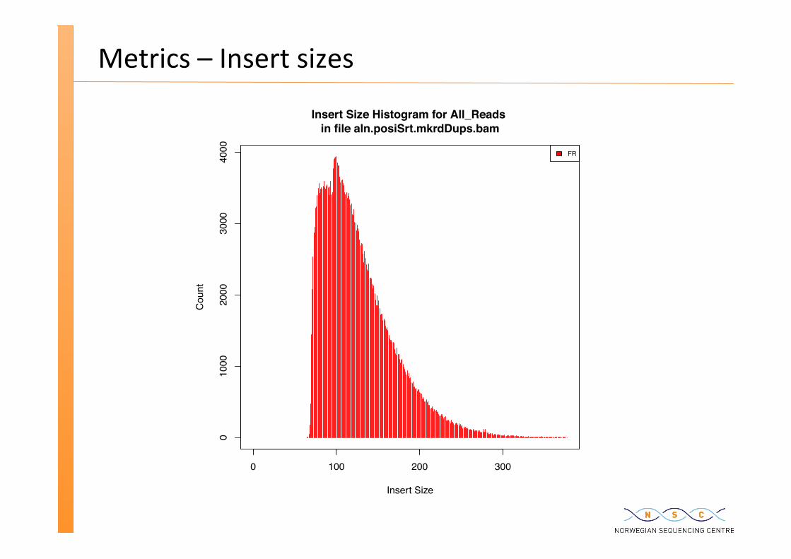
Metrics – Insert sizes
0 100 200 300
010
0020
0030
0040
00
Insert Size Histogram for All_Reads in file aln.posiSrt.mkrdDups.bam
Insert Size
Cou
nt
FR
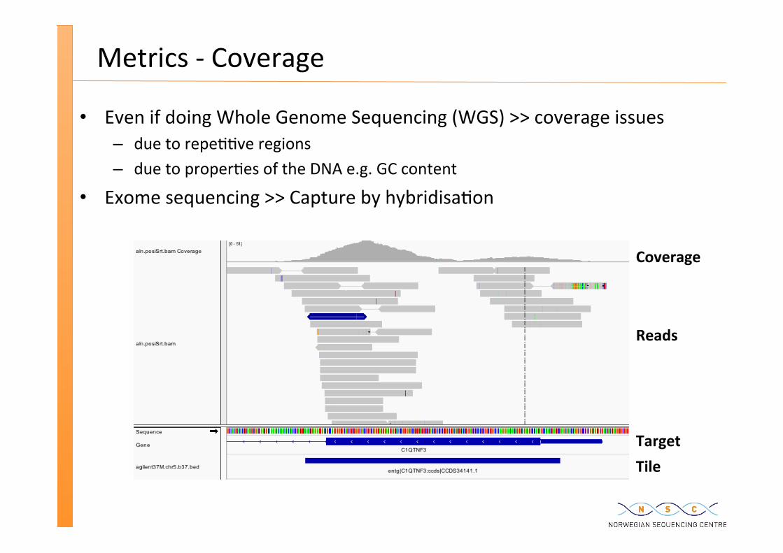
Metrics -‐ Coverage
Even if doing Whole Genome Sequencing (WGS) >> coverage issues – due to repe��ve regions – due to proper�es of the DNA e.g. GC content
Exome sequencing >> Capture by hybridisa�on
Tile Target
Reads
Coverage
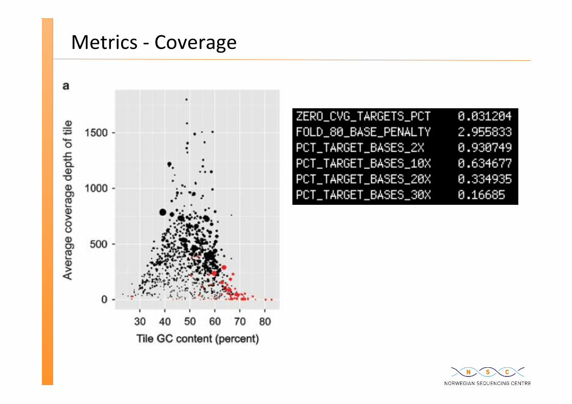
Metrics -‐ Coverage
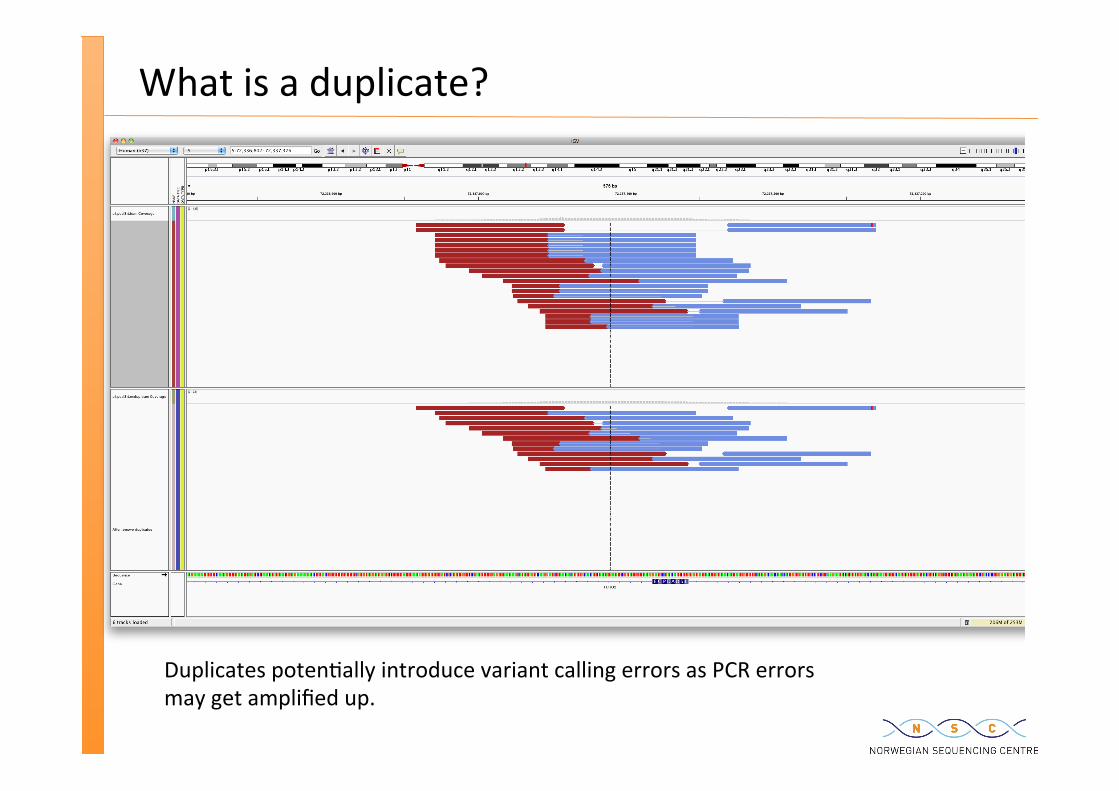
What is a duplicate?
Duplicates poten�ally introduce variant calling errors as PCR errors may get amplified up.
Calcula�ng these metrics in prac�ce
Specific Picard tools – CollectAlignmentSummaryMetrics.jar – CollectInsertSizeMetrics.jar – CalculateHsMetrics.jar
We will later take a look at this at work in a script – exerDefini�ons/04_advancedPipelineWithFuncAnnot/
04_advancedPipelineWithFuncAnnot.bash
RE-‐ALIGNMENT
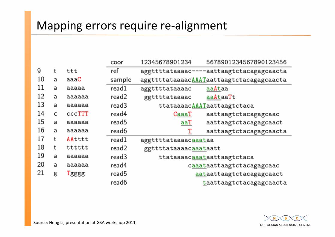
Mapping errors require re-‐alignment
Source: Heng Li, presenta�on at GSA workshop 2011
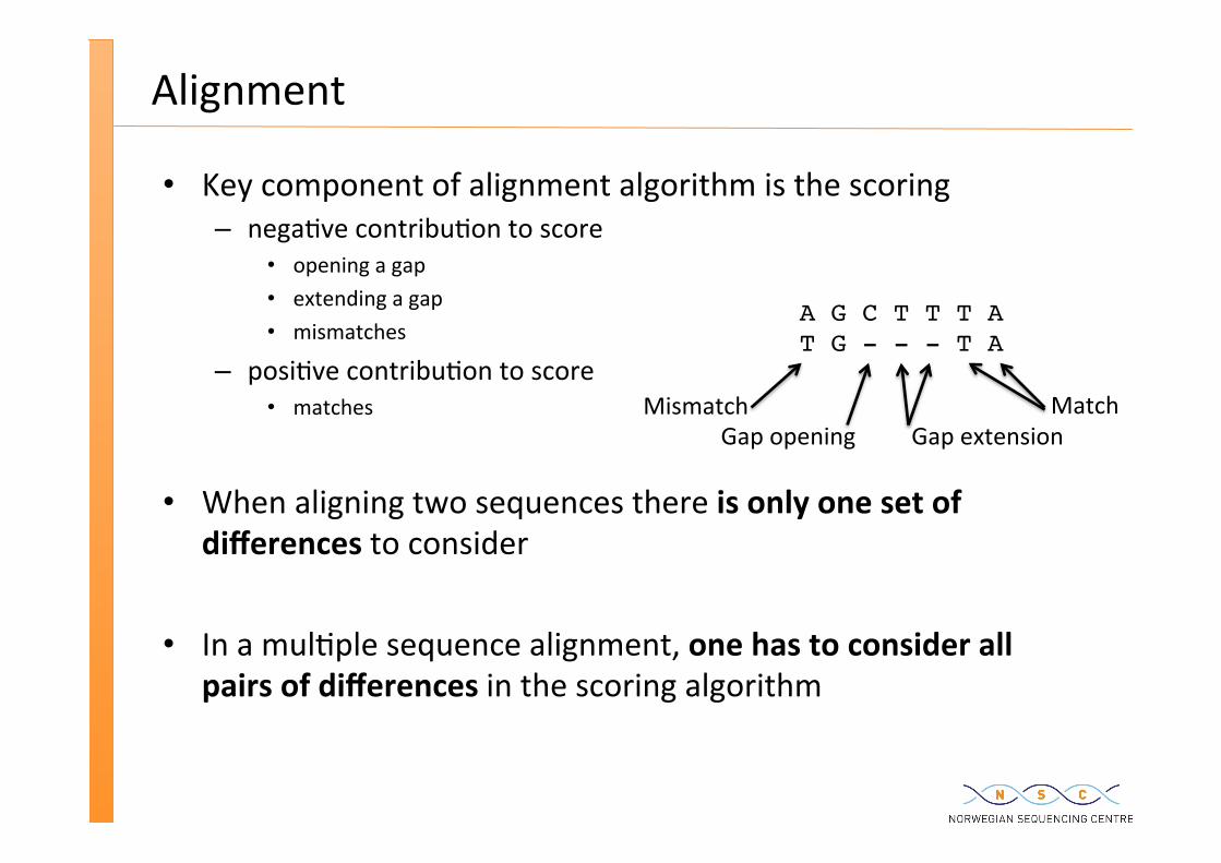
Alignment
Key component of alignment algorithm is the scoring – nega�ve contribu�on to score
opening a gap extending a gap mismatches
– posi�ve contribu�on to score matches
When aligning two sequences there is only one set of differences to consider
In a mul�ple sequence alignment, one has to consider all pairs of differences in the scoring algorithm
A G C T T T AT G - - - T A
Match Mismatch Gap opening Gap extension
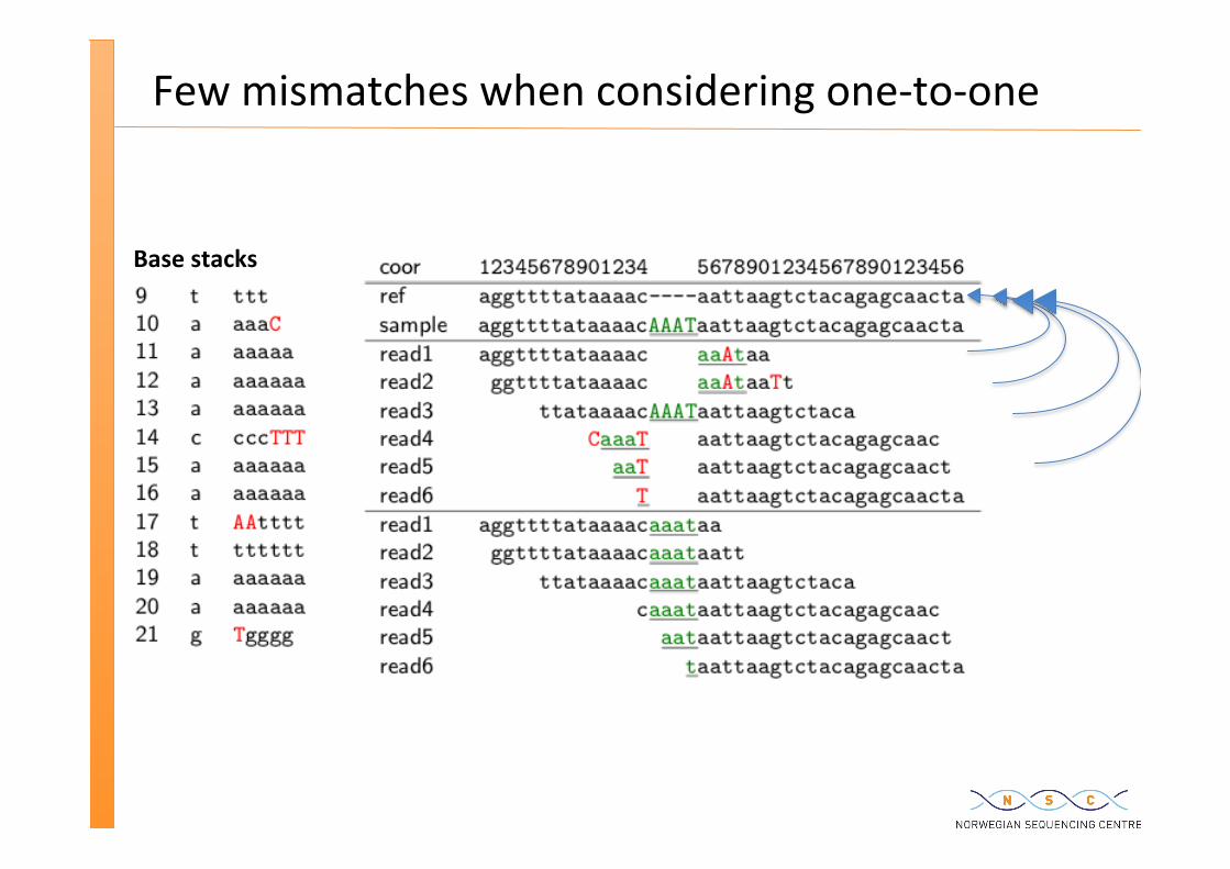
Few mismatches when considering one-‐to-‐one
Base stacks
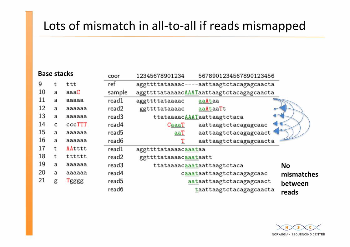
Lots of mismatch in all-‐to-‐all if reads mismapped
Base stacks
No mismatches between reads
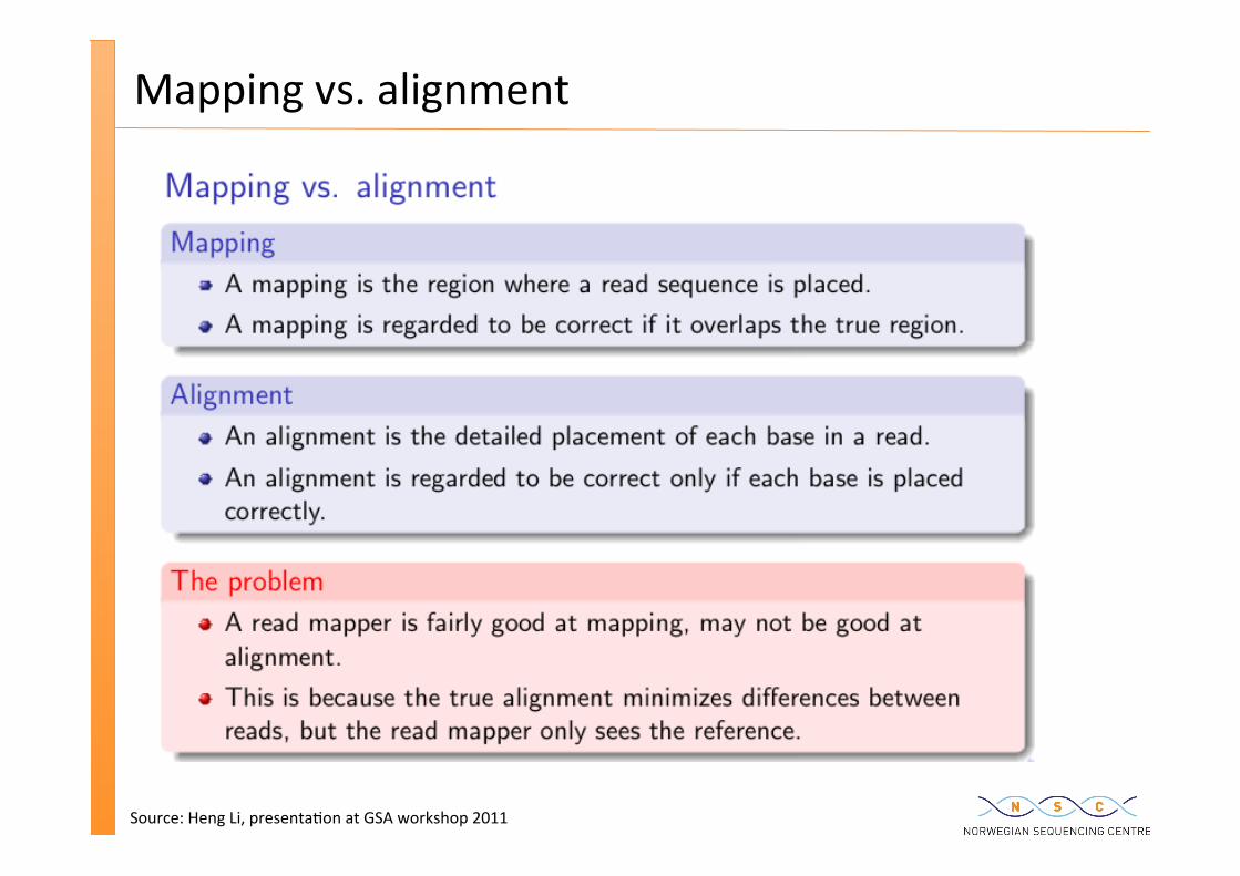
Mapping vs. alignment
Source: Heng Li, presenta�on at GSA workshop 2011
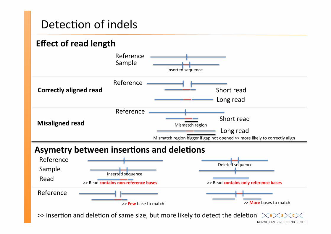
Detec�on of indels
Reference Sample
Short read Reference
Long read
Inserted sequence
Mismatch region bigger if gap not opened >> more likely to correctly align
Mismatch region
Short read Reference
Long read
Reference Sample
Inserted sequence
Deleted sequence
>> Read contains non-‐reference bases >> Read contains only reference bases
Effect of read length
Asymetry between inser�ons and dele�ons
Reference >> Few base to match >> More bases to match
Read
>> inser�on and dele�on of same size, but more likely to detect the dele�on
Misaligned read
Correctly aligned read
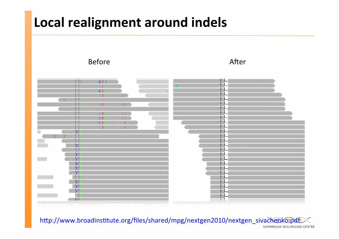
Local realignment around indels
Before A�er
h�p://www.broadins�tute.org/files/shared/mpg/nextgen2010/nextgen_sivachenko.pdf
BASE QUALITY SCORE RECALIB. (NOT CURRICULUM)
Theore�cal vs Empirical error rates / quali�es
The quali�es in the fastq file are computed using a model
This model is not perfect >> there are discrepancies between the model and the empirical error rate
We can compute a good approxima�on of the empirical error rate by iden�fying all sites where there are mismatches between the read and the reference (being careful to ignore sites with known SNPs)
We can analyse whether there are parameters of the bases that covary with the discrepancy – e.g. cycle
We can use these quan�fied covariances to recalibrate the base quali�es >> more accurate “computed quali�es” quali�es
Will help with improve the quality of the variant calling
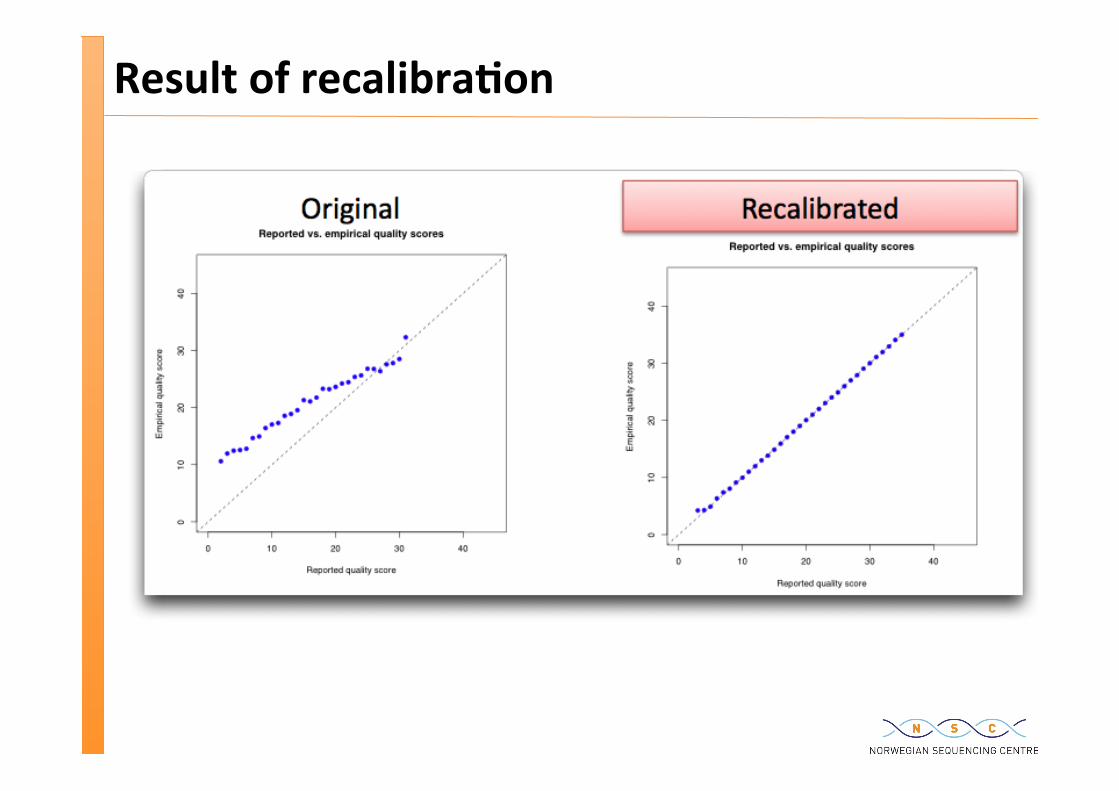
Result of recalibra�on
VCF FORMAT – MORE DETAILS
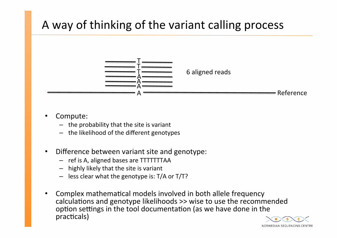
A way of thinking of the variant calling process
Compute: – the probability that the site is variant – the likelihood of the different genotypes
Difference between variant site and genotype: – ref is A, aligned bases are TTTTTTTAA – highly likely that the site is variant – less clear what the genotype is: T/A or T/T?
Complex mathema�cal models involved in both allele frequency calcula�ons and genotype likelihoods >> wise to use the recommended op�on se�ngs in the tool documenta�on (as we have done in the prac�cals)
AAAAT T T
6 aligned reads
Reference
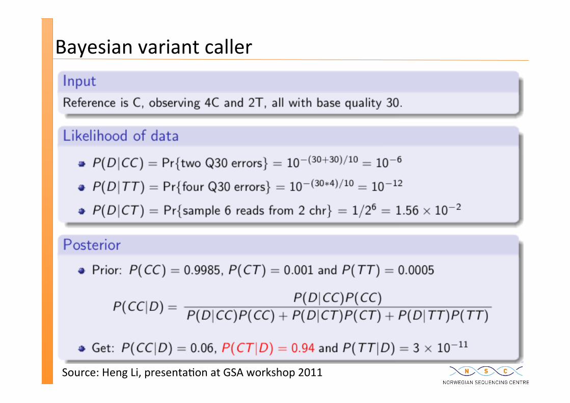
Bayesian variant caller
Source: Heng Li, presenta�on at GSA workshop 2011
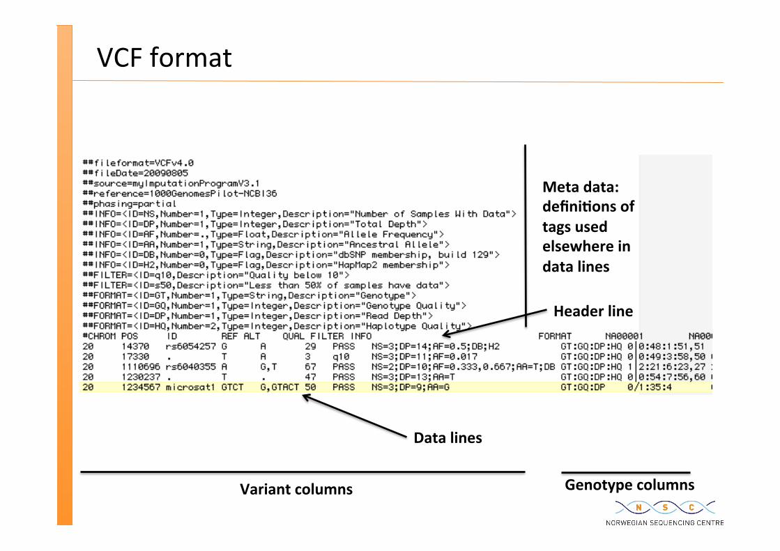
VCF format
Meta data: defini�ons of tags used elsewhere in data lines
Header line
Data lines
Variant columns Genotype columns
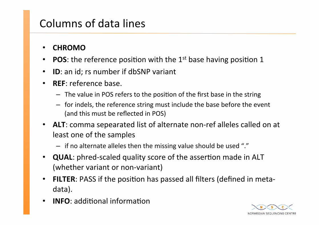
Columns of data lines
CHROMO POS: the reference posi�on with the 1st base having posi�on 1 ID: an id; rs number if dbSNP variant REF: reference base. – The value in POS refers to the posi�on of the first base in the string – for indels, the reference string must include the base before the event
(and this must be reflected in POS)
ALT: comma sepearated list of alternate non-‐ref alleles called on at least one of the samples – if no alternate alleles then the missing value should be used “.”
QUAL: phred-‐scaled quality score of the asser�on made in ALT (whether variant or non-‐variant)
FILTER: PASS if the posi�on has passed all filters (defined in meta-‐data).
INFO: addi�onal informa�on
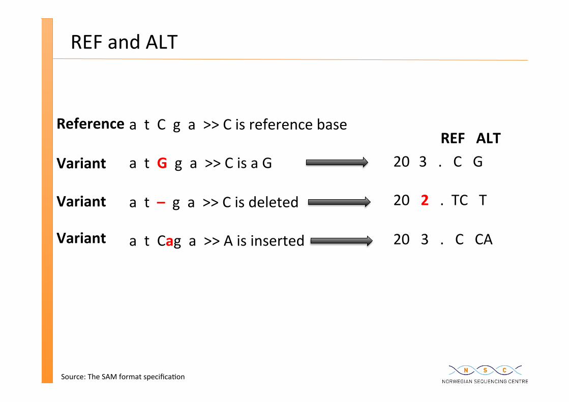
REF and ALT
Source: The SAM format specifica�on
Reference a t C g a >> C is reference base a t G g a >> C is a G a t – g a >> C is deleted a t Cag a >> A is inserted
20 3 . C G 20 2 . TC T 20 3 . C CA
REF ALT Variant
Variant
Variant
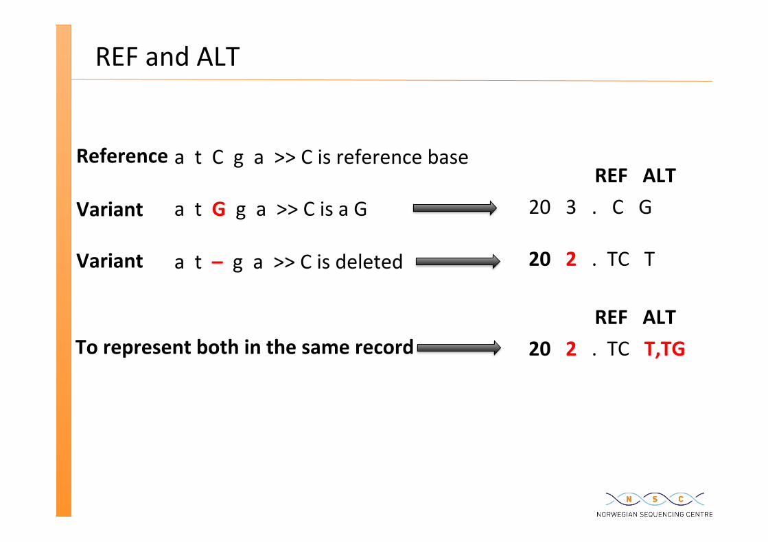
REF and ALT
Reference a t C g a >> C is reference base a t G g a >> C is a G a t – g a >> C is deleted
20 3 . C G 20 2 . TC T
REF ALT Variant
Variant
To represent both in the same record 20 2 . TC T,TG
REF ALT
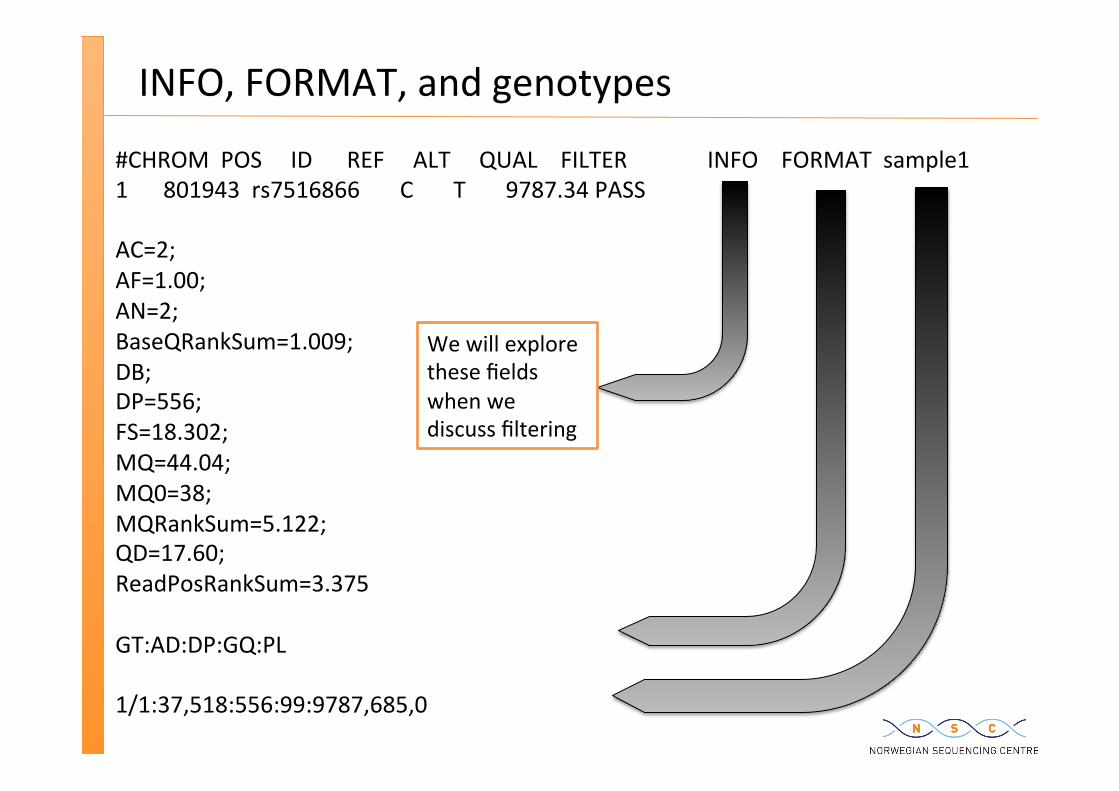
INFO, FORMAT, and genotypes
#CHROM POS ID REF ALT QUAL FILTER INFO FORMAT sample1 1 801943 rs7516866 C T 9787.34 PASS AC=2; AF=1.00; AN=2; BaseQRankSum=1.009; DB; DP=556; FS=18.302; MQ=44.04; MQ0=38; MQRankSum=5.122; QD=17.60; ReadPosRankSum=3.375 GT:AD:DP:GQ:PL 1/1:37,518:556:99:9787,685,0
We will explore these fields when we discuss filtering
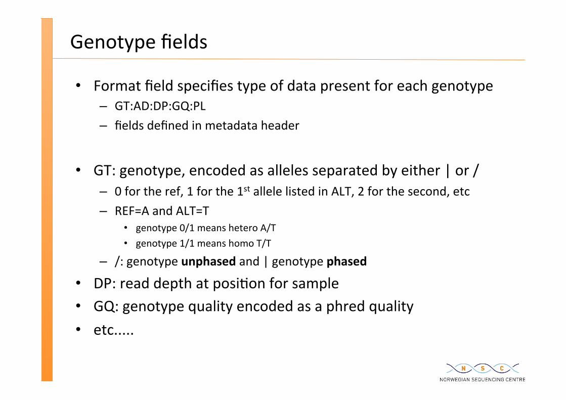
Genotype fields
Format field specifies type of data present for each genotype – GT:AD:DP:GQ:PL – fields defined in metadata header
GT: genotype, encoded as alleles separated by either | or / – 0 for the ref, 1 for the 1st allele listed in ALT, 2 for the second, etc – REF=A and ALT=T
genotype 0/1 means hetero A/T genotype 1/1 means homo T/T
– /: genotype unphased and | genotype phased
DP: read depth at posi�on for sample GQ: genotype quality encoded as a phred quality etc.....
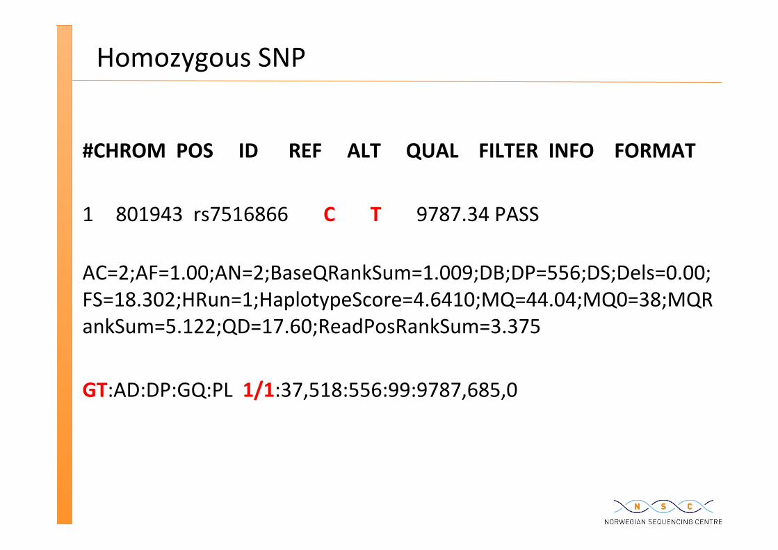
Homozygous SNP
#CHROM POS ID REF ALT QUAL FILTER INFO FORMAT 1 801943 rs7516866 C T 9787.34 PASS AC=2;AF=1.00;AN=2;BaseQRankSum=1.009;DB;DP=556;DS;Dels=0.00;FS=18.302;HRun=1;HaplotypeScore=4.6410;MQ=44.04;MQ0=38;MQRankSum=5.122;QD=17.60;ReadPosRankSum=3.375 GT:AD:DP:GQ:PL 1/1:37,518:556:99:9787,685,0
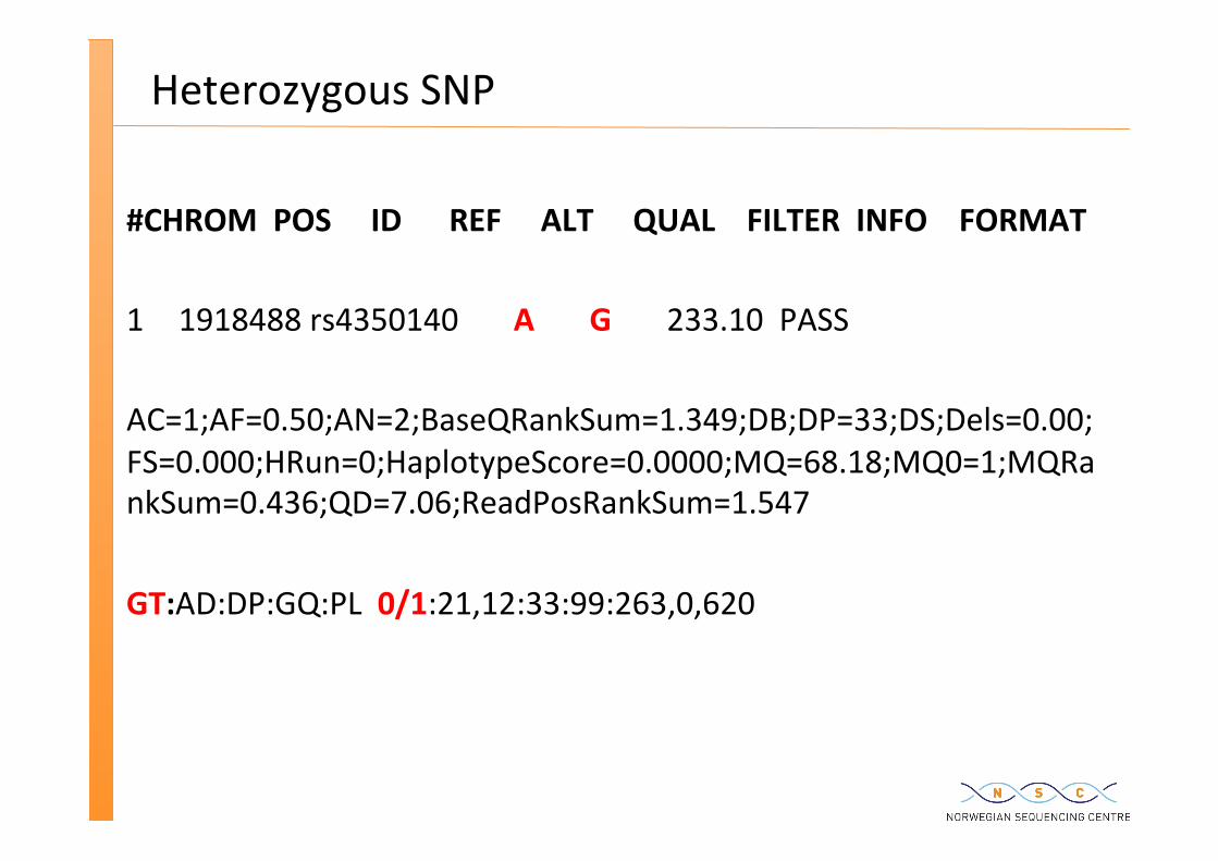
Heterozygous SNP
#CHROM POS ID REF ALT QUAL FILTER INFO FORMAT 1 1918488 rs4350140 A G 233.10 PASS AC=1;AF=0.50;AN=2;BaseQRankSum=1.349;DB;DP=33;DS;Dels=0.00;FS=0.000;HRun=0;HaplotypeScore=0.0000;MQ=68.18;MQ0=1;MQRankSum=0.436;QD=7.06;ReadPosRankSum=1.547 GT:AD:DP:GQ:PL 0/1:21,12:33:99:263,0,620
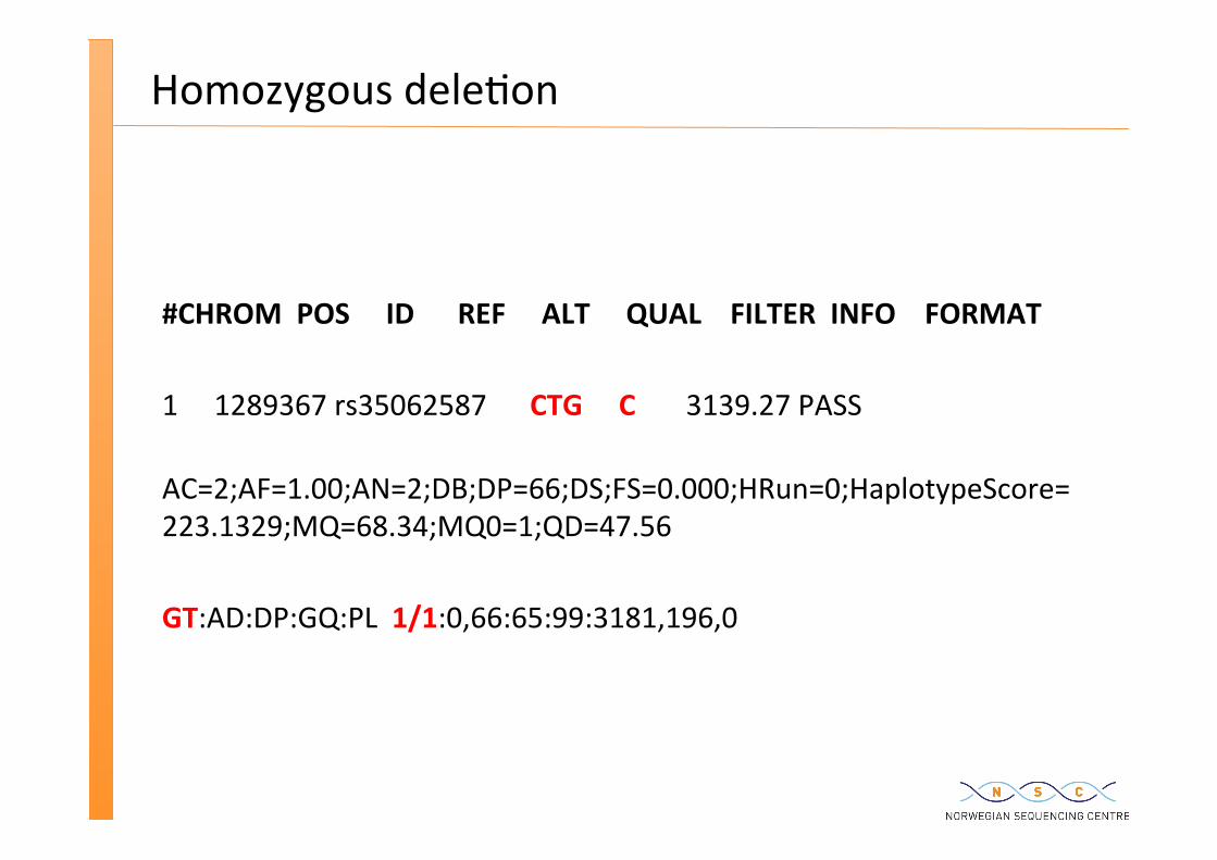
Homozygous dele�on
#CHROM POS ID REF ALT QUAL FILTER INFO FORMAT 1 1289367 rs35062587 CTG C 3139.27 PASS AC=2;AF=1.00;AN=2;DB;DP=66;DS;FS=0.000;HRun=0;HaplotypeScore=223.1329;MQ=68.34;MQ0=1;QD=47.56 GT:AD:DP:GQ:PL 1/1:0,66:65:99:3181,196,0
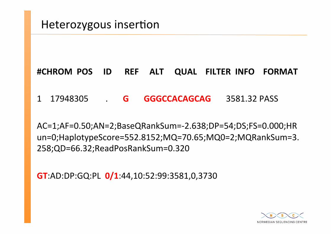
Heterozygous inser�on
#CHROM POS ID REF ALT QUAL FILTER INFO FORMAT 1 17948305 . G GGGCCACAGCAG 3581.32 PASS AC=1;AF=0.50;AN=2;BaseQRankSum=-‐2.638;DP=54;DS;FS=0.000;HRun=0;HaplotypeScore=552.8152;MQ=70.65;MQ0=2;MQRankSum=3.258;QD=66.32;ReadPosRankSum=0.320 GT:AD:DP:GQ:PL 0/1:44,10:52:99:3581,0,3730
FILTERING
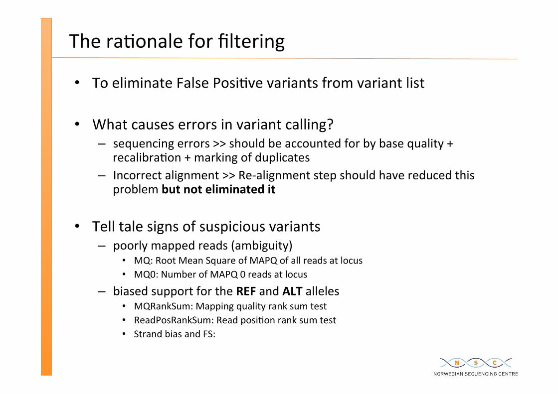
The ra�onale for filtering
To eliminate False Posi�ve variants from variant list
What causes errors in variant calling? – sequencing errors >> should be accounted for by base quality +
recalibra�on + marking of duplicates – Incorrect alignment >> Re-‐alignment step should have reduced this
problem but not eliminated it
Tell tale signs of suspicious variants – poorly mapped reads (ambiguity)
MQ: Root Mean Square of MAPQ of all reads at locus MQ0: Number of MAPQ 0 reads at locus
– biased support for the REF and ALT alleles MQRankSum: Mapping quality rank sum test ReadPosRankSum: Read posi�on rank sum test Strand bias and FS:
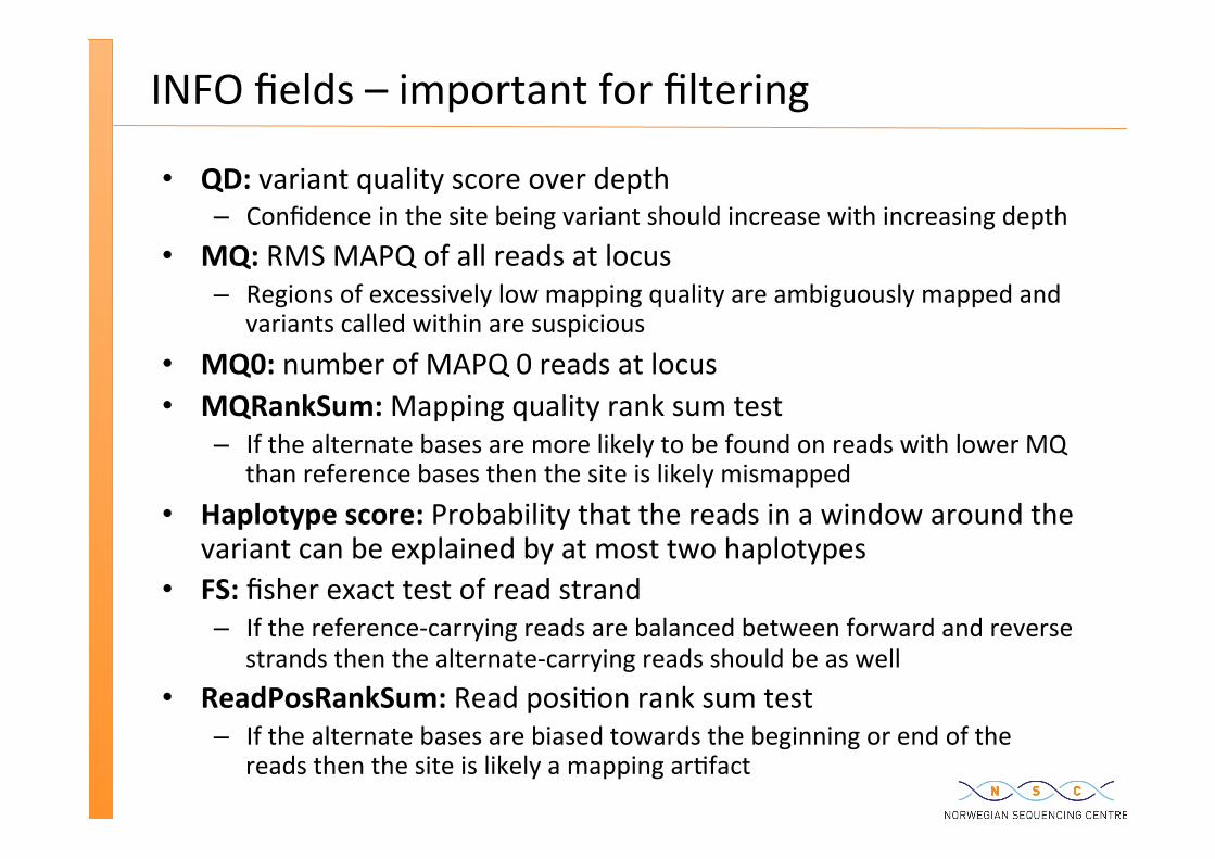
INFO fields – important for filtering
QD: variant quality score over depth – Confidence in the site being variant should increase with increasing depth
MQ: RMS MAPQ of all reads at locus – Regions of excessively low mapping quality are ambiguously mapped and
variants called within are suspicious MQ0: number of MAPQ 0 reads at locus MQRankSum: Mapping quality rank sum test – If the alternate bases are more likely to be found on reads with lower MQ
than reference bases then the site is likely mismapped Haplotype score: Probability that the reads in a window around the
variant can be explained by at most two haplotypes FS: fisher exact test of read strand – If the reference-‐carrying reads are balanced between forward and reverse
strands then the alternate-‐carrying reads should be as well ReadPosRankSum: Read posi�on rank sum test – If the alternate bases are biased towards the beginning or end of the
reads then the site is likely a mapping ar�fact
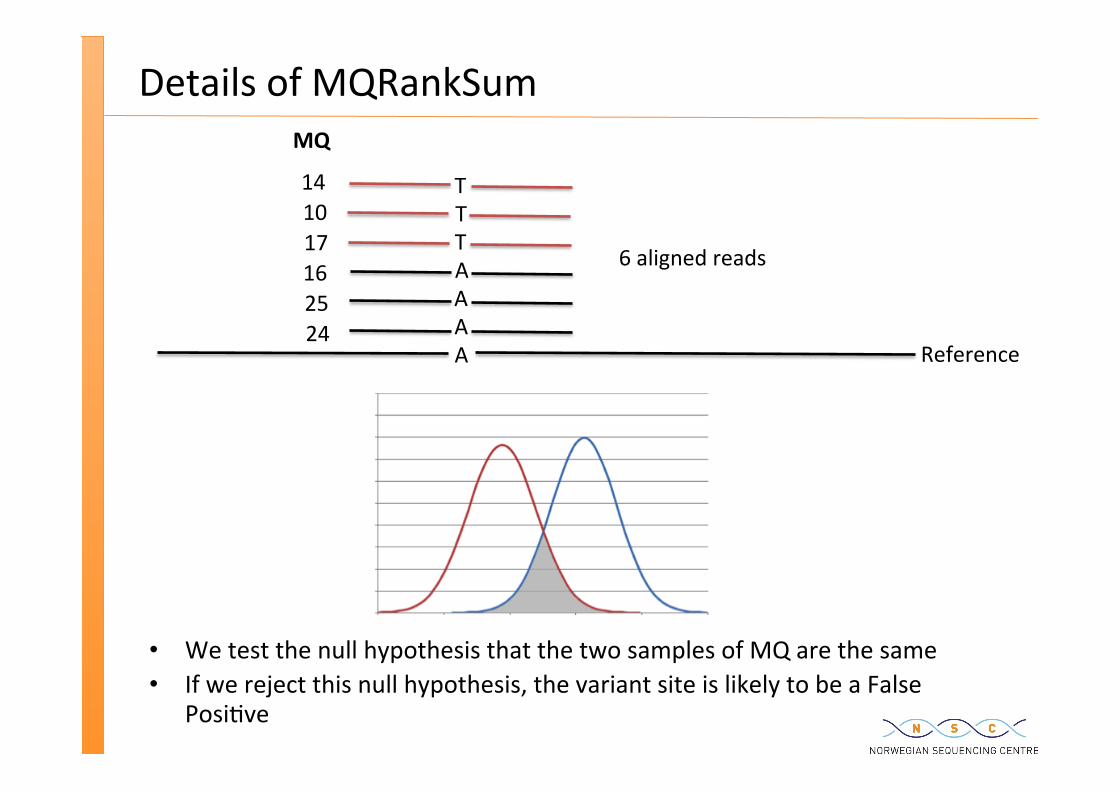
Details of MQRankSum
We test the null hypothesis that the two samples of MQ are the same If we reject this null hypothesis, the variant site is likely to be a False
Posi�ve
AAAAT
T T
6 aligned reads
Reference
MQ
10 17
14
25 24
16
ANNOTATION
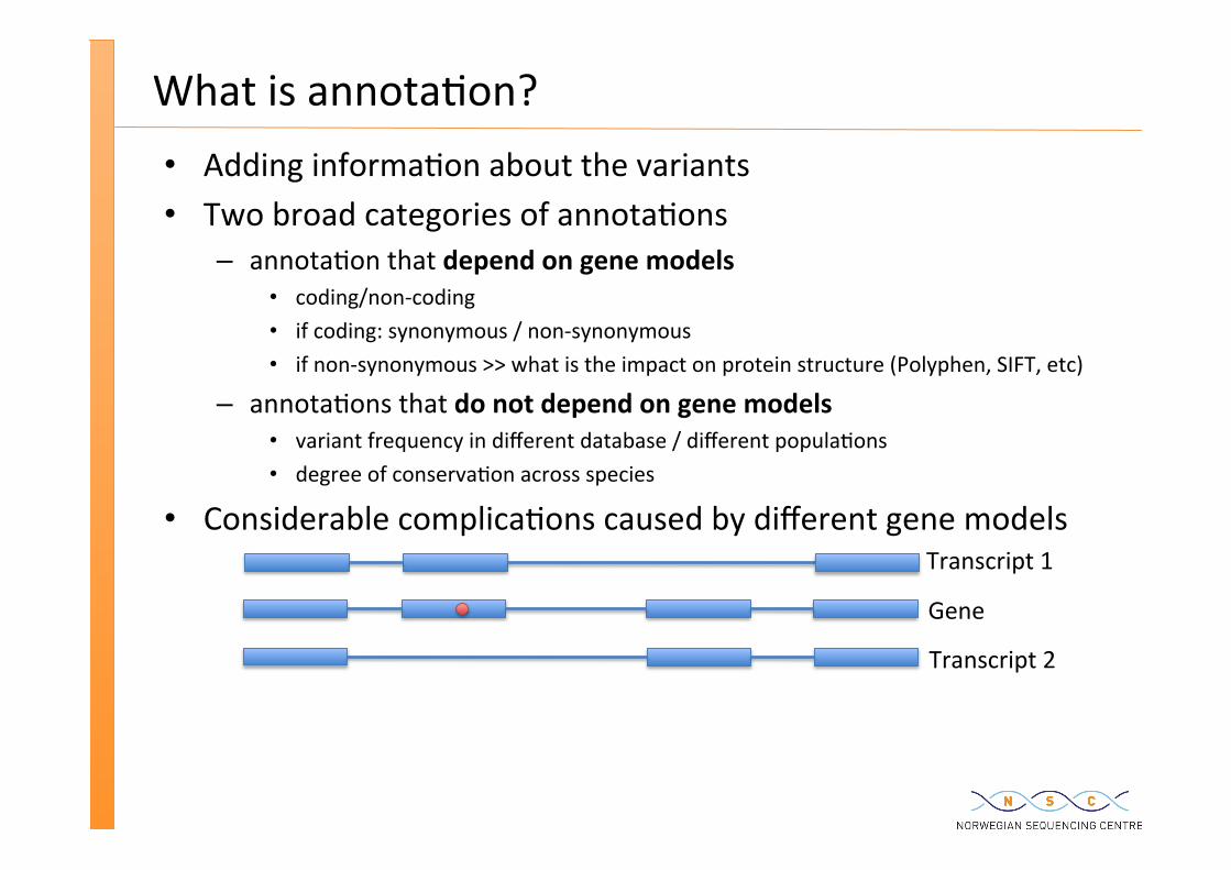
What is annota�on? Adding informa�on about the variants Two broad categories of annota�ons – annota�on that depend on gene models
coding/non-‐coding if coding: synonymous / non-‐synonymous if non-‐synonymous >> what is the impact on protein structure (Polyphen, SIFT, etc)
– annota�ons that do not depend on gene models variant frequency in different database / different popula�ons degree of conserva�on across species
Considerable complica�ons caused by different gene models Transcript 1
Transcript 2
Gene
Annota�on so�ware Two sets of so�ware – Annovar
provides a wide range of annota�ons that can be applied with one tool we have experienced some inconsistencies in the results e.g. non-‐synonymous SNPs
without polyphen score – SNPEff and dbNSFP (non-‐synoymous func�onal predic�on)
Both tested by GATK team – recommended snpEff, but with strict requirements – snpEff version 2.0.5 (not 2.0.5d) – db should be GRCh37.64 (which is the ensembl database version 64) – should use the op�on -‐onlyCoding true (using false can cause erroneous
annota�on)
GATKs VariantAnnotator to pick the highest impact.
Finally, also annotate with dbNSFP, which contains: – variant frequencies – conserva�on scores – protein func�on effect
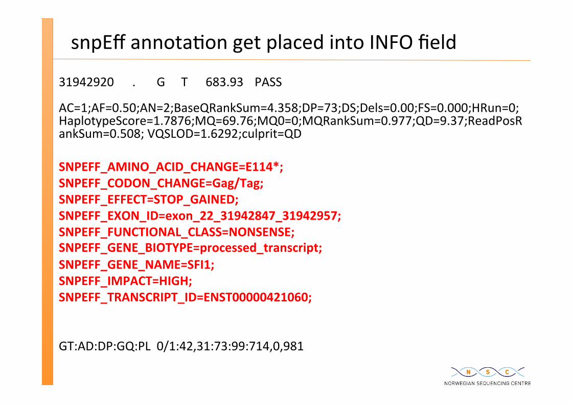
snpEff annota�on get placed into INFO field
31942920 . G T 683.93 PASS
AC=1;AF=0.50;AN=2;BaseQRankSum=4.358;DP=73;DS;Dels=0.00;FS=0.000;HRun=0;HaplotypeScore=1.7876;MQ=69.76;MQ0=0;MQRankSum=0.977;QD=9.37;ReadPosRankSum=0.508; VQSLOD=1.6292;culprit=QD SNPEFF_AMINO_ACID_CHANGE=E114*; SNPEFF_CODON_CHANGE=Gag/Tag; SNPEFF_EFFECT=STOP_GAINED; SNPEFF_EXON_ID=exon_22_31942847_31942957; SNPEFF_FUNCTIONAL_CLASS=NONSENSE; SNPEFF_GENE_BIOTYPE=processed_transcript; SNPEFF_GENE_NAME=SFI1; SNPEFF_IMPACT=HIGH; SNPEFF_TRANSCRIPT_ID=ENST00000421060;
GT:AD:DP:GQ:PL 0/1:42,31:73:99:714,0,981
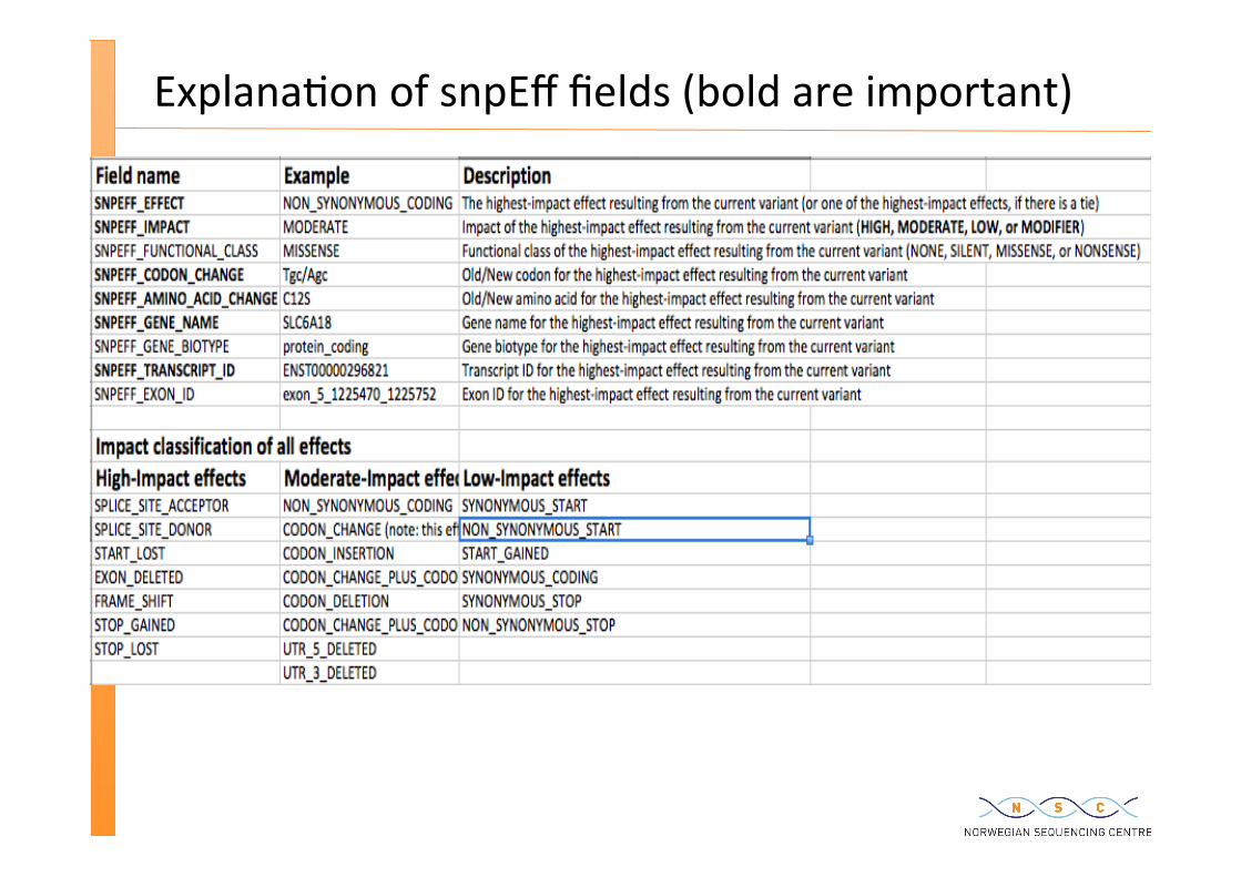
Explana�on of snpEff fields (bold are important)
All vs. top impact
SnpEff uses Ensembl gene models and annotates ini�ally with the effect in all different transcripts.
Mul�ple func�onal annota�ons for the same variant make interpreta�on difficult
One can then use GATK to pull out the TOP impact ie the most damaging effect
A second source of func�onal annota�on: dbNSFP
NSFP = Non-‐synonymous func�onal predic�on Limited to non-‐synonymous variants Has many data fields. We use only: – dbnsfpSIFT_score – dbnsfpPolyphen2_HVAR_pred – dbnsfp29way_logOdds – dbnsfp1000Gp1_AF
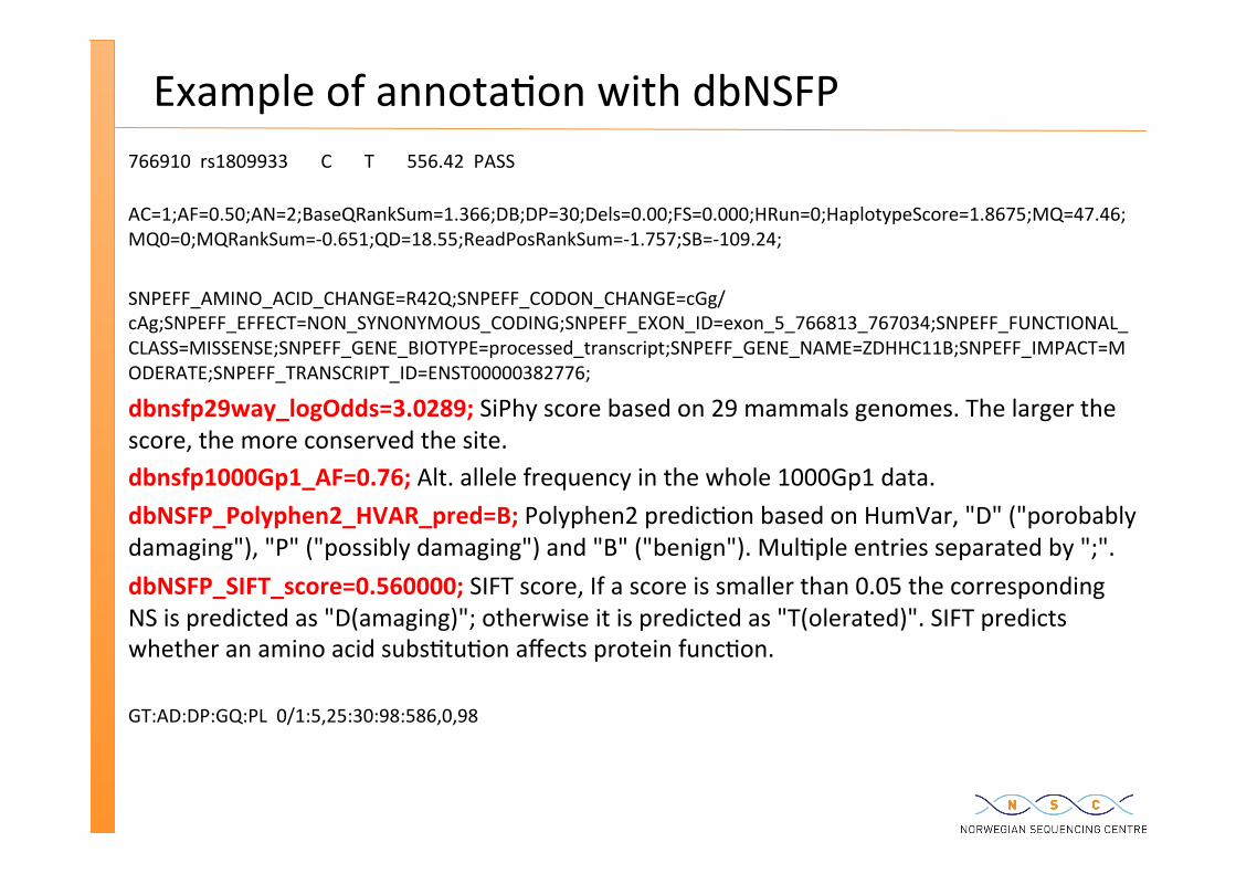
Example of annota�on with dbNSFP 766910 rs1809933 C T 556.42 PASS AC=1;AF=0.50;AN=2;BaseQRankSum=1.366;DB;DP=30;Dels=0.00;FS=0.000;HRun=0;HaplotypeScore=1.8675;MQ=47.46;MQ0=0;MQRankSum=-‐0.651;QD=18.55;ReadPosRankSum=-‐1.757;SB=-‐109.24; SNPEFF_AMINO_ACID_CHANGE=R42Q;SNPEFF_CODON_CHANGE=cGg/cAg;SNPEFF_EFFECT=NON_SYNONYMOUS_CODING;SNPEFF_EXON_ID=exon_5_766813_767034;SNPEFF_FUNCTIONAL_CLASS=MISSENSE;SNPEFF_GENE_BIOTYPE=processed_transcript;SNPEFF_GENE_NAME=ZDHHC11B;SNPEFF_IMPACT=MODERATE;SNPEFF_TRANSCRIPT_ID=ENST00000382776;
dbnsfp29way_logOdds=3.0289; SiPhy score based on 29 mammals genomes. The larger the score, the more conserved the site. dbnsfp1000Gp1_AF=0.76; Alt. allele frequency in the whole 1000Gp1 data. dbNSFP_Polyphen2_HVAR_pred=B; Polyphen2 predic�on based on HumVar, "D" ("porobably damaging"), "P" ("possibly damaging") and "B" ("benign"). Mul�ple entries separated by ";". dbNSFP_SIFT_score=0.560000; SIFT score, If a score is smaller than 0.05 the corresponding NS is predicted as "D(amaging)"; otherwise it is predicted as "T(olerated)". SIFT predicts whether an amino acid subs�tu�on affects protein func�on. GT:AD:DP:GQ:PL 0/1:5,25:30:98:586,0,98
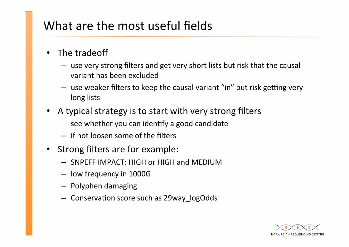
What are the most useful fields
The tradeoff – use very strong filters and get very short lists but risk that the causal
variant has been excluded – use weaker filters to keep the causal variant “in” but risk ge�ng very
long lists
A typical strategy is to start with very strong filters – see whether you can iden�fy a good candidate – if not loosen some of the filters
Strong filters are for example: – SNPEFF IMPACT: HIGH or HIGH and MEDIUM – low frequency in 1000G – Polyphen damaging – Conserva�on score such as 29way_logOdds
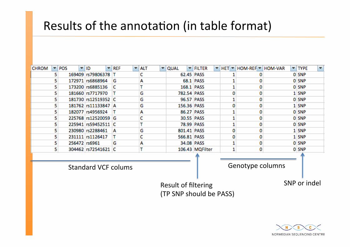
Results of the annota�on (in table format)
Genotype columns
SNP or indel Result of filtering (TP SNP should be PASS)
Standard VCF colums
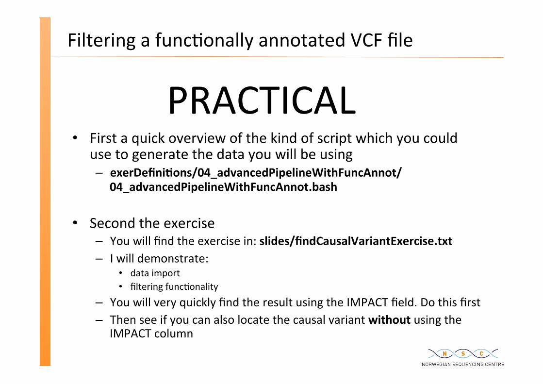
Filtering a func�onally annotated VCF file
First a quick overview of the kind of script which you could use to generate the data you will be using – exerDefini�ons/04_advancedPipelineWithFuncAnnot/04_advancedPipelineWithFuncAnnot.bash
Second the exercise – You will find the exercise in: slides/findCausalVariantExercise.txt – I will demonstrate:
data import filtering func�onality
– You will very quickly find the result using the IMPACT field. Do this first – Then see if you can also locate the causal variant without using the
IMPACT column
PRACTICAL
Concluding remarks
Concluding remarks
Appendix
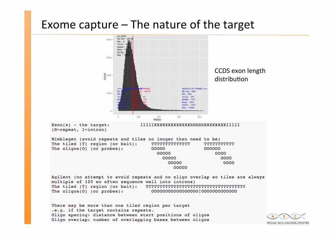
Exome capture – The nature of the target
CCDS exon length distribu�on
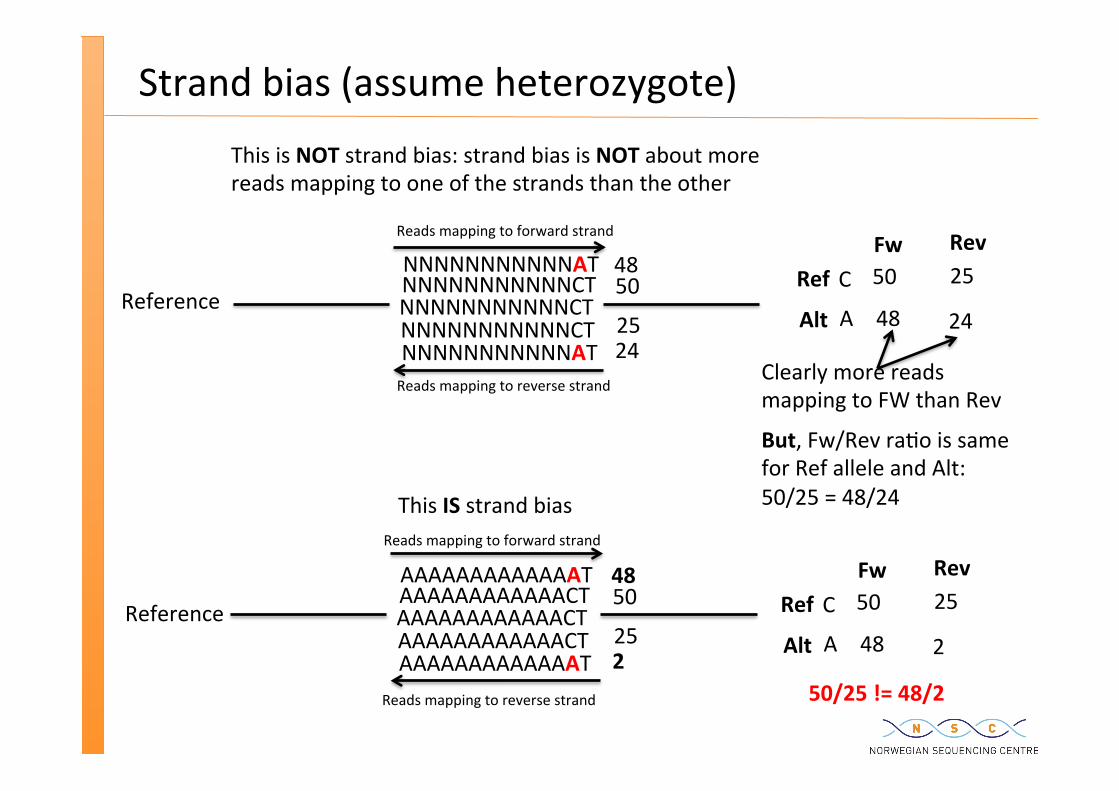
Strand bias (assume heterozygote)
AAAAAAAAAAAACT AAAAAAAAAAAACT AAAAAAAAAAAAAT
AAAAAAAAAAAACT AAAAAAAAAAAAAT
50
25
48
2
Ref
Alt
C
A
Fw Rev 50 25
48 2
Ref
Alt
C
A
Fw Rev 50 25
48 24 NNNNNNNNNNNCT NNNNNNNNNNNCT NNNNNNNNNNNAT
NNNNNNNNNNNCT NNNNNNNNNNNAT
50
25
48
24
This is NOT strand bias: strand bias is NOT about more reads mapping to one of the strands than the other
But, Fw/Rev ra�o is same for Ref allele and Alt: 50/25 = 48/24
Reference
Reads mapping to forward strand
Reads mapping to reverse strand Clearly more reads mapping to FW than Rev
This IS strand bias
50/25 != 48/2 Reads mapping to reverse strand
Reads mapping to forward strand
Reference
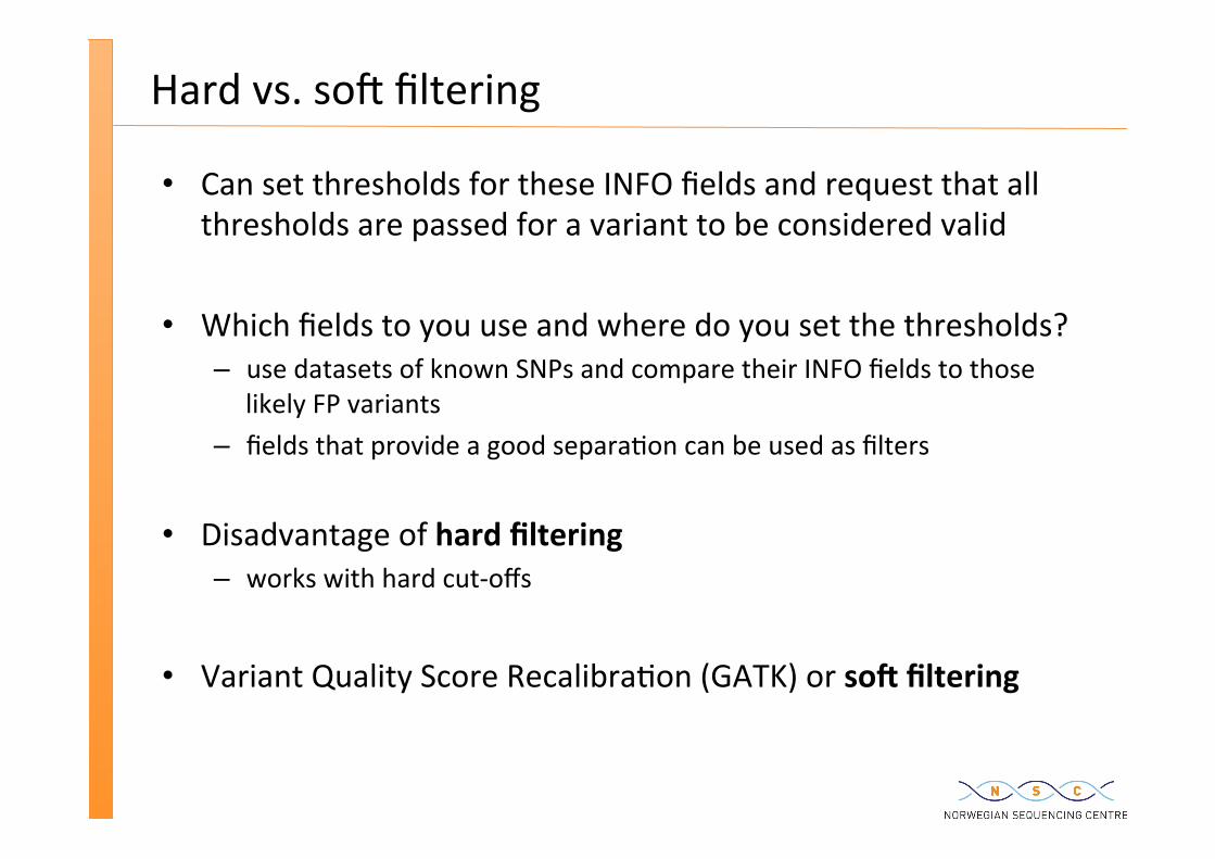
Hard vs. so� filtering
Can set thresholds for these INFO fields and request that all thresholds are passed for a variant to be considered valid
Which fields to you use and where do you set the thresholds? – use datasets of known SNPs and compare their INFO fields to those
likely FP variants – fields that provide a good separa�on can be used as filters
Disadvantage of hard filtering – works with hard cut-‐offs
Variant Quality Score Recalibra�on (GATK) or so� filtering
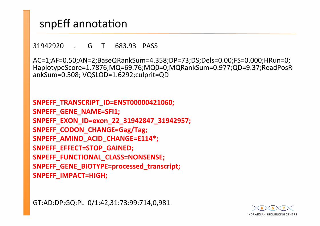
snpEff annota�on
31942920 . G T 683.93 PASS
AC=1;AF=0.50;AN=2;BaseQRankSum=4.358;DP=73;DS;Dels=0.00;FS=0.000;HRun=0;HaplotypeScore=1.7876;MQ=69.76;MQ0=0;MQRankSum=0.977;QD=9.37;ReadPosRankSum=0.508; VQSLOD=1.6292;culprit=QD SNPEFF_TRANSCRIPT_ID=ENST00000421060; SNPEFF_GENE_NAME=SFI1; SNPEFF_EXON_ID=exon_22_31942847_31942957; SNPEFF_CODON_CHANGE=Gag/Tag; SNPEFF_AMINO_ACID_CHANGE=E114*; SNPEFF_EFFECT=STOP_GAINED; SNPEFF_FUNCTIONAL_CLASS=NONSENSE; SNPEFF_GENE_BIOTYPE=processed_transcript; SNPEFF_IMPACT=HIGH;
GT:AD:DP:GQ:PL 0/1:42,31:73:99:714,0,981
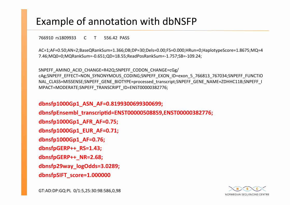
Example of annota�on with dbNSFP 766910 rs1809933 C T 556.42 PASS AC=1;AF=0.50;AN=2;BaseQRankSum=1.366;DB;DP=30;Dels=0.00;FS=0.000;HRun=0;HaplotypeScore=1.8675;MQ=47.46;MQ0=0;MQRankSum=-‐0.651;QD=18.55;ReadPosRankSum=-‐1.757;SB=-‐109.24; SNPEFF_AMINO_ACID_CHANGE=R42Q;SNPEFF_CODON_CHANGE=cGg/cAg;SNPEFF_EFFECT=NON_SYNONYMOUS_CODING;SNPEFF_EXON_ID=exon_5_766813_767034;SNPEFF_FUNCTIONAL_CLASS=MISSENSE;SNPEFF_GENE_BIOTYPE=processed_transcript;SNPEFF_GENE_NAME=ZDHHC11B;SNPEFF_IMPACT=MODERATE;SNPEFF_TRANSCRIPT_ID=ENST00000382776;
dbnsfp1000Gp1_ASN_AF=0.8199300699300699; dbnsfpEnsembl_transcrip�d=ENST00000508859,ENST00000382776; dbnsfp1000Gp1_AFR_AF=0.75; dbnsfp1000Gp1_EUR_AF=0.71; dbnsfp1000Gp1_AF=0.76; dbnsfpGERP++_RS=1.43; dbnsfpGERP++_NR=2.68; dbnsfp29way_logOdds=3.0289; dbnsfpSIFT_score=1.000000 GT:AD:DP:GQ:PL 0/1:5,25:30:98:586,0,98