Variance Estimation for Complex Surveys - Uni Trier · Variance Estimation for Complex Surveys Version: ... such as in EU-SILC, to sample households ... In each stratum a sample of

Advanced Methodology for European Laeken Indicators

Deliverable 3.1

Variance Estimation for ComplexSurveys

Version: 2011

Christian Bruch, Ralf Munnich and Stefan Zins

The project FP7–SSH–2007–217322 AMELI is supported by European Commissionfunding from the Seventh Framework Programme for Research.

http://ameli.surveystatistics.net/


II

Contributors to Deliverable 3.1

Chapter 1: Christian Bruch, Ralf Munnich and Stefan Zins, University of Trier.

Chapter 2: Ralf Munnich and Stefan Zins, University of Trier.




Main responsibility

Christian Bruch and Ralf Munnich and Stefan Zins, University of Trier

Evaluators

Internal expert: Monique Graf, Swiss Federal Statistical Office.

AMELI-WP3-D3.1

III

Aim and Objectives of Deliverable 3.1

Within the European Statistical System (ESS) more and more quality reports have to beproduced for the different surveys. One component of these reports contains informationon the accuracy of the estimates. In general, this information is based on variance com-ponents which have to be estimated from the same sample. Hence, variance estimationtechniques play an important role in modern survey statistics.

Measuring the accuracy of estimates such as totals, means or proportions generally re-quires to apply the appropriate variance estimation methodology. This allows for derivingstandard errors, confidence intervals and other similar measures as well as design effectswhich help measuring the impact of sampling designs on the outcome of the estimates. Ingeneral, two different methodologies can be applied for variance estimation of non-linearestimators, linearization and resampling methods. The efficiency of the variance estim-ators is mainly based on the properties of the point estimators as well as of the possibleskewness of the variable of interest. Further, complex sampling designs may questionthe appropriateness of the variance estimation methodology and may lead to unusualconclusions which are of major practical impact.

The methodology captured in work package 3 covers two of the most frequently en-countered problems of variance estimation in modern sample surveys. The first one isthe presence of complex sampling designs, these issues are mainly dealt with in deliv-erable 3.1. The second one is the necessity of using complex (point) estimators, e.g. ifpoverty indicators need to be estimated or their change over time, which is the main focusof deliverable 3.2 (see Munnich and Zins, 2011).

The aim of deliverable 3.1 is to give an overview of modern variance estimation meth-ods. The efficiency of the variance estimation methods can only be tested in a practicalenvironment which is achieved within a large scale simulation study.

The deliverable is structured in the following way. The introduction provides a frame-work with some much needed nomenclature and gives also a short summary on well knownvariance estimators. Thereby elements of complex sample survey designs such as strati-fication and multistage sampling are already introduced. Chapter 2 is dedicated to theproblem of variance estimator in the presence of unequal probability sampling. It is forinstance not uncommon in household surveys, such as in EU-SILC, to sample householdswith probability proportional to size, i.e. the number of persons living in the particularhousehold. Chapter 3 gives an overview on the existing resampling methods and dealswith their implementation in the presence of complex sampling designs, in particular withmulti-stage sampling and unequal selection probabilities. Chapter 4 includes the resultsfrom a small simulation study, which analyses explicitly the effects of the cluster samplingat the first stage in two-stage sampling designs. That is, we examined the influence onvariance estimates of large variations in the size of the Primary Sampling Units (PSUs),the mean value of the PSUs and the variance within the PSUs.

© http://ameli.surveystatistics.net/ - 2011


Contents

1 Introduction 2

2 Variance Estimators and their Approximation 6

2.1 Variance of the Horvitz-Thompson Estimator . . . . . . . . . . . . . . . . 6

2.2 Variance Estimation when Sampling With Replacement . . . . . . . . . . . 7

2.3 Variance Approximations . . . . . . . . . . . . . . . . . . . . . . . . . . . . 9

2.3.1 Hajek Approximation . . . . . . . . . . . . . . . . . . . . . . . . . . 12

2.3.2 Brewer Approximation . . . . . . . . . . . . . . . . . . . . . . . . . 14

2.3.3 Estimators for Variance Approximations . . . . . . . . . . . . . . . 15

3 Resampling Methods 18

3.1 Random Groups . . . . . . . . . . . . . . . . . . . . . . . . . . . . . . . . . 18

3.2 Balanced Repeated Replication . . . . . . . . . . . . . . . . . . . . . . . . 19

3.3 Jackknife . . . . . . . . . . . . . . . . . . . . . . . . . . . . . . . . . . . . . 22

3.3.1 Delete-1 jackknife for complex survey designs . . . . . . . . . . . . 23

3.3.2 Extensions of the delete-1 jackknife method . . . . . . . . . . . . . 25

3.4 Bootstrap . . . . . . . . . . . . . . . . . . . . . . . . . . . . . . . . . . . . 28

3.4.1 The Monte Carlo bootstrap . . . . . . . . . . . . . . . . . . . . . . 29

3.4.2 Bootstrap with complex survey designs . . . . . . . . . . . . . . . . 32

3.4.3 Parametric bootstrap . . . . . . . . . . . . . . . . . . . . . . . . . . 35

3.5 Discussion . . . . . . . . . . . . . . . . . . . . . . . . . . . . . . . . . . . . 35

4 Simulation Study 37

5 Summary and Outlook 46

References 46

AMELI-WP3-D3.1

Chapter 1

Introduction

In the European Statistical System quality reports gain increasingly in importance. Es-pecially the accuracy measurement of point estimators like totals, means or ratios plays amajor role. This can be done by using measures like the root mean square error or provid-ing confidence intervals for estimates. A central component of all criteria is the varianceof the point estimator which is also an accuracy criterion by itself (cf. Munnich, 2008,p. 319 f.). In practice the true value of the variance is unknown and therefore has to beestimated from the sample. The complexity of the variance estimation depends highly onthe sampling designs or parameters like the size of the Primary Sampling Units (PSUs) orthe homogeneity of the units within and between the PSUs. The aim of this deliverable isto present different variance estimation methods which can be used for different samplingdesigns and constellations of parameters.

First, we introduce a general framework which serves as the basis of our analysis. Let usconsider the finite population U of N identifiable units, so that they can be representedby integers 1,2, . . . , N, U = {1, . . . , N}. Now we want to draw a sample of n units fromU by means of random sample without replacement. A sample s can be defined by thefollowing column vector (cf. Tille, 2006, p. 8)

s = (I1, . . . , Ii, . . . , IN)T ∈ {0, 1}N , (1.1)

where

Ii =

{1 if i ∈ s0 if i /∈ s

.

Now a design specifies a probability distribution function p(.) on

Sn := {s ∈ {0, 1}n|∑

i∈U Ii = n} ,

i.e on all non-empty subsets s of n distinct units from U , (cf. Tille, 2006, p. 10 and 14)hence, ∑

s∈Sn

p(s) = 1 and p(s) ≥ 0 ∀ s ∈ Sn .

If p(.) satisfies the above condition, we call it a fixed size sampling design without re-placement, (cf. Berger, 1998a, p. 149f.). A sample S is then drawn by means of p(.)



3

such that Pr(S = s) = p(s). The probability of inclusion for the i-th element in U isdenoted by πi, with πi =

∑s3i p(s) and the second order inclusion probability πij, with

πij =∑

s3{i,j} p(s). We can now use the Horvitz-Thompson estimator

τ =∑i∈s

yi ·1

πi, (1.2)

to estimate the total τ =∑

i∈U yi.

Two basic sampling designs of this paper are stratified random sampling and two stagecluster sampling. Further sampling designs in this paper are mainly combinations of thissampling designs. In case of stratified random sampling the population is divided into Hstrata h (h = 1, . . . , H) of size Nh with N1 +N2 + ...+Nh = N . In each stratum a sampleof size nh is drawn. When the parameter of interest is a total value the variance of thisestimator is computed by:

V (τStrRS) =H∑h=1

V (τh) =H∑h=1

N2h ·(Nh − nhNh

)· σ

2h

nh, (1.3)

with

σ2h =

1

Nh − 1·Nh∑i=1

(yhi − yh)2 .

This variance can be estimated by:

V (τStrRS) =H∑h=1

N2h ·(Nh − nhNh

)· s

2h

nh, (1.4)

with

s2h =

1

nh − 1·nh∑i=1

(yhi − yh)2

(cf. Lohr, 1999, p. 99 ff.).

When a two stage cluster sampling is used the variance of the point estimator is definedby

V(θ)

= V1

[E2

(θ)]

+ E1

[V2

(θ)]

(1.5)

AMELI-WP3-D3.1

4 Chapter 1. Introduction

where E1 indicates the expected value over all possible units of the first stage and E2 theexpected value over all possible units of the second stage for a given set of units of the first

stage. V1 is the variance over the drawn PSUs and V2

(θ)

the variance over all possible

Secondary Sampling Units (SSUs) for a given set of selected PSUs (cf. Cochran, 1977,p. 275 f.).

Hence, in case of two stage cluster sampling the variance of a point estimator consists oftwo components: the first component is the variance of the several units of the first stageand the second component is the variance of the SSUs within the several PSUs (cf. Lohr,1999, p. 147).

The variance of a total value can be estimated by

V (τ2St) = N′2 ·(N′ − n′

N ′

)· s

2e

n′+N′

n′·n′∑

i=1

N′′2i ·

(N′′i − n

′′i

N′′i

)· s

2i

n′′i

(1.6)

with

s2e =

1

n′ − 1·n′∑

i=1

(τi −

τ

N ′

)2

(1.7)

and

s2i =

1

n′′i − 1

·n′′i∑

q=1

(yiq − yi)2

(cf. Lohr, 1999, p. 147).

N′

indicates the number of PSUs in the universe at stage 1 and n′

their number in thesample. N

′′i indicates the number of SSUs in the universe in a certain PSU i at stage 2

and n′′i the number of drawn SSUs in the PSU i. This procedure can easily be extended

to sampling designs with more than two stages.

The direct variance estimator of both, a two stage design with stratification at the firststage is given by:

V (τ2St) =H∑h=1

N′2h ·(N′

h − n′

h

N′h

)· s

2e

n′h

+H∑h=1

N′

h

n′h

·n′h∑

i=1

N′′2hi ·

(N′′

hi − n′′

hi

N′′hi

)· s

2hi

n′′hi

with



5

s2e =

1

n′h − 1

·n′h∑

i=1

(τhi −

τhN′h

)2

and

s2hi =

1

n′′hi − 1

·n′′hi∑

q=1

(yhiq − yhi)2

(cf. for an example of a stratified three stage design Preston, 2009, p. 228).

AMELI-WP3-D3.1

Chapter 2

Variance Estimators and theirApproximation

2.1 Variance of the Horvitz-Thompson Estimator

The variance of τ , as defined in (1.2), is calculated by

V (τ) =∑i∈U

πi(1− πi)(yiπi

)2

+ 2 ·N∑i=1

N∑j>i

(πij − πi · πj) ·yiπi· yjπj

. (2.1)

For the derivation of the above variance see Cochran (1977), p. 260. An unbiasedestimator for the variance in (2.1) is given by

V (τ) =∑i∈s

(1− πi) ·(yiπi

)2

+ 2 ·n∑i=1

n∑j>i

(1− πi · πjπij

) · yiπi· yjπj

. (2.2)

The justification of the variance estimator in (2.2) can be found in Sarndal et al. (1992),

p. 44. Although they use another notation for (2.2), V(τ) =∑∑

s1πij·(

πijπi·πj − 1

)yiyj,

with∑∑

s aij =∑

i∈s aii +∑

i∈s∑

j∈s aij and i 6= j, which is equivalent to (2.2). In caseof fixed size designs Yates and Grundy (1953), p. 257, established an alternative to thevariance estimator in (2.2). Thereafter the variance in (2.1) can also be written as

V (τ) =− 1

2

N∑i

N∑j 6=i

(πij − πi · πj) ·(yiπi− yjπj

)2

(2.3)

=N∑i=1

N∑j<i

(πi · πj − πij) ·(yiπi− yjπj

)2

,

and its unbiased estimate is given by

V (τ) =n∑i=1

n∑j<i

πi · πj − πijπij

·(yiπi− yjπj

)2

, (2.4)



2.2 Variance Estimation when Sampling With Replacement 7

(cf. Cochran, 1977, p. 260f.). For (2.4) and (2.2) to be unbiased, a necessary andsufficient condition is that πij > 0, ∀ i,l ∈ U . However, for both variance estimates tobe strictly non negative a sufficient condition is that πi · πj ≥ πij, ∀ i, j ∈ U , i 6= j, (cf.Tille, 1996, p. 179).

With the two variances estimators (2.4) and (2.2) it is possible to handle all commonsample designs. In practice, however, there are drawbacks with these estimators. First,the double sum which appears in both formulas involves a fast growing mass of termswhich demands that these variance estimators be calculated recursively, (see, Deville,1999, p. 194). Second, the second order inclusion probabilities πij are difficult to obtainfor most samples designs applied in practice. Only in rare cases with simple schemes theyare easily calulated, e.g. for a simple random sample (SRS) design without replacement(WoR) the πijs are given by

πij =

n

Ni = j ∧ i, j ≤ N

n · (n− 1)

N · (N − 1)else.

. (2.5)

The probabilities result from the hypergeometric distribution, i.e. the number of samplesincluding the i-th element

(N−1n−1

)respectively the i-th and j-th element

(N−2n−2

)divided by

the number of all possible samples(Nn

). Inserting the above inclusion probabilities into

(2.4) yields

V (τ) = N2 ·N∑i

N∑j<i

(n2

N2− n · (n− 1)

N · (N − 1)

)·(

yin/N

− yjn/N

)2

(2.6)

= N2 · N − nN · n

· 1

N − 1· 1

N·N∑i

N∑j<i

(yi − yj)2

= N2 ·1N·∑N

i=1(yi − 1N·∑N

j=1 yj)2

n· N − nN − 1

= N2 ·σ2y

n· N − nN − 1

,

where σ2y denotes the variance of variable y, (cf. Munnich, 2005, p. 55). Substituting σ2

y

by a suitable estimate σ2y, in case of SRS by 1

n−1·∑n

i=1(yi − 1n·∑n

j=1 yj)2, leads to the

variance estimate V (τ).

2.2 Variance Estimation when Sampling With Re-

placement

To avoid the calculation of the double sum in (2.4) or (2.2) in the presence of morecomplex designs different approximations can be found in the literature that only useπi but dispense with the πij, (cf. Berger and Skinner, 2004). One way to evadethe computation of this large number of cross-products is to use variance estimation for

AMELI-WP3-D3.1

8 Chapter 2. Variance Estimators and their Approximation

samples drawn with replacement. Thus, we treat the sample as it would have been drawnby more simple design than the true one. The estimation of τ from a sample drawn withreplacement can be done by the Hansen-Hurwitz estimator, (see Sarndal et al., 1992,p. 51f.).

τHH =1

n

n∑i=1

Zi , (2.7)

where Zi is a random variable such that

Zi =ykpk

that is, if the k-th element is selected in the i-th draw and pk is the selection proabilityof the k-th element. Further, we have the following relationship between the inclusionprobability πk and pk

πk = 1− (1− pk)n ,

= npk +∞∑l=2

(n

k

)(−pk)l ,

and if pk is small, which is reasonable if N is large, then πk.= npk. It follows that

∀ i = 1, . . . , n; Pr

(Zi =

ykpk

)= pk; k = 1, . . . , N .

The estimator in (2.7) is unbiased for the population total τ , becauseE(Zi) =

∑k∈U

ykpk· pk = τ and its variance is

V (τHH) =∑k∈U

(ykpk− τ)2

· pk ·1

n. (2.8)

An unbiased estimator of the variance in (2.8) is given by

V (τHH) =1

n · (n− 1)

n∑i=1

(Zi − τHH)2 , (2.9)

the proof of (2.8) and (2.9) can be found in Sarndal et al. (1992), p. 52. The varianceestimate in (2.9) can now be used to obtain a simplified variance estimation for (1.2), (cf.Sarndal et al., 1992, p. 422)

V0 (τ) =1

n · (n− 1)·∑k∈s

(ykpk− τ)2

, (2.10)

where pk is taken as pk = πkn

for k ∈ s. By using (2.10) instead of (2.4) or (2.2) wecalculate the variance estimator as if the sample was drawn with replacement, whereasit was actually drawn without replacement. But this computational simplification thatresults from getting rid of the πij has the drawback that V0 will not be without bias for



2.3 Variance Approximations 9

V (τ), (see Sarndal et al., 1992, p. 422). However, this bias which is for any fixed samplesize design given by

E(V0(τ)

)− V (τ) =

n

n− 1· (V0(τ)− V (τ)) , (2.11)

with V (τ) given in (2.1) or (2.3), will be positive in cases where sampling without re-placement results in a lower sampling variance than sampling with replacement, as it isthe case for SRS. Thus, the use of (2.10) will lead to the construction of over conservativeconfidence intervals, whereas for unequal proability sampling this need not to be the case,(cf. Gabler, 1990, p. 64f.). A sufficient conditon for V0(τ)− V (τ) to be nonnegative is

πij ≥ πi · πj · (1−1

n) , ∀ i,j ∈ U , i 6= j (2.12)

which can be seen from rewriting (2.8) in following way

V (τHH) =N∑k=1

y2k

npk− τ 2

n=

1

n

N∑k=1

N∑l<k

(ykpk− ylpl

)2

pk · pl , (2.13)

having in mind that pk = πkn

it follows that (2.13) is always greater than (2.3) if condition(2.12) is met, e.g. in cases of SRS WoR.

Although condition (2.12) is sufficient, it is not a necessary one. A weaker condition, yetstill not a necessary one, is given be Gabler (1990), p. 69f., which states that if

N∑k=1

min1≤l≤N

πklπl≤ n− 1 ,

then V0(τ) ≥ V (τ), (see also Gabler, 1984, for another sufficient condition).

Thus, we conclude that in some cases (2.9) might serve as an easy to compute estimatefor an upper bound for the sampling variance when sampling without replacement. Thissimplification is, however, limited by the fact that we need to know the πij’s to be surethat (2.8) is greater than (2.1) or (2.3).

2.3 Variance Approximations

To begin of this section we start with an alternative formulation for the variance of theHorvitz-Thompson estimator for fixed sample sizes (2.3), (cf. Brewer, 2003, p. 149).This approch will lead to a first approximation of (2.3) and show to what extent approx-imations of the second order inclusion probabilities are needed. First we begin with somegeneral properties of the inclusion probabilities, which should be respected by proposedvariance approximations, (cf. Tille, 1996, p. 184):∑

i∈Ui 6=j

πij = πj · (n− 1) (2.14a)

AMELI-WP3-D3.1

10 Chapter 2. Variance Estimators and their Approximation∑j∈U

∑i∈Ui 6=j

πij = n · (n− 1) (2.14b)

∑j∈U

∑i∈Ui 6=j

πjπi = n2 −∑j∈U

π2j (2.14c)

∑i∈Ui 6=j

(πiπj − πij) = πj(1− πj) (2.14d)

Now we may rewrite (2.3) in the following way,

V (τ) =1

2

N∑i=1

N∑j 6=i

(πi · πj − πij) ·(yiπi− τ

n

)2

−(yjπj− τ

n

)2

(2.15)

=N∑i=1

N∑j 6=i

(πi · πj − πij) ·(yiπi− τ

n

)2

−N∑i=1

N∑j 6=i

(πi · πj − πij)(yiπi− τ

n

)·(yjπj− τ

n

),

and by relation (2.14d)

V (τ) =N∑i=1

πi(1− πi) ·(yiπi− τ

n

)2

(2.16)

−N∑i=1

N∑j 6=i

(πi · πj − πij)(yiπi− τ

n

)·(yjπj− τ

n

).

The first term in (2.16) equals (2.9) for pk = πk/n with a finite population correction term(1−πi) and constitutes the major part of the variance of τ (cf., Brewer, 2003, p. 149f.).The importance of the second term in (2.16) depends on the sampling design p(.). Forthe second term to be negligiable compared to the first term, p(.) must be of the formthat πij ≈ πi · πj. For example this is justifiable in case of SRS, (see (2.5)). However, ifthe second term in (2.16) is expected to become important one can look for more suitableapproximations of πij, which lead to proxy variances of τ having the simple form of thefirst term in (2.16). This will be the main concern for rest of the section. To do so westart by considering Poisson sampling.

Poisson sampling is a design for which the variance of (1.2) can be derived as easily as forthe Hansen-Hurwitz estimator, where only the πi’s have to be known. Because in Poissonsample all elements of the random vector s in (1.1) are independent random variables.Poisson sampling is defined by

ppoiss(s) =∏i∈s

pi∏U\s

1− pi ,

with numbers 0 ≤ pi ≤ 1∀ i ∈ U (see Hajek, 1981, p. 54). Poisson sampling has arandom sample size n, with E(n) =

∑Ni=1 pi and V(n) =

∑Ni=1 pi(1− pi). Further we have




first-order inclusion probabilities, πi = pi ∀i ∈ U and second-order inclusion probabilitiesπij = pipj i, j ∈ U , i 6= j. Thus, if s is a sample drawn after ppoiss(.), then

Vpoiss(τ) = Vpoiss

(∑i∈s

yiπi

)=∑i∈U

y2i

π2i

· πi(1− πi) , (2.17)

where Vpoiss denotes the variance under the design ppoiss(.). Note that (2.17) containsalso πi because it is the variance of estimator (1.2) computed under Poisson sampling,(cf. Deville and Tille, 2005, p. 573). To have a fixed sample size we make ppoiss(.) aconditional Poisson sampling design given that its sample size n is fixed to n. Heuristicallywe can describe such a fix size Poisson sampling design as

ppoiss(s|n = n) =ppoiss(s)

P (s ∈ Sn),

where ppoiss(s|n = n) = 0 if s /∈ Sn and P (s ∈ Sn) denotes the probability under designppoiss that the size of s is n (see Berger, 2004b, p. 454). The problem connected withthe conditioning on P (s ∈ Sn) is to reevaluate the πi’s. They can be computed exactly(see Hajek, 1981, chapter. 14), but in Hajek (1964, p. 1508ff) it is shown that we canapproximate πi by πi.

We may then write for the variance of τ

V(τ) = Vpoiss (τ |n = n) ,

(cf. Matei and Tille, 2005, p. 548). If we assume that through Poisson sampling thecouple {τ , n} is bivariate normal distributed (cf. Deville and Tille, 2005, p. 573) then,by exploiting the linear relation between τ and n, it is possible to write

Vpoiss (τ |n = n) = Vpoiss(τ + (n− n) · β) , (2.18)

where

β =Covpoiss(n, τ)

Vpoiss(n),

and

Covpoiss(n, τ) =∑i∈U

πi(1− πi) ·yiπi,

Vpoiss(n) =∑i∈U

πi(1− πi) .

If we define bi = πi(1− πi) we get the following variance approximation formula

Vapprox (τ) =∑i∈U

bi · ε2i , (2.19)

where

εi =yiπi− β.

AMELI-WP3-D3.1


Approximation (2.19) is valid for the class of maximum entropy designs, which are designsthat maximise the quantity

−∑s∈S

p(s) log p(s) ,

under condition πi =∑

s3i p(s), which is met by conditional Poisson samplign p(.) (cf.Matei and Tille, 2005).

Depending on the choice of bi there exist numerous variants of approximation (2.19). Ananalysis of the literature on different values of bi can be found in Matei and Tille (2005).

2.3.1 Hajek Approximation

Hajek (1964), p. 1509, proposed the following relation between the probabilities πi andπij

πiπj − πij = d−1 · πi (1− πi) · πj · (1− πj) [1 + o(1)] , (2.20)

where d =∑

i∈U πi · (1 − πi) and o(1) → 0 if d → ∞. The relation above is vaildfor rejective sampling, which he defines as a conditional Poisson sampling or conditionalsampling with replacement, (cf. Hajek, 1981, p. 66f.). Thus, we can write:

πij ≈ πiπj ·(1− (1− πi) · (1− πj) · d−1

)1 ≤ i 6= j ≤ N . (2.21)

Inserting (2.21) into (2.3) gives the following approximation for V (τ)

VHaj(τ) =∑i∈U

πi(1− πi) ·(yiπi−B

)2

, (2.22)

where

B =

∑i∈U

yiπi· πi(1− πi)∑

i∈U πi(1− πi).

Now the right-hand side of formula (2.20) may be approximated by the prodcut cicj where

ci = πi(1 − πi) ·√d−1

. But because this does not satisfy the relation (2.14d) let ci be

set to ci = πi(1 − λi) ·√dλ−1

and dλ =∑N

j=1 πj(1 − λj). Hajek (1981), p. 27, gives anapproximation of the πi(1 − λi) terms, which can be described, in line with the generalapproximation in (2.19), in the following way

HAJEKb∗i = πi(1− λi) = πi(1− πi) ·

[1− πi(1− λi)

dλ

]−1

. (2.23)

A value for πi(1 − λi) is then obtained by iteration. For the first iteration insertingπi(1− λi) = πi(1− πi) on the right hand side. The obtained value is then again instertedon the right hand side of (2.23), this process is repeated until the results become stableas πi(1− λi) converges to πi(1− πi) (cf. Hajek, 1981, p. 76). As a compromise between




simplicity and precision Hajek (1981) proposed for small πi’s the following approximationfor bi

HAJEKbi = πi(1−n− 1

nπi) . (2.24)

For πi = nN∀i ∈ U (2.22) becomes the standard variance estimator (2.6), (cf. Berger,

2003, p. 9 ). Note that ifτ

nis substituted by B in (2.22) equals the first term in (2.16).

Furthermore, Berger (1998a), showed that (2.21) can also be used for a class of highlyrandomized or high entropy sampling designs (cf. Berger, 2004a, p. 307), which includesamongst others the RaoSampford sampling design (see, Sampford, 1967).

Fixed-Point Approximation

Rewrite the general approximation in (2.19) as

Vapprox (τ) =∑i∈U

y2i

π2i

(bi −

b2i∑

j∈U bj

)− 1∑

j∈U bj

∑i∈U

∑j 6=i

yiyjπiπj

· bibj , (2.25)

Deville and Tille (2005) proposed, by comparing (2.25) with (2.1), to obtain a mostaccurate approximation of the variance of τ by solving the following equation system tofind another approximation of bi,

bi −b2i∑

j∈U bj= πi(1− πi) . (2.26)

Because (2.26) is a non linear equation system the bi can be approximated by iteration,(see also Tille, 2006, p. 139f.). To solve, (2.26) Deville and Tille (2005) suggested afixed-point algorithm by using the recurrence equation until convergence

b(k)i =

[b

(k−1)i

]2∑i∈Ub(k−1)

i

+ πi (1− πi) for k = 0, 1, 2, 3, . . . (2.27)

and as starting value b(0)i

b(0)i = πi(1− πi) ·

N

N − 1.

Though there the following necessary conditon has to hold in order to find a uniquesolution to (2.27),

max1≤i≤N

πi(1− πi)∑j∈U πj(1− πj)

<1

2,

(cf. Deville and Tille, 2005, p. 575). If the process does not converge Tille (2006),

suggestes to use the values b(1)i obtained after one iteration, where

b(1)i = πi(1− πi) ·

[N · πi(1− πi)

(N − 1) ·∑

j∈U πj(1− πj)+ 1

].

Note that the proceeding described above is quite simular to Hajek (1981) iterativeapproach to solving (2.23).

AMELI-WP3-D3.1


Adjustment on Marginal Totals

In order to find an approximation which respects the constraint (2.14a), Tille (1996)applies the Iterative Proportional Fitting Procedure to the matrix A = [aij], where

aij =

{πiπj if i 6= j0 if i = j

.

Matrix A is adjusted on the marginals totals τb = (τb1, . . . , τbi, . . . , τbN) and τ′

b whereτbi = πi · (n− 1). This can be achieved be applying the following algorithm:

η(0)i = πi, ∀i ∈ U ,

η(2k−1)i =

(n− 1)πi

η(2k−2) − η(2k−2)i

and

η(2k)i = η2k−1

i

[n(n− 1)

(η2k−1)2 −∑

i∈U(η2k−1i

)2

]1/2

where

η(k) =∑i∈U

ηki , for k = 0, 1, 2, 3, . . . ,

(cf., Tille, 1996, p. 185). Then the coefficients ηi are used to approximate the secondorder inclusion probabilities, i.e. πij ≈ ηiηj.

2.3.2 Brewer Approximation

There exists another class of approximate expressions for the variance of τ proposed byBrewer (2003) and Brewer and Donadio (2003). They use an approximation for theπij derived by Hartley and Rao (1962) for a randomized systematic sampling schemewith unequal inclusion probabilities of the following form

πij ≈1

2πiπj

(c∗i + c∗j

), (2.28)

where

c∗i =(n− 1)

n

(1− n−2

∑i∈U

π2i + 2

πin

).

An approximation for the variance in (2.3) is obtained by developing the second term in(2.16) with (2.28), which yields

N∑i=1

π2i (1− c∗i ) ·

(yiπi− τ

n

)2

. (2.29)

Adding to the term above the first term in (2.16) gives the following approximation

VBrew(τ) =N∑i

πi(1− c∗iπi) ·(yiπi− τ

n

)2

. (2.30)




2.3.3 Estimators for Variance Approximations

Whereas the previews section gave an obverview of possible approximations to variance(2.3), this section introduces some estimators for these approximations. Following thetypology of Matei and Tille (2005) we will distinguish between two types of estimatorsfor variance approximations, estimators of type 1 that require knowledge of πi for all i ∈ sand estimators of type 2 requiring knowledge of πi for all i ∈ U .

Type 1 Variances Estimates

From the general variance approximation (2.22) a plausible estimator can be written as

Vapprox (τ) =∑i∈s

biπ2i

· e2i , (2.31)

where

ei = yi − B (2.32)

and B =

∑j∈s

yjπj· bj∑

j∈s bj· πi . (2.33)

Depending on the the choice of bi numerous estimates have been proposed in the literature,(see, Matei and Tille, 2005, Cap. 4). A simple value for bi could be

1bi = (1− πi)n

n− 1(2.34)

which lead for SRS to the standard variance estimator of (2.6). A more complex choiceof bi proposed by Deville, 1999 is given by

2bi = (1− πi)

[1−

∑j∈s

1− πk∑j∈s 1− πj

]. (2.35)

Also Fixed-Point Approximation can be used to obtain a value for bi. The same algorithmis applied as described in section (2.3.1) except that the right hand side of equation (2.26)and second term on right hand side of (2.27) are multiplied by π−1

i . The initial value forthe algoritm would be

3b(0)i = (1− πi) ·

n

n− 1,

and a necessary conditon that a solution exists is

max1≤i≤n

(1− πi)∑j∈s(1− πj)

<1

2,

(cf. Tille, 2006, p. 141f). If the process does not converge Tille (2006) suggests to use

the values 3b(1)i obtained after one iteration:

3b(1)i = (1− πi) ·

[n · (1− πi)

(n− 1) ·∑

j∈s(1− πj)+ 1

].

AMELI-WP3-D3.1


Rosen suggested an estimator (cf. Rosen, 1997, p. 167f.) with bi = 1bi, but substitutingB in (2.32) by

rB =

∑j∈s

yjπj· 1−πj

πjln (1− πj)∑

j∈s1−πjπj

ln (1− πj)· πi .

In accordance with variance approximation (2.30) Brewer (2003) and Brewer andDonadio (2003) constructed a variance estimator which they claim to be design-unbiasedunder SRS. This variance estimator is given by

VBrew(τ) =n∑i

[1

c∗i− 1

]π2i

·(yi −

τ

n· πi)2

, (2.36)

where (2.36) is the corresponding Horvitz-Thompson estimator to the sum in (2.30) correc-ted by a factor c∗i

−1, (cf. Brewer and Donadio, 2003, p. 6). Brewer (2003) proposeda selection of choices for c∗i . One of them belongs to the category of Type 1 estimators:

1c∗i =

n− 1

n− πi.

The implicit motivation for the choice of 1c∗i is given by the relation (2.14d), (see Brewer

and Donadio, 2003, p. 5).

Type 2 Variances Estimates

From the work of Berger (1998b) the following value of bi can be suggested, (see Mateiand Tille, 2005, p. 554):

4bi = (1− πi)n

n− 1

[ ∑j∈s 1− πk∑

j∈U πk(1− πj)

]. (2.37)

Till’s approach (cf. Tille, 1996, p. 184f.) of approximating the πij’s as described insection (2.3.1) can be used to derive an estimate of the form

VTille(τ) =

[∑j∈s

5bi

]∑i∈s

5biπ2i

(yi −

∑j∈s

yjπj· 5bj∑

j∈s 5bj· πi

)2

(2.38)

− n

π2i

∑i∈s

(yi −

τ

n· πi)2

,

where

5bi =πiηi,

with ηi obtained by the alogrithm presented in section (2.3.1). Note that the second termin (2.38) corresponds to the estimator in (2.31) with bi = 1 ∀ i ∈ U .




Finally, there are three variants of estimate (2.36) which belong to category Type 2 es-timators, (see Brewer, 2003, p. 152f and 156f.):

2c∗ =

n− 1

n−∑

j∈U π2j

n

,

3c∗ =

n−1n

1− 2πin

+∑

j∈U π2j

n2

,

4c∗ =

n−1n

1− (2n−1)πin(n−1)

+∑

j∈U π2j

n(n−1)

.

The value 2c∗ is deduced by comparing relations (2.14b) and (2.14c). The more complex

estimator using 3c∗ and 4c

∗ stem form c∗i used in approximation (2.28), where 4c∗ represents

a supposed improvement over 3c∗ in terms of unbiasedness for πi = n

N∀ i ∈ U , that is

under SRS.

AMELI-WP3-D3.1

Chapter 3

Resampling Methods

The resampling method of variance estimation requires to select two or more (sub-)samplesfrom a given population, or possibly a sample, and computing a separate estimate of thepopulation parameter of interest from each sample. Variance estimation is done fromthe combination of all samples. The resampling methods differ in the way they generatethe subsamples and with that in the treatment of complex survey designs (cf. Munnich,2005, p. 69).

3.1 Random Groups

The basic idea behind this method is to divide the sample into R groups which arethen randomly selected, usually using the same sampling design, (cf. Wolter, 2007, p.21). An estimation of the population parameter of interest is carried out for each of thesubsamples and the whole sample as well. The variance estimation is based on theserepeated estimates. In the context of random groups we can differentiate between twocases. In the first case, the subsamples are mutually independent, while in the second casethere is a dependency between random groups, (cf. Wolter, 2007, p. 21). A randomgroup variance estimator in case of independency can be derived as follows. Let τ be thepopulation parameter of interest and τr its corresponding estimate on basis of the r-thsubsample. Then we can define the point estimator for τ using the method of randomgroups by

τRG =1

R·

R∑r=1

τr. (3.1)

An unbiased variance estimator for V (τRG) is stated by

V (τRG) =1

R· 1

R− 1·

R∑r=1

(τr − τRG)2 . (3.2)



3.2 Balanced Repeated Replication 19

Instead of computing τ on the basis of the whole sample we take τRG as a point estimatorand using V (τRG) as its corresponding variance estimator (cf. Wolter, 2007, p. 21 ff.,Munnich, 2005, p. 70 f.). In case of nonindependent subsamples the random group es-timator (3.1) produces biased estimates. An investigation of the magnitude and sign ofthe bias is given in Wolter (2007, Section 2.4). In surveys the method of random groupsworks well with respect to large samples of Primary Sampling Units (PSUs) (cf. Rust,1985, p. 384). But as mentioned in Munnich (2005, p. 71) the method plays a minor partin practice due to their lack of efficiency and the advancements which are described in thefollowing sections.

3.2 Balanced Repeated Replication

In presence of a stratified simple random sample (StrSRS) with two PSUs per stratumthe method of random groups leads to an unstable variance estimation in practice. Forsuch case balanced repeated replication (BRR) was developed (cf. Lohr, 1999, p. 298 f.,Sarndal et al., 1992, p. 430). This method allows a faster convergence than the method ofrandom groups. The procedure goes back to McCarthy (1966, 1969) and was originallycalled balanced half samples (cf. Munnich, 2005, p. 71).

In the basic model each of the H strata consists of two PSUs. Only one element perstratum is drawn, so we take a half sample. As a result 2H half samples are possible andwith a large number of strata this could lead to a huge computational effort. To reducethe complexity we try to select a balanced set of half samples R with R � 2H . Nowlet this set of R half samples by defined through a R ×H matrix RH with the (r,h)-thelement δrh = +1 or -1, indicating whether the PSU from the h-th stratum selected forthe r-th half sample is the first or the second PSU. Then the set of R half-samples is saidto be balanced if

R∑r=1

δrhδrh′ = 0 ∀ h 6= h′, (3.3)

(cf. Shao et al., 1998, p. 822, Wolter, 2007, p. 107ff., Munnich, 2008, p. 325f.).A balanced matrix RH can be obtained by using a R × R Hadamard matrix. Therows of a Hadamard matrix denote the half samples and the columns the strata, whereH+1 ≤ R ≤ H+4, (cf. Munnich, 2008, p. 325 f., Shao et al., 1998, p. 822). Because itsrows and columns are mutually orthogonal it fulfills condition (3.3) hence the half samplesare drawn mutually independent. An example for an Hadamard matrix of dimension 8×8:

RH =

1 1 1 1 1 1 1 11 −1 1 −1 1 −1 1 −11 1 −1 −1 1 1 −1 −11 −1 −1 1 1 −1 −1 11 1 1 1 −1 −1 −1 −11 −1 1 −1 −1 1 −1 11 1 −1 −1 −1 −1 1 11 −1 −1 1 −1 1 1 −1

(3.4)

AMELI-WP3-D3.1

20 Chapter 3. Resampling Methods

(cf. Davison and Sardy, 2004, p. 18).

The weights of the chosen elements have to be adjusted and multiplied by 2 (cf. Shaoet al., 1998, p. 822). As before by applying the method of random groups the populationparameter of interest τr is computed on the base of each replication, here, by using bal-anced repeated replication on each half sample. Then a standard BRR variance estimatoris given by

VBRR (τ) =1

R·

R∑r=1

(τr − τStrRS)2 , (3.5)

where τStrRS is the estimated total in case of stratified random sampling (StrRS) (cf.Munnich, 2005, p. 74).

The basic model, as described before, doesn’t reflect a realistic scenario. In practice theelements per stratum are larger than two (nh > 2) and associated with a smaller numberof strata. Therefore the basic model has to be extended. One possibility is to divide thePSUs in a stratum h randomly into two groups of sizes nh,1 = bnh/2c and nh,2 = nh−nh,1.For a possibility to handle the case when nh is odd see Kovacevic and Yung (1997,p. 45). A set of R replicates continues to be balanced, if in any two strata, pairs of groupshave the same frequency of appearing in the R-replication (cf. Wolter, 2007, p. 128 ff.,Davison and Sardy, 2004, p. 18 f., Rao and Shao, 1996, p. 343 f., Munnich, 2008,p. 326, Munnich, 2005, p. 77, Shao et al., 1998, p. 824).

The weights of the r-th replicate have to be adjusted:

w(r)h,i :=

whi ·

[1 +

{nh,2 · (1− fh)

nh,1

}1/2], δrh = 1,

whi ·

[1−

{nh,1 · (1− fh)

nh,2

}1/2], δrh = −1,

(3.6)

where (1− fh) is a correction when the sampling design is without replacement (cf. Dav-ison and Sardy, 2004, p. 18, Munnich, 2005, p. 77).

The variance estimator of the grouped balanced repeated replication (GBRR) is alsoadequate to the basic model and unbiased:

VGBRR (τ) =1

R·

R∑r=1

(τr − τ)2 , (3.7)

(cf. Munnich, 2005, p. 77).



3.2 Balanced Repeated Replication 21

The BRR variance estimator can lead to instable variance estimates for two reasons (cf.e.g. Davison and Sardy, 2004, p. 19, Davison and Sardy, 2007, p. 375, Valliant,1987, p. 80). The first reason results from (3.5) whose distribution is cχ2

R−1. Thus, the

coefficient of variation is roughly (2/R)1/2, where c is a constant and > 0. The coefficientof variation increases in case of a small R or equivalently a small number of strata H. Thesecond reason is the high sensitivity of some statistics when the weights are perturbed.Then the calculation of all the replicate estimates τ1, . . . , τr can be impossible (cf. Davisonand Sardy, 2004, p. 19).

For that reason Fay (1989) suggests a scheme which makes the weighting milder bychoosing a factor ε, where 0 < ε ≤ 1. The weights result from:

w(r)h,i :=

whi ·

[1 + ε ·

{nh,2 · (1− fh)

nh,1

}1/2], δrh = 1,

whi ·

[1− ε ·

{nh,1 · (1− fh)

nh,2

}1/2], δrh = −1.

(3.8)

The resulting variance estimator is defined by

VGBRR,ε (τ) =1

R · ε2·

R∑r=1

(τr,ε − τ)2 , (3.9)

(cf. Davison and Sardy, 2004, p. 19, Munnich, 2005, p. 77 f.).

Another proposal is given by Rao and Shao (1996, p. 344). They suggest to repeat therandom grouping T times and to compute (3.7) or (3.9) each time and averaging over theT repetitions:

VRG (τ) =1

T·

T∑t=1

VGBRR (τ) , (3.10)

(cf. Rao and Shao, 1996, p. 344).

Wolter (2007, p. 130 f.) recommends to subdivide the real stratum h (for h = 1, , H)into mh artificial strata with two elements per stratum and to apply the basic model ofbalanced repeated replication (cf. Munnich, 2005, p. 78).

For stratified multistage designs half samples are often taken only at the first stage (formore details see Shao et al., 1998, p. 822 ff., Shao and Tu, 1995, p. 241 ff., Rao et al.,1992, p. 213 f., Rust and Rao, 1996, p. 289 ff., Rao and Shao, 1999, p. 405 ff.).

AMELI-WP3-D3.1


3.3 Jackknife

Another resampling method of great importance is the jackknife. This procedure wasfirst introduced by Quenouille (1949) as a technique which can reduce the estimationbias of a serial correlation coefficient, but he generalized the method in his 1956 paper(cf. Quenouille, 1956) with respect to an infinite population context. Tukey (1958)proposed to treat this subsample estimator as an independent and identically distributedrandom variable which can be used as a variance estimator (cf. Wolter, 2007, p. 151,for the following explanations see Shao and Tu, 1995, p. 4 ff.). As mentioned beforeτ = τ (Y1, . . . , Yn) describes an estimator of an unknown population parameter τ of interestlike total values. τ−i = τ (Y1, . . . Yi−1, Yi+1, . . . , Yn) is the same statistic, but based onobservations by omitting one of the elements. The jackknife bias estimator of Quenouilleis defined by

bd1JK = (n− 1) ·

(1

n·

n∑i=1

τ−i − τ

). (3.11)

The jackknife estimator of τ which reduces the bias results from

τd1JK = τ − bd1JK = n · τ − (n− 1)

n·

n∑i=1

τ−i. (3.12)

This estimator can also be written as

τd1JK =1

n·

n∑i=1

τ ′i . (3.13)

τ ′i = n · τ − (n− 1) · τ−i (where i = 1, . . . , n) are defined by Tukey as the jackknifepseudovalues. He made the conjecture that the pseudovalues are nearly independent andidentically distributed and show approximately the same variance as

√n · τ . So V (

√n · τ)

can be estimated by the sample variance on the basis of τ ′1, . . . , τ′n and with that to estimate

V (τ) by

Vd1JK (τ) =1

n · (n− 1)·

n∑i=1

(τ ′i −

1

n·

n∑j=1

τ ′j

)2

(3.14)

=n− 1

n·

n∑i=1

(τ−i −

1

n·

n∑j=1

τ−j

)2

.

This is called the (delete-1) jackknife variance estimator for τ (cf. Shao and Tu, 1995,p. 6). As shown in formula (3.14) the delete-1 jackknife estimates the variance by omitting



3.3 Jackknife 23

one element of the observed sample in each replication and by computing the populationparameter of interest on the basis of these replications. Each element is deleted one timeand in doing so n replications result. This could lead to a huge computational effort withan increasing sample size. In case of a stratified sampling design the sample weights haveto be adjusted (cf. Munnich, 2008, p. 326). When for example element i in stratum h isomitted, then the weights for element j in stratum k also have to be recalculated:

w(hi)k,j :=

wkj, if k 6= h,whj · nh/ (nh − 1) , if k = h, j 6= i,0, k = h, j = i,

(3.15)

(cf. Davison and Sardy, 2004, p. 14).

In such sample designs the delete-1 jackknife variance estimator is defined as

Vd1JK,strat (τ) =H∑h=1

(1− fh) · (nh − 1)

nh

nh∑i=1

(τh,−i − τh

)2. (3.16)

As mentioned before −i implies that element i is omitted. fh is the sampling fraction inthe h-stratum when the sampling design is without replacement and τh is the average ofthe delete-1 jackknife estimator of the population parameter of interest in stratum h (cf.Munnich, 2008, p. 326).

3.3.1 Delete-1 jackknife for complex survey designs

An example for a delete-1 jackknife for unistage stratified samples with unequal probab-ilities is given in Berger (2007). In assuming that our interesting population parameterθ is obtained by a function of means θ = g (µ1, . . . , µO), where O is the number of surveyvariables. The estimation of θ is done by the substitution estimator θ = g (µ1, . . . , µO) andfor µO =

∑i∈sw

hai · yi the so called Hajek estimator is used with whai = 1/πi

(∑v∈s 1/πv

).

A generalized jackknife which is applicable for unequal probability sampling and strati-fication is given in Campbell (1980) and is defined by

Vjack

(θ)

=∑i∈s

∑j∈s

πij − πi · πjπij

· ugi · ugj (3.17)

with ugi =(1− whai

)·(θ − θ−i

)(cf. Berger, 2007, p. 955). According to Berger

(2007) this generalized jackknife shows some practical disadvantages as in the case ofthe Horvitz-Thompson variance estimator (cf. chapter 2, p. 6). Therefore he proposesanother jackknife for stratified sampling with unequal probabilities by substituting thesecond order inclusion probabilities by the Hajek approximation (see section 2.3.1). Thisvariance estimator is given by

AMELI-WP3-D3.1


Vjack

(θ)

=H∑h=1

∑i∈sh

chi ·

(ugi −

∑j∈sh

νhj · ugi

)2

, (3.18)

where chi = nh

(nh−1)· (1− πi) , (i ∈ sh) and νhi = λh · chi · δhi. When i ∈ sh δhi is 1 and 0

otherwise. The quantity λh is chosen that∑

i∈s νhi = 1; thus λhi =(∑

i∈sh chi)−1

, wherechi consists of two terms. The first term nh/ (nh − 1) is a correction of the degrees offreedom and the second term (1− πi) is the varying finite population correction whichis useful when the sampling fraction is large. The advantage of this jackknife estimatoris that the computation of the exact second order inclusion probabilities is not necessaryand the estimator has always positive values (cf. Berger, 2007, p. 955 f.). Under unequalprobability sampling Berger (2007) shows that his proposed jackknife variance estimatoris consistent under certain conditions (for more details see Berger, 2007, p. 956 ff.).

In case of multistage sampling the question is at which stage the unities should be deleted.In the literature often the units at the first stage, so the PSUs, are omitted (cf. Rao et al.,1992, p. 211 ff., Rust and Rao, 1996, p. 287 ff.). Then a single replication is obtainedby removing all units which belong to a certain PSU of the original sample. In case ofstratified two stage sampling the weights of the elements of the last stage of the remainingPSUs in the stratum of the deleted PSUs have to be adjusted. By deleting PSU j instratum k the population parameter of interest in a certain replication is computed by:

τ(−j) =∑

(hiq)∈s

whiq · yhiq +∑

(kiq)∈s

{ n′

k

n′k − 1

· wkiq} · ykiq,

where n′

k is the number of PSUs in stratum k and h 6= k and i 6= j. whiq is the weightof the element q in PSU i in stratum h. The first term refers to the elements which arenot in stratum k. The adjustment of the weights of the elements in stratum k is done inthe second term. Then a customary delete-1 cluster jackknife variance is applied with theestimates of the several replications:

Vd1JK(τ) =H∑k=1

(1− fk) · (n′

k − 1)

n′k

n′k∑

j=1

(τ−j − τ)2

(cf. Rao et al., 1992, p. 211 ff., Rust and Rao, 1996, p. 287 ff.).

Another possibility is to apply the delete-1 jackknife at all stages and with that to deletethe elements at the several stages. In case of sampling designs with many stages this canlead to a huge effort. Under certain conditions like small sampling fractions or homogen-eous Ultimate Sampling Units (USUs) in the several unities, the exclusive considerationof the first stage can be sufficient (cf. Sarndal et al., 1992, p. 139 f. or Lohr, 1999,p. 209 f. for the direct estimator).



3.3 Jackknife 25

3.3.2 Extensions of the delete-1 jackknife method

Besides its possible computational effort the delete-1 jackknife variance estimator showsanother disadvantage. This method is asymptotically consistent, if the estimator issmooth. But in case of nonlinear estimators, e.g. sample quantiles, the jackknife couldlead to inconsistent variance estimators (cf. Shao and Wu, 1989, p. 1176). The proof forthe inconsistent variance estimation of the median with the delete-1 jackknife method isgiven in Efron (1982, p. 16). The delete-d jackknife can be used to solve this problem(cf. Shao and Wu, 1989, p. 1176, for the following explanations to delete-d jackknife seeShao and Tu, 1995, Section 2.3 and 5.2).

This extension of the ordinary jackknife is characterized by deleting more elements d fromthe given sample with the size n. The population parameter of interest is computed bythe remaining values:

τ−su = τ−su (Yi, i ∈ scu) , (3.19)

where su describes a subset of {1, . . . , n} and has the size d. scu indicates the complementof su. The delete-d jackknife variance estimator is defined by

VddJK (τ) =n− dd ·D

·D∑u=1

(τ−su −

1

D·D∑v=1

τ−sv

)2

, (3.20)

where S contains all possible subsets of {1, . . . , n} with size d and D describes their totalnumber in S which is D =

(nd

). If d is large it may be very extensive to compute the

delete-d jackknife variance estimator. Then it is the best way to consider only a subsetof S. The question is how to choose these subsets. Shao and Tu (1995) suggest twodifferent methods. The first is called balanced subsampling. Here, the selection of thesubsets is systematic. M = {s1, . . . , sm} includes the m selected subsets in S satisfyingtwo assumptions which are essentially those for balanced repeated replication. At first,it is necessary that the frequency of being in a subset in M is equal for all elements(i = 1, . . . , n). The second assumption is that the frequency of being in a subset in Mis equal in respect of all pairs of elements (i, j), where 1 ≤ i < j ≤ n. Each subset canbe regarded as a block, so M is called a balanced incomplete block design (BIBD) (cf.John, 1971). An approximation of the delete-d jackknife variance estimator on the baseof balanced subsampling is given by

VbddJK (τ) =n− dd ·m

·m∑u=1

(τ−su −

1

m·m∑v=1

τ−sv

)2

, (3.21)

where n ≤ m ≤ N .

The selection of subsets with balanced subsampling is still very extensive due to theenumeration of balanced subsets. The second method has the advantage of being lesscomplex and is called random subsampling. Here, we draw {s1, . . . , sm} from S using

AMELI-WP3-D3.1


simple random sampling with replacement and the variance is estimated by formula (3.21)by omitting these subsets from the sample S.

Simple random sampling without replacement is also possible. If m is much smaller thanD, simple random sampling with replacement and without replacement leads to similarresults. Shao and Tu (1995) proposed to use simple random sampling with replacement,because of its simplicity.

In case of a stratified random sampling design the delete-d jackknife variance estimatorcan also be applied. But then it is necessary to delete d elements within the strata. Theseveral strata are divided into mh disjoint groups l of size d, where mh · d = nh. For thereplications these groups are systematically deleted and the delete-d jackknife varianceestimator is defined by

VddJK,strat (τ) =H∑h=1

(1− fh) · (nh − d)

mh

·mh∑l=1

(τh,−l −

1

mh

·mh∑o=1

τh,−o

)2

. (3.22)

τh,−l is the estimator in stratum h which is calculated by deleting group l of size d fromthe observation of the stratum h (cf. Munnich, 2005, p. 85). By omitting a block ofelements with indexes i ∈ K in stratum h the weights for element j in stratum k have tobe adjusted:

w(hK)k,j :=

wkj, if k 6= h,whj · nh/ (nh − ‖K‖) , if k = h, j 6∈ K,0, k = h, j ∈ K,

(3.23)

where ‖K‖ indicates the number of elements in K, with that ‖K‖ = d (cf. Davison andSardy, 2004, p. 15).

With respect to the consistency and asymptotic properties it can be said that, if anestimator is less smooth, a large d is necessary. If the estimator is smooth, d can be small(cf. Shao and Wu, 1989, p. 1176 and for the examination of consistency and asymptoticproperties of the delete-d jackknife see Chapter 3).

Another possibility to reduce the complexity is using the delete-a-group jackknife. Withinthe scope of this method the obtained sample is divided into G groups. This can be donerandomly (cf. Shao and Tu, 1995, p. 195) or as described in Kott (2001b) and Kott(2001a). Here, the PSUs are ordered an appropriate manner, for instance in case ofstratified random sampling by stratum (cf. Kott, 2001b, p. 3). Within a stratum theunits can be ordered randomly. Afterwards the PSUs are matched systematically to thegroups. For example the selection can be done by allocating the first, nineteenth, thirty-seventh, . . . elements to group one, the second, twentieth, thirty-eighth, . . . elements togroup two and so on (cf. Kott, 2001b, p. 3, Kott, 2001a, p. 522). The groups shouldhave nearly the same size and be mutually exclusive (cf. Bienias et al., 2003, p. 539).Instead of deleting one or d elements from the sample, one group g, (g = 1, . . . , G) in



3.3 Jackknife 27

each replication is omitted now. As before the statistic of interest is computed on eachreplicate and the delete-a-group jackknife variance estimator is stated as follows:

VdgJK (τ) =G− 1

G·

G∑g=1

(τ−g −

1

G·

G∑l=1

τ−l

)2

, (3.24)

(cf. Shao and Tu, 1995, p. 195).

τ−g is an estimator, for example the total value, computed by the replication without theelements corresponding to group g.

As before, in case of deleting one element i or d elements the weights have to be adjustedas well when using the delete-a-group jackknife variance estimator. This is shown in Kott(2001a) for a stratified single-phase sampling design. If τ is a weighted estimator of theform

∑ni=1wi · yi, then the estimator τ−g is computed by τ−g =

∑ni=1wi(−g) · yi. When the

PSU is in group g, then the weight wi(−g) of an element i takes the value zero. Otherwisewi(−g) is computed by adjusting wi to consider that some wi(−g) are zero. These weightsare calculated by [nh/ (nh − nhg)] · wi, where nh is the number of PSUs in the stratumh. nhg is the number of PSUs which are in the stratum h as well as in the group g (cf.Kott, 2001a, p. 522). A wide discussion about the applicability of the delete-a-groupjackknife for different estimation strategies which include sampling designs like stratifiedsimple random sampling, systematic probability sampling or Poisson sampling is given inKott (2001b).

Another proposal to apply this method in case of a stratified design is given in Rust(1985). Here, the construction of groups is done in each stratum. The delete-a-groupjackknife variance estimator is defined by

VdgJK,strat (τ) =H∑h=1

(lh − 1)

lh·lh∑g=1

(τ−g − τ)2 , (3.25)

where lh is the number groups in stratum h (h = 1, . . . , H), τ the estimated populationparameter of interest and τ−g the same statistic which is calculated by deleting group g instratum h. To generalize the estimator it is also possible to omit only a random selectionof lh which can be indicated as gh. Then the delete-a-group jackknife variance estimatoris stated by

VsdgJK,strat (τ) =H∑h=1

(lh − 1)

gh·gh∑g=1

(τ−g − τ)2 , (3.26)

(cf. Rust, 1985, p. 387).

As said before the delete-a-group jackknife especially provides computational advantagesin comparison to the ordinary jackknife. In each replication a group of elements is omitted

AMELI-WP3-D3.1


instead of only one observation. As a result the number of replications is reduced from n,the number of observations in a sample, to the number of divided groups G (cf. Munnich,2005, p. 82). A disadvantage is related to one requirement of the method. So it is necessarythat the sample size of the first-phase in each stratum is large. At least five units perstratum are required. Otherwise the true variance is overestimated and leads to a bias(cf. Kott, 2001b, p. 1 f., Kott, 2001a, p. 521 ff.). But in practice strata often havesample sizes lower than five. For these scenarios Kott (2001a, p. 522) proposed anextended version of the ordinary delete-a-group jackknife (for more details see Kott,2001a, Chapter 3). As pointed out in Rust (1985, p. 387) the precision is maximizedwhen each omitted group is of size one and is deleted one time. The larger the numberof groups, the more precise is the estimation, but the more complex and extensive is thecomputation. The optimal number of groups depends on the underlying conditions likethe complexity of the estimation (cf. Bienias et al., 2003, p. 542).

The delete-d jackknife, which was discussed before, can be regarded as a generalizationof the delete-a-group jackknife. The latter divides the sample into mutually exclusivegroups, whereas within the scope of the delete-d jackknife all groups of size d are possible(cf. Munnich, 2005, p. 84).

3.4 Bootstrap

The last resampling method we discuss will be the bootstrap. Efron (1979) introducedthis method which in his opinion is more applicable and more dependable than the jack-knife. Let X1, . . . , Xn describe an independent and identically distributed sample of nobservations from an unknown distribution F and τ (X1, . . . , Xn) indicates a given stat-istic. In case of non independent X1, . . . , Xn there are some problems by applying thebootstrap method. These problems are explained in the next section. The estimation ofF is described as F .

The bootstrap variance estimator results by substituting F in the theoretical formula ofthe variance defined as

V (τ) =

∫ [τ (x)−

∫τ (y) d

n∏i=1

F (yi)

]2

dn∏i=1

F (xi) (3.27)

by F :

Vboot (τ) =

∫ [τ (x)−

∫τ (y) d

n∏i=1

F (yi)

]2

d

n∏i=1

F (xi)

= V∗ [τ (X∗1 , . . . , X∗n) |X1, . . . , Xn] , (3.28)

where x = (x1, . . . , xn) and y = (y1, . . . , y1) (cf. Shao and Tu, 1995, Section 1.2 and 1.4).



3.4 Bootstrap 29

Formula (3.28) is called the theoretical bootstrap. X∗1 , . . . , X∗n is a sample of independ-

ent and identically distributed elements and drawn from F . This sample is denoted asthe bootstrap sample and V∗ [·|X1, . . . , Xn] indicates the conditional variance for givenX1, . . . , Xn (cf. Shao and Tu, 1995, Section 1.2 and 1.4). Is F equal to F then

V (τ) = V∗ [τ (X∗1 , . . . , X∗n) |X1, . . . , Xn] . (3.29)

When F 6= F the equivalence of the variances is not given anymore. But the bootstrapvariance Vboot (τ) can be taken as a variance estimator for τ (cf. Shao, 2003, p. 380 f.,Munnich, 2005, p. 88 f.).

3.4.1 The Monte Carlo bootstrap

Often in practice the theoretical bootstrap can not be written as an explicit function ofX1, . . . , Xn and as a result this approach is not applicable. To estimate the variance wecan make use of Monte Carlo methods and approximate Vboot (τ) (cf. Shao and Tu, 1995,p. 10 f.). This is done by the Monte Carlo bootstrap. Within the scope of this methodsubsamples of size n are drawn from the original sample by simple random sampling withreplacement. Overall, B subsamples are drawn and the population parameter of interestτ is calculated on these subsamples which is denoted by τ ∗i . The Monte Carlo bootstrapvariance estimator results from

Vboot,MC (τ) =1

B − 1·

B∑i=1

(τ ∗i −

1

B·

B∑j=1

τ ∗j

)2

, (3.30)

(cf. Munnich, 2008, p. 326).

Due to the law of large numbers is Vboot (τ) = limB→∞

Vboot,MC (τ) (cf. Shao and Tu, 1995,

p. 11).

In this context, an appropriate number of replications B must be chosen. With a largerB the goodness of the approximation increases but the same applies for the complexityand extent of the computation. The same statistic is evaluated B+1 times and this couldlead to a huge effort (cf. Munnich, 2005, p. 91). But in general the bootstrap varianceestimator doesn’t need a lot of replications. In many cases 100 resamples are sufficient(cf. Munnich, 2008, p. 326).

Is the sampling design stratified, then a random subsample with replacement of size nhis drawn in each stratum h (h = 1, . . . H) from the original sample. This has no impacton the design weights because the drawing is independent between strata. As before anestimator for stratified random sampling is computed at each replication (cf. Munnich,2005, p. 92 f.).

AMELI-WP3-D3.1


The bootstrap has a huge advantage in contrast to the ordinary delete-1 jackknife. Underacceptable conditions with respect to the underlying distribution the bootstrap varianceestimator is consistent for nonlinear estimators (cf. Shao and Wu, 1989, p. 1176).

Otherwise, as mentioned above, the Monte Carlo bootstrap draws subsamples with re-placement and requires an original sample whose observations are independent and identic-ally distributed like they occur for SRS and StrSRS with replacement. But in surveysoften a probability sampling design or a without replacement sample design is used whichcause dependencies. When sampling without replacement, the Monte Carlo bootstrapcan lead to a biased variance estimator because of the missing finite sampling correction.Furthermore, the approach has disadvantages in case of large sampling fractions and smallsample sizes. Then the bootstrap variance estimator can be inconsistent (cf. Davisonand Sardy, 2004, p. 21 f.). For that reason modified versions of the ordinary bootstrapare given in the literature, which will be discussed briefly.

The first modification is the without replacement bootstrap.The intention of this approachis to create a pseudopopulation by generating N/n replicates of the original sample. After-wards B subsamples are drawn randomly from this population but without replacement.In case of stratified samples the same is done, but with regard to the several strata. Thismeans that for each stratum the replication is done Nh/nh times and in each stratumseveral samples are taken without replacement B times. In case of a noninteger Nh/nh,the sizes of the pseudopopulations is randomly selected from:{bNhc, dNhe}. Furthermore,a pseudopopulation for each stratum requires more storage, which is hardly manageablewhen there are a lot of large strata (cf. Davison and Sardy, 2004, Section 6.1 and 6.2).For that reason some other proposals are given in the literature.

McCarthy and Snowden (1985, p. 4) proposed the with-replacement bootstrap. Samplesare drawn in each stratum with replacement, where the sample size in each stratum vh iscalculated by

vh =(nh − 1)

(1− fh). (3.31)

An advantage of this procedure is that it avoids creating a pseudopopulation which has tobe stored. Furthermore the resulting variance estimator is unbiased and consistent. Butif vh is noninteger a randomization is also needed. (cf. Davison and Sardy, 2004, p. 23).

Another kind of bootstrap is the rescaling bootstrap which was suggested by Rao andWu (1988). When it is possible to write an estimator as a function of means τ = g (y)this method can be applied. Subsamples of size mh are sampled with replacement, butthe bootstrap sample is rescaled by

y∗h = yh +

√mh ·

(1− fh)(nh − 1)

· (y∗h − yh) , (3.32)

where yh is the estimated mean in stratum h computed on the original sample and y∗h isthe estimated mean in stratum h calculated on the bootstrap sample. For mh Rao andWu (1988) proposed choosing



3.4 Bootstrap 31

mh =

⌊(1− fh) · (nh − 2)2

(1− 2fh) · (nh − 1)

⌋. (3.33)

Then the third order moments are matched and no problems arise when mh is not aninteger. The estimated population mean, which is computed on the rescaled bootstrapsample, is given by

y∗ =H∑h=1

Nh

N· y∗h, (3.34)

where Nh is the frequency of elements in the population in stratum h. Then the populationparameter of interest is computed by

τ ∗ = g (y∗) . (3.35)

The whole process is repeated B times and the variance estimation is based on the severalestimates τ ∗i . An advantage of this approach is that it avoids generating and storing apseudopopulation (cf. Sitter, 1992b, p. 137, Davison and Sardy, 2004, p. 23).

Sitter (1992a) suggests the mirror-match bootstrap. This approach takes subsampleswithout replacement in each stratum separately of size n∗h, where 1 ≤ n∗h < nh, altogether

kh =nh·(1−f∗h)n∗h·(1−fh)

times. Sitter (1992a) propose n∗h = fh ·nh. Then the third order moments

are matched. When the statistics of interest are linear the mirror-match bootstrap isconsistent. In case of a noninteger kh a randomization between the bracketing integersis necessary (cf. Davison and Sardy, 2004, p. 23 Sitter, 1992a, p. 756 ff. Sitter,1992b, p. 138).

The Monte Carlo bootstrap and the jackknife have in common that both procedurespermit the computation of the bias. Therefore we can use

bboot,MC =1

B·

B∑i=1

τ ∗i − τ , (3.36)

(cf. Efron, 1982, p. 33).

Another application of the Monte Carlo bootstrap is to compute confidence intervals.With recourse to the quantiles

z∗i =τ ∗1 − τ√

Vboot,MC (τ ∗1 ), . . .

τ ∗B − τ√Vboot,MC (τ ∗B)

(3.37)

AMELI-WP3-D3.1


we can ascertain the α/2- and (1− α/2) quantile z∗α/2 and z∗1−α/2. Vboot,MC (τ) is definedby (3.30). The studentized bootstrap confidence interval is given by[

τ −√

Vboot,MC (τ) · z∗1−α/2; τ −√

Vboot,MC (τ) · z∗α/2]

(3.38)

(cf. Davison and Hinkley, 1997, p. 27 ff., Munnich, 2005, p. 92). In contrast to thevariance estimation more replications are needed. To receive a high accuracy Davisonand Hinkley (1997) suggest more than 1000 replications. The bootstrap method can alsobe used for hypothesis testing with respect to unknown model parameters. A proposalfor this issue in case of a probability sampling design is given in Beaumont and Bocci(2009).

3.4.2 Bootstrap with complex survey designs

An example of a more complex survey design, using unequal probability sampling withoutreplacement, is the Rao-Hartley-Cochran (RHC) sampling method (cf. Rao et al., 1962).Here the population of size N is divided into L groups (Gg) of size Ng with g = 1, . . . , L.Then from the several groups one unit is drawn with the probability zi/Zg for group Gg,

where zi = xi/X,Zg =∑

i∈Ggzi, xi describes some size measure of unit i andX =

∑Ni=1 xi.

An unbiased estimator of the population mean is given by ˆY =∑L

g=1wg · yg/L, wherewg = f/πg and πg denotes the inclusion probability of an unit which is drawn from groupg and defined by zg/Zg. f indicates the inclusion probability in case of simple randomsampling without replacement and is defined by n/N . Where, yg and zg are values which

are chosen from group g, i.e. yg ∈ {yi}Gg

j=1 and zg ∈ {zj}Gg

j=1, with∑L

g=1 Zg = 1. An

unbiased estimator for the variance of ˆY is given by

V(

ˆY)

=

∑Lg=1N

2g −N

N2 −∑L

g=1 N2g

·L∑g=1

Zg

(yg

N · zg− ˆY

)2

(3.39)

(cf. Sitter, 1992b, p. 142).

In general, it is possible to generate the subsamples by attaching to each unit from Gk

in the original sample the probability Pk and then select a sample {∗y, ∗ z} of size mwith replacement with probabilities Pk from the original sample (cf. Rao and Wu, 1988,p. 237). But for our purposes we will refer to the bootstrap in case of unequal probabilitysampling which is described in Sitter (1992b, p. 142) by generating a pseudopopulationand drawing random samples without replacement.

Let Y = N · ˆY =∑L

g=1 Zg · yg/zg. First a replication for (zg, yg) is done kg = Zg/zgtimes for g = 1, . . . , L to generate a pseudopopulation as described at p. 30. Afterwardsthis pseudopopulation of size N∗ is randomly divided into L∗ groups

(Γ∗g)

of sizes N∗g . Inthe next step one pair (z∗i , y

∗i ) is chosen randomly from each group with the probability

z∗i /Z∗g , where Z∗g =

∑i∈Γ∗g

z∗i . Then the population parameter of interest is computed by



3.4 Bootstrap 33

Θ∗ = Θ (z∗,y∗). This process is repeated B times to get the estimates Θ∗1, ..., Θ∗B. As

before the variance estimation is calculated on the several estimates (cf. Sitter, 1992b,p. 142). If the population parameter of interest is a total value instead of the mean, thevariance estimator of the form (3.30) shows a small bias. Then it is possible to correct thevariance estimate by an appropriate multiplicative factor or to choose appropriate valuesof n∗ and N∗g (for more details see Sitter, 1992b, p. 142).

A bootstrap for two-stage cluster sampling is given in Wolter (2007, p. 211). Thisbootstrap is applied at the first stage of the sampling design and when a PSU is drawnwith replacement from the original sample all units of the following stages are also includedin the bootstrap replicate (cf. Wolter, 2007, p. 211). A further proposal of a particularbootstrap for multistage designs is an extension of the rescaling bootstrap which waspresented before and is given in Rao et al. (1992) or Rust and Rao (1996). In contrastto this bootstrap, the rescaling of the extended bootstrap is done to the survey weightsrather than to the observed values. The extended bootstrap is appropriate for smoothstatistics as well as non-smooth statistics (cf. Preston, 2009, p. 228). In detail, theapproach can be described as follows: From the n

′

h PSUs of the original sample m′

h PSUsare drawn with replacement. But for each of the B repetitions the survey weights areadjusted:

w∗hiq =

[(1−

(m′

h

n′h − 1

)1/2)

+

(m′

h

n′h − 1

)1/2

·(n′

h

m′h

)· rhi

]· whiq, (3.40)

where rhi describes the number of times a certain PSU appears in the subsample. By usingthese weights for the estimation of the population parameter of interest and repeating thisprocedure B times, the variance estimation is done on the B estimates as before. Thevalue of m

′

h has to be determined. An appropriate choice with only a little, if any loss inefficiency is m

′

h = (n′

h − 1). Then the calculation of bootstrap weights reduces to:

w∗hiq = whiq ·n′

h(n′h − 1

) · rhi(cf. Rao et al., 1992, p. 214 f., Rust and Rao, 1996, p. 291 f. ).

Another modification of the rescaling bootstrap for multistage designs is the without re-placement rescaling bootstrap which is presented in Chipperfield and Preston (2007,p. 169 f.). An application of this bootstrap for stratified three stage sampling is given inPreston (2009, p. 228 ff.). But an extension to more stages is possible. The withoutreplacement rescaling bootstrap is applied as follows: At the first stage m

′

h PSUs aretaken randomly without replacement from the n

′

h PSUs from the original sample. ThePSU bootstrap weights are computed by

w∗′

hi =

(1− λ′h + λ

′

h ·n′

h

m′h

· δ′hi)· w′hi, (3.41)

AMELI-WP3-D3.1


where λ′

h =

√m′h ·

(1− f ′h

)(n′h −m

′h

) , f′

h =n′

hi

N′h

and δ′

hi is 1 when PSU i in stratum h is drawn

and 0 otherwise.

At the second stage from the n′′

hi SSUs within the PSUs m′′

hi SSUs are taken randomlywithout replacement. The SSU bootstrap weights are calculated by

w∗′′

hiq = (1− λ′h + λ′

h ·n′

h

m′h

· δ′hi

− λ′′

hi ·

√n′

h

m′h

· δ′hi + λ′′

hi ·

√n′

h

m′h

· δ′hi ·n′′

hi

m′′hi

· δ′′hiq) · w′′

hiq ·w′

hi

w∗′hi

,

where λ′′

hi =

√m′′hi · f

′h

(1− f ′′hi

)(n′′hi −m

′′hi

) ,f′′

h =n′′

hi

N′′h

and δ′′

hiq is 1 when SSU q in PSU i in stratum

h is chosen and 0 otherwise.

Finally at the third stage from the n′′′

hiq USUs within the SSUs m′′′

hiq USUs are drawnrandomly without replacement. As before the USU bootstrap weights have to be adjusted:

w∗′′′

hiqp = (1− λ′h + λ′

h ·n′

h

m′h

· δ′hi − λ′′

hi ·

√n′

h

m′h

· δ′hi + λ′′

hi ·

√n′

h

m′h

· δ′hi ·n′′

hi

m′′hi

· δ′′hiq

− λ′′′

hiq ·

√n′

h

m′h

· δ′hi ·

√n′′

hi

m′′hi

· δ′′hiq

+ λ′′′

hiq ·

√n′

h

m′h

· δ′hi ·

√n′′

hi

m′′hi

· δ′′hiq ·n′′′

hiq

m′′′hiq

· δ′′′hiqp) · w′′′

hiqp ·w′

hi

w∗′hi

·w′′

hiq

w∗′′hiq

,

where λ′′′

hiq =

√m′′′hiq · f

′h · f

′′hi ·

(1− f ′′′hiq

)(n′′′hiq −m

′′′hiq

) , f′′′

h =n′′′

hi

N′′′h

and δ′′′

hiqp is 1 when USU p in SSU

q in PSU i in stratum h is chosen and 0 otherwise.

By using these weights at the several stages for the estimation of the population parameterof interest the variance is calculated as above in case of the extended rescaling bootstrap(cf. Preston, 2009, p. 228 ff.). Preston (2009, p. 229) proposed the selection of m

′

h =bn′h/2c, m

′′

hi = bn′′hi/2c and m′′′

hiq = bn′′′hiq/2c. This has the advantage that negative weightsare avoided.

Another interesting bootstrap for such sampling schemes is given in Funaoka et al. (2006,p. 151 ff.) and is called the Bernoulli bootstrap. But this bootstrap is not presented inour paper.



3.5 Discussion 35

3.4.3 Parametric bootstrap

Besides the Monte Carlo bootstrap there is another kind of bootstrap proposed in theliterature which is called the parametric bootstrap. Here, we assume that our sampleobservations y1, . . . , yn follow a certain distribution Fψ which depends on a certain para-

meter ψ. First, the parameter ψ is estimated by ψ on the basis of y1, . . . , yn (e.g. withthe maximum likelihood method). When this estimated parameter is substituted intothe model, the fitted model results, with F = Fψ. The parametric bootstrap doesn’t es-timate the variance by drawing subsamples from the sample itself, but by sampling fromthe fitted distribution F . So we get R replications and for each replication we estimatethe population parameter of interest τ ∗r . The variance estimation with the parametricbootstrap is given by

Vboot,para (τ) =1

R− 1·

R∑r=1

(τ ∗r −

1

R·

R∑j=1

τ ∗r

)2

, (3.42)

(cf. Davison and Hinkley, 1997, p. 15 f.).

As mentioned in Efron and Tibshirani (1993, p. 55 f.), the parametric bootstrap is use-ful in surveys where information about the underlying population is obtainable, especiallytheir distribution, and for making comparisons with the nonparametric bootstrap.

An interesting proposal to review the accuracy of bootstrap estimates is illustrated inEfron (1992). Here, the jackknife is used to calculated standard errors for bootstrapestimates. The jackknife is well-suited for such applications, because the standard errorestimated by the jackknife method can be computed immediately from the bootstrapreplications and a further resampling is not necessary (cf. Efron, 1992, p. 83).

3.5 Discussion

Table 3.1 shows a comparison of the different resampling methods that have been presentedin this section. It should give some recommendations of the suitability of the resamplingmethods in different areas of applications.

The BRR (3.6), the delete-d jackknife, the delete-a-group jackknife, the rescaling boot-strap (3.40) and the rescaling bootstrap without replacement (3.41) are not describedexplicitly for unequal probability sampling. For that reason these methods are not con-sidered for such sampling designs (see row four). Sampling WR/ WoR indicates if varianceestimation method is suitable for sampling with replacement (WR) or without replace-ment (WoR). The last row indicates whether the variance estimation method considers afinite population correction (FPC) or not. This is important when the samples are drawnwithout replacement and the sampling fraction is large.

The delete-a-group jackknife as described in (3.24) does not include a FPC. However, theFPC can be included in the same way as explained for the delete-1 jackknife in (3.16) orthe delete-d jackknife in (3.22).

AMELI-WP3-D3.1


Tab

le3.1:

Com

parison

ofresam

plin

gm

ethods

Meth

od

BR

R(B

asicM

odel)

BR

R(3.6)

Delete-1

Jack

knife

Delete-d

Jack

knife

Delete-a-

Grou

pJack

knife

Mon

teC

arloB

ootstrap

Rescalin

gB

ootstrap

(3.40)

Rescalin

gB

ootstrap

WoR

(3.41)Statistic

Sm

ooth

and

non

-smooth

Sm

ooth

and

non

-sm

ooth

Only

forsm

ooth

statistics

Sm

ooth

and

non

-smooth

Sm

ooth

and

non

-smooth

Sm

ooth

and

non

-smooth

Sm

ooth

and

non

-smooth

Sm

ooth

and

non

-smooth

Strati-

fication

Only

when

2elem

ents

per

stratum

Req

uired

Approp

riateA

pprop

riateA

pprop

riateA

pprop

riateA

pprop

riateA

pprop

riate

Uneq

ual

Prob

abil-

itySam

plin

g

Wolter

(2007,p.

113)

Not

consid

eredB

erger(2007)

Not

consid

eredN

otcon

sidered

The

ordin

aryM

onte

Carlo

Bootstrap

may

leadto

biased

variance

estimates

Not

consid

eredN

otcon

sidered

Sam

plin

gW

R/W

oRW

RW

oRW

R/W

oRW

R/W

oRW

R/W

oRW

RW

RW

oR

FP

CN

otcon

sidered

Con

sidered

Possib

leP

ossible

Possib

leN

otcon

sidered

Not

consid

eredC

onsid

ered



Chapter 4

Simulation Study

The purpose of this simulation study is to evaluate variance estimators, especially thosedescribed in chapter (3). As a complex sampling design a two stage design is chosen.The main focus of the simulation is put on the comparison of the accuracy of differentvariance estimation methods with respect to the distribution of the study variable withinthe PSUs. The simulation study should investigate the influence of different parameterslike the size of the PSUs or the homogeneity of the elements between and within thePSUs on different variance estimation methods. The simulation should reveal in whichway specific parameter constellations affect the different variance estimation methods.The sampling design is simple (without stratification and without unequal probabilities)in order to isolate the effects of the clustering of sample elements in the PSUs.

The statistic of interest is the total. Samples are drawn by means of a two stage samplingdesign, at the first stage PSUs are selected by SRS and at the second stage SSUs aresampled by SRS within each PSU. Because of the absence of any stratification, the bal-anced repeated replication method as described in section (3.2) is not included. Thesame goes for the variance estimators and their approximations as described in chapter(2), as all sampling units are selected with equal probability. The quality of the varianceestimation methods from chapter (2) and are investigated in Hulliger et al. (2011).

In the simulation study the direct estimation method as defined in formula (1.6), thedelete-1 jackknife (cf. section 3.3), an ordinary Monte Carlo bootstrap (cf. section 3.4.1),the rescaling bootstrap and the rescaling bootstrap without replacement as described insection (3.4.2) are considered. For the direct estimation, the jackknife and the MonteCarlo bootstrap two versions are investigated. One version estimates the variance byconsidering both stages of the sampling design whereas the other version uses the firststage only. Under some conditions, such as a small variance at the second stage andsmall sampling fraction at the first stage it is also possible to estimate the variance of atwo stage sampling design by only taking into account the variance due to the the firststage of sampling (cf. Sarndal et al., 1992, p. 139 f., Lohr, 1999, p. 209 f.). For thatreason, this version of the three methods is also considered to investigate the possibilityto ignore the resampling of SSUs. The rescaling bootstrap is done only at the first stage,whereas the rescaling bootstrap without replacement includes both stages. To be sure thatour variance estimates are reliable we chose the rather prudent number of 450 bootstrapreplications.

AMELI-WP3-D3.1

38 Chapter 4. Simulation Study

The study was preformed using R, (see R Development Core Team, 2010).

2e+

046e

+04

1e+

05

PS

U m

ean

scenario: 1

0 2000 4000 6000 8000

PSU size

scenario: 2

0 2000 4000 6000 8000

PSU size

scenario: 3

2e+

046e

+04

1e+

05

PS

U m

ean

scenario: 4

Figure 4.1: Scenario 1-4

To investigate the influence of different circumstances seven scenarios with different com-positions of the PSUs are considered. The values of the study variable populating eachPSU are generated from a log-normal distributions. The scenarios differ with respect tothe mean and the variance of these log-normal distributions and the PSU size. The dif-ferent scenarios are displayed in figure (4.1) and (4.2). The x-axis indicates the PSU sizeand the y-axis describes the PSU mean. The radii of the circles for the different PSUscorrespond to the coefficient of variation within the particular PSU.

Scenario 1 describes a situation where the PSUs are of equal size, the mean of the differentPSUs and the variances within the PSUs are similar. The other scenarios result by varyingthe three parameters. First, in scenario 2, the variances within the PSUs differ significantlyand in scenario 3 the expected values vary between the PSUs. Scenario 4 constitutes asituation where the size of the different PSUs is highly unequal. Furthermore, it is possibleto vary more than one parameter at a time. Hence, scenario 5 is characterized by differentexpected values and unequal sizes and scenario 6 by different variances within the PSUsand unequal sizes. In scenario 7 all three parameters vary greatly.

The observed values are generated using the rlnorm function in R. For scenario 1 the callwas:



39

2e+

046e

+04

1e+

05

PS

U m

ean

scenario: 5

0 2000 4000 6000 8000

PSU size

scenario: 6

0 2000 4000 6000 8000

2e+

046e

+04

1e+

05

PSU size

PS

U m

ean

scenario: 7

Figure 4.2: Scenario 5-7

income <-rlnorm (100000 , meanlog = 10, sdlog = 1)

In scenarios with different expected values and variances the second and third parameterare varied between different PSUs. These different values are drawn from a normal dis-tribution using the following R expressions:

EVPSU <- rnorm (50 ,10 ,0.5)

StDvPSU <- rnorm (50 ,1 ,0.25),

where the first parameter describes the number of PSU in the population. To indicatethe PSUs a PSU indicator variable is used. In case of equal PSUs sizes with 50 PSUs,this variable is generated as follows:

psu <-rep(1:50 , each =2000).

But in case of unequal PSU sizes, the PSU indicator is constructed by:

AMELI-WP3-D3.1


psugr <-c(rep (100 ,8),rep (2000 ,2),rep (1000 ,2),rep (500 ,5),

rep (1500 ,2),rep (2000 ,8),rep (2500 ,8),rep (3000 ,2),

rep (3500 ,1),rep (10000 ,2),rep (4000 ,2),rep (7000 ,1),

rep (5000 ,1),rep (200 ,4),rep (700 ,2))

psu <-rep(1:50 , psugr).

In the psugr vector the PSU size and the number of PSU with this particular size aredefined.

The population in all scenarios consists of 50 PSUs and 100,000 SSUs. In the simulationstudy 10,000 samples of size 15 at the first stage and of size 1000 at the second stage aredrawn repeatedly. The sample size at the second stage is allocated proportionally to thesize of the PSUs. The variance estimators are computed for each sample to get informationabout the distribution of the different variance estimators. Thus, reliable statements aboutthe quality of the different methods are possible. The relevant benchmark is the MonteCarlo variance of the point estimator, which is computed as the empirical variance of the10,000 point estimates. The relative bias is used to compare the quality of the varianceestimators in the different scenarios. This measure is defined as follows:

rel. Bias =Estimated Value− Benchmark

Benchmark. (4.1)

The sample process is with equal probabilities and with that the total value in the presenceof two sampling stages is estimated by:

τ2St =N′

n′·n′∑

i=1

n′′i∑

q=1

N′′i

n′′i

· yiq (4.2)

(cf. Lohr, 1999, p. 147).

The point estimator in the seven scenarios are given in figure (4.3).

The figure shows that the point estimator is unbiased in all scenarios. The true valuesof the different scenarios, indicated by the green lines, are equal between all scenarios.This is because after generating these values, they are adjusted such that their total isequal in all scenarios. In scenario 1 the point estimator has the lowest variance in contrastto the other scenarios, as with the variation of the parameters the variance of the pointestimators increases. Another effect is the steady rise of the number of outliers.

The results of the different variance estimation methods are given in figure (4.4). TheMonte Carlo variance is displayed by the green lines.

The relative bias is shown in figure (4.5).

In scenario 1, when no parameter is changed, the direct estimator (Dir), jackknife (Jack)and the rescaling bootstrap without replacement (RescWoR) lead to nearly unbiased



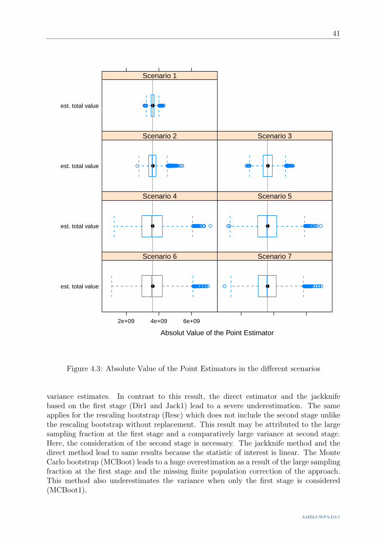
41

Absolut Value of the Point Estimator

est. total value

2e+09 4e+09 6e+09

● ●●● ●●●●●● ● ●●● ● ●●●● ●● ●●●●●● ●●● ●●●● ●●● ●●●●●

Scenario 6

●● ●●● ● ●●● ●● ●●● ●●●●● ●●●● ●●● ●● ●●●● ●●● ●● ●●● ●●●●●●● ●●● ●●

Scenario 7

est. total value ● ● ●●●●●●●●●● ●● ●●●●●●●●●●●●●●● ●●●●●● ●●●●● ●●

Scenario 4

● ●●●●● ●●●●●●● ●●●● ●●●● ● ●●●●●●●●●●●●● ●●●●●● ●●● ●●●● ●

Scenario 5

est. total value ●●●●●●●●● ●●● ●●●● ●● ● ●●●●●●●●●●●●●●●● ●●● ●●●●●●●●●●●●●●●●●● ●●●●●●●●●●● ●● ●●●● ●● ●●●●●●●● ●●●●●●●●●●● ●● ●● ●●●●●●● ●● ●●●●●● ●●●●●●●● ●●●●●●●●●● ●●●●●●●●●●●● ● ●●

Scenario 2

●●● ●●●● ●●● ●●●●● ●●●●●●●●●●●●●● ●●●●● ●●●●●●● ●●● ●●● ●● ●●●● ●●●● ●●●●● ●●●●●●●

Scenario 3

est. total value ●●●●●●●●●● ●●●●●● ●●●●●●●●●●● ●●●●●●●●●●●● ●●●●●●●●● ●●●●●● ●●● ●●●●● ●●●●● ●●● ●● ●●● ●●● ●●●

Scenario 1

Figure 4.3: Absolute Value of the Point Estimators in the different scenarios

variance estimates. In contrast to this result, the direct estimator and the jackknifebased on the first stage (Dir1 and Jack1) lead to a severe underestimation. The sameapplies for the rescaling bootstrap (Resc) which does not include the second stage unlikethe rescaling bootstrap without replacement. This result may be attributed to the largesampling fraction at the first stage and a comparatively large variance at second stage.Here, the consideration of the second stage is necessary. The jackknife method and thedirect method lead to same results because the statistic of interest is linear. The MonteCarlo bootstrap (MCBoot) leads to a huge overestimation as a result of the large samplingfraction at the first stage and the missing finite population correction of the approach.This method also underestimates the variance when only the first stage is considered(MCBoot1).

AMELI-WP3-D3.1


Absolute Value of the Variance Estimation

DirDir1Jack

Jack1MCBoot

MCBoot1Resc

RescWoR

5.0e+17 1.5e+18 2.5e+18

●●●●● ●●●● ●●

●●●●● ●●●● ●●

●●●●● ●●●● ●●

●●●●● ●●●● ●●

● ●●●● ●●●●● ●●● ●●●

● ●●● ●●●●● ●●● ●●●

● ●●● ●●● ●●●●● ●● ●●● ●●

●● ●●●● ●●●●● ●● ●●

●

●

●

●

●

●

●

●

Scenario 6

●● ●●● ●● ●● ●● ●●●●● ●●● ●● ●●● ●● ● ●●● ●●●● ●

●● ●●● ●● ●● ●● ●●●●●● ●●● ●● ●●●●● ● ●● ●●●●

●● ●●● ●● ●● ●● ●●●●● ●●● ●● ●●● ●● ● ●●● ●●●● ●

●● ●●● ●● ●● ●● ●●●●●● ●●● ●● ●●●●● ● ●● ●●●●

●● ●●●● ●●● ●● ●●● ●● ●● ●●●● ●●● ●●●●● ●●● ●● ●●● ●●●● ●● ●●● ●

●● ●●●● ●● ● ●●● ●●● ●●●●●●● ●●●●● ●●● ●● ●● ●● ●●●●●

●● ●● ●● ●● ●● ●●● ●● ●●● ●●●●●● ●● ●●● ●●● ●●●● ● ● ●●●● ●● ●●●

●● ●●● ●● ●●● ●● ●●● ● ●●● ●● ● ●●●●● ●● ●●● ●●● ●● ●●●●● ●

●

●

●

●

●

●

●

●

Scenario 7Dir

Dir1Jack

Jack1MCBoot

MCBoot1Resc

RescWoR

●●● ●●●● ●

●●● ●●● ●

●●● ●●●● ●

●●● ●●● ●

●●●●●●●● ●●● ●● ●●●

●●●●●●●● ●●● ●● ●●●

●●●●● ●● ● ●●●

●●●●●●

●

●

●

●

●

●

●

●

Scenario 4

●●●●●●●●●●● ●● ● ●●●●● ●●

●●●●●●●●● ●● ●●●●● ●●

●●●●●●●●●●● ●● ● ●●●●● ●●

●●●●●●●●● ●● ●●●●● ●●

●●●●●● ●●●●●●●● ● ●●● ●● ●● ●●●● ●●● ●●● ●●●●

●●●●●● ●●●●●●●● ● ●●● ●● ●● ●●●● ●●● ●●● ●●●●

●●● ●●●●●●●●● ●● ●●● ●●●● ●●●●● ●● ●●●●●

●●● ●●● ●●●●●●● ●●●●●● ● ●●●

●

●

●

●

●

●

●

●

Scenario 5Dir

Dir1Jack

Jack1MCBoot

MCBoot1Resc

RescWoR

●●●●● ●●●●● ●●● ●● ● ●●● ●●● ●●● ● ●● ●● ●● ●● ●● ●●●●●● ●●●● ●●●● ●● ●●● ●●●● ● ●●●●●● ●●● ●●● ●●● ●●●●●●● ●●● ●●●●●● ●●●●● ●●●●● ●●● ●● ●●● ● ●●● ● ●●●● ●●● ●●● ● ●● ●●● ● ●●●●● ●● ●●●●●● ● ●●● ●●● ●● ●●● ●●●● ●● ● ●●●● ●●● ●●●●● ●●●●●● ●●●●● ●● ●●●●● ●●●● ● ●● ●●● ●● ● ●●●● ● ●●●● ●●●●●●●● ● ● ●● ●●● ●●●●●●●● ●● ● ●● ●●●●● ●● ●●●● ●●●● ●● ●●●● ● ●●●●●●●● ●● ●●●●●●●●●●●●● ● ●● ●●● ●● ●● ●● ●● ●●● ● ●● ● ●●●●● ●●● ●●●● ●●● ●● ●●●●●● ●●●●●● ●●● ●● ● ●●●●● ●● ●● ●●●●●● ● ●●● ●●●●● ●●●● ●●● ●● ●●●●●●●●●● ●● ●● ● ●●●● ● ●●●●● ●●●● ●●●●●●●● ● ●●● ●●●● ●●● ●●● ●● ● ● ●● ●●●●● ●●●●● ●●● ●●●● ● ●● ●●● ●● ●●●●● ●●●● ●● ●●●● ●●●● ●● ●●● ●● ●● ●●● ●●● ●●●●● ●●● ●●●● ●●●●●●●● ●●●● ● ●● ●● ●● ●●● ●●● ●●● ●●●● ● ●●● ●●● ● ●●● ●●● ●●●●●●●● ●●● ●● ●● ●● ●●● ●●● ●●●● ●● ●● ●●●● ●●●● ●●● ●●●●●● ●● ●●●● ● ●●●● ●● ● ●● ● ●● ●●●●● ●●●● ●● ●●● ●●●● ●●●●● ●●●● ●●●●●● ●● ●●●● ● ●●● ●●●● ●●● ●●● ●●●●● ●●●●● ●●● ●●●●● ●●●●●●● ●●●● ●●●● ●● ● ●●● ●●● ●●● ●●●●●●● ●● ● ● ●●●●●●●● ●●●● ●● ●●● ●●● ●●●● ● ●●● ●● ●●● ●● ●● ●● ●

●● ●●● ●●●●● ●●● ●● ●●●●● ●●● ●● ●●● ●● ●● ●●●●●●● ●●●● ●●●● ●● ●● ●●●● ● ●●●●●● ●●● ●●●●●● ●●●●● ●● ●●●●●●●●● ●●●●●● ●●●●● ●●●●● ●●● ● ●●● ● ●●●●●● ●●●● ●●●● ● ●●●●● ●●● ●●●●●● ● ●●● ●●● ●● ●●● ●●●● ●● ●● ●●● ●●● ●●●●● ●●●●●● ●●●●● ●● ●●●● ●●●● ●●● ●●● ●●● ●●●● ● ●●●● ●●●●●●● ● ●● ●●● ●●●●●●●● ●● ● ●● ●●●●●● ●● ●●●● ●● ●● ●● ●●●● ● ●●●●●●●●●● ●●●●●●●●●●● ●● ●●● ●● ●●● ●● ●●● ● ●●● ●●●●● ●●●● ●●● ●● ●● ●●●●●● ●●●●●● ●●● ●● ●●●●●● ●●●●●●●● ●●●● ●●●● ● ●●●●●● ●●● ●●●●●●●●●● ●● ●● ● ●●●● ● ●●●●● ●●●● ●●●●●● ● ●●●● ●●● ●●● ●● ●● ● ●● ●●● ●●● ●●●● ●●● ●●●● ●●● ●●● ●● ●●●●● ●●●● ●● ●●●● ●●●● ●● ●●● ●●● ●●●●●● ●●●●● ●●●●●● ●●●●●● ●●●●● ● ●● ●● ●● ●●● ●●● ●●● ●●● ● ●●●● ●●●● ●●● ●●● ●●●●●●● ●●● ●● ●● ●● ●●● ●●●●●●● ●● ●● ●●●● ●●●● ●●● ●●●●●●● ●● ●●●● ● ●● ●● ● ●● ● ●● ●●●●●● ●●● ●● ●● ●●● ●●●● ●●●●● ●●●●● ●● ●●●● ●● ●●●● ● ●●● ●●●●● ●●● ●●● ●●●●● ●●●● ●●● ●●●● ●●●● ●●● ●●●● ●●●● ●●● ●●● ●● ●●● ●●●●●● ●●● ● ●●●●●● ●●●●●●● ●● ●●● ●●● ●●●● ● ●●●● ●●● ●●● ●● ●●

●●●●● ●●●●● ●●● ●● ● ●●● ●●● ●●● ● ●● ●● ●● ●● ●● ●●●●●● ●●●● ●●●● ●● ●●● ●●●● ● ●●●●●● ●●● ●●● ●●● ●●●●●●● ●●● ●●●●●● ●●●●● ●●●●● ●●● ●● ●●● ● ●●● ● ●●●● ●●● ●●● ● ●● ●●● ● ●●●●● ●● ●●●●●● ● ●●● ●●● ●● ●●● ●●●● ●● ● ●●●● ●●● ●●●●● ●●●●●● ●●●●● ●● ●●●●● ●●●● ● ●● ●●● ●● ● ●●●● ● ●●●● ●●●●●●●● ● ● ●● ●●● ●●●●●●●● ●● ● ●● ●●●●● ●● ●●●● ●●●● ●● ●●●● ● ●●●●●●●● ●● ●●●●●●●●●●●●● ● ●● ●●● ●● ●● ●● ●● ●●● ● ●● ● ●●●●● ●●● ●●●● ●●● ●● ●●●●●● ●●●●●● ●●● ●● ● ●●●●● ●● ●● ●●●●●● ● ●●● ●●●●● ●●●● ●●● ●● ●●●●●●●●●● ●● ●● ● ●●●● ● ●●●●● ●●●● ●●●●●●●● ● ●●● ●●●● ●●● ●●● ●● ● ● ●● ●●●●● ●●●●● ●●● ●●●● ● ●● ●●● ●● ●●●●● ●●●● ●● ●●●● ●●●● ●● ●●● ●● ●● ●●● ●●● ●●●●● ●●● ●●●● ●●●●●●●● ●●●● ● ●● ●● ●● ●●● ●●● ●●● ●●●● ● ●●● ●●● ● ●●● ●●● ●●●●●●●● ●●● ●● ●● ●● ●●● ●●● ●●●● ●● ●● ●●●● ●●●● ●●● ●●●●●● ●● ●●●● ● ●●●● ●● ● ●● ● ●● ●●●●● ●●●● ●● ●●● ●●●● ●●●●● ●●●● ●●●●●● ●● ●●●● ● ●●● ●●●● ●●● ●●● ●●●●● ●●●●● ●●● ●●●●● ●●●●●●● ●●●● ●●●● ●● ● ●●● ●●● ●●● ●●●●●●● ●● ● ● ●●●●●●●● ●●●● ●● ●●● ●●● ●●●● ● ●●● ●● ●●● ●● ●● ●● ●

●● ●●● ●●●●● ●●● ●● ●●●●● ●●● ●● ●●● ●● ●● ●●●●●●● ●●●● ●●●● ●● ●● ●●●● ● ●●●●●● ●●● ●●●●●● ●●●●● ●● ●●●●●●●●● ●●●●●● ●●●●● ●●●●● ●●● ● ●●● ● ●●●●●● ●●●● ●●●● ● ●●●●● ●●● ●●●●●● ● ●●● ●●● ●● ●●● ●●●● ●● ●● ●●● ●●● ●●●●● ●●●●●● ●●●●● ●● ●●●● ●●●● ●●● ●●● ●●● ●●●● ● ●●●● ●●●●●●● ● ●● ●●● ●●●●●●●● ●● ● ●● ●●●●●● ●● ●●●● ●● ●● ●● ●●●● ● ●●●●●●●●●● ●●●●●●●●●●● ●● ●●● ●● ●●● ●● ●●● ● ●●● ●●●●● ●●●● ●●● ●● ●● ●●●●●● ●●●●●● ●●● ●● ●●●●●● ●●●●●●●● ●●●● ●●●● ● ●●●●●● ●●● ●●●●●●●●●● ●● ●● ● ●●●● ● ●●●●● ●●●● ●●●●●● ● ●●●● ●●● ●●● ●● ●● ● ●● ●●● ●●● ●●●● ●●● ●●●● ●●● ●●● ●● ●●●●● ●●●● ●● ●●●● ●●●● ●● ●●● ●●● ●●●●●● ●●●●● ●●●●●● ●●●●●● ●●●●● ● ●● ●● ●● ●●● ●●● ●●● ●●● ● ●●●● ●●●● ●●● ●●● ●●●●●●● ●●● ●● ●● ●● ●●● ●●●●●●● ●● ●● ●●●● ●●●● ●●● ●●●●●●● ●● ●●●● ● ●● ●● ● ●● ● ●● ●●●●●● ●●● ●● ●● ●●● ●●●● ●●●●● ●●●●● ●● ●●●● ●● ●●●● ● ●●● ●●●●● ●●● ●●● ●●●●● ●●●● ●●● ●●●● ●●●● ●●● ●●●● ●●●● ●●● ●●● ●● ●●● ●●●●●● ●●● ● ●●●●●● ●●●●●●● ●● ●●● ●●● ●●●● ● ●●●● ●●● ●●● ●● ●●

●●● ●●● ●●●●●●●●● ●● ●●● ●●● ●● ● ●● ●● ●● ●● ●● ●● ●●●●● ●●●● ●●●●● ●● ● ●●● ●●●● ●●● ●●● ●●● ●●● ●●●● ● ● ●● ● ●●●●●● ●●●●●● ●●●●● ●●● ●● ●● ● ● ●● ●● ● ●●●● ●● ● ●●● ● ●●●●● ●●● ●●● ●●● ●●● ●●● ● ●●● ●●● ●● ●● ●●●● ●● ● ●●●● ●●● ●● ●●●● ●●●●●● ●●●●●● ●●● ●●● ●●●● ● ●● ●●● ●● ● ●●●● ● ●●●●● ●● ●●●●● ● ● ●● ●●● ●●●●● ●●● ●● ● ●● ●●● ●● ● ●● ●●●● ● ●●●● ●● ●●●●● ● ●●●●●●●●● ●● ●●●●●●●●● ● ● ● ●● ●●● ●● ●●● ●● ●● ●● ● ●● ● ●●●●● ●●● ●●●● ●●● ●● ●●●● ●● ●●●●●● ●●● ●● ●●●●●●● ●● ●● ●●●●●● ● ●●● ●●●●● ●●● ●● ●●● ●●● ●●●●●●●●●●● ●● ●● ● ●●●● ● ●●● ●●● ●●●● ●●●●●●● ● ●●●● ●●● ●●● ●●● ●●● ● ● ●● ●● ●●● ●●●● ●●● ●●●● ● ●● ●● ● ●● ●●●●● ●●●● ●● ●●●● ●●●● ●● ●●●● ●●● ●● ●●● ● ●●● ●● ●●● ●●●● ●●●●●●●●● ●● ●●● ● ● ●● ●●● ●●● ● ●● ●●●●●● ● ●●● ●●● ● ●●● ●●●● ●●●●●●● ●●● ●● ●● ●● ●●● ● ●● ●●●● ●● ●● ●●●● ●●●● ●●● ●● ●●● ●● ●● ●●●●● ● ●●● ●● ● ●● ● ●● ●●●●● ●●●● ●● ●●● ●●●● ●●● ●● ●●●● ●●●●●● ●● ●●●● ● ●●● ●●●● ●●● ●●● ●●●●● ●●●● ●●● ●●●● ●● ●● ●●● ● ●● ● ●●●●● ●● ● ●●●●● ● ●●● ●●●●●● ●● ● ●●●●●●●●●●●●● ●● ●●● ●●●●●● ●●●● ●● ●●● ●● ●●● ●● ●

●●● ●●● ●●●●●●●●● ●● ●●● ●● ●● ●● ● ●● ●●● ●● ●● ●●●●●●●● ●●●● ●●●●● ●● ● ●●● ●●●●●●● ●●●●●●●● ●●● ● ● ●● ●●●●●●● ●●●●●● ●●●● ●● ●●●●● ●● ● ● ●●● ● ●●●● ●● ●●● ●●●●● ●●● ●●● ●●● ●●● ●●● ● ●● ●●● ●● ●● ●●●● ●● ●● ●●● ●●● ●● ●●●● ● ●●●●● ●●●●●● ●● ●●● ●●●● ●●● ●●● ●● ● ●●●●● ● ●●●●● ●●● ●●●● ● ●● ●●● ●●●●● ●●● ●● ● ●● ●●●●● ● ●● ●●●● ●● ●●● ●● ●●●● ● ●● ●●●● ●●●● ●● ●●●●●●●●●● ●● ●● ●●● ●● ●●●● ●● ● ●● ● ●● ● ●●●●● ●●● ●●● ●●● ●● ●●●●●● ●●●●● ●●● ●● ●●●●●●● ● ●●●● ●●● ● ●●● ●●●● ● ●● ●● ●●● ●●● ●●●● ●●●●●●● ●● ●● ● ●●●● ● ●●● ●●● ●●●● ●●●●●● ● ●●●● ●●● ●●● ●●● ●● ● ● ●● ●● ●●● ●●●● ●●● ●●●● ● ●● ●●● ●● ●●●●● ●●●● ●● ●●● ●●●● ●● ●●●● ●●● ●● ●●● ● ●●● ● ●●●●●●● ●●●●●●●● ●● ●●● ● ● ●● ●●● ●● ●●● ●●●●●● ● ●●● ●●● ● ●●● ●●●● ●●●●● ● ●●● ●● ●● ●● ●●● ● ●● ●●●● ●● ●● ●●●● ●●●● ●●● ●● ●●● ●● ●● ●●●●● ● ●●● ●● ● ●● ● ●● ●●●●● ●●●● ●● ● ●●● ●●● ●●● ●● ●● ●● ●● ●●●● ●● ●●●● ● ●●● ●●●●● ●●● ●●● ●●●●● ●●●●●●● ●●●● ●● ●● ●●● ●● ●● ●●●●● ●● ● ● ●●●● ● ●● ●●●●●● ●● ● ● ●●●●●●●●●●●● ●● ●●● ●●●●●● ●●●●● ●●● ●● ●●● ●● ●

●● ●●●●●●●●●●● ●● ●●● ●● ●●● ●● ●●● ●● ●● ●●●●●●●● ●●●● ● ●●● ●● ●● ● ●●● ●●●●●● ●●●●●●●●● ●●●● ● ●●●● ●●●●●● ●●●● ●●●● ● ●●●●● ●●● ● ●●● ● ●●●●●●● ●●●● ●●●● ●●●●●● ●●● ●●●●●● ● ●●● ●●●● ●● ●● ●●●●● ●●● ●●●● ●●● ●●●●● ●●●●●● ●●●●●●● ●● ●●●● ●●●● ● ●●●●● ●●●●● ●● ●●●●● ●●●●●●●● ●●● ●●● ●●●●●●●● ●● ● ●● ●●●●●● ●● ●●●● ●●●● ●● ●●● ● ●●●●●●●●● ●●● ●●●●●●●●●●●●●● ●● ●●● ●● ●●●● ●● ●●● ● ●●● ●●●●●● ●●●● ●●● ●● ●● ● ●●●●● ●●●● ●●●● ●●● ●●●● ●●●●●● ●● ●●●●●●●●●● ●●●● ● ●●● ●●● ●●● ●●●●●●●●●● ●● ●● ● ●●● ● ●●● ●●● ●●●● ●●●●●●●● ● ●●●●●●● ●●● ●●● ●● ● ● ●●●●● ●●●● ●●●●● ●●● ●●●● ●● ●● ●●● ●●● ●●●●● ●●●● ● ●●●●●● ●● ●●● ●●● ●●●● ●●●●● ●●●●●● ●● ●● ●●●●● ●● ●●●● ● ●● ●● ●●● ●●● ●●● ●●●●●● ● ●●●● ●●●● ●● ●●●● ●●●●● ●●● ●● ●● ●● ●●●●●●●●● ●● ●● ●● ● ●●●● ●●● ●●●●●●● ●● ●●●● ●●●● ●● ● ●● ● ●● ●●●●● ●●● ●● ●●● ●●●● ●●●● ●●●●● ●●●●●● ●● ●●●● ● ●●● ●●●●● ●●● ●●● ●●●●● ●●●●●●● ●●●● ●● ●● ●●●●●●● ●●●● ●● ● ●●● ●● ●●●●●●●●●● ●●● ●● ●●●●● ●●●●●●● ●● ●● ●●● ●●●● ●●●●●● ●●● ●● ●● ●●

●●●● ●●●●●● ●●● ●● ● ●●● ●● ●● ●● ●● ●● ● ●● ●● ●●●●●●●● ●●●● ●●●●● ●● ●●●● ● ●●●●●● ●●● ●●● ●●● ●●●●● ●● ●●● ●●●●●● ●●●● ●●●● ● ●●● ●● ●●● ● ●● ●● ● ●●●● ●● ●●●● ●● ●●● ● ●●●●●●●● ●●●●●● ● ●●● ●● ●● ●●● ●●●● ●● ● ●●●● ●●●● ●●●●● ●●●●●● ●●●●●● ●● ●●●●● ●●●●● ●● ●●● ●● ● ●● ●●● ● ●●●● ●●●●●●●● ● ● ●● ●●● ●●●●●●●●● ●●● ●● ●●●●● ● ●● ●●● ●● ●●●● ●● ●●●● ● ●●●●● ●●● ●●●● ●●●●●●●●●●●● ●●● ●●● ●●● ●●● ●● ●●● ●● ● ●● ●● ●●●●● ●●● ●●●● ●● ●● ●●●●●● ●●●●●● ●●● ●● ● ●●●●● ● ●● ●●●● ●● ●● ● ●●● ●●●●● ●●●● ●●● ●● ●●●●●●●●●●● ●● ●● ● ●●●● ● ●●●●● ●●●● ●●●●●● ● ●●● ●●●● ●●● ●● ●● ● ● ●● ●●● ●●● ●●●●● ●●● ●●●● ● ●● ●●● ●● ●●●●● ●●●● ●● ●●●● ●●●● ●● ●●●● ●●●● ●●● ●●● ●●●●● ●●● ●●●● ●●●●●●●● ●●●●● ● ●● ●● ●●● ●●● ●● ●● ●●●●●●● ● ●●● ●●● ● ●●● ●●●● ●●●●●●● ●●●● ●● ●●● ●● ●●● ●●● ●●●●● ●● ●● ●●●●● ●●●● ●●● ●●●●●●● ●● ●●●● ●●●● ●● ● ● ●● ● ●● ●●●● ●●●● ●● ●●● ●●●● ●●●●● ●●●● ●●●●●● ●● ●● ●●● ● ●●● ●●●● ●●● ●●● ●●●●● ●●●● ●●● ●●●●● ●● ●●●●●● ●●●● ●●●● ●● ● ● ●●●●● ● ●● ●●●●●●● ●● ● ● ●●●●● ●●●●●● ●● ●●● ● ●●●●●● ● ●●●● ●●● ●● ●● ●●

●

●

●

●

●

●

●

●

Scenario 2

●●●●●●●●●●●●●●●● ●●●●●●●●●●●●●●●●●●●●●●●●●●● ●●●●● ●●●● ●●●●●●●●●●●●●●●●● ●●●●●●●●●●●●●●●●●●●●●●●●●●●●●●●●●●●●●●●●●●●●●●●●●● ●● ●●●●● ●● ●●●●● ●●● ●●●●●●●● ●●●●● ●●●●●●●●●●●●●●●●●●●●●●●●●●●●●●●●●●●●●●

●●●●●●●●●●●●●●● ●●●●●●●●●●●●●●●●●●●●●●●●●●● ●●●● ●●●● ●●●●●●●●●●●●●●●● ●●●●●●●●●●●●●●●●●●● ●●●●●●●●●●●●●●●●●●●●●●●●●●●●●●●●● ●● ●●● ●● ●●●●● ●●●● ●●●●●●●● ●●●●● ●●●●●●●●●●●●●●●●●●●●●●●●●●●●●●●●●●●●●●●

●●●●●●●●●●●●●●●● ●●●●●●●●●●●●●●●●●●●●●●●●●●● ●●●●● ●●●● ●●●●●●●●●●●●●●●●● ●●●●●●●●●●●●●●●●●●●●●●●●●●●●●●●●●●●●●●●●●●●●●●●●●● ●● ●●●●● ●● ●●●●● ●●● ●●●●●●●● ●●●●● ●●●●●●●●●●●●●●●●●●●●●●●●●●●●●●●●●●●●●●

●●●●●●●●●●●●●●● ●●●●●●●●●●●●●●●●●●●●●●●●●●● ●●●● ●●●● ●●●●●●●●●●●●●●●● ●●●●●●●●●●●●●●●●●●● ●●●●●●●●●●●●●●●●●●●●●●●●●●●●●●●●● ●● ●●● ●● ●●●●● ●●●● ●●●●●●●● ●●●●● ●●●●●●●●●●●●●●●●●●●●●●●●●●●●●●●●●●●●●●●

●●●●●●●●●●●●●● ●●●●●●●●●●●● ●●●●●●●●●●●●● ●●● ●●●● ●●●●●●●●●●● ●●●●●●●●●●●●●●●● ●●● ●●●●●● ●●●●●●●●●●●●●●●●●●●●●●●●● ●●● ●●●●● ●●●●● ●● ●● ●●●●● ●●●●●●●●●● ●●● ●●●●●● ●●●●●●●●●●●●●●●●●●●●●●● ●●●●●●●●●●●● ●●●● ●

●●●●●● ●●●●●●●● ●●●●●●●●●●●●● ●●●●●●●●●●●●● ●●● ●●●● ●●●●●●●●●● ●●●●●●●●●●●●●●● ●●● ●●●●●● ●●●●●●●●●●●●●●●●●●●●●●●●● ●●●●●●● ●●●●● ●● ●● ●●●●● ●●●●●●●●●● ●●● ●●●●●● ●●●●●●●●●●●●●●●●●●●●●●● ●●●●●●●●●●●● ●●●● ●

●●●●●●●●●●●●●● ●●●●●●●●●●●●●●●●●●●●●●●●●●●●●●●● ●●●●●●●●● ●●●●●●●●●●●●●●●●●●●●●●●●●●●●●●●●●●●●●●●●●●●●●●●●●●●●●●●●● ●●●●●● ●●●●●●●●●●●●● ●● ●●● ●● ●●●●●●●●●●●●●●●●● ●●●● ●●●●●●●●●●●●●●●●●●●●●●●●●●●●●●●●●●●●●●●●●

●●●●●●●●●● ●●●●●●●●● ●●●●●●●●●●●●●●●●●●●●●●●●●●●● ●●●●●●●●● ●●●●●●●●●●●●●●● ●●●●●●●●●●●●●●●●●● ●●●●●● ●●● ●●●●●●●●●●●●●● ●●●●●●●● ●● ●●●● ●●● ●●●●● ●●●● ●●●●●●● ●●● ●●●●● ●●●●●●●●●●●●●●●●●●●●● ●●●●●●●●●●●●●●●●

●

●

●

●

●

●

●

●

Scenario 3Dir

Dir1Jack

Jack1MCBoot

MCBoot1Resc

RescWoR

●●●●●●●●●●●●●●●●●●●●●●●●●●●●●●●●●●●●●●●●●●●●●●●●●●●●●●●●●●●●●●●●●●●●●●●●●●●●●●●●●●●●●●●●●●●●●●●●●●●●●●●●●●●●●●●●●●●●●●●●●●●●●●●●●●●●●●●●●●●●●●●●●●●●●●●●●●●●●●●●●●●●●●●●●●●●●●●●●●●●●●●●●●●●●●●●●●●●●●●●●●●●●●●●●●●●●●●●●●●●●●●●●●●●●●●●●●●●●●●●●●●●●●●●●●●●●●●●●●●●●●●●●●●●●●●●●●●●

●●●●●●●●●●●●●●●●●●●●●●●●●●●●●●●●●●●●●●●●●●●●●●●●●●●●●●●●●●●●●●●●●●●●●●●●●●●●●●●●●●●●●●●●●●●●●●●●●●●●●●●●●●●●●●●●●●●●●●●●●●●●●●●●●●●●●●●●●●●●●●●●●●●●●●●●●●●●●●●●●●●●●●●●●●●●●●●●●●●●●●●●●●●●●●●●●●●●●●●●●●●●●●●●●●●●●●●●●●●●●●●●●●●●●●●●●●●●●●●●●●●●●●●●●●●●●●●●●●●●●●●●●●●●●●●●●

●●●●●●●●●●●●●●●●●●●●●●●●●●●●●●●●●●●●●●●●●●●●●●●●●●●●●●●●●●●●●●●●●●●●●●●●●●●●●●●●●●●●●●●●●●●●●●●●●●●●●●●●●●●●●●●●●●●●●●●●●●●●●●●●●●●●●●●●●●●●●●●●●●●●●●●●●●●●●●●●●●●●●●●●●●●●●●●●●●●●●●●●●●●●●●●●●●●●●●●●●●●●●●●●●●●●●●●●●●●●●●●●●●●●●●●●●●●●●●●●●●●●●●●●●●●●●●●●●●●●●●●●●●●●●●●●●●●●

●●●●●●●●●●●●●●●●●●●●●●●●●●●●●●●●●●●●●●●●●●●●●●●●●●●●●●●●●●●●●●●●●●●●●●●●●●●●●●●●●●●●●●●●●●●●●●●●●●●●●●●●●●●●●●●●●●●●●●●●●●●●●●●●●●●●●●●●●●●●●●●●●●●●●●●●●●●●●●●●●●●●●●●●●●●●●●●●●●●●●●●●●●●●●●●●●●●●●●●●●●●●●●●●●●●●●●●●●●●●●●●●●●●●●●●●●●●●●●●●●●●●●●●●●●●●●●●●●●●●●●●●●●●●●●●●●

●●●●●●●●●●●●●●●●●●●●●●●●●●●●●●●●●●●●●●●●●●●●●●●●●●●●●●●●●●●●●●●●●●●●●●●●●●●●●●●●●●●●●●●●●●●●●●●●●●●●●●●●●●●●●●●●●●●●●●●●●●●●●●●●●●●●●●●●●●●●●●●●●●●●●●●●●●●●●●●●●●●●●●●●●●●●●●●●●●●●●●●●●●●●●●●●●●●●●●●●●●●●●●●●●●●●●●●●●●●●●●●●●●●●●●●●●●●●●●●●●●●●●●●●●●●●●●●●●●●●●●●●●●●●●●●●●●●●●●●●●●●●●●●●●●●

●●●●●●●●●●●●●●●●●●●●●●●●●●●●●●●●●●●●●●●●●●●●●●●●●●●●●●●●●●●●●●●●●●●●●●●●●●●●●●●●●●●●●●●●●●●●●●●●●●●●●●●●●●●●●●●●●●●●●●●●●●●●●●●●●●●●●●●●●●●●●●●●●●●●●●●●●●●●●●●●●●●●●●●●●●●●●●●●●●●●●●●●●●●●●●●●●●●●●●●●●●●●●●●●●●●●●●●●●●●●●●●●●●●●●●●●●●●●●●●●●●●●●●●●●●●●●●●●●●●●●●●●●●●●●●●●●●●●●●●●●●●●●●

●●●●●●●●●●●●●●●●●●●●●●●●●●●●●●●●●●●●●●●●●●●●●●●●●●●●●●●●●●●●●●●●●●●●●●●●●●●●●●●●●●●●●●●●●●●●●●●●●●●●●●●●●●●●●●●●●●●●●●●●●●●●●●●●●●●●●●●●●●●●●●●●●●●●●●●●●●●●●●●●●●●●●●●●●●●●●●●●●●●●●●●●●●●●●●●●●●●●●●●●●●●●●●●●●●●●●●●●●●●●●●●●●●●●●●●●●●●●●●●●●●●●●●●●●●●●●●●●●●●●●●●●●●●●●●●●●●

●●●●●●●●●●●●●●●●●●●●●●●●●●●●●●●●●●●●●●●●●●●●●●●●●●●●●●●●●●●●●●●●●●●●●●●●●●●●●●●●●●●●●●●●●●●●●●●●●●●●●●●●●●●●●●●●●●●●●●●●●●●●●●●●●●●●●●●●●●●●●●●●●●●●●●●●●●●●●●●●●●●●●●●●●●●●●●●●●●●●●●●●●●●●●●●●●●●●●●●●●●●●●●●●●●●●●●●●●●●●●●●●●●●●●●●●●●●●●●●●●●●●●●●●●●●●●●●●●●●●●●●●●●●●●●●●●●●●●●●●●●●●●●●●●●●●●●●

●

●

●

●

●

●

●

●

Scenario 1

Figure 4.4: Absolute Value of the Variance Estimation Methods in the different scenarios

In scenario 2, the variance within the different PSUs is unequal. Due to high variances insome PSUs (cf. 4.1) the variance at the second stage increases as opposed to scenario 1.For that reason the methods without considering the second stage also show a significantunderestimation. But due to the generation process also the variability of the mean of thePSUs rises and with that the variance at first stage opposite scenario 1. Thus, the relativebias of these methods is smaller than in this situation. The methods which consider thesecond stage lead to unbiased estimates. These methods yield, however, also a lot ofoutliers through the high variance within some PSUs.

A converse effect appears when only the expected value between the PSUs varies. Hence,in scenario 3, there is only a small difference between the methods which include allstages and the methods which only consider the first stage. This is a result of the varying



43

Absolute Value of the Variance Estimation

DirDir1Jack

Jack1MCBoot

MCBoot1Resc

RescWoR

0 2 4 6

●●●●●●●●● ●●

●●●●●●●●● ●●

●●●●●●●●● ●●

●●●●●●●●● ●●

● ●●●● ●●●●● ●●● ●●●

● ●●● ●●●●● ●●● ●●●

● ●●●●●● ●●●●●●●●●● ●●

●●●●●● ●●●●●●● ●●

●

●

●

●

●

●

●

●

Scenario 6

●● ●●● ●● ●● ●● ●●●●● ●●●●● ●●●●● ● ●●● ●●●● ●

●● ●●● ●● ●● ●● ●●●●●● ●●●●● ●●●●● ● ●● ●●●●

●● ●●● ●● ●● ●● ●●●●● ●●●●● ●●●●● ● ●●● ●●●● ●

●● ●●● ●● ●● ●● ●●●●●● ●●●●● ●●●●● ● ●● ●●●●

●● ●●●● ●●● ●● ●●● ●● ● ●● ●●●●●●● ●●●●● ●●● ●● ●●● ●●●● ●● ●●● ●

●● ●●●● ●● ●●●● ●● ●● ●●●●●●● ●●●●● ●●● ●● ●● ●● ●●●●●

●● ●● ●● ●● ●● ●●●●● ●●● ●●●●●● ●●●●● ●●●●●●●● ● ●●●● ●●●●●

●● ●●● ●● ●●● ●● ●●●● ●●● ●● ●●●●●● ●●●●● ●●● ●● ●●●●● ●

●

●

●

●

●

●

●

●

Scenario 7Dir

Dir1Jack

Jack1MCBoot

MCBoot1Resc

RescWoR

●●●●●●●●

●●●●●●●

●●●●●●●●

●●●●●●●

●●●●●●●● ●●●●●●●●

●●●●●●●● ●●●●●●●●

●●●●●●●●●●●

●●●●●●

●

●

●

●

●

●

●

●

Scenario 4

●●●●●●●●●●●●●●●●●●● ●●

●●●●●●●●●●●●●●●● ●●

●●●●●●●●●●●●●●●●●●● ●●

●●●●●●●●●●●●●●●● ●●

●●●●●● ●●●●●●●●●●●●●●●● ●●●● ●●● ●●● ●●●●

●●●●●● ●●●●●●●●●●●●●●●● ●●●● ●●● ●●● ●●●●

●●● ●●●●●●●●●●●●●● ●●●● ●●●●● ●● ●●●●●

●●●●●●●●●●●●●●●●●●●● ●●●

●

●

●

●

●

●

●

●

Scenario 5Dir

Dir1Jack

Jack1MCBoot

MCBoot1Resc

RescWoR

●● ●●● ●●●● ● ●●● ●● ● ●●● ● ●● ●●● ● ●● ●● ●● ●● ●● ●●●●●● ●●●● ● ●●● ●● ●●● ●●●● ● ●●● ●●● ● ●● ●●● ●●● ●●● ● ● ●● ●● ● ●●●●●● ●●●● ● ●●●● ● ●●● ●● ●● ● ● ●●● ● ●●●● ●● ● ●●● ● ●● ●●● ● ● ●●● ● ●● ●● ●●●● ● ●●● ●●● ●● ●● ● ●●●● ●● ● ●●●● ●●● ●●●●● ● ● ●●●● ●●● ●● ●● ●●●●● ●●●● ● ●● ●●● ●● ● ●●●● ● ●●● ● ●●●●●●● ● ● ● ●● ●●● ●●●●● ●●● ●● ● ●● ●●●● ● ●● ●●●● ● ●●● ●● ●● ●● ● ●●●●● ● ●● ●● ●●●●●● ●●●●● ● ● ● ●● ●●● ●● ●● ●● ●● ●●● ● ●● ● ●●● ●● ●●● ●●●● ●●● ●● ● ●●● ●● ●●●●●● ●●● ●● ● ●● ●● ● ●● ●● ●●●●●● ● ●●● ●●●●● ● ●●● ●●● ●● ● ●●●●●●● ●● ●● ●● ● ●●● ● ● ●●●●● ●●●● ●●● ●●● ●● ● ●●● ● ●● ● ●●● ●●● ●● ● ● ●● ●●●●● ●● ●●● ●●● ●●●● ● ●● ●● ● ●● ●●● ●● ●●●● ●● ●●●● ●●●● ●● ●●● ●● ●● ●●● ●●● ●●● ●● ●●● ●● ●● ●● ●●●●●● ●●● ● ● ●● ●● ●● ●●● ● ●● ●●● ●●●● ● ●●● ●●● ● ●●● ●●● ●●● ●●● ●● ●●● ●● ●● ●● ●●● ● ●● ●●● ● ●● ●● ●●●● ●●●● ●●● ●●●●●● ●● ●●●● ● ●● ●● ●● ● ●● ● ●● ●●● ●● ●●●● ●● ●● ● ●●●● ●● ●●● ●● ●● ●● ●●●● ●● ●● ●● ● ●●● ●●●● ●●● ●●● ●●●● ● ●●● ●● ●●● ●●●●● ●● ●● ●●● ● ●● ● ●●●● ●● ● ●●● ●●● ● ●● ●●●●● ●● ●● ● ● ●●●● ● ●●● ●●● ● ●● ●●● ● ●● ●●●● ● ●●● ●● ●● ● ●● ●● ●● ●

●● ●●● ●●●● ● ●●● ●● ●●● ●● ●● ● ●● ●●● ●● ●● ●●●●●●● ●●●● ● ●●● ●● ●● ● ●●● ● ●●● ●● ● ● ●● ●●● ●●● ●● ● ●● ●● ●● ● ●●●●● ● ●●●●●● ●●●● ● ●●● ●● ●● ● ● ●●● ● ●●●● ●● ●●● ● ●●●● ● ● ●●● ● ●●● ●● ●● ●● ● ●●● ●●● ●● ●● ● ●●●● ●● ●● ●●● ●●● ●●●●● ● ●●●●● ●●● ●● ●● ●●●● ●●●● ● ●● ●●● ●● ● ●●●● ● ●●● ● ●●● ●●● ● ● ●● ●●● ●●●●● ●●● ●● ● ●● ●●● ●● ● ●● ●●●● ●● ●● ●● ●● ●● ● ●● ●●● ● ●● ●● ●●●●●●●● ● ● ● ●● ●●● ●● ●●● ●● ●●● ● ●● ● ●●● ●● ●● ●● ●●● ●● ●● ● ●●● ●● ●●●●●● ●●● ●● ● ●● ●●● ● ● ●●● ●●● ● ●●● ●●●● ● ●●● ●●● ●●● ● ●●● ●●●● ●● ●● ●● ● ●●● ● ● ●●●● ● ●●●● ●●●●●● ● ●●● ● ●● ● ●●● ●● ●● ● ●● ●●● ●●● ●●●● ●●● ●●●● ● ●● ●● ● ●● ●●●●● ●●● ● ●● ●●●● ●●●● ●● ●●● ●● ● ●●● ●●● ●●● ●● ●● ●● ●● ●● ●●●● ●●● ● ● ● ●● ●● ●● ●●● ●●● ●●● ●●● ● ●●●● ●●● ● ●●● ●●● ●●●●● ●● ●●● ●● ●● ●● ●●● ● ●● ●●● ● ●● ●● ●●●● ●●●● ●●● ●●●●●●● ●● ●●●● ● ●● ●● ● ●● ● ●● ●●●●●● ●●● ●● ●● ●● ● ●●●● ●● ●●● ●● ●●● ●● ●●●● ●● ●● ●● ● ●●● ●●●●● ●●● ●●● ●●●●● ●●●● ●●● ●●●● ●● ●● ●●● ● ●● ● ●●●● ●● ● ●●● ●● ● ●● ●●●●●● ●● ● ● ●●●●●● ●●● ●●●● ●● ●●● ● ●● ●●●● ● ●●●● ●● ● ●●● ●● ●●

●● ●●● ●●●● ● ●●● ●● ● ●●● ● ●● ●●● ● ●● ●● ●● ●● ●● ●●●●●● ●●●● ● ●●● ●● ●●● ●●●● ● ●●● ●●● ● ●● ●●● ●●● ●●● ● ● ●● ●● ● ●●●●●● ●●●● ● ●●●● ● ●●● ●● ●● ● ● ●●● ● ●●●● ●● ● ●●● ● ●● ●●● ● ● ●●● ● ●● ●● ●●●● ● ●●● ●●● ●● ●● ● ●●●● ●● ● ●●●● ●●● ●●●●● ● ● ●●●● ●●● ●● ●● ●●●●● ●●●● ● ●● ●●● ●● ● ●●●● ● ●●● ● ●●●●●●● ● ● ● ●● ●●● ●●●●● ●●● ●● ● ●● ●●●● ● ●● ●●●● ● ●●● ●● ●● ●● ● ●●●●● ● ●● ●● ●●●●●● ●●●●● ● ● ● ●● ●●● ●● ●● ●● ●● ●●● ● ●● ● ●●● ●● ●●● ●●●● ●●● ●● ● ●●● ●● ●●●●●● ●●● ●● ● ●● ●● ● ●● ●● ●●●●●● ● ●●● ●●●●● ● ●●● ●●● ●● ● ●●●●●●● ●● ●● ●● ● ●●● ● ● ●●●●● ●●●● ●●● ●●● ●● ● ●●● ● ●● ● ●●● ●●● ●● ● ● ●● ●●●●● ●● ●●● ●●● ●●●● ● ●● ●● ● ●● ●●● ●● ●●●● ●● ●●●● ●●●● ●● ●●● ●● ●● ●●● ●●● ●●● ●● ●●● ●● ●● ●● ●●●●●● ●●● ● ● ●● ●● ●● ●●● ● ●● ●●● ●●●● ● ●●● ●●● ● ●●● ●●● ●●● ●●● ●● ●●● ●● ●● ●● ●●● ● ●● ●●● ● ●● ●● ●●●● ●●●● ●●● ●●●●●● ●● ●●●● ● ●● ●● ●● ● ●● ● ●● ●●● ●● ●●●● ●● ●● ● ●●●● ●● ●●● ●● ●● ●● ●●●● ●● ●● ●● ● ●●● ●●●● ●●● ●●● ●●●● ● ●●● ●● ●●● ●●●●● ●● ●● ●●● ● ●● ● ●●●● ●● ● ●●● ●●● ● ●● ●●●●● ●● ●● ● ● ●●●● ● ●●● ●●● ● ●● ●●● ● ●● ●●●● ● ●●● ●● ●● ● ●● ●● ●● ●

●● ●●● ●●●● ● ●●● ●● ●●● ●● ●● ● ●● ●●● ●● ●● ●●●●●●● ●●●● ● ●●● ●● ●● ● ●●● ● ●●● ●● ● ● ●● ●●● ●●● ●● ● ●● ●● ●● ● ●●●●● ● ●●●●●● ●●●● ● ●●● ●● ●● ● ● ●●● ● ●●●● ●● ●●● ● ●●●● ● ● ●●● ● ●●● ●● ●● ●● ● ●●● ●●● ●● ●● ● ●●●● ●● ●● ●●● ●●● ●●●●● ● ●●●●● ●●● ●● ●● ●●●● ●●●● ● ●● ●●● ●● ● ●●●● ● ●●● ● ●●● ●●● ● ● ●● ●●● ●●●●● ●●● ●● ● ●● ●●● ●● ● ●● ●●●● ●● ●● ●● ●● ●● ● ●● ●●● ● ●● ●● ●●●●●●●● ● ● ● ●● ●●● ●● ●●● ●● ●●● ● ●● ● ●●● ●● ●● ●● ●●● ●● ●● ● ●●● ●● ●●●●●● ●●● ●● ● ●● ●●● ● ● ●●● ●●● ● ●●● ●●●● ● ●●● ●●● ●●● ● ●●● ●●●● ●● ●● ●● ● ●●● ● ● ●●●● ● ●●●● ●●●●●● ● ●●● ● ●● ● ●●● ●● ●● ● ●● ●●● ●●● ●●●● ●●● ●●●● ● ●● ●● ● ●● ●●●●● ●●● ● ●● ●●●● ●●●● ●● ●●● ●● ● ●●● ●●● ●●● ●● ●● ●● ●● ●● ●●●● ●●● ● ● ● ●● ●● ●● ●●● ●●● ●●● ●●● ● ●●●● ●●● ● ●●● ●●● ●●●●● ●● ●●● ●● ●● ●● ●●● ● ●● ●●● ● ●● ●● ●●●● ●●●● ●●● ●●●●●●● ●● ●●●● ● ●● ●● ● ●● ● ●● ●●●●●● ●●● ●● ●● ●● ● ●●●● ●● ●●● ●● ●●● ●● ●●●● ●● ●● ●● ● ●●● ●●●●● ●●● ●●● ●●●●● ●●●● ●●● ●●●● ●● ●● ●●● ● ●● ● ●●●● ●● ● ●●● ●● ● ●● ●●●●●● ●● ● ● ●●●●●● ●●● ●●●● ●● ●●● ● ●● ●●●● ● ●●●● ●● ● ●●● ●● ●●

●●● ●●● ●●●●● ● ●●● ●● ●●● ●●● ●● ● ●● ●● ●● ●● ●● ●● ●●●●● ●●●● ●●● ●● ●● ● ●●● ●●●● ● ●● ●●● ●●● ●●● ●● ●● ● ● ●● ● ●●●●● ● ●●●●● ● ●●●● ● ●●● ●● ●● ● ● ●● ●● ● ●●●● ●● ● ●●● ● ●●●● ● ● ●● ●● ● ●●● ●●● ●●● ● ●●● ●●● ●● ●● ●●●● ●● ● ●●●● ●●● ●● ●● ●● ● ● ●●●● ●●● ●●● ●●● ●●● ●●●● ● ●● ●●● ●● ● ●●●● ● ●●●● ● ●● ●● ●●● ● ● ●● ●●● ●●●●● ●● ● ●● ● ●● ●●● ●● ● ●● ● ●●● ● ●●● ● ●● ●●● ●● ● ●● ●●● ●●●● ●● ●●●●●●● ●● ● ● ● ●● ●●● ●● ●●● ●● ●● ●● ● ●● ● ●●●●● ●●● ●●●● ●●● ●● ●●●● ●● ● ●●●●● ●●● ●● ● ●●●● ●● ●● ●● ●●● ●●● ● ●●● ●●●● ● ● ●● ●● ●●● ●●● ●●● ● ●●●●● ● ● ●● ●● ● ●●●● ● ●●● ●● ● ●●●● ●●● ●●●● ● ●● ● ● ●● ● ●●● ●●● ●●● ● ● ●● ●● ●●● ●● ●● ●● ● ●●●● ● ●● ●● ● ●● ●●●●● ●●●● ●● ●●●● ●●●● ●● ●●●● ●●● ●● ●●● ● ●●● ●● ●●● ●● ●● ●●●●●●●●● ●● ●●● ● ● ●● ●●● ●●● ● ●● ●●● ●●● ● ●●● ●●● ● ●●● ●●●● ●●● ●●● ● ●●● ●● ●● ●● ●●● ● ●● ●● ●● ●● ●● ●●●● ●●●● ●●● ●● ●●● ●● ●● ●●●●● ● ●●● ●● ● ●● ● ●● ●●● ●● ●●●● ●● ●● ● ●●●● ●●● ●● ●● ●● ●● ●●● ● ●● ●● ●● ● ●● ● ●●●● ●●● ●●● ●● ●●● ●●●● ●●● ●●●● ●● ●● ●●● ● ●● ● ●●●● ● ●● ● ●●●●● ● ●●● ●● ●●●● ●● ● ● ●●●● ● ● ● ●●●●● ●● ●●● ● ●●●● ● ●●●● ●● ●● ● ●● ●●● ●● ●

●●● ●●● ●●●●● ● ●●● ●● ●●● ●● ●● ●● ● ●● ●●● ●● ●● ●● ●●●●●● ●●●● ●●● ●● ●● ● ●●● ●●●● ● ●● ●●●●● ●●● ●●● ● ● ●● ● ●●●●● ● ●●●●● ● ●●●● ● ● ●● ● ●● ●● ● ● ●●● ● ●●●● ●● ●●● ●●●● ● ● ●● ●● ● ●●● ●●● ● ●● ● ●● ●●● ●● ●● ●●●● ●● ●● ●●● ●●● ●● ●● ●● ● ●●●●● ●●●● ●● ●● ●●● ●●●● ● ●● ●●● ●● ● ●●●● ● ● ●●●●● ●●● ●●● ● ● ●● ●●● ●●●●● ●● ● ●● ● ●● ●●● ●● ● ●● ● ●●● ●● ●● ● ●● ●● ●● ● ●● ●●● ● ●●●● ●● ●●●●●●● ●● ● ●● ●● ●●● ●● ●●●● ●● ● ●● ● ●● ● ●●●●● ●●● ●●● ●●● ●● ●●●● ● ● ●●●●● ●●● ●● ●●● ●●●● ● ● ●●● ●●● ● ●●● ●●●● ● ●● ●● ●●● ●●● ●●●● ●●●●● ● ● ●● ●● ● ●●●● ● ●●● ●● ● ●●●● ●●●●●● ● ●●●● ●● ● ●●● ●●● ●● ● ● ●● ●● ●●● ●● ●● ●● ● ● ●●● ● ●● ●● ● ●● ●●●●● ●●●● ●● ●●● ●●●● ●● ●●●● ●●● ●● ●●● ● ●●● ● ●●● ●●●● ●●●●●●●● ●● ●●● ● ● ●● ●●● ●● ● ●● ●●● ●●● ● ●●● ●●● ● ●●● ●●●● ●●● ●● ● ●●● ●● ●● ●● ●●● ● ●● ●● ●● ●● ●● ●●●● ●●●● ●●● ●● ● ●● ●● ● ● ●●●●● ● ●●● ●● ● ●● ● ●● ●●●●● ●●●● ●● ● ●●● ●●● ●●● ●● ●● ●● ●● ●●● ● ●● ●● ●● ● ●●● ●●●●● ●●● ●●● ●● ●●● ●●●● ●● ● ●●●● ●● ●● ● ●● ●● ●● ●●●● ● ●● ● ● ●●●● ● ●● ●● ●●● ● ●● ● ● ●●●●● ●●●●●●● ●● ●●● ●●●●● ● ●●●●● ●● ● ●● ●●● ●● ●

●● ●● ●●●● ● ●● ●● ●● ●●● ●● ●● ● ●● ●●● ●● ●● ●●●●●● ●● ●●●● ● ●●● ●● ●● ● ●●● ● ●● ●●● ●●●●● ●●●● ●● ●● ● ●● ●● ●●●●● ● ●●●● ●●●● ● ●●● ●● ●● ● ● ●●● ● ●●●●●● ● ●●● ● ●●●● ● ● ●●●● ●●● ●●● ●●● ● ●●● ●●●● ●● ●● ●●● ●● ●● ● ●●● ● ●●● ●●●●● ● ●●●●● ●●● ●● ●● ●● ●●● ● ●●●● ● ●● ●●● ●● ● ●● ●● ●●●● ● ●●●●●●● ● ● ●● ●●● ●●●●● ●●● ●● ● ●● ●●● ●● ● ●● ●●●● ● ●●● ●● ●●● ● ●● ●●● ● ●●● ●● ● ●●●●●●●●●● ●● ● ● ●● ●●● ●● ●●●● ●● ●●● ● ●● ● ●●● ●●● ●● ●● ●●● ●● ●● ● ●●● ●● ●●●● ●●●● ●●● ●● ● ● ●● ●●●● ●● ● ●●● ●●●●●● ●●●● ● ●●● ●●● ●●● ● ●●●●●●●●● ●● ●● ● ●●● ● ●●● ●● ● ●●●● ●●● ●●●● ● ● ●●● ● ●● ● ●●● ●●● ●● ● ● ●● ●●● ●● ●● ●●●●● ●●● ●●●● ●● ●● ●● ● ●●● ●●●●● ●●● ● ● ●●●● ●● ●● ●● ● ●● ● ●●● ● ●●● ●● ●●●● ●● ●● ●● ●●●●● ●● ●● ● ● ● ●● ●● ●●● ●●● ●●● ●●● ●●● ● ●●●● ●●● ● ●● ●●●● ●●●●● ●●● ●● ●● ●● ●● ● ●● ●●● ● ●● ●● ●● ● ●●●● ●●● ●●●● ●●● ●● ●●●● ●●●● ●● ● ●● ● ●● ●●●●● ●●● ●● ●● ● ●●●● ●●●● ●●●●● ●● ●●●● ●● ●●●● ● ●●● ●●●●● ●●● ● ●● ●● ●●● ●●●● ●●● ●●●● ●● ●● ●●● ● ●● ● ●●●● ●● ● ●●● ●● ● ●● ●●●●●● ● ●●● ● ● ●●●●● ●●● ● ●●● ●● ●● ●●● ●●●● ● ●●●●● ●●● ●● ●● ●●

●●●● ●●●●● ● ●●● ●● ● ●●● ●● ●● ●● ●● ●● ● ●● ●● ●●●●●● ●● ● ●●● ●●● ●● ●● ● ●●● ● ●●● ●●● ● ●● ●●● ●●● ●●● ● ● ●● ●● ● ●●●●● ● ●●●● ●●●● ● ●●● ●● ●● ● ● ●● ●● ● ●●●● ●● ●●● ● ●● ●●● ● ● ●●● ● ●●● ●● ● ●●● ● ●● ● ●● ●● ●● ● ●●●● ●● ● ●●●● ●●●● ●●●●● ● ● ●●●● ●●● ● ●● ●● ●●●●● ●●● ●● ●● ●● ● ●● ● ●● ●●● ● ●●● ● ●●● ●●●●● ● ● ●● ●●● ●●●●●● ●●● ●● ● ●● ●●● ●● ● ●● ●●● ●● ●●●● ●● ●● ●● ● ●●●●● ●●● ● ●●● ●●●●● ●●● ●● ● ● ● ●● ●●● ●●● ●●● ●● ●●● ●● ● ●● ●● ●●● ●● ●●● ●●●● ●● ●● ● ●●● ●● ●● ●●●● ●●● ●● ● ●● ●● ● ● ●● ●●●● ●● ●● ● ●●● ●●●●● ●● ●● ●●● ●● ● ●●● ●●● ●● ● ● ●● ●● ● ●●● ● ● ●●●● ● ●●●● ●●●● ●● ● ●●● ●●● ● ●●● ●● ●● ● ● ●● ●●● ●●● ●● ●●● ●●● ●●●● ● ●● ●●● ●● ●●●●● ●●● ● ●● ●●●● ●●●● ●● ●●●● ●● ●● ●●● ●●● ●●● ●● ●●● ●● ●● ●● ●●●●●● ●●● ● ● ● ●● ●● ●● ● ●●● ●● ●● ●●● ●●●● ● ●●● ●●● ● ●●● ●●●● ●●● ●●● ● ●● ●● ●● ●●● ●● ●●● ● ●● ●● ● ●● ●● ●● ●●●●● ●●●● ●●● ●●●●●●● ●● ●●●● ● ●●● ●● ● ● ●● ● ●● ●●●● ●●●● ●● ●● ● ●●●● ●● ●●● ●● ●● ●● ●●● ● ●● ●● ●●● ● ●●● ●●●● ●●● ●●● ●●●● ● ●●●● ●●● ●●●●● ●● ● ●● ●●● ●●● ● ●●●● ●● ● ● ●●●●● ● ●● ● ●●●●●● ●● ● ● ●●●●● ●● ●●● ● ●● ●●● ● ●●●●●● ● ●●●● ●● ● ●● ●● ●●

●

●

●

●

●

●

●

●

Scenario 2

● ●●●●●●●●●●●●●●● ●●●●● ●●●● ●●●●●●● ●●●●●●●● ●● ● ●●●●● ●●●● ●●● ●●●●●●●●●● ●●●● ●●●●●● ●●●●● ● ●● ●●●● ●●●●●●●●●● ●●● ●●●●●●●● ●●●●●●● ●●●● ●● ●●●●● ●● ●●●●● ●●● ●●●●● ●●● ●●●●● ●●● ●●●● ● ●●●●●●● ●●●●●● ●●●● ●●●●●●●● ●●●●●

● ●●●●●●●●●●●●●● ●●●●● ●●●● ●●●●●●●●●●●●●● ●●●● ●●●● ●●●● ●●● ●●●●●●●●● ●●●● ●●●● ●●● ●●●●● ● ●●●●●● ●●●●●●●●● ●●● ●●●●●●●●● ●●●● ●●●● ●●●● ●● ●●● ●● ●●●●● ●●●● ●●●●● ●●● ●●●●● ●●● ●●●● ● ●● ●●●●● ●●●●●● ●●● ●●●●●●●●●● ●●●●●

● ●●●●●●●●●●●●●●● ●●●●● ●●●● ●●●●●●● ●●●●●●●● ●● ● ●●●●● ●●●● ●●● ●●●●●●●●●● ●●●● ●●●●●● ●●●●● ● ●● ●●●● ●●●●●●●●●● ●●● ●●●●●●●● ●●●●●●● ●●●● ●● ●●●●● ●● ●●●●● ●●● ●●●●● ●●● ●●●●● ●●● ●●●● ● ●●●●●●● ●●●●●● ●●●● ●●●●●●●● ●●●●●

● ●●●●●●●●●●●●●● ●●●●● ●●●● ●●●●●●●●●●●●●● ●●●● ●●●● ●●●● ●●● ●●●●●●●●● ●●●● ●●●● ●●● ●●●●● ● ●●●●●● ●●●●●●●●● ●●● ●●●●●●●●● ●●●● ●●●● ●●●● ●● ●●● ●● ●●●●● ●●●● ●●●●● ●●● ●●●●● ●●● ●●●● ● ●● ●●●●● ●●●●●● ●●● ●●●●●●●●●● ●●●●●

●●●● ● ●●●●●● ●●● ●● ●● ●● ●● ●●● ● ●●● ●● ●●●●● ●●● ●●● ●●●● ●●●● ●●●●●●● ●●● ● ●● ●● ● ●●●●● ●● ●●● ●●●●●● ●● ●●●●● ●●●● ●●●●●●●●●●●● ●● ●●● ●●●●● ●● ●●● ●● ●● ●● ●●● ●●● ●●● ●●●● ● ●● ●●●● ●● ●●● ●●●●● ● ●● ●●●●● ●●●●●●● ●●●● ●●●●●●●● ●● ●● ●

●●●●●● ●●●●● ●●● ●● ●●●●● ●● ●●● ● ●●● ●● ●●●●● ●●● ●●● ●●●● ●●●● ●●●●●● ●●● ● ●● ●● ● ●●●● ●● ●●● ●●●●●● ●● ●●●●● ● ●● ● ●●●●●●●●●●●● ●● ●●●●●●● ●● ●●● ●● ●● ●● ●●● ●●● ●●● ●●●● ● ●● ●●●● ●● ●●● ●●●●● ● ●●●●●●● ●●●●●●● ●●●● ●●●●●●●● ●● ●● ●

●●●●●●●●●●●●●● ●●● ●●●● ●●● ●●●●●●●●●●●●●●● ●●●●●●● ●●●●●●●●● ●●● ●●● ●●●●●●● ● ●●● ●●●●●●●●● ●●●●●● ● ●● ●●● ●●● ●●●●●●●●● ●●●●●●● ●●●●●● ●●●●● ●●● ●●●●● ●● ●●● ●● ●● ●●●● ●●● ●●●● ● ●●● ●●●● ●●●● ●●●●● ●●●●●●●●●●●●●●● ●●●●●●●● ●●●●●● ●●●

●●●●●●●●●● ●●●●●●●●● ●● ●● ●●●● ●●●●●●● ●●●●●●●●●●● ●● ●●●●● ●●●● ●●●●●●●●●●●● ●●● ●●●● ●●●● ●●●● ●●●●●● ●●●●●● ●●● ●● ● ●●●●● ●●●●●● ●● ●●●●●● ●● ●●●● ●●● ●●● ●● ●●●● ●●●●●●● ●●● ●●●●● ●●● ●● ●●● ●●●●●●●●●●●●● ●●●●●●●●● ●●●●●●●

●

●

●

●

●

●

●

●

Scenario 3Dir

Dir1Jack

Jack1MCBoot

MCBoot1Resc

RescWoR

●●●●● ●●●●●●●●● ●● ●●●●●●●● ●●●●●●●●● ●●●●● ●●● ●●●●●●●●●●● ●●●●●●●● ●● ●●●●●●●● ● ●●●●● ●●● ●●●●●● ●● ●●●●● ●●● ●●●● ●●●● ●●●● ●●●● ●●● ●● ●●●●●● ●●●● ●●● ●●●● ●●●● ●● ●●●●● ●●●●● ●●●●●● ●●●●●● ●●●●●● ●● ●●●●● ●● ●●●●●● ●●●●●●● ●● ●●●●●● ●●● ●●●●●●● ●●●● ● ●●●●● ●●● ●●●●●●●●● ●●●● ●●● ●● ●●●●●●●●●●●●●●●● ●● ●●●●●●●●●● ●●●●●●●● ●●

●●●●● ●●●●●●● ●● ●●●●●●●● ●●●●●● ●●●●● ● ●●●●●●●●●●● ●●●●●●●●●●●●●●●●● ● ●●●●●●●● ●●●●● ● ●●●● ● ●●● ●● ●●●●●●●● ●●●● ●●● ●●●● ●●●●●●●● ●●●●● ●● ●●● ●●● ●●●●●●●● ●●●●● ●●●●●●● ●●●●●●●●●●●●●● ●● ●●●●● ●●●●●●●● ●●●● ●● ●● ●●●●●● ●●● ●●●●●●●●●●● ● ● ●● ●●● ●●● ●●●●●●●●●●●●●●●● ●●●●● ●●●●●●●●●●● ●●●●●●● ●●●●●●●●● ●●●●●●●● ● ●●

●●●●● ●●●●●●●●● ●● ●●●●●●●● ●●●●●●●●● ●●●●● ●●● ●●●●●●●●●●● ●●●●●●●● ●● ●●●●●●●● ● ●●●●● ●●● ●●●●●● ●● ●●●●● ●●● ●●●● ●●●● ●●●● ●●●● ●●● ●● ●●●●●● ●●●● ●●● ●●●● ●●●● ●● ●●●●● ●●●●● ●●●●●● ●●●●●● ●●●●●● ●● ●●●●● ●● ●●●●●● ●●●●●●● ●● ●●●●●● ●●● ●●●●●●● ●●●● ● ●●●●● ●●● ●●●●●●●●● ●●●● ●●● ●● ●●●●●●●●●●●●●●●● ●● ●●●●●●●●●● ●●●●●●●● ●●

●●●●● ●●●●●●● ●● ●●●●●●●● ●●●●●● ●●●●● ● ●●●●●●●●●●● ●●●●●●●●●●●●●●●●● ● ●●●●●●●● ●●●●● ● ●●●● ● ●●● ●● ●●●●●●●● ●●●● ●●● ●●●● ●●●●●●●● ●●●●● ●● ●●● ●●● ●●●●●●●● ●●●●● ●●●●●●● ●●●●●●●●●●●●●● ●● ●●●●● ●●●●●●●● ●●●● ●● ●● ●●●●●● ●●● ●●●●●●●●●●● ● ● ●● ●●● ●●● ●●●●●●●●●●●●●●●● ●●●●● ●●●●●●●●●●● ●●●●●●● ●●●●●●●●● ●●●●●●●● ● ●●

● ●●●●●●●●●●●● ●● ●●●●●●●●● ●●●●●●●● ●●●●●● ●●● ●●●●●●●●●● ●●●●● ●●● ●●●●●●●●● ● ●● ●●● ●●● ●●●●●●●● ●● ●●●●● ● ●●● ●● ●● ●●● ●●●● ●●●●●●● ●●●● ●●● ●●●●●●●●●● ●●●●● ●● ●●●● ●●●● ●● ●●●●● ●● ●●●●● ●●●●●● ●● ●●● ●●● ●● ●●●● ●●●●● ●●●● ●●●●●● ●● ●●●● ●●● ●●● ●●●●●● ●●● ●● ● ●●●●●●● ●●● ●●●●●●●●●● ●●● ●●● ●● ●●●●●● ●●●● ●●●●● ●●● ●● ●●●●●● ●●●●●● ●●●● ●●●●●● ●●

●● ●●●●●●●●●● ●● ●● ●●●●●●● ●●●●●●●● ●●●●● ●●● ●●●●●●●●●●● ●●●●●●●●●●●●●●●● ● ●● ●●● ●●● ●●●●●●● ●● ●●●●●● ● ●●● ●● ●●●●●●●●● ●●●●●● ●●●● ●●● ●●● ●●●●● ●●●●● ●● ●●● ●●● ●●●●●●● ● ●●● ●●●● ●●●●● ●●● ●●●●●●● ●●●●● ●●●●●●●● ●●●● ●● ●●● ● ●●● ●●●● ●●●●●●●●●●●●● ● ● ●● ●●●● ●●●●● ●●●●●●● ●●●●●●● ●● ●●●●●●●●●●● ●●●● ●●●● ●●●●● ●●● ●●●●●● ●●●●●●●●● ●●●

● ●●●●● ●●●●●●● ●●●●●●●●● ●●●●●●●●●●●● ●●● ●●●●●●●●●● ●●●●●●●●●●●●●●●●● ●●●●●●● ●●●●●●●● ● ●●●●● ●●● ●●●●●●●●● ●●● ●●●● ●● ●● ●●●●●●●●●●●● ●● ●● ●●●●●●● ●●●●●●●●●●● ●●●● ●●●●●●●● ●● ●●●●● ●●●●●● ●●●●● ●●●● ●●● ●●● ●●●● ●●●●●●●●●●●●●● ● ●●●●●● ●●●●●●● ●●●●●●●●●●●●●● ●● ●● ●●●●●●●●●●●●●● ●● ●●●●●●●●● ●●●● ●● ●●●●●●●●● ●●

●●●● ●●●●●●●●●●●● ●● ●●●●●●● ●●●●●●●●●●●●● ●● ●● ●●● ●●●●●●● ●●● ●●●●● ●●●●●●●● ●●● ●●● ●●●●●●●●● ●● ●●●●● ●●● ●● ●●●●● ●● ●●●●●●● ●●● ● ●●●●●●● ●●●●●● ●●● ●●●●● ●●●● ●● ●● ●●●●● ●●●●●● ●●●●●● ●●●●●●●●●●●● ● ●● ●●●● ● ●●●● ●●●●●● ●●●●●●● ●● ●●●●●●● ●●● ●●●●●●●●●●● ●●●● ●●●●● ● ●● ●● ●●● ●●●●●●●●●●●● ●● ●●●● ●●●●●●●●●●●● ●●●●●●●●●●●●●● ●●●● ●●● ●●●●●● ●●

●

●

●

●

●

●

●

●

Scenario 1

Figure 4.5: Relative Bias of the Variance Estimation Methods in the different scenarios

expected values between the PSUs which also increase the variance at the first stage.Thus, it may be sufficient to estimate only the variance at the first stage. The sameapplies for scenario 4 with unequal PSU sizes. But here the variance of the variancesincreases dramatically as a result of the unequal sizes and the large benchmark.

In cases where more than one parameter varies, there is also a huge influence on thevariance of variances, especially in scenario 6. In scenario 7 contrary effects arise. Thevariance at the second stage increases through the varied variance within some PSUs, butalso the variance at the first stage due to the unequal expected values between the PSUs.

Figure (4.6) and (4.7) shows the kernel density estimation of the relative bias of thevariance estimation methods for the different scenarios. The jackknife is not included

AMELI-WP3-D3.1


because it yields the same results as the direct estimation methods. For the reason ofclarity the Monte Carlo bootstrap, which is only based on the first stage, is also left out.In scenario 1 the distribution of the variance estimation methods is almost symmetricwith only a few outliers. For most methods the estimates are lower than the benchmark,which is still represented by the green line. The shape of the distribution of the differentmethods is quite similar, but the distribution of the methods which include all stages iscloser to the benchmark. As seen already in the boxplots above, the number of outliersis increasing with a varying variance between the PSUs and the distribution becomesflatter. The same applies for scenario 3 with unequal expected values between the PSUs.But here the number of outliers decrease and the distribution of the variance estimationmethods except the Monte Carlo Bootstrap is quite similar. In scenarios with unequalPSU sizes the distribution of the variance estimators has two local maxima, which aredependent on the drawing of PSUs with large or low sizes. The shape of the distributionsof the variance estimators in scenarios where more than one parameter is changed are acombination of these basic shapes. It seems that the effects of changing all parametersoffset each other such that the distribution is almost normally distributed.

Relative Bias of the Variance Estimation

Den

sity

0.0

0.5

1.0

1.5

0 2 4 6 8

Scenario 3 Scenario 4

Scenario 1

0 2 4 6 8

0.0

0.5

1.0

1.5

Scenario 2

Dir Dir1 MCBoot Resc RescWoR

Figure 4.6: Kernel Density Estimation of the Relative Bias Of the Variance EstimationMethods scenario 1-4



45

Relative Bias of the Variance Estimation

Den

sity

0.0

0.5

1.0

0 2 4 6 8

Scenario 6 Scenario 7

0.0

0.5

1.0

Scenario 5

Dir Dir1 MCBoot Resc RescWoR

Figure 4.7: Kernel Density Estimation of the Relative Bias Of the Variance EstimationMethods scenario 5-7

AMELI-WP3-D3.1

Chapter 5

Summary and Outlook

The present work gives an overview of variance estimation in the presence of complexsurvey designs. The presented instruments overs most features of samples survey designsencountered in practice. However, to present a kind of cookbook approach to varianceestimation remains difficult, because for selecting the appropriate variance estimator italso necessary to consider the properties of the statistic of interest. Resampling methodsare in general defined independently from the point estimators, which makes them moresuitable to set up a best-practice given the sampling design. Most direct variance estim-ates are developed for linear point estimators only (e.g. estimated totals). For complexestimators often approximate variance estimators were only developed, which is subjectto the methodology presented in Munnich and Zins (2011).

Although we treat the problem of complex statistics and survey designs mostly separatedfrom each other, there are of course interactions between them. A complex survey designmay render a variance estimator suitable for complex estimator inept, because of itsreliance on properties established by simple sampling design, e.g. iid observations of avariable of interest. A synthesis of both methodological branches is made in form of alarge scale simulation study based on the AMELIA dataset (see Alfons et al., 2011),whose results are analyzed in deliverable D7.1 (see Hulliger et al., 2011, chapter 9).Also the simulation study in Chapter 4 highlights the problems of variance estimation incase of a multistage sampling design, that are induced through cluster sampling cluster.

The practical relevance of variance estimation gains strongly in importance. This canbe seen due to the fact that in 2010, a Directors of Methodology Task Force on accuracymeasurement in household surveys was installed in order to elaborate recommendations onthe use of the different variance estimation methods. The report is going to be publishedby Eurostat in 2011.

The deliverable shows a greater treatment of the topic variance estimation in the literaturebut a wide range of issues is still not or not well covered. An example is the varianceestimation of change on the base of rotational panels. Another important application ofvariance estimation is the area of design effects (for details on design effect see Kish,1965 and for methods to estimate the design effect see for instance Gabler et al., 1999,Gabler et al., 2006 or Ganninger, 2009) which is entirely based on variance estimationmethods.



Bibliography

Alfons, A., Filzmoser, P., Hulliger, B., Kolb, J.-P., Kraft, S., Munnich, R.and Templ, M. (2011): Synthetic Data Generation of SILC Data. Research ProjectReport WP6 – D6.2, FP7-SSH-2007-217322 AMELI.URL http://ameli.surveystatistics.net

Beaumont, J.-F. and Bocci, C. (2009): A practical bootstrap method for testing hypo-theses from survey data. Survey Methodology, 35 (1), pp. 25 – 35.

Berger, Y. and Skinner, C. (2004): Variance Estimation for Unequal ProbabilityDesigns. Technical report, DACSEIS deliverable D6.1, http://www.dacseis.de.

Berger, Y. G. (1998a): Rate of convergence for asymptotic variance of the Horvitz-Thompson estimator. Journal of Statistical Planning and Inference, 74, pp. 149–168.

Berger, Y. G. (1998b): Variance estimation Using List Sequential Scheme for UnequalProbability Sampling. Journal of Official Statistics, 14 (3), p. 315 – 323.

Berger, Y. G. (2003): Rate of convergence for asymptotic variance of the Horvitz-Thompson estimator. Statistics in transition, 6 (1), pp. 5–21.

Berger, Y. G. (2004a): A Simple Variance Estimator for Unequal Probability Samplingwithout Replacement. Journal of Applied Statistics, 31 (3), pp. 305–315.

Berger, Y. G. (2004b): Variance estimation for measures of change in probabilitysampling. The Canadian Journal of Statistics. La Revue Canadienne de Statistique,32 (4), pp. 451–467.

Berger, Y. G. (2007): A jackknife variance estimator for unistage stratified sampleswith unequal probabilities. Biometrika, 94 (4), pp. 953 – 964.

Bienias, J. L., Kott, P. S. and Evans, D. A. (2003): Applying the delete-a-groupjackknife variance estimator to analyses of data from a complex longitudinal survey.Technical report, Proceedings of the Annual Meeting of the American StatisticalAssociation, Section on Survey Research Methods.URL http://www.amstat.org/Sections/Srms/Proceedings/y2003/Files/

JSM2003-000818.pdf

Brewer, K. (2003): Combined Survey Sampling Inference. New York: Arnold.

Brewer, K. and Donadio, M. (2003): The High Entropy Variance of the Horvitz-Thompson Estimator. Survey Methodology, 29 (2), pp. 189 – 196.

AMELI-WP3-D3.1

http://ameli.surveystatistics.net

http://www.amstat.org/Sections/Srms/Proceedings/y2003/Files/JSM2003-000818.pdf

http://www.amstat.org/Sections/Srms/Proceedings/y2003/Files/JSM2003-000818.pdf

48 Bibliography

Campbell, C. (1980): A different view of finite population estimation. Proc. Surv. Res.Meth. Sect. Am. Statist. Assoc., pp. 319 – 324.

Chipperfield, J. and Preston, J. (2007): Efficient bootstrap for business surveys.Survey Methodology, 33 (2), pp. 167 – 172.

Cochran, W. G. (1977): Sampling Techniques. New York: Wiley.

Davison, A. and Sardy, S. (2007): Resampling Variance Estimation in Surveys withMissing Data. Journal of Official Statistics, 23 (3), pp. 371 – 386.

Davison, A. C. and Hinkley, D. V. (1997): Bootstrap methods and their application.Cambridge: Cambridge University Press.

Davison, A. C. and Sardy, S. (2004): Resampling Methods for Variance Estimation.Technical report, DACSEIS deliverable D5.1, http://www.dacseis.de.

Deville, J.-C. (1999): Variance estimation for complex statistics and estimators: Lin-earization and residual techniques. Survey Methodology, 25 (2), pp. 193– 203.

Deville, J.-C. and Tille, Y. (2005): Variance approximation under balanced sampling.Journal of Statistical Planning and Inference, 18 (2), pp. 569 – 591, ISSN 0378-3758.

Efron, B. (1979): Bootstrap methods: Another look at the jackknife. The Annals ofStatistics, 7 (1), pp. 1 – 26.

Efron, B. (1982): The jackknife, the bootstrap and other resampling plans. Number38 in CBMS-NSF Regional Conference Series in Applied Mathematics, Philadelphia:Society for Industrial and applied mathematics.

Efron, B. (1992): Jackknife-after-bootstrap standard errors and influence functions.Journal of the Royal Statistical Society, Series B, 54 (1), pp. 83 – 127.

Efron, B. and Tibshirani, R. J. (1993): An introduction to the bootstrap. Monographson Statistics and Applied Probability 57, New York: Chapman & Hall.

Fay, R. E. (1989): Theory and Application of Replicate Weighting for Variance Cal-culations. Survey Research Methods Section, ASA, p. 212 – 217, American StatisticalAssociation.

Funaoka, F., Saigo, H., Sitter, R. R. and Toida, T. (2006): Bernoulli bootstrap forstratified multistage sampling. Survey Methodology, 32 (2), pp. 151 – 156.

Gabler, S. (1984): On unequal probability sampling: sufficient conditions for the superi-ority of sampling without replacement. Biometrika, 71 (1), pp. 171–175.

Gabler, S. (1990): Minimax solutions in sampling from finite populations, Lecture Notesin Statistics, vol. 64. New York: Springer-Verlag, vi+132 pp.

Gabler, S., Hader, S. and Lahiri, P. (1999): A model based justification of Kish’sformula for design effects for weighting and clustering. Survey Methodology, 25 (1), pp.105 – 106.



Bibliography 49

Gabler, S., Hader, S. and Lynn, P. (2006): Design effects for multiple design surveys.Survey Methodology, 32 (1), pp. 115 – 120.

Ganninger, M. (2009): Design Effects: Model-based versus Design-based Approach.Number 3 GESIS-Schriftenreihe, Bonn: GESIS.

Hartley, H. O. and Rao, J. N. K. (1962): Sampling with unequal probabilities andwithout replacement. Ann. Math. Statist., 33, pp. 350 – 374.

Hajek, J. (1964): Asymptotic Theory of Rejective Sampling with Varying Probabilitiesfrom a Finite Population. The Annals of Mathematical Statistics, 35 (4), pp. 1491–1523.

Hajek, J. (1981): Sampling from a finite population. New York: Dekker.

Hulliger, B., Alfons, A., Bruch, C., Filzmoser, P., Graf, M., Kolb, J.-P.,Lehtonen, R., Lussmann, D., Meraner, A., Munnich, R., Nedyalkova, D.,Schoch, T., Templ, M., Valaste, M., Veijanen, A. and Zins, S. (2011): Reporton the Simulation Results. Research Project Report WP7 – D7.1, FP7-SSH-2007-217322AMELI.URL http://ameli.surveystatistics.net

John, P. W. M. (1971): Statistical Design and analysis of experiments. New York:Macmillan.

Kish, L. (1965): Survey Sampling. John Wiley & Sons.

Kott, P. S. (2001a): The delete-a-group jackknife. Journal of Official Statistics, 17 (4),pp. 521 – 526.

Kott, P. S. (2001b): Using the delete-a-group jackknife variance estimator in NASSsurveys. Technical report, NASS Research Report 98-01 (revised July 2001).

Kovacevic, M. S. and Yung, W. (1997): Variance Estimation for Measures of IncomeInequality. Survey Methodology, 23 (1), pp. 41 – 52.

Lohr, S. (1999): Sampling: Design and Analysis. Pacific Grove: Duxbury Press.

Matei, A. and Tille, Y. (2005): Evaluation of Variance Approximations and Estimatorsin Maximum Entropy Sampling with Unequal Probability and Fixed Sample Size. Journalof Official Statistics, 21 (4), pp. 543 – 570.

McCarthy, P. J. (1966): Replication: An Approach to the Analysis Data from ComplexSurveys. Technical report, Public Health Service Publication 14, National Center forHealth Statistics, Public Health Service, Washington D. C.: U.S. Government PrintingOffice, series 2.

McCarthy, P. J. (1969): Pseudo-Replication: Half Samples. Review of the InternationalStatistical Institute, 37 (3), pp. 239 – 264.

McCarthy, P. J. and Snowden, C. B. (1985): The bootstrap and finite populationsampling. Data Evaluation and Methods Research. Series 2, no. 95, Vital and healthstatistics, National Center for Health Statistics.

AMELI-WP3-D3.1


50 Bibliography

Munnich, R. (2005): Datenqualitat in komplexen Stichprobenerhebungen, unpublishedthesis, university Tubingen.

Munnich, R. (2008): Varianzschatzung in komplexen Erhebungen. Austrian Journal ofStatistics, 37 (3&4), pp. 319 – 334.

Munnich, R. and Zins, S. (2011): Variance Estimation for Indicators of Poverty andSocial Exclusion. Research Project Report WP3 – D3.2, FP7-SSH-2007-217322 AMELI.URL http://ameli.surveystatistics.net

Preston, J. (2009): Rescaled bootstrap for stratified multistage sampling. Survey Meth-odology, 35 (2), pp. 227 – 234.

Quenouille, M. H. (1949): Approximate tests of correlation in time-series. Journal ofthe Royal Statistical Society, Series B, 11 (1), pp. 68 – 84.

Quenouille, M. H. (1956): Notes on bias in estimation. Biometrika, 43 (3 - 4), pp. 353– 360.

R Development Core Team (2010): R: A Language and Environment for StatisticalComputing. R Foundation for Statistical Computing, Vienna, Austria, ISBN 3-900051-07-0.URL http://www.R-project.org/

Rao, J. N. K., Hartley, H. O. and Cochran, W. G. (1962): On a simple procedureof unequal probability sampling without replacement. J. Roy. Statist. Soc. Ser. B, 24, pp.482–491.

Rao, J. N. K. and Shao, J. (1996): On balanced half-sample variance estimation instratified random sampling. Journal of the American Statistical Association, 91 (433),pp. 343 – 348.

Rao, J. N. K. and Shao, J. (1999): Modified balanced repeated replication for complexsurvey data. Biometrika, 86 (2), pp. 403 – 415.

Rao, J. N. K. and Wu, C. F. J. (1988): Resampling inference with complex surveydata. Journal of the American Statistical Association, 83 (401), pp. 231 – 241.

Rao, J. N. K., Wu, C. F. J. and Yue, K. (1992): Some recent work on resamplingmethods for complex surveys. Survey Methodology, 18 (2), pp. 209 – 217.

Rosen, B. (1997): On sampling with probability proportional to size. J. Statist. Plann.Inference, 62 (2), pp. 159–191, ISSN 0378-3758, doi:10.1016/S0378-3758(96)00186-3.URL http://dx.doi.org/10.1016/S0378-3758(96)00186-3

Rust, K. (1985): Variance estimation for complex estimators in sample surveys. Journalof Official Statistics, 1 (4), pp. 381 – 397.

Rust, K. and Rao, J. N. K. (1996): Variance estimation for complex surveys usingreplication techniques. Statistical Methods in Medical Research, 5, pp. 283 – 310.

Sampford, M. R. (1967): On Sampling Without Replacement with Unequal Probabilitiesof Selection. Biometrika, 54 (3/4), pp. 499–513, ISSN 00063444.



http://www.R-project.org/

http://dx.doi.org/10.1016/S0378-3758(96)00186-3


Bibliography 51

Shao, J. (2003): Mathematical Statistics. New York: Springer, second ed.

Shao, J., Chen, Y. and Chen, Y. (1998): Balanced repeated replication for stratifiedmultistage survey data under imputation. Journal of the American Statistical Associ-ation, 93 (442), pp. 819 – 831.

Shao, J. and Tu, D. (1995): The jackknife and bootstrap. New York: Springer.

Shao, J. and Wu, C. F. J. (1989): A general theory for jackknife variance estimation.The Annals of Statistics, 17 (3), pp. 1176 – 1197.

Sitter, R. R. (1992a): A resampling procedure for complex survey data. Journal of theAmerican Statistical Association, 87, pp. 755 – 765.

Sitter, R. R. (1992b): Comparing three bootstrap methods for survey data. The Cana-dian Journal of Statistics, 20 (2), pp. 135 – 154.

Sarndal, C.-E., Swensson, B. and Wretman, J. (1992): Model Assisted SurveySampling. New York: Springer-Verlag.

Tille, Y. (1996): Some Remarks on Unequal Probability Sampling Designs Without Re-placement. Annales D’Economie et de Statistique, 44, pp. 177 – 189.

Tille, Y. (2006): Sampling algorithms. Springer Series in Statistics, New York: Springer.

Tukey, J. W. (1958): Bias and confidence in not quite large samples (Abstract). Annalsof Mathematical Statistics, 29, p. 614.

Valliant, R. (1987): Some prediction properties of balanced half-sample variance es-timators in single-stage sampling. Journal of the Royal Statistical Society. Series B(Methodological), 49 (1), pp. 68–81.

Wolter, K. M. (2007): Introduction to variance estimation. New York: Springer.

Yates, F. and Grundy, P. M. (1953): Selection Without Replacement from WithinStrata with Probability Proportional to Size. Journal of the Royal Statistical Society.Series B (Methodological), 15 (2), pp. 253–261, ISSN 00359246.

AMELI-WP3-D3.1

Documents

Variance Estimation for Complex Surveys - Uni Trier · Variance Estimation for Complex Surveys Version: ... such as in EU-SILC, to sample households ... In each stratum a sample of