http://www.diva-portal.org

Postprint

This is the accepted version of a paper published in Social Choice and Welfare. This paper has beenpeer-reviewed but does not include the final publisher proof-corrections or journal pagination.

Citation for the original published paper (version of record):

Aronsson, T., Johansson-Stenman, O. (2013)

Veblen’s Theory of the Leisure Class Revisited: Implications for Optimal Income Taxation.

Social Choice and Welfare, 41(3): 551-578

http://dx.doi.org/10.1007/s00355-012-0701-3

Access to the published version may require subscription.

N.B. When citing this work, cite the original published paper.

Permanent link to this version:http://urn.kb.se/resolve?urn=urn:nbn:se:umu:diva-80663

1

Veblen’s Theory of the Leisure Class Revisited:

Implications for Optimal Income Taxation**

Thomas Aronsson

* and Olof Johansson-Stenman

August, 2012

Abstract

Several previous studies have demonstrated the importance of relative consumption

comparisons for public policy. Yet, almost all of them have ignored the role of leisure

for status comparisons. Inspired by Veblen (1899), this paper assumes that people

care about their relative consumption and that leisure has a displaying role in making

relative consumption more visible, based on a two-type model of optimal income

taxation. While increased importance of relative consumption typically implies higher

marginal income tax rates, in line with previous research, the effect of leisure-induced

consumption visibility is to make the income tax more regressive in terms of ability.

Keywords: optimal taxation, redistribution, relative consumption, status, positional

goods, conspicuous consumption.

JEL Classification: D62, H21, H23, H41

**

We would like to thank the Editor Marc Fleurbaey, two anonymous referees, Olivier Bargain, Luca

Micheletto, and Ronnie Schöb as well as the participants of the IIPF conference 2010 for helpful

comments and suggestion. We would also like to thank the Bank of Sweden Tercentenary Foundation,

the European Science Foundation, the Swedish Council for Working Life and Social Research, the

Swedish Research Council, and the Swedish Tax Agency for generous research grants. * Address: Department of Economics, Umeå School of Business and Economics, Umeå University, SE

– 901 87 Umeå, Sweden. E-mail: Thomas.Aronsson@econ.umu.se. Address: Department of Economics, School of Business, Economics and Law, University of

Gothenburg, SE – 405 30 Gothenburg, Sweden. E-mail: Olof.Johansson@economics.gu.se

2

Closely related to the requirement that the gentleman must consume freely and of the right kind

of goods, there is the requirement that he must know how to consume them in a seemly manner.

His life of leisure must be conducted in due form…

Veblen (1899, chapter 4)

1. Introduction

The Theory of the Leisure Class by Thorstein Veblen (1899) remains the classic

reference to the idea of “conspicuous consumption,” according to which individuals

signal wealth – or status more generally – via their consumption behavior. Today, a

substantial body of empirical evidence suggests that people care about their relative

consumption, i.e., their consumption relative to that of others – a possible indication

of status seeking – and hence not just about their absolute consumption as in

conventional economic theory.1 There is also a rapidly growing literature showing

how public policy ought to respond to the externalities and distributional challenges

that relative consumption concerns give rise to.2 Yet, and somewhat paradoxically

given the title and content of Veblen’s book, almost the entire literature dealing with

optimal tax and expenditure responses to relative consumption comparisons has

ignored the role of leisure in such comparisons.

1 This empirical evidence includes happiness research (e.g., Easterlin 2001; Blanchflower and Oswald

2004; Ferrer-i-Carbonell 2005; Luttmer 2005; Clark and Senik 2010), questionnaire-based experiments

(e.g., Johansson-Stenman et al. 2002; Solnick and Hemenway 2005; Carlsson et al. 2007; Corazzini,

Esposito and Majorano, forthcoming), and, more recently, brain science (Fliessbach et al. 2007;

Dohmen et al. forthcoming). There are also recent evolutionary models consistent with relative

consumption concerns (Samuelson 2004; Rayo and Becker 2007). Stevenson and Wolfers (2008)

constitute a recent exception in the happiness literature, claiming that the role of relative income is

overstated. 2 Earlier studies dealing with public policies in economies where agents have positional preferences

address a variety of issues such as optimal taxation, public good provision, social insurance, growth,

environmental externalities, and stabilization policy; see, e.g., Boskin and Sheshinski (1978), Layard

(1980), Oswald (1983), Frank (1985, 2005, 2008), Ng (1987), Corneo and Jeanne (1997, 2001), Brekke

and Howarth (2002), Abel (2005), Blumkin and Sadka (2007), Aronsson and Johansson-Stenman

(2008, 2010), Wendner and Goulder (2008), Kanbur and Tuomala (2010), and Wendner (2010, 2011).

Clark et al. (2008) provide a good overview of both the empirical evidence and economic implications

of relative consumption concerns.

3

In the present paper, we consider optimal redistributive income taxation and, in line

with the ideas of Veblen (1899), assume that leisure has a displaying role in making

relative consumption more visible. There are at least two aspects of such consumption

visibility. First, the utility gain to an individual with higher relative consumption may

increase with his/her own use of leisure. This is so because it takes time to be able to

consume in a seemly manner. Second, the positional consumption externality that

each individual imposes on others may increase with the time he/she spends on

leisure. Intuitively, people will have a hard time noticing a person’s new BMW if

he/she works all the time. We discuss both of these aspects below, and show that only

the latter directly affects the policy rules for marginal income taxation.

As far as we know, Aronsson and Johansson-Stenman (forthcoming) constitutes the

only previous study on optimal policy responses to relative consumption concerns

where leisure plays a role for relative social comparisons. In that study, individuals

derive utility from their own consumption and use of leisure, respectively, relative to

the consumption and use of leisure by other people. We shall return to their results

below. In the present paper, though, we do not assume that individuals care about

their own use of leisure relative to that of other people; instead, their own and others’

use of leisure will matter in the sense of making their own and others’ private

consumption more visible. We believe that this approach is closer in spirit to the ideas

put forward by Veblen about how the gentleman ought to conduct his life of leisure:

“… it appears that the utility of both [conspicuous leisure and conspicuous

consumption] alike for the purposes of reputability lies in the element of waste that is

common to both. In the one case it is a waste of time and effort, in the other it is a

waste of goods. Both are methods of demonstrating the possession of wealth,…”

(Veblen 1899, chapter 4). Hence, a poor individual’s leisure is not conspicuous since

it does not demonstrate “the possession of wealth.”3 As such, we also believe that the

present approach provides a better description of reality.

3 Throughout the paper we will use the notion conspicuous consumption to mean something like

consumption that demonstrates “the possession of wealth,” in line with Veblen, whereas we will use

the notion relative consumption as a more precise concept defined by the relation between the

individual’s and others’ consumption.

4

Section 2 presents the basic model, which is based on the assumption that each

individual compares his/her own consumption with a leisure-influenced average of

other people’s consumption, and analyzes the outcome of private optimization.4 The

decision-problem faced by the government is characterized in Section 3, where we

utilize the two-type model with optimal nonlinear income taxation with asymmetric

information between the government and the private sector – developed in its original

form by Stern (1982) and Stiglitz (1982) – as our basic workhorse. This model

provides a simple – yet very powerful – framework for capturing redistributive and

corrective aspects of income taxation as well as for capturing the policy incentives

caused by interaction between the incentive constraint and the desire to internalize

positional externalities. The reason why such interaction is important is that policies

designed to internalize positional externalities may either contribute to relax or tighten

the incentive constraint. Moreover, pure externality correction may have redistributive

implications at the margin, and the results of the present paper actually identify such

implications.

The optimal taxation results and, in particular, how the optimal tax policy responds to

relative consumption concerns are presented in Section 4. In line with earlier

comparable literature (e.g., Oswald 1983; Tuomala 1990; Aronsson and Johansson-

Stenman 2008, 2010), we find that increased concern for relative consumption

typically implies higher marginal income tax rates for both ability types. However, the

results also show that the displaying role of leisure gives rise to regressive income

taxation in the sense of increasing the marginal income tax rate faced by the low-

ability type while decreasing the marginal income tax rate faced by the high-ability

type. The intuition behind the latter finding is that an increase in the use of leisure by

the low-ability type contributes to reduce the positional consumption externality,

4 We do not attempt to explain why people derive utility from signaling wealth or status, as analyzed

by, e.g., Rayo and Becker (2007). An alternative approach would be to start from conventional

preferences where, instead, relative consumption has a purely instrumental value; see, e.g., Cole et al.

(1992, 1998). Yet, while we share the view that signaling of some attractive characteristic constitutes a

likely important reason for why people tend to care about relative consumption (see also Ireland 2001),

we believe that the considerably simpler modeling strategy of assuming that people’s preferences

depend directly on relative consumption has important advantages when analyzing optimal tax

problems, as we would otherwise have been forced to make drastic simplifications.

5

whereas an increase in the use of leisure by the high-ability type leads to an increase

in this externality. This is in contrast to what is often claimed in the popular debate,

namely that relative consumption concerns tend to imply a rationale for more

progressive income taxation.

Section 5 extends the analysis by introducing a more general measure of reference

consumption, which allows for comparisons upwards and downwards in the income

distribution. Upwards comparisons in particular have been suggested by several

authors, including Veblen (1899), who wrote: “All canons of reputability and

decency, and all standards of consumption, are traced back by insensible gradations to

the usages and habits of thought of the highest social and pecuniary class—the

wealthy leisure class” (chapter 5). This extension is shown to have important policy

implications. For example, if individuals compare their own consumption solely with

that of the high-ability type, then the consumption of the low-ability type does not

give rise to any positional externalities, and there will consequently be no efficiency-

based reason for taxing the income of the low-ability type. Relative consumption

concerns would then induce a progressive – rather than a regressive – tax element

regardless of the role of leisure. Section 6 provides some concluding remarks, while

proofs are presented in the Appendix.

2. Individual preferences and optimization

In this section, we describe the individual preferences and outcome of private

optimization in terms of consumption and labor supply. In accordance with earlier

comparable literature on relative consumption comparisons, we assume that each

individual of ability-type i compares his/her own private consumption, ix , with a

measure of reference consumption. However, contrary to the same earlier literature –

and in accordance with Veblen (1899), we also assume that leisure, iz , has a

displaying role in making relative consumption more visible. To be more specific, we

assume (i) that the utility gain to the individual of higher relative consumption

increases with his/her own use of leisure and (ii) that the positional consumption

externality that each individual imposes on other people tends to increase with the

6

time he/she spends on leisure. The first aspect is captured simply by defining the

“gain of relative consumption” by the function ( , )i i ih z , where i is the measure of

relative consumption faced by ability-type i. We assume that 0i

zh and 0ih ,

where subindices denote partial derivatives. The second aspect is captured by

allowing the reference consumption, , to depend on the use of leisure. This will be

described more thoroughly below.

We will consider the two most common forms of relative consumption comparisons,

namely the difference comparison and the ratio comparison.5 The difference

comparison form means that the relative consumption faced by an individual of

ability-type i can be written as

i ix , (1)

while the ratio comparison form means that the corresponding measure of relative

consumption becomes

/i ix . (2)

Now, the reference consumption level, , is assumed to be a leisure-influenced

measure of others’ consumption in the sense that the consumption carries a higher

weight if accompanied with more use of leisure by the same person. Specifically,

( )

( )

j j j

j

j j

j

n f z x

n f z

,

5 The technically convenient difference comparison is the most common approach in earlier studies and

can be found in, e.g., Akerlof (1997), Corneo and Jeanne (1997), Ljungqvist and Uhlig (2000), Bowles

and Park (2005), Carlsson et al. (2007), and Aronsson and Johansson-Stenman (2008, 2010), whereas

Boskin and Sheshinski (1978), Layard (1980), and Wendner and Goulder (2008) exemplify studies

based on the ratio comparison. An alternative would be comparisons of ordinal rank (Frank 1985;

Hopkins and Kornienko 2004, 2009). However, recent evidence by Corazzini, Esposito, and Majorano

(forthcoming) suggests that not only the rank but also the magnitudes of the (in their case income)

differences play a role.

7

where in denotes the number of individuals of ability-type i and the function ( )f is

such that '( ) 0jf z . This clearly means that increased use of leisure by a particular

individual increases the weight that this individual’s consumption carries in the

measure of reference consumption.6

For further use, note that

( )

( )

i i

i j j

j

n f z

x n f z

and

( )'( ) '( )

( ) ( ) ( )

j j ji i i i

ji i

i j j j j j j

j j j

n f z xf z n f z nx x

z n f z n f z n f z

.

Therefore, / 0ix , while / 0 ( 0)iz for ( )ix . The relationship

between and iz for high-ability individuals, whose consumption exceeds the

reference consumption, can be given an interesting interpretation in terms of

“conspicuous leisure”: an increase in such individuals’ use of leisure makes their

consumption more visible, and hence signals their high wealth and/or high status more

effectively. This, in turn, leads to an increase in the reference consumption and,

therefore, in the positional consumption externality. Otherwise, if the individual’s

own consumption falls short of the reference consumption, increased use of leisure by

this particular individual instead leads to a decrease in the reference consumption.

The utility function of ability-type i can then be written as

( , , ( , )) ( , , ) ( , , )i i i i i i i i i i i i i iU V x z h z v x z u x z . (3)

6 An obvious example of such a function is ( )j jf z z , i.e., a simple proportional relationship. Yet,

this special case has some unattractive features, e.g., that the consumption weight is zero when leisure

is equal to zero. In reality, it makes more sense to assume that (0) 0f , such that an individual’s

consumption affects the reference consumption also when the person works all the time, i.e., has zero

leisure. The more general expression ( )jf z allows for this.

8

The functions ( )iV and ( )iv are increasing in each argument, implying that ( )iu is

decreasing in (a property that Dupor and Liu 2003 denote “jealousy”) and

increasing in the other arguments; ( )iV , ( )iv , and ( )iu are assumed to be twice

continuously differentiable in their respective arguments and strictly quasi-concave.

We assume that each individual treats as exogenous. The second equality follows

because the direct effect of iz on ( )ih – following from the assumption that the

utility of relative consumption to the individual increases with his/her own use of

leisure – will be fully internalized by the individual via the labor supply choice.

Therefore, without loss of generality, we may replace ( )iV with the “reduced form”

( )iv , in which the direct effect of iz on ( )ih is embedded in the marginal utility of

leisure.7

The function ( )iu represents the most general utility formulation and resembles a

classic externality problem; here, we do not specify anything about the structure of the

social comparisons beyond that others’ consumption gives rise to externalities. In fact,

the analysis to be carried out below will, in part, be based on the function ( )iu . Yet,

we need the more restrictive utility formulation based on the function ( )iv , where we

specify in what way people care about relative comparisons, i.e., either through the

difference form in equation (1) or the ratio form in equation (2), to establish a

relationship between the optimal tax policy on the one hand and the degree to which

the utility gain of higher consumption is associated with increased relative

consumption on the other. The latter will be referred to as the “degree of

positionality,” to which we turn next.

By extending the definition in Johansson-Stenman et al. (2002) to allow for leisure-

weighted consumption comparisons, we define the degree of positionality for ability-

type i, i , as

i i

i x

i i i

x x

v

v v

, (4)

7 This means that

i i i i

z h z zV V h v .

9

where 0 1i follows from our earlier assumptions; subindices denote partial

derivatives, so /i i i

xv v x , /i i iv v , and /i i i

x x . The parameter i can

then be interpreted as the fraction of the overall utility increase for ability-type i from

the last dollar spent that is due to increased relative consumption. Thus, when i

approaches zero we are back to the conventional model where relative consumption

does not matter at all, whereas in the other extreme case where i approaches one

absolute consumption does not matter.

In the difference comparison case we then obtain

i

i

i i

x

v

v v

, (5)

whereas the ratio comparison case implies

/

/

ii

i i

x

v

v v

. (6)

The average degree of positionality becomes (in both the difference and the ratio

case)

j j

j

j

j

n

n

, (7)

where 0 1 . Empirical estimates of (yet based on models where leisure does

not have a displaying role for consumption comparisons) vary considerably across

studies, although many of them suggest that the average degree of positionality might

be substantial (e.g., in the interval 0.2-0.8).8 We will return to the implications of

these estimates in Section 4.

8 See, e.g., Alpizar et al. (2005), Solnick and Hemenway (2005), Carlsson et al. (2007), and Wendner

and Goulder (2008).

10

Leisure is defined as 1i iz l , i.e., as a time endowment, normalized to unity

without loss of generality, less the hours of work, il . Let iw denote the before-tax

hourly wage rate and ( )i iT w l the income tax payment of ability-type i. The individual

budget constraint is given by ( )i i i i iw l T w l x , implying the following first order

condition for the number of hours of work:

1 '( )i i i i i

x zu w T w l u , (8)

where /i i i

xu u x , /i i i

zu u z , and '( )i iT w l is the marginal income tax rate. Note

also that although each individual will take the reference consumption level as

exogenous, which is the conventional equilibrium assumption in models with

externalities, this reference consumption level is still endogenous in the model.

Turning to the production side of the economy, we follow much earlier literature on

optimal income taxation in assuming that output is produced by a linear technology,

which is interpreted to mean that the before-tax wage rates are fixed. This assumption

simplifies the calculations, but is not of major importance for the qualitative results to

be derived below.

3. The efficient tax problem

In the previous section, we examined the preferences and labor supply behavior for an

arbitrary individual. Here, and throughout the paper, we will focus on the case with

two types of individuals, where the low-ability type (type 1) is less productive than

the high-ability type (type 2) in the sense that 1 2w w .

3.1 Constraints and social first order conditions

11

The objective of the government is to obtain a Pareto efficient resource allocation,

which it accomplishes by maximizing the utility of the low-ability type, while holding

the utility constant for the high-ability type, subject to a self-selection constraint and

the budget constraint.9 The informational assumptions are conventional. The

government is able to observe income, while ability is private information. We follow

the standard approach in assuming that the government wants to redistribute from the

high-ability to the low-ability type. This means that the most interesting aspect of self-

selection is to prevent the high-ability type from pretending to be a low-ability type.

The self-selection constraint that may bind then becomes

2 2 2 2 2 1 1 2ˆ( , , ) ( ,1 , )U u x z u x l U , (9)

where 1 2/ 1w w is the wage ratio, i.e., relative wage rate. The expression on the

right-hand side of the weak inequality is the utility of the mimicker. One can interpret

1l as the number of work hours that the mimicker must supply to reach the same

before-tax income as the low-ability type. Although the mimicker enjoys the same

before-tax and disposable income as the low-ability type, he/she spends more time on

leisure than the low-ability type, as the mimicker is more productive than the low-

ability type.

As we are considering a pure redistribution problem under positional externalities,

and by using ( )i i i i iT w l w l x from the private budget constraints, it follows that the

government’s budget constraint can be written as

i i i i i

i in w l n x . (10)

Therefore, and by analogy with earlier literature based on the self-selection approach

to optimal income taxation, the marginal income tax rates can be derived by choosing

9 This approach is standard. An alternative would be to assume that the government is maximizing a

general Bergson-Samuelson social welfare function (again subject to the relevant self-selection and

budget constraint); cf. Aronsson and Johansson-Stenman (2010). This approach would give the same

optimal policy rules for the marginal income tax rates as those derived below.

12

the number of hours of work and private consumption for each ability-type based on

the following Lagrangean:

1 2 2 2 2

0ˆ ( )i i i i

i

U U U U U n w l x

,

where 2

0U is an arbitrarily fixed utility level for the high-ability type, while , ,

and are Lagrange multipliers associated with the minimum utility restriction, the

self-selection constraint and the budget constraint, respectively. The first order

conditions for 1z , 1x , 2z , and 2x are then given by

1 2 1 1

1ˆ 0z zu u n w

z

, (11)

1 2 1

1ˆ 0x xu u n

x

, (12)

2 2 2

20zu n w

z

, (13)

2 2

20xu n

x

, (14)

in which we have used 2 2 1 1ˆ ( ,1 , )u u x l . As before, a subindex attached to the

utility function represents a partial derivative. The partial derivative /

measures the partial welfare effect of increased reference consumption and will be

analyzed more thoroughly below.

By adding the assumption that the private consumption of the high-ability type always

exceeds the private consumption of the low-ability type, we have 1x and 2x

and, as a consequence, 1/ 0z and 2/ 0z . We interpret these properties

such that the high-ability individuals’ use of leisure is conspicuous in the sense that it

makes their consumption more visible, and as such signals their high wealth and/or

high status more effectively. In contrast, the low-ability individuals’ use of leisure is

not, as it contributes to making their low wealth and/or status more visible.

3.2 A general tax formula

13

Before presenting in the next section the optimal taxation results expressed in terms of

positionality degrees, i.e., in terms of how much relative consumption matters, we will

here present some results based on the most general utility specification given by the

function ( )iu , which does not specify how the relative consumption comparisons are

made.

Let , /i i i

z x z xMRS u u and 2 2 2

,ˆ ˆ ˆ/z x z xMRS u u denote the marginal rate of substitution

between leisure and private consumption for ability type i and the mimicker,

respectively. By combining equations (11) and (12) and equations (13) and (14),

respectively, with the private first order condition for the number of work hours given

by equation (8), we show in the Appendix that the optimal marginal income tax rates

can be written (for i=1, 2) as

,

1'( )i i i i

z xi i i iT w l MRS

n w z x

. (15)

Here, i represents the marginal income tax formula implemented for ability-type i in

the standard two-type model without positional preferences, i.e.,

*

1 1 2

, ,1 1ˆ

z x z xMRS MRSn w

and 2 0 ,

where * 2ˆ / 0xu . The formulas for 1 and 2 coincide with the marginal

income tax rates derived by Stiglitz (1982) for an economy with fixed before-tax

wage rates. The intuition behind them is that the government may relax the self-

selection constraint by imposing a marginal income tax on the low-ability type (to

make mimicking less attractive), whereas no such option exists with respect to the

marginal income tax rate of the high-ability type. These effects are well understood

from earlier research and will not be further discussed here.

Thus, relative consumption concerns lead to a simple additive modification of the

conventional nonlinear tax formulas. As we can see from the second term on the right

hand side of equation (15), the only reason why the presence of positional preferences

directly affects the tax formula is that iz and ix directly affect (our measure of

14

reference consumption), i.e., that the consumption and leisure choices made by each

individual directly affect the utility of relative consumption perceived by others.

Therefore, this extra component is due solely to the fact that each individual imposes

externalities on others. As we explained above, the assumption that the private utility

gain of relative consumption increases with the individual’s own use of leisure does

not affect the policy rules for marginal income taxation, as this effect is already

internalized at the individual level and does not justify policy intervention.10

4. Optimal income taxation results

In the previous section we presented an optimal income tax formulation in equation

(15) in the rather general case where we have only assumed that individual utility

depends (negatively) on according to the function ( )iu in equation (3). While it is

interesting to see that the marginal income tax rates can be expressed in terms of a

simple additive modification of the corresponding formulas derived in the

conventional optimal income tax model, it is far from straightforward to interpret the

modification per se.

To go further, we will in the present section make use of the function ( )iv , which

specifies how each individual’s utility depends on relative consumption comparisons,

i.e., we will present the results for the cases where the relative consumption is based

on the difference and ratio comparison forms, respectively. For pedagogical reasons,

we begin by analyzing how the appearance of positional preferences affects the

marginal income tax rates when the self-selection constraint does not bind, in which

case the government may implement a first best policy, and then continue with the

second best model.

4.1 First best taxation

10

However, this mechanism might of course affect the levels of the marginal income tax rates.

15

In a first best economy, by which we mean an economy where the self-selection

constraint does not bind, and which may be interpreted as a case where the

government can redistribute between the individuals through ability-type specific

lump-sum taxes, it follows that 0 . It is then straightforward to show that the

partial welfare effect of increased reference consumption, i.e., the partial derivative

/ in equation (15), which we will refer to as the positionality effect in what

follows, solely reflects the externalities that the relative consumption comparisons

give rise to.

Consider first the positionality effect in the difference comparison case, where we

show in the Appendix that

01

N

, (16)

in which 1 2N n n denotes the total number of individuals. In equation (16), is

the average degree of positionality, as defined in equation (7), while

( )

(0,1)( )

i i i

i

j j

j

n f z

n f z

measures a leisure-influenced average of the degree of positionality through the

function ( )f z . This term arises here due to the assumption that the effect of ix on

depends on the relative “leisure share,” ( ) / ( )i i j j

jn f z n f z , of ability-type i.

Clearly, the numerator of equation (16) reflects the sum of willingness to pay to

reduce the externality, measured in terms of public funds, whereas the denominator is

interpretable as a feedback effect. This feedback effect arises because affects

indirectly through the first order conditions for 1x and 2x , which are used in the

derivation of equation (16). An interpretation is that the tax revenue raised by the

government in response to a higher will be returned to the consumers as an

addition to the disposable income: in turn, this affects and, therefore, .11

11

We are grateful to one of the referees for suggesting this interpretation.

16

Similarly, the positionality effect in the ratio comparison case can be written as

(again, see the Appendix for details)

1 1

N N

, (17)

where

1 cov ,

i i i

i

j j

j

n xx x x

n x x

and

( )

( )

i i i i

i

j j j

j

n f z x

n f z x

.

Equation (17) has the same general structure as equation (16) with an analogous

interpretation. By comparing equations (16) and (17) we can first note that the

positionality effect in both the difference and the ratio comparison case is proportional

to the average degree of positionality. Second, we can note that under ratio

comparisons, and contrary to the difference comparison case, the positionality effect

depends positively on the normalized covariance between consumption and the degree

of positionality. Recalling that the positionality effect reflects the positional

externalities, the intuition is that an individual’s marginal willingness to pay for

reducing others’ consumption is independent of the individual’s own consumption in

the difference comparison case (except for indirect effects through i ), whereas in the

ratio comparison case an individual would be willing to pay more the larger the

individual’s consumption is. For similar reasons, the feedback effect (which works

through in the difference comparison case) is in the ratio comparison case working

through , where each individual degree of positionality is not only weighted by the

function ( )if z , but also by individual consumption.

Now, let us use the short notation

( )

( )

i iii

i i j j

j

N n f zn

x N n n f z

17

to reflect how the measure of reference consumption changes in response to increased

consumption by ability-type i, relative to the population share of ability type i. As

such, i also reflects the relative leisure weight attached to ix in the measure of

reference consumption. Clearly, when 1 2z z it follows that 1 2 1 , and when

i jz z , it follows that 1j i . By using equations (15), (16) and (17), along with

the following variables (to be explained subsequently) for the difference and ratio

cases, respectively,

1

0i

i

, (18)

10i

i

, (19)

we can then derive the following results:

Proposition 1. In the first best, where 0 , the marginal income tax rate

implemented for ability-type i (i=1,2) can in the difference and ratio comparison

cases, respectively, be written as

1 '( )'( ) 1

( )

i ii i

i i i

x f zT w l

w f z

, (20)

1 '( )'( ) 1

( )

i ii i

i i i

x f zT w l

w f z

. (21)

Proof: See the Appendix.

To interpret Proposition 1, it is instructive to begin by considering the further

simplified (and somewhat unrealistic) case where both ability types use the same

amount of leisure, so 1 2z z z , , x and 1i i for i=1,2, implying

that equations (20) and (21) reduce to

18

'( )

'( )( )

ii i

i

x x f zT w l

w f z

, (22)

'( )

'( )( )

ii i

i

x x f zT w l

w f z

, (23)

respectively, where x implies 1 cov ,

i i i

i

j j

j

n x x

n x x

.

Equation (22) refers to the difference comparison case, where the first term on the

right hand side, , is the average degree of positionality and contributes to increase

the marginal income tax rate for both ability types. The intuition is that private

consumption causes a negative externality, due to others’ reduced relative

consumption. When disregarding the effect on the reference consumption through the

use of leisure, this externality would be per unit of consumption. In other words,

other people’s total willingness to pay for reducing an individual’s consumption, per

consumption unit, would be equal to .

In the ratio comparison case in equation (23), the corresponding tax component, ,

would be larger than if the high-ability type is more positional than the low-ability

type, and vice versa. The reason is that with ratio comparisons, people’s willingness

to pay for others’ reduced consumption will depend positively on the individual’s own

consumption, unlike the difference comparison case. Therefore, the more positional

the high-ability individuals, for a given average degree of positionality, the larger the

total willingness to pay for a consumption reduction of a single individual, and the

larger the externality-correcting tax.

The second term on the right hand side of equations (22) and (23) arises because the

use of leisure affects the externality that each individual imposes on others.12

Since

12

Note that if the consumption externality that each individual imposes on others were independent of

the individual’s use of leisure, in which case '( ) 0if z for i=1, 2, then the second term on the right

hand side of equations (22) and (23) would vanish. In this case, therefore, equations (22) and (23)

reduce to '( )i iT w l and '( )i iT w l , respectively, for i=1, 2; cf. Aronsson and Johansson-

Stenman (2008).

19

1x x and 2x x , this effect means that the tax system becomes regressive in the

sense that 2 2 1 1'( ) '( )T w l T w l under difference comparisons, and

2 2 1 1'( ) '( )T w l T w l under ratio comparisons. The interpretation is straightforward:

an increase in the use of leisure by the low-ability type contributes to reduce the

consumption externality, whereas an increase in the use of leisure by the high-ability

type causes an increase in the consumption externality, ceteris paribus, i.e.,

1/ 0z and 2/ 0z . Therefore, and in addition to the conventional

Pigouvian tax component associated with relative consumption comparisons, i.e., the

first term on the right hand side, there is an incentive for the government to decrease

the labor supply of the low-ability type and increase the labor supply of the high-

ability type, which explains the regressive tax structure implicit in equations (22) and

(23).13

Consider next order of magnitudes and let us, based on Johansson-Stenman et al.

(2002), assume that 1 2 0.4 . Then it is immediately clear that

1 1'( ) 0.4T w l and 2 2'( ) 0.4T w l for both the difference and the ratio comparison

cases. Note that these marginal tax rates are based on efficiency considerations alone,

since the first best environment makes it possible for the government to redistribute

across ability types without any social costs.

Now, returning to the more general equations (20) and (21), where the use of leisure

differs between ability-types, the effects described above are still present – in the

large parenthesis – although the tax structure is no longer necessarily regressive in the

sense that the low-ability type faces a higher marginal income tax rate than the high-

ability type. The reason is that the factors of proportionality, 1/ i and 1/ i ,

respectively, are ability-type specific. This component represents an adjustment of the

13

Note that we focus on the case where the high-ability type consumes more than the low-ability type.

This assumption is clearly realistic in the second best case presented in subsection 4.2 below. However,

as noted by a referee, in a first best setting one can argue that the government may want to equalize

consumption (although there are many Pareto efficient allocations). Yet, in order to facilitate straight

forward comparisons between the first and the second best tax policy, we assume that 1 2x x . If

1 2x x , then the case for regressive marginal income taxation would of course disappear.

20

tax structure due to that the relationship between ix and depends on the relative

use of leisure by ability-type i, i.e., / ( ) / ( )i i i j j

jx n f z n f z . In other words,

the greater this leisure-influenced weight attached to ability-type i, ceteris paribus, the

more an increase in ix will contribute to the positional consumption externality.

Therefore, this mechanism works to increase the marginal income tax rate for the

ability type who spends relatively more time on leisure and to decrease the marginal

income tax rate for the ability-type who spends relatively less time on leisure at the

optimum.

The following result is a direct consequence of Proposition 1:

Corollary 1. If 1 2z z , the optimal first best income tax structure is regressive in the

sense that 2 2 1 1'( ) '( )T w l T w l for both the difference and the ratio comparison cases.

The intuition behind the corollary is that if 1 2z z , then the proportionality factors in

equations (20) and (21) are such that 1 21/ 1/ and 1 21/ 1/ , respectively,

which reinforce the regressive tax components in equations (22) and (23). If on the

other hand 1 2z z , the proportionality factors work in the opposite direction, which

means that the marginal income tax rate implemented for the low-ability type may

either exceed, be equal to, or fall short of the marginal income tax rate implemented

for the high-ability type. Therefore, a sufficient (not necessary) condition for a

regressive tax structure is that the high-ability type supplies more labor than the low-

ability type. This result can be compared to the finding in Aronsson and Johansson-

Stenman (forthcoming), where both private consumption and leisure are positional

goods, and where relative leisure concerns lead to a more progressive tax structure.14

4.2 Second best taxation

14

In their study, the (conventional) negative externality caused by positional concerns is partly offset

by a positive externality caused by leisure-positionality, since the latter means that an increase in the

number of work hours by an individual contributes to reduce the average time spent on leisure in the

economy as a whole (which is the reference measure for leisure in their framework). This positive

externality is larger if caused by the low-ability type than by the high-ability type, which explains the

tax progression result.

21

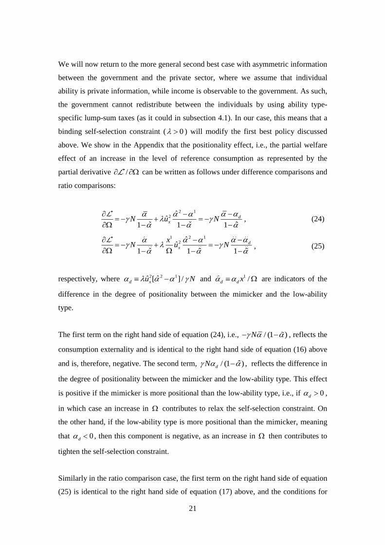
We will now return to the more general second best case with asymmetric information

between the government and the private sector, where we assume that individual

ability is private information, while income is observable to the government. As such,

the government cannot redistribute between the individuals by using ability type-

specific lump-sum taxes (as it could in subsection 4.1). In our case, this means that a

binding self-selection constraint ( 0 ) will modify the first best policy discussed

above. We show in the Appendix that the positionality effect, i.e., the partial welfare

effect of an increase in the level of reference consumption as represented by the

partial derivative / can be written as follows under difference comparisons and

ratio comparisons:

2 12 ˆ

ˆ1 1 1

dxN u N

, (24)

1 2 1

2 ˆˆ

1 1 1

dx

xN u N

, (25)

respectively, where 2 2 1ˆˆ [ ] /d xu N and 1 /d d x are indicators of the

difference in the degree of positionality between the mimicker and the low-ability

type.

The first term on the right hand side of equation (24), i.e., / (1 )N , reflects the

consumption externality and is identical to the right hand side of equation (16) above

and is, therefore, negative. The second term, / (1 )dN , reflects the difference in

the degree of positionality between the mimicker and the low-ability type. This effect

is positive if the mimicker is more positional than the low-ability type, i.e., if 0d ,

in which case an increase in contributes to relax the self-selection constraint. On

the other hand, if the low-ability type is more positional than the mimicker, meaning

that 0d , then this component is negative, as an increase in then contributes to

tighten the self-selection constraint.

Similarly in the ratio comparison case, the first term on the right hand side of equation

(25) is identical to the right hand side of equation (17) above, and the conditions for

22

when the second term reflecting self-selection effects is positive or negative are the

same as in the difference comparison case. However, note that the indicator of the

difference in the degree of positionality between the mimicker and the low-ability

type is here multiplied by the factor 1 /x . This adjustment is due to that each

individual’s marginal willingness to pay to avoid the externality depends directly on

this individual’s consumption in the ratio comparison case (which is given by 1x both

for low-ability individuals and mimickers).

To simplify the presentation, we introduce the following short notation for the second

term in parenthesis in equations (20) and (21):

'( )

( )

i ii

i i

f z x

f z w

.

As such, i reflects the relationship between and iz in the first best tax formulas

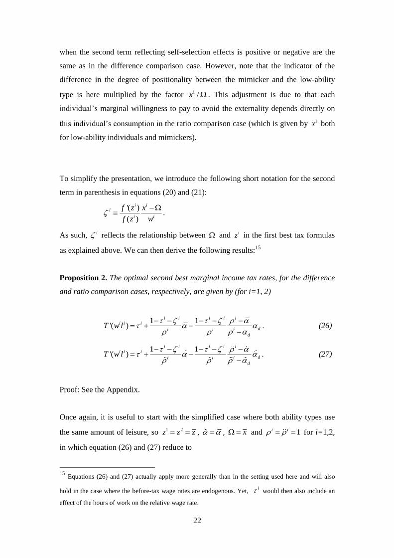
as explained above. We can then derive the following results:15

Proposition 2. The optimal second best marginal income tax rates, for the difference

and ratio comparison cases, respectively, are given by (for i=1, 2)

1 1'( )

i i i i ii i i

di i i

d

T w l

. (26)

1 1

'( )i i i i i

i i i

di i i

d

T w l

. (27)

Proof: See the Appendix.

Once again, it is useful to start with the simplified case where both ability types use

the same amount of leisure, so 1 2z z z , , x and 1i i for i=1,2,

in which equation (26) and (27) reduce to

15

Equations (26) and (27) actually apply more generally than in the setting used here and will also

hold in the case where the before-tax wage rates are endogenous. Yet, i would then also include an

effect of the hours of work on the relative wage rate.

23

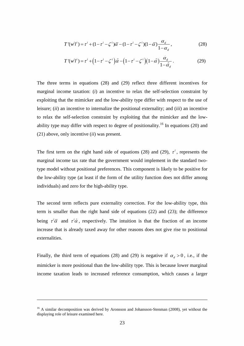
'( ) (1 ) (1 )(1 )1

i i i i i i i d

d

T w l

, (28)

'( ) 1 1 11

i i i i i i i d

d

T w l

. (29)

The three terms in equations (28) and (29) reflect three different incentives for

marginal income taxation: (i) an incentive to relax the self-selection constraint by

exploiting that the mimicker and the low-ability type differ with respect to the use of

leisure; (ii) an incentive to internalize the positional externality; and (iii) an incentive

to relax the self-selection constraint by exploiting that the mimicker and the low-

ability type may differ with respect to degree of positionality.16

In equations (20) and

(21) above, only incentive (ii) was present.

The first term on the right hand side of equations (28) and (29), i , represents the

marginal income tax rate that the government would implement in the standard two-

type model without positional preferences. This component is likely to be positive for

the low-ability type (at least if the form of the utility function does not differ among

individuals) and zero for the high-ability type.

The second term reflects pure externality correction. For the low-ability type, this

term is smaller than the right hand side of equations (22) and (23); the difference

being i and i , respectively. The intuition is that the fraction of an income

increase that is already taxed away for other reasons does not give rise to positional

externalities.

Finally, the third term of equations (28) and (29) is negative if 0d , i.e., if the

mimicker is more positional than the low-ability type. This is because lower marginal

income taxation leads to increased reference consumption, which causes a larger

16

A similar decomposition was derived by Aronsson and Johansson-Stenman (2008), yet without the

displaying role of leisure examined here.

24

utility loss for the mimicker than for the low-ability type.17

This, in turn, implies that

the self-selection constraint is relaxed. By analogy, if the low-ability type is more

positional than the mimicker, such that 0d , the third term is positive; in this case,

a decrease in the level of reference consumption contributes to a relaxation of the self-

selection constraint. Therefore, if 0d , the second and third terms on the right hand

side of equations (28) and (29) reinforce each other in the sense of jointly contributing

to higher marginal income tax rates. Finally, if 0d (in which case the mimicker

and the low-ability type do not differ with respect to the degree of positionality), the

third tax incentive vanishes; thus, positional concerns will only modify the second

best tax formula through the corrective tax component, which is proportional to the

average degree of positionality.

Note also that the tax regression result derived earlier will continue to hold under

certain conditions also in the context of equations (28) and (29). For instance, if the

self-selection effect caused by positional concerns does not dominate the effect of the

average degree of positionality, so that d , and if 1 0 (as in the original

Stiglitz 1982 model), then 1 1 2 2'( ) '( )T w l T w l . This will be discussed more

thoroughly below.18

Since equations (28) and (29) are analogous, we base the remaining interpretations on

equation (28). Note that the condition d always applies if the low-ability type is

at least as positional as the mimicker, in which case 0d . The intuition is, of

course, that the desire to internalize positional externalities and the incentive to relax

the self-selection constraint via policy-induced changes in the reference consumption,

i.e., incentives (ii) and (iii) referred to above, affect the optimal marginal income tax

rates in the same direction. However, even if the mimicker were more positional than

the low-ability type, meaning that 0d , the income tax structure would still be

17

Strictly speaking, this interpretation presupposes that 1 0d

in equation (28) and 1 0d

in

equation (29), which we assume here. 18

Notice that if d

, equation (28) reduces to the tax formula in the standard two-type model, i.e.

)'(i i ilT w . In this case, the tax structure will also be regressive (given that

1 2 ), yet for reasons

other than positional concerns. A similar argument applies to equation (29) if d

.

25

regressive in the sense mentioned above if the condition d applies. On the other

hand, if d , and if we continue to assume that 1 0 , then the marginal income

tax rate implemented for the low-ability type need no longer exceed the marginal

income tax rate implemented for the high-ability type; in fact, we cannot in this case

determine whether the low-ability type faces a higher or lower marginal income tax

rate than the high-ability type.

Returning to the general second best formulas in equations (26) and (27), what

remains is to analyze the effect of the variables i and i , which were equal to one

in the simplified case where both ability types use the same amount of leisure. This

component works in the same general way here as it did in the first best scenario

discussed above, with one important exception: It matters for the qualitative effect of

an increase or decrease in i whether exceeds or falls short of d in the difference

comparison case. Similarly, the effect of an increase in i in the ratio comparison

case depends on whether exceeds or falls short of d . To see this more clearly, let

us rewrite equations (26) and (27) as

'( ) (1 )i

i i i i d

i i

d d

T w l

, (30)

'( ) 1i

i i i i d

i i

d d

T w l

. (31)

To interpret equation (30), which is derived under the assumption of difference

comparisons, suppose that 1 0 , meaning that the low-ability type would face a

positive marginal income tax rate in the absence of any positional concerns. For the

high-ability type, the marginal income tax rate reduces to the second term on the right

hand side because 2 0 by the assumptions made earlier. Now, since 1 0 and

2 0 , and by adding the assumption that d , we again find that the condition

1 2 implies that the marginal income tax rate implemented for the low-ability

type exceeds that implemented for the high-ability type.

26

In the ratio comparison case, it correspondingly follows from equation (31) that if

1 /d d x , then 1 2 implies a larger marginal income tax rate for the

low-ability type than for the high-ability type. Moreover, we show in the Appendix

that the condition d implies d . Therefore, the following result is an

immediate consequence of Proposition 2:

Corollary 2. If 1 0 , d , and 1 2z z , then the income tax structure is

regressive in the sense that 1 1 2 2'( ) '( )T w l T w l for both the difference and the ratio

comparison cases.

The intuition behind Corollary 2 is straightforward: If 1 0 and d , we may

relax the self-selection constraint and internalize the positional externality by

implementing a higher marginal income tax rate for the low-ability type than for the

high-ability type.19

An important mechanism behind this result – captured by the

variables 1 0 and 2 0 – is that increased use of leisure by the low-ability type

contributes to reduce the positional externality, whereas increased use of leisure by

the high-ability type leads to an increase in the positional externality, ceteris paribus.

5. Extension: A more general measure of reference consumption

The analysis carried out so far assumes that the appropriate measure of reference

consumption at the individual level is given by a leisure-influenced consumption

average for the economy as a whole, , defined in Section 2. This approach is

analogous to earlier literature on public policy and relative consumption, where the

average consumption typically constitutes the reference point. However, it is plausible

that individuals may differ in their contributions to the reference consumption also for

reasons other than through the displaying role of leisure discussed above. For

19

To our knowledge, there is no empirical evidence on the basis of which one can sign d

. Hence, it

remains an open question whether low-ability individuals are more or less positional than potential

mimickers. Yet, recall that the (highly plausible) condition d

might be fulfilled even if the

mimicker is more positional than the low-ability type.

27

instance, Veblen (1899), Duesenberry (1949), and Schor (1998) have argued for the

importance of an asymmetry, such that “low-income groups are affected by

consumption of high-income groups but not vice versa” (Duesenberry, 1949, p. 101).

This is also consistent with the empirical findings of Bowles and Park (2005) that

more inequality in society tends to imply more work hours. Recent empirical evidence

by Corazzini, Esposito, and Majorano (forthcoming) suggests that people compare

both upwards and downwards, but that the upward comparison effect is stronger. In

the context of optimal taxation and relative consumption, Aronsson and Johansson-

Stenman (2010) and Micheletto (2011) address such “upward comparisons” as an

alternative to the conventional mean-value comparison yet without considering the

displaying role of leisure discussed here.

In this section, we allow for the asymmetry mentioned above while still retaining the

displaying role of leisure. To simplify the presentation, we will solely focus on the

difference comparison case in this section, although the qualitative insights are valid

also more generally. Moreover, we will continue to assume that the reference

consumption measure is the same for all individuals. Consider the following

generalized measure of reference consumption (which replaces the measure used

in earlier sections):

( )

( )

j j j j

j

j j j

j

n f z x

n f z

,

where [0,1]i for i=1,2, and 1j

j . The parameter i represents the weight

given to ability-type i's contribution to reference consumption. In other words, we

allow the ability types to differ with respect to their influences on the reference point.

Note that 2 1 implies that 2x , meaning that each individual only compares

himself/herself with the high-ability type. Similarly, 1 1 gives 1x , in which

case each individual only compares himself/herself with the low-ability type. The

analysis carried out in previous sections may, in turn, be interpreted as the special

case where 1 2 0.5 .

28

With the variable at our disposal, it is straightforward to generalize the expressions

for the marginal income tax rates in Proposition 2. Define

( )

(0,1)( )

i i ii

j j ji j

n f z

n f z

,

( )(1 ) 0

( )

j j j

ji

i i

n f z

f z N

, and

1 '( )

( )

ii i

i i

f zx

w f z ,

which replace the variables , i , and i , respectively, in the previous section, and

consider the following result:

Proposition 3. With the generalized measure of reference consumption, , the

marginal income tax rates can be written as (for i=1,2)

'( ) (1 )i

i i i i d

i i

d d

T w l

. (32)

Proof: See the Appendix.

Equation (32) has been written using the same format as equation (30), as this makes

it easy to relate equation (32) to Corollary 2. Equation (32) can be interpreted in the

same general way as equation (30); however, given that 1 0 and if d , as we

assumed in the interpretation of equation (30), the sufficient condition for a regressive

tax structure in Corollary 2, i.e., 1 2z z , must here be replaced with 1 2 . Even if

the high-ability type were to supply more labor than the low-ability type, this

condition becomes less likely to hold the larger the 2 relative to 1 . Therefore, with

“upward comparisons” in the sense that the leisure-weighted consumption by the

high-ability type has a more than proportional influence on the measure of reference

consumption, the case of regressive taxation becomes somewhat weaker than before.

To see this, let us consider the two special cases with 1 1 and 2 1 , respectively.

The following result is an immediate consequence of Proposition 3:

29

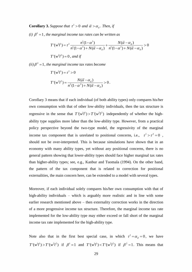
Corollary 3. Suppose that 1 0 and d . Then, if

(i) 1 1 , the marginal income tax rates can be written as

1 1

1 1 1

1 1 1 1

( )(1 )'( ) 0

(1 ) ( ) (1 ) ( )

d

d d

NnT w l

n N n N

2 2'( ) 0T w l , and if

(ii) 2 1 , the marginal income tax rates become

1 1 1'( ) 0T w l

2 2

2 2

( )'( ) 0

(1 ) ( )

d

d

NT w l

n N

.

Corollary 3 means that if each individual (of both ability types) only compares his/her

own consumption with that of other low-ability individuals, then the tax structure is

regressive in the sense that 1 1 2 2'( ) '( )T w l T w l independently of whether the high-

ability type supplies more labor than the low-ability type. However, from a practical

policy perspective beyond the two-type model, the regressivity of the marginal

income tax component that is unrelated to positional concerns, i.e., 1 2 0 ,

should not be over-interpreted. This is because simulations have shown that in an

economy with many ability types, yet without any positional concerns, there is no

general pattern showing that lower-ability types should face higher marginal tax rates

than higher-ability types; see, e.g., Kanbur and Tuomala (1994). On the other hand,

the pattern of the tax component that is related to correction for positional

externalities, the main concern here, can be extended to a model with several types.

Moreover, if each individual solely compares his/her own consumption with that of

high-ability individuals – which is arguably more realistic and in line with some

earlier research mentioned above – then externality correction works in the direction

of a more progressive income tax structure. Therefore, the marginal income tax rate

implemented for the low-ability type may either exceed or fall short of the marginal

income tax rate implemented for the high-ability type.

Note also that in the first best special case, in which 1 0d , we have

1 1 2 2'( ) '( )T w l T w l if 1 1 and 1 1 2 2'( ) '( )T w l T w l if 2 1 . This means that

30

upward comparisons give rise to a pattern of externality correction that works in the

direction of a more progressive income tax structure.

6. Conclusion

As far as we know, this is the first paper that has highlighted a displaying role of

leisure in the context of relative consumption comparisons when theoretically

analyzing optimal public policy. In line with Veblen (1899), we assume that leisure

has a displaying role in making relative consumption more visible. Our main results

are summarized as follows. First, increased consumption positionality typically

implies higher marginal income tax rates for both ability types. Second, the

consumption-displaying role of leisure provides an argument for regressive income

taxation in the sense that it contributes to increased marginal income taxation of the

low-ability type and decreased marginal income taxation of the high-ability type. This

is in contrast to the findings of Aronsson and Johansson-Stenman (forthcoming),

where concern for relative leisure implies an argument for progressive taxation. It is

also in contrast to a common statement in the popular debate, namely that concern for

relative consumption provides an argument in favor of more progressive income

taxation. Third, the levels of optimal marginal income tax rates – as well as whether

the tax system ought to be progressive or regressive – are largely dependent on how

the measure of reference consumption is determined. For example, if agents tend to

compare their own consumption more with that of high-ability than low-ability

individuals, this will influence the optimal tax structure in a progressive direction.

Future research may take several directions, and we briefly discuss some of these

directions below. First, our analysis assumes a competitive labor market and full

employment. However, as equilibrium unemployment is an important phenomenon in

real-world market economies, the use of leisure might not always be the outcome of

an optimal choice by the individual. It is, therefore, also relevant to combine the study

of optimal taxation in economies with positional preferences (at least if leisure plays a

role in this particular context) with imperfect competition in the labor market. Second,

instead of assuming that all aspects of private consumption are subject to positional

concerns (as we do here), another approach would be to distinguish between

31

positional and non-positional goods in the context of a mixed tax problem, where the

government has access both to a nonlinear income tax and linear commodity taxes.

Clearly, if the idea that leisure makes relative consumption more visible is applied to

such a framework, the principle of targeting would not apply. The reason is that the

ability types differ with respect to their contributions to the positional externality, in

which case a linear commodity tax is not a flexible enough instrument for externality

correction. Even if the commodity taxes were optimally chosen, our conjecture is that

the income tax is still likely to play a role reminiscent of that in the present paper, and

the mechanisms underlying the regressive income tax component would still remain.20

Third, the model here is of course, for analytical reasons, very stylized. While the

basic insights could be generalized to the case of many consumer types, as long as one

can apply sufficiently many marginal tax rates, the analytical results would not hold

when there are restrictions to, say, two or three different marginal tax rates. For this

and other generalizations we believe that simulations studies will provide important

insights regarding quantitative effects in more realistic settings. Finally, there is

clearly also room for more empirical research regarding relative consumption

comparisons in general, and regarding how reference consumption levels are

determined and the role of leisure in particular.

Appendix

Derivation of Equation (15)

Let us start with the marginal income tax rate facing the low-ability type. Combine

equations (11) and (12) to derive

1 2 1 2 1 1

, 1 1ˆ ˆ

z x x zMRS u n u n wx z

. (A1)

20

This conjecture is also based on insights from Micheletto (2008), who considers the problem of the

optimal tax mix based on a model with general consumption externalities, as well as on Eckerstorfer

(2011) and our own preliminary work dealing with relative consumption concerns with more than one

consumer good, yet without any consumption-displaying role of leisure.

32

Using 1 1 1 1 1

,'( ) z xT w l w w MRS from equation (8), substituting into equation (A1) and

rearranging, we obtain the expression for the marginal income tax rate of the low-

ability type. The marginal income tax rate of the high-ability type can be derived

analogously.

Derivation of Equations (16) and (24)

Start by differentiating the Lagrangean with respect to :

1 2 2ˆu u u

. (A2)

From equation (3) it follows in the difference comparison case according to equation

(1) that i iu v for i=1,2, and 2 2ˆ ˆu v . We can then use equation (5) to derive

i i i

xu u for i=1,2 (A3)

2 2 2ˆˆ ˆxu u . (A4)

Substituting equations (A3) and (A4) into equation (A2) gives

1 2 2 2 2ˆ ˆi

x x xu u u

. (A5)

Solving equation (12) for 1

xu and equation (14) for 2( ) xu and substituting into

equation (A5) gives

1 2 1 2 2 2 2

1 2ˆˆ ˆ

x xu n n ux x

. (A6)

Using / ( ) / ( )i i i j j

jx n f z n f z for i=1,2, substituting into equation (A6),

collecting terms, and rearranging gives equation (24). We can then derive equation

(16) as the special case where 0 .

33

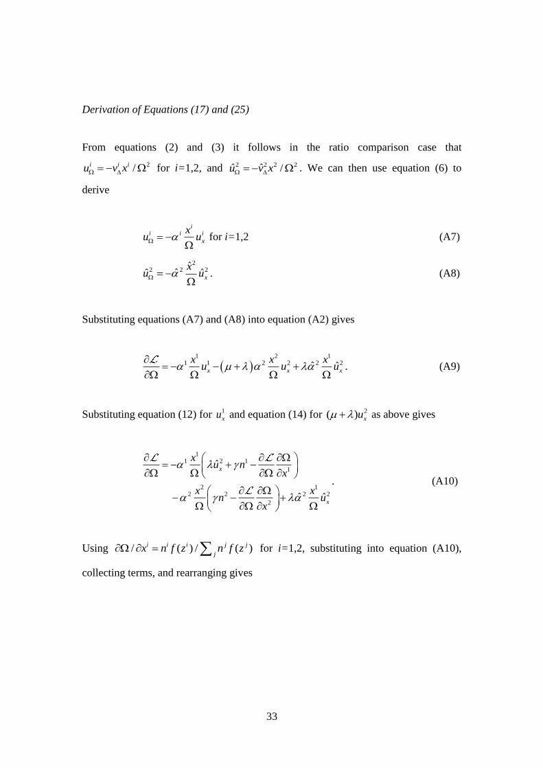
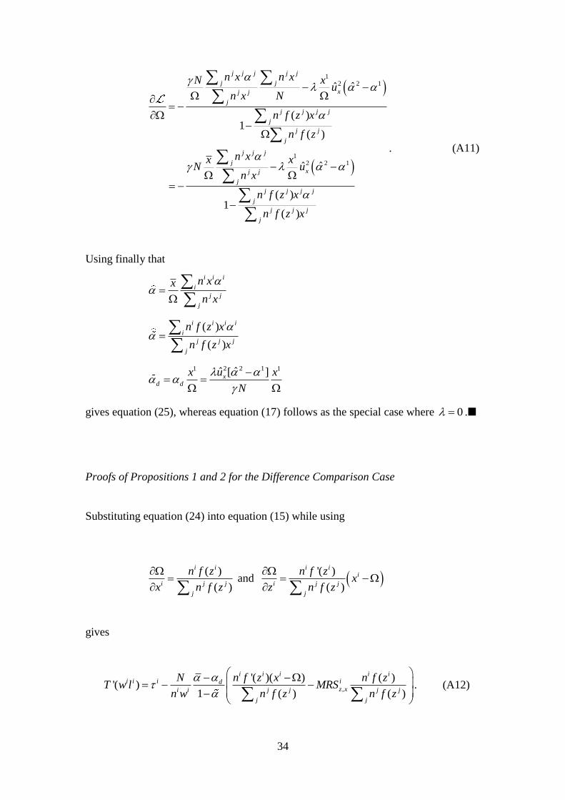
Derivation of Equations (17) and (25)

From equations (2) and (3) it follows in the ratio comparison case that

2/i i iu v x for i=1,2, and 2 2 2 2ˆ ˆ /u v x . We can then use equation (6) to

derive

i

i i i

x

xu u

for i=1,2 (A7)

2

2 2 2ˆˆˆ ˆ

x

xu u

. (A8)

Substituting equations (A7) and (A8) into equation (A2) gives

1 2 1

1 1 2 2 2 2ˆ ˆx x x

x x xu u u

. (A9)

Substituting equation (12) for 1

xu and equation (14) for 2( ) xu as above gives

11 2 1

1

2 12 2 2 2

2

ˆ

ˆ ˆ

x

x

xu n

x

x xn u

x

. (A10)

Using / ( ) / ( )i i i j j

jx n f z n f z for i=1,2, substituting into equation (A10),

collecting terms, and rearranging gives

34

12 2 1

12 2 1

ˆˆ

( )1

( )

ˆˆ

( )1

( )

j j j j j

j j

xj j

j

j j j j

j

j j

j

j j j

j

xj j

j

j j j j

j

j j j

j

n x n xN xu

n x N

n f z x

n f z

n xx xN u

n x

n f z x

n f z x

. (A11)

Using finally that

i i i

i

j j

j

n xx

n x

( )

( )

i i i i

i

j j j

j

n f z x

n f z x

2 2 11 1ˆˆ [ ]xd d

ux x

N

gives equation (25), whereas equation (17) follows as the special case where 0 .

Proofs of Propositions 1 and 2 for the Difference Comparison Case

Substituting equation (24) into equation (15) while using

( )

( )

i i

i j j

j

n f z

x n f z

and

'( )

( )

i ii

i j j

j

n f zx

z n f z

gives

,

'( )( ) ( )'( )

1 ( ) ( )

i i i i ii i i id

z xi i j j j j

j j

N n f z x n f zT w l MRS

n w n f z n f z

. (A12)

35

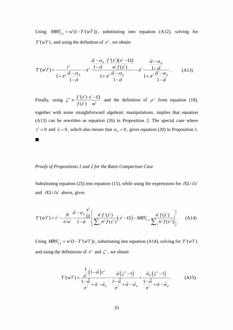
Using , (1 '( ))i i i i

z xMRS w T w l , substituting into equation (A12), solving for

'( )i iT w l , and using the definition of i , we obtain

'( )( )

1 ( ) 1'( )

1 1 11 1 1

i i

d di i i

i i i i

i i id d d

f z x

w f zT w l

. (A13)

Finally, using '( )

( )

i ii

i i

f z x

f z w

and the definition of i from equation (18),

together with some straightforward algebraic manipulations, implies that equation

(A13) can be rewritten as equation (26) in Proposition 2. The special case where

0i and 0 , which also means that 0d , gives equation (20) in Proposition 1.

Proofs of Propositions 1 and 2 for the Ratio Comparison Case

Substituting equation (25) into equation (15), while using the expressions for / ix

and / iz above, gives

1

,

'( ) ( )'( )

( ) ( )1

i i i idi i i i i

z xi i j j j j

j j

xN n f z n f z

T w l x MRSn w n f z n f z

. (A14)

Using , (1 '( ))i i i i

z xMRS w T w l , substituting into equation (A14), solving for '( )i iT w l

and using the definitions of i and i , we obtain

1

1 1 1'( )

1 1 1

ii i

i di i

d d di i i

T w l

. (A15)

36

Finally, using 1i

i

together with some straightforward algebraic

manipulations implies that equation (A15) can be rewritten as equation (27) in

Proposition 2. The special case where 0i and 0 , which also means that

0d , gives equation (21) in Proposition 1.

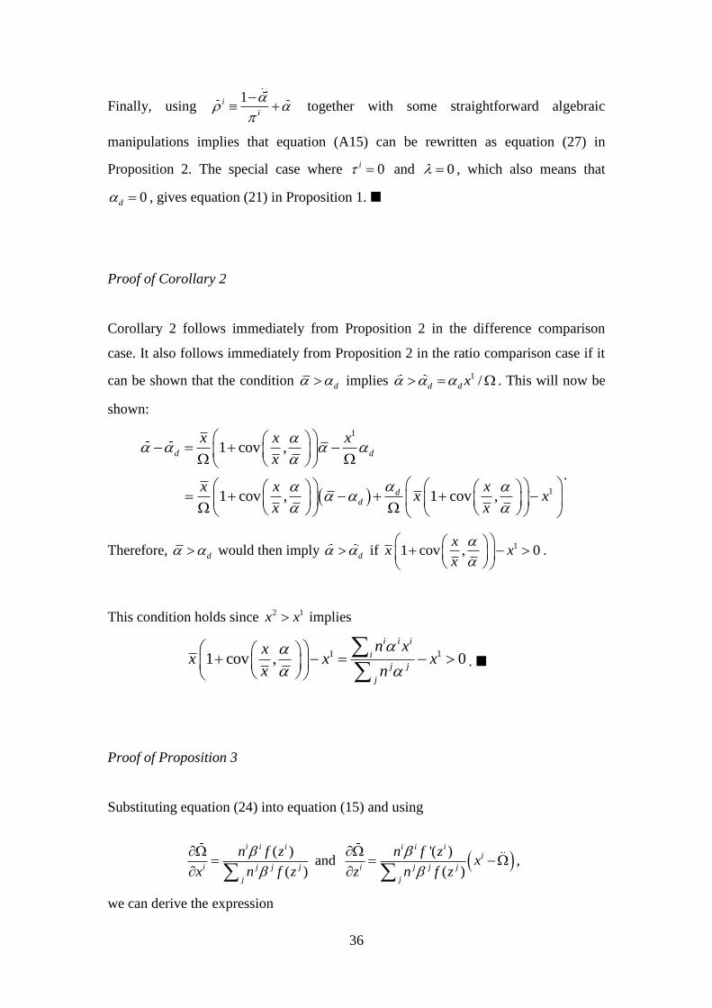
Proof of Corollary 2

Corollary 2 follows immediately from Proposition 2 in the difference comparison

case. It also follows immediately from Proposition 2 in the ratio comparison case if it

can be shown that the condition d implies 1 /d d x . This will now be

shown:

1

1

1 cov ,

1 cov , 1 cov ,

d d

dd

x x x

x

x x xx x

x x

.

Therefore, d would then imply d if 11 cov , 0x

x xx

.

This condition holds since 2 1x x implies

1 11 cov , 0

i i i

i

j j

j

n xxx x x

x n

.

Proof of Proposition 3

Substituting equation (24) into equation (15) and using

( )

( )

i i i

i j j j

j

n f z

x n f z

and

'( )

( )

i i ii

i j j j

j

n f zx

z n f z

,

we can derive the expression

37

,

'( )( ) ( )'( )

1 ( ) ( )

i i i i i i ii i i id

z xi i j j j j j j

j j

N n f z x n f zT w l MRS

n w n f z n f z

. (A16)

We can then use equation (A16) to derive equation (32) in exactly the same way as

we used equation (A12) to derive equation (26) in the proof of Proposition 2 above.

Proof of Corollary 3

In Corollary 3, it follows that 1/ 1x and 2 1 2/ / / 0x z z if

1 1 , while 2/ 1x and 1 1 2/ / / 0x z z if 2 1 . With this

modification, the marginal income tax rates in the corollary can be derived in the

same way as we derived equation (32).

References

Abel AB (2005) Optimal Taxation When Consumers Have Endogenous Benchmark

Levels of Consumption. Rev Eco Stud 72:1-19.

Akerlof GA (1997) Social Distance and Social Decisions. Econometrica 65:1005-

1027.

Alpizar F, Carlsson F, Johansson-Stenman O (2005) How Much Do We Care About

Absolute Versus Relative Income and Consumption? J Econ Behav Organ

56:405-421.

Aronsson T, Johansson-Stenman O (2008) When the Joneses’ Consumption Hurts:

Optimal Public Good Provision and Nonlinear Income Taxation. J Public Econ

92:986-997.

Aronsson T, Johansson-Stenman O (2010) Positional Concerns in an OLG Model:

Optimal Labor and Capital Income Taxation. Int Econ Rev 51:1071-1095.

38

Aronsson T, Johansson-Stenman O (forthcoming) Conspicuous Leisure: Optimal

Income Taxation When Both Relative Consumption and Relative Leisure

Matter. Scand J Econ.

Blanchflower DG, Oswald AJ (2004) Well-being over time in Britain and the USA. J

Public Econ 88:1359-1386.

Blumkin T, Sadka E (2007) A Case for Taxing Charitable Donations. J Public Econ

91:1555-1564.

Boskin MJ, Sheshinski E (1978) Individual Welfare Depends upon Relative Income.

Quart J Econ 92:589-601.

Bowles S, Park Y-J (2005) Inequality, Emulation, and Work Hours: Was Thorsten

Veblen Right? Econ J 15:F397-F413.

Brekke K-A, Howarth RB (2002) Affluence, Well-Being and Environmental Quality.

Cheltenham, Edward Elgar.

Carlsson F, Johansson-Stenman O, Martinsson P (2007) Do You Enjoy Having More

Than Others? Survey Evidence of Positional Goods. Economica 74:586-598.

Clark AE, Frijters P, Shields MA (2008) Relative Income, Happiness and Utility: An

Explanation for the Easterlin Paradox and Other Puzzles. J Econ Lit 46:95-144.

Clark A, Senik C (2010) Who Compares to Whom? The Anatomy of Income

Comparisons in Europe. Econ J 120:573-594.

Cole HL, Mailath GJ, Postlewaite A (1992) Social Norms, Savings Behavior, and

Growth. J Polit Economy 100:1092-1125.

Cole HL, Mailath GJ, Postlewaite A (1998) Class Systems and the Enforcement of

Social Norms. J Public Econ 70:5-35.

Corazzini L, Esposito L, Majorano F (forthcoming) Reign in Hell or Serve in Heaven?

A Cross-country Journey into the Relative vs Absolute Perceptions of

Wellbeing. J Econ Behav Organ.

Corneo G, Jeanne O (1997) Conspicuous Consumption, Snobbism and Conformism.

J Public Econ 66:55-71.

Corneo G, Jeanne O (2001) Status, the Distribution of Wealth, and Growth. Scand J

Econ 103:283-293.

Dohmen T, Falk A, Fliessbach K, Sunde U, Weber B (forthcoming) Relative versus

absolute income, joy of winning, and gender: Brain imaging evidence. J Public

Econ.

39

Duesenberry JS (1949) Income, Saving and the Theory of Consumer Behavior.

Harvard Univeristy Press, Cambridge, MA.

Dupor B, Liu WF (2003) Jealousy and Overconsumption. Amer Econ Rev 93:423-

428.

Easterlin RA (2001) Income and Happiness: Towards a Unified Theory. Econ J

111:465-484.

Eckerstorfer P (2011) Relative Consumption Concerns and the Optimal Tax Mix.

Working paper 1114, Department of Economics, University of Linz, Austria.

Ferrer-i-Carbonell A (2005) Income and Well-being: An Empirical Analysis of the

Comparison Income Effect. J Public Econ 89:997-1019.

Fliessbach K, Weber B, Trautner P, Dohmen T, Sunde U, Elger CE, Falk A (2007)

Social Comparison Affects Reward-Related Brain Activity in the Human

Ventral Striatum. Science 318:1305-1308.

Frank RH (1985) The Demand for Unobservable and Other Nonpositional Goods.

Amer Econ Rev 75:101-116.

Frank RH (2005) Positional Externalities Cause Large and Preventable Welfare

Losses. Amer Econ Rev 95:137-141.

Frank RH (2008) Should Public Policy Respond to Positional Externalities? J Public

Econ 92:1777-1786.

Hopkins E, Kornienko T (2004) Running to Keep in the Same Place: Consumer

Choice as a Game of Status. Amer Econ Rev 94:1085-1107.

Hopkins E, Kornienko T (2009) Status, Affluence, and Inequality: Rank-Based

Comparisons in Games of Status. Games Econ Behav 67:552-568.

Ireland NJ (2001) Optimal Income Tax in the Presence of Status Effects. J Public

Econ 81:193-212.

Johansson-Stenman O, Carlsson F, Daruvala D (2002) Measuring Future

Grandparents' Preferences for Equality and Relative Standing. Econ J 112:362-

383.

Kanbur R, Tuomala M (1994) Inherent Inequality and the Optimal Graduation of

Marginal Tax Rates. Scand J Econ 96:275-82.

Kanbur R, Tuomala M (2010) Relativity, Inequality and Optimal Nonlinear Income

Taxation. Working paper, Cornell University.

Layard R (1980) Human Satisfaction and Public Policy. Econ J 90:737-750.

40

Ljungqvist L, Uhlig H (2000) Tax Policy and Aggregate Demand Management Under

Catching Up with the Joneses. Amer Econ Rev 90:356-366.

Luttmer EFP (2005) Neighbors as Negatives: Relative Earnings and Well-Being.

Quart J Econ 120:963-1002.

Micheletto L (2008) Redistribution and Optimal Mixed Taxation in the Presence of

Consumption Externalities. J Public Econ 92:2262-2274.

Micheletto L (2011) Optimal Nonlinear Redistributive Taxation and Public Good

Provision in an Economy with Veblen Effects. J Public Econ Theory 13:71-96.

Ng Y-K (1987) Relative Income Effects and the Appropriate Level of Public

Expenditure. Oxford Econ Pap 39:293-300.

Oswald A (1983) Altruism, Jealousy and the Theory of Optimal Non-Linear Taxation.

J Public Econ 20:77-87.

Rayo L, Becker GS (2007) Evolutionary Efficiency and Happiness. J Polit Economy

115:302-337.

Samuelson L (2004) Information-Based Relative Consumption Effects. Econometrica

72:93-118.

Schor J (1998) The Overspent American. New York: Haperperennial.

Solnick S, Hemenway D (2005) Are Positional Concerns Stronger in Some Domains

than in Others? Amer Econ Rev, Papers and Proceedings 45:147-151.

Stern NH (1982) Optimum Taxation with Errors in Administration. J Public Econ

17:181-211.

Stevenson B, Wolfers J (2008) Economic Growth and Subjective Well-Being:

Reassessing the Easterlin Paradox. Brookings Pap Econ Act, Spring, 1-87.

Stiglitz JE (1982) Self-Selection and Pareto Efficient Taxation. J Public Econ 17:213-

240.

Tuomala M (1990) Optimal Income Tax and Redistribution. Clarendon Press, Oxford.

Veblen T (1899) The Theory of the Leisure Class. New York: Macmillan.

Wendner R, Goulder LH (2008) Status Effects, Public Goods Provision, and the

Excess Burden. J Public Econ 92:1968-1985.

Wendner R (2010) Conspicuous Consumption and Generation Replacement in a

Model with Perpetual Youth. J Public Econ 94:1093-1107.

Wendner R (2011) Will the Consumption Externalities' Effects in the Ramsey Model

Please Stand Up? Econ Letters 111:210-212.