Variable Speed Control of Wind Turbines Based on the Quasi ... filecoupling, as well as external interference, present great challenges in wind turbine controller design. In this paper,

energies

Article

Variable Speed Control of Wind Turbines Based onthe Quasi-Continuous High-Order SlidingMode Method

Yanwei Jing 1, Hexu Sun 1, Lei Zhang 1 and Tieling Zhang 2,*1 School of Control Science and Engineering, Hebei University of Technology, Hongqiao District,

Tianjin 300131, China; [email protected] (Y.J.); [email protected] (H.S.);[email protected] (L.Z.)

2 School of Mechanical, Materials, Mechatronic and Biomedical Engineering, University of Wollongong,Wollongong, NSW 2522, Australia

* Correspondance: [email protected]; Tel.: +61-2-4221-4821

Received: 11 September 2017; Accepted: 12 October 2017; Published: 17 October 2017

Abstract: The characteristics of wind turbine systems such as nonlinearity, uncertainty and strongcoupling, as well as external interference, present great challenges in wind turbine controller design.In this paper, a quasi-continuous high-order sliding mode method is used to design controllers due toits strong robustness to external disturbances, unmodeled dynamics and parameter uncertainties. Itcan also effectively suppress the chattering toward which the traditional sliding mode control methodis ineffective. In this study, the strategy of designing speed controllers based on the quasi-continuoushigh order sliding mode method is proposed to ensure the wind turbine works well in different windmodes. First, the plant model of the variable speed control system is built as a linearized model; andthen a second order speed controller is designed for the model and its stability is proved. Finally, thedesigned controller is applied to wind turbine pitch control. Based on the simulation results from asimulation of 1200 s which contains almost all wind speed modes, it is shown that the pitch angle canbe rapidly adjusted according to wind speed change by the designed controller. Hence, the outputpower is maintained at the rated value corresponding to the wind speed. In addition, the robustnessof the system is verified. Meanwhile, the chattering is found to be effectively suppressed.

Keywords: wind turbine; quasi-continuous high-order sliding mode control; variable speed control;pitch control

1. Introduction

The technical development of wind power is partially represented by the development of windturbine control technology. Various control methods such as robust control, adaptive control, backstepping control, sliding mode control, model predictive control and so on have been proposedand studied [1–5]. Among these methods, sliding mode control has been proven to be robust withrespect to system parameter variations and external disturbances, and it can quickly converge to thecontrol target.

In practical application, proportional integral derivative (proportional integral differential, PID)controller or proportional integral (PI) controllers are widely applied. In these the controller parametersare obtained based on experience and/or on-site testing as no theoretical system is used for thecalculation, thereby lacking a proved stability and causing security risk. The ultimate goal to controlwind turbine is to provide safe and stable operation in the whole process, to reach the regional specificcontrol objectives, and to provide safe and reliable power production. Therefore, the study of advanced,intelligent, stable, and secure control technology has become so important [6] that many scholars

Energies 2017, 10, 1626; doi:10.3390/en10101626 www.mdpi.com/journal/energies

http://www.mdpi.com/journal/energies

http://www.mdpi.com

http://dx.doi.org/10.3390/en10101626

http://www.mdpi.com/journal/energies

Energies 2017, 10, 1626 2 of 21

worldwide have made efforts to develop new control techniques, especially control techniques appliedto pitch control.

In the early studies, the classical P/PI/PID pitch angle controllers based on linearized modelshave been implemented [7–10]. In those studies, however, wind turbine control design is based onexperimental models [11]. A simple control scheme for variable speed wind turbines is given in [12],and a comparison of nonlinear and linear model-based design of variable speed wind turbines ispresented in [13].

In [14,15], the use of integral sliding-mode control method combined with the improvedNewton-Raphson wind speed estimator is proposed to design the controller to control the generatortorque so as to adjust the rotor speed for achieving the maximum energy conversion of the windturbine. The control stability is investigated by the Lyapunov function analysis. In order to maximizethe efficiency of energy conversion and reduce mechanical stress of main shaft, in [16], an adaptivesecond order sliding mode control strategy with variable gain is formulated through improvementof the super-twisting algorithm. This control strategy is able to deal with the randomness of windspeed, the non-linearity of wind turbine systems, uncertainty of the model and the influence ofexternal disturbances.

In [17], the traditional sliding mode control strategy is used to control the power of a variablespeed wind turbine. The ideal feedback control tracking under uncertain and disturbing conditionsis realized, which ensures the stability of the two operating regions and the strong robustness of thecontrol system. Reference [18] proposed a high-order sliding mode control method for power control.The algorithm is simple and reliable, and the generator torque chattering is small, thereby greatlyimproving the efficiency of wind energy conversion. Reference [19] proposed a continuous high-ordersliding mode control method for nonlinear control of the variable speed wind turbine system, which iscombined with the maximum power point tracking (MPPT) algorithm to ensure the optimal poweroutput tracking, better system dynamic performance and strong robustness.

The randomness and uncertainty of wind speed, the non-linearity of wind turbine systems andthe presence of external disturbances make it difficult to establish accurate mathematical models formodelling the wind turbine subsystems. Under this situation and owing to the strong robustness ofthe control method to external disturbances, unmodeled dynamics and parameter uncertainties; thesliding mode control has been widely utilized. In addition, the control method has advantages ofsimple control law and fast dynamic response. As the traditional sliding mode control is prone tosevere chattering, it is difficult to maintain the system stability. As a result, it is only applicable to therelative order 1 system. In order to overcome the issue, this paper proposes a high-order sliding modecontrol method for pitch control and speed control of the wind turbines. This method can effectivelyweaken the chattering phenomenon and realize any order control while achieving the traditionalcontrol target.

The remainder of this paper is organized as follows: Section 2 introduces the sliding mode controlmethod, Section 3 describes the control models, Section 4 presents the design of the controllers and itsstability, and Section 5 discusses the simulation results. Finally, it is concluded as shown in Section 6.

2. Introduction to High-Order Sliding Mode Control

2.1. Conventional Sliding Mode Control

Sliding mode control is defined and described in [20]. It is a nonlinear control method that altersthe dynamics of a nonlinear system by application of a discontinuous control signal that forces thesystem to “slide” along a cross-section of the system’s normal behavior. However, the conventionalsliding mode control has the following shortcomings.

Energies 2017, 10, 1626 3 of 21

2.1.1. Chattering ωls

The sliding mode motion causes the state of the system to continue to move up and down ata low amplitude and high frequency along a predetermined trajectory, but the actual sliding modedoes not occur strictly on the sliding surface due to the inertia and hysteresis of the switching device,thereby triggering a high-frequency switching of the control, resulting in chattering [21]. This kind ofchattering phenomenon will not only reduce the accuracy of system control and increase the energyloss, but also easily stimulate the high frequency unmodeled dynamics resulting in damage of thesystem stability and even damage of the controlled device.

2.1.2. Limited Relative Order

The conventional sliding mode control can only be applied to systems with relative order 1, i.e.,the control variable must appear explicitly on the sliding surface.

2.1.3. Low Control Accuracy

For discrete conventional sliding mode control systems, the system sliding error is proportionalto the sampling time, that is, the accuracy of the system state remaining in the sliding mode is the firstorder infinitesimal of the sampling time.

2.2. High-Order Sliding Model Control

In 2003, Levant [22] proposed a sliding mode control method with finite-time convergencefor system with arbitrary relative order and a quasi-continuous high-order sliding mode control(QCHOSM) method, in which the proposed high-order sliding mode controller is the commonconvergent controller in the finite time. It is used to control any uncertain system with arbitraryrelative order with the advantages of short convergence time and strong robustness.

For a single input and single output system:

.x(t) = f (t, x) + g(t, x)u (1)

where x(t) is system state vector and u is input of the control, with relative order of r of sliding surfaces(t, x) = 0, the control target is to make the system state move to s(t, x) = 0 within a limited time in therth order sliding mode. This means that:

s =.s =

..s = · · · = s(r−1) = 0. (2)

If r is known in the system, the following is obtained:

s(r) = h(t, x) + g(t, x)u (3)

where h(t, x) = s(r)∣∣∣u=0

, g(t, x) = ∂∂u s(r) 6= 0. And there exist Km, KM, and C > 0 for [14]:

0 ≤ Km ≤∂

∂us(r) ≤ KM (4)

where∣∣∣ s(r)∣∣∣

u=0

∣∣∣ ≤ 0.

When Equation (1) is true, any continuous input u = U(

s,.

s, · · · s(r−1))

satisfies U(0, 0, · · · , 0) =

−h(t, x)/g(t, x) for s ≡ 0. Because of uncertain factors existing in the system, u = U(

s,.

s, · · · s(r−1))

in

Equation (1) is not continuous at least, then it can be converged to s(r) [19,20]. From Equations (3) and(4), the following solution exits in Filippov:

s(r) ∈ [−C, C] + [Km, KM]u. (5)

Energies 2017, 10, 1626 4 of 21

In summary, r-order sliding mode control is defined as design the sliding surface s, and constructthe discontinuous controller u = U(s,

.s, · · · s(r−1)) to make the system trajectory finally stabilize

onto s(r).For any order sliding mode control with q being a positive constant and q ≥ r, Levant [22]

proposed the following control equations:

N1,r = |s|(r−1)/r

Ni,r =

(|s|q/r +

∣∣ .s∣∣q/(r−1)

+ · · ·+∣∣∣s(i−1)

∣∣∣q/(r−i+1))(r−i)/q

Nr−1,r =

(|s|q/r +

∣∣ .s∣∣q/(r−1)

+ · · ·+∣∣∣s(r−2)

∣∣∣q/2)1/q

, i = 1, 2, · · · , r

φ0,r = sφ1,r =

.s + β1N1,rsgn(s)

φi,r = s(i) + βi Ni,rsgn(φi−1,r), i = 1, 2, · · · , r− 1

(6)

where β1, β2, . . . , βr−1 are positive and obtained by simulation tests.

Theorem 1. Assume the system expressed by Equation (1) has the relative order r on s and satisfies Equation (5),and its trajectory can be unlimitedly extended in time for any order Lebesgue measurable and bounded control,the control law:

u = −k · sgn(

φr−1, r(s,.s, · · · s(r−1))

)(7)

is able to ensure that the r-order sliding mode converged in finite time exists, and the convergence time is thelocally bounded function of the initial condition for appropriately determined positive values of β1, β2, . . . ,βr−1 and k.

For the system with relative order r which is less than 4, the controller expression was presentedin [23] as follows:

(1) u = −k · sgns(2) u = −k(

.s + |s|1/2sgns)/(

∣∣ .s∣∣+ |s|1/2)

(3) u = −k..s+2(| .s|+|s|2/3)

−1/2(

.s+|s|2/3sgns)

|..s|+2(| .s|+|s|2/3)1/2

(4) ϕ3,4 =..s + 3

[..s + (

∣∣ .s∣∣+ 0.5|s|3/4)

−1/3(

.s + 0.5|s|3/4sgns)

][∣∣..s∣∣+ (∣∣ .s∣∣+ 0.5|s|3/4)

2/3]−1/2

N3,4 =..s + 3

[∣∣..s∣∣+ (∣∣ .s∣∣+ 0.5|s|3/4)

2/3]1/2

u = −kϕ3,4/N3,4

(8)

which is derived from Equations (6) and (7).Through high-order sliding mode, the control algorithm can be constructed on any order

derivative of the sliding mode. However, the calculation of the control algorithm requires theinformation of the derivative of the previous order system variables. For example, the controller(8) needs the sliding surface and its real-calculated value or direct measure of its real time derivativeswith respect to time. However, the higher order derivatives of these state variables do not necessarilyhave physical meaning and the sensitivity to noise makes these higher order derivatives not be directlymeasured by the sensor [24]. In order to solve these problems, Levant designed a finite time-convergentrobust differentiator with high precision by considering the effect of noise based on the high-ordersliding mode theory.

In practical application of high-order sliding mode, the value of the sliding surface and its firstderivative can be estimated by Levant Robust Differentiator:

u = −k · sgn(φr−1, r(z0, z1, · · · zr−1)) (9)

Energies 2017, 10, 1626 5 of 21

where z0, z1, · · · , zr−1 are sliding surface and derivatives, respectively. Levant sliding differentiatoris constituted by a first order differentiator in real time as [25]:

.z0 = υ0

υ0 = −λrL1/r|z0 − s|(r−1)/rsgn(z0 − s) + z1.zk = υk

υk = −λr−kL1/(r−k)|zk − υk−1|(r−k−1)/(r−k)sgn(zk − υk−1) + zk+1 , k = 1, · · · , r− 2.zr−1 = −λ1Lsgn(zr−1 − υr−2)

(10)

The values of k in Equations (7) and (8), and value of L in Equation (10) are obtained by simulation.L in Equation (10) should be large enough to ensure that the system has good performance in thepresence of measurement error. Usually in the simulation the following parameter values are used:L = 400, λ1 = 1.1, λ2 = 1.5, λ3 = 2.0, λ4 = 3.0, λ5 = 5.0 and λ6 = 8.0 [25].

3. Models of Variable Speed Controller

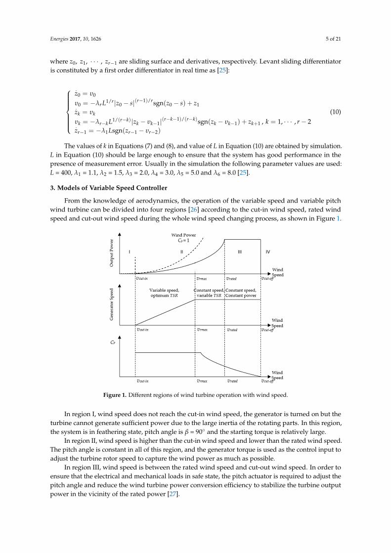
From the knowledge of aerodynamics, the operation of the variable speed and variable pitchwind turbine can be divided into four regions [26] according to the cut-in wind speed, rated windspeed and cut-out wind speed during the whole wind speed changing process, as shown in Figure 1.

Energies 2017, 10, 1626 5 of 20

0 0( 1) /1/

0 0 0 1

( 1) / ( )1/ ( )1 1 1

1 1 1 2

sgn( )

sgn( ) , 1, , 2sgn( )

r rrr

k k

r k r kr kk r k k k k k k

r r r

z

L z s z s z

z

L z z z k r

z L z

υ

υ λυ

υ λ υ υλ υ

−

− − −−− − − +

− − −

=

= − − − + =

= − − − + = − = − −

(10)

The values of k in Equations (7) and (8), and value of L in Equation (10) are obtained by simulation. L in Equation (10) should be large enough to ensure that the system has good performance in the presence of measurement error. Usually in the simulation the following parameter values are used: L = 400, λ1 = 1.1, λ2 = 1.5, λ3 = 2.0, λ4 = 3.0, λ5 = 5.0 and λ6 = 8.0 [25].

3. Models of Variable Speed Controller

From the knowledge of aerodynamics, the operation of the variable speed and variable pitch wind turbine can be divided into four regions [26] according to the cut-in wind speed, rated wind speed and cut-out wind speed during the whole wind speed changing process, as shown in Figure 1.

In region I, wind speed does not reach the cut-in wind speed, the generator is turned on but the turbine cannot generate sufficient power due to the large inertia of the rotating parts. In this region, the system is in feathering state, pitch angle is β = 90° and the starting torque is relatively large.

In region II, wind speed is higher than the cut-in wind speed and lower than the rated wind speed. The pitch angle is constant in all of this region, and the generator torque is used as the control input to adjust the turbine rotor speed to capture the wind power as much as possible.

In region III, wind speed is between the rated wind speed and cut-out wind speed. In order to ensure that the electrical and mechanical loads in safe state, the pitch actuator is required to adjust the pitch angle and reduce the wind turbine power conversion efficiency to stabilize the turbine output power in the vicinity of the rated power [27].

In region IV, wind speed is higher than the cut-out wind speed. Cut-out speed is the maximum speed of the wind for power production. When wind speed is higher than the cut-out speed, the wind turbine is shut down without any power production; otherwise, it will lead to damage to the wind turbine.

In this paper, the controllers are designed for pitch control with wind speed in the regions from II to IV.

Figure 1. Different regions of wind turbine operation with wind speed. Figure 1. Different regions of wind turbine operation with wind speed.

In region I, wind speed does not reach the cut-in wind speed, the generator is turned on but theturbine cannot generate sufficient power due to the large inertia of the rotating parts. In this region,the system is in feathering state, pitch angle is β = 90 and the starting torque is relatively large.

In region II, wind speed is higher than the cut-in wind speed and lower than the rated wind speed.The pitch angle is constant in all of this region, and the generator torque is used as the control input toadjust the turbine rotor speed to capture the wind power as much as possible.

In region III, wind speed is between the rated wind speed and cut-out wind speed. In order toensure that the electrical and mechanical loads in safe state, the pitch actuator is required to adjust thepitch angle and reduce the wind turbine power conversion efficiency to stabilize the turbine outputpower in the vicinity of the rated power [27].

Energies 2017, 10, 1626 6 of 21

In region IV, wind speed is higher than the cut-out wind speed. Cut-out speed is the maximumspeed of the wind for power production. When wind speed is higher than the cut-out speed, thewind turbine is shut down without any power production; otherwise, it will lead to damage to thewind turbine.

In this paper, the controllers are designed for pitch control with wind speed in the regions from IIto IV.

3.1. Wind Turbine Model

From aerodynamics, the mechanical power captured by the wind turbine from wind energy isknown as [28]:

Pa =12

ρπR2Cp(λ, β)v3 (11)

where Cp(λ, β) represents the wind turbine power conversion efficiency, used to characterize theefficiency of the wind turbine converting wind energy to mechanical energy, which is associated withtip speed ratio λ and pitch angle β, and is defined as [2]:

Cp(λ, β) = c1(c2

λi− c3β− c4)e

− c5λi + c6λ (12)

with:1λi

=1

λ + 0.08β− 0.035

β3 + 1(13)

and c1 = 0.5176, c2 = 116, c3 = 0.40, c4 = 5.0, c5 = 21.0, c6 = 0.0068 [2]. The values of coefficients c1 to c6

depend on the specific environment, the turbine blade shape profile and its aerodynamic performance.λ is calculated as:

λ = Rωr

v(14)

where ωr is turbine rotor speed (rad/s). For different pitch angle values, there is an optimal tip speedratio λopt, making it work continuously along with the change of wind speed on the best workingpoint, then the wind turbine conversion efficiency is the highest.

The mechanical power expressed in terms of aerodynamic torque is shown in Equation (15):

Pa = ωrTa (15)

where Ta is aerodynamic torque (N·m), defined as:

Ta =12

πρR3 Cp(λ, β)

λv2. (16)

3.2. Generator Model

In addition to considering the reliability and operating life of the generator, it is also necessaryto consider whether it can adapt to the different changes of wind conditions and provide stableelectrical energy.

In pitch control, it is to adjust the pitch angle with response to the required generator outputtorque and rotational speed in order to maintain a constant state. For the commonly used asynchronousgenerator, the generator torque is expressed as [29]:

Te =gm1U2

1r2′

(ωg −ω1)[(r1 − C1ωg−ω1

)2+ (x1 + C1x2′)2]

, (17)

ωg = ngωr. (18)

Energies 2017, 10, 1626 7 of 21

When wind speed is above the rated wind speed, it is necessary to start the propeller actuatorto restrict the wind energy captured by considering the load bearing capacity of the wind turbineand the limitation of the performance index of each component. The pitch control system adjusts thepitch angle which is determined by the wind speed. The blade pitch is driven by the servo motor. Itsmathematical model is given below:

τβ

.β = β∗ − β (19)

where β∗ is the reference value of the pitch angle (); β is the actual output pitch angle (), and τβ

is a time constant. This is actually a first-order delay link because the drive system itself has somecomputing delay, conditional delay, etc. so that the propeller actuator cannot do real-time response [27].The rotor actuator model can also be expressed as:

Gp(s) =β(s)β∗(s)

=1

τβs + 1. (20)

In summary, the control strategy for the variable speed stage is obtained in the following way,i.e., when the wind speed is lower than the rated wind speed, the generator torque is controlled sothat the turbine rotor speed can be adjusted quickly to find the best power output point and maximizethe wind energy conversion efficiency. The wind turbine speed control scheme is shown in Figure 2,where Pa represents the power captured by the wind turbine from the wind.

Energies 2017, 10, 1626 7 of 20

βτ β β β∗= − (19)

where *β is the reference value of the pitch angle (°); β is the actual output pitch angle (°), and is a time constant. This is actually a first-order delay link because the drive system itself has some computing delay, conditional delay, etc. so that the propeller actuator cannot do real-time response [27]. The rotor actuator model can also be expressed as:

( ) 1( )1( )p

sG s

ss β

βτβ ∗= =

+. (20)

In summary, the control strategy for the variable speed stage is obtained in the following way, i.e., when the wind speed is lower than the rated wind speed, the generator torque is controlled so that the turbine rotor speed can be adjusted quickly to find the best power output point and maximize the wind energy conversion efficiency. The wind turbine speed control scheme is shown in Figure 2, where Pa represents the power captured by the wind turbine from the wind.

Figure 2. Variable speed control scheme for wind turbine.

3.3. Nonlinear-Controlled Object Model

In the condition of a control system involving the model uncertainty and external disturbance, and the wind speed is higher than the rated wind speed; variable pitch control is utilized to which a newly proposed quasi-continuous high order sliding mode control method is applied. The control system design needs to take into account the following aspects: pitch control strategy, the controlled object model, accurate feedback linearization, controller design, stability verification and simulation analysis.

The controlled object model of wind turbine is expressed by Equation (21) [18]:

( ) ( )

r r a ls r r

lsg g g g e

g

g gls ls r ls r

g g

J T T K

TJ K T

n

T K Bn n

ω ω

ω ω

ω ωω ω

= − − = − − = − + −

(21)

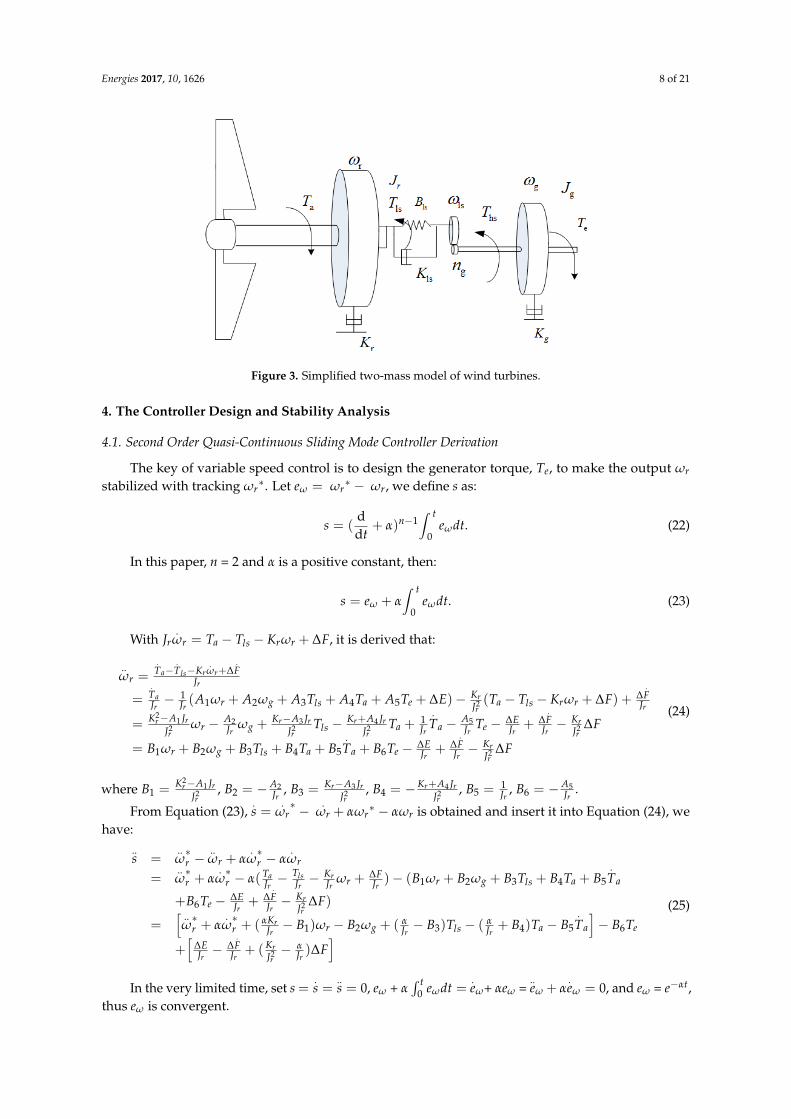
where Jr is the turbine rotor moment of inertia; Kr is damping coefficient of turbine rotor (N·m/rad/s); Jg is generator inertia (kg·m2); Kg is generator external damping coefficient (N·m/rad/s); ng is gearbox ratio. This model is built based on a simplified two-mass model of horizontal axis wind turbines as shown in Figure 3. The power drivetrain system of this type of wind turbines includes turbine rotor, main shaft, gearbox and generator.

Figure 2. Variable speed control scheme for wind turbine.

3.3. Nonlinear-Controlled Object Model

In the condition of a control system involving the model uncertainty and external disturbance, andthe wind speed is higher than the rated wind speed; variable pitch control is utilized to which a newlyproposed quasi-continuous high order sliding mode control method is applied. The control systemdesign needs to take into account the following aspects: pitch control strategy, the controlled objectmodel, accurate feedback linearization, controller design, stability verification and simulation analysis.

The controlled object model of wind turbine is expressed by Equation (21) [18]:Jr

.ωr = Ta − Tls − Krωr

Jg.

ωg = Tlsng− Kgωg − Te

.Tls = Kls(ωr −

ωgng) + Bls(

.ωr −

.ωgng)

(21)

where Jr is the turbine rotor moment of inertia; Kr is damping coefficient of turbine rotor (N·m/rad/s);Jg is generator inertia (kg·m2); Kg is generator external damping coefficient (N·m/rad/s); ng is gearboxratio. This model is built based on a simplified two-mass model of horizontal axis wind turbines asshown in Figure 3. The power drivetrain system of this type of wind turbines includes turbine rotor,main shaft, gearbox and generator.

Energies 2017, 10, 1626 8 of 21Energies 2017, 10, 1626 8 of 20

Figure 3. Simplified two-mass model of wind turbines.

4. The Controller Design and Stability Analysis

4.1. Second Order Quasi-Continuous Sliding Mode Controller Derivation

The key of variable speed control is to design the generator torque, Te, to make the output stabilized with tracking ∗. Let = ∗ − , we define s as:

1

0

d( )d

tns e dtt ωα −= + . (22)

In this paper, n = 2 and α is a positive constant, then:

0

ts e e dtω ωα= + . (23)

With = − − + ∆ , it is derived that:

1 2 3 4 5 2

23 51 2 4

2 2 2 2

1 2 3 4 5

1 ( ) ( )

1

a ls r rr

r

a rr g ls a e a ls r r

r r rr

r rr r r r rr g ls a a e

r r r r rr r r r

r g ls a

T T K F

J

T K FA A AT A T AT E T T K F

J J JJ

K A J AK A J A K A J KE FT T T T F

J J J J JJ J J J

B B B T B T B T

ωω

ω ω ω

ω ω

ω ω

− − + Δ=

Δ= − + + + + + Δ − − − + Δ +

−− + Δ Δ= − + − + − − + − Δ

= + + + +

6 2

ra e

r r r

KE FB T F

J J J

Δ Δ+ − + − Δ

(24)

where

21

1 2r r

r

K A JB

J

−=

, 2

2r

AB

J= −

, 3

3 2r r

r

K A JB

J

−=

, 4

4 2r r

r

K A JB

J

+= −

, 5

1

r

BJ

=,

56

r

AB

J= −

. From Equation (23), = ∗ − + ∗ − is obtained and insert it into Equation (24), we

have:

1 2 3 4 5

6 2

1 2 3 4 5 6

( ) (

)

( ) ( ) ( )

(

r r r r

a ls rr r r r g ls a a

r r r r

re

r r r

rr r r g ls a a e

r r r

r r

s

T T K FB B B T B T B T

J J J J

KE FB T F

J J J

KB B B T B T B T B T

J J J

KE F

J J

ω ω α ω αω

ω α ω α ω ω ω

α α αω α ω ω ω

∗ ∗

∗ ∗

∗ ∗

= − + −Δ= + − − − + − + + + +

Δ Δ+ − + − Δ

= + + − − + − − + − −

Δ Δ+ − +

2 )r

rr

FJJ

α − Δ

(25)

Figure 3. Simplified two-mass model of wind turbines.

4. The Controller Design and Stability Analysis

4.1. Second Order Quasi-Continuous Sliding Mode Controller Derivation

The key of variable speed control is to design the generator torque, Te, to make the output ωr

stabilized with tracking ωr∗. Let eω = ωr

∗ − ωr, we define s as:

s = (ddt

+ α)n−1∫ t

0eωdt. (22)

In this paper, n = 2 and α is a positive constant, then:

s = eω + α∫ t

0eωdt. (23)

With Jr.

ωr = Ta − Tls − Krωr + ∆F, it is derived that:

..ωr =

.Ta−

.Tls−Kr

.ωr+∆

.F

Jr

=.TaJr− 1

Jr(A1ωr + A2ωg + A3Tls + A4Ta + A5Te + ∆E)− Kr

J2r(Ta − Tls − Krωr + ∆F) + ∆

.F

Jr

= K2r−A1 Jr

J2r

ωr − A2Jr

ωg +Kr−A3 Jr

J2r

Tls − Kr+A4 JrJ2r

Ta +1Jr

.Ta − A5

JrTe − ∆E

Jr+ ∆

.F

Jr− Kr

J2r

∆F

= B1ωr + B2ωg + B3Tls + B4Ta + B5.Ta + B6Te − ∆E

Jr+ ∆

.F

Jr− Kr

J2r

∆F

(24)

where B1 = K2r−A1 Jr

J2r

, B2 = − A2Jr

, B3 = Kr−A3 JrJ2r

, B4 = −Kr+A4 JrJ2r

, B5 = 1Jr

, B6 = − A5Jr

.

From Equation (23),.s =

.ωr∗ − .

ωr + αωr∗ − αωr is obtained and insert it into Equation (24), we

have:..s =

..ω∗r −

..ωr + α

.ω∗r − α

.ωr

=..ω∗r + α

.ω∗r − α( Ta

Jr− Tls

Jr− Kr

Jrωr +

∆FJr)− (B1ωr + B2ωg + B3Tls + B4Ta + B5

.Ta

+B6Te − ∆EJr

+ ∆.F

Jr− Kr

J2r

∆F)

=[ ..ω∗r + α

.ω∗r + ( αKr

Jr− B1)ωr − B2ωg + ( α

Jr− B3)Tls − ( α

Jr+ B4)Ta − B5

.Ta

]− B6Te

+[

∆EJr− ∆

.F

Jr+ (Kr

J2r− α

Jr)∆F

](25)

In the very limited time, set s =.s =

..s = 0, eω + α

∫ t0 eωdt =

.eω+ αeω =

..eω + α

.eω = 0, and eω = e−αt,

thus eω is convergent.

Energies 2017, 10, 1626 9 of 21

Design S as:

S =.s + β s + γ

∫ t

0sdt (26)

where β and γ are constant and β > 0 and γ > 0. Further from Equations (25) and (26):

.S =

..s + β

.s + γs

=[ ..ω∗r + α

.ω∗r + ( αKr



Jr+ B4)Ta − B5

.Ta + β

.s + γs

]− B6Te + ∆

(27)

where the uncertainty comes from ∆ = ∆EJr− ∆

.F

Jr+ (Kr

J2r− α

Jr)∆F.

For weakening the chattering produced by the sliding mode, a virtual control U is brought in andU = −B6Te. In this case, U is:

U = Ueq + US (28)

with Ueq, an equivalent control quantity, and US, switching control quantity.In this control law, Equations (23) and (26) and other derivatives can converge to ε (ε > 0); and s, S

and eω are exponentially converged [14].In Equation (28), Ueq can be written in the format as in Equation (29) below. US is the second

order quasi-continuous sliding mode controller which takes into account the external interference anduncertainties to achieve robust control. US is expressed in Equation (30):

Ueq = −[

..ω∗r + α

.ω∗r + (

αKr

Jr− B1)ωr − B2ωg + (

α

Jr− B3)Tls − (

α

Jr+ B4)Ta − B5

.Ta + β

.s + γs

]. (29)

US = −k

.S + |S|1/2sgnS∣∣∣ .S∣∣∣+ |S|1/2 + ε

. (30)

In Equations (29) and (30), k is the control gain which needs to be designed. When ε = 0,S = eω

∣∣∣s = .s =

..s = 0 and S =

.S = 0, and US is continuous except for S [30]. The proposed second

order quasi-continuous sliding mode torque controller of the wind turbine is:

Te = − 1B6(Ueq + US)

= 1B6[

..ω∗r + α

.ω∗r + ( αKr



Jr+ B4)Ta − B5

.Ta + β

.s + γs

+k.S+|S|1/2sgnS∣∣∣ .S∣∣∣+|S|1/2+ε

]

(31)

Because it needs to know S and its first derivative with respective to time in Equation (31), in thesimulation step, the Levant sliding mode differentiator is used to estimate the real-time sliding surfaceand the first derivative,

.S. Based on Equation (8), Levant sliding mode first order differentiator is:

.z0 = υ0

υ0 = z1 − λ2L12 |z0 − S|

12 sgn(z0 − S)

.z1 = −λ1Lsgn(z1 − υ0)

. (32)

The parameters, k, α, β and γ included in Equation (8) which is associated with Equation (32)need to be obtained through the simulation.

Energies 2017, 10, 1626 10 of 21

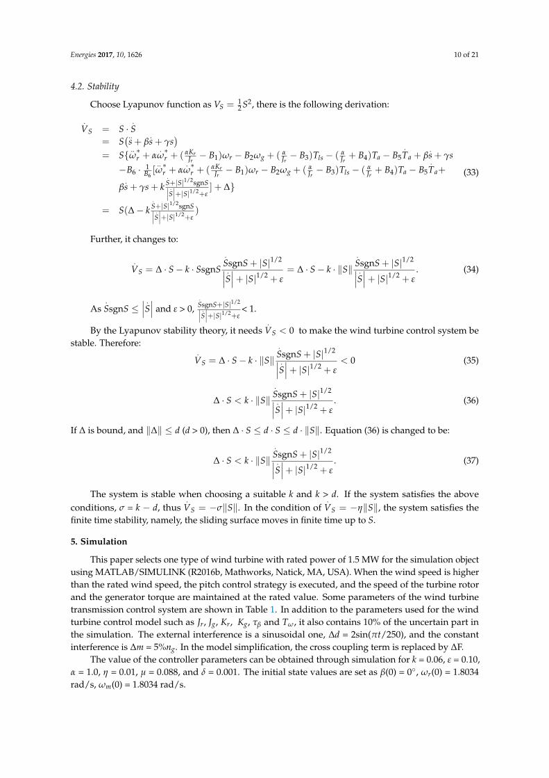
4.2. Stability

Choose Lyapunov function as VS = 12 S2, there is the following derivation:

.VS = S ·

.S

= S(..s + β

.s + γs

)= S ..

ω∗r + α

.ω∗r + ( αKr



Jr+ B4)Ta − B5

.Ta + β

.s + γs

−B6 · 1B6[

..ω∗r + α

.ω∗r + ( αKr



Jr+ B4)Ta − B5

.Ta+

β.s + γs + k

.S+|S|1/2sgnS∣∣∣ .S∣∣∣+|S|1/2+ε

] + ∆

= S(∆− k.S+|S|1/2sgnS∣∣∣ .S∣∣∣+|S|1/2+ε

)

(33)

Further, it changes to:

.VS = ∆ · S− k · SsgnS

.SsgnS + |S|1/2∣∣∣ .S∣∣∣+ |S|1/2 + ε

= ∆ · S− k · ‖S‖.SsgnS + |S|1/2∣∣∣ .S∣∣∣+ |S|1/2 + ε

. (34)

As.SsgnS ≤

∣∣∣ .S∣∣∣ and ε > 0,

.SsgnS+|S|1/2∣∣∣ .S∣∣∣+|S|1/2+ε

< 1.

By the Lyapunov stability theory, it needs.

VS < 0 to make the wind turbine control system bestable. Therefore:

.VS = ∆ · S− k · ‖S‖

.SsgnS + |S|1/2∣∣∣ .S∣∣∣+ |S|1/2 + ε

< 0 (35)

∆ · S < k · ‖S‖.SsgnS + |S|1/2∣∣∣ .S∣∣∣+ |S|1/2 + ε

. (36)

If ∆ is bound, and ‖∆‖ ≤ d (d > 0), then ∆ · S ≤ d · S ≤ d · ‖S‖. Equation (36) is changed to be:

∆ · S < k · ‖S‖.SsgnS + |S|1/2∣∣∣ .S∣∣∣+ |S|1/2 + ε

. (37)

The system is stable when choosing a suitable k and k > d. If the system satisfies the aboveconditions, σ = k − d, thus

.VS = −σ‖S‖. In the condition of

.VS = −η‖S‖, the system satisfies the

finite time stability, namely, the sliding surface moves in finite time up to S.

5. Simulation

This paper selects one type of wind turbine with rated power of 1.5 MW for the simulation objectusing MATLAB/SIMULINK (R2016b, Mathworks, Natick, MA, USA). When the wind speed is higherthan the rated wind speed, the pitch control strategy is executed, and the speed of the turbine rotorand the generator torque are maintained at the rated value. Some parameters of the wind turbinetransmission control system are shown in Table 1. In addition to the parameters used for the windturbine control model such as Jr, Jg, Kr, Kg, τβ and Tω, it also contains 10% of the uncertain part inthe simulation. The external interference is a sinusoidal one, ∆d = 2sin(πt/250), and the constantinterference is ∆m = 5%ng. In the model simplification, the cross coupling term is replaced by ∆F.

The value of the controller parameters can be obtained through simulation for k = 0.06, ε = 0.10,α = 1.0, η = 0.01, µ = 0.088, and δ = 0.001. The initial state values are set as β(0) = 0, ωr(0) = 1.8034rad/s, ωm(0) = 1.8034 rad/s.

Energies 2017, 10, 1626 11 of 21

Table 1. Related parameters of variable speed control system of wind turbines.

Parameter Name Symbol Numerical Unit

Turbine rotor radius R 38.5 mAir density ρ 1.225 kg/m3

Rated wind speed νrated 10.6 m/sRated turbine rotor speed ω∗rm 1.6755 rad/s

Rated power Perated 1.5 MWRated torque of generator Terated 8.74 kN ·m

Time constant of variable pitch actuator τβ 0.15Velocity actuator time constant Tω 0.05

Rotational inertia of rotor Jr 4.457× 106 kg ·m2

Rotational inertia of generator Jg 123 kg ·m2

Gearbox gear ratio ng 104Damping coefficient of turbine rotor Kr 45.52 N ·m/rad/s

Generator damping coefficient Kg 0.4 N ·m/rad/s

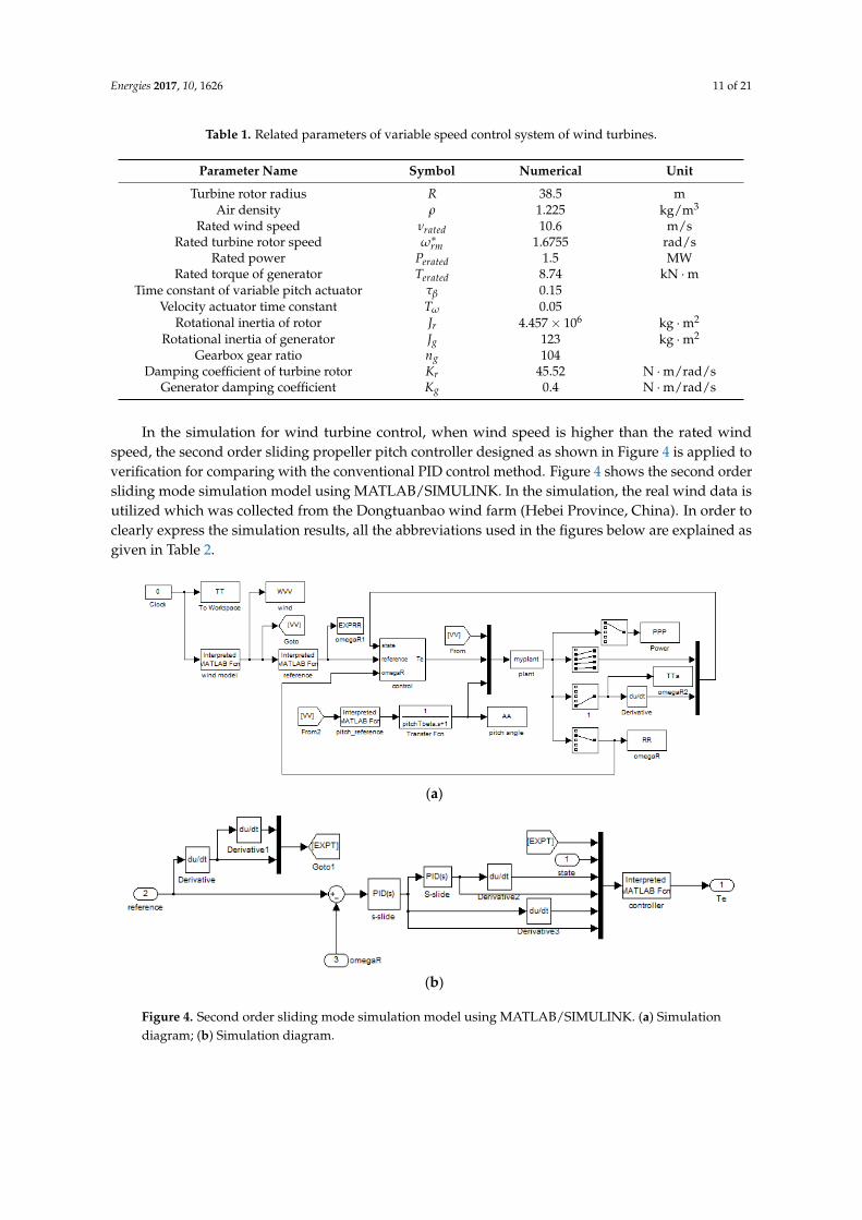
In the simulation for wind turbine control, when wind speed is higher than the rated windspeed, the second order sliding propeller pitch controller designed as shown in Figure 4 is applied toverification for comparing with the conventional PID control method. Figure 4 shows the second ordersliding mode simulation model using MATLAB/SIMULINK. In the simulation, the real wind data isutilized which was collected from the Dongtuanbao wind farm (Hebei Province, China). In order toclearly express the simulation results, all the abbreviations used in the figures below are explained asgiven in Table 2.

Energies 2017, 10, 1626 11 of 20

The value of the controller parameters can be obtained through simulation for k = 0.06, ε = 0.10, α = 1.0, η = 0.01, µ = 0.088, and δ = 0.001. The initial state values are set as β(0) = 0°, (0) = 1.8034 rad/s, (0) = 1.8034 rad/s.

Table 1. Related parameters of variable speed control system of wind turbines.

Parameter Name Symbol Numerical Unit Turbine rotor radius R 38.5 m

Air density ρ 1.225 3kg / m

Rated wind speed ratedν 10.6 m / s

Rated turbine rotor speed rmω∗ 1.6755 rad / s

Rated power eratedP 1.5 MW Rated torque of generator eratedT 8.74 kN m⋅

Time constant of variable pitch actuator βτ 0.15

Velocity actuator time constant Tω 0.05 Rotational inertia of rotor rJ

64.457 10× 2kg m⋅

Rotational inertia of generator gJ 123 2kg m⋅ Gearbox gear ratio gn 104

Damping coefficient of turbine rotor rK 45.52 N m / rad / s⋅ Generator damping coefficient gK 0.4 N m / rad / s⋅

In the simulation for wind turbine control, when wind speed is higher than the rated wind speed, the second order sliding propeller pitch controller designed as shown in Figure 4 is applied to verification for comparing with the conventional PID control method. Figure 4 shows the second order sliding mode simulation model using MATLAB/SIMULINK. In the simulation, the real wind data is utilized which was collected from the Dongtuanbao wind farm (Hebei Province, China). In order to clearly express the simulation results, all the abbreviations used in the figures below are explained as given in Table 2.

(a)

(b)

Figure 4. Second order sliding mode simulation model using MATLAB/SIMULINK. (a) Simulation diagram; (b) Simulation diagram. Figure 4. Second order sliding mode simulation model using MATLAB/SIMULINK. (a) Simulationdiagram; (b) Simulation diagram.

Energies 2017, 10, 1626 12 of 21

Table 2. Related abbreviations used in the figures.

Abbreviation Parameter Name

NEXPRR(rad/s) The expected rotor speedNRR(rad/s) Rotor speed using second order sliding mode controller

NRRPID(rad/s) Rotor speed using the PID controllerNRRTRA(rad/s) Rotor speed using the conventional sliding mode controllerNEEerror(rad/s) Rotor speed error using second order sliding mode controller to the expectation

NEEerrorPID(rad/s) Rotor speed error using the PID controller to the expectationNEEerrorTRA(rad/s) Rotor speed error using the conventional mode controller to the expectation

NPP(W) Output power using second order sliding mode controllerNPPPID(W) Output power using the PID controllerNPPTRA(W) Output power using the conventional sliding mode controllerNEXPPP(W) Output power calculated by the theoretical power curve

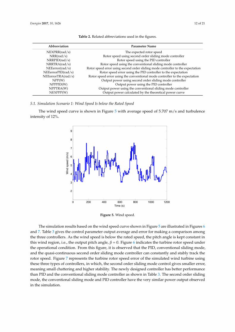
5.1. Simulation Scenario 1: Wind Speed Is below the Rated Speed

The wind speed curve is shown in Figure 5 with average speed of 5.707 m/s and turbulenceintensity of 12%.

Energies 2017, 10, 1626 12 of 20

Table 2. Related abbreviations used in the figures.

Abbreviation Parameter Name

NEXPRR(rad/s) The expected rotor speed NRR(rad/s) Rotor speed using second order sliding mode controller

NRRPID(rad/s) Rotor speed using the PID controller NRRTRA(rad/s) Rotor speed using the conventional sliding mode controller NEEerror(rad/s) Rotor speed error using second order sliding mode controller to the expectation

NEEerrorPID(rad/s) Rotor speed error using the PID controller to the expectation NEEerrorTRA(rad/s) Rotor speed error using the conventional mode controller to the expectation

NPP(W) Output power using second order sliding mode controller NPPPID(W) Output power using the PID controller NPPTRA(W) Output power using the conventional sliding mode controller NEXPPP(W) Output power calculated by the theoretical power curve

5.1. Simulation Scenario 1: Wind Speed Is below the Rated Speed

The wind speed curve is shown in Figure 5 with average speed of 5.707 m/s and turbulence intensity of 12%.

Figure 5. Wind speed.

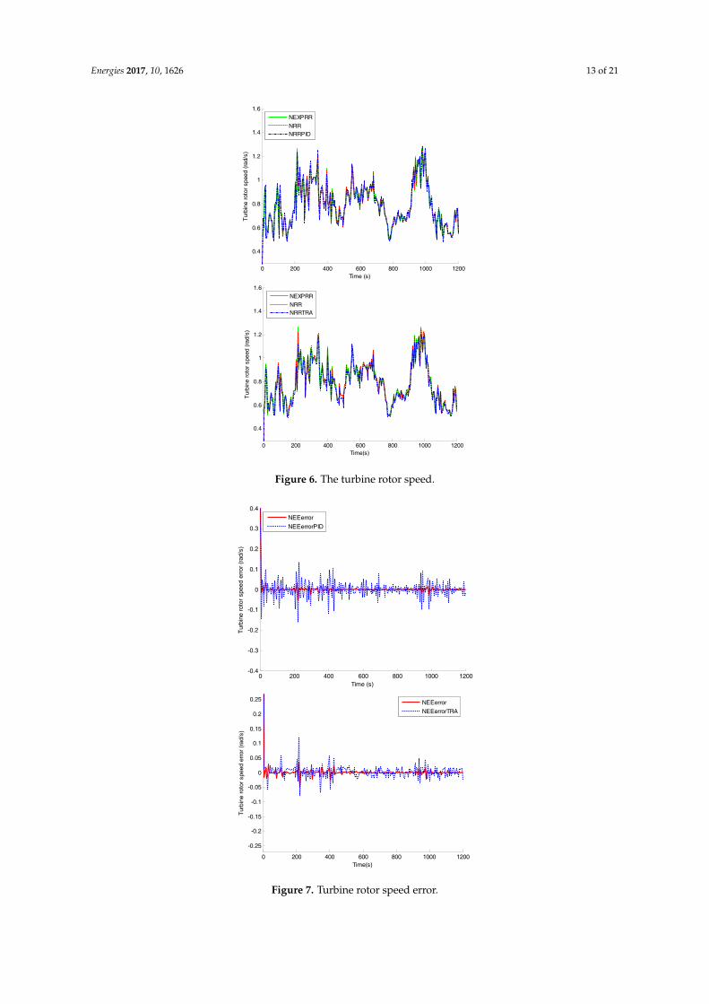
The simulation results based on the wind speed curve shown in Figure 5 are illustrated in Figures 6 and 7. Table 3 gives the control parameter output average and error for making a comparison among the three controllers. As the wind speed is below the rated speed, the pitch angle is kept constant in this wind region, i.e., the output pitch angle, β = 0. Figure 6 indicates the turbine rotor speed under the operational condition. From this figure, it is observed that the PID, conventional sliding mode, and the quasi-continuous second order sliding mode controller can constantly and stably track the rotor speed. Figure 7 represents the turbine rotor speed error of the simulated wind turbine using these three types of controllers, in which, the second order sliding mode control gives smaller error, meaning small chattering and higher stability. The newly designed controller has better performance than PID and the conventional sliding mode controller as shown in Table 3. The second order sliding mode, the conventional sliding mode and PID controller have the very similar power output observed in the simulation.

0 200 400 600 800 1000 1200

2

3

4

5

6

7

8

9

Time (s)

Win

d sp

eed

(m/s

)


The simulation results based on the wind speed curve shown in Figure 5 are illustrated in Figures 6and 7. Table 3 gives the control parameter output average and error for making a comparison amongthe three controllers. As the wind speed is below the rated speed, the pitch angle is kept constant inthis wind region, i.e., the output pitch angle, β = 0. Figure 6 indicates the turbine rotor speed underthe operational condition. From this figure, it is observed that the PID, conventional sliding mode,and the quasi-continuous second order sliding mode controller can constantly and stably track therotor speed. Figure 7 represents the turbine rotor speed error of the simulated wind turbine usingthese three types of controllers, in which, the second order sliding mode control gives smaller error,meaning small chattering and higher stability. The newly designed controller has better performancethan PID and the conventional sliding mode controller as shown in Table 3. The second order slidingmode, the conventional sliding mode and PID controller have the very similar power output observedin the simulation.

Energies 2017, 10, 1626 13 of 21Energies 2017, 10, 1626 13 of 20

Figure 6. The turbine rotor speed.

Figure 7. Turbine rotor speed error.

0 200 400 600 800 1000 1200

0.4

0.6

0.8

1

1.2

1.4

1.6

Time (s)

Turb

ine

roto

r sp

eed

(rad/

s)

NEXPRRNRRNRRPID

0 200 400 600 800 1000 1200

0.4

0.6

0.8

1

1.2

1.4

1.6

Time(s)

Tur

bine

rot

or s

peed

(ra

d/s)

NEXPRRNRRNRRTRA

0 200 400 600 800 1000 1200-0.4

-0.3

-0.2

-0.1

0

0.1

0.2

0.3

0.4

Time (s)

Turb

ine

roto

r sp

eed

erro

r (ra

d/s)

NEEerrorNEEerrorPID

0 200 400 600 800 1000 1200

-0.25

-0.2

-0.15

-0.1

-0.05

0

0.05

0.1

0.15

0.2

0.25

Time(s)

Turb

ine

roto

r sp

eed

erro

r (ra

d/s)

NEEerrorNEEerrorTRA


Energies 2017, 10, 1626 13 of 20



0 200 400 600 800 1000 1200

0.4

0.6

0.8

1

1.2

1.4

1.6

Time (s)

Turb

ine

roto

r sp

eed

(rad/

s)

NEXPRRNRRNRRPID

0 200 400 600 800 1000 1200

0.4

0.6

0.8

1

1.2

1.4

1.6

Time(s)

Tur

bine

rot

or s

peed

(ra

d/s)

NEXPRRNRRNRRTRA

0 200 400 600 800 1000 1200-0.4

-0.3

-0.2

-0.1

0

0.1

0.2

0.3

0.4

Time (s)

Turb

ine

roto

r sp

eed

erro

r (ra

d/s)

NEEerrorNEEerrorPID

0 200 400 600 800 1000 1200

-0.25

-0.2

-0.15

-0.1

-0.05

0

0.05

0.1

0.15

0.2

0.25

Time(s)

Turb

ine

roto

r sp

eed

erro

r (ra

d/s)

NEEerrorNEEerrorTRA


Energies 2017, 10, 1626 14 of 21

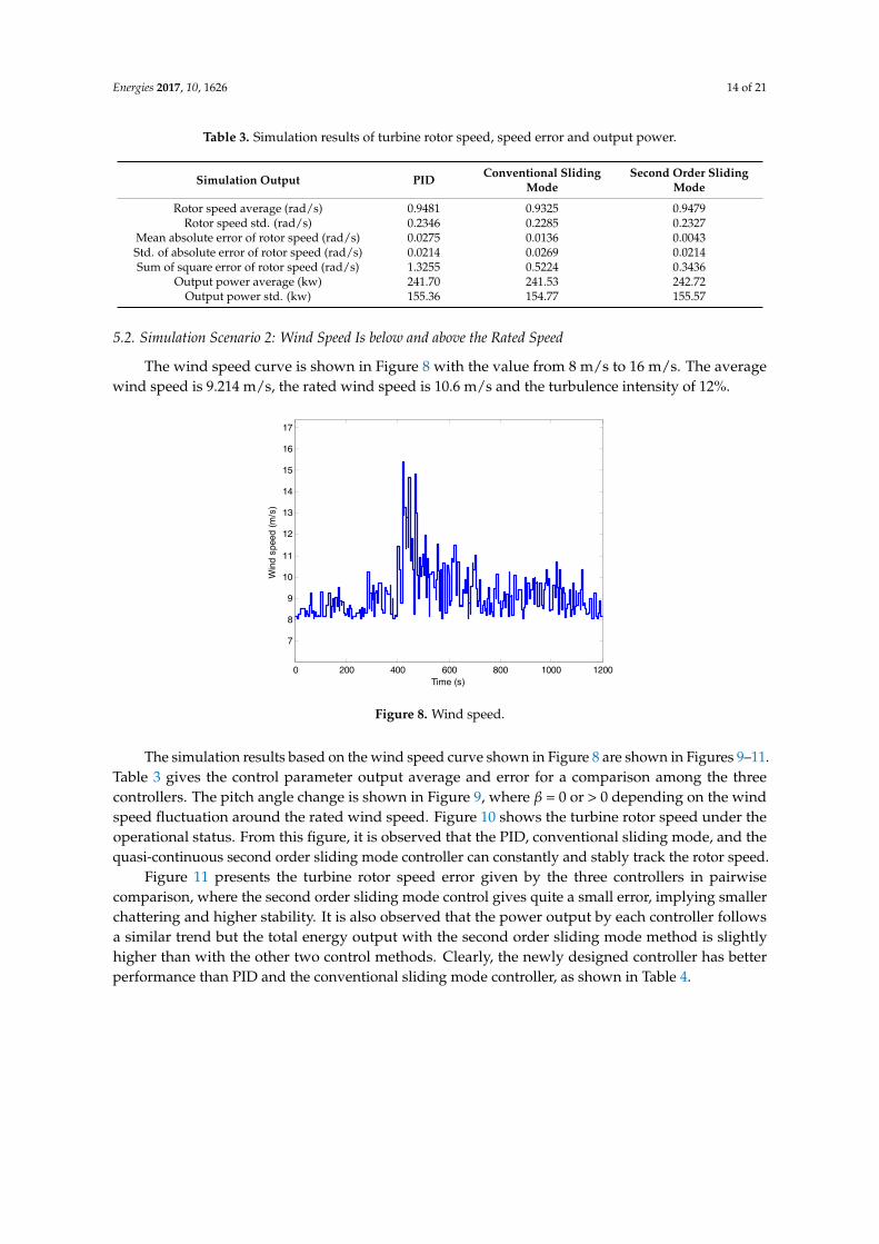
Table 3. Simulation results of turbine rotor speed, speed error and output power.

Simulation Output PID Conventional SlidingMode

Second Order SlidingMode

Rotor speed average (rad/s) 0.9481 0.9325 0.9479Rotor speed std. (rad/s) 0.2346 0.2285 0.2327

Mean absolute error of rotor speed (rad/s) 0.0275 0.0136 0.0043Std. of absolute error of rotor speed (rad/s) 0.0214 0.0269 0.0214Sum of square error of rotor speed (rad/s) 1.3255 0.5224 0.3436

Output power average (kw) 241.70 241.53 242.72Output power std. (kw) 155.36 154.77 155.57

5.2. Simulation Scenario 2: Wind Speed Is below and above the Rated Speed

The wind speed curve is shown in Figure 8 with the value from 8 m/s to 16 m/s. The averagewind speed is 9.214 m/s, the rated wind speed is 10.6 m/s and the turbulence intensity of 12%.

Energies 2017, 10, 1626 14 of 20


Simulation Output PID Conventional Sliding

Mode Second Order Sliding

Mode Rotor speed average (rad/s) 0.9481 0.9325 0.9479

Rotor speed std. (rad/s) 0.2346 0.2285 0.2327 Mean absolute error of rotor speed (rad/s) 0.0275 0.0136 0.0043 Std. of absolute error of rotor speed (rad/s) 0.0214 0.0269 0.0214 Sum of square error of rotor speed (rad/s) 1.3255 0.5224 0.3436

Output power average (kw) 241.70 241.53 242.72 Output power std. (kw) 155.36 154.77 155.57


The wind speed curve is shown in Figure 8 with the value from 8 m/s to 16 m/s. The average wind speed is 9.214 m/s, the rated wind speed is 10.6 m/s and the turbulence intensity of 12%.


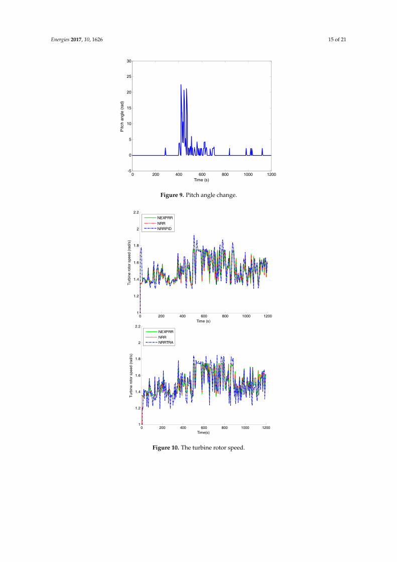
The simulation results based on the wind speed curve shown in Figure 8 are shown in Figures 9–11. Table 3 gives the control parameter output average and error for a comparison among the three controllers. The pitch angle change is shown in Figure 9, where β = 0 or > 0 depending on the wind speed fluctuation around the rated wind speed. Figure 10 shows the turbine rotor speed under the operational status. From this figure, it is observed that the PID, conventional sliding mode, and the quasi-continuous second order sliding mode controller can constantly and stably track the rotor speed.

Figure 9. Pitch angle change.

0 200 400 600 800 1000 1200

7

8

9

10

11

12

13

14

15

16

17

Time (s)

Win

d sp

eed

(m/s

)

0 200 400 600 800 1000 1200-5

0

5

10

15

20

25

30

Time (s)

Pitc

h an

gle

(rad

)


The simulation results based on the wind speed curve shown in Figure 8 are shown in Figures 9–11.Table 3 gives the control parameter output average and error for a comparison among the threecontrollers. The pitch angle change is shown in Figure 9, where β = 0 or > 0 depending on the windspeed fluctuation around the rated wind speed. Figure 10 shows the turbine rotor speed under theoperational status. From this figure, it is observed that the PID, conventional sliding mode, and thequasi-continuous second order sliding mode controller can constantly and stably track the rotor speed.

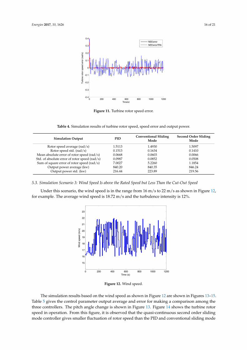
Figure 11 presents the turbine rotor speed error given by the three controllers in pairwisecomparison, where the second order sliding mode control gives quite a small error, implying smallerchattering and higher stability. It is also observed that the power output by each controller followsa similar trend but the total energy output with the second order sliding mode method is slightlyhigher than with the other two control methods. Clearly, the newly designed controller has betterperformance than PID and the conventional sliding mode controller, as shown in Table 4.

Energies 2017, 10, 1626 15 of 21

Energies 2017, 10, 1626 14 of 20


Simulation Output PID Conventional Sliding

Mode Second Order Sliding

Mode Rotor speed average (rad/s) 0.9481 0.9325 0.9479




The wind speed curve is shown in Figure 8 with the value from 8 m/s to 16 m/s. The average wind speed is 9.214 m/s, the rated wind speed is 10.6 m/s and the turbulence intensity of 12%.


The simulation results based on the wind speed curve shown in Figure 8 are shown in Figures 9–11. Table 3 gives the control parameter output average and error for a comparison among the three controllers. The pitch angle change is shown in Figure 9, where β = 0 or > 0 depending on the wind speed fluctuation around the rated wind speed. Figure 10 shows the turbine rotor speed under the operational status. From this figure, it is observed that the PID, conventional sliding mode, and the quasi-continuous second order sliding mode controller can constantly and stably track the rotor speed.


0 200 400 600 800 1000 1200

7

8

9

10

11

12

13

14

15

16

17

Time (s)

Win

d sp

eed

(m/s

)

0 200 400 600 800 1000 1200-5

0

5

10

15

20

25

30

Time (s)

Pitc

h an

gle

(rad

)

Figure 9. Pitch angle change.Energies 2017, 10, 1626 15 of 20



Figure 11 presents the turbine rotor speed error given by the three controllers in pairwise comparison, where the second order sliding mode control gives quite a small error, implying smaller chattering and higher stability. It is also observed that the power output by each controller follows a similar trend but the total energy output with the second order sliding mode method is slightly higher than with the other two control methods. Clearly, the newly designed controller has better performance than PID and the conventional sliding mode controller, as shown in Table 4.


Simulation Output PID Conventional Sliding Mode Second Order Sliding ModeRotor speed average (rad/s) 1.5113 1.4930 1.5097


0 200 400 600 800 1000 12001

1.2

1.4

1.6

1.8

2

2.2

Time (s)

Tur

bine

rot

or s

peed

(ra

d/s)

NEXPRRNRRNRRPID

0 200 400 600 800 1000 12001

1.2

1.4

1.6

1.8

2

2.2

Time(s)

Turb

ine

roto

r sp

eed

(rad/

s)

NEXPRRNRRNRRTRA

0 200 400 600 800 1000 1200-0.4

-0.3

-0.2

-0.1

0

0.1

0.2

0.3

0.4

Time(s)

Turb

ine

roto

r spe

ed e

rror

(ra

d/s)

NEEerrorNEEerrorTRA


Energies 2017, 10, 1626 16 of 21

Energies 2017, 10, 1626 15 of 20



Figure 11 presents the turbine rotor speed error given by the three controllers in pairwise comparison, where the second order sliding mode control gives quite a small error, implying smaller chattering and higher stability. It is also observed that the power output by each controller follows a similar trend but the total energy output with the second order sliding mode method is slightly higher than with the other two control methods. Clearly, the newly designed controller has better performance than PID and the conventional sliding mode controller, as shown in Table 4.




0 200 400 600 800 1000 12001

1.2

1.4

1.6

1.8

2

2.2

Time (s)

Tur

bine

rot

or s

peed

(ra

d/s)

NEXPRRNRRNRRPID

0 200 400 600 800 1000 12001

1.2

1.4

1.6

1.8

2

2.2

Time(s)

Turb

ine

roto

r sp

eed

(rad/

s)

NEXPRRNRRNRRTRA

0 200 400 600 800 1000 1200-0.4

-0.3

-0.2

-0.1

0

0.1

0.2

0.3

0.4

Time(s)

Turb

ine

roto

r spe

ed e

rror

(ra

d/s)

NEEerrorNEEerrorTRA



Simulation Output PID Conventional SlidingMode

Second Order SlidingMode




5.3. Simulation Scenario 3: Wind Speed Is above the Rated Speed but Less Than the Cut-Out Speed

Under this scenario, the wind speed is in the range from 16 m/s to 22 m/s as shown in Figure 12,for example. The average wind speed is 18.72 m/s and the turbulence intensity is 12%.

Energies 2017, 10, 1626 16 of 20



Under this scenario, the wind speed is in the range from 16 m/s to 22 m/s as shown in Figure 12, for example. The average wind speed is 18.72 m/s and the turbulence intensity is 12%.


The simulation results based on the wind speed as shown in Figure 12 are shown in Figures 13–15. Table 5 gives the control parameter output average and error for making a comparison among the three controllers. The pitch angle change is shown in Figure 13. Figure 14 shows the turbine rotor speed in operation. From this figure, it is observed that the quasi-continuous second order sliding mode controller gives smaller fluctuation of rotor speed than the PID and conventional sliding mode controller. It is clearly shown that the turbine rotor speed error given by the sliding mode controllers is much smaller than the PID controller. That means small chattering and higher stability can be achieved by the second order sliding mode control method.


0 200 400 600 800 1000 1200

15

16

17

18

19

20

21

22

23

Time (s)

Win

d sp

eed

(m/s

)

0 200 400 600 800 1000 120020

22

24

26

28

30

32

34

36

38

40

Time (s)

Pitc

h an

gle

(rad

)


The simulation results based on the wind speed as shown in Figure 12 are shown in Figures 13–15.Table 5 gives the control parameter output average and error for making a comparison among thethree controllers. The pitch angle change is shown in Figure 13. Figure 14 shows the turbine rotorspeed in operation. From this figure, it is observed that the quasi-continuous second order slidingmode controller gives smaller fluctuation of rotor speed than the PID and conventional sliding mode

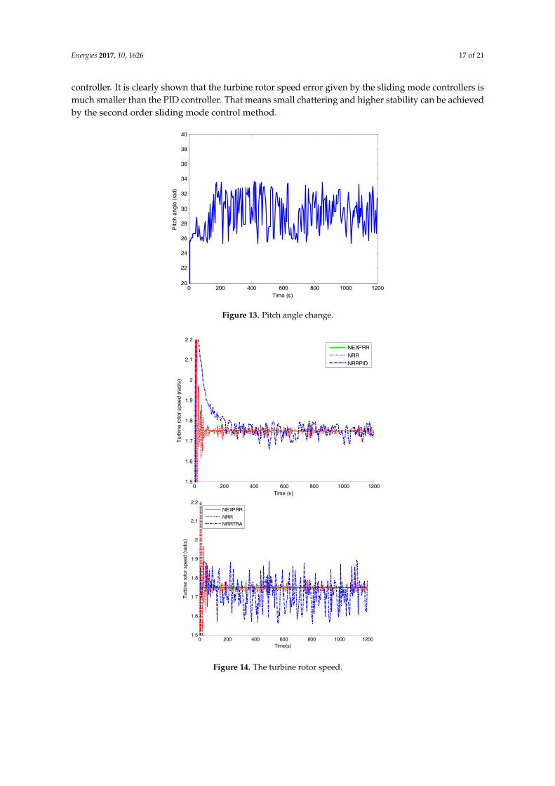
Energies 2017, 10, 1626 17 of 21

controller. It is clearly shown that the turbine rotor speed error given by the sliding mode controllers ismuch smaller than the PID controller. That means small chattering and higher stability can be achievedby the second order sliding mode control method.

Energies 2017, 10, 1626 16 of 20



Under this scenario, the wind speed is in the range from 16 m/s to 22 m/s as shown in Figure 12, for example. The average wind speed is 18.72 m/s and the turbulence intensity is 12%.


The simulation results based on the wind speed as shown in Figure 12 are shown in Figures 13–15. Table 5 gives the control parameter output average and error for making a comparison among the three controllers. The pitch angle change is shown in Figure 13. Figure 14 shows the turbine rotor speed in operation. From this figure, it is observed that the quasi-continuous second order sliding mode controller gives smaller fluctuation of rotor speed than the PID and conventional sliding mode controller. It is clearly shown that the turbine rotor speed error given by the sliding mode controllers is much smaller than the PID controller. That means small chattering and higher stability can be achieved by the second order sliding mode control method.


0 200 400 600 800 1000 1200

15

16

17

18

19

20

21

22

23

Time (s)

Win

d sp

eed

(m/s

)

0 200 400 600 800 1000 120020

22

24

26

28

30

32

34

36

38

40

Time (s)

Pitc

h an

gle

(rad

)

Figure 13. Pitch angle change.Energies 2017, 10, 1626 17 of 20


0 200 400 600 800 1000 12001.5

1.6

1.7

1.8

1.9

2

2.1

2.2

Time (s)

Tur

bine

roto

r sp

eed

(rad

/s)

NEXPRRNRRNRRPID

0 200 400 600 800 1000 12001.5

1.6

1.7

1.8

1.9

2

2.1

2.2

Time(s)

Tur

bine

rot

or s

peed

(ra

d/s)

NEXPRRNRRNRRTRA

0 200 400 600 800 1000 1200800

900

1000

1100

1200

1300

1400

1500

1600

1700

1800

Time (s)

Pow

er (

kW)

NPPPIDNEXPPP

0 200 400 600 800 1000 1200900

1000

1100

1200

1300

1400

1500

1600

1700

1800

1900

2000

Time (s)

Pow

er (

kW)

NPPTRANEXPPP


Energies 2017, 10, 1626 18 of 21

Energies 2017, 10, 1626 17 of 20


0 200 400 600 800 1000 12001.5

1.6

1.7

1.8

1.9

2

2.1

2.2

Time (s)

Tur

bine

roto

r sp

eed

(rad

/s)

NEXPRRNRRNRRPID

0 200 400 600 800 1000 12001.5

1.6

1.7

1.8

1.9

2

2.1

2.2

Time(s)

Tur

bine

rot

or s

peed

(ra

d/s)

NEXPRRNRRNRRTRA

0 200 400 600 800 1000 1200800

900

1000

1100

1200

1300

1400

1500

1600

1700

1800

Time (s)

Pow

er (

kW)

NPPPIDNEXPPP

0 200 400 600 800 1000 1200900

1000

1100

1200

1300

1400

1500

1600

1700

1800

1900

2000

Time (s)

Pow

er (

kW)

NPPTRANEXPPP

Energies 2017, 10, 1626 18 of 20

Figure 15. Output power.





Figure 15 presents the simulated output power using the three controllers. It demonstrates that the quasi-continuous second order sliding mode controller gives smaller fluctuation of out power than the PID and conventional sliding mode controller. Clearly, the newly designed controller has better performance than PID and the conventional sliding mode controller as shown in Table 5.

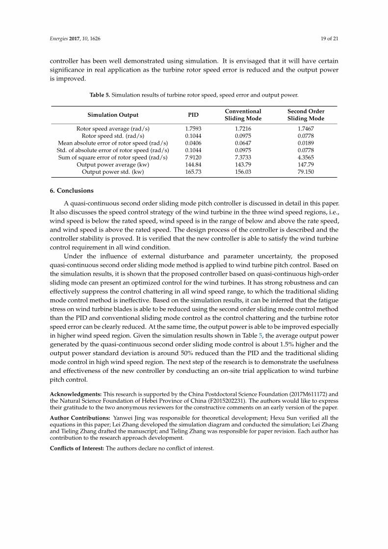
In summary, the proposed quasi-continuous second order sliding mode pitch controller has strong robustness under the influence of disturbance and model parameter uncertainty. It can effectively reduce buffeting and the mechanical stress of the system. The effectiveness of the newly designed controller has been well demonstrated using simulation. It is envisaged that it will have certain significance in real application as the turbine rotor speed error is reduced and the output power is improved.

6. Conclusions

A quasi-continuous second order sliding mode pitch controller is discussed in detail in this paper. It also discusses the speed control strategy of the wind turbine in the three wind speed regions, i.e., wind speed is below the rated speed, wind speed is in the range of below and above the rate speed, and wind speed is above the rated speed. The design process of the controller is described and the controller stability is proved. It is verified that the new controller is able to satisfy the wind turbine control requirement in all wind condition.

Under the influence of external disturbance and parameter uncertainty, the proposed quasi-continuous second order sliding mode method is applied to wind turbine pitch control. Based on the simulation results, it is shown that the proposed controller based on quasi-continuous high-order sliding mode can present an optimized control for the wind turbines. It has strong robustness and can effectively suppress the control chattering in all wind speed range, to which the traditional sliding mode control method is ineffective. Based on the simulation results, it can be inferred that the fatigue stress on wind turbine blades is able to be reduced using the second order sliding mode control method than the PID and conventional sliding mode control as the control chattering and the turbine rotor speed error can be clearly reduced. At the same time, the output power is able to be improved especially in higher wind speed region. Given the simulation results shown in Table 5, the average output power generated by the quasi-continuous second order

0 200 400 600 800 1000 1200900

1000

1100

1200

1300

1400

1500

1600

1700

1800

Time (s)

Pow

er (k

W)

NPPNEXPPP

Figure 15. Output power.

Figure 15 presents the simulated output power using the three controllers. It demonstrates thatthe quasi-continuous second order sliding mode controller gives smaller fluctuation of out power thanthe PID and conventional sliding mode controller. Clearly, the newly designed controller has betterperformance than PID and the conventional sliding mode controller as shown in Table 5.

In summary, the proposed quasi-continuous second order sliding mode pitch controller has strongrobustness under the influence of disturbance and model parameter uncertainty. It can effectivelyreduce buffeting and the mechanical stress of the system. The effectiveness of the newly designed

Energies 2017, 10, 1626 19 of 21

controller has been well demonstrated using simulation. It is envisaged that it will have certainsignificance in real application as the turbine rotor speed error is reduced and the output poweris improved.


Simulation Output PID ConventionalSliding Mode

Second OrderSliding Mode




6. Conclusions

A quasi-continuous second order sliding mode pitch controller is discussed in detail in this paper.It also discusses the speed control strategy of the wind turbine in the three wind speed regions, i.e.,wind speed is below the rated speed, wind speed is in the range of below and above the rate speed,and wind speed is above the rated speed. The design process of the controller is described and thecontroller stability is proved. It is verified that the new controller is able to satisfy the wind turbinecontrol requirement in all wind condition.

Under the influence of external disturbance and parameter uncertainty, the proposedquasi-continuous second order sliding mode method is applied to wind turbine pitch control. Based onthe simulation results, it is shown that the proposed controller based on quasi-continuous high-ordersliding mode can present an optimized control for the wind turbines. It has strong robustness and caneffectively suppress the control chattering in all wind speed range, to which the traditional slidingmode control method is ineffective. Based on the simulation results, it can be inferred that the fatiguestress on wind turbine blades is able to be reduced using the second order sliding mode control methodthan the PID and conventional sliding mode control as the control chattering and the turbine rotorspeed error can be clearly reduced. At the same time, the output power is able to be improved especiallyin higher wind speed region. Given the simulation results shown in Table 5, the average output powergenerated by the quasi-continuous second order sliding mode control is about 1.5% higher and theoutput power standard deviation is around 50% reduced than the PID and the traditional slidingmode control in high wind speed region. The next step of the research is to demonstrate the usefulnessand effectiveness of the new controller by conducting an on-site trial application to wind turbinepitch control.

Acknowledgments: This research is supported by the China Postdoctoral Science Foundation (2017M611172) andthe Natural Science Foundation of Hebei Province of China (F2015202231). The authors would like to expresstheir gratitude to the two anonymous reviewers for the constructive comments on an early version of the paper.

Author Contributions: Yanwei Jing was responsible for theoretical development; Hexu Sun verified all theequations in this paper; Lei Zhang developed the simulation diagram and conducted the simulation; Lei Zhangand Tieling Zhang drafted the manuscript; and Tieling Zhang was responsible for paper revision. Each author hascontribution to the research approach development.

Conflicts of Interest: The authors declare no conflict of interest.

Energies 2017, 10, 1626 20 of 21

Acronyms and Nomenclature

MPPT Maximum power point tracking Jg Generator inertia (kg·m2)TSR Blade tip speed ratio ng Gearbox ratioPa Mechanical power (W) Tls The low speed shaft torque (N·m)v Wind speed (m/s) Ueq Equivalent control quantityρ Air density (kg/m3) US Switching control quantityR Wind turbine rotor radius (m) Jr Rotor moment of inertia (kg·m2)λ Tip speed ratio ωg Generator speed (rad/s)β The actual output pitch angle () Kr The damping coefficient of turbineCp(λ, β) Turbine power conversion efficiency rotor (N·m/rad/s)g The number of pairs of poles Kg Generator external damping coefficientTa Aerodynamic torque (N·m) (N·m/rad/s)Te Generator torque (N·m) Kls The low speed shaft damping (N·m/rad/s)Ths Input torque to generator (N·m) Bls The low speed shaft stiffness (N·m/rad)ωr Turbine rotor speed (rad/s) β∗ The reference value of the pitch angle ()ωls The low speed shaft speed (rad/s) C1 Correction factorω1 Generator synchronous speed (rad/s) m1 Relative numberr1 Stator winding resistance (Ω) U1 Network voltage (V)x1 Stator winding leakage reactance (Ω) vcut-in Cut-in wind speed (m/s)r2′ Rotor winding resistance (Ω) vrmax The wind speed where ωr reaches thex2′ Rotor winding leakage reactance (Ω) rated rotational speed (m/s)τβ Time constant vrated The rated wind speed (m/s)

vcut-off Cut-off wind speed (m/s)

References

1. Torchani, B.; Sellami, A.; Garcia, G. Saturateci sliding mode control for variable speed wind turbine.In Proceedings of the 5th International Renewable Energy Congress (IREC), Hammamet, Tunisia, 25–27March 2014; pp. 1–5.

2. Liu, X.; Han, Y.; Wang, C. Second-order sliding mode control for power optimization of DFIG-based variablespeed wind turbine. IET Renew. Power Gener. 2017, 11, 408–418. [CrossRef]

3. Jafarnejadsani, H.; Pieper, J.; Ehlers, J. Adaptive control of a variable-speed variable-pitch wind turbineusing radial-basis function neural network. IEEE Trans. Control Syst. Technol. 2013, 21, 2264–2272. [CrossRef]

4. Zhang, B.M.; Chen, J.H.; Wu, W.C. A Hierarchical model predictive control method of active power foraccommodating large-scale wind power integration. Autom. Electr. Power Syst. 2014, 09, 6–14.

5. Evangelista, C.; Valenciaga, F.; Puleston, P. Active and reactive power control for wind turbine based ona MIMO 2-sliding mode algorithm with variable gains. IEEE Trans. Energy Convers. 2013, 28, 682–689.[CrossRef]

6. Xie, J.P. Study on Maximal Wind Energy Capture and Grid Connection of Wind Generator System; YanshanUniversity: Qinhuangdao, China, 2013.

7. Boukhezzar, B.; Lupu, L.; Siguerdidjanea, H.; Hand, M. Multivariable control strategy for variable speed,variable pitch wind turbines. Renew. Energy 2007, 32, 1273–1287. [CrossRef]

8. Van Baars, G.E.; Bongers, P.M. Wind turbine control design and implementation based on experimentalmodels. In Proceedings of the 31st Conference on Decision and Control, Tucson, AZ, USA, 16–18 December1992; pp. 2596–2600.

9. Zinger, D.S.; Muljadi, E.; Miller, A. A simple control scheme for variable speed wind turbines. In Proceedingsof the Conference Record of the 1996 IEEE Industry Applications Conference Thirty-First IAS AnnualMeeting, San Diego, CA, USA, 6–10 October 1996; pp. 1613–1618.

10. Hand, M. Variable-Speed Wind Turbine Controller Systematic Designs Methodology: A Comparison of Nonlinear andLinear Model-Based Designs; NREL Report TP-500e25540; National Renewable Energy Laboratory: Golden,CO, USA, 1999.

11. Moradi, H.; Vossoughi, G. Robust control of the variable speed wind turbines in the presence of uncertainties:A comparison between H-infinity and PID controllers. Energy 2015, 90, 1508–1521. [CrossRef]

http://dx.doi.org/10.1049/iet-rpg.2015.0403

http://dx.doi.org/10.1109/TCST.2012.2237518

http://dx.doi.org/10.1109/TEC.2013.2272244

http://dx.doi.org/10.1016/j.renene.2006.06.010

http://dx.doi.org/10.1016/j.energy.2015.06.100

Energies 2017, 10, 1626 21 of 21

12. Pieralli, S.; Ritter, M.; Odening, M. Efficiency of wind power production and its determinants. Energy 2015,90, 429–438. [CrossRef]

13. Taveiros, F.E.V.; Barros, L.S.; Costa, F.B. Back-to-back converter state-feedback control of DFIG (doubly-fedinduction generator)-based wind turbines. Energy 2015, 89, 896–906. [CrossRef]

14. Zong, Q.; Wang, J.; Tian, B.L.; Tao, Y. Quasi-continuous high-order sliding mode controller and observerdesign for flexible hypersonic vehicle. Aerosp. Sci. Technol. 2013, 27, 127–137. [CrossRef]

15. Saravanakumar, R.; Jena, D. Validation of an integral sliding mode control for optimal control of a threeblade variable speed variable pitch wind turbine. Electr. Power Energy Syst. 2015, 69, 421–429. [CrossRef]

16. Evangelista, C.; Puleston, P.; Valenciaga, F.; Fridman, L.M. Lyapunov-designed super-twisting sliding modecontrol for wind energy conversion optimization. IEEE Trans. Ind. Electron. 2013, 60, 538–545. [CrossRef]

17. Beltran, B.; Tarek, A.; Benbouzid, M. Sliding mode power control of variable-speed wind energy conversionsystems. IEEE Trans. Energy Convers. 2008, 23, 551–588. [CrossRef]

18. Beltran, B.; Tarek, A.; Benbouzid, M. High-order sliding mode control of variable-speed wind turbines.IEEE Trans. Ind. Electron. 2009, 56, 3314–3321. [CrossRef]

19. Merida, J.; Aguilar, L.T.; Davila, J. Analysis and synthesis of sliding mode control for large scale variablespeed wind turbine for power optimization. Renew. Energy 2014, 71, 715–728. [CrossRef]

20. Zinober, A.S.I. (Ed.) Deterministic Control of Uncertain Systems; Peter Peregrinus Press: London, UK, 1990;ISBN 978-0-86341-170-0.

21. Qin, B.; Zhou, H.; Du, K.; Wang, X. Sliding mode control of pitch angle based on RBF neural-network.Trans. China Electrotech. Soc. 2013, 28, 37–41.

22. Levant, A. High-order sliding modes, differentiation and output- feedback control. Int. J. Control 2003, 76,924–941. [CrossRef]

23. Levant, A. Quasi-continuous high-order sliding-mode controllers. IEEE Trans. Autom. Control 2005, 50,1812–1815. [CrossRef]

24. Hu, Y. The Application of Quasi-continuous High Order Sliding Mode in the Controller Design of Hypersonic Vehicles;Huazhong University of Science and Technology: Wuhan, China, 2012.

25. Levant, A. Homogeneity approach to high-order sliding mode design. Automatica 2005, 41, 823–830.[CrossRef]

26. Zhao, W.W.; Zhang, L.; Jing, Y.W. Optimization design of controller for pitch wind turbine. Power Syst.Technol. 2014, 12, 3436–3440.

27. Abdeddaim, S.; Betka, A. Optimal tracking and robust power control of the DFIG wind turbine. Electr. PowerEnergy Syst. 2013, 49, 234–242. [CrossRef]

28. Saravanakumar, R.; Jena, D. A novel fuzzy integral sliding mode current control strategy for maximizingwind power extraction and eliminating voltage harmonics. Energy 2015, 85, 677–686.

29. Zhou, Z.C.; Wang, C.S.; Guo, L. Output power curtailment control of variable-speed variable-pitch windturbine generator at all wind speed regions. Proc. CSEE 2005, 35, 1837–1844.

30. Wang, J.; Zong, Q.; Tian, B.L.; Fan, W.R. Reentry attitude control for hypersonic vehicle based onquasi-continuous high order sliding mode. Control Theory Appl. 2014, 31, 1166–1173.

© 2017 by the authors. Licensee MDPI, Basel, Switzerland. This article is an open accessarticle distributed under the terms and conditions of the Creative Commons Attribution(CC BY) license (http://creativecommons.org/licenses/by/4.0/).



http://dx.doi.org/10.1016/j.ast.2012.07.004

http://dx.doi.org/10.1016/j.ijepes.2015.01.031

http://dx.doi.org/10.1109/TIE.2012.2188256

http://dx.doi.org/10.1109/TEC.2007.914163

http://dx.doi.org/10.1109/TIE.2008.2006949

http://dx.doi.org/10.1016/j.renene.2014.06.030

http://dx.doi.org/10.1080/0020717031000099029

http://dx.doi.org/10.1109/TAC.2005.858646

http://dx.doi.org/10.1016/j.automatica.2004.11.029

http://dx.doi.org/10.1016/j.ijepes.2012.12.014

http://creativecommons.org/

http://creativecommons.org/licenses/by/4.0/.

Documents

Variable Speed Control of Wind Turbines Based on the Quasi ... filecoupling, as well as external interference, present great challenges in wind turbine controller design. In this paper,