VARIABLE SELECTION

IN FINITE MIXTURE OF REGRESSION MODELS

Abbas Khalili and Jiahua Chen 1

Department of Statistics and Actuarial Science, University of Waterloo

Abstract: In the applications of finite mixture of regression models, a large number

of covariates are often used and their contributions toward the response variable vary

from one component to another of the mixture model. This creates a complex vari-

able selection problem. Existing methods, such as AIC and BIC, are computationally

expensive as the number of covariates and the components in the mixture model

increase. In this paper, we introduce a penalized likelihood approach for variable se-

lection in finite mixture of regression models. The new method introduces a penalty

which depends on the sizes of regression coefficients and the mixture structure. The

new method is shown to have the desired sparsity property. A data adaptive method

for selecting tuning parameters, and an EM-algorithm for efficient numerical compu-

tations are developed. Simulations show that the method has very good performance

with much lower demand on computing power. The new method is also illustrated

by analyzing a real data set in marketing applications.

1Address for correspondence: Jiahua Chen, Department of Statistics and Actuarial Science, Uni-

versity of Waterloo, Waterloo, ON. Canada, N2L 3G1. 519-888-4567-ex5506, jhchen@uwaterloo.ca

1

KEY WORDS: E-M algorithm, LASSO, Mixture model, Penalty method, SCAD.

1. INTRODUCTION

Finite mixture models provide a flexible tool for modelling data that arise from

a heterogenous population. They are used in many fields such as biology, genetics,

engineering, marketing, and so on. The book by McLachlan and Peel (2000) contains

a comprehensive review of finite mixture models. When a random variable with

finite mixture distribution depends on some covariates, we obtain a finite mixture

of regression (FMR) model. Jacobs, Jordan, Nowlan and Hinton (1991), Jiang and

Tanner (1999) discussed the use of FMR models in machine learning applications,

under the name mixture-of-experts. The books by Wedel and Kamukura (2000) and

Skrondal and Rabe-Hesketh (2004), among others have comprehensive reviews on the

applications of FMR models in market segmentation and social sciences.

Often, in the initial stage of a study, a large number of covariates are of interest,

and their contributions to the response variable vary from one component to another

of the FMR model. To enhance predictability and to give a parsimonious model, it

is a common practice to include only important covariates in the model.

The problem of variable selection in FMR models has received much attention

recently. All-subset selection methods such as Akaike Information Criterion (AIC);

Akaike (1973), Bayes Information Criterion (BIC); Schwartz (1978), and their mod-

2

ifications have been studied in the context of FMR models. For instance, Wang,

Puterman, Cockburn and Le (1996) used AIC and BIC in finite mixture of Poisson

regression models. However, even for FMR models with moderate numbers of com-

ponents and covariates, all-subset selection methods are computationally intensive.

In addition, these methods are unstable due to their inherited discreteness; Breiman

(1996). It is also more difficult to study the theoretical sampling properties of result-

ing parameter estimators.

Due to these difficulties, the new generation of variable selection methods, such as

the Least Absolute Shrinkage and Selection Operator (LASSO) by Tibshirani (1996)

and Smoothly Clipped Absolute Deviation (SCAD) method by Fan and Li (2001,

2002), are particularly advantageous for variable selection in the context of FMR

models. The LASSO and SCAD are different from the traditional variable selection

methods in that they delete the non-significant covariates in the model by estimating

their effects as 0. In this paper, we design a new variable selection procedure for

FMR models based on these methods. A new class of penalty functions to be used

for variable selection in FMR models is proposed. We investigate the methods for

selecting tuning parameters adaptively and develop an EM-algorithm for numerical

computations. The new method for variable selection is shown to be consistent and

computationally efficient. The performance of the method is studied theoretically

3

and via simulations. Our simulations indicate that the new method has power in

selecting correct models similar to or better than BIC, with much less computational

effort.

The paper is organized as follows. In Section 2, FMR models as well as their iden-

tifiability are formally defined. In Section 3, the penalized likelihood-based approach

is introduced for variable selection in the FMR models. Section 4 studies large sample

properties of the penalized likelihood-based estimators. A numerical algorithm and a

data adaptive method for choosing tuning parameters are discussed in Section 5. In

Section 6, the performance of the new method is studied via simulations, and Section

7 presents a real data analysis to illustrate the use of the new method. Section 8

contains conclusions.

2. FINITE MIXTURE OF REGRESSION MODELS

Let Y be a response variable of interest and x = (x1, x2, . . . , xP )T be the vector

of covariates which are believed to have effect on Y . The finite mixture of regression

model is defined as follows.

Definition 1 Let G = f(y; θ, φ); (θ, φ) ∈ Θ × (0,∞) be a family of parametric

density functions of Y with respect to a σ-finite measure ν, where Θ ⊂ R , and φ is a

dispersion parameter. We say that (x, Y ) follows a finite mixture of regression model

4

of order K if the conditional density function of Y given x has the form

f(y; x,Ψ) =K∑

k=1

πkf(y; θk(x), φk) (1)

with θk(x) = h(xτβk), k = 1, 2, . . . , K, for a given link function h(·), and for some

Ψ = (β1,β2, . . . ,βK ,φ,π) with βk = (βk1, βk2, . . . , βkP )τ , φ = (φ1, φ2, . . . , φK)τ , π =

(π1, π2, . . . , πK−1)τ such that πk > 0 and

∑Kk=1 πk = 1.

Model (1) can be generalized to allow πk to be functions of x. We decide to

restrict ourselves to the current model. The density function f(y; θ, φ) can take many

parametric forms including Binomial, Normal, and Poisson. In some FMR models,

the dispersion parameters φk’s are assumed equal.

The FMR models combine the characteristics of the regression models with those

of the finite mixture models. Like any regression model, the FMR models are used to

study the relationship between response variables and a set of covariates. At the same

time, the conditional distribution of the response variable Y given the covariates is a

finite mixture.

A potential problem associated with finite mixture models is their identifiability

which is the base for any meaningful statistical analysis. In some classes of finite

mixture models, a single density function can have representations corresponding to

different sets of parameter values. Many finite mixture models, including the mixtures

5

of Binomial, Multi-nomial, Normal, and Poisson distributions, are identifiable, under

some conditions. See Titterington, Smith and Markov (1985).

Definition 2 Consider a finite mixture of regression model with the conditional den-

sity function given in (1). For a given design matrix (x1,x2, . . . ,xn), the finite mix-

ture of regression model is said to be identifiable if for any two parameters Ψ,Ψ∗,

K∑k=1

πkf(y; θk(xi), φk) =K∗∑k=1

π∗kf(y; θ∗k(xi), φ∗k)

for each i = 1, . . . , n and all possible values of y, implies K = K∗ and Ψ = Ψ∗.

When we exchange the order of two regression components, the parameter Ψ

changes. In the above definition, we interpret Ψ = Ψ∗ up to a permutation. In

general, identifiability of an FMR model depends on several factors such as: com-

ponent densities f(y; θ, φ), the maximum possible order K, and the design matrix

(x1,x2, . . . ,xn). Hennig (2000) pointed out that for fixed designs, a sufficient con-

dition for identifiability is that the design points spread over a set that cannot be

covered by K (P − 1)-dimensional linear sub-spaces in addition to some usual condi-

tions on the component density. This condition is applicable to Poisson and Normal

FMR models. If xi’s are also a random sample from a marginal density f(x) which

does not depend on Ψ, then f(x) must not have all its mass in up to K of (P − 1)-

dimensional linear sub-spaces. Some discussions can also be found in Wang et al.

6

(1996). In this paper, we assume the FMR model under consideration is identifiable

with the given or random design.

3. The METHOD FOR VARIABLE SELECTION

In the case when x is random, we assume that its density f(x) is functionally

independent of the parameters in the FMR model. Thus, the statistical inference can

be done based purely on the conditional density function specified in Definition 1.

Let (x1, y1), (x2, y2), . . . , (xn, yn) be a sample of observations from the FMR model

(1). The (conditional) log-likelihood function of Ψ is given by

ln(Ψ) =n∑

i=1

log

K∑k=1

πkf(yi; θk(xi), φk)

.

When the effect of a component of x is not significant, the corresponding ordinarily

maximum likelihood estimate is often close but not equal to 0. Thus, this covariate is

not excluded from the model. To avoid this problem, one may study sub-models with

various components of x excluded as is done by AIC and BIC. The computational

burden of these approaches is however heavy and is to be avoided. The approach we

consider in this paper is as follows.

We define a penalized log-likelihood function as

ln(Ψ) = ln(Ψ)− pn(Ψ) (2)

7

with the penalty function

pn(Ψ) =K∑

k=1

πk

P∑j=1

pnk(βkj)

. (3)

where pnk(βkj)’s are non-negative and non-decreasing functions in |βkj|. By maximiz-

ing ln(Ψ) that contains a penalty, there is a positive chance to have some estimated

values of β equaling zero and hence automatically select a sub-model. Thus, the

procedure combines the variable selection and parameter estimation in one step and

reduces the computational burden substantially. In (3), we choose the amount of

penalty imposed on the regression coefficients within the kth component of the FMR

model to be proportional to πk. This is inline with the common practice to relate

the amount of penalty to the sample size. The virtual sample size from the kth sub-

population is proportional to πk and this choice enhances the power of the method in

our simulations.

When some prior information are available on the importance of covariate’s effects

within the components of the FMR model, covariate-specific penalty functions may be

used. In general, we should choose appropriate penalty functions to suit the need of

the application, and under the guidance of the statistical theory. The following three

penalty functions have been investigated in the literature in a number of contents,

and will be used to illustrate the theory we develop for the FMR models.

(a) L1-norm penalty: pnk(β) = γnk

√n|β|.

8

(b) HARD penalty: pnk(β) = γ2nk − (

√n|β| − γnk)

2I(√n|β| < γnk).

(c) SCAD penalty: Let (·)+ be the positive part of a quantity.

p′nk(β) = γnk

√n I

√n|β| ≤ γnk+

√n(aγnk −

√n|β|)+

(a− 1)I√n|β| > γnk.

The L1-norm penalty is used in LASSO by Tibshirani (1996). The other two are

discussed in Fan and Li (2001, 2002). The constants γnk > 0 and a > 2 are chosen

based on how hard the procedure tries to eliminate the covariates from the model.

In applications, their choices may be determined based on some prior information,

i.e. subjectively by the data analysts or by some data-driven methods. We call the

penalty function pn(·) in (3) constructed from the LASSO, HARD and SCAD, as

MIXLASSO, MIXHARD and MIXSCAD penalties, respectively.

The three penalty functions have similar properties with some subtle differences.

Maximizing the penalized likelihood is equivalent to constrained maximization. When

the constraint is tightened, SCAD quickly removes variables with smaller effects and

leaves larger effects untouched while LASSO reduces all effects at the same rate.

Thus, SCAD estimates non-zero effects with high efficiency while LASSO may not

even maintain the best possible convergence rate. Intuitively, HARD should work

more like SCAD except less smoothly.

4. ASYMPTOTIC PROPERTIES

We decompose the regression coefficient vector βk in the kth component into

9

βτk = βτ

1k,βτ2k such that β2k contains the 0 effects. In general, the set of non-zero

effects β1k may depend on k. We choose not to use more complex notation to reflect

this fact without loss of generality. Naturally, we split the parameter Ψτ = (Ψτ1,Ψ

τ2)

such that Ψτ2 contains all zero effects, namely β2k : k = 1, . . . , K. The vector of true

parameters is denoted as Ψ0. The components of Ψ0 are denoted with a superscript

such as β0kj.

Our asymptotic results are presented with the help of the quantities:

an = maxk,j

pnk(β0kj)/

√n : β0

kj 6= 0 , bn = maxk,j

|p′nk(β0kj)|/

√n : β0

kj 6= 0

cn = maxk,j

|p′′nk(β0kj)|/n : β0

kj 6= 0

where p′nk(β) and p′′nk(β) are the first and second derivatives of the function pnk(β)

with respect to β. The asymptotic results will be based on the following conditions

on the penalty functions pnk(·).

P0. For all n and k, pnk(0) = 0, and pnk(β) is symmetric and non-negative. In

addition, it is non-decreasing and two times differentiable for β in (0,∞) with

at most a finite number of exceptions.

P1. As n→∞, an = o(1 + bn) and cn = o(1).

P2. For Nn = β; 0 < β ≤ n−1/2 log n, limn→∞ infβ∈Nn

p′nk(β)√n

= ∞.

Conditions P0 and P2 are needed for sparsity. Condition P1 is used to preserve the

asymptotic properties of the estimators of non-zero effects in the model. To develop

10

asymptotic theory, some commonly used regularity conditions are needed on the joint

density function f(z;Ψ) of Z = (x, Y ). To focus on the main results, we left them

in Appendix.

Theorem 1 Let Zi = (xi, Yi), i = 1, 2, . . . , n, be a random sample from the density

function f(z;Ψ) that satisfies the regularity conditions A1-A5 in the Appendix. Sup-

pose that the penalty functions pnk(·)’s satisfy Conditions P0 and P1. Then, there

exists a local maximizer Ψn of the penalized log-likelihood function ln(Ψ) for which

‖Ψn −Ψ0‖ = Opn−1/2(1 + bn).

When bn = O(1) such as in the cases of MIXHARD and MIXSCAD, Ψ has usual

convergence rate n−1/2. This property is lost if bn → ∞ which is likely the case of

MIXLASSO as we will see.

The penalized likelihood method estimates some regression parameters exactly 0

with positive probability. This leads to sparsity which is sometimes referred as oracle

property although Donoho and Jonhstone (1994) introduced this terminology in a

different context. The oracle property is a super-efficiency phenomenon first noticed

by Hodges; see Ferguson (1996). Being super-efficient does not in general help in

terms of accuracy of confidence intervals. See Leeb and Poscher(2003) for through

discussion. Yet it is the key for variable selection. The next Theorem proves the

oracle property under some mild conditions.

11

Theorem 2 Assume conditions in Theorem 1, the penalty functions pnk(·) satisfy

P0-P2, and K is known in parts (a) and (b) below. We have

(a) For any Ψ such that ‖Ψ−Ψ0‖ = O(n−1/2), with probability tending 1,

ln(Ψ1,Ψ2) − ln(Ψ1,0) < 0.

(b) For any√n-consistent maximum penalized likelihood estimator Ψn of Ψ,

(i) Sparsity: Pβ2k = 0 → 1 , k = 1, 2, . . . , K as n→∞.

(ii) Asymptotic normality:

√n

[I1(Ψ01)−

p′′n(Ψ01)

n

](Ψ1 −Ψ01) +

p′n(Ψ01)

n

−→d N(0, I1(Ψ01))

where I1(Ψ1) is the fisher information computed under the reduced model when

all zero effects are removed.

(c) If K is estimated consistently by Kn separately, then the results in parts (a) and

(b) still hold when Kn is subsequently used in the variable selection procedure.

The derivatives of pn(·) in (b)-(ii) become negligible by some choices of the penalty

function other than providing some finite sample adjustment. The result suggests a

variance estimator of Ψ1 as follows.

ˆV ar(Ψ1) = l′′n(Ψ1)− p′′

n(Ψ)−1 ˆV arl′n(Ψ1)l′′

n(Ψ1)− p′′

n(Ψ)−1. (4)

12

Keribin (2000) showed that under certain regularity conditions, the order of a

finite mixture model can be estimated consistently by using penalized-likelihood-

based approaches such as the BIC criterion. In applications, one can first use the

BIC or the scientific background to first identify the order of the full FMR model.

Most statistical methods have some limitations. We should not overly rely on a

computer to produce a perfect model in applications (Burnham and Anderson, 2002,

page 15). When K cannot be reliably determined, one must be very cautious in using

variable selection procedures. Only after the order is reliably estimated, a variable

selection procedure is recommended.

In the light of this theorem, the method has different asymptotic properties when

we use different penalty functions. It is impossible to choose a γnk in the L1-norm

penalty function to achieve both sparsity and to maintain root-n consistency of the

parameter estimators. By choosing proper γnk in the other two penalty functions,

however, the sparsity and root-n consistency can be achieved simultaneously. For

example, choosing γnk = log n in MIXSCAD or MIXHARD penalties will do.

5. NUMERICAL SOLUTIONS

There are no apparent analytical solutions to the maximization problem posted

when applying the new variable selection procedure. We discuss a numerical method

that combines the traditional EM algorithm applied to finite mixture models, and

13

the revised maximization in the M-step.

5.1 Maximization of the Penalized Log-likelihood Function

Let (x1, y1), . . . , (xn, yn) be a random sample of observations from the FMR model

(1). In the context of finite mixture models the EM algorithm of Dempster, Laird and

Rubin (1977) provides a convenient approach to the optimization problem. However,

due to Condition P0 which is essential to achieve sparsity, pnk(β)’s are not differen-

tiable at β = 0. The Newton-Raphson algorithm can not be directly used in the

M-step of the EM algorithm unless it is properly adopted to deal with the single

non-smooth point at β = 0. We follow Fan and Li (2001) and replace pnk(β) by a

local quadratic approximation

pnk(β) ' pnk(β0) +p′n(β0)

2β0

(β2 − β20)

in a neighborhood of β0. This function increases to infinite whenever |β| → ∞ which

is more suitable to our application than the simple Taylor’s expansion. Let Ψ(m)

be the parameter value after the mth iteration. We replace pn(Ψ) in the penalized

log-likelihood function in (2) by the following function:

pn(Ψ;Ψ(m)) =K∑

k=1

πk

P∑j=1

pnk(β

(m)jk ) +

p′n(β(m)jk )

2β(m)jk

(β2jk − β

(m)jk

2)

.

The revised EM algorithm is as follows. Let the complete log-likelihood function be

lcn(Ψ) =n∑

i=1

K∑k=1

zik [log πk + logf(yi; θk(xi), φk)]

14

where zik’s are indicator variables showing the component-membership of the ith

observation in the FMR model and they are unobserved imaginary variables. The

penalized complete log-likelihood function is then given by lcn(Ψ) = lcn(Ψ) − pn(Ψ).

The EM algorithm maximizes lcn(Ψ) iteratively in two steps as follows.

E-Step: Let Ψ(m) be the estimate of the parameters after the mth iteration. The

E-step computes the conditional expectation of the function lcn(Ψ) with respect to zik,

given the data (xi, yi), and assume the current estimate Ψ(m) are the true parameters

of the model. The conditional expectation is found to be

Q(Ψ;Ψ(m)) =n∑

i=1

K∑k=1

w(m)ik log πk +

n∑i=1

K∑k=1

w(m)ik logf(yi; θk(xi), φk) − pn(Ψ),

where the weights

w(m)ik =

π(m)k f(yi; θ

(m)k (xi), φ

(m)k )∑K

l=1 π(m)l f(yi; θ

(m)l (xi), φ

(m)l )

(5)

are the conditional expectation of the unobserved zik.

M-Step: The M-step on the (m+ 1)th iteration maximizes the function Q(Ψ;Ψ(m))

with respect to Ψ. In a usual EM-algorithm, the mixing proportions are updated by

π(m+1)k =

1

n

n∑i=1

w(m)ik , k = 1, 2, . . . , K, (6)

which maximize the leading term of Q(Ψ;Ψ(m)). Maximizing Q(Ψ;Ψ(m)) itself with

respect to πk’s will be more complex. For simplicity, we use the updating scheme (6)

nevertheless. It worked well in our simulations.

15

We now consider that πk are constant in Q(Ψ;Ψ(m)), and maximize Q(Ψ;Ψ(m))

with respect to other part of the parameters in Ψ. By replacing pn(Ψ) by pn(Ψ;Ψ(m))

in Q(Ψ;Ψ(m)), the regression coefficients are updated by solving

n∑i=1

w(m)ik

∂

∂βkj

log f(yi; θk(xi), φ(m)k ) − πk

∂

∂βkj

pnk(βkj) = 0

where pnk(βkj) is the corresponding term in pn(Ψ;Ψ(m)), for k = 1, 2, . . . , K; j =

1, 2, . . . , P . The updated estimates φ(m+1)k of the dispersion parameters are obtained

by solving the equations

n∑i=1

w(m)ik

∂

∂φk

log f(yi; θk(xi), φk) = 0 , k = 1, 2, . . . , K.

Starting from an initial value Ψ(0), we iterate between the E and M-steps until

some convergence criterion is satisfied. When the algorithm converges, the equation

∂ln(Ψn)

∂βkj

− p′nk(βkj) = 0 (7)

is satisfied (approximately) for the non-zero estimate βkj. At the same time, (7) is

not satisfied when the estimated value of βkj is zero. This fact enables us to identify

zero estimates. For other issues of numerical implementation, the paper by Hunter

and Li (2005) will be helpful.

5.2 Choice of the Tuning Parameters

In using MIXLASSO, MIXHARD, MIXSCAD and other penalty functions, we

need to choose the sizes of some tuning parameters γnk. The current theory only

16

provides some guidance on the order of γnk to ensure the sparsity property. In ap-

plications, the cross-validation (CV); Stone (1974), or generalized cross validation

(GCV); Craven and Wahba (1979), are often used for choosing tuning parameters.

Following the examples of Tibshirani (1996) and Fan and Li (2001), we develop a

componentwise deviance-based GCV criterion for the FMR models .

Let Ψ be the MLE under the full FMR model. For a given value of γnk, let

(βk, φk) be the maximum penalized likelihood estimates of the parameters in the kth

component of the FMR model by fixing the rest of components of Ψ at Ψ. Denote

the deviance function, evaluated at θk, corresponding to the kth component of the

FMR model as

Dk(βk, φk) =n∑

i=1

wik[logf(yi; yi, φk) − logf(yi; θk(xi), φk)]

where the weights wik are given in (5) evaluated at Ψ. Further, let l′′k(βk, φk) be

the second derivative of the log-likelihood function with respect to βk evaluated at

(βk, φk). We define a GCV criterion for the kth component of the FMR model as

GCVk(γnk) =Dk(βk, φk)

n(1− e(γnk)/n)2, k = 1, 2, . . . , K (8)

where e(γnk) is the effective number of regression coefficients. It is given by

e(γnk) = tr[l′′k(βk, φk)− Σk(βk)]−1l′′k(βk, φk)

where Σk(βk) = πk diagp′nk(βk1)/βk1, . . . , p′nk(βkP )/βkP, and tr stands for trace and

17

diag for diagonal matrix. The tuning parameters, γnk’s, are chosen one at a time by

minimizing GCVk(γnk).

Using the GCV criterion to choose the tuning parameter results in a random

tuning parameter. To ensure the validity of the asymptotic results, a common practice

is to place a restriction on the range of the tuning parameter. See for example, James,

Priebe and Marchette (2001). The following result is obvious and the proof is omitted.

Theorem 3 Consider the MIXSCAD or MIXHARD penalty functions given in Sec-

tion 3. If the tuning parameter λnk = γnk√n

is chosen by minimizing the CV or GCV

over the interval [αn, βn] such that 0 ≤ αn ≤ βn, and βn → 0 and√nαn → ∞, as

n→∞, then the results in Theorems 1 and 2 still hold.

Let αn = C1n−1/2 log n, βn = C2n

−1/2 log n for some constants 0 < C1 < C2. Then

(αn, βn) will met the conditions in the above theorem.

6. SIMULATION STUDY

Our simulations are based on the Normal FMR model πN(xτβ1, σ2) + (1 −

π)N(xτβ2, σ2) with σ2 = 1 and P = 5. We assume K = 2 is known. When K

is unknown, one may use BIC to select K under the full regression model. When

π = 0.5 we found that K = 2 in 996 simulations out of 1000. When π = 0.1, the data

do not contain enough information to choose K consistently.

18

The covariate x in the simulation is generated from multivariate normal with mean

0, variance 1, and correlation Cor(xi, xj) = (0.5)|i−j|. Table 1 specifies the regression

coefficients β1, β2 and three choices of mixing proportion π. TheM1 andM2 represent

the FMR models with parameter values given in the table. One thousand data sets

with sample sizes n = 100, 200 from each FMR model were generated. We also

simulated Binomial FMR models and the outcomes are similar and the results are

not reported.

We compare the performance of different variable selection methods from a number

of angles. The first is the average correct and incorrect estimated zero effects in each

component of the FMR model. The second is standard errors of the estimated non-

zero regression coefficients. At last, we generated a set of 10,000 test observations

aside from each model, and computed the log-likelihood values of each submodel

selected. A good variable selection method should consistently produce large log-

likelihood values based on the test data set. For the current model, there are a total

of 1024 potential sub-models all of which have to be examined by the BIC method.

To reduce the computational burden, we only considered a set of 182 most probable

models.

Table 2 contains the average numbers of correctly and incorrectly estimated zero

coefficients with MIXSCAD shortened as MS and so on. Based on these results, BIC,

19

MH and MS have similar performances, and they all outperform the ML. When the

sample size increases, all methods improve, and the performance of the ML becomes

reasonable. When π reduces, all methods for the first component of the FMR model

become less satisfactory due to the lower number of observations from this component.

In applications, when a fitted mixing proportion is low combined with small sample

size, one should be cautious in interpreting the result of the corresponding regression

component. Table 3 reports the standard error (SD) of the non-zero regression coef-

ficients based on the same 1000 samples as in Table 2, and its estimate (SDm) based

on formula (4). For robustness, SD is computed as median absolute deviation scaled

by a factor of 0.6745 as in Fan and Li (2001). We observe that the methods under

consideration do not differ substantially in this respect, and the variance estimators

are all reasonably accurate. Other than MIXLASSO, the biases for estimating the

non-zero coefficients are very low and the details are omitted here. The ultimate goal

of variable selection is to identify a submodel with the best predictive value. The

predicted log-likelihood values reported in Table 7 compare these methods from this

angle. Based on the 25%, 50% and 75% quantiles, the oracle model is the clear winner

followed by MIXSCAD. The BIC method turns out to be the worst.

Tables 3, 7 omit some results for n = 200, and π = 0.1. Let us mention only

that increasing the sample size improves the performance of all methods but does not

20

change their comparison. In the same vein, reducing π makes all methods poor but

does not change their comparison either.

Lastly, we investigate the situation when the number of covariates is relatively

large by setting the number of covariates equal 40 with 15 and 30 non-zero coefficients

for two components of the normal FMR model. The parameter values are

β1 = (1.5, 2, 1.5, 3, 2, 0, 0, . . . , 0, 2, 3, 1.5, 1.5, 2, 2, 3, 2, 2, 2, 0, 0, . . . , 0)

β2 = (0, 0, 0, 0, 0,−2, 2, 2, 1.5, 1.5, 2, 3,−2, 2, 3, 0, 0, 0, 0, 0, 2, 2, . . . , 2).

The covariates are from auto-regression model with mean 0, variance 1 and with

correlation coefficient cor(xi,xj) = 0.5|i−j|. We choose n = 300 and generated 1000

samples. In this case, BIC becomes impractical due to the amount of computation.

The simulation results of other methods are reported in Tables 5 and 6. The MIXS-

CAD and MIXHARD still have good performances.

7. REAL DATA ANALYSIS

We analyzed a real data set from marketing applications to further demonstrate

the use of the new method. The FMR models have often been used in market segmen-

tation analysis. The concept of market segmentation is an essential element in both

marketing theory and practice. According to this concept, a heterogeneous market

can be divided into a number of smaller homogeneous markets, in response to differ-

ing preferences of consumers. The FMR models provide a model-based approach for

21

market segmentation; See Wedel and Kamakura (2000).

In marketing research, selected consumers are repeatedly asked to choose one

product from a collection of hypothetical products with various features. The data

collected from such experiments are analyzed to provide estimates of the market shares

of new products. This method gives the researchers some idea on which products are

likely to be successful before they are introduced to the market. The data set is from

a conjoint choice experiment conducted in the Netherlands and is available on the

website www.gllamm.org/books provided by Skrondal and Rabe-Hesketh (2004) . The

authors analyzed the data by fitting a multi-nomial logit FMR model. The variable

selection problem presents itself naturally but was not discussed in their book.

7.1 Data: Consumer Preferences for Coffee Makers

A conjoint choice experiment was conducted at a large shopping mall in the

Netherlands regarding the consumer preferences for coffee makers. The main goal

of the study was to estimate the market share for coffee makers with different fea-

tures. The hypothetical coffee-makers have five attributes: brand name (3 levels),

capacity (3 levels), price (3 levels), thermos (2 levels) and filter (2 levels). The levels

of the attributes are given in Table 8.

A total of 16 profiles were constructed by combining the levels of the above at-

tributes. Two groups of 8 choice sets were constructed with each set containing three

22

profiles (alternatives). One of the three profiles is common to provide a base choice.

There were 185 respondents participating in the experiment. They were randomly

divided into two groups of 94 and 91 subjects. Each respondent was repeatedly asked

to make one choice out of each set of three profiles from one of the two groups. The

data resulted from the above experiment were binary responses from the participants,

indicating their profile choices. For subject i, on replication j, we get a three dimen-

sional response vector: yTij = (yij1, yij2, yij3). The five attributes are the covariates in

the model.

7.2 Model and Data Analysis

Skrondal and Rabe-Hesketh (2004) fitted a multi-nomial logit FMR model with

K = 2, corresponding to two market segments, to the data arise from the coffee maker

conjoint analysis. Mathematically, the FMR model is given by

P (yi) = P (Y i = yi) = (1− π)P1(yi) + πP2(yi)

where

Pk(yi) =8∏

j=1

3∏a=1

[expxτ

aβk∑3l=1 expxτ

l βk

]yija

, k = 1, 2; a = 1, 2, 3.

The covariate xτa is an 8 × 1 vector of dummy variables, corresponding to the five

attributes. Since the value of covariates xτa’s did not change with subjects often

enough, to make the parameters identifiable, an intercept term in the linear predictor

xτaβk was not included.

23

Skrondal and Rabe-Hesketh (2004) obtained MLEs of the parameters with π =

0.28. Thus, the estimated size of the first market segment as 72% and that of the

second segment as 28%. The MLEs of βk’s are given in Table 8, column SRH. The

coefficient estimate of the first market segment, β1, is given in the top half, and β2

is in the lower half of the table.

Apparently, some of the regression coefficients are not significant and a variable

selection procedure is needed. We applied MIXLASSO, MIXHARD and MIXSCAD

methods to this data and used the GCV criterion outlined in Section 5.2. The new

method with MIXHARD and MIXSCAD penalties chose the same model with more

zero coefficients than the model chosen by MIXLASSO penalty. We only reported

the results based on the MIXSCAD penalty in Table 8. The data adaptive choice

of tuning parameters were 0.1 and 0.27 for the first and the second segments of the

FMR model. The mixing proportion π was estimated as 26%. We also applied the

BIC criterion to the data. In the light of the model chosen by the new method with

MIXSCAD penalty, we considered a collection of 12 models to be examined by the

BIC. Note that total number of possible models is at least 961, which is much larger.

The outcome was the same as the new method with the MIXSCAD penalty. The

parameter estimates and their corresponding standard errors are presented in Table

8. We computed the predictive log-likelihood of the models selected based on a small

24

test data set from the same source. The predictive log-likelihood values based on the

full model and the two selected models (from MIXSCAD and BIC) are -8.95, -9.65

and -9.65, respectively. They are clearly comparable in this respect.

Unlike the full model, the model after variable selection makes it apparent that

the brand name has no significant effect in one component, and its effect in the

other reflects some protest vote against Braun which is a German company. Some

consumer relationship work is needed. The indifference in capacity and price in one

market segment could be the artifact of protest votes. For example, the coffee makers

with capacity 6 will probably find no market share at all even though the capacity is

found insignificant in one component of the model.

8. CONCLUSION

We introduced the penalized likelihood approach for variable selection in the con-

text of finite mixture of regression. The penalty function is designed to be dependent

on the size of the regression coefficients and the mixture structure. The new proce-

dure is shown to be consistent in selecting the most parsimonious FMR model. We

also proposed a data adaptive method for selecting the tuning parameters and demon-

strate the usage by extensive simulations. The new method with the MIXHARD and

MIXSCAD penalty functions performed as well as the BIC method while it is compu-

tationally much more efficient. In addition, as in the example of market segmentation

25

application, the new method can also be used to suggest a set of plausible models to

be examined by the BIC method if desired. This helps to reduce the computational

burden of using the BIC, substantially.

Acknowledgment: The authors wish to thank the associate editor and the refer-

ees for constructive comments which lead to clarifications of important concepts and

a much improved paper. The research is partially supported by the Natural Science

and Engineering Research Council of Canada.

APPENDIX: Regularity Conditions and Proofs

To study the asymptotic properties of the proposed method, some regularity con-

ditions on the joint distribution of z = (x, Y ) are required. In stating the regularity

conditions we write Ψ = (ψ1, ψ2, . . . , ψv) so that v is the total number of parame-

ters in the model. Let f(z;Ψ) be the joint density function of z and Ω be an open

parameter space.

Regularity Conditions:

A1 The density f(z;Ψ) has common support in z for all Ψ ∈ Ω, and f(z;Ψ) is

identifiable in Ψ up to a permutation of the components of the mixture.

A2 For each Ψ ∈ Ω, the density f(z;Ψ) admits third partial derivatives with

respect to Ψ for almost all z.

26

A3 For each Ψ0 ∈ Ω, there exist functions M1(z) and M2(z) (possibly depending

on Ψ0) such that for Ψ in a neighborhood of N(Ψ0),∣∣∣∣∂f(z;Ψ)

∂ψj

∣∣∣∣ ≤M1(z) ,

∣∣∣∣∂2f(z;Ψ)

∂ψj∂ψl

∣∣∣∣ ≤M1(z) ,

∣∣∣∣∂3 log f(z;Ψ)

∂ψj∂ψl∂ψm

∣∣∣∣ ≤M2(z)

such that∫M1(z)dz <∞,

∫M2(z)f(z;Ψ)dz <∞.

A4 The Fisher information matrix

I(Ψ) = E

[∂

∂Ψlog f(Z;Ψ)

][∂

∂Ψlog f(Z;Ψ)

]τis finite and positive definite for each Ψ ∈ Ω.

Proof of Theorem 1: Let rn = n−1/2(1 + bn). It suffices that for any given ε > 0,

there exists a constant Mε such that

limn→∞

P

sup

‖u‖=Mε

ln(Ψ0 + rnu) < ln(Ψ0)

≥ 1− ε (9)

Hence, with large probability, there is a local maximum in Ψ0 + rnu; ‖u‖ ≤ Mε.

This local maximizer, say Ψn, satisfies ‖Ψn −Ψ0‖ = Op(rn).

Let ∆n(u) = ln(Ψ0 + rnu)− ln(Ψ0). By the definition of ln(·),

∆n(u) = [ln(Ψ0 + rnu)− ln(Ψ0)]− [pn(Ψ0 + rnu)− pn(Ψ0)].

¿From pnk(0) = 0, we have pn(Ψ0) = pn(Ψ01). Since pn(Ψ0 + rnu) is a sum of

positive terms, removing terms corresponding to zero components makes it smaller,

hence

∆n(u) ≤ [ln(Ψ0 + rnu)− ln(Ψ0)]− [pn(Ψ01 + rnuI)− pn(Ψ01)] (10)

27

where Ψ01 is the parameter vector with zero regression coefficients removed, and

uI is a sub-vector of u with corresponding components. By Taylor’s expansion and

triangular inequality,

ln(Ψ0 + rnu)− ln(Ψ0) = n−1/2(1 + bn)l′n(Ψ0)T u− (1 + bn)2

2(uτI(Ψ0)u)(1 + op(1));

|pn(Ψ01 + rnuI)−pn(Ψ01)| ≤ d bn(1+ bn) ‖u‖+cn2

(1+ bn)2‖u‖2 +√Kan(1+ bn)‖u‖

where d = maxk

√dk and dk is the number of true non-zero regression coefficients

in the k-th component of the FMR model. Regularity conditions imply l′n(Ψ0) =

Op(√n) and I(Ψ0) is positive definite. In addition, by Condition P1 for the penalty

function, cn = o(1), an = o(1 + bn). The order comparison of the terms in the above

two expansions implies that

−1

2(1 + bn)2 [uτI(Ψ0)u] 1 + op(1)

is the sole leading in the right hand side of (10). Therefore, for any given ε > 0, there

exists a sufficiently large Mε such that

limn→∞

P

sup

‖u‖=Mε

∆n(u) < 0

> 1− ε

which implies (9), and this completes the proof. ♠

Proof of Theorem 2: (a). Partition Ψ = (Ψ1,Ψ2) for any Ψ in the neighborhood

28

‖Ψ−Ψ0‖ = O(n−1/2). By the definition of ln(·), we have

ln(Ψ1,Ψ2) − ln(Ψ1,0)

= [ln(Ψ1,Ψ2) − ln(Ψ1,0)]− [pn(Ψ1,Ψ2) − pn(Ψ1,0)]

We now find the order of two differences. By the mean value theorem,

ln(Ψ1,Ψ2)− ln(Ψ1,0) =

[∂ln(Ψ1, ξ)

∂Ψ2

]τ

Ψ2 (11)

for some ‖ξ‖ ≤ ‖Ψ2‖ = O(n−1/2). Further, by A4 and the mean value theorem,∥∥∥∥∂ln(Ψ1, ξ)∂Ψ2

− ∂ln(Ψ01,0)∂Ψ2

∥∥∥∥≤

∥∥∥∥∂ln(Ψ1, ξ)∂Ψ2

− ∂ln(Ψ1,0)∂Ψ2

∥∥∥∥ +

∥∥∥∥∂ln(Ψ1,0)∂Ψ2

− ∂ln(Ψ01,0)∂Ψ2

∥∥∥∥≤

[ n∑i=1

M1(zi)

]‖ξ‖+

[ n∑i=1

M1(zi)

]‖Ψ1 −Ψ01‖

= ‖ξ‖+ ‖Ψ1 −Ψ01‖Op(n) = Op(n1/2)

By the regularity conditions, ∂ln(Ψ01,0)/∂Ψ2 = Op(n1/2), thus ∂ln(Ψ1, ξ)/∂Ψ2 =

Op(n1/2). Applying these order assessment to (11), we get

ln(Ψ1,Ψ2)− ln(Ψ1,0) = Op(√n)

K∑k=1

P∑j=dk+1

|βjk|

for large n. On the other hand,

pn(Ψ1,Ψ2)− pn(Ψ1,0) =K∑

k=1

P∑j=dk+1

πk pnk(βkj)

Therefore,

ln(Ψ1,Ψ2)− ln(Ψ1,0) =K∑

k=1

P∑j=dk+1

|βkj|Op(√n)− πk pnk(βkj).

29

In a shrinking neighborhood of 0, |βkj|Op(√n) < πk pnk(βkj) in probability by Con-

dition P2. This completes the proof of (a).

(b). (i). Consider the partition Ψ = (Ψ1,Ψ2). Let (Ψ1,0) be the maximizer of the

penalized log-likelihood function ln(Ψ1,0) which is regarded as a function of Ψ1.

It suffices to show that in the neighborhood ‖Ψ −Ψ0‖ = O(n−1/2), ln(Ψ1,Ψ2) −

ln(Ψ1,0) < 0 with probability tending to one as n→∞. We have that

ln(Ψ1,Ψ2)− ln(Ψ1,0)

= [ln(Ψ1,Ψ2)− ln(Ψ1,0)] + [ln(Ψ1,0)− ln(Ψ1,0)]

≤ [ln(Ψ1,Ψ2)− ln(Ψ1,0)].

By the result (a), the last expression is negative with probability tending to one as

n→∞. This completes the proof of (i).

(ii). Regard ln(Ψ1,0) as a function of Ψ1. Using the same argument as in

Theorem 1, there exists a√n-consistent local maximizer of this function, say Ψ1,

which satisfies

∂ln(Ψn)

∂Ψ1

=

∂ln(Ψ)

∂Ψ1

− ∂pn(Ψ)

∂Ψ1

ˆΨn=(

ˆΨ1,0)

= 0 (12)

By the Taylor’s series expansion,

∂ln(Ψ)

∂Ψ1

∣∣∣∣∣ ˆΨn=(ˆΨ1,0)

=∂ln(Ψ01)

∂Ψ1

+

∂2ln(Ψ01)

∂Ψ1∂Ψτ1

+ op(n)

(Ψ1 −Ψ01) ,

∂pn(Ψ)

∂Ψ1

∣∣∣∣∣ ˆΨn=(ˆΨ1,0)

= p′n(Ψ01) +

p′′n(Ψ01) + op(n)

(Ψ1 −Ψ01)

30

where p′n(·) and p′′n(·) are the first and second derivatives of pn(·). Substituting to

(12), we find∂2ln(Ψ01)

∂Ψ1∂Ψτ1

− p′′n(Ψ01) + op(n)

(Ψ1 −Ψ01) =

∂ln(Ψ01)

∂Ψ1

− p′n(Ψ01).

On the other hand, under the regularity conditions,

1

n

∂2ln(Ψ01)

∂Ψ1∂Ψτ1

= I1(Ψ01) + op(1) ,1√n

∂ln(Ψ01)

∂Ψ1

−→d N(0, I1(Ψ01)).

Using the above facts and the Slutsky’s Theorem, we have

√n

[I1(Ψ01)−

p′′n(Ψ01)

n

](Ψ1 −Ψ01) +

p′n(Ψ01)

n

−→d N(0, I1(Ψ01))

which is the result in (ii).

(c). The proof is obvious under the consistency assumption on K. This completes

the proof. ♠

REFERENCES

Akaike, H. (1973), “Information Theory and an Extension of the Maximum Like-

lihood Principle,” in Second International Symposium on Information Theory,

eds. B.N. Petrox and F. Caski. Budapest: Akademiai Kiado, page 267.

Burnham, K. P. and Anderson, D. R. (2002). Model Selection and Multimodel In-

ference, A practical Information-Theoretic Approach. 2nd ed, Springer.

Breiman, L. (1996), “Heuristics of instability and stabilization in model selection,”

The Annals of Statistics, 24, 2350-2383.

31

Craven, P., Wahba, G. (1979), “Smoothing noisy data with Spline functions: es-

timating the correct degree of smoothing by the method of generalized cross-

validation,” Numerische Mathematika, 31, 377-403.

Dempster, A. P., Laird, N. M. and Rubin, D. B. (1977), “Maximum likelihood from

incomplete data via the EM algorithm,” (with discussion), Journal of the Royal

Statistical Society, ser. B, 39, 1-38.

Donoho, D. L. and Johnstone, I. M. (1994), “Ideal spatial adaptation by wavelet

shrinkage,” Biometrika, 81, 425-455.

Fan, J. and Li, R. (2001), “Variable selection via non-concave penalized likelihood

and its oracle properties,” Journal of the American Statistical Association, 96,

1348-1360.

Fan, J. and Li, R. (2002), “Variable selection for Cox’s proportional hazards model

and frailty model,” The Annals of Statistics, 30, 74-99.

Ferguson, T. S. (1996), A Course in Large Sample Theory, Chapman & Hall, New

York.

Hennig, C. (2000), “Identifiability of models for clusterwise linear regression,” Jour-

nal of Classification, 17, 273-296.

Hunter, D. R. and Li, R. (2005), “Variable selection using MM algorithms,” The

32

Annals of Statistics, 33, 1617-1642.

Jacobs, R. A., Jordan, M. I., Nowlan, S. J. and Hinton, G. E. (1991), “Adaptive

mixture of local experts,” Neural Computation, 3, 79-87.

James, L. F., Priebe, C. E. and Marchette, D. J. (2001). “Consistent estimation of

mixture complexity”. The Annals of Statistics, 29, 1281-1296.

Jiang, W. and Tanner, M. A. (1999), “Hierarchical mixtures-of-experts for exponen-

tial family regression models: Approximation and maximum likelihood estima-

tion,” The Annals of Statistics, 27, 987-1011.

Keribin, C. (2000), “Consistent estimation of the order of mixture models,” Sankhya,

ser. A, 62, 49-66.

Leeb, H. and Potscher, B. M. (2003). “Finite sample distribution of post-model-

selection estimates and uniform versus non-uniform approximations,” Econo-

metric Theory, 19, 100-142.

McLachlan, G. J. and Peel, D. (2000), Finite Mixture Models, New York: Wiley.

Schwarz, G. (1978), “Estimating the dimension of a model,” The Annals of Statistics,

6, 461-464.

Skrondal, A. and Rabe-Hesketh, S. (2004), Generalized Latent Variable Modelling:

Multilevel, Longitudinal, and Structural Equation Models, Chapman & Hall/CRC.

33

Stone, M. (1974), “Cross-validatory choice and assessment of statistical predictions,”

(With discussion), Journal of the Royal Statistical Society, ser. B, 36, 111-147.

Tibshirani, R. (1996), “Regression shrinkage and selection via the LASSO,” Journal

of the Royal Statistical Society, ser. B, 58, 267-288.

Titterington, D. M., Smith, A. F. M., and Markov, U. E. (1985), Statistical Analysis

of Finite Mixture Distributions, New York: Wiley.

Wang, P., Puterman, M. L., Cockburn, I. and Le, N. (1996), “Mixed Poisson regres-

sion models with covariate dependent rates,” Biometrics, 52, 381-400.

Wedel, M. and Kamakura, W. A. (2000), Market Segmentation: Conceptual and

Methodological Foundations, 2nd ed, Boston: Kluwer Academic Publishers.

34

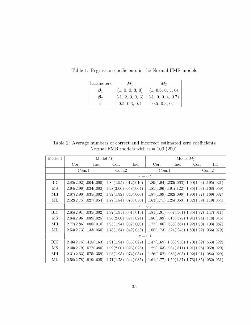
Table 1: Regression coefficients in the Normal FMR models

Parameters M1 M2

β1 (1, 0, 0, 3, 0) (1, 0.6, 0, 3, 0)β2 (-1, 2, 0, 0, 3) (-1, 0, 0, 4, 0.7)π 0.5, 0.3, 0.1 0.5, 0.3, 0.1

Table 2: Average numbers of correct and incorrect estimated zero coefficientsNormal FMR models with n = 100 (200)

Method Model M1 Model M2

Cor. Inc. Cor. Inc. Cor. Inc. Cor. Inc.Com.1 Com.2 Com.1 Com.2

π = 0.5BIC 2.85(2.92) .004(.000) 1.89(1.95) .012(.010) 1.89(1.94) .233(.063) 1.90(1.93) .195(.021)MS 2.94(2.99) .024(.002) 1.98(2.00) .058(.004) 1.85(1.96) .191(.122) 1.85(1.93) .168(.059)MH 2.87(2.90) .035(.002) 1.92(1.92) .046(.000) 1.87(1.89) .262(.096) 1.90(1.87) .169(.037)ML 2.52(2.75) .027(.054) 1.77(1.84) .078(.080) 1.63(1.71) .125(.063) 1.82(1.89) .119(.054)

π = 0.3BIC 2.85(2.91) .035(.002) 1.92(1.95) .001(.013) 1.81(1.91) .607(.361) 1.85(1.92) .147(.011)MS 2.84(2.96) .089(.025) 1.96(2.00) .024(.024) 1.80(1.89) .618(.378) 1.94(1.94) .118(.045)MH 2.77(2.86) .088(.010) 1.95(1.94) .007(.000) 1.77(1.86) .685(.364) 1.92(1.90) .193(.087)ML 2.54(2.73) .133(.050) 1.78(1.84) .042(.053) 1.65(1.73) .524(.245) 1.80(1.92) .056(.079)

π = 0.1BIC 2.46(2.75) .415(.163) 1.91(1.94) .056(.027) 1.47(1.69) 1.08(.956) 1.70(1.82) .553(.322)MS 2.40(2.79) .577(.380) 1.99(2.00) .026(.023) 1.22(1.53) .934(.811) 1.91(1.98) .059(.020)MH 2.31(2.63) .575(.359) 1.93(1.95) .074(.054) 1.26(1.52) .983(.805) 1.92(1.91) .084(.029)ML 2.58(2.78) .919(.625) 1.71(1.78) .044(.085) 1.61(1.77) 1.59(1.37) 1.76(1.85) .052(.051)

35

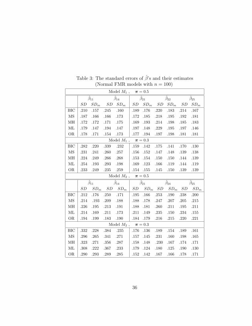
Table 3: The standard errors of β’s and their estimates(Normal FMR models with n = 100)

Model M1 , π = 0.5

β11 β14 β21 β22 β25

SD SDm SD SDm SD SDm SD SDm SD SDm

BIC .210 .157 .245 .160 .189 .176 .220 .183 .214 .167MS .187 .166 .166 .173 .172 .185 .218 .195 .192 .181MH .172 .172 .171 .175 .169 .193 .214 .198 .185 .183ML .179 .147 .194 .147 .197 .148 .229 .195 .197 .146OR .178 .171 .154 .173 .177 .194 .197 .198 .181 .181

Model M1 , π = 0.3BIC .282 .220 .339 .232 .159 .142 .175 .141 .170 .130MS .231 .241 .260 .257 .156 .152 .147 .148 .139 .138MH .224 .249 .266 .268 .153 .154 .150 .150 .144 .139ML .254 .193 .293 .198 .169 .123 .166 .119 .144 .119OR .233 .249 .235 .259 .154 .155 .145 .150 .139 .139

Model M2 , π = 0.5

β11 β14 β21 β24 β25

SD SDm SD SDm SD SDm SD SDm SD SDm

BIC .212 .176 .250 .171 .195 .166 .253 .190 .238 .200MS .214 .193 .209 .188 .188 .178 .247 .207 .205 .215MH .226 .195 .213 .191 .188 .181 .260 .211 .195 .211ML .214 .169 .211 .173 .211 .149 .235 .150 .234 .155OR .194 .199 .183 .190 .184 .179 .216 .215 .220 .221

Model M2 , π = 0.3BIC .332 .228 .384 .235 .176 .136 .189 .154 .189 .161MS .296 .265 .341 .271 .157 .145 .231 .160 .198 .165MH .323 .271 .356 .287 .158 .148 .230 .167 .174 .171ML .308 .222 .367 .233 .179 .124 .180 .125 .190 .130OR .290 .293 .289 .285 .152 .142 .167 .166 .178 .171

36

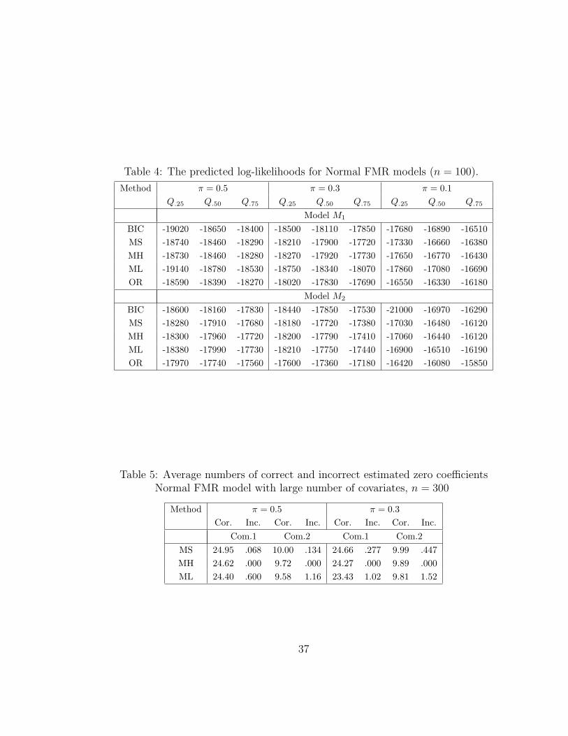
Table 4: The predicted log-likelihoods for Normal FMR models (n = 100).

Method π = 0.5 π = 0.3 π = 0.1Q.25 Q.50 Q.75 Q.25 Q.50 Q.75 Q.25 Q.50 Q.75

Model M1

BIC -19020 -18650 -18400 -18500 -18110 -17850 -17680 -16890 -16510MS -18740 -18460 -18290 -18210 -17900 -17720 -17330 -16660 -16380MH -18730 -18460 -18280 -18270 -17920 -17730 -17650 -16770 -16430ML -19140 -18780 -18530 -18750 -18340 -18070 -17860 -17080 -16690OR -18590 -18390 -18270 -18020 -17830 -17690 -16550 -16330 -16180

Model M2

BIC -18600 -18160 -17830 -18440 -17850 -17530 -21000 -16970 -16290MS -18280 -17910 -17680 -18180 -17720 -17380 -17030 -16480 -16120MH -18300 -17960 -17720 -18200 -17790 -17410 -17060 -16440 -16120ML -18380 -17990 -17730 -18210 -17750 -17440 -16900 -16510 -16190OR -17970 -17740 -17560 -17600 -17360 -17180 -16420 -16080 -15850

Table 5: Average numbers of correct and incorrect estimated zero coefficientsNormal FMR model with large number of covariates, n = 300

Method π = 0.5 π = 0.3Cor. Inc. Cor. Inc. Cor. Inc. Cor. Inc.

Com.1 Com.2 Com.1 Com.2MS 24.95 .068 10.00 .134 24.66 .277 9.99 .447MH 24.62 .000 9.72 .000 24.27 .000 9.89 .000ML 24.40 .600 9.58 1.16 23.43 1.02 9.81 1.52

37

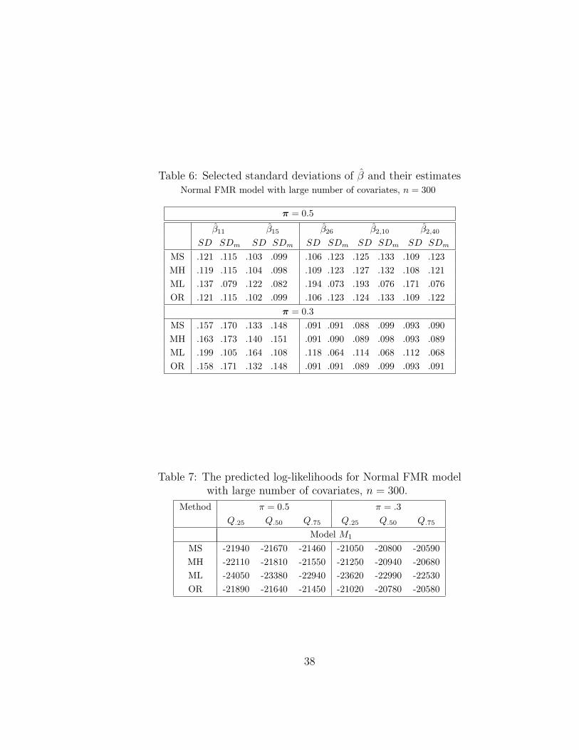
Table 6: Selected standard deviations of β and their estimatesNormal FMR model with large number of covariates, n = 300

π = 0.5

β11 β15 β26 β2,10 β2,40

SD SDm SD SDm SD SDm SD SDm SD SDm

MS .121 .115 .103 .099 .106 .123 .125 .133 .109 .123MH .119 .115 .104 .098 .109 .123 .127 .132 .108 .121ML .137 .079 .122 .082 .194 .073 .193 .076 .171 .076OR .121 .115 .102 .099 .106 .123 .124 .133 .109 .122

π = 0.3MS .157 .170 .133 .148 .091 .091 .088 .099 .093 .090MH .163 .173 .140 .151 .091 .090 .089 .098 .093 .089ML .199 .105 .164 .108 .118 .064 .114 .068 .112 .068OR .158 .171 .132 .148 .091 .091 .089 .099 .093 .091

Table 7: The predicted log-likelihoods for Normal FMR modelwith large number of covariates, n = 300.

Method π = 0.5 π = .3Q.25 Q.50 Q.75 Q.25 Q.50 Q.75

Model M1

MS -21940 -21670 -21460 -21050 -20800 -20590MH -22110 -21810 -21550 -21250 -20940 -20680ML -24050 -23380 -22940 -23620 -22990 -22530OR -21890 -21640 -21450 -21020 -20780 -20580

38

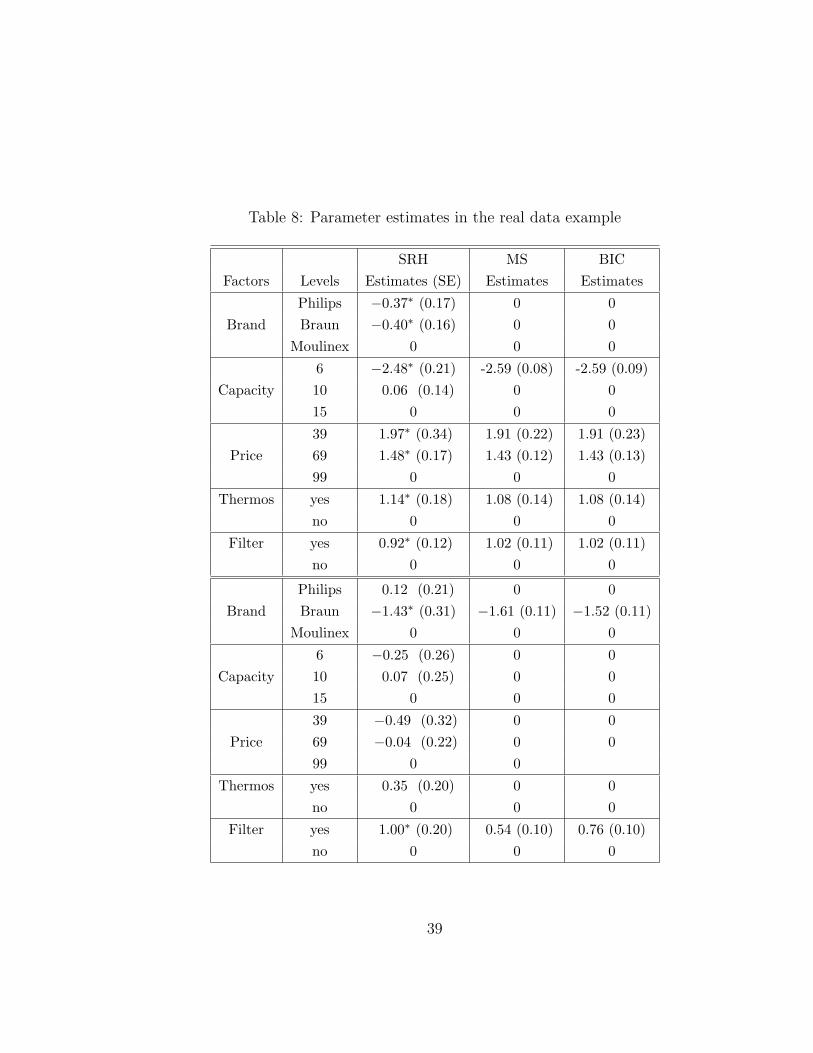
Table 8: Parameter estimates in the real data example

SRH MS BICFactors Levels Estimates (SE) Estimates Estimates

Philips −0.37∗ (0.17) 0 0Brand Braun −0.40∗ (0.16) 0 0

Moulinex 0 0 0

6 −2.48∗ (0.21) -2.59 (0.08) -2.59 (0.09)Capacity 10 0.06 (0.14) 0 0

15 0 0 0

39 1.97∗ (0.34) 1.91 (0.22) 1.91 (0.23)Price 69 1.48∗ (0.17) 1.43 (0.12) 1.43 (0.13)

99 0 0 0

Thermos yes 1.14∗ (0.18) 1.08 (0.14) 1.08 (0.14)no 0 0 0

Filter yes 0.92∗ (0.12) 1.02 (0.11) 1.02 (0.11)no 0 0 0

Philips 0.12 (0.21) 0 0Brand Braun −1.43∗ (0.31) −1.61 (0.11) −1.52 (0.11)

Moulinex 0 0 0

6 −0.25 (0.26) 0 0Capacity 10 0.07 (0.25) 0 0

15 0 0 0

39 −0.49 (0.32) 0 0Price 69 −0.04 (0.22) 0 0

99 0 0

Thermos yes 0.35 (0.20) 0 0no 0 0 0

Filter yes 1.00∗ (0.20) 0.54 (0.10) 0.76 (0.10)no 0 0 0

39