Variable exponent functionals in image restoration

Applied Mathematics and Computation 216 (2010) 870–882

Contents lists available at ScienceDirect

Applied Mathematics and Computation

journal homepage: www.elsevier .com/ locate /amc

Variable exponent functionals in image restoration

Fang Li a,*, Zhibin Li b, Ling Pi c

a Department of Mathematics, East China Normal University, Dongchuan Rd. Minhang, Shanghai 200241, Chinab Department of Computer Science, East China Normal University, Shanghai 200241, Chinac Department of Mathematics, Shanghai Jiao Tong University, Shanghai 200240, China

a r t i c l e i n f o

Keywords:Variable exponent functionalBV spaceStaircasing effectHeat flow

0096-3003/$ - see front matter � 2010 Elsevier Incdoi:10.1016/j.amc.2010.01.094

* Corresponding author.E-mail address: [email protected] (F. Li).

a b s t r a c t

We study a functional with variable exponent, 1 < pðxÞ 6 2, which provides a model forimage denoising and restoration. Here pðxÞ is defined by the gradient information in theobserved image. The diffusion derived from the proposed model is between total variationbased regularization and Gaussian smoothing. The diffusion speed of the correspondingheat equation is tuned by the variable exponent pðxÞ. The minimization problem and itsassociated flow in a weakened formulation are discussed. The existence, uniqueness, stabil-ity and long-time behavior of the proposed model are established in the variable exponentfunctional space W1;pðxÞ. Experimental results illustrate the effectiveness of the model inimage restoration.

� 2010 Elsevier Inc. All rights reserved.

1. Introduction

Image denoising is one of the fundamental problems in image processing with numerous applications. The aim of imagedenoising is to design methods which can selectively smooth a noisy image without losing significant features such as edges.

Variational denoising methods are widely studied numerically and theoretically in recent years. In variational framework,the denoising problem can be expressed as follows: given an original image f, it is assumed that it has been corrupted bysome additive noise n. Then the problem is to recover the true image u from

f ¼ uþ n:

Let us consider the following representative minimization problem

min EðuÞ ¼Z

Xjrujpdxþ k

2

ZXðu� f Þ2dx

� �; ð1:1Þ

where 1 6 p 6 2 is a constant and k is a scalar parameter. The first term in the energy functional of (1.1) is a regularizationterm and the second term is a fidelity term. As p ¼ 1, it is the widely used Rudin–Osher–Fatemi (ROF) model proposed in1992 [12]. The considerable advantage of the ROF model is that it can well preserve edge sharpness and location whilesmooth out noise. Mathematically, it is reasonable since its solution belongs to bounded variation (BV) space which allowsdiscontinuities in functions. However, the ROF model favors solutions that are piecewise constant which often causes thestaircasing effect [11,14,15]. The staircasing effect creates false edges which are misleading and not satisfactory in visualeffects.

Choosing p ¼ 2 in (1.1) results in isotropic diffusion which solves the staircasing effect problem but it oversmoothesimages such that the edges are blurred and dislocated. A fixed value of 1 < p < 2 results in anisotropic diffusion between

. All rights reserved.

http://dx.doi.org/10.1016/j.amc.2010.01.094

mailto:[email protected]

http://www.sciencedirect.com/science/journal/00963003

http://www.elsevier.com/locate/amc

F. Li et al. / Applied Mathematics and Computation 216 (2010) 870–882 871

the ROF model and the isotropic smoothing. However, there is a trade-off between piecewise smooth regions reconstructionand edge preservation.

Since different values of p should have different advantages, it encourages one to combine their benefits with a variableexponent. Blomgren et al. proposed the following minimization problem in [1]

minfEðuÞ ¼Z

XjrujpðjrujÞdxg; ð1:2Þ

where lims!0pðsÞ ¼ 2; lims!1pðsÞ ¼ 1, and p is a monotonically decreasing function. This model is a variable exponent model.It chooses diffusion speed through exponent and then can reduce the staircasing effect. Since p depends on ru, it is hard toestablish the lower semi-continuity of the energy functional. Bollt et al. proved that this problem with an L1 or L2 norm fidel-ity term has a minimizer in [2], however, nothing about the associated heat equations was discussed.

Later, Chen et al. proposed the following model in [3]

minu2BVðXÞ\L2ðXÞ EðuÞ ¼Z

Xuðx;DuÞ þ k

2

ZXðu� f Þ2dx

� �; ð1:3Þ

where

uðx; rÞ ¼1

qðxÞ jrjqðxÞ; jrj 6 b;

jrj � bqðxÞ�bqðxÞ

qðxÞ ; jrj > b;

8<:

qðxÞ ¼ 1þ 11þkjrGr�f ðxÞj ; GrðxÞ ¼ 1ffiffiffiffi

2pp

r exp jxj22r2

� �is the Gaussian kernel, k > 0; r > 0 are fixed parameter, and b is a user-defined

threshold. Mathematically, the energy minimization problem and the associated heat flow were discussed.Inspired by the above models, we propose the model

minu2W1;pðxÞðXÞ\L2ðXÞ EpðxÞðuÞ ¼Z

X

1pðxÞ jrujpðxÞdxþ k

2

ZXðu� f Þ2dx

� �; ð1:4Þ

where pðxÞ ¼ 1þ gðxÞ and gðxÞ ¼ 11þkjrGr�f ðxÞj.

Clearly in the regions with edges, g ! 0 since the image gradient is large, model (1.4) approximates the ROF model, so theedges will be preserved; In relatively smooth regions g ! 1 since image gradient is small, model (1.4) approximates isotropicsmoothing, so they will be processed into piecewise smooth regions. In other regions, the diffusion is properly adjusted bythe function pðxÞ.

The proposed model (1.4) is simpler than (1.3) in the formulation. Meanwhile, model (1.4) is more automatic than (1.3)since no user-defined threshold b is needed in (1.4). Chen et al. studied problem (1.3) in BV framework [3], however, in thispaper we will study problem (1.4) in the variable exponent space W1;pðxÞ.

The paper is organized as follows: in Section 2 we give some important lemmas and then prove the existence and unique-ness of the solution of the minimization problem (1.4). In Section 3 we prove the existence, uniqueness and stability of thesolution of the heat flow problem and discuss the long-time behavior. In Section 4 we provide our numerical algorithm andexperimental results to illustrate the effectiveness of our model in image restoration. Finally, we conclude the paper in Sec-tion 5.

2. The minimization problem

Let X � Rn be a bounded open set with Lipschitz boundary, f 2 L1ðXÞ. By the definition of gðxÞ and Gaussian convolution,we obtain rGr � f 2 C1ðXÞ. Then there exists a constant M > 0, such that jrGr � f j 6 M. Therefore, gðxÞP 1

1þM2 andpðxÞP 1þ 1

1þM2 > 1. Meanwhile, since gðxÞ 6 1, we get 1 < pðxÞ 6 2 in the proposed model (1.4).Variable exponent spaces. Let pðxÞ : X! ½1;þ1Þ be a measurable function, called variable exponent on X. By PðXÞ we de-

note the family of all measurable functions on X. Let p� :¼ ess infX

pðxÞ; pþ :¼ ess supX

pðxÞ. We define a functionalZ
Q pðxÞðuÞ ¼
XjujpðxÞdx

and a norm by formula

kukpðxÞ ¼ kukLpðxÞðXÞ :¼ inffk > 0 : Q pðxÞðu=kÞ 6 1g:

Then the variable exponent Lebesgue space LpðxÞðXÞ and the variable exponent Sobolev space W1;pðxÞðXÞ are defined as

LpðxÞðXÞ ¼ fu : X! RjkukpðxÞ <1g;

W1;pðxÞðXÞ ¼ fu : X! Rju 2 LpðxÞðXÞ;ru 2 LpðxÞðXÞg:

With the norm kuk1;pðxÞ ¼ kukpðxÞ þ krukpðxÞ;W1;pðxÞðXÞ becomes a Banach space. W1;pðxÞ

0 ðXÞ denotes the closure of C10 ðXÞ underthe norm k � k1;pðxÞ. See [4] for the basic theory of variable exponent spaces.

872 F. Li et al. / Applied Mathematics and Computation 216 (2010) 870–882

In the following, we cite Lemmas 2.1 and 2.2 from [8]. Then we prove Lemmas 2.3–2.5 as the preparation for the proof ofthe main theorems.

Lemma 2.1. Let pðxÞ; qðxÞ 2 PðXÞ, and for a.e. x 2 X we have pðxÞ 6 qðxÞ. Then LqðxÞðXÞ,!LpðxÞðXÞ;W1;qðxÞðXÞ,!W1;pðxÞðXÞ. Thenorm of the embedding operator does not exceed 1þ jXj, where jXj denotes the measure of X.

Lemma 2.2. Let pðxÞ 2 PðXÞ, 1 < p� 6 pþ <1. Then LpðxÞðXÞ;W1;pðxÞðXÞ and W1;pðxÞ0 ðXÞ are all reflexive Banach spaces.

Lemma 2.3. Let Fðru;u; xÞ ¼ 1pðxÞ jrujpðxÞ þ k

2 ðu� f Þ2; pðxÞ ¼ 1þ gðxÞ as in model (1.4). Then for each z; x, Fðn; z; xÞ is convex in n.

Proof. As we know, if a multivariable function GðxÞ; x ¼ ðx1; . . . ; xnÞ is twice differentiable, then G is convex if and only if theHessian matrix r2GðxÞ ¼ @2G

@xi@xjðxÞ is semi-positively definite for abitrary x 2 domðGÞ. Let Fðn; z; xÞ ¼ 1

pðxÞ jnjpðxÞ þ k

2 ðz� f Þ2. Then

Fni¼ 1

pðxÞ pðxÞjnjpðxÞ�1 ni

jnj ¼ jnjpðxÞ�2ni;

Fninj¼ ðpðxÞ � 2ÞjnjpðxÞ�4ninj þ jnjpðxÞ�2dij;

Fninjgigj ¼ ðpðxÞ � 2ÞjnjpðxÞ�4ninjgigj þ jnjpðxÞ�2dijgigj; 8g 2 Rn;

where the same upper and lower index denotes summation from 1 to n. By Cauchy inequality

ninjgigj ¼X

nigi

� �26

Xn2

i

� � Xg2

i

� �¼ jnj2jgj2

and the condition 1 < pðxÞ 6 2, we obtain

Fninjgigj P ðpðxÞ � 2ÞjnjpðxÞ�4jnj2jgj2 þ jnjpðxÞ�2jgj2 ¼ ðpðxÞ � 1ÞjnjpðxÞ�2jgj2 P 0:

Therefore, F is convex in n. h

Lemma 2.4. Let Fðn; z; xÞ be bounded from below, and the map n#Fðn; z; xÞ is convex in each z 2 R; x 2 X. Then the energy func-tional IðuÞ :¼

RX Fðru;u; xÞdx is weakly lower semi-continuous in W1;pðxÞðXÞ.

Mimicking the proof of Theorem 1 (p. 446 in [4]) in which p is a constant, we can prove the variable exponent case whichis Lemma 2.4. In the proof, we need the Sobolev embedding W1;pðxÞðXÞ,!LpðxÞðXÞ. Fortunately, under the assumption of thispaper, the Sobolev embedding holds. It is the following lemma.

Lemma 2.5. Let the dimension of X be n ¼ 2;1 6 p� 6 pðxÞ 6 pþ 6 2. Then the embedding W1;pðxÞ,!LpðxÞ is compact.

Proof. From n ¼ 2, we deduce that ðp�Þ� ¼ np�

n�p� ¼ nn=p��1 P n

n�1 ¼ 2 P pþ. Since X is bounded open set with Lipschitz bound-

ary, by the Sobolev embedding theorem (where p is constant) in [4] and Lemma 2.1, we obtain

W1;pðxÞðXÞ,!W1;p� ðXÞ,!LpþðXÞ,!LpðxÞðXÞ;

where the embedding W1;p� ðXÞ,!LpþðXÞ is compact. Therefore, the embedding W1;pðxÞðXÞ,!LpðxÞðXÞ is compact.Note that in our model (1.4), pðxÞ ¼ 1þ gðxÞ. By definition of gðxÞ, we have 1 < p� 6 pðxÞ 6 pþ 6 2, which satisfies the

condition of Lemma 2.5. Similar results are also established in [5,6]. h

Theorem 2.1. Let X � R2 be a bounded open set with Lipschitz boundary, f 2W1;pðxÞðXÞ \ L2ðXÞ. Then the minimization problem

minu2W1;pðxÞðXÞ\L2ðXÞ

EpðxÞðuÞ ¼Z

X


2

ZXðu� f Þ2dx

� �

has a unique minimizer u 2W1;pðxÞðXÞ \ L2ðXÞ.

Proof. Let l ¼ infv2W1;pðxÞðXÞ\L2ðXÞ

EpðxÞðvÞ. Since f 2W1;pðxÞðXÞ \ L2ðXÞ;l is finite. Let fukg1k¼1;uk 2W1;pðxÞðXÞ \ L2ðXÞ be the mini-

mizing sequence such that EpðxÞðukÞ ! l. Then there exists a constant C, such that
ZX
1pðxÞ jrukjpðxÞdx 6 C and

ZXðuk � f Þ2dx 6 C:

HenceR

XðukÞ2dx 6 C. By Lemma 2.1, L2ðXÞ � LpðxÞðXÞ. So we haveR

X jujpðxÞdx 6 C.

Together with the inequality
ZXjrukjpðxÞdx 6 C
ZX

1pþjrukjpðxÞdx 6 C

ZX

1pðxÞ jrukjpðxÞdx 6 C;


we obtain QpðxÞðukÞ þ Q pðxÞðrukÞ 6 C. This implies that fukg1k¼1 is a uniformly bounded sequence in W1;pðxÞðXÞ. Meanwhile,fukg1k¼1 is uniformly bounded in L2ðXÞ. Since W1;pðxÞðXÞ \ L2ðXÞ is a reflexive Banach space, there exists a subsequencefukjg1j¼1 � fukg1k¼1, and a function u 2W1;pðxÞðXÞ \ L2ðXÞ, such that

ukj* u in W1;pðxÞðXÞ \ L2ðXÞ:

By Lemma 2.4, EpðxÞ is weakly lower semi-continuous in W1;pðxÞðXÞ \ L2ðXÞ. Then we have

EpðxÞðuÞ 6 lim infj!1

EpðxÞðukjÞ ¼ l:

Therefore, u is a minimizer of EpðxÞ. The uniqueness follows from the strict convexity of EpðxÞðuÞ about u. h

Theorem 2.2. Let X � R2 be a bounded open set with Lipschitz boundary, w 2W1;pðxÞðXÞ \ L1ðXÞ; f �w 2W1;pðxÞ0 ðXÞ \ L1ðXÞ.

Then the minimization problem

minu2W1;pðxÞðXÞ\L2ðXÞ; u�w2W1;pðxÞ

0

EpðxÞðuÞ ¼Z

X


2

ZXðu� f Þ2dx

� �ð2:1Þ

has a unique minimizer u 2W1;pðxÞðXÞ \ L1ðXÞ, which satisfies u�w 2W1;pðxÞ0 ðXÞ \ L1ðXÞ.

Proof. Let u 2 Uð¼W1;pðxÞðXÞ \ L2ðXÞÞ and denote a ¼maxfkwk1; kfk1g. Let ua be the function u which has been cut-off at�a and a, i.e. ua ¼minfa;maxf�a;ugg. By definition of a, it is easy to see that ua �w 2W1;pðxÞ

0 ðXÞ \ L2ðXÞ. Moreover,

rua ¼ru; juj 6 a;

0; juj > a:

�

Hence jruaj 6 jruj a:e: x 2 X and so EpðxÞðuaÞ 6 EpðxÞðuÞ. It follows that it suffices to look for minimizers in the setUa ¼ fua : u 2 Ug.Let l ¼ inf

v2Ua

EpðxÞðvÞ, and fukg1k¼1 � Ua be a minimizing sequence. Then EpðxÞðukÞ ! l. Hence
ZX
1pðxÞ jrukjpðxÞdx 6 C;

ZXðuk � f Þ2dx 6 C:

By the W1;1 – Sobolev–Poincaré inequality, the embedding LpðxÞðXÞ,!L1ðXÞ and the fact uk �w 2W1;10 ðXÞ, we get
Z
XjukjpðxÞdx ¼

ZXjukjpðxÞ�1jukjdx 6 apþ�1

ZXjukjdx 6 C

ZXjuk �wj þ jwjdx 6 C

ZXjruk �rwjdxþ C 6 C

ZXjrukjdxþ C

6 CZ

XjrukjpðxÞdxþ C 6 C

ZX

1pþjrukjpðxÞdxþ C 6 C

ZX

1pðxÞ jrukjpðxÞdxþ C 6 C:

Together with the inequality
ZXjrukjpðxÞdx 6 C;
we obtain Q pðxÞðukÞ þ QpðxÞðrukÞ 6 C, which implies fukg1k¼1 is uniformly bounded in W1;pðxÞðXÞ. Meanwhile,R

Xðuk � f Þ2dx 6 Cresults in the uniformly boundedness of fukg1k¼1 in L2ðXÞ. Since W1;pðxÞðXÞ \ L2ðXÞ is a reflexive Banach space, there exists asubsequence fukj

g1j¼1 � fukg1k¼1, and u 2W1;pðxÞðXÞ \ L2ðXÞ such that

ukj* u in W1;pðxÞðXÞ \ L2ðXÞ:

Moreover, since fukg1k¼1 � Ua, we conclude that u 2W1;pðxÞ \ L1ðXÞ. We assert next that, u�w 2W1;pðxÞ0 \ L1ðXÞ. To see

this, note that for w 2W1;pðxÞðXÞ \ L1ðXÞ;uk �w 2W1;pðxÞ0 ðXÞ \ L1ðXÞ. Since W1;pðxÞ

0 ðXÞ \ L1ðXÞ is a closed, linear subspaceof W1;pðxÞðXÞ \ L1ðXÞ, it is weakly closed. Hence u�w 2W1;pðxÞ

0 ðXÞ \ L1ðXÞ. Then by Lemma 2.4,

EpðxÞðuÞ 6 lim infj!1

EpðxÞðukjÞ ¼ l:

Therefore, we conclude that u is a minimizer of EpðxÞ. The uniqueness follows from the strictly convexity of EpðxÞðuÞ in u.In the proof of Theorem 2.2, we use W1;1 – Sobolev–Poincaré inequality which is different from Theorem 2.1. In special

case with no fidelity term in the energy (called pðxÞ-Laplacian Dirichlet problem), the existence of minimizer has beenstudied in [5,7].

Assume w 2W1;pðxÞðXÞ \ L1ðXÞ, and f �w 2W1;pðxÞ0 ðXÞ \ L1ðXÞwhich means f has fixed boundary value f j@X ¼ wj@X. Let u

be the minimizer of problem (2.1). We calculate the corresponding Euler–Lagrange equation.Taking u 2W1;pðxÞ

0 ðXÞ as a test function, we have uþ �u�w 2W1;pðxÞ0 ðXÞ for each � > 0. Then


dd�

��¼0

EpðxÞðuþ �uÞ ¼d

d�

��¼0

ZX

1pðxÞ jruþ �rujpðxÞdxþ k

2

ZXðuþ �u� f Þ2dx

� �

¼Z

Xjruþ �rujpðxÞ�1 ruþ �ru

jruþ �rujruþ kðuþ �u� f Þudx� ��

�¼0

¼Z

XjrujpðxÞ�2ruruþ kðu� f Þudx ¼ 0:

We have that the minimizer of problem (2.1) satisfies the following equation with Dirichlet boundary condition:

divðjrujpðxÞ�2ruÞ � kðu� f Þ ¼ 0; x 2 X;

u ¼ w: x 2 @X:

(

Similarly, the minimizer of problem (1.4) satisfies the following equation with Neumann boundary condition

divðjrujpðxÞ�2ruÞ � kðu� f Þ ¼ 0; x 2 X;@u@N ¼ 0; x 2 @X;

(

where N denotes the unit outward normal of @X.In [13], entropy solution for the pðxÞ-Laplace equation without fidelity term was studied. In a different perspective, we

study the associated flow corresponding to the Euler–Lagrange equation in this paper. In the following, we only study theproblem with Neumann boundary condition. Remark that Neumann or periodic boundary conditions are more natural forimage processing applications. However, the Dirichlet boundary conditions are a bit more interesting mathematically and allof the same proofs hold (in a simplified manner) for the Neumann conditions. h

3. The associated heat flow to problem (1.4)

Using the steepest descent method, the associated heat flow to problem (1.4) is given by

ut ¼ divðjrujpðxÞ�2ruÞ � kðu� f Þ; ðx; tÞ 2 XT ; ð3:1Þ@u@N¼ 0; ðx; tÞ 2 @XT ; ð3:2Þ

uð0Þ ¼ f ; ðx; tÞ 2 X� ft ¼ 0g: ð3:3Þ

Firstly, we derive another definition of weak solution of problem (3.1)–(3.3). Denote

Fðru;u; xÞ ¼ 1pðxÞ jrujpðxÞ þ k

2ðu� f Þ2:

Then (3.1) is equivalent to ut ¼ �F 0ðru;u; xÞ, where F 0ðru;u; xÞ denotes the Gateaux derivative of F about u.Suppose u be a classical solution of (3.1)–(3.3). For each v 2 L2ð0; T; W1;pðxÞðXÞ \ L2ðXÞÞ, multiplying (3.1) by v � u, and

then integrating over X, we have that
ZX
utðv � uÞdx ¼Z

X�F 0ðru; u; xÞðv � uÞdx:

From the convexity of Fðru; u; xÞ, we deduce that
ZX
utðv � uÞdxþ EpðxÞðvÞP EpðxÞðuÞ: ð3:4Þ

Integrating over [0,s] for any s 2 ½0; T� yields
Z s
0

ZX

utðv � uÞdxdt þZ s

0EpðxÞðvÞdt P

Z s

0EpðxÞðuÞdt: ð3:5Þ

On the other hand, if (3.5) holds, setting v ¼ uþ �u in (3.5) with u 2 C10 ðXÞ, we obtain
Z s
0

ZX

ut�udxdt þZ s

0EpðxÞðuþ �uÞdt P

Z s

0EpðxÞðuÞdt;

which impliesR s

0

RX ut�udxdt þ

R s0 EpðxÞðuþ �uÞdt attains its minimum at � ¼ 0. Hence

dd�

��¼0

Z s

0

ZX

ut�udxdt þZ s

0EpðxÞðuþ �uÞdt

� ¼ 0;


that is,
Z s
0

ZX

_uudxdt þZ s

0

ZX

F 0ðru; u; xÞudxdt ¼ 0:

Since u is arbitrary, _uþ F 0ðru;u; xÞ ¼ 0. That is to say, if u satisfies (3.5), then u is a weak solution of (3.1) in the sense ofdistribution. This motivates us to give the following definition.

Definition. A function u 2 L2ð0; T; W1;pðxÞðXÞ \ L2ðXÞÞ, with _u 2 L2ðXTÞ is called a weak solution of Eqs. (3.1)–(3.3) if uð0Þ ¼ f ,and for all v 2 L2ð0; T; W1;pðxÞðXÞ \ L2ðXÞÞ, for all s 2 ½0; T�, (3.5) holds.

Let uðnÞ ¼ 1pðxÞ jnj

pðxÞ, then the derivative is urðnÞ ¼ jnjpðxÞ�2n. Setting

u�ðnÞ ¼ 1pðxÞ

ffiffiffiffiffiffiffiffiffiffiffiffiffiffiffiffiffiffijnj2 þ �2

q� pðxÞ

with 0 < � < 1. Then

u�r ðnÞ ¼

nffiffiffiffiffiffiffiffiffiffiffiffiffiffiffiffiffiffijnj2 þ �2

q� 2�pðxÞ :

It is easy to see that u�ðnÞ is convex in n and u� ! u as �! 0.To prove the existence of solution to (3.1)–(3.3), we first discuss the solution of the approximated problem

ut ¼ �Duþ divðu�r ðruÞÞ � kðu� fdÞ; ðx; tÞ 2 XT ; ð3:6Þ

@u@N¼ 0; ðx; tÞ 2 @XT ; ð3:7Þ

uð0Þ ¼ fd; ðx; tÞ 2 X� ft ¼ 0g; ð3:8Þ

where fd 2 C1ðXÞ has the following properties:

fd ! f in L2ðXÞ; kfdkL1ðXÞ 6 kfkL1ðXÞ; uðrfdÞ 6 uðrf Þ: ð3:9Þ

Since 1 < pðxÞ 6 2, for uðsÞ ¼ 1pðxÞ s

pðxÞ, we have u0ðsÞ ¼ 1pðxÞpðxÞspðxÞ�1 ¼ spðxÞ�1 > 0ðs > 0Þ. Hence u is monotonically increasing

function in s ðs > 0Þ. The convexity of u yields

u�ðrfdÞ ¼1

pðxÞ

ffiffiffiffiffiffiffiffiffiffiffiffiffiffiffiffiffiffiffiffiffiffiffijrfdj2 þ �2

q� pðxÞ

61

pðxÞ ðjrfdj þ �ÞpðxÞ 61

pðxÞ2pðxÞ�1ðjrfdjpðxÞ þ �pðxÞÞ

6 2pðxÞ�1 uðrfdÞ þ1

pðxÞ �pðxÞ

� 6 2ðuðrf Þ þ �Þ: ð3:10Þ

The existence of fd can be proved by the standard argument as in [10].

Lemma 3.1. The problem (3.6)–(3.8) has a unique weak solution u�d, with u�d 2 L1ð0; T; W1;pðxÞðXÞ \ L2ðXÞÞ and _u�d 2L2ð0; T; L2ðXÞÞ such that
Z 1
0

ZXj _u�dj

2dxdt þ supt>0

ZX

�2jru�dj

2 þu�ðru�dÞ þk2ðu�d � fdÞ2dx

� �6 2

ZX

�2jrfdj2dxþuðrf Þdxþ 1

� �: ð3:11Þ

Proof. (3.6)–(3.8) is quasilinear parabolic equations of divergence type. Since it satisfies all necessary conditions which canbe verified by directly calculation, (3.6)–(3.8) has a unique weak solution u�d [9]. Then u�d satisfies (3.6). Multiplying (3.6) by _u�dand integrating on X, we get

ZXj _u�dj

2 ¼Z

X� _u�dDu�ddxþ

ZX

_u�ddivðu�r ðru�dÞÞdx� k

ZX

_u�dðu�d � fdÞdx:

Then
ZXj _u�dj
2dxþ ddt

ZX

�2jru�dj


� �¼ 0:

Integrating the above formula on (0, t),
Z s
0

ZXj _u�dj

2dxdt þZ

X

�2jru�dj


� �¼

ZX

�2jrfdj2 þu�ðrfdÞ þ

k2ðfd � fdÞ2dx

� �:


Therefore,
Z 1
0

ZXj _u�dj

2dxdt þ supt>0

ZX

�2jru�dj


� �6 2

ZX

�2jrfdj2 þu�ðrfdÞdx

� �:

Since 0 < � < 1, we get the conclusion. h

Lemma 3.2. Let f 2W1;pðxÞ \ L1ðXÞ, and u�d be the weak solution of the problem (3.6)–(3.8). Then

ku�dkL1ðXT Þ 6 kfkL1ðXÞ: ð3:12Þ

Proof. Let G be a truncation function of class C1 such that GðtÞ ¼ 0 on ð�1;0�, and G is strictly increasing in ½0;þ1Þ, andG0 6 M where M is a constant. Let k ¼ kfkL1ðXÞ and set v ¼ Gðu�d � kÞ. Since u�d 2W1;pðxÞðXÞ \ L2ðXÞ, by the chain rule we getv 2W1;pðxÞðXÞ \ L2ðXÞ, and rv ¼ G0ðu�d � kÞru�d. Multiplying (3.6) by v and integrating over X yields

0 ¼Z

X

_u�dGðu�d � kÞdxþ �Z

Xjru�dj

2G0ðu�d � kÞdxþZ

Xu�

r ðru�dÞru�dG0ðu�d � kÞdxþ kZ

Xðu�d � fdÞGðu�d � kÞdx: ð3:13Þ

By the definition of u�;R

X u�r ðru�dÞru�dG0ðu�d � kÞdx P 0. It is obvious that �

RX jru�dj

2G0ðu�d � kÞdx P 0. IfR

Xðu�d � fdÞGðu�d � kÞdx 6 0, then we get u�d 6 kfdkL1ðXÞ 6 kfkL1ðXÞ ¼ k. Otherwise, we have

RXðu�d � fdÞGðu�d � kÞdx P 0. Hence (3.13) yields
Z
X

_u�dGðu�d � kÞdx 6 0:

Since 0 6 G0 6 M we deduce that

ddt

ZXðGðu�d � kÞÞ2dx 6 0:

ThereforeR

XðGðu�d � kÞÞ2dx is monotonically decreasing function about t and then
ZXðGðu�d � kÞÞ2dx 6
ZXðGðu�d � kÞÞ2dxjt¼0 ¼

ZXðGðfd � kÞÞ2dx ¼ 0:

So we have proved that u�d 6 k. Similarly, u�d P �k can be proved. h

Theorem 3.1 (existence and uniqueness). Suppose f 2W1;pðxÞðXÞ \ L1ðXÞ. Then (3.1)–(3.3) has a unique weak solutionu 2 L1ð0; T;W1;pðxÞðXÞ \ L1ðXÞÞ, with _u 2 L2ðXTÞ.

Proof. First we fix d > 0 and pass to the limit �! 0. Let fu�dg be the sequence of solution to (3.6)–(3.8). By (3.11) and (3.12),we get that fu�dg has uniformly bounded L1ðX1Þ norm about �, and f _u�dg has uniformly bounded L2ðX1Þ norm. Then thereexists a subsequence, also denoted by fu�dg, and a function ud 2 L1ðX1Þ, such that as �! 0,

u�d * ud weakly � in L1ðX1Þ; ð3:14Þ_u�d * w weakly in L2ðX1Þ: ð3:15Þ

The same argument used in the proof of Lemma 3.1 [16] gives us that _ud ¼ w;udð0Þ ¼ fd. Then we have _ud 2 L2ðX1Þ.Moreover, for all / 2 L2ðXÞ,
Z
Xðu�dð�; tÞ� fdÞ/ðxÞdx¼

Z t

0

ZX

_u�dðx;sÞ1½0;t�ðsÞ/ðxÞdxds!Z t

0

ZX

_udðx;sÞ1½0;t�ðsÞ/ðxÞdxdt¼Z

Xðudð�; tÞ� fdÞ/ðxÞdx ð�! 0Þ;

which implies that

u�dð�; tÞ* udð�; tÞ weakly in L2ðXÞ:

From (3.11), for each t > 0; fu�dð�; tÞg is a uniformly bounded sequence in W1;1ðXÞ. Then there exists a subsequence, alsodenoted by fu�dð�; tÞg, such that

u�dð�; tÞ ! udð�; tÞ strongly in L1ðXÞ: ð3:16Þ

From (3.12), (3.14) and (3.16), we obtain
ZXju�dð�; tÞ � udð�; tÞj2dx 6 ku�dð�; tÞ � udð�; tÞkL1ðXÞ
ZXju�dð�; tÞ � udð�; tÞjdx 6 CkfkL1ðXÞ

ZXju�dð�; tÞ

� udð�; tÞjdxdt ! 0 ðas �! 0Þ:


Therefore,

u�dð�; tÞ ! udð�; tÞ strongly in L2ðXÞ: ð3:17Þ

For all v 2 L2ðð0;1Þ; H1ðXÞÞ, multiplying (3.6) (where u is replaced by u�d) by ðv � u�dÞ and using the convexity of u�, we get
Z s
0

ZX

_u�dðv � u�dÞ þ�2jrv j2 þu�ðrvÞ þ k

2ðv � fdÞ2dxdt P

Z s

0

ZX

�2jru�dj

2 þu�ðru�dÞ þk2ðu�d � fdÞ2dxdt:

From (3.15), (3.17) and the lower semi-continuity of u� we obtain
Z s
0

ZX

_u�dðv � u�dÞ þu�ðrvÞ þ k2ðv � fdÞ2dxdt P lim inf

�!0

Z s

0

ZXu�ðru�dÞ þ

k2ðu�d � fdÞ2dxdt:

Letting �! 0, we obtain that
Z s
0

ZX

_udðv � udÞ þuðrvÞ þ k2ðv � fdÞ2dxdt P

Z s

0

ZXuðrudÞ þ

k2ðud � fdÞ2dxdt ð3:18Þ

holds for all v 2 L2ð0;1; H1ðXÞÞ. By approximation, (3.18) still holds for any v 2 L2ðð0;1Þ; W1;pðxÞðXÞ \ L2ðXÞÞ.It remains to pass to the limit as d! 0. In (3.11) we let �! 0 to get that
Z 1
0

ZXj _udj2dxdt þ sup

t>0

ZX

uðrudÞ þk2ðud � fdÞ2dx

� �6 C;

where C depends on f. Therefore, fudg is uniformly bounded in L1ð0;1; W1;pðxÞðXÞ \ L2ðXÞÞ, and then uniformly bounded inW1;1ðXÞ. We also have _ud is uniformly bounded in L2ðX1Þ. Moreover, letting �! 0 in (3.12) yields

kudkL1ðX1Þ 6 kfkL1ðXÞ:

Hence fudg is uniformly bounded in L1ðX1Þ. By the same argument used in (3.14), (3.15) and (3.17), there exists a subse-quence, also denoted by fudg and a function u 2 L1ðð0;1Þ; W1;pðxÞðXÞ \ L1ðXÞÞ; _u 2 L2ðX1Þ such that as d! 0,

ud * u weakly � in L1ðX1Þ; ð3:19Þ_ud * _u weakly in L2ðX1Þ; ð3:20Þudð�; tÞ ! uð�; tÞ strongly in L2ðXÞ and uniformly for t: ð3:21Þ

Using the lower semi-continuity of u and (3.19)–(3.21), and letting d! 0 in (3.18), we conclude that for allv 2W1;pðxÞðXÞ \ L2ðXÞ
Z s
0

ZX

utðv � uÞdxdt þZ s

0EpðxÞðvÞdt P

Z s

0EpðxÞðvÞdt:

By definition, u is the weak solution of problem (3.1)–(3.3).Uniqueness follows directly from the following stability theorem by letting f1 ¼ f2. h

Theorem 3.2 (stability). Assume u1 and u2 are both weak solutions of (3.1)–(3.3) with initial values f1; f2 2W1;pðxÞðXÞ \ L1ðXÞ.Then for any t > 0,

ku1 � u2kL1ðXÞ 6 kf1 � f2kL1ðXÞ:

Proof. Set k ¼ kf1 � f2kL1ðXÞ. Define

v ¼ u1 � ðu1 � u2 � kÞþw ¼ u2 þ ðu1 � u2 � kÞþ

(;

where

ðu1 � u2 � kÞþ ¼u1 � u2 � k; if u1 � u2 � k P 0;0; otherwise:

�

Then

rv ¼ru1; u1 � u2 6 k;ru2; u1 � u2 P k;

�rw ¼

ru2; u1 � u2 6 k;ru1: u1 � u2 P k:

�

By the definition of weak solution of (3.1)–(3.3), for all t > 0, we have


ZX

_u1ðv � u1Þ þuðrvÞ þ k2ðv � f1Þ2dxdt P

ZXuðru1Þ þ

k2ðu1 � f1Þ2dxdt;Z

X

_u2ðw� u2Þ þuðrwÞ þ k2ðw� f2Þ2dxdt P

ZXuðru2Þ þ

k2ðu2 � f2Þ2dxdt:

Taking summation yields
ZX
_u1ðv � u1Þ þ _u2ðw� u2Þ þuðrvÞ þuðrwÞ þ k2ðv � f1Þ2 þ

k2ðw� f2Þ2dxdt

PZ

Xuðru1Þ þuðru2Þ þ

k2ðu1 � f1Þ2 þ

k2ðu2 � f2Þ2dxdt:

By the definition of v and w, it is clear that

uðrvÞ þuðrwÞ ¼ uðru1Þ þuðru2Þ;

and
ZXðu1 � f1Þ2 þ ðu2 � f2Þ2 � ðv � f1Þ2 � ðw� f2Þ2dx ¼
ZXðu1 � f1Þðu1 þ v � 2f 1Þ þ ðu2 �wÞðu2 þw� 2f 2Þdx

¼Z

Xðu1 � u2 � kÞþ 2u1 � 2f 1 � 2u2 þ 2f 2 � 2ðu1 � u2 � kÞþ

�dx

¼Z

X2ðu1 � u2 � kÞþððu1 � u2 � kÞ � ðu1 � u2 � kÞþ � ðf1 � f2 � kÞÞdx:

By the definition of k, we have f1 � f2 � k 6 0. If ðu1 � u2 � kÞþ ¼ 0, then
ZXðu1 � u2 � kÞþððu1 � u2 � kÞ � ðu1 � u2 � kÞþ � ðf1 � f2 � kÞÞdx ¼ 0:
If ðu1 � u2 � kÞþ > 0, then
ZXðu1 � u2 � kÞþððu1 � u2 � kÞ � ðu1 � u2 � kÞþ � ðf1 � f2 � kÞÞdx
PZ

Xðu1 � u2 � kÞþððu1 � u2 � kÞ � ðu1 � u2 � kÞÞdx ¼ 0:

So we get
ZXððv � f1Þ2 þ ðw� f2Þ2Þdx 6
ZXððu1 � f1Þ2 þ ðu2 � f2Þ2Þdx:

Therefore,
ZXð _u1ðv � u1Þ þ _u2ðw� u2ÞÞdx P 0:
By the definition of v and w, we get
ZXð _u1 � _u2Þðu1 � u2 � kÞþdx 6 0;
that is,

ddt

ZXjðu1 � u2 � kÞþj

2dx 6 0:

SoR

X jðu1 � u2 � kÞþj2dx is monotonically decreasing function of t, then
Z
Xjðu1 � u2 � kÞþj

2dx 6Z

Xjðf1 � f2 � kÞþj

2dxð¼ 0Þ:

Therefore, u1 � u2 6 k. Similarly we can prove u1 � u2 P �k h

Theorem 3.3 (long time behavior). Let f 2W1;pðxÞðXÞ \ L1ðXÞ. Then as t !1, the weak solution uðx; tÞ to (3.1)–(3.3) convergesstrongly to the solution of the minimization problem (1.4) in L2ðXÞ.

Proof. By the definition of weak solution (3.5), for all s > 0 and for all vðxÞ 2W1;pðxÞðXÞ \ L2ðXÞ, we have
Z s
0

ZX

_uðx; tÞðvðxÞ � uðx; tÞÞdxdt þZ s

0EpðxÞðvðxÞÞdt P

Z s

0EpðxÞðuðx; tÞÞdt;


that is,

Fig. 1.the rest

ZXðuðx; sÞ � f ðxÞÞvðxÞdx� 1

2

ZXðu2ðx; sÞ � f 2ðxÞÞdxþ s

ZXuðrvðxÞÞdxþ s

k2

ZXðvðxÞ � f ðxÞÞ2dx

PZ s

0

ZXuðruÞdxdt þ k

2

Z s

0

ZXðu� f Þ2dxdt: ð3:22Þ

Define

wðx; sÞ ¼ 1s

Z s

0uðx; tÞdt:

Since u 2 L1ð0;1; W1;pðxÞðXÞ \ L1ðXÞÞ for any s > 0, we have wð�; sÞ is uniformly bounded in W1;pðxÞðXÞ and L1ðXÞ. Then thereexists a subsequence, also denoted by fwðx; sÞg, and a function ~u 2W1;pðxÞðXÞ \ L1ðXÞ, such that

wðx; sÞ* ~u in W1;pðxÞðXÞ;wðx; sÞ ! ~u in L2ðXÞ:

Dividing (3.22) by s, then letting s!1, we obtain

EpðxÞðvÞP EpðxÞð~uÞ

for all vðxÞ 2W1;pðxÞðXÞ \ L2ðXÞ. Hence, ~u is the solution to problem (1.4). h

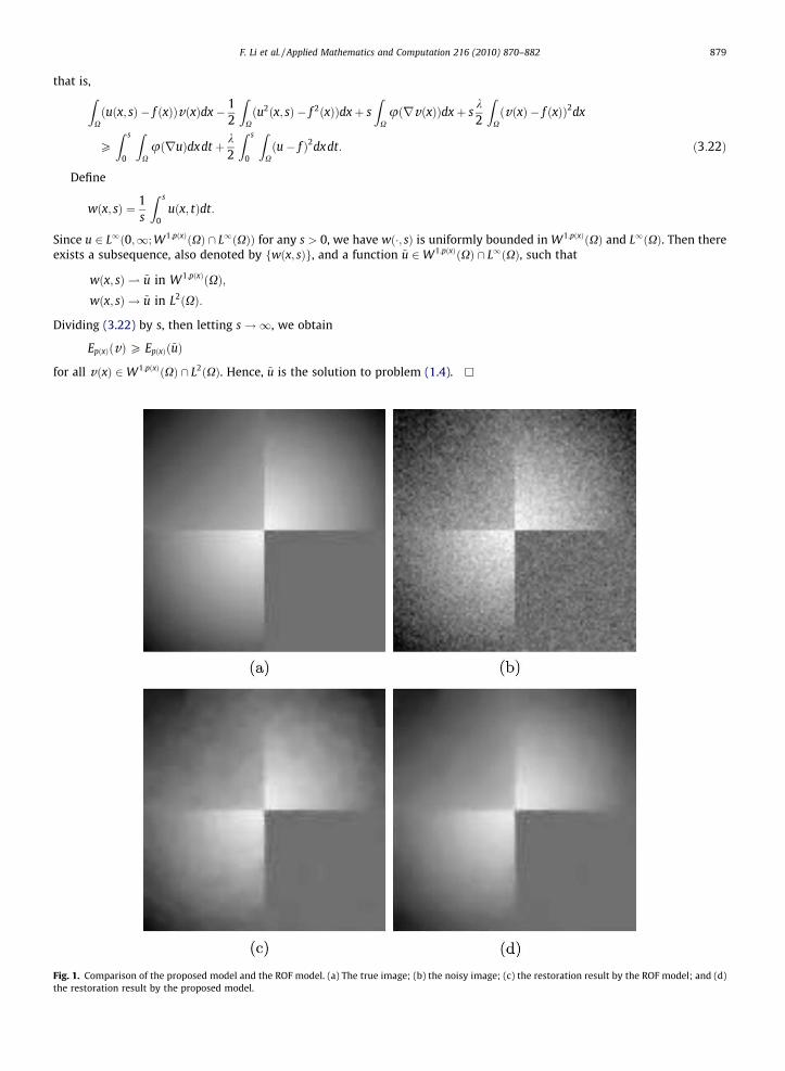
Comparison of the proposed model and the ROF model. (a) The true image; (b) the noisy image; (c) the restoration result by the ROF model; and (d)oration result by the proposed model.


4. Numerical results

We consider dimension n ¼ 2. Suppose the image size is N � N. Set s be the time step and h ¼ 1 be the space step. Letxi ¼ ih; yj ¼ jh; i; j ¼ 0;1; . . . ;N; tn ¼ ns;n ¼ 0;1; . . . ; un

i;j ¼ uðxi; yj; tnÞ; u0ij ¼ f ðxi; yjÞ. Define

Fig. 2.(d) the

ðD�x uÞi;j ¼ �½ui�1;j � ui;j�; ðD�y uÞi;j ¼ �½ui;j�1 � ui;j�;

jðDxuÞi;jj ¼ffiffiffiffiffiffiffiffiffiffiffiffiffiffiffiffiffiffiffiffiffiffiffiffiffiffiffiffiffiffiffiffiffiffiffiffiffiffiffiffiffiffiffiffiffiffiffiffiffiffiffiffiffiffiffiffiffiffiffiffiffiffiffiffiffiffiffiffiffiffiffiffiffiffiffiffiffiffiffiffiffiffiffiffiffiffiffiffiffiffiffiðDþx ðui;jÞÞ2 þ ðm½Dþy ðui;jÞ;D�y ðui;jÞ�Þ2 þ 0:001

q;

jðDyuÞi;jj ¼ffiffiffiffiffiffiffiffiffiffiffiffiffiffiffiffiffiffiffiffiffiffiffiffiffiffiffiffiffiffiffiffiffiffiffiffiffiffiffiffiffiffiffiffiffiffiffiffiffiffiffiffiffiffiffiffiffiffiffiffiffiffiffiffiffiffiffiffiffiffiffiffiffiffiffiffiffiffiffiffiffiffiffiffiffiffiffiffiffiffiffiðDþy ðui;jÞÞ2 þ ðm½Dþx ðui;jÞ;D�x ðui;jÞ�Þ2 þ 0:001

q;

where m½a; b� ¼ sign aþsign b2

� ��minðjaj; jbjÞ. Then the finite difference scheme of the heat flow (3.1)–(3.3) is given by

ukþ1 ¼ uk þ s D�xDþx uk

jDxukj1�g

!þ D�y

Dþy uk

jDyukj1�g

!� kðuk � f Þ

!;

u0 ¼ f ;

where the subscripts i, j are omitted for simplicity. Remark that the Neumann boundary condition (3.2) is implemented byextend the image matrix symmetrically. To illustrate that our model has the advantage of reducing the staircasing effectwhile preserving edges, we run the ROF model as comparison. The numerical scheme of the ROF model is according to [12].

Comparison of the proposed model and the ROF model. (a) A part of Lena image; (b) the noisy image; (c) the restoration result by the ROF model; andrestoration result by the proposed model.

Fig. 3. Comparison of the proposed model and the ROF model. (a) The noisy image; (b) the restoration result by the ROF model; and (c) the restorationresult by the proposed model.

Fig. 4. Comparison of the proposed model and the ROF model. (a) Noisy MRI image of a heart; (b) the restoration result by the ROF model; and (c) therestoration result by the proposed model.


In all the experiments in this paper, the time step is set as 0.05, the fidelity coefficient k is set as 0.01, k ¼ 0:005, andr ¼ 0:5. The stopping criterion of both the ROF model and our model is the relative difference of the restored image shouldsatisfy the following inequality:

kukþ1 � ukk2

kukþ1k2< 10�4:

In Fig. 1, a typical piecewise smooth image is tested. Fig. 1(b) is the noisy version of Fig. 1(a). The restoration results by theROF model and the proposed model are showed in Fig. 1(c) and (d), respectively. We can see in both results that the edges inthe centerlines are preserved. However, in Fig. 1(c) the staircasing effect is obvious in the smooth regions, while in Fig. 1(d)the staircasing effect is successfully reduced.

A part of Lena image is tested in Fig. 2. Fig. 2(b) is the noisy version of Fig. 2(a). Figs. 2(c) and (d) show the restorationresults by the ROF model and the proposed model, respectively. We can see that the proposed model recovers sharp edgesas effectively as the ROF model. Meanwhile, in the smooth regions such as the shoulder, the staircasing effect can be seen inFig. 2(c), while in Fig. 2(d) almost no staircasing effect occurs in these regions such that it seems more natural.

In Fig. 3, we test a character image with smooth background. Fig. 3(a) shows the noisy image. Figs. 3(b) and (c) show therestoration results by the ROF model and the proposed model, respectively. We observe that in both results the edges of thecharacters are preserved. Meanwhile, almost no staircasing effect appears when processed by the proposed model.

We test a medical image in Fig. 4. An MRI image of a heart with noise is showed in Fig. 4(a). Figs. 4(b) and (c) show therestoration results by the ROF model and the proposed model, respectively. The staircasing effect is obvious on the surface ofthe organ in Fig. 4(b), in contrast, almost no staircasing effect occurs in Fig. 4(c) where the organ surface is smooth.

5. Conclusion

In this paper, we have studied a variational exponent ð1 < pðxÞ 6 2Þ functional to recover images based on the models(1.2) and (1.3). The significant difference between our model and (1.3) is that in our model (1.4) pðxÞ can approximate 1


(but larger than 1) while in (1.3) pðxÞwill be equal to 1 in regions with large gradient. However, theoretically, the two modelsare discussed in different spaces. (1.3) is studied in BV space while (1.4) is studied in variable exponent Sobolev space W1;pðxÞ.

The case that includes pðxÞ ¼ 1 is interesting. Some lemmas in Section 3 no longer hold any more. If 1 6 pðxÞ 6 2, otherkind of variable exponent space (not W1;pðxÞ) should be introduced. This will be the future work.

Acknowledgements

This work is partially supported by the National Science Foundation of Shanghai (10ZR1410200), the National ScienceFoundation of China (10901104, 10871126) and the Research Fund for the Doctoral Program of Higher Education(200802691037).

References

[1] P. Blomgren, T.F. Chan, P. Mulet, C. Wong, Total variation image restoration: numerical methods and extensions, in: Proceedings of the 1997 IEEEInternational Conference on Image Processing, vol. III, 1997, pp. 384–387.

[2] E.M. Bollt, R. Chartrand, S. Esedoglu, P. Schultz, K.R. Vixie, Graduated adaptive image denoising: local compromise between total variation and isotropicdiffusion, Adv. Comput. Math. 31 (2009) 61–85.

[3] Y.M. Chen, S. Levine, M. Rao, Variable exponent, linear growth functionals in image restoration, SIAM J. Appl. Math. 66 (2006) 1383–1406.[4] L.C. Evans, Partial Differential Equations, Graduate Studies in Mathematics, vol. 19, A.M.S., Providence, RI, 1998.[5] X.-L. Fan, Q.-H. Zhang, Existence of solutions for p(x)-Laplacian Dirichlet Problem, Nonlinear Anal. 52 (2003) 1843–1852.[6] X.-L. Fan, D. Zhao, On the generalized Orlicz–Sobolev space Wk;pðxÞðXÞ, J. Gansu Edu. College 12 (1998) 1–6.[7] P.A. Hästö, On the existence of minimizers of the variable exponent Dirichlet energy integral, Commun. Pure Appl. Anal. 5 (2006) 415–422.[8] O. Kovác̆ik, J. Rákosník, On spaces LpðxÞ and W1;pðxÞ, Czechoslovak Math. J. 41 (1991) 592–618.[9] O.A. Ladyz̆enskaja, V.A. Solonnikov, N.N. Uralceva, Linear and quasilinear equations of parabolic type, in: S. Smith (Ed.), Translated from the Russian,

Translations of Mathematical Monographs, vol. 23, American Mathematical Society, Providence, R.I., 1967.[10] F.H. Lin, X.P. Yang, Geometric Measure Theory – An Introduction, Advanced Mathematics, International Press, Boston, 2001.[11] M. Nikolova, Weakly constrained minimization: application to the estimation of images and signals involving constant regions, J. Math. Imaging Vis. 21

(2004) 155–175.[12] L.I. Rudin, S. Osher, E. Fatemi, Nonlinear total variation based noise removal algorithms, Physica D 60 (1992) 259–268.[13] M. Sanchón, J.M. Urbano, Entropy solutions for the p(x)-Laplace equation, Trans. Amer. Math. Soc. 361 (2009) 6387–6405.[14] D.M. Strong, T.F. Chan, Edge-preserving and scale-dependent properties of total variation regularization, Inverse Problems 19 (2003) S165–S187.[15] Y.-L. You, W. Xu, A. Tannenbaum, M. Kaveh, Behavioral analysis of anisotropic diffusion in image processing, IEEE Trans. Image Process. 5 (1996) 1539–

1553.[16] X. Zhou, An evolution problem for plastic antiplanar shear, Appl. Math. Optim. 25 (1992) 263–285.

Documents

Variable exponent functionals in image restoration