Embed Size (px)
Citation preview

Variability & Queuing IV

Review• Little’s Law• Basic Queuing Models/Approximations
– M/M/1, M/M/m, G/G/1, G/G/m• Variability
– Quantifying (CV & SCV)– Sources:
• natural• incidental
– setups– breakdowns
• Applications– Performance modeling, “cost” analysis, decision making

Qcalc.xls
• Spreadsheet that contains all the models we’ve discussed
• To use it, you will need to be able to convert parameters given in problem to parameters used in the spreadsheet
• You will have to make sure your units are consistent

“Economic” Analysis of Queues
• Cost of service– fixed cost (equipment, space, etc)– variable cost (materials, wages, etc)
• “Cost” of waiting– opportunity cost of variable “investment”– opportunity cost of delay
• obsolescence, price erosion, lost sales, engineering changes
Textbook Approach
• Hypothesize a “cost of waiting”• Formulate a “total cost” model• Vary waiting cost parameter to see
how it affects total cost
• I’m not crazy about this approach...

You can never know the value of the waiting cost parameter
• But you can observe the impact of waiting time
• My suggestion: vary what you can control, observe the resulting performance, and identify an appropriate “performance target.”

Example, pp. 166-170
• Ra=5, Rs=8• How many servers?
• Number of servers is what you can control; average waiting time is the performance variable of interest

Use Qcalc.xlsWaiting Time vs. # Servers
0
5
10
15
20
0 1 2 3 4 5 6
Number of Servers
Expe
cted
Wai
ting
Tim
e
Target service level

General Strategy
• Minimize cost of service• Subject to service level constraint(s)
• Why do I prefer this to a ‘waiting cost’ model?

Big PictureDescriptive Models•Little’s law•Process flow graph•Process flow chart•From/to matrix
Analytic Models•Queuing•Simulation
Decision Support

Monte Carlo Sampling
And Simulation

Sample data generator
• Inter-arrival times and service times are drawn from exponential distributions.
• Event times are computed from “observations”
• Get a new sample every time the spreadsheet is recalculated

Sampling ProcedureExponential Distribution
0
0.2
0.4
0.6
0.8
1
1.2
0 2 4 6 8 10 12
Time
Dens
ity/C
umul
ativ
e

Sampling Procedure
• Requires “random” numbers in (0, 1)• Requires the inverse of F(x)• F(x) = 1-exp(-λx) = r [random number]• exp(-λx) = 1-r• ln(exp(-λx) ) = -λx = ln(1-r)• x = -(1/λ)ln(1-r) = -(1/λ)ln(r)

0
0.2
0.4
0.6
0.8
1
1.2
0 2 4 6 8 10 12
0.6873
.98 2.35
1. Generate the “random” number2. Find the inter-arrival time that
corresponds to that probability in the cumulative density function
0.9250
Random Numbers
• There are mathematical methods that generate sequences of “pseudo-random” numbers.
• Excel has a function, rand()

MM1Sim.xls
How I generated samples of 1000 jobs for the Norcen
grinder!

How “random” are Excel’s random numbers?

Sample of 1000 Rand() ValuesHistogram of 1000 random numbers
05
101520253035404550
0.000
2532
260.0
6470
4553
0.129
1558
8
0.193
6072
080.2
5805
8535
0.322
5098
630.3
8696
119
0.451
4125
170.5
1586
3845
0.580
3151
720.6
4476
6499
0.709
2178
270.7
7366
9154
0.838
1204
820.9
0257
1809
0.967
0231
36
Bin Ranges
Cou
nt

Chart of 1000 random points in the unit square
0
0.2
0.4
0.6
0.8
1
1.2
0 0.2 0.4 0.6 0.8 1 1.2

Chart of 10000 random points in the unit square
0
0.2
0.4
0.6
0.8
1
1.2
0 0.2 0.4 0.6 0.8 1 1.2

Monte Carlo Sampling
• Traditional name for this method• Very flexible• I can generate as many samples as I
want• I can generate larger or smaller
samples

Monte Carlo sampling is a tool that allows us to create
“synthetic” data. We assumesome distribution for the
random process of interest, and use Monte Carlo sampling to create “observations” of this
random variable. All we need is a distribution function.

Empirical Distributions
• Monte Carlo sampling also works with empirical distributions
• Can use the discrete distribution (the histogram), or
• Can interpolate to get values in between the bin boundaries
• Need the vlookup() function in Excel
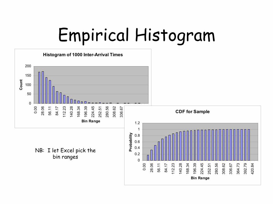
Empirical HistogramHistogram of 1000 Inter-Arrival Times
0
50
100
150
200
0.00
28.0
6
56.1
1
84.1
7
112.
23
140.
28
168.
34
196.
39
224.
45
252.
51
280.
56
308.
62
336.
67
364.
73
392.
79
420.
84
Bin Range
Cou
nt
CDF for Sample
0
0.2
0.40.6
0.8
1
1.2
0.00
28.0
6
56.1
1
84.1
7
112.
23
140.
28
168.
34
196.
39
224.
45
252.
51
280.
56
308.
62
336.
67
364.
73
392.
79
420.
84
Bin Range
Prob
abili
ty
NB: I let Excel pick the bin ranges

Sampling from discrete CDFCDF for Sample
0
0.2
0.40.6
0.8
1
1.20.
00
28.0
6
56.1
1
84.1
7
112.
23
140.
28
168.
34
196.
39
224.
45
252.
51
280.
56
308.
62
336.
67
364.
73
392.
79
420.
84
Bin Range
Prob
abili
ty
70.14
.664
NB: Can use the Excel function vlookup() to do this, but there’s a trick

Using vlookupSearches for a value in the leftmost column of a table, and thenreturns a value in the same row from a column you specify in thetable.
VLOOKUP(lookup_value, table_array, col_index_num, range_lookup)
Lookup_value is the value to be found in the first column of the array. Lookup_value can be a value, a reference, or a text string.
Table_array is the table of information in which data is looked up. Use a reference to a range or a range name, such as Databaseor List.
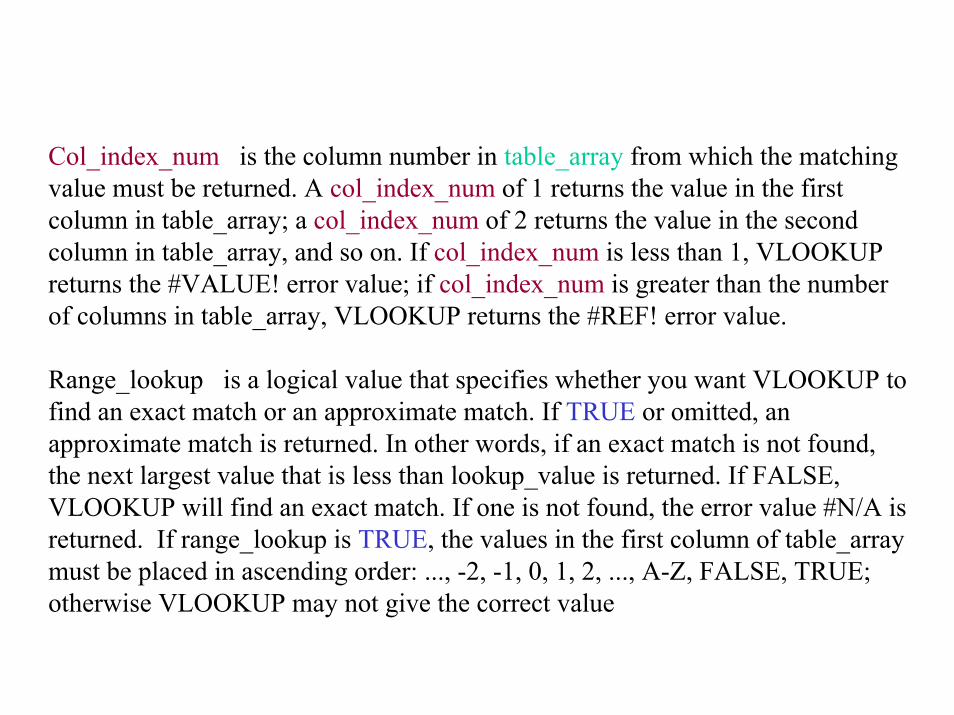
Col_index_num is the column number in table_array from which the matching value must be returned. A col_index_num of 1 returns the value in the first column in table_array; a col_index_num of 2 returns the value in the second column in table_array, and so on. If col_index_num is less than 1, VLOOKUP returns the #VALUE! error value; if col_index_num is greater than the number of columns in table_array, VLOOKUP returns the #REF! error value.
Range_lookup is a logical value that specifies whether you want VLOOKUP to find an exact match or an approximate match. If TRUE or omitted, an approximate match is returned. In other words, if an exact match is not found, the next largest value that is less than lookup_value is returned. If FALSE, VLOOKUP will find an exact match. If one is not found, the error value #N/A is returned. If range_lookup is TRUE, the values in the first column of table_array must be placed in ascending order: ..., -2, -1, 0, 1, 2, ..., A-Z, FALSE, TRUE; otherwise VLOOKUP may not give the correct value

vlookup examples
K L
1 0 14.030062 170 28.058063 342 42.086064 482 56.114075 606 70.142076 697 84.170077 761 98.198078 819 112.2261
VLOOKUP(344, $K$1:$L$31,1,1)=342VLOOKUP(507, $K$1:$L$31,1,1)=482VLOOKUP(600, $K$1:$L$31,1,1)=482
VLOOKUP(750, $K$1:$L$31,2,1)= ?VLOOKUP(800, $K$1:$L$31,2,1)= ?
See the “histograms” tab in MM1Sim.xls, where vlookup is used, both with and without
interpolation

The Trick in Using VLOOKUP
• You have to shift the bin range up one cell, relative to the cum prob, in order to generate the desired target
• See MM1Sim.xls for examples

This works, but ...
• yields only a few unique values• on the other hand, it’s “easy”• we can do a little more work and get
continuous values by interpolating

Interpolating
70.14
56.11
697
606
x
664
X=56.11+ (70.14-56.11)*(664-606)/(697-606) = 65.05

Inter-departure times
• Describe the way jobs are presented to the material handling system, i.e., the “arrival process” for the MHS
• The from/to chart tells the distribution of destinations but not the distribution of inter-arrival times to the MHS

MM1Sim.xlsInter-Departure Times
0
20
40
60
80
100
120
140
160
180
200
0.03
0847
694
26.0
7061
787
52.1
1038
804
78.1
5015
822
104.
1899
284
130.
2296
986
156.
2694
687
182.
3092
389
208.
3490
091
234.
3887
793
260.
4285
494
286.
4683
196
312.
5080
898
338.
5478
6
364.
5876
301
390.
6274
003
Time
Freq
uenc
y
0
0.2
0.4
0.6
0.8
1
1.2
Cum
ulat
ive
Perc
ent

Now Suppose
• There are two kinds of jobs, appearing at random, with equal probability
• One has a service time that is U(12.5, 37.5)
• One has a service time that is U(62.5, 87.5)
• Departures.xls

Inter-Departure Times
0
20
40
60
80
100
120
140
160
180
12.5
0292
165
31.6
8583
38
50.8
6874
596
70.0
5165
811
89.2
3457
027
108.
4174
824
127.
6003
946
146.
7833
067
165.
9662
189
185.
1491
3120
4.33
2043
2
223.
5149
554
242.
6978
675
261.
8807
797
281.
0636
918
300.
2466
04
Time
Freq
uecy
0
0.2
0.4
0.6
0.8
1
1.2
Cum
ulat
ive
Perc
ent

Also ...
• What if we don’t have “unlimited” staging capacity for waiting jobs?
• What if we need more reliable estimates of “departure time”?
• What are the relevant cost factors?• What if …?

We may need analysis tools
With a little more “resolution” than the basic queueing models
provide...

Assignment
• Play with the spreadsheet to get a feel for variability and the impact of increasing utilization
• Modify the spreadsheet to generate a larger sample, and compare the distributions of sample averages for different sample sizes.

Final note on MC sampling
It can be useful for lots of other applications as well. For example, the spreadsheet illustrates the use of MC sampling to estimate the area of a circle. You could use MC sampling to estimate the area of other shapes, even non-geometrical shapes. The key is to define a function that evaluates to “true” or “false” when you substitute in the sampled values.

Be Sure You:
• Read the material on Monte Carlo sampling and simulation in the text
• Look at the spreadsheets--play around with them to make sure you understand how they work.
• Look at the Excel function for generating observations from other distributions, in tools -> data_analysis ->random_number_generation


![[MS-MQSO]: Message Queuing System Overviewdownload.microsoft.com/download/5/0/1/501ED102-E53F-4CE0-AA6B... · This document provides an overview of the Message Queuing System Overview](https://img.pdfslide.us/doc/110x75/5e3dfe16c797d0716a63f4ad/ms-mqso-message-queuing-system-this-document-provides-an-overview-of-the-message.jpg)


![15-744: Computer Networking L-5 Fair Queuing. 2 Fair Queuing Core-stateless Fair queuing Assigned reading [DKS90] Analysis and Simulation of a Fair Queueing](https://img.pdfslide.us/doc/110x75/56649dc65503460f94abad7b/15-744-computer-networking-l-5-fair-queuing-2-fair-queuing-core-stateless.jpg)