SCIENTIFIC NOTE

VARIABILITY AND UNCERTAINTY OF BIOKINETIC MODELPARAMETERS: THE DISCRETE EMPIRICAL BAYESAPPROXIMATIONGuthrie Miller*Los Alamos National Laboratory, Los Alamos, NM, USA

Received March 3 2008, revised May 21 2008, accepted June 10 2008

In the Bayesian approach to internal dosimetry, uncertainty and variability of biokinetic model parameters need to be takeninto account. The discrete empirical Bayes approximation replaces integration over biokinetic model parameters by discretesummation in the evaluation of Bayesian posterior averages using Bayes theorem. The discrete choices of parameters aretaken as best-fit point determinations of model parameters for a study subpopulation with extensive data. A simple heuristicmodel is constructed to numerically and theoretically study this approximation. The heuristic example is the measurement ofheights of a group of people, say from a photograph where measurement uncertainty is significant. A comparison is made ofposterior mean and standard deviation of height after a measurement, (i) using the exact prior describing the distributionof true height in the population and (ii) using the approximate discrete empirical Bayes prior obtained from measurements ofsome study subpopulation.

INTRODUCTION

Internal dosimetry relies on biokinetic models torelate the measured bioassay quantities, for example,urinary excretion, to the imparted internal dose. It iswell recognised that biokinetic model parameters areuncertain and variable in any population of interest.In the Bayesian approach to internal dosimetry(1), bio-kinetic model parameter variability and uncertaintycan be taken into account by averaging over a discreteset of biokinetic models (different choices of modelparameters). This assertion follows from the purelymathematical fact that the integration over biokineticmodel parameters that appears in Bayes theorem canbe approximated by a discrete summation. For thisapproach to be useful in practice, one must decidehow to choose the finite discrete set of biokineticmodels and have some idea of the errors introducedrelative to exact evaluation of the Bayesian integrals.

One always seeks to determine the biokinetic priorprobability distribution as much as possible frommeasurement data. Such data usually take the formof a representative study subpopulation with exten-sive high quality measurements. How then is one touse such a study data set to determine a biokineticprior? A number of approaches are currently beingstudied(2,3). The approach described here is quitesimple and intuitive. Point determinations of

biokinetic parameters are made for each case in thestudy subpopulation using minimum-x2 datafitting(4), where certain key biokinetic parameters arechosen to be variable. These point determinations arethe discrete models that are to be averaged over in theevaluation of posterior probabilities using Bayestheorem. A generalisation of this approach(4) not dis-cussed further here would be to generate somenumber (�1, perhaps on the order of 10–100) alter-nate realisations of the biokinetic parameters foreach study case to represent uncertainty.

As an example, for plutonium using standardInternational Commission on Radiation Protection(ICRP) models, the number of biokinetic parametersis on the order of 50. Even a study subpopulationwith extensive good data is usually not sufficient todetermine all these parameters, so assumptions haveto be made about which parameters are of mostimportance. The problem is simplified by allowingvariations only of these key parameters. The ultimateBayesian method would need to allow all parametersto vary and, using the data from the study subpopu-lation, would determine their joint posterior distri-bution, which is to be used as a prior for other cases.This ultimate statistical approach is many years if notdecades off in the future for cases with many par-ameters, like plutonium using standard ICRP models.

This paper considers a simple heuristic example,the measurement of heights of persons in a particu-lar population. This example is sufficiently simple so*Corresponding author: guthrie@lanl.gov

# The Author 2008. Published by Oxford University Press. All rights reservedThe online version of this article has been published under an open access model. Users are entitled to use, reproduce, disseminate, or display the openaccess version of this article for non-commercial purposes provided that: the original authorship is properly and fully attributed; the Journal and OxfordUniversity Press are attributed as the original place of publication with the correct citation details given; if an article is subsequently reproduced ordisseminated not in its entirety but only in part or as a derivative work this must be clearly indicated. For commercial re-use, please contactjournals.permissions@oxfordjournals.org

Radiation Protection Dosimetry (2008), Vol. 131, No. 3, pp. 394–398 doi:10.1093/rpd/ncn180Advance Access publication 8 August 2008

at Brow

n University on June 19, 2012

http://rpd.oxfordjournals.org/D

ownloaded from

that calculations are easily carried out, yet it is stillinstructive.

THE DISCRETE EMPIRICAL BAYESMETHOD

The discrete empirical Bayes method uses pointdeterminations of biokinetic parameters from arepresentative set of study subpopulations with gooddata from a population to construct a prior prob-ability distribution of biokinetic parameters for thispopulation. There are two sources of uncertainty:(1) inter-individual variability in the population and(ii) measurement uncertainty. The simple empiricalBayes method assumes that variability dominatesmeasurement uncertainty (for the measurementsused to determine the prior). Because the sample ofcases is considered to be representative of the popu-lation being studied as a whole, the empirical-Bayesprior would be an inter-individual variability mixtureof distributions, each component of the mixturecorresponding to one case, for a large sample ofrepresentative cases. There are imagined to be twotypes of measurements: (i) prior-determinationmeasurements of high quality (quality perhaps repre-senting quantity of data for a real-life study subpopu-lation) and (ii) the normal measurements that are tobe used with the empirical Bayes prior to determinethe quantities of interest. A particular study casedetermines a single prior mixture component, which isthe posterior resulting from the prior-determinationmeasurements for that case. This discrete empiricalBayes method merely replaces the posterior distri-bution for each study case with a delta-functiondistribution corresponding to the minimum-x2 deter-mination of biokinetics parameters for that case.

As a simple heuristic example of the discreteempirical Bayes method, it is imagined that it isdesired to determine the heights of a group ofpersons in a situation where measurement uncer-tainty is significant, say when heights are determinedfrom a photograph. In the case of heights ofpersons, there are readily available data(5) that couldbe used to construct a prior probability distributionof heights based on knowledge of the population(e.g. age, sex and ethnicity). Thus, it is imagined thatthere is a known, exactly correct prior. This priordistribution of heights in the population is assumedto be a Gaussian distribution with mean value h0and standard deviation s0. The discrete empiricalprior will be compared with this exact prior.

For the determination of the discrete empiricalBayes prior, it is assumed that the measurementtechnique is known to have a Gaussian likelihoodfunction with standard deviation s. To test the dis-crete empirical Bayes method, a single measurementwith result M and Gaussian-likelihood standarddeviation sm is interpreted using (i) the exact

formula from Bayes theorem, and (ii) the discreteempirical Bayes approximation based on N casesused to determine the prior, and the two interpret-ations compared.

When the distribution of true heights in the popu-lation P(h) is known exactly and this is used asthe prior, Bayes theorem(6) gives the posteriorprobability distribution of true height after themeasurement as

PðhjMÞ ¼ PðMjhÞPðhÞÐPðMjhÞPðhÞdh

; ð1Þ

where P(Mjh) is the probability of obtainingmeasurement result M when the true height is h,assumed to be given by

PðMjhÞ ¼ 1ffiffiffiffiffiffi2pp

smexp � 1

2M � hsm

� �2 !

: ð2Þ

In Bayesian inference, the measurement result M isknown and equation (2), termed the likelihood func-tion, is used to infer the true value of the heightusing Bayes theorem, equation (1).

Because both the prior and the likelihood functionin equation (1) are Gaussian, the posterior given byequation (1) is also Gaussian with mean value (theexact posterior mean height)

hðexactÞ ¼ h0=s20 þM=s2

m

1=s20 þ 1=s2

m

; ð3Þ

and posterior standard deviation

sðexactÞh ¼

ffiffiffiffiffiffiffiffiffiffiffiffiffiffiffiffiffiffiffiffiffiffiffiffiffiffiffi1

1=s20 þ 1=s2

m

s: ð4Þ

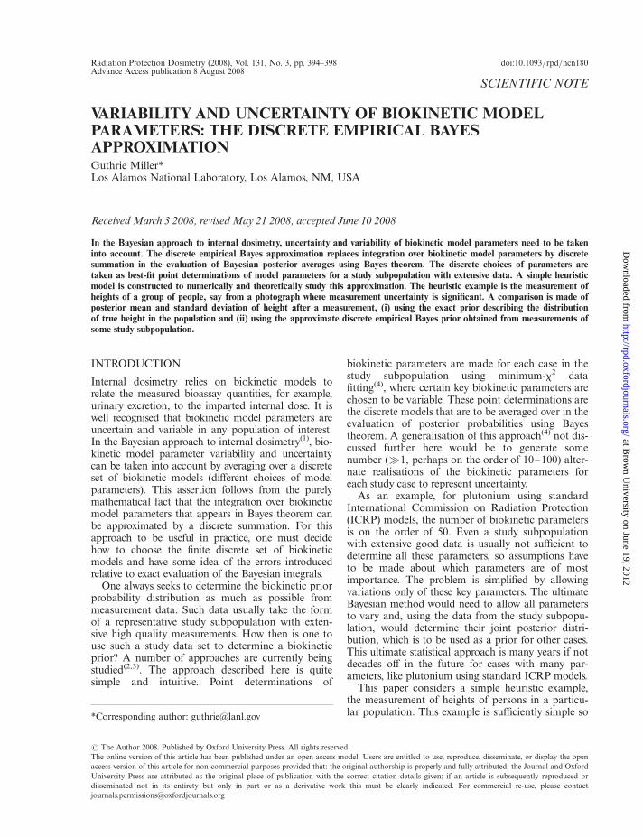
Figure 1 illustrates the situation. The posteriormode (maximum probability point) is pulled awayfrom the likelihood function mode in the directionof the prior mode.

The corresponding plot in terms of cumulativeprobability is shown in Figure 2.

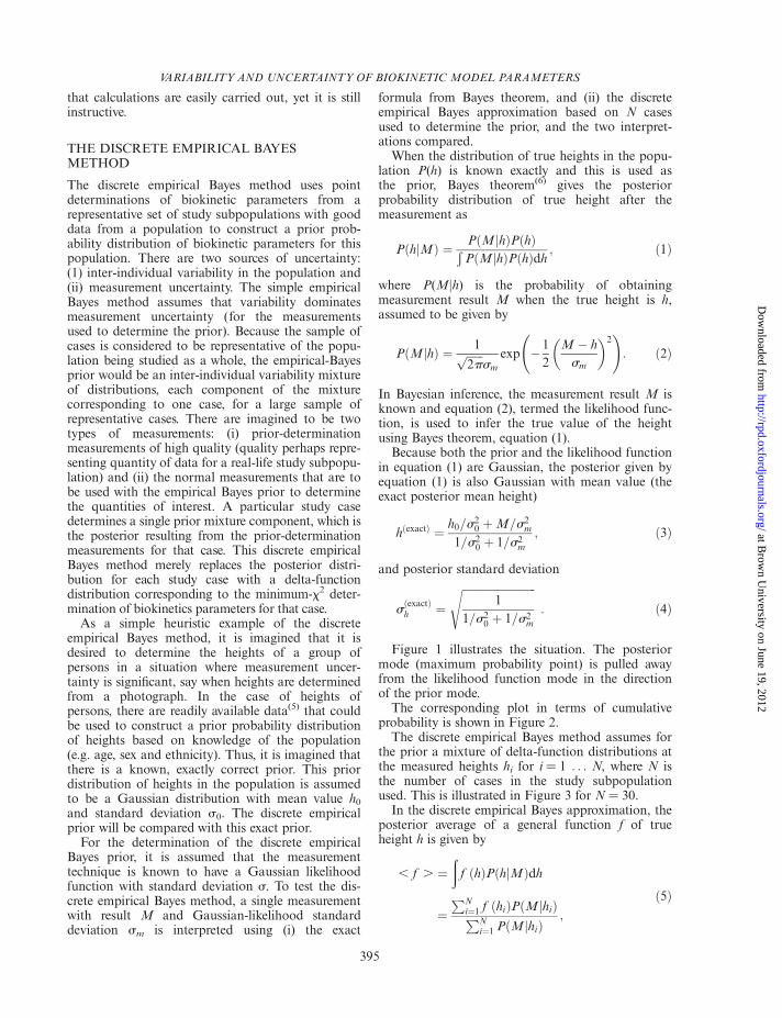
The discrete empirical Bayes method assumes forthe prior a mixture of delta-function distributions atthe measured heights hi for i ¼ 1 . . . N, where N isthe number of cases in the study subpopulationused. This is illustrated in Figure 3 for N ¼ 30.

In the discrete empirical Bayes approximation, theposterior average of a general function f of trueheight h is given by

, f . ¼ð

f ðhÞPðhjMÞdh

¼PN

i¼1 f ðhiÞPðMjhiÞPNi¼1 PðMjhiÞ

;

ð5Þ

VARIABILITY AND UNCERTAINTY OF BIOKINETIC MODEL PARAMETERS

395

at Brow

n University on June 19, 2012

http://rpd.oxfordjournals.org/D

ownloaded from

where hi is the ith measurement result of the Nmeasurements used to determine the prior. Thequantity hi corresponds in this simple example to theminimum-x2 point determination spoken of above. Itis a single best value rather than a distribution. Themeasured heights in equation (5) are those thatwould occur when one randomly selects N cases fromthe population and measures their heights. For thenumerical study, these height measurement resultsare generated from a Gaussian distribution with

mean h0 and standard deviationffiffiffiffiffiffiffiffiffiffiffiffiffiffiffiffis2

0 þ s2q

, where

the measurements used to determine the prior areassumed to have standard deviation s; that is, the dis-tribution of height measurements is broader than thedistribution of true values of height, being affected bymeasurement uncertainty as well as being a measureof variability in the population. In equation (5),P(Mjhi) is the likelihood function corresponding to

the ith study case, given by equation (2). Equation (5)can be used to obtain the posterior mean and stan-dard deviation in the discrete empirical Bayesapproximation by letting the function f (h) ¼ h andf (h) ¼ h2.

A standard diagnostic is x2, given in this case by

x2 ¼ M� , h .

sm

� �2

: ð6Þ

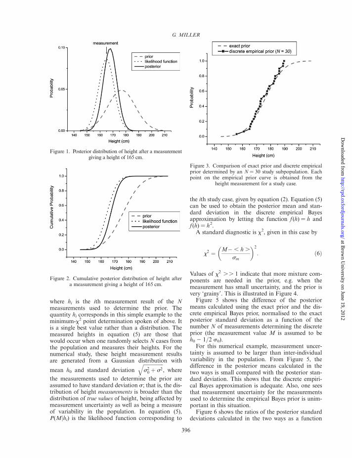
Values of x2 .. 1 indicate that more mixture com-ponents are needed in the prior, e.g. when themeasurement has small uncertainty, and the prior isvery ‘grainy’. This is illustrated in Figure 4.

Figure 5 shows the difference of the posteriormeans calculated using the exact prior and the dis-crete empirical Bayes prior, normalised to the exactposterior standard deviation as a function of thenumber N of measurements determining the discreteprior (the measurement value M is assumed to beh0 2 1/2 s0).

For this numerical example, measurement uncer-tainty is assumed to be larger than inter-individualvariability in the population. From Figure 5, thedifference in the posterior means calculated in thetwo ways is small compared with the posterior stan-dard deviation. This shows that the discrete empiri-cal Bayes approximation is adequate. Also, one seesthat measurement uncertainty for the measurementsused to determine the empirical Bayes prior is unim-portant in this situation.

Figure 6 shows the ratios of the posterior standarddeviations calculated in the two ways as a function

Figure 2. Cumulative posterior distribution of height aftera measurement giving a height of 165 cm.

Figure 1. Posterior distribution of height after a measurementgiving a height of 165 cm.

Figure 3. Comparison of exact prior and discrete empiricalprior determined by an N ¼ 30 study subpopulation. Eachpoint on the empirical prior curve is obtained from the

height measurement for a study case.

G. MILLER

396

at Brow

n University on June 19, 2012

http://rpd.oxfordjournals.org/D

ownloaded from

of the number N of mixture components of the dis-crete prior.One can show that the ratio of standard deviationsin Figure 6 tends toffiffiffiffiffiffiffiffiffiffiffiffiffiffiffiffiffiffiffiffiffiffiffiffiffiffiffiffiffiffiffiffiffiffiffiffiffiffiffiffiffi

1=s20 þ 1=s2

m

1=ðs20 þ s2Þ þ 1=s2

m

s¼ 1:22: ð7Þ

Thus, the discrete empirical Bayes posterior standarddeviation is somewhat larger than it should be. Thiserror goes away if the measurements used to deter-mine the prior have small uncertainty compared

with variability in the population (s much less thans0) or if measurement uncertainty is much smallerthan population variability (sm is much smallerthan s0).

Figure 7 shows x2 as a function of the number Nof measurements determining the discrete prior.

The prior ‘graininess’ problem, which would showup as values of x2 .. 1 for small N does not occur,because of the assumption that measurement uncer-tainty is large compared with population variability.This problem would occur if the height separationof cases constituting the prior was large comparedwith the measurement uncertainty, and none of theheights in the collection of cases constituting theprior was within measurement uncertainty of aheight measurement. The Bayesian ‘universe of pos-sibilities’ would then need to be expanded.

Figure 4. Calculated x2 for height measurements betweentwo prior height measurements of 163 and 175 cm. In thiscase, the measurement uncertainty standard deviation of1 cm is small compared with the separation between priorheights of 175 – 163 ¼ 12 cm, and the values of x2 are

sometimes very large compared with 1.

Figure 5. Difference of posterior means calculated usingthe exact Bayes formula and using the discrete-empirical-

Bayes approximation.

Figure 6. Ratio of posterior standard deviations calculatedusing the exact Bayes formula and using the discrete-

empirical-Bayes approximation.

Figure 7. The quantity x2 as a function of the number ofmeasurements determining the discrete prior.

VARIABILITY AND UNCERTAINTY OF BIOKINETIC MODEL PARAMETERS

397

at Brow

n University on June 19, 2012

http://rpd.oxfordjournals.org/D

ownloaded from

CONCLUSIONS

These types of calculations suggest that the discreteempirical Bayes prior does not significantly bias theposterior mean (Figure 5). The effect of uncertaintyof the measurements determining the prior may beto cause some overestimation of the posterior stan-dard deviation (Figure 6). The x2 diagnostic is usefulin detecting situations where the number of priormixture components N is too small, which mighthappen when the measurement uncertainty is smallcompared with the population variability.

In terms of real-world internal dosimetry, a crudeversion of discrete empirical Bayes has been in use atLos Alamos for many years now(1,7) without evidenceof serious difficulties. In this approach, for 239Puinhalation intakes, the discrete set of biokineticmodels in the biokinetic prior are ICRP-66 type Mand S with particle sizes of 1, 5 and 10 mm AMAD(six models in all). Satisfactory values of x2 areobtained for all cases in the Los Alamos Database(some 30 000 cases). However, for 238Pu, in order tohave satisfactory values of x2, the biokinetic priorneeded to be expanded to include a peculiar ‘delayed-onset’ type of biokinetics(7,8) associated with the‘wing-9’ accident that occurred on 31 July 1971 invol-ving high-fired ceramic material, as well as a variationof type-M behaviour observed in an accident thatoccurred on 16 March 2000. For the Mayak workerstudy(9), a more rigorous application of the discreteempirical Bayes method is being used, with studycases provided by some of the large number of caseswith autopsy tissue data.

ACKNOWLEDGEMENT

The author thanks David Pawel for the idea of usingmeasurement of height as a heuristic example of thediscrete empirical Bayes method.

FUNDING

This work is part of the United States-Russian JointCoordinating Committee for Radiation EffectsResearch (JCCRER) Project 2.5 and is funded

under a Cooperative Agreement with the UnitedStates Department of Energy Office of InternationalHealth Programs (HS-14), Health Safety andSecurity Division (HSS). Funding to pay the OpenAccess publication charges for this article was pro-vided by the United States Department of Energycontract for the management and operation of LosAlamos National Laboratory.

REFERENCES

1. Miller, G., Martz, H. F., Little, T. and Guilmette, R.Bayesian internal dosimetry calculations using Markovchain Monte Carlo. Radiat. Prot. Dosim. 98, 191–198(2002).

2. Puncher, M. and Birchall, A. Estimating uncertainty oninternal dose assessments. Radiat. Prot. Dosim. 127,544–547 (2007).

3. Miller, G., Melo, D., Martz, H. and Bertelli, L. Anempirical multivariate lognormal distribution representinguncertainty of biokinetic parameters for 137Cs. Radiat.Prot. Dosim. 131(2), 198–211 (2008).

4. Miller, G., Bertelli, L. and Guilmette, R. IMPDOS(IMProved DOSimetry and risk assessment for pluto-nium-induced diseases)—internal dosimetry softwaretools developed for the Mayak worker study. Radiat.Prot. Dosim. 131(3), 308–315 (2008).

5. McDowell, M. A., Fryar, C. D., Hirsch, R. and Ogden,C. L. Anthropometric Reference Data for Children andAdults: U.S. Population, 1999–2002. Advance Datafrom Vital and Health Statistics. Centers for DiseaseControl, number 361, 7 July (2005).

6. Miller, G., Inkret, W. C., Schillaci, M. E., Martz, H. F.and Little, T. T. Analyzing bioassay data using Bayesianmethods—a primer. Health Phys. 78, 598–613 (2000).

7. Miller, G., Inkret, W. C. and Martz, H. F. Internaldosimetry intake estimation using Bayesian methods.Radiat. Prot. Dosim. 82(1), 5–17 (1999).

8. James, A. C., Filipy, R. E, Russell, J. J. and Mcinroy, J. F.USTUR Case 0259 whole body donation: a comprehensivetest of the current ICRP models for the behavior ofinhaled 238PuO2 ceramic particles. Health Phys. 84(1),2–33 (2003).

9. Romanov, S. A., Vasilenko, E. K. and Khokhryakov,J. P. Studies on the Mayak nuclear workers: dosimetry.Radiat. Environ. Biophys. 41, 23–28 (2002).

G. MILLER

398

at Brow

n University on June 19, 2012

http://rpd.oxfordjournals.org/D

ownloaded from