Embed Size (px)
Citation preview
HAL Id: hal-00296070https://hal.archives-ouvertes.fr/hal-00296070
Submitted on 31 Oct 2006
HAL is a multi-disciplinary open accessarchive for the deposit and dissemination of sci-entific research documents, whether they are pub-lished or not. The documents may come fromteaching and research institutions in France orabroad, or from public or private research centers.
L’archive ouverte pluridisciplinaire HAL, estdestinée au dépôt et à la diffusion de documentsscientifiques de niveau recherche, publiés ou non,émanant des établissements d’enseignement et derecherche français ou étrangers, des laboratoirespublics ou privés.
Variability and trends in total and vertically resolvedstratospheric ozone based on the CATO ozone data set
D. Brunner, J. Staehelin, J. A. Maeder, I. Wohltmann, G. E. Bodeker
To cite this version:D. Brunner, J. Staehelin, J. A. Maeder, I. Wohltmann, G. E. Bodeker. Variability and trends intotal and vertically resolved stratospheric ozone based on the CATO ozone data set. AtmosphericChemistry and Physics, European Geosciences Union, 2006, 6 (12), pp.4985-5008. �hal-00296070�
Atmos. Chem. Phys., 6, 4985–5008, 2006www.atmos-chem-phys.net/6/4985/2006/© Author(s) 2006. This work is licensedunder a Creative Commons License.
AtmosphericChemistry
and Physics
Variability and trends in total and vertically resolved stratosphericozone based on the CATO ozone data set
D. Brunner1,*, J. Staehelin1, J. A. Maeder1, I. Wohltmann2, and G. E. Bodeker3
1Institute for Atmospheric and Climate Science, ETH Zurich, Switzerland2Alfred Wegner Institute, Potsdam, Germany3National Institute of Water and Atmospheric Research (NIWA), New Zealand* now at: Empa, Swiss Federal Laboratories for Materials Testing and Research, Dubendorf, Switzerland
Received: 22 June 2006 – Published in Atmos. Chem. Phys. Discuss.: 12 July 2006Revised: 25 October 2006 – Accepted: 27 October 2006 – Published: 31 October 2006
Abstract. Trends in ozone columns and vertical distributionswere calculated for the period 1979–2004 based on the ozonedata set CATO (Candidoz Assimilated Three-dimensionalOzone) using a multiple linear regression model. CATO hasbeen reconstructed from TOMS, GOME and SBUV total col-umn ozone observations in an equivalent latitude and poten-tial temperature framework and offers a pole to pole coverageof the stratosphere on 15 potential temperature levels. Theregression model includes explanatory variables describingthe influence of the quasi-biennial oscillation (QBO), vol-canic eruptions, the solar cycle, the Brewer-Dobson circu-lation, Arctic ozone depletion, and the increase in strato-spheric chlorine. The effects of displacements of the polarvortex and jet streams due to planetary waves, which maysignificantly affect trends at a given geographical latitude,are eliminated in the equivalent latitude framework. TheQBO shows a strong signal throughout most of the lowerstratosphere with peak amplitudes in the tropics of the or-der of 10–20% (peak to valley). The eruption of Pinatuboled to annual mean ozone reductions of 15–25% betweenthe tropopause and 23 km in northern mid-latitudes and tosimilar percentage changes in the southern hemisphere butconcentrated at altitudes below 17 km. Stratospheric ozoneis elevated over a broad latitude range by up to 5% duringsolar maximum compared to solar minimum, the largest in-crease being observed around 30 km. This is at a lower alti-tude than reported previously, and no negative signal is foundin the tropical lower stratosphere. The Brewer-Dobson circu-lation shows a dominant contribution to interannual variabil-ity at both high and low latitudes and accounts for some ofthe ozone increase seen in the northern hemisphere since themid-1990s. Arctic ozone depletion significantly affects thehigh northern latitudes between January and March and ex-
Correspondence to:D. Brunner([email protected])
tends its influence to the mid-latitudes during later months.The vertical distribution of the ozone trend shows distinctnegative trends at about 18 km in the lower stratosphere withlargest declines over the poles, and above 35 km in the upperstratosphere. A narrow band of large negative trends extendsinto the tropical lower stratosphere. Assuming that the ob-served negative trend before 1995 continued to 2004 cannotexplain the ozone changes since 1996. A model account-ing for recent changes in equivalent effective stratosphericchlorine, aerosols and Eliassen-Palm flux, on the other hand,closely tracks ozone changes since 1995.
1 Introduction
Anthropogenic stratospheric ozone depletion has been dis-cussed since the early 1970s (Crutzen, 1970; Johnston, 1971;Molina and Rowland, 1974; Stolarski and Cicerone, 1974).In 1985 the Antarctic ozone hole was detected (Farman et al.,1985) and in 1988 significant winter time decreases were firstdocumented for northern mid-latitudes from ground-basedmeasurements and later confirmed by satellite observations(Stolarski et al., 1991). Polar and mid-latitude trends weresubsequently reported in many studies. For an overview seeStaehelin et al.(2001); World Meteorological Organization(2003).
During the 1990s a number of studies provided evidencethat part of the observed trends can be attributed to processesother than anthropogenic ozone depletion. Such processesincluded decadal scale climate variability related to the NorthAtlantic Oscillation (NAO) or Arctic Oscillation (e.g.Ap-penzeller et al., 2000), tropopause altitude (Steinbrecht et al.,1998), and changes in the strength of the Brewer-Dobson cir-culation (Fusco and Salby, 1999; Hadjinicolaou et al., 2002).These factors were found to affect the trends in addition to
Published by Copernicus GmbH on behalf of the European Geosciences Union.
4986 D. Brunner et al.: Vertical distribution of ozone trends
the solar cycle, the quasi-biennial oscillation (QBO) and vol-canic eruptions which had been appreciated already in pre-vious assessments of stratospheric ozone depletion (WorldMeteorological Organization, 1995).
As consequence of the Montreal Protocol and its amend-ments the emissions of anthropogenic ozone depleting sub-stances (ODSs) decreased. According to the temporal evo-lution of ODSs in the stratosphere, chemical ozone deple-tion probably reached a maximum around the late 1990s andslowly decreased thereafter. Therefore, the discussion startedwhether the effect of the Montreal Protocol on the ozonelayer can already be identified in the present observations(Weatherhead et al., 2000; Reinsel et al., 2002; Weatherheadand Andersen, 2006). Newchurch et al.(2003) reported onfirst signs of recovery analyzing upper stratospheric ozonetrends whileReinsel et al.(2005) reported that the lineartrend in total column ozone had changed significantly beyond1996 poleward of 40◦. Identifying ozone recovery requiresboth detection of a positive change in ozone tendency aswell as attribution of that change to decreasing ODSs. Ques-tions remain whether all other factors influencing ozone suchas solar cycle or planetary wave forcing were properly ac-counted for in these studies (Steinbrecht et al., 2004; Dhomseet al., 2006). An important problem in all trend studies usingsatellite data arises from the fact that the ozone time seriesavailable for fitting a statistical model are relatively short incomparison to the timescales of variability of some of the ex-planatory variables. This is additionally complicated by cor-relations among these variables which limits our ability toseparate different effects (Solomon et al., 1996; Salby et al.,1997). Extending the time series out to 2004 now allows fora better separation between solar cycle, volcanic eruptionsand QBO effects. Unlike the previous two solar cycles thelatest one (no. 23) was not synchronized with a major vol-canic eruption and the QBO was in opposite phase duringsolar maximum than previously.
In this study we present the results of a multiple linearregression analysis applied to the quasi-3-D ozone data setCATO (CANDIDOZ Assimilated Three-dimensional Ozone;CANDIDOZ is the EU project ”Chemical and Dynamical In-fluences on Decadal Ozone Change”) (Brunner et al., 2006).In CATO the stratospheric ozone distribution is representedin an equivalent latitude – potential temperature coordinatesystem which has the advantage that it closely follows thecontours of a passive tracer which are distorted by planetarywaves (Schoeberl et al., 1989). Sharp gradients e.g. acrossthe edge of the polar vortex are much better preserved inthis coordinate system than in a standard zonal mean view(Bodeker et al., 2001). In addition, an important part ofdynamical variability associated with planetary waves andmeridional displacements of the vortex is efficiently removedin this framework. These effects not only account for a largefraction of the variability in total ozone observations but alsocontribute to long-term trends in a given geographical lat-
itude band as demonstrated by Wohltmann et al. (2006)1.Since CATO was reconstructed from satellite total ozonemeasurements it provides a unique view of the vertical dis-tribution of stratospheric ozone that is fully consistent withthe total columns. It extends from pole to pole and currentlycovers the period 1979 to 2004 without gaps.
So far only few satellite-based studies are available onlong-term ozone trends in the lower stratosphere where thebulk of ozone resides. However, knowledge of the verti-cal distribution of the trends is essential as it provides ad-ditional insight into the processes governing stratosphericozone. Most previous studies were restricted to altitudeshigher than 20 km due to limitations in profile retrievals fromSAGE (particularly SAGE I) and SBUV which were addi-tionally complicated during periods of enhanced volcanicaerosol. Wang et al.(2002) presented an improved algo-rithm for SAGE II retrievals below 20 km which allowedcalculating ozone trends down to the tropopause for the pe-riod 1984 to 1999. In an earlier study byRandel and Wu(1999) total column data from TOMS were combined withSAGE I/II profile data to calculate the residual amount be-tween the tropopause and 20 km altitude. The present studycomplements these analyzes as it is based on a completelyindependent data set which is more complete in terms of tem-poral and spatial coverage.
Section2.1presents an overview of the CATO data set in-cluding a comparison of time series at different levels in thestratosphere with independent observations. CATO has beendescribed in detail inBrunner et al.(2006). The statisticalmodel is described in Sect.2.2. Results of the regressionanalysis are then shown in Sect.3 both for total ozone andthe corresponding vertical distribution. We highlight the in-fluence of the QBO, solar cycle, volcanic eruptions, plane-tary wave forcing, and polar ozone depletion, and analyzethe trend attributable to the anthropogenic release of ODSs.Finally, in Sect.3.3 we study the recent evolution of ozoneand show that since 1996 there has been a statistically signif-icant change in ozone trend. By using the regression modelto attribute these recent changes to the explanatory variablesincluded in the model, we show to what extent these changesresult from changes in stratospheric ODSs concentrationsand hence to what extent these changes can be interpretedas a sign of ozone recovery.
2 Data and methods
2.1 Reconstructed ozone data set CATO
CATO is a statistically reconstructed data set describing thevertical distribution of ozone in the stratosphere and the hor-izontal distribution of residual ozone columns in the tropo-
1Wohltmann, I., Lehmann, R., Rex, M., Brunner, D., and Mader,J. A.: A process-oriented regression model for column ozone, J.Geophys. Res., submitted, 2006.
Atmos. Chem. Phys., 6, 4985–5008, 2006 www.atmos-chem-phys.net/6/4985/2006/

D. Brunner et al.: Vertical distribution of ozone trends 4987
(a) Mid-latitude anomalies at 40 hPa/22 km
(b) Mid-latitude anomalies at 120 hPa/15 km
(c) Tropical anomalies at 30 hPa/24 km
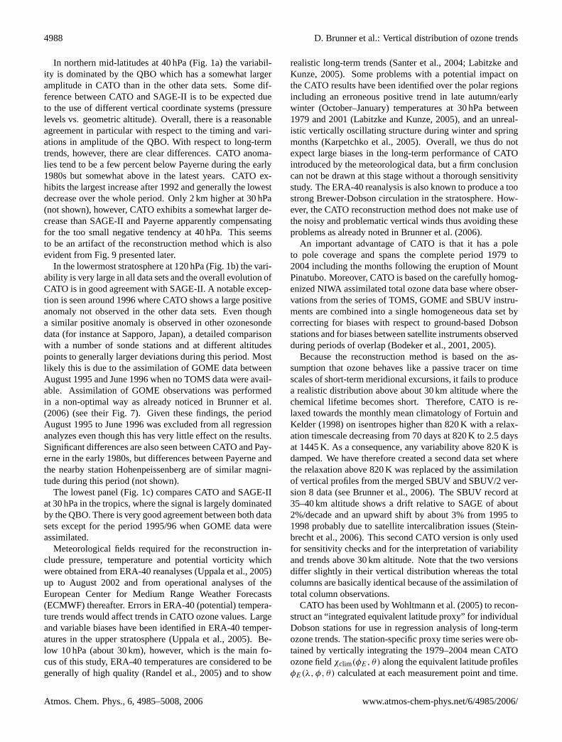
Fig. 1. Time series of normalized monthly ozone anomalies (with respect to the 1985–2004 monthly means) from CATO, Payerne ozoneson-des, and SAGE-II. The thin black lines are the CATO monthly mean anomalies, the thick black lines are 12-month running means throughthese data. For Payerne (blue) and SAGE-II (red) only the running means are shown. Panels (a) and (b) are for northern mid-latitudes. Here,CATO data are mean values over 42◦ to 48◦ N equivalent latitude. SAGE-II are averages over 40◦ to 50◦ N geographical latitude. The stationPayerne, Switzerland, is at 47◦ N. (a) Anomalies at 40 hPa (SAGE-II data at 22 km).(b) Anomalies at 120 hPa (SAGE-II at 15 km).(c)Tropical anomalies at 30 hPa (SAGE-II at 24 km). Here, both CATO and SAGE-II data are 6◦ S to 6◦ N averages.
sphere. It currently covers the period January 1979 to De-cember 2004. The tropospheric columns are represented ingeographical longitude (λ) and latitude (φ) (with 10◦
×6◦
resolution) and the stratospheric distribution in equivalentlatitude (φE) and potential temperature (θ ) coordinates (6◦
horizontal resolution and 15 potential temperature levels be-tween 326 K and 1445 K). The reconstruction is based oncombining satellite total ozone observations with meteoro-logical information on short-term meridional excursions ofair masses due to isentropic transport using a data assimila-tion approach. The method is described in detail inBrunneret al.(2006).
In that paper it was shown that CATO agrees reasonablywell with observations from ozonesondes and HALOE in-cluding a realistic description of seasonal and interannualvariability. Significant deviations from observed profileswere found at high polar latitudes as well as in the trop-ical lower stratosphere. However, these comparisons only
covered data from a few years and therefore did not pro-vide any evidence that CATO is able to reproduce actualchanges in vertical ozone over the whole time period. Fig-ure 1 therefore compares time series of deseasonalized andnormalized (with respect to the 1985–2004 monthly means)monthly ozone anomalies from CATO with the correspond-ing anomalies from a selected ozonesonde station (Payerne,Switzerland, 47◦ N, 7◦ E) and from the Stratospheric Aerosoland Gas Experiment SAGE-II (version 6.2) (Wang et al.,2002). For SAGE-II (thick red lines) and Payerne (thickblue) only 12-month running means are shown for better vis-ibility. For CATO (thick black), additionally the individualmonthly anomalies are presented (thin black). SAGE-II dataduring the first three years after eruption of Mount Pinatuboin June 1991 were affected by the enhanced volcanic aerosoland therefore excluded. Note that CATO data are mean val-ues for a given equivalent latitude band whereas SAGE-II arezonal means in geographical coordinates.
www.atmos-chem-phys.net/6/4985/2006/ Atmos. Chem. Phys., 6, 4985–5008, 2006
4988 D. Brunner et al.: Vertical distribution of ozone trends
In northern mid-latitudes at 40 hPa (Fig.1a) the variabil-ity is dominated by the QBO which has a somewhat largeramplitude in CATO than in the other data sets. Some dif-ference between CATO and SAGE-II is to be expected dueto the use of different vertical coordinate systems (pressurelevels vs. geometric altitude). Overall, there is a reasonableagreement in particular with respect to the timing and vari-ations in amplitude of the QBO. With respect to long-termtrends, however, there are clear differences. CATO anoma-lies tend to be a few percent below Payerne during the early1980s but somewhat above in the latest years. CATO ex-hibits the largest increase after 1992 and generally the lowestdecrease over the whole period. Only 2 km higher at 30 hPa(not shown), however, CATO exhibits a somewhat larger de-crease than SAGE-II and Payerne apparently compensatingfor the too small negative tendency at 40 hPa. This seemsto be an artifact of the reconstruction method which is alsoevident from Fig.9 presented later.
In the lowermost stratosphere at 120 hPa (Fig.1b) the vari-ability is very large in all data sets and the overall evolution ofCATO is in good agreement with SAGE-II. A notable excep-tion is seen around 1996 where CATO shows a large positiveanomaly not observed in the other data sets. Even thougha similar positive anomaly is observed in other ozonesondedata (for instance at Sapporo, Japan), a detailed comparisonwith a number of sonde stations and at different altitudespoints to generally larger deviations during this period. Mostlikely this is due to the assimilation of GOME data betweenAugust 1995 and June 1996 when no TOMS data were avail-able. Assimilation of GOME observations was performedin a non-optimal way as already noticed inBrunner et al.(2006) (see their Fig. 7). Given these findings, the periodAugust 1995 to June 1996 was excluded from all regressionanalyzes even though this has very little effect on the results.Significant differences are also seen between CATO and Pay-erne in the early 1980s, but differences between Payerne andthe nearby station Hohenpeissenberg are of similar magni-tude during this period (not shown).
The lowest panel (Fig.1c) compares CATO and SAGE-IIat 30 hPa in the tropics, where the signal is largely dominatedby the QBO. There is very good agreement between both datasets except for the period 1995/96 when GOME data wereassimilated.
Meteorological fields required for the reconstruction in-clude pressure, temperature and potential vorticity whichwere obtained from ERA-40 reanalyses (Uppala et al., 2005)up to August 2002 and from operational analyses of theEuropean Center for Medium Range Weather Forecasts(ECMWF) thereafter. Errors in ERA-40 (potential) tempera-ture trends would affect trends in CATO ozone values. Largeand variable biases have been identified in ERA-40 temper-atures in the upper stratosphere (Uppala et al., 2005). Be-low 10 hPa (about 30 km), however, which is the main fo-cus of this study, ERA-40 temperatures are considered to begenerally of high quality (Randel et al., 2005) and to show
realistic long-term trends (Santer et al., 2004; Labitzke andKunze, 2005). Some problems with a potential impact onthe CATO results have been identified over the polar regionsincluding an erroneous positive trend in late autumn/earlywinter (October–January) temperatures at 30 hPa between1979 and 2001 (Labitzke and Kunze, 2005), and an unreal-istic vertically oscillating structure during winter and springmonths (Karpetchko et al., 2005). Overall, we thus do notexpect large biases in the long-term performance of CATOintroduced by the meteorological data, but a firm conclusioncan not be drawn at this stage without a thorough sensitivitystudy. The ERA-40 reanalysis is also known to produce a toostrong Brewer-Dobson circulation in the stratosphere. How-ever, the CATO reconstruction method does not make use ofthe noisy and problematic vertical winds thus avoiding theseproblems as already noted inBrunner et al.(2006).
An important advantage of CATO is that it has a poleto pole coverage and spans the complete period 1979 to2004 including the months following the eruption of MountPinatubo. Moreover, CATO is based on the carefully homog-enized NIWA assimilated total ozone data base where obser-vations from the series of TOMS, GOME and SBUV instru-ments are combined into a single homogeneous data set bycorrecting for biases with respect to ground-based Dobsonstations and for biases between satellite instruments observedduring periods of overlap (Bodeker et al., 2001, 2005).
Because the reconstruction method is based on the as-sumption that ozone behaves like a passive tracer on timescales of short-term meridional excursions, it fails to producea realistic distribution above about 30 km altitude where thechemical lifetime becomes short. Therefore, CATO is re-laxed towards the monthly mean climatology ofFortuin andKelder (1998) on isentropes higher than 820 K with a relax-ation timescale decreasing from 70 days at 820 K to 2.5 daysat 1445 K. As a consequence, any variability above 820 K isdamped. We have therefore created a second data set wherethe relaxation above 820 K was replaced by the assimilationof vertical profiles from the merged SBUV and SBUV/2 ver-sion 8 data (seeBrunner et al., 2006). The SBUV record at35–40 km altitude shows a drift relative to SAGE of about2%/decade and an upward shift by about 3% from 1995 to1998 probably due to satellite intercalibration issues (Stein-brecht et al., 2006). This second CATO version is only usedfor sensitivity checks and for the interpretation of variabilityand trends above 30 km altitude. Note that the two versionsdiffer slightly in their vertical distribution whereas the totalcolumns are basically identical because of the assimilation oftotal column observations.
CATO has been used byWohltmann et al.(2005) to recon-struct an “integrated equivalent latitude proxy” for individualDobson stations for use in regression analysis of long-termozone trends. The station-specific proxy time series were ob-tained by vertically integrating the 1979–2004 mean CATOozone fieldχclim(φE, θ) along the equivalent latitude profilesφE(λ, φ, θ) calculated at each measurement point and time.
Atmos. Chem. Phys., 6, 4985–5008, 2006 www.atmos-chem-phys.net/6/4985/2006/
D. Brunner et al.: Vertical distribution of ozone trends 4989
Wohltmann et al. (2006)1 demonstrated that this proxy is ableto explain a large part of total ozone variability measured atthese stations.
2.2 Regression model
The set of explanatory variables (or proxies) chosen for theregression model describes the influence of the solar cycle,the QBO, stratospheric aerosol loading following volcaniceruptions, the strength of the Brewer-Dobson circulation, andthe anthropogenic impact on ozone through release of ozonedepleting substances (ODSs). A linear response of ozone tochanges in these variables is assumed though the responseis allowed to be different for different months of the year.The proxies are selected to model as closely as possible themost relevant processes influencing stratospheric ozone vari-ability. A more detailed motivation for the choice of vari-ables we use here is given in the companion paper by Wohlt-mann et al. (2006)1. Note that in contrast to other trend stud-ies the influence of various climate modes such as NAO orthe El Nino - Southern Oscillation are not included explic-itly. NAO and other climate modes may change the positionof troughs and ridges of planetary waves and hence modu-late the altitude of the tropopause (Appenzeller et al., 2000;Weiss et al., 2001) and invoke meridional advection of ozonefrom regions of higher or lower climatological mean concen-trations (Koch et al., 2002). While this may explain a sig-nificant fraction of ozone variability at a given point on theglobe, much of these effects are eliminated when adoptingan equivalent latitude and potential temperature framework(cf. Wohltmann et al., 2005) which is the approach followedhere. In addition, NAO influences the propagation of wavesinto the stratosphere and hence the deposition of wave mo-mentum driving the Brewer-Dobson circulation (Rind et al.,2005). This further affects the polar vortex which is strongerwhen the NAO is in a positive phase (Schnadt and Dameris,2003). These effects are again accounted for, at least quali-tatively, by including Eliassen-Palm (EP) flux as a proxy forthe Brewer-Dobson circulation (Fusco and Salby, 1999) andthe volume of polar stratospheric clouds (PSC) to describeArctic ozone loss (Rex et al., 2004). The setup of the re-gression model is similar to that byStolarski et al.(1991)or Ziemke et al.(1997) and is formulated in one of the twofollowing forms
Y (t) = a + b · EESC(t) +
N∑j=1
cj · Xj (t) + ε(t) (1)
Y (t) = a + b · t +
N∑j=1
cj · Xj (t) + ε(t) (2)
EESC(t): time series of equivalent effectivestratospheric chlorine
t : number of months since start of record(t=1 for January 1979), used in alternative
model instead ofEESC.Y (t): target variable, monthly mean total ozone column
or ozone partial pressure in montht
a: seasonally varying intercept (offset) of the ozonetime series
b: seasonally varying EESC or trend coefficientXj (t): time series of explanatory variablej (j=1,..,N)cj : seasonally varying coefficients describing the
influence of explanatory variablejN : Number of explanatory variables in addition to
seasonal offset and trend componentsε(t): residual variations not described by the model
Unless we only consider annual mean effects, the regres-sion coefficientsa, b and cj are allowed to depend on themonth of the year. This time dependence is modelled by 12-month and 6-month sine and cosine harmonic series. Thetime dependence of the coefficientscj is thus given by
cj (t) = cj,1 +∑2
k=1 [cj,2k · cos(2πkt/12) +
cj,2k+1 · sin(2πkt/12)] (3)
and the same formula is applied to coefficientsa andb. Thus,usually 5 coefficients need to be estimated for a single proxytime series to account for the fact that the response of ozoneto changes in the proxy may vary with season. Because ofthe small seasonal variation that was found for the influenceof solar effects, only 3 coefficients were used to represent thesolar cycle.
The linear regression model was applied to (i) time se-ries of monthly mean total ozone at 30 discrete equivalentlatitudes (at 6◦ resolution) and (ii) to monthly mean strato-spheric ozone fields as a function of equivalent latitude (sameresolution as total ozone) and pressure. For the latter theCATO fields were interpolated from the native 15 isentropiclevels onto 14 discrete pressure levels (190, 120, 90, 60, 40,30, 20, 15, 10, 7, 5, 3.5, 2.5, 1.5 hPa). Because stratospherictemperatures have a trend on their own, ozone trends on isen-tropes are not identical to trends on pressure levels. We preferthe representation on pressure levels to be compatible withother trend studies. For the analysis of vertical ozone vari-ability only annual mean effects are usually considered here.In this case no harmonic expansion is applied except to theseasonal offseta.
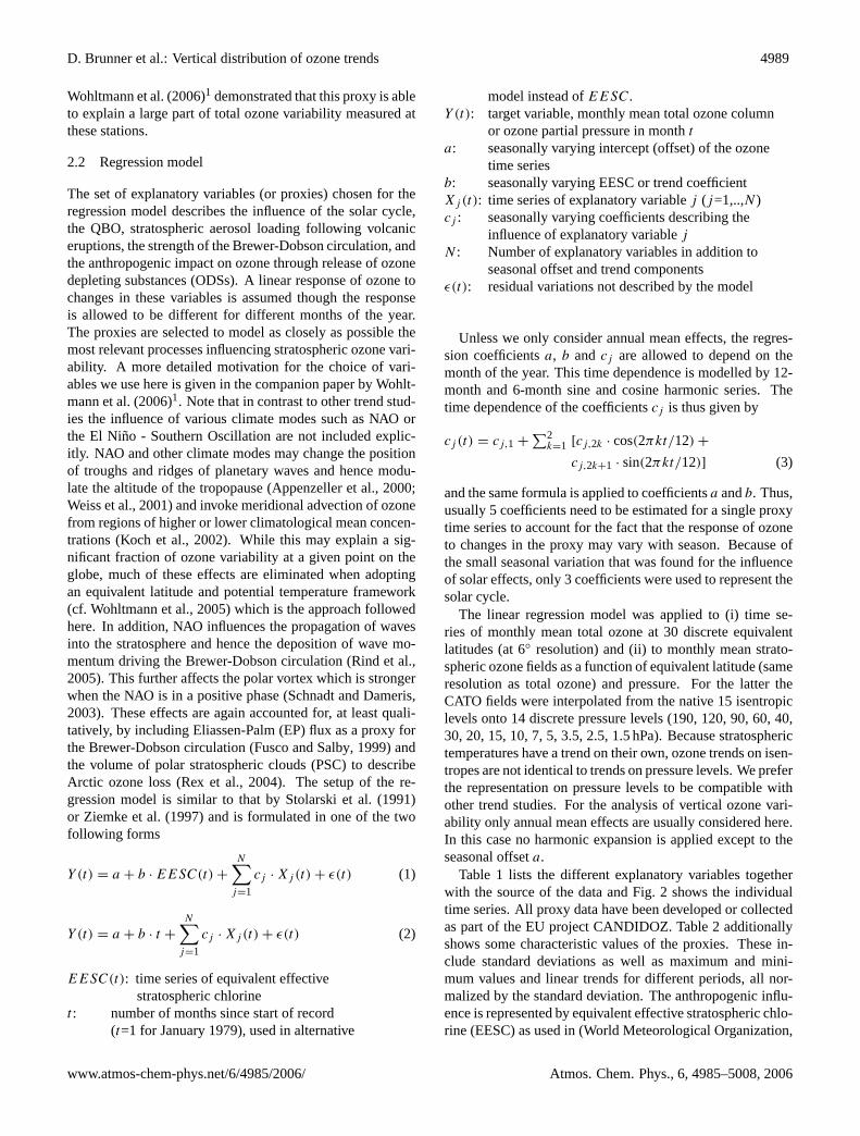
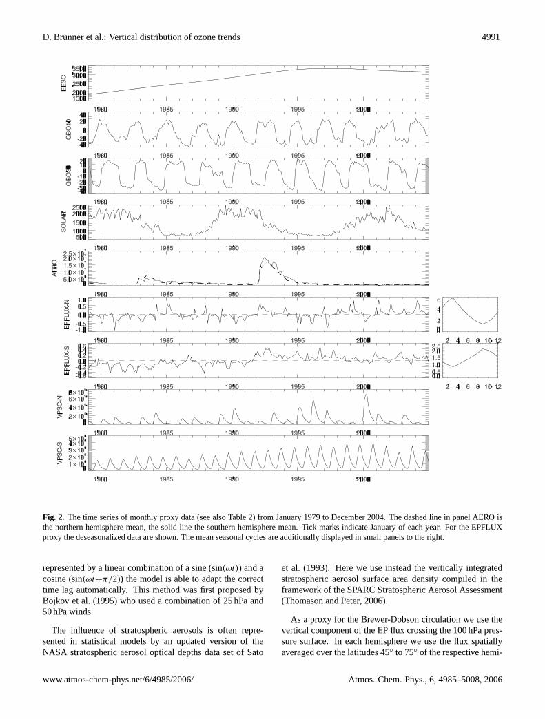
Table 1 lists the different explanatory variables togetherwith the source of the data and Fig.2 shows the individualtime series. All proxy data have been developed or collectedas part of the EU project CANDIDOZ. Table2 additionallyshows some characteristic values of the proxies. These in-clude standard deviations as well as maximum and mini-mum values and linear trends for different periods, all nor-malized by the standard deviation. The anthropogenic influ-ence is represented by equivalent effective stratospheric chlo-rine (EESC) as used in (World Meteorological Organization,
www.atmos-chem-phys.net/6/4985/2006/ Atmos. Chem. Phys., 6, 4985–5008, 2006
4990 D. Brunner et al.: Vertical distribution of ozone trends
Table 1. List of explanatory variables used in the regression model. Copies of these proxy data sets can be obtained fromhttp://fmiarc.fmi.fi/candidoz/proxies.html.
Proxy Description Source
SOLAR Mg II index (core to wing ratio) http://www.iup.physik.uni-bremen.de/gome/gomemgii.html
QBO10 QBO at 10 hPa measured at Singapore Courtesy of B. Naujokat (FU Berlin)QBO30 QBO at 30 hPa measured at Singapore Courtesy of B. Naujokat (FU Berlin)AERO Volcanic aerosols, vertically integrated SPARC Stratospheric Aerosol Assessment
aerosol surface area per unit surface http://www-sparc.larc.nasa.gov/EPFLUX Vertical component of EP flux at 100 hPa NCEP data processed by AWI Potsdam,
averaged over 45◦–75◦ north and south http://www.awi-potsdam.de/www-pot/atmo/candidoz/
EESC Equivalent effective stratospheric chlorine Europ. Environ. Agency,http://dataservice.eea.eu.int/dataservice/viewdata/viewtbl.asp?id=52&i=1&res=3
VPSC PSC volume in northern hemisphere NCEP data processed by AWI Potsdam,multiplied by EESC http://www.awi-potsdam.de/www-pot/atmo/
candidoz/
Table 2. Statistics of the monthly values of the explanatory variables for the period 1979–2004, and linear trend fits for three selected periods.For better comparison minimum, maximum and trends were normalized by the standard deviation, i.e. they were computed from the timeseries(proxy− proxy)/σ (proxy). For some variables different time series were used for the northern (-N) and southern (-S) hemisphere.
Proxy 1σ Min Max Trend/dec Sig1 Trend/dec Sig Trend/dec Sig1979–1995 1979–2004 1996–2004
SOLAR 512 −1.36 2.12 −0.69 *** −0.21 ** 1.42 ***QBO10 19.3 m/s −1.60 1.67 −0.06 0.09 0.24QBO30 18.1 m/s −1.56 1.38 0.12 0.04 0.56AERO-N 3.28×106µm2 cm−2
−0.66 4.56 0.76 *** −0.17 * −0.06 ***AERO-S 3.70×106µm2 cm−2
−0.68 4.76 0.92 *** −0.13 . −0.13 ***EESC 476 ppt −2.09 1.08 1.87 *** 1.23 *** −0.52 ***EPFLUX-N 2 2.6×10⁴ kg s−2
−2.49 2.06 0.39 * 0.27 *** 1.52 ***EPFLUX-S2 2.2×10⁴ kg s−2
−2.00 2.12 1.12 *** 0.80 *** 0.58VPSC-N2 1.2×10²⁰m3 ppt −0.96 3.06 0.57 *** 0.36 *** −2.40 ***VPSC-S2 6.6×10²⁰m3 ppt −1.63 1.56 1.47 *** 1.07 *** −1.48 ***
1Significance of trend (p-values): 0 ’***’ 0.001 ’**’ 0.01 ’*’ 0.05 ’.’ 0.1. Thus one or more stars indicates value is significant at 95% level.2Numbers only refer to March values in the northern hemisphere and to September values in the southern hemisphere when the accumulatedproxies reach their maximum.
2003), or alternatively by a linear trend. EESC is a measureof ozone depleting stratospheric chlorine and bromine levelsestimated from ground-based measurements of halocarbonswith assumptions on an average transit time from the surfaceinto the stratosphere of 3 years and on rates at which halocar-bons are destroyed in the stratosphere. As noted byNewmanet al.(2006), EESC as used here is representative for the mid-latitude lower stratosphere but not for the polar stratospherewhere transit times of the order 5 to 6 years would be moreappropriate.
In order to represent the influence of the 11-year solar cy-cle we use the Mg II solar index as suggested byVierecket al. (2001) since it best describes the variability in solarUV output.
QBO is another proxy that has been traditionally includedin ozone trend studies besides solar cycle (World Meteoro-logical Organization, 2003). Because the ozone responseshows variable time lags depending on altitude and latitudethe QBO is represented here by two separate components,the zonal wind at 10 hPa and at 30 hPa, which are displacedin phase by approximatelyπ/2. Since any phase lag can be
Atmos. Chem. Phys., 6, 4985–5008, 2006 www.atmos-chem-phys.net/6/4985/2006/
D. Brunner et al.: Vertical distribution of ozone trends 4991
Fig. 2. The time series of monthly proxy data (see also Table2) from January 1979 to December 2004. The dashed line in panel AERO isthe northern hemisphere mean, the solid line the southern hemisphere mean. Tick marks indicate January of each year. For the EPFLUXproxy the deseasonalized data are shown. The mean seasonal cycles are additionally displayed in small panels to the right.
represented by a linear combination of a sine (sin(ωt)) and acosine (sin(ωt+π/2)) the model is able to adapt the correcttime lag automatically. This method was first proposed byBojkov et al.(1995) who used a combination of 25 hPa and50 hPa winds.
The influence of stratospheric aerosols is often repre-sented in statistical models by an updated version of theNASA stratospheric aerosol optical depths data set ofSato
et al. (1993). Here we use instead the vertically integratedstratospheric aerosol surface area density compiled in theframework of the SPARC Stratospheric Aerosol Assessment(Thomason and Peter, 2006).
As a proxy for the Brewer-Dobson circulation we use thevertical component of the EP flux crossing the 100 hPa pres-sure surface. In each hemisphere we use the flux spatiallyaveraged over the latitudes 45◦ to 75◦ of the respective hemi-
www.atmos-chem-phys.net/6/4985/2006/ Atmos. Chem. Phys., 6, 4985–5008, 2006
4992 D. Brunner et al.: Vertical distribution of ozone trends
sphere. EP fluxes were calculated from ERA-40 analysesbefore September 2002 and from operational ECMWF anal-yses thereafter (Wohltmann et al., 20061).
Polar ozone loss due to reactions on polar stratosphericclouds is represented by the potential volume of PSCs givenby the volume of air below the formation temperature of ni-tric acid trihydrate poleward of 60◦ in the respective hemi-sphere.Rex et al.(2004) demonstrated that total ozone losswithin the polar vortex depends roughly linearly on winter-time accumulated PSC volume. Temperatures were takenfrom National Centers for Environmental Prediction (NCEP)reanalyses due to some issues in ERA-40 data (Karpetchkoet al., 2005). We have multiplied the PSC volume by EESCto account for the modulation of polar ozone loss by long-term changes in stratospheric chlorine.
In order to account for the cumulating effects of EPflux and PSC volume affecting ozone concentrations severalmonths following their current action, the proxies EPFLUXand VPSC were constructed as
Xj (t) = Xj (t − 1) · exp(−1t/τ) + xj (t) (4)
whereXj (t) is the final EPFLUX or VPSC proxy at timet ,1t is the time step betweent−1 andt , τ is a suitable 1/edecay time, andxj (t) is the original (non accumulated) timeseries of EP flux or PSC volume. Hence, the effects at thesame time accumulate and decay with time. In the extratrop-ics the constantτ was set to 12 months during the buildupphase (October to March in the NH and shifted by six monthsin the SH) and to 3 months during the rest of the year. In thetropics (30◦ S to 30◦ N) τ was set to 3 months throughoutthe year. Fusco and Salby(1999) showed that the winter-time ozone buildup is highly correlated with wintertime ac-cumulated EP flux. Because autumn levels are very similarevery year (Fioletov and Shepherd, 2003), relating absoluteozone values (e.g. in spring) to accumulated EP flux insteadof ozone tendencies seems to be justified. Even though ourEPFLUX proxy is not exactly the same as wintertime accu-mulated EP flux used byFusco and Salby(1999) due to therelaxation term, they are highly correlated (e.g.r=0.975 forApril values).
Similarly to the EP flux effects, polar ozone loss is highlycorrelated with wintertime accumulated PSC volume as men-tioned before. Thereafter the ozone columns slowly relax to-wards a photochemical equilibrium which explains why au-tumn values are much less variable than springtime columns.Randel et al.(2002) andFioletov and Shepherd(2003) gavedifferent estimates for this relaxation time scale between 1.5and “several months”. A value of 3 months seems to be asuitable compromise. The results are not very sensitive tothis choice (±1 month). A much larger value of 12 monthswas chosen for winter to reflect the much longer photochem-ical lifetime of ozone during these months.
The proxies VPSC and EPFLUX are negatively correlatedwith each other (r=−0.45 in the NH for March values). Theattribution of variations in ozone to either process is therefore
a delicate problem. When VPSC is excluded from the regres-sion model some of its effects are absorbed by EPFLUX.A more important problem is the high correlation betweenVPSC and EESC in the Southern Hemisphere (r=0.91 forOctober values, see Fig.2) which is due to the fact that thePSC volume does not vary strongly from year to year overAntarctica and due to the way the proxy is constructed. Thecorrelation would be even higher without the exceptional sit-uation in 2002 when the polar vortex split into two parts. Re-sults for the proxy VPSC are therefore only shown for the NHwhere the correlation with EESC is much smaller (r≈0.38)and a separation between the two effects is still possible.
Autocorrelation in the residual time seriesε(t) is ac-counted for by applying the method ofCochrane and Orcutt(1949). Autocorrelations for lags of up to 3 months wereconsidered. This choice is based on careful inspection of thepartial autocorrelations which in many cases showed signifi-cant values for lags of up to 3 months and much lower valuesfor larger lags. AR(1) coefficients are of the order of 0.5 to0.6 for the total ozone models, and between 0.6 (in lowerstratosphere) and 0.2 (in middle stratosphere) for the modelsapplied to the vertical distribution, which can be understoodby the larger lifetime (and hence memory) in the lower strato-sphere.
3 Results and discussion
If not stated differently the results shown in this section areobtained from a model including all proxies listed in Table1with EESC (or alternativelyt) describing the anthropogenicinfluence and covering the period January 1979 to Decem-ber 2004. In Sect.3.1 we first discuss the contribution ofthe proxies to the variability of both total ozone and its ver-tically resolved stratospheric distribution. Explanatory vari-ables may not only contribute to variability but also to long-term trends. The remaining linear trend in ozone not ex-plained by variables of natural variability (QBO, solar cycle,aerosols and EP flux), which we therefore attribute to the an-thropogenic release of ODSs, will be presented in Sect.3.2.Finally, the recent evolution of ozone since 1996 and its at-tribution to different factors is analyzed in Sect.3.3.
3.1 Ozone variability
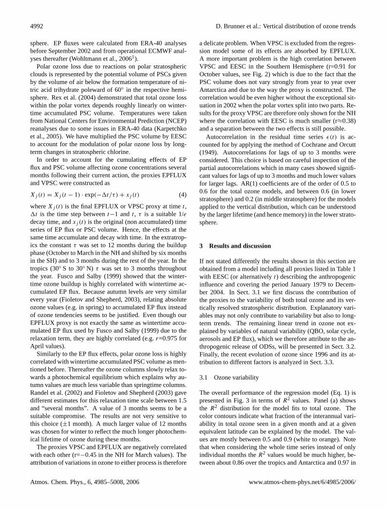
The overall performance of the regression model (Eq.1) ispresented in Fig.3 in terms ofR2 values. Panel (a) showsthe R2 distribution for the model fits to total ozone. Thecolor contours indicate what fraction of the interannual vari-ability in total ozone seen in a given month and at a givenequivalent latitude can be explained by the model. The val-ues are mostly between 0.5 and 0.9 (white to orange). Notethat when considering the whole time series instead of onlyindividual months theR2 values would be much higher, be-tween about 0.86 over the tropics and Antarctica and 0.97 in
Atmos. Chem. Phys., 6, 4985–5008, 2006 www.atmos-chem-phys.net/6/4985/2006/
D. Brunner et al.: Vertical distribution of ozone trends 4993
(a) (b)
Fig. 3. Quality of regression model fits in terms of explained varianceR2. (a) Regression to the time series of monthly mean total ozoneas a function of equivalent latitude and month.(b) Regression to the monthly mean ozone volume mixing ratios as a function of equivalentlatitude and pressure. See text for further details.
northern and southern mid-latitudes, because the variabilityis usually dominated by the seasonal cycle which can be wellreproduced by a model following Eq. (1). A narrow bandof high R2 values at the equator is flanked by low valuesat about 10◦ on either side of the equator, which is a clearfeature of the QBO (see next section). In the subtropics andmid-latitudes, the values are generally high except during au-tumm in the respective hemisphere. During these months, theinterannual variability is generally very low and may be dom-inated by noise. Poleward of 60◦ the lowR2 values extendfrom autumn into winter when only little or no light reachesthe polar regions. During this time period polar vortex aircan only be observed by TOMS when it is pushed equator-ward by dynamic perturbations. As the Antarctic vortex ismuch less perturbed there is only little TOMS data availablefor assimilation into CATO. Nevertheless, CATO appears tosee an increasing proportion of the vortex starting at the edgein June and propagating to the pole by September. FromSeptember to December a very high fraction of the interan-nual variability can be reproduced by the regression model.Interestingly, the model shows a poor performance on theequatorward side of the vortex between 54◦ and 60◦ S. Pos-sibly this is due to the very large ozone gradients betweenair inside and outside of the vortex. CATO separates theseairmasses based on their equivalent latitude which in turn isbased on potential vorticity fields which are clearly not per-fect. Figure3b shows the fraction of interannual variabilityexplained as a function of equivalent latitude and pressureaveraged over all months. Note again, thatR2 values wouldbe mostly above 0.9 when seasonal variability were included.Below 10 hPaR2 values are mostly in the range 0.35 to 0.7with largest values where the variability is dominated by theQBO (see next section) or by polar vortex processes. Above10 hPa the model performance is mostly poor as expecteddue to the limitations in the CATO reconstruction method atthese altitudes.
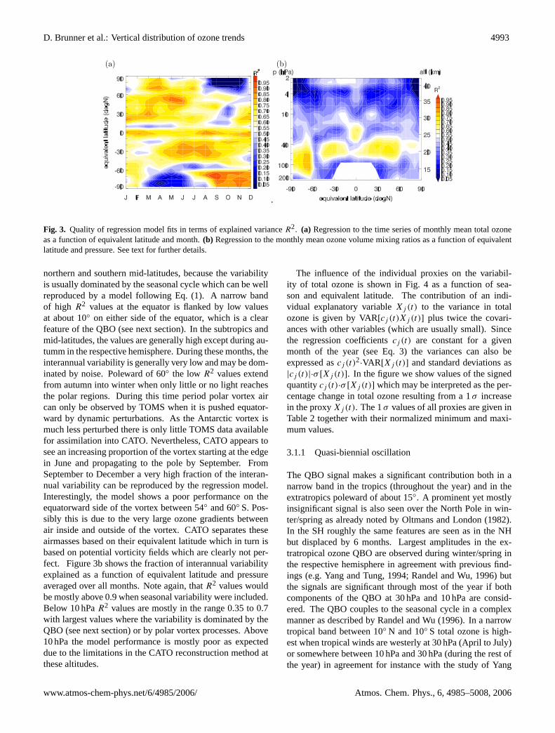
The influence of the individual proxies on the variabil-ity of total ozone is shown in Fig.4 as a function of sea-son and equivalent latitude. The contribution of an indi-vidual explanatory variableXj (t) to the variance in totalozone is given by VAR[cj (t)Xj (t)] plus twice the covari-ances with other variables (which are usually small). Sincethe regression coefficientscj (t) are constant for a givenmonth of the year (see Eq.3) the variances can also beexpressed ascj (t)
2·VAR[Xj (t)] and standard deviations as
|cj (t)|·σ [Xj (t)]. In the figure we show values of the signedquantitycj (t)·σ [Xj (t)] which may be interpreted as the per-centage change in total ozone resulting from a 1σ increasein the proxyXj (t). The 1σ values of all proxies are given inTable2 together with their normalized minimum and maxi-mum values.
3.1.1 Quasi-biennial oscillation
The QBO signal makes a significant contribution both in anarrow band in the tropics (throughout the year) and in theextratropics poleward of about 15◦. A prominent yet mostlyinsignificant signal is also seen over the North Pole in win-ter/spring as already noted byOltmans and London(1982).In the SH roughly the same features are seen as in the NHbut displaced by 6 months. Largest amplitudes in the ex-tratropical ozone QBO are observed during winter/spring inthe respective hemisphere in agreement with previous find-ings (e.g.Yang and Tung, 1994; Randel and Wu, 1996) butthe signals are significant through most of the year if bothcomponents of the QBO at 30 hPa and 10 hPa are consid-ered. The QBO couples to the seasonal cycle in a complexmanner as described byRandel and Wu(1996). In a narrowtropical band between 10◦ N and 10◦ S total ozone is high-est when tropical winds are westerly at 30 hPa (April to July)or somewhere between 10 hPa and 30 hPa (during the rest ofthe year) in agreement for instance with the study ofYang
www.atmos-chem-phys.net/6/4985/2006/ Atmos. Chem. Phys., 6, 4985–5008, 2006
4994 D. Brunner et al.: Vertical distribution of ozone trends
(a) QBO at 30 hPa (b) QBO at 10 hPa (c) Aerosols
(d) Solar cycle (e) EP flux (f) VPSC
Fig. 4. Contributions to variability in total ozone as a function of season and equivalent latitude. To show all figures in comparable units theregression coefficients were first multiplied by one standard deviation of each proxy time series and then divided by the 1979–2004 meanozone distribution. Values thus represent the percent change in total ozone for a 1σ increase in the corresponding proxy. Shading indicatesthat the values are statistically not significant at the 95% significance level. Contour line spacing is 1%.
and Tung(1995). In mid-latitudes, however, the phase lagbetween total ozone and the QBO is not constant as oftenassumed in other studies but changes continuously through-out the season. Between July and September, for instance,total ozone anomalies at northern mid-latitudes are in phasewith the QBO at 10 hPa but are in opposite phase betweenDecember and March.
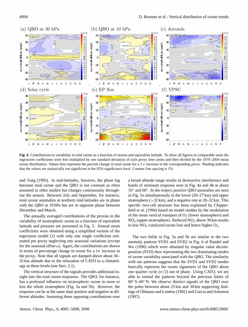
The annually averaged contributions of the proxies to thevariability of stratospheric ozone as a function of equivalentlatitude and pressure are presented in Fig.5. Annual meancoefficients were obtained using a simplified version of theregression model (1) with only one single coefficient esti-mated per proxy neglecting any seasonal variations (exceptfor the seasonal offseta). Again, the contributions are shownin terms of percentage change in ozone for a 1σ increase inthe proxy. Note that all signals are damped above about 30–35 km altitude due to the relaxation of CATO to a climatol-ogy at these levels (see Sect.2.1).
The vertical structure of the signals provides additional in-sight into the total ozone responses. The QBO, for instance,has a profound influence on stratospheric ozone in more orless the whole stratosphere (Fig.5a and5b). However, theresponse can be at the same time positive and negative at dif-ferent altitudes. Summing these opposing contributions over
a broad altitude range results in destructive interference andbands of mininum response seen in Fig.4a and4b at about10◦ and 60◦. In the tropics positive QBO anomalies are seenin Fig. 5a simultaneously in the lower (20–27 km) and upperstratosphere (>32 km), and a negative one at 28–32 km. Thisspecific two-cell structure has been explained byChipper-field et al.(1994) based on model studies by the modulationof the mean vertical transport of O3 (lower stratosphere) andNOy (upper stratosphere). Reduced NOy above 30 km resultsin less NOx-catalyzed ozone loss and hence higher O3.
The two fields in Fig.5a and5b are similar to the twoanomaly patterns SVD1 and SVD2 in Fig. 6 ofRandel andWu (1996) which were obtained by singular value decom-position (SVD) thus representing the two dominating modesof ozone variability associated with the QBO. The similaritywith our patterns suggests that the SVD1 and SVD2 modesbasically represent the ozone signatures of the QBO aboutone quarter cycle (π/2) out of phase. Using CATO, we areable to extend the patterns beyond the previous limits of60◦ S–60◦ N. We observe distinct signals of the QBO overthe poles between about 25 km and 30 km supporting find-ings ofOltmans and London(1982) andGarcia and Solomon(1987).
Atmos. Chem. Phys., 6, 4985–5008, 2006 www.atmos-chem-phys.net/6/4985/2006/
D. Brunner et al.: Vertical distribution of ozone trends 4995
(a) QBO at 30 hPa (b) QBO at 10 hPa (c) Aerosols
(d) Solar cycle (e) EP flux (f) VPSC
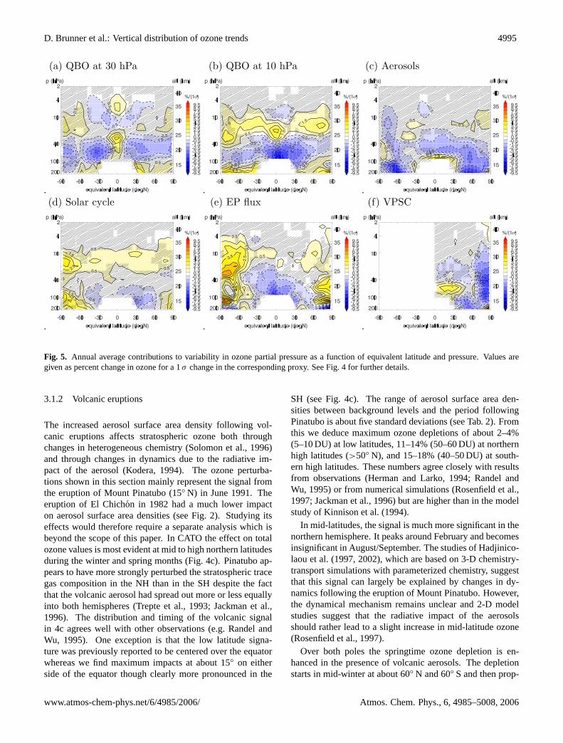
Fig. 5. Annual average contributions to variability in ozone partial pressure as a function of equivalent latitude and pressure. Values aregiven as percent change in ozone for a 1σ change in the corresponding proxy. See Fig.4 for further details.
3.1.2 Volcanic eruptions
The increased aerosol surface area density following vol-canic eruptions affects stratospheric ozone both throughchanges in heterogeneous chemistry (Solomon et al., 1996)and through changes in dynamics due to the radiative im-pact of the aerosol (Kodera, 1994). The ozone perturba-tions shown in this section mainly represent the signal fromthe eruption of Mount Pinatubo (15◦ N) in June 1991. Theeruption of El Chichon in 1982 had a much lower impacton aerosol surface area densities (see Fig.2). Studying itseffects would therefore require a separate analysis which isbeyond the scope of this paper. In CATO the effect on totalozone values is most evident at mid to high northern latitudesduring the winter and spring months (Fig.4c). Pinatubo ap-pears to have more strongly perturbed the stratospheric tracegas composition in the NH than in the SH despite the factthat the volcanic aerosol had spread out more or less equallyinto both hemispheres (Trepte et al., 1993; Jackman et al.,1996). The distribution and timing of the volcanic signalin 4c agrees well with other observations (e.g.Randel andWu, 1995). One exception is that the low latitude signa-ture was previously reported to be centered over the equatorwhereas we find maximum impacts at about 15◦ on eitherside of the equator though clearly more pronounced in the
SH (see Fig.4c). The range of aerosol surface area den-sities between background levels and the period followingPinatubo is about five standard deviations (see Tab.2). Fromthis we deduce maximum ozone depletions of about 2–4%(5–10 DU) at low latitudes, 11–14% (50–60 DU) at northernhigh latitudes (>50◦ N), and 15–18% (40–50 DU) at south-ern high latitudes. These numbers agree closely with resultsfrom observations (Herman and Larko, 1994; Randel andWu, 1995) or from numerical simulations (Rosenfield et al.,1997; Jackman et al., 1996) but are higher than in the modelstudy ofKinnison et al.(1994).
In mid-latitudes, the signal is much more significant in thenorthern hemisphere. It peaks around February and becomesinsignificant in August/September. The studies ofHadjinico-laou et al.(1997, 2002), which are based on 3-D chemistry-transport simulations with parameterized chemistry, suggestthat this signal can largely be explained by changes in dy-namics following the eruption of Mount Pinatubo. However,the dynamical mechanism remains unclear and 2-D modelstudies suggest that the radiative impact of the aerosolsshould rather lead to a slight increase in mid-latitude ozone(Rosenfield et al., 1997).
Over both poles the springtime ozone depletion is en-hanced in the presence of volcanic aerosols. The depletionstarts in mid-winter at about 60◦ N and 60◦ S and then prop-
www.atmos-chem-phys.net/6/4985/2006/ Atmos. Chem. Phys., 6, 4985–5008, 2006
4996 D. Brunner et al.: Vertical distribution of ozone trends
agates poleward. Over Antarctica the depletion reaches itsmaximum not before November and hence appears to be sig-nificantly delayed relative to the ozone depletion on PSCsexpected to peak in October. These results are in good cor-respondence with the model study ofRosenfield et al.(1997)who explained the delay over the south pole by the effectsof the aerosol on photolysis rates leading to more Cly beingstored as HOCl rather than Cl2 during polar night. HOCl isless readily photolyzed than Cl2 leading to a delayed buildupof ClOx.
The vertical distribution of the annual mean ozone re-sponse to volcanic eruptions shows negative values through-out the lower stratosphere maximizing at about 60◦ where itextends down to the tropopause level in both hemispheres(Fig. 5c). In the SH extratropics the signal mainly oc-curs below 100 hPa which may explain why it has beenmissed in previous analyses of satellite data. In the tropicsa significantly negative response is found above the tropi-cal tropopause up to about 28 km. In northern mid- to highlatitudes there is a change from negative to positive influ-ences at 25 km altitude. This agrees very well with ozoneanomalies measured from sondes at Boulder, USA (40◦ N)(Hofmann et al., 1994), which show a change to positive val-ues at 24 km. The model studies ofRosenfield et al.(1997),Solomon et al.(1996) and Zhao et al.(1997) suggest thatin the extratropics the main reason for this change in signis heterogeneous chemistry on the increased aerosol surface.Heterogeneous reactions reduce the concentration of NOxbut increase ClOx and HOx. Reduced NOx leads to moreozone above 25 km whereas below that level the increases inClOx and HOx outweigh the reductions in NOx leading to en-hanced ozone depletion. The good agreement of CATO withthese studies supports the notion ofSolomon et al.(1996)that heterogeneous chemistry played an important role inshaping the ozone response in northern mid-latitudes in addi-tion to the dynamical effects proposed byHadjinicolaou et al.(1997).
3.1.3 11-year solar cycle
The effect of the 11-year solar cycle on total ozone is shownin Fig. 4d. An accurate account for solar variability isessential since it may significantly affect ozone trend es-timates (World Meteorological Organization, 2003; Stein-brecht et al., 2004). However, there is presently little con-sensus on the exact structure of the solar cycle signal andsuch estimates generally suffer from the short data recordsand from the temporal alignment of the solar cycles with theeruptions of El Chichon and Pinatubo (Solomon et al., 1996;McCormack et al., 1997; Lee and Smith, 2003). Includingthe latest cycle (cycle 23) should allow us to better separatebetween the different effects as it was not synchronized witha major volcanic eruption (see Fig.2). A further complica-tion is that solar cycle effects at high latitudes are modulatedby the QBO (Labitzke and van Loon, 2000) or rather, that
the QBO itself is modulated by the solar cycle (Salby andCallaghan, 2000). More recent model and observation-basedstudies support the initial findings of (Salby and Callaghan,2000) that solar variability induces a decadal-scale modu-lation of the QBO period (McCormack, 2003; Salby andCallaghan, 2006). An example for the connection betweenQBO and solar effects is the observation that solar cycle vari-ations in total ozone are significantly larger during easterlyphases of the QBO than during westerly phases (Steinbrechtet al., 2003). A second problem affecting the separation be-tween QBO and solar effects is caused by the interactionbetween the annual cycle and the QBO which can inducea decadal scale oscillation (Salby et al., 1997). This oscil-lation happened to be 180◦ out of phase with the solar fluxvariation during cycles 21 and 22. Solar variability regres-sion analyzes based on this time period therefore seem to bestrongly affected by interferences with QBO as demonstratedby Lee and Smith(2003). As for the aerosols, the latest so-lar cycle was not synchronized with the QBO in the sameway the previous cycles allowing for a somewhat better sep-aration of the different effects. This may explain differencesbetween our results and earlier studies to some degree.
As shown in Fig.4d total ozone is generally elevated dur-ing periods of maximum solar activity (e.g.Brasseur, 1993;Hood, 1997; Steinbrecht et al., 2003). The low latitude signalappears to be strongest between January and July but sea-sonal differences are generally small. Similar to the abovestudies we find that the amplitude of the signal has a localminimum near the equator. The 2-D model study ofBrasseur(1993) reported a steady increase in the signal from the equa-tor towards the poles which contrasts with the pattern de-rived from CATO. Significant regression coefficients are infact only found between 10◦ and 35◦ in the NH and some-what closer to the equator in the SH. The signal is mostly in-significant in mid-latitudes and is again larger over the polesduring the respective spring season, in agreement with thestudy ofBrasseur(1993). The modification of polar strato-spheric temperatures and geopotential height by the 11-yearsolar cycle during the northern winter is well documented(Labitzke, 1987; van Loon and Labitzke, 1994) whereas theinfluence on the high latitude ozone distribution is much lesswell known due to a lack of observations. Our results indi-cate that total ozone over Antarctica is sensitive to solar cyclevariability in particular during late spring. Since the rangeof Mg II index values is about 3.5 standard deviations (Ta-ble2), total ozone is up to 10% higher over Antarctica duringsolar maximum than during solar minimum which contraststrongly with the value of less than 2% derived byBrasseur(1993). At low latitudes we find the changes to be below 3%.
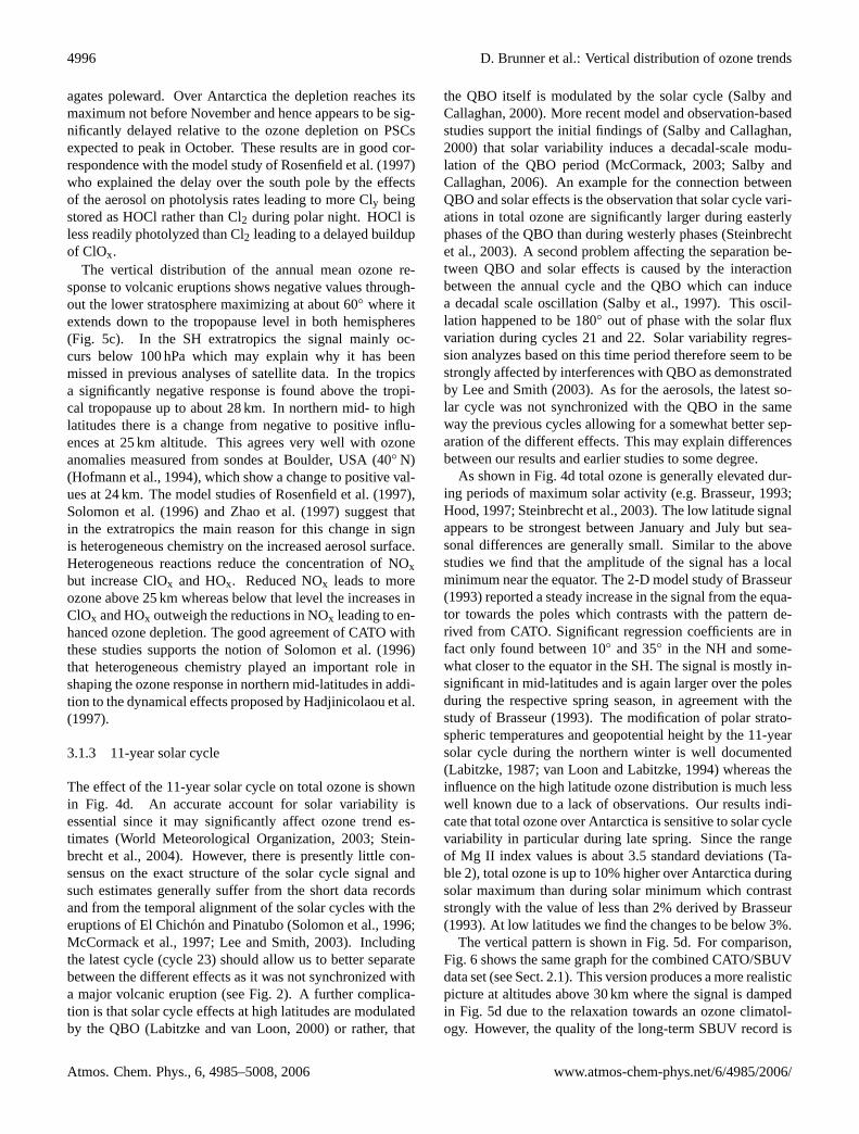
The vertical pattern is shown in Fig.5d. For comparison,Fig. 6 shows the same graph for the combined CATO/SBUVdata set (see Sect.2.1). This version produces a more realisticpicture at altitudes above 30 km where the signal is dampedin Fig. 5d due to the relaxation towards an ozone climatol-ogy. However, the quality of the long-term SBUV record is
Atmos. Chem. Phys., 6, 4985–5008, 2006 www.atmos-chem-phys.net/6/4985/2006/
D. Brunner et al.: Vertical distribution of ozone trends 4997
under debate because of intersatellite calibration issues (e.g.Steinbrecht et al., 2006). A second problem may be relatedto ERA-40 temperatures in the upper stratosphere which areknown to exhibit stepwise shifts due to the assimilation ofcertain satellite data (Uppala et al., 2005). The CATO/SBUVdata set is sensitive to errors in the ERA-40 temperatures be-cause the SBUV data were interpolated from pressure levelsonto the native potential temperature levels of CATO. Giventhese limitations and the general problems with disentanglingdifferent effects mentioned earlier, the results presented inthe following should be interpreted with care.
The main feature is a positive response maximizing atabout 10–20 hPa (27–32 km) with a relatively uniform dis-tribution extending from pole to pole. In the combinedCATO/SBUV data set the signal extends up to about 38 kmin mid-latitudes and up to the highest level (>40 km) overAntarctica. The solar cycle signal is located at lower alti-tudes than reported in the model studies ofBrasseur(1993),Langematz et al.(2005) and Lee and Smith(2003) (about32–38 km) but relatively close to the results ofEgorova et al.(2005) (30–35 km). It is also substantially lower than re-ported from previous observation studies. Results based onsatellite measurements suggested largest relative increasesfrom solar minimum to maximum occurring in mid-latitudesnear the stratopause between 40 and 50 km (McCormack andHood, 1996; Wang et al., 1996; Lee and Smith, 2003; Zere-fos et al., 2005). Unfortunately, this altitude range is notcovered in our analysis. These studies further reported ona significant negative anomaly in the tropical stratosphere at30–35 km (McCormack and Hood, 1996; Wang et al., 1996;Lee and Smith, 2003) or slightly higher (Zerefos et al., 2005)which is completely absent in our analysis. We do not findsuch a signal even if we exclude the latest solar cycle. Sucha negative signal contrasts with model results which tend toshow a generally positive response maximizing well below40 km with either a monopolar structure centered over thetropics (Lee and Smith, 2003), a relatively uniform signalbetween±60◦ (Brasseur, 1993; Egorova et al., 2004, 2005),or showing almost no change in the stratosphere (Huangand Brasseur, 1993). A weak negative signal in the tropi-cal lower stratosphere could only be reproduced byLange-matz et al.(2005) which was the first study to include anidealized source of NOx from high-energy electrons maxi-mizing during solar minimum. A similar dipole pattern as inthe observations could also be reproduced byLee and Smith(2003). However, they demonstrated that this is not due tosolar cycle variation but rather to the interference with QBOand volcanic eruptions in the statistical analysis.
As in total ozone the largest effects are seen over Antarc-tica with annually averaged ozone being enhanced by about7% during solar maximum relative to solar minimum above30 hPa as well as below 80 hPa. Over the Arctic the signalis generally much weaker and it is only mildly significant atthe upper levels. These observations provide some supportfor the 3-D numerical simulations ofLangematz et al.(2005)
Fig. 6. 11-year solar cycle signal in CATO version with SBUVVersion 8 data assimilated in upper stratosphere.
who found the largest ozone changes at polar latitudes.
3.1.4 Brewer-Dobson circulation
The Brewer-Dobson circulation has a profound impact on to-tal ozone concentrations at high northern latitudes betweenDecember and June (Fig.4e). It explains a dominant fractionof the generally large variability over this region. BetweenDecember and February the influence extends down to 40◦ N.Note that the ozone signal shown refers to one standard devi-ation of the EPFLUX proxy values of the respective month.January values, for instance, refer to one standard deviationof all January EPFLUX values. It is thus a measure of in-terannual variability rather than of the seasonal amplitude ofvariation which would be much larger. An intensified circu-lation is associated with a weak polar vortex and correspond-ingly high total ozone values over the poles and reduced val-ues at low latitudes (Fusco and Salby, 1999). Between 30◦
and 50◦ N the effect of EP flux variations is minimal. Thepattern is similar in the SH but shifted by six months. EPflux is strongest between October and February in the NHand drops to very low values between May and July. Theintegrated amount of EP flux entering the stratosphere overthe winter determines the buildup of ozone from autumn untilspring. Thereafter ozone concentrations relax towards photo-chemical equilibrium on a timescale of a few months (Randelet al., 2002; Fioletov and Shepherd, 2003). Total ozone there-fore remains correlated to the spring time values and henceto wintertime accumulated EP flux throughout the summer(Fioletov and Shepherd, 2003). This is also seen in Fig.4ewhere total ozone anomalies remain significantly influencedby EP flux until the following autumn.
www.atmos-chem-phys.net/6/4985/2006/ Atmos. Chem. Phys., 6, 4985–5008, 2006
4998 D. Brunner et al.: Vertical distribution of ozone trends
December January February
March May July
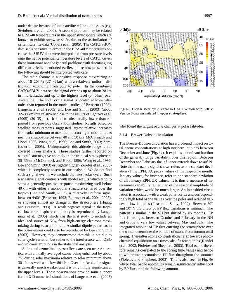
Fig. 7. Sequence of the influence of northern hemisphere EP flux variations on the global stratospheric ozone distribution in selected months.Values are given as percentage change in ozone for a 1σ change in the EPFLUX proxy in the given month.
In the SH the situation is somewhat more complicated.The EP flux is generally weaker due to lower wave activityand has a less pronounced annual cycle. Similar to the NHa positive anomaly appears in mid-latitudes in autumn andlasts until the following spring or actually somewhat longerin the SH. Yet, there is a distinct difference between the twohemispheres at polar latitudes. The signal appears much laterin the SH and also the peak influence is delayed by roughlytwo months. The absence of a strong signal between Apriland September is likely a consequence of the Antarctic vor-tex being much more isolated than the Arctic one as alreadynoted byDobson(1968). The Antarctic vortex is thereforeless disturbed by wave activity (and hence variations in EPflux) which may for instance lead to sudden stratosphericwarmings in the NH but not in the SH.
The vertical distribution of the annual mean influence ofEP flux variations is shown in Fig.5e. Elevated ozone ismainly found poleward of 60◦ in the lower stratosphere anddown to about 40◦ above 25 km in both hemispheres. In theSH the positive anomaly in the lower stratosphere extends tolower latitudes which explains the more prominent anomalyseen in the total columns (Fig.4e). The enhanced transportto high latitudes is associated with a decrease in ozone inthe tropical lower stratosphere. This is clearly visible up toabout 25 km in the NH and somewhat higher up in the SH.Note that in each hemisphere we only accounted for the EPflux of the respective hemisphere. The influence of the NH
extratropical pump on the SH and vice versa is excluded inthis view.
Figure 7 therefore shows a sequence of the influence ofNH EP flux only on the global ozone distribution for selectedmonths. As expected, the influence builds up in the NHfrom December to March/April and weakens thereafter. Thelargest buildup occurs north of 60◦ N below 23 km. Above25 km a positive anomaly is located at about 50◦ N in De-cember which appears to slowly progress northwards untilMarch. The region of reduced ozone in the tropical lowerstratosphere (<24 km) extends well into the SH as reportedalso by Fusco and Salby(1999) based on MLS measure-ments. Negative ozone responses are not only seen near theequator but at least up to 50◦ S in the lower stratosphere.
At higher levels above 22–25 km the response to increasedEP flux is positive in both hemispheres. The positive signal inthe SH is strongest between January and March and appearsto have a local maximum around 50◦ S. This anomaly maybe related to the strongly enhanced upward transport in theSH upper stratosphere (maximum at about 20◦ S) reportedby (Solomon et al., 1986) which produces a strong increasein CH4 and N2O from November to February as observedfrom satellites. Using a prognostic model,Solomon et al.(1986) demonstrated that this transport is not induced locallybut rather by forcing from the northern hemisphere. Simi-larly, Salby and Callaghan(2004) analyzed tendencies (e.g.from November to March) of ozone and meteorological pa-
Atmos. Chem. Phys., 6, 4985–5008, 2006 www.atmos-chem-phys.net/6/4985/2006/
D. Brunner et al.: Vertical distribution of ozone trends 4999
rameters and found that amplified wave forcing in the win-ter hemisphere leads to anomalous upwelling in the summerhemisphere, with largest changes over the polar cap. Ac-cording to their analysis, the ozone response in the summer-time polar stratosphere is thus in phase with the responsein the tropics. This seems to be confirmed by Fig.7 whereJanuary and February anomalies are significantly negative inthe Antarctic lower stratosphere, in phase with the negativetropical anomalies. In the NH, the polar anomaly signifi-cantly weakens between March and July which is a result ofrapid mixing throughout the extratropics once the polar vor-tex breaks down (Fioletov and Shepherd, 2005). As a resultthe ozone anomalies remain positive in the lower stratosphere(>100 hPa) in mid-latitudes between May and July. Above20 km altitude a positive anomaly remains until at least Julywhich is in good agreement with results from a Lagrangianmodel study byKonopka et al.(2003) which demonstratesthat vortex remnants at this level are “frozen in” in the sum-mer circulation without much mixing.
3.1.5 Ozone depletion on PSCs
For reasons described in Sect.2.2 results for the variableVPSC are only shown for the NH. As expected, the influ-ence on total ozone is strongest between February and Aprilnorth of 70◦ N (Fig. 4f). Interestingly, the anomaly spreadsto low latitudes, i.e. down to at least 30◦ N, between Apriland July suggesting a significant impact of polar ozone de-pletion on mid-latitude ozone during summer. Notably thiseffect can not be reproduced by EPFLUX even if VPSC isexcluded from the regression model. Given the fact that therange between minimum and maximum PSC volume is about4 standard deviations (see Tab.2) we may estimate that mid-latitude ozone is up to 4% lower in a summer following acold Arctic winter than following a warm winter due to theeffect of polar ozone depletion alone. Using a 3-D chemistry-transport-model,Chipperfield(1999) calculated reductionsof 2–3% at 50◦ N due to the effects of chlorine activationon cold liquid aerosols, nitric acid trihydrate and ice parti-cles. Compared to our results these values are too low inparticular given the fact that they do not only include po-lar but also mid-latitude heterogeneous ozone losses. Sim-ilar problems have been reported for other numerical sim-ulations (World Meteorological Organization, 2003) but re-cent model updates have strongly improved the agreementwith observed Arctic ozone depletion (Chipperfield et al.,2005). Knudsen and Groß(2000) used reverse domain fill-ing trajectories to calculate the dilution of mid-latitude airby ozone depleted air from the vortex. They found reduc-tions in 30◦−60◦ N mean total ozone due to dilution of theorder of 3% in spring 1995 and 1997, respectively, followingtwo exceptionally cold Arctic winters. The dilution effect ex-tends down to about 30◦ N within the first two months afterbreakup of the vortex. These results agree well with our esti-mate of a maximum effect of 4% and the seasonal evolution
shown in Fig.4f.Unlike the pattern for total ozone the vertical distribution
is quite noisy as seen in Fig.5f. The problems of the regres-sion analysis to distinguish between effects of VPSC and ef-fects of EPFLUX is quite obvious when comparing panels eand f. At high northern latitudes at 17 km for instance, the EPflux signal shows a pronounced minimum. This minimumis compensated by VPSC which shows a distinct negativemaximum at the same place. VPSC contributions are largestnorth of about 65◦ N as expected, but contributions are alsoseen in the lower stratosphere (13–17 km) in mid-latitudes.As suggested by Fig.4f, the latter is probably due to south-ward transport of polar air depleted in ozone between Apriland July following the break-up of the polar vortex. The lowlatitude signals south of 40◦ N are probably due to the im-perfect separation between EP flux and VPSC effects. In asimulation excluding VPSC the EP flux anomalies tend tobecome more pronounced at these points.
3.2 Ozone trends
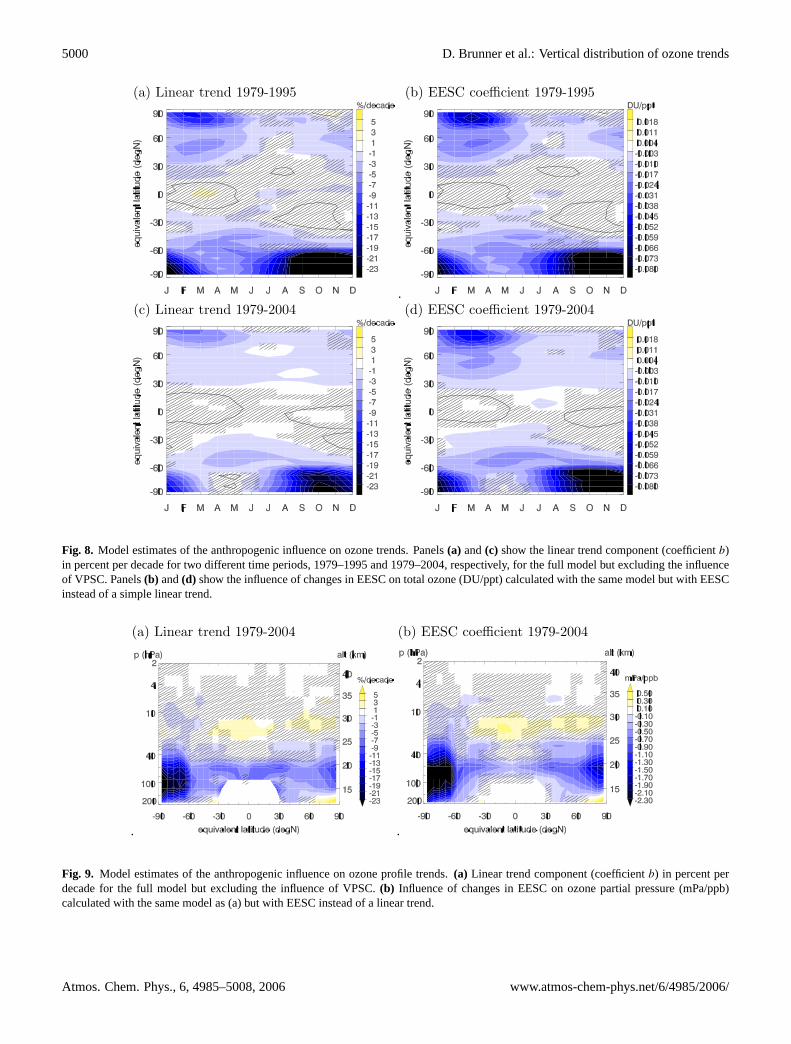
Figure 8 compares residual linear trends (coefficientb inEq. 1 and 2) in total ozone estimated for the period 1979to 1995 (upper panels) and for 1979 to 2004 (lower panels).The term “residual” in this context means that the influenceof natural variability, i.e. of volcanic aerosols, solar cycle,EP flux and QBO, on the trend is removed. Results are onlyshown for the model excluding VPSC because this proxy alsocontains an anthropogenic component (due to multiplicationby EESC) and because of its collinearity with EESC in theSH. The figures can thus be interpreted as representing theoverall trend due to man-made increases in EESC which in-fluences both polar processes as well as ozone depletion atnon-polar latitudes. It should be cautioned that over Antarc-tica a linear model is of limited value because after 1987ozone depletion continued at a smaller rate than before rel-ative to the increase in EESC due to saturation of the ozonedepletion in the vortex interior (Jiang et al., 1996).
The two left-hand panels are linear trends (in %/decaderelative to the period mean ozone) whereas the right-handpanels show the influence of EESC (in DU/ppt) directly.Because EESC increased almost linearly between 1979 and1995 (see Fig.2) panels (a) and (b) look very similar. For theperiod 1979 to 2004, however, the two panels (c) and (d) aredistinctly different. The linear trend is significantly smallerthan for 1979 to 1995, in particular for mid- to high lati-tudes in winter and spring in the respective hemisphere. Thissuggests that even after removing the influences of naturalvariability the ozone trend was substantially lower (i.e. lessnegative or even positive) after 1995 than before. The proxyEESC represents the anthropogenic influence more directly.Because EESC reached a maximum in 1997 and started de-creasing thereafter it seems to better represent the evolutionof ozone than a simple linear trend. The EESC coefficientsare in fact similar for both periods (compare panels b and d)
www.atmos-chem-phys.net/6/4985/2006/ Atmos. Chem. Phys., 6, 4985–5008, 2006
5000 D. Brunner et al.: Vertical distribution of ozone trends
(a) Linear trend 1979-1995 (b) EESC coefficient 1979-1995
(c) Linear trend 1979-2004 (d) EESC coefficient 1979-2004
Fig. 8. Model estimates of the anthropogenic influence on ozone trends. Panels(a) and(c) show the linear trend component (coefficientb)in percent per decade for two different time periods, 1979–1995 and 1979–2004, respectively, for the full model but excluding the influenceof VPSC. Panels(b) and(d) show the influence of changes in EESC on total ozone (DU/ppt) calculated with the same model but with EESCinstead of a simple linear trend.
(a) Linear trend 1979-2004 (b) EESC coefficient 1979-2004
Fig. 9. Model estimates of the anthropogenic influence on ozone profile trends.(a) Linear trend component (coefficientb) in percent perdecade for the full model but excluding the influence of VPSC.(b) Influence of changes in EESC on ozone partial pressure (mPa/ppb)calculated with the same model as (a) but with EESC instead of a linear trend.
Atmos. Chem. Phys., 6, 4985–5008, 2006 www.atmos-chem-phys.net/6/4985/2006/
D. Brunner et al.: Vertical distribution of ozone trends 5001
confirming that ozone and EESC evolved in a similar wayafter 1995. This point is analyzed in more detail in Sect.3.3.
In the NH the largest negative trends are seen in Febru-ary and March at high equivalent latitudes, i.e. within thepolar vortex, with values of up to−13%/decade for 1979–1995 and up to−9%/decade for 1979–2004. Notably thereis a second maximum at mid-latitudes around March whichseems to be detached from the polar maximum and whichoccurs too early to be explained by dilution with vortex air.This is likely an indication of mid-latitude ozone depletionwhich is thought to be controlled by heterogenous chem-istry leading to enhanced chlorine activation (Solomon et al.,1996). Since this process is closely related to the reductionof NOx by hydrolysis of N2O5 on aerosols it is conceivablethat its effect is strongest during winter when N2O5 hydrol-ysis is largest. Trends in mid-latitudes are largest in Marchand are of the order of−5%/decade for 1979–1995 but only−2%/decade for 1979–2004. EESC decreased by 195 pptfrom its maximum in 1997 to the end of 2004. Given regres-sion coefficients of about 0.018 DU/ppt in mid-latitudes and0.055 DU/ppt at polar latitudes this corresponds to an ozoneincrease since 1997 of up to 3.5 DU in mid-latitudes and upto 11 DU over the Arctic, respectively, due to the effects ofthe Montreal Protocol. A much larger recovery of the orderof 20 DU is expected for Antarctic springtime ozone. How-ever, EESC as used here is not representative for the Arcticand Antarctic stratosphere. Because the air is much older inthe polar stratosphere the peak in EESC will likely be de-layed here by some 2 to 3 years as compared to mid-latitudes(Newman et al., 2006). Hence, a significant increase in ozoneowing to the reduction in EESC cannot yet be expected by theend of 2004.
SH mid-latitude trends are similar to those in the NH withvalues of−3% to −5%/decade for 1979–1995 and about−2% to −3%/decade for 1979–2004. Negative trends tendto be largest in April/May which appears to be too late tobe explained by dilution with vortex air depleted in ozone.The seasonal variation of the trend is generally much smallerthan in the NH. Near the equator long-term trends are closeto zero and mostly insignificant.
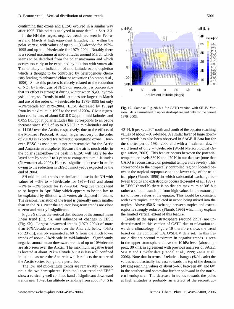
Figure9 shows the vertical distribution of the annual meanlinear trend (Fig.9a) and influence of changes in EESC(Fig. 9b). Largest downward trends (1979–2004) of morethan 20%/decade are seen over the Antarctic below 40 hPa(or 23 km), sharply separated at 60◦ S from the much lowertrends of about -5%/decade in mid-latitudes. Significantlynegative annual mean downward trends of up to 10%/decadeare also seen over the Arctic. The maximum negative trendis located at about 19 km altitude but it is less well confinedin latitude as over the Antarctic which reflects the nature ofthe Arctic vortex being more perturbed.
The low and mid-latitude trends are remarkably symmet-ric in the two hemispheres. Both the linear trend and EESCshow a vertically well confined band of significant downwardtrends near 18–20 km altitude extending from about 40◦ S to
Fig. 10. Same as Fig.9b but for CATO version with SBUV Ver-sion 8 data assimilated in upper stratosphere and only for the period1979–2003.
40◦ N. It peaks at 30◦ north and south of the equator reachingvalues of about−8%/decade. A similar layer of large down-ward trends has also been observed in SAGE-II data but forthe shorter period 1984–2000 and with a maximum down-ward trend of only−4%/decade (World Meteorological Or-ganization, 2003). This feature occurs between the potentialtemperature levels 380 K and 470 K in our data set (note thatCATO is reconstructed on potential temperature levels). Thiscorresponds to the “tropically controlled region” located be-tween the tropical tropopause and the lower edge of the trop-ical pipe (Plumb, 1996) in which substantial exchange be-tween tropics and extratropics occurs (Rosenlof et al., 1997).In EESC (panel b) there is no distinct maximum at 30◦ butrather a smooth transition from high values in the extratrop-ics to lowest values at the equator. This would be consistentwith extratropical air depleted in ozone being mixed into thetropics. Above 450 K exchange between tropics and extrat-ropics is strongly reduced (Plumb, 1996) which may explainthe limited vertical extent of this feature.
Trends in the upper stratosphere (around 2 hPa) are un-derestimated in this version of CATO due to relaxation to-wards a climatology. Figure10 therefore shows the trendbased on the combined CATO/SBUV data set. In this fig-ure a distinct second maximum in negative trends is seenin the upper stratosphere above the 10 hPa level (above ap-prox. 30 km), in agreement with previous analyzes of SAGE,SBUV and Umkehr data (Randel et al., 1999; Zanis et al.,2006). Note that in terms of relative changes (%/decade) thevalues would actually increase towards the top of the domain(40 km) reaching values of about 5–6% between 40◦ and 60◦
in the southern and somewhat further poleward in the north-ern hemisphere. The decrease in trends towards the polesat high altitudes is probably an artefact of the reconstruc-
www.atmos-chem-phys.net/6/4985/2006/ Atmos. Chem. Phys., 6, 4985–5008, 2006
5002 D. Brunner et al.: Vertical distribution of ozone trends
30 D. Brunner et al.: Vertical distribution of ozone trends
(a) EESC + QBO + SF (b) EESC + QBO + SF + AERO
(c) EESC + QBO + SF + AERO + EPFLUX (d) Linear trend + QBO + SF + AERO + EPFLUX
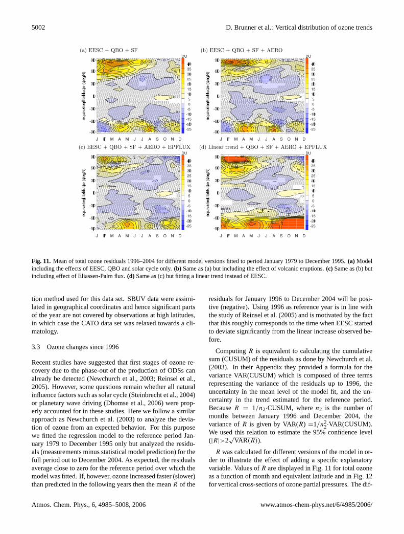
Fig. 11. Mean of total ozone residuals 1996–2004 for different model versions fitted to period January 1979 to December 1995.(a) Modelincluding the effects of EESC, QBO and solar cycle only.(b) Same as (a) but including the effect of volcanic eruptions.(c) Same as (b) butincluding effect of Eliassen-Palm flux.(d) Same as (c) but fitting a linear trend instead of EESC.
Atmos. Chem. Phys., 0000, 0001–32, 2006 www.atmos-chem-phys.org/acp/0000/0001/
Fig. 11. Mean of total ozone residuals 1996–2004 for different model versions fitted to period January 1979 to December 1995.(a) Modelincluding the effects of EESC, QBO and solar cycle only.(b) Same as (a) but including the effect of volcanic eruptions.(c) Same as (b) butincluding effect of Eliassen-Palm flux.(d) Same as (c) but fitting a linear trend instead of EESC.
tion method used for this data set. SBUV data were assimi-lated in geographical coordinates and hence significant partsof the year are not covered by observations at high latitudes,in which case the CATO data set was relaxed towards a cli-matology.
3.3 Ozone changes since 1996
Recent studies have suggested that first stages of ozone re-covery due to the phase-out of the production of ODSs canalready be detected (Newchurch et al., 2003; Reinsel et al.,2005). However, some questions remain whether all naturalinfluence factors such as solar cycle (Steinbrecht et al., 2004)or planetary wave driving (Dhomse et al., 2006) were prop-erly accounted for in these studies. Here we follow a similarapproach asNewchurch et al.(2003) to analyze the devia-tion of ozone from an expected behavior. For this purposewe fitted the regression model to the reference period Jan-uary 1979 to December 1995 only but analyzed the residu-als (measurements minus statistical model prediction) for thefull period out to December 2004. As expected, the residualsaverage close to zero for the reference period over which themodel was fitted. If, however, ozone increased faster (slower)than predicted in the following years then the meanR of the
residuals for January 1996 to December 2004 will be posi-tive (negative). Using 1996 as reference year is in line withthe study ofReinsel et al.(2005) and is motivated by the factthat this roughly corresponds to the time when EESC startedto deviate significantly from the linear increase observed be-fore.
ComputingR is equivalent to calculating the cumulativesum (CUSUM) of the residuals as done byNewchurch et al.(2003). In their Appendix they provided a formula for thevariance VAR(CUSUM) which is composed of three termsrepresenting the variance of the residuals up to 1996, theuncertainty in the mean level of the model fit, and the un-certainty in the trend estimated for the reference period.BecauseR = 1/n2·CUSUM, wheren2 is the number ofmonths between January 1996 and December 2004, thevariance ofR is given by VAR(R) =1/n2
2·VAR(CUSUM).We used this relation to estimate the 95% confidence level(|R|>2
√VAR(R)).
R was calculated for different versions of the model in or-der to illustrate the effect of adding a specific explanatoryvariable. Values ofR are displayed in Fig.11 for total ozoneas a function of month and equivalent latitude and in Fig.12for vertical cross-sections of ozone partial pressures. The dif-
Atmos. Chem. Phys., 6, 4985–5008, 2006 www.atmos-chem-phys.net/6/4985/2006/
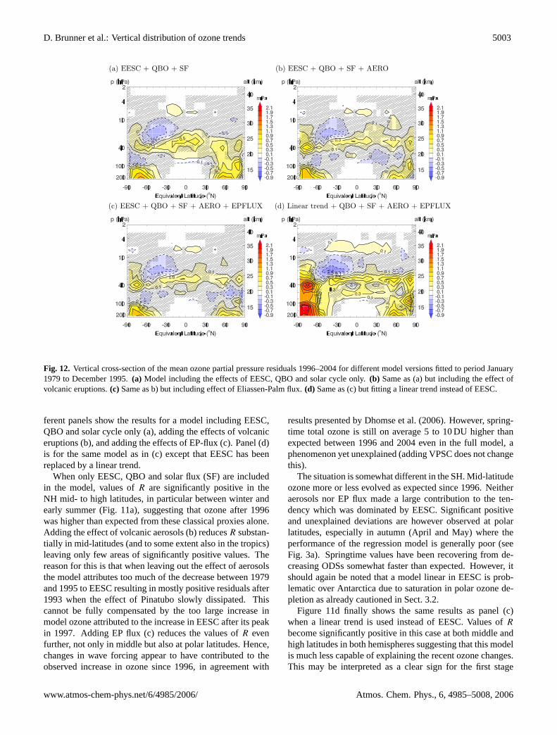
D. Brunner et al.: Vertical distribution of ozone trends 5003
D. Brunner et al.: Vertical distribution of ozone trends 31
(a) EESC + QBO + SF (b) EESC + QBO + SF + AERO
(c) EESC + QBO + SF + AERO + EPFLUX (d) Linear trend + QBO + SF + AERO + EPFLUX
Fig. 12. Vertical cross-section of the mean ozone partial pressure residuals 1996–2004 for different model versions fitted to period January1979 to December 1995.(a) Model including the effects of EESC, QBO and solar cycle only.(b) Same as (a) but including the effect ofvolcanic eruptions.(c) Same as b) but including effect of Eliassen-Palm flux.(d) Same as (c) but fitting a linear trend instead of EESC.
www.atmos-chem-phys.org/acp/0000/0001/ Atmos. Chem. Phys., 0000, 0001–32, 2006
Fig. 12. Vertical cross-section of the mean ozone partial pressure residuals 1996–2004 for different model versions fitted to period January1979 to December 1995.(a) Model including the effects of EESC, QBO and solar cycle only.(b) Same as (a) but including the effect ofvolcanic eruptions.(c) Same as b) but including effect of Eliassen-Palm flux.(d) Same as (c) but fitting a linear trend instead of EESC.
ferent panels show the results for a model including EESC,QBO and solar cycle only (a), adding the effects of volcaniceruptions (b), and adding the effects of EP-flux (c). Panel (d)is for the same model as in (c) except that EESC has beenreplaced by a linear trend.
When only EESC, QBO and solar flux (SF) are includedin the model, values ofR are significantly positive in theNH mid- to high latitudes, in particular between winter andearly summer (Fig.11a), suggesting that ozone after 1996was higher than expected from these classical proxies alone.Adding the effect of volcanic aerosols (b) reducesR substan-tially in mid-latitudes (and to some extent also in the tropics)leaving only few areas of significantly positive values. Thereason for this is that when leaving out the effect of aerosolsthe model attributes too much of the decrease between 1979and 1995 to EESC resulting in mostly positive residuals after1993 when the effect of Pinatubo slowly dissipated. Thiscannot be fully compensated by the too large increase inmodel ozone attributed to the increase in EESC after its peakin 1997. Adding EP flux (c) reduces the values ofR evenfurther, not only in middle but also at polar latitudes. Hence,changes in wave forcing appear to have contributed to theobserved increase in ozone since 1996, in agreement with
results presented byDhomse et al.(2006). However, spring-time total ozone is still on average 5 to 10 DU higher thanexpected between 1996 and 2004 even in the full model, aphenomenon yet unexplained (adding VPSC does not changethis).
The situation is somewhat different in the SH. Mid-latitudeozone more or less evolved as expected since 1996. Neitheraerosols nor EP flux made a large contribution to the ten-dency which was dominated by EESC. Significant positiveand unexplained deviations are however observed at polarlatitudes, especially in autumn (April and May) where theperformance of the regression model is generally poor (seeFig. 3a). Springtime values have been recovering from de-creasing ODSs somewhat faster than expected. However, itshould again be noted that a model linear in EESC is prob-lematic over Antarctica due to saturation in polar ozone de-pletion as already cautioned in Sect.3.2.
Figure 11d finally shows the same results as panel (c)when a linear trend is used instead of EESC. Values ofR
become significantly positive in this case at both middle andhigh latitudes in both hemispheres suggesting that this modelis much less capable of explaining the recent ozone changes.This may be interpreted as a clear sign for the first stage
www.atmos-chem-phys.net/6/4985/2006/ Atmos. Chem. Phys., 6, 4985–5008, 2006
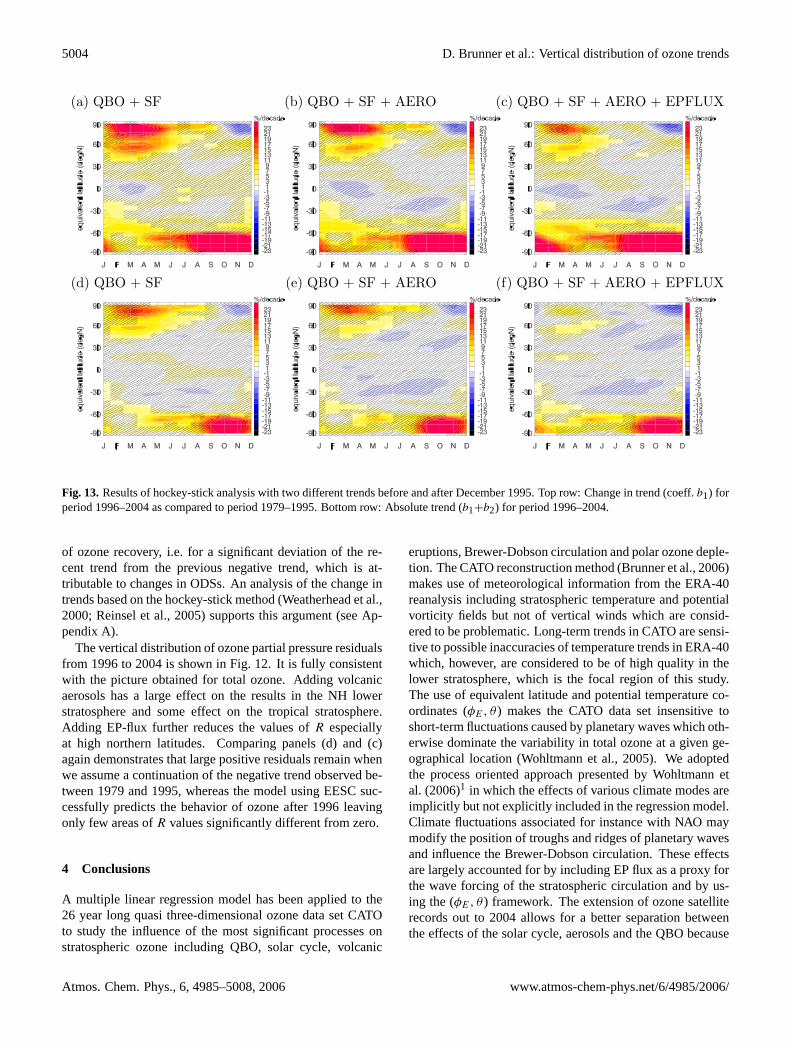
5004 D. Brunner et al.: Vertical distribution of ozone trends
32 D. Brunner et al.: Vertical distribution of ozone trends
(a) QBO + SF (b) QBO + SF + AERO (c) QBO + SF + AERO + EPFLUX
(d) QBO + SF (e) QBO + SF + AERO (f) QBO + SF + AERO + EPFLUX
Fig. 13. Results of hockey-stick analysis with two different trends before and after December 1995. Top row: Change in trend (coeff.b1) forperiod 1996–2004 as compared to period 1979 - 1995. Bottom row: Absolute trend (b1+b2) for period 1996–2004.
Atmos. Chem. Phys., 0000, 0001–32, 2006 www.atmos-chem-phys.org/acp/0000/0001/
Fig. 13.Results of hockey-stick analysis with two different trends before and after December 1995. Top row: Change in trend (coeff.b1) forperiod 1996–2004 as compared to period 1979–1995. Bottom row: Absolute trend (b1+b2) for period 1996–2004.
of ozone recovery, i.e. for a significant deviation of the re-cent trend from the previous negative trend, which is at-tributable to changes in ODSs. An analysis of the change intrends based on the hockey-stick method (Weatherhead et al.,2000; Reinsel et al., 2005) supports this argument (see Ap-pendix A).
The vertical distribution of ozone partial pressure residualsfrom 1996 to 2004 is shown in Fig.12. It is fully consistentwith the picture obtained for total ozone. Adding volcanicaerosols has a large effect on the results in the NH lowerstratosphere and some effect on the tropical stratosphere.Adding EP-flux further reduces the values ofR especiallyat high northern latitudes. Comparing panels (d) and (c)again demonstrates that large positive residuals remain whenwe assume a continuation of the negative trend observed be-tween 1979 and 1995, whereas the model using EESC suc-cessfully predicts the behavior of ozone after 1996 leavingonly few areas ofR values significantly different from zero.
4 Conclusions
A multiple linear regression model has been applied to the26 year long quasi three-dimensional ozone data set CATOto study the influence of the most significant processes onstratospheric ozone including QBO, solar cycle, volcanic
eruptions, Brewer-Dobson circulation and polar ozone deple-tion. The CATO reconstruction method (Brunner et al., 2006)makes use of meteorological information from the ERA-40reanalysis including stratospheric temperature and potentialvorticity fields but not of vertical winds which are consid-ered to be problematic. Long-term trends in CATO are sensi-tive to possible inaccuracies of temperature trends in ERA-40which, however, are considered to be of high quality in thelower stratosphere, which is the focal region of this study.The use of equivalent latitude and potential temperature co-ordinates (φE, θ ) makes the CATO data set insensitive toshort-term fluctuations caused by planetary waves which oth-erwise dominate the variability in total ozone at a given ge-ographical location (Wohltmann et al., 2005). We adoptedthe process oriented approach presented by Wohltmann etal. (2006)1 in which the effects of various climate modes areimplicitly but not explicitly included in the regression model.Climate fluctuations associated for instance with NAO maymodify the position of troughs and ridges of planetary wavesand influence the Brewer-Dobson circulation. These effectsare largely accounted for by including EP flux as a proxy forthe wave forcing of the stratospheric circulation and by us-ing the (φE, θ ) framework. The extension of ozone satelliterecords out to 2004 allows for a better separation betweenthe effects of the solar cycle, aerosols and the QBO because
Atmos. Chem. Phys., 6, 4985–5008, 2006 www.atmos-chem-phys.net/6/4985/2006/
D. Brunner et al.: Vertical distribution of ozone trends 5005
the latest solar cycle did not occur synchronously with a ma-jor volcanic disturbance and the QBO had a different phaserelation than during the previous two cycles.
The QBO was found to have a large influence on ozonevariability throughout the stratosphere. Volcanic eruptions(mainly Pinatubo) resulted in negative ozone anomalies inthe extratropical lower stratosphere below 25 km and weaklypositive anomalies above. In the tropics the region of de-pleted ozone reaches somewhat higher up. The largest ef-fects in terms of percentage ozone changes were found be-low 16 km around 60◦ in both hemispheres. Above that levelthe effects are much more pronounced in the NH. The solarcycle has a relatively minor positive effect on stratosphericozone maximizing at about 20◦ on both sides of the equatoras well as over the poles. Our analysis, which is limited to al-titudes below 40 km, indicates a maximum effect between 28and 32 km in the tropics and between about 25 and 38 km inthe extratropics, which is lower than suggested by previousstudies. Furthermore, we find no negative signal in the tropi-cal lower stratosphere which probably was an artefact of thestatistical analysis in previous studies (Lee and Smith, 2003).EP flux has a profound influence on the interannual variabil-ity of ozone. Enhanced wave forcing results in large pos-itive anomalies poleward of 60◦ and negative anomalies inthe tropical and subtropical lower stratosphere. Polar strato-spheric ozone depletion has only been analyzed for the north-ern hemisphere, where an up to 4% reduction in summer-time mid-latitude total ozone was found following cold Arc-tic winters, most likely as a result of dilution with air fromthe vortex.
Long-term trends are much less negative for the period1979 to 2004 compared to 1979 to 1995 suggesting a lev-elling off during the recent years. Fitting the model to theperiod 1979 to 1995 but analyzing the residuals out to 2004shows that the ozone changes since 1996 can not be under-stood by assuming a persistent negative trend. A model us-ing EESC instead of a linear trend, on the other hand, quitesuccessfully explains the recent changes, at least when theeffects of aerosols and of EP flux changes are accountedfor. Even then, lower stratospheric ozone increases since1996 were somewhat larger in the northern hemisphere dur-ing spring and over Antarctica during most of the year thanwe are presently able to explain.
Appendix A
Hockey-stick analysis of trend since 1996
As suggested byReinsel et al.(2005) a hockey-stick ap-proach can be used to detect a change in trend after a givenreference date relative to the trend before. In this case twoseparate linear trend componentsb1(t) andb2(t) are included
in the regression model which then reads as
Y (t) = a + b1 · t + b2 · t96 +
N∑j=1
cj · Xj (t) + ε(t) (A1)
wheret96 is a linear ramp function which is equal to zero be-fore December 1995 and after that is equal to the number ofmonths since December 1995. The coefficientb1 thus rep-resents the trend between 1979 and 1995,b2 is the changefrom this trend, andb1 + b2 is the absolute trend for the pe-riod 1996 to 2004. A positive value ofb2 thus only indicatesa positive change but the absolute trend may still be neg-ative if the previous trendb1 was sufficiently negative. Thechanges in trend (b2) and absolute trends (b1+b2) for 1996 to2004 are shown in Fig.13for different versions of the model.Large and significant changes in trend (top panels) are seenat middle to high northern latitudes in spring (February -May). Including the effects of aerosols (b) and EP flux (c)reduces the magnitude of the changes significantly. Absolutetrends 1996 to 2004 (bottom panels) are mostly positive inthe regions where the largest changes in trends are observed.However, including all explanatory variables (f) reduces theregions of significant absolute trends to the months Marchto July between 50◦ and 60◦ N. Large changes and positiveabsolute trends are also observed over Antarctica. In south-ern mid-latitudes the changes in trends are most significantbetween January and April when quite large negative trendswere observed before 1995 (cf. Fig.8a).
Acknowledgements.We would like to thank MeteoSwiss and theEuropean Center for Medium Range Weather Forecasts (ECMWF)for granting access to the meteorological archive of ERA-40 andoperational data. We are very grateful to H.-R. Kuensch for helpingdevelop the methodology used to create CATO. This work hasbeen supported by the European Community grant through theproject CANDIDOZ under contract EVK2-CT-2001-00133. CATOis freely available (ASCII tables of monthly means or completedata set of daily fields in netCDF format) through the web pagehttp://www.iac.ethz.ch/cato/or upon request.
Edited by: M. Dameris
References
Appenzeller, C., Weiss, A. K., and Staehelin, J.: North AtlanticOscillation modulates total ozone winter trends, Geophys. Res.Lett., 27, 1131–1134, 2000.
Bodeker, G. E., Scott, J. C., Kreher, K., and McKenzie, R. L.:Global ozone trends in potential vorticity coordinates usingTOMS and GOME intercompared against the Dobson network:1978–1998, J. Geophys. Res., 106, 23 029–23 042, 2001.
Bodeker, G. E., Shiona, H., and Eskes, H.: Indicators of Antarcticozone depletion, Atm. Chem. Phys., 5, 2603–2615, 2005.
Bojkov, R. D., Bishop, L., and Fioletov, V. E.: Total ozone trendsfrom quality-controlled ground-based data (1996–1994), J. Geo-phys. Res., 100, 25 867–25 876, 1995.
www.atmos-chem-phys.net/6/4985/2006/ Atmos. Chem. Phys., 6, 4985–5008, 2006
5006 D. Brunner et al.: Vertical distribution of ozone trends
Brasseur, G.: The response of the middle atmosphere to long-termand short-term solar variability: A two-dimensional model, J.Geophys. Res., 98, 23 079–23 090, 1993.
Brunner, D., Staehelin, J., Kunsch, H. R., and Bodeker, G. E.:A Kalman filter reconstruction of the vertical ozone distribu-tion in an equivalent latitude – potential temperature frameworkfrom TOMS/GOME/SBUV total ozone observations., J. Geo-phys. Res., 111, D12308, doi:10.1029/2005JD006279, 2006.
Chipperfield, M. P.: Multiannual simulations with a three-dimensional chemical transport model, J. Geophys. Res., 104,1781–1805, 1999.
Chipperfield, M. P., Kinnersley, J. S., and Zawodny, J.: A two-dimensional model study of the QBO signal in SAGE II NO2and O3, Geophys. Res. Lett., 21, 589–592, 1994.
Chipperfield, M. P., Feng, W., and Rex, M.: Arctic ozone loss andclimate sensitivity: Updated three-dimensional model study, J.Geophys. Res., 32, L11813, doi:10.1029/2005GL022674, 2005.
Cochrane, D. and Orcutt, G. H.: Application of least squares re-gression to relationships containing autocorrelated error terms,J. Am. Stat. Assoc., 44, 32–61, 1949.
Crutzen, P. J.: The influence of nitrogen oxides in the atmosphericozone content, Q. J. Roy. Meteorol. Soc., 96, 320–325, 1970.
Dhomse, S., Weber, M., Wohltmann, I., Rex, M., and Burrows,J. P.: On the possible causes of recent increases in northern hemi-spheric total ozone from a statistical analysis of satellite datafrom 1979 to 2003, Atm. Chem. Phys., 6, 1165–1180, 2006.
Dobson, G. B. M.: Forty year’s research on atmospheric ozone atOxford: A history, Appl. Opt., 7, 387–405, 1968.
Egorova, T., Rozanov, E., Manzini, E., Haberreiter, M., Schmutz,W., Zubov, V., and Peter, T.: Chemical and dynamical responseto the 11-year variability of the solar irradiance simulated with achemistry-climate model, Geophys. Res. Lett., 31, L06119, doi:10.1029/2003GL019294, 2004.
Egorova, T., Rozanov, E., Zubov, V., Schmutz, W., and Peter, T.:Influence of solar 11-year variability on chemical compositionof the stratosphere and mesosphere simulated with a chemistry-climate model, Adv. Space Res., 35, 451–457, 2005.
Farman, J. C., Gardiner, B. G., and Shanklin, J. D.: Large losses oftotal ozone in Antarctica reveal seasonal ClOx/NOx interaction,Nature, 315, doi:10.1038/315207a0, 1985.
Fioletov, V. E. and Shepherd, T. G.: Seasonal persistence of mid-latitude total ozone anomalies, Geophys. Res. Lett., 30, 1417,doi:10.1029/2002GL016739, 2003.
Fioletov, V. E. and Shepherd, T. G.: Summertime total ozone vari-ations over middle and polar latitudes, Geophys. Res. Lett., 32,L04807, doi:10.1029/2004GL022080, 2005.
Fortuin, J. P. F. and Kelder, H.: An ozone climatology based onozonesonde and satellite measurements, J. Geophys. Res., 103,31 709–31 734, 1998.
Fusco, A. C. and Salby, M. L.: Interannual variations of total ozoneand their relationship to variations of planetary wave activity, J.Clim., 12, 1619–1629, 1999.
Garcia, R. R. and Solomon, S.: A possible relationship betweeninterannual variability in Antarctic ozone and the quasi-biennialoscillation, Geophys. Res. Lett., 14, 848–851, 1987.
Hadjinicolaou, P., Pyle, J. A., Chipperfield, M. P., and Kettlebor-ough, J. A.: Effect of interannual meteorological variability onmid-latitude O3, Geophys. Res. Lett., 24, 2993–2996, 1997.
Hadjinicolaou, P., Jrrar, A., Pyle, J. A., and Bishop, L.: The dynam-
ically driven long-term trend in stratospheric ozone over northernmid-latitudes, Q. J. Roy. Meteorol. Soc., 128, 1393–1412, 2002.
Herman, J. R. and Larko, D.: Low ozone amounts during 1992-1993 from Nimbus 7 and Meteor 3 total ozone mapping spec-trometers, J. Geophys. Res., 99, 3483–3496, 1994.
Hofmann, D. J., Oltmans, S. J., Komhyr, W. D., Harris, J. M., Lath-rop, J. A., Langford, A. O., Deshler, T., Johnson, B. J., Torres,A., and Matthews, W. A.: Ozone loss in the lower stratosphereover the United States in 1992–1993: Evidence for heteroge-neous chemistry on the Pinatubo aerosol, Geophys. Res. Lett.,21, 65–68, 1994.
Hood, L. L.: The solar cycle variation of total ozone: Dynamicalforcing in the lower stratosphere, J. Geophys. Res., 102, 1355–1370, 1997.
Huang, T. Y. W. and Brasseur, G. P.: Effect of long-term solar vari-ability in a two-dimensional interactive model of the middle at-mosphere, J. Geophys. Res., 98, 20 413–20 427, 1993.
Jackman, C. H., Fleming, E. L., Chandra, S., Considine, D. B.,and Rosenfield, J. E.: Past, present, and future modeled ozonetrends with comparisons to observed trends, J. Geophys. Res.,101, 28 753–28 767, 1996.
Jiang, Y., Yung, Y. L., and Zurek, R. W.: Decadal evolution of theAntarctic ozone hole, J. Geophys. Res., 101, 8985–9000, doi:10.1029/96JD00063, 1996.
Johnston, H.: Reduction of stratospheric ozone by nitrogen oxidecatalysts from supersonic transport exhausts, Science, 173, 517–522, 1971.
Karpetchko, A., Kyroo, E., and Knudsen, B. M.: Arctic andAntarctic polar vortices 1957–2002 as seen from the ERA-40 reanalyses, J. Geophys. Res., 110, D21109, doi:10.1029/2005JD006113, 2005.
Kinnison, D. E., Grant, K. E., Connell, P. S., Rotman, D. A., andWuebbles, D. J.: The chemical and radiative effects of the MountPinatubo eruption, J. Geophys. Res., 99, 25 705–25 731, 1994.
Knudsen, B. M. and Groß, J.-U.: Northern mid-latitude strato-spheric ozone dilution in spring modeled with simulated mixing,J. Geophys. Res., 105, 6885–6890, 2000.
Koch, G., Wernli, H., Staehelin, J., and Peter, T.: A Lagrangiananalysis of stratospheric ozone variability and long-term trensabove Payerne (Switzerland) during 1970–2001, J. Geophys.Res., 107, 4373, doi:10.1029/2001JD001550, 2002.
Kodera, K.: Influence of volcanic eruptions on the tropospherethrough stratospheric dynamical processes in the northern hemi-sphere winter, J. Geophys. Res., 99, 1273–1282, 1994.
Konopka, P., Groß, J.-U., Bausch, S., Mueller, R., McKenna, D. S.,Morgenstern, O., and Orsolini, Y.: Dynamics and chemistry ofvortex remnants in late Arctic spring 1997 and 2000: Simula-tions with the Chemical Lagrangian Model of the Stratosphere(CLaMS), Atmos. Chem. Phys., 3, 839–849, 2003,http://www.atmos-chem-phys.net/3/839/2003/.
Labitzke, K.: Sunspots, the QBO, and the stratospheric tempera-ture in the north polar region, Geophys. Res. Lett., 14, 535–537,1987.
Labitzke, K. and Kunze, M.: Stratospheric temperatures over theArctic: Comparison of three data sets, Meteorol. Z., 14, 65–74,2005.
Labitzke, K. and van Loon, H.: The QBO effect on the solar signalin the global stratosphere in the winter of the Northern Hemi-sphere, J. Atmos. Sol-Terr. Phys., 62, 621–628, 2000.
Atmos. Chem. Phys., 6, 4985–5008, 2006 www.atmos-chem-phys.net/6/4985/2006/
D. Brunner et al.: Vertical distribution of ozone trends 5007
Langematz, U., Grenfell, J. L., Matthes, K., Mieth, P., Kunze, M.,Steil, B., and Bruhl, C.: Chemical effects in 11-year solar cyclesimulations with the Freie Universitat Berlin Climate Middle At-mosphere Model with online chemistry (FUB-CMAM-CHEM),Geophys. Res. Lett., 32, L13803, doi:10.1029/2005GL022686,2005.
Lee, H. and Smith, K.: Simulation of the combined effects of solarcycle, quasi-biennial oszillation, and volcanic forcing on strato-spheric ozone changes in recent decades, J. Geophys. Res., 108,4049, doi:10.1029/2001JD001503, 2003.
McCormack, J. P.: The influence of the 11-year solar cycle on thequasi-biennial oscillation, Geophys. Res. Lett., 30, 2162, doi:10.1029/2003GL018314, 2003.
McCormack, J. P. and Hood, L. L.: Apparent solar cycle variationsof upper stratospheric ozone and temperature: Latitude and sea-sonal dependencies, J. Geophys. Res., 101, 20 933–20 944, 1996.
McCormack, J. P., Hood, L. L., Nagatani, R., Miller, A. J., Planet,W. G., and McPeters, R. D.: Approximate separation of volcanicand 11-year signals in the SBUV-SBUV/2 total ozone recordover the 1979–1995 period, Geophys. Res. Lett., 24, 2729–2732,1997.
Molina, M. J. and Rowland, F. S.: Stratospheric sink for chlorofluo-romethanes: Chlorine atom-catalysed destruction of ozone, Na-ture, 249, 810–812, 1974.
Newchurch, M. J., Yang, E.-S., Cunnold, D. M., Reinsel, G. C., Za-wodny, J. M., and Russell III, J. M.: Evidence for slowdown instratospheric ozone loss: First stage of ozone recovery, J. Geo-phys. Res., 108, 4507, doi:10.1029/2003JD003471, 2003.
Newman, P. A., Nash, E. R., Kawa, S. R., Montzka, S. A., andSchauffler, S. M.: When will the Antarctic ozone hole recover?,Geophys. Res. Lett., 33, L12814, doi:10.1029/2005GL025232,2006.
Oltmans, S. J. and London, J.: The quasi-biennial oscillation in at-mospheric ozone, J. Geophys. Res., 87, 8981–8989, 1982.
Plumb, R. A.: A ”tropical pipe” model of stratospheric transport, J.Geophys. Res., 101, 3957–3972, 1996.
Randel, W. J. and Wu, F.: TOMS total ozone trends in potentialvorticity coordinates, Geophys. Res. Lett., 22, 683–686, 1995.
Randel, W. J. and Wu, F.: Isolation of the ozone QBO in SAGE IIdata by singular-value decomposition, J. Atmos. Sci., 53, 2546–2559, 1996.
Randel, W. J. and Wu, F.: A stratospheric ozone trends data set forglobal modeling studies, Geophys. Res. Lett., 26, 3089–3092,1999.
Randel, W. J., Stolarski, R. S., Cunnold, D. M., Logan, J. A., andNewchurch, M. J.: Trends in the vertical distribution of ozone,Science, 285, 1689–1692, 1999.
Randel, W. J., Wu, F., and Stolarski, R.: Changes in column ozonecorrelated with the stratospheric EP flux, J. Meteorol. Soc. Japan,80, 849–862, 2002.
Randel, W. J., Udelhofen, P., Fleming, E., et al.: The SPARC inter-comparison of middle-atmosphere climatologies, J. Climate, 17,986–1003, 2005.
Reinsel, G. C., Weatherhead, E. C., Tiao, G. C., Miller, A. J., Na-gatani, R. M., Wuebbles, D. J., and Flynn, L. E.: On detectionof turnaround and recovery in trend for ozone, J. Geophys. Res.,107, 4078, doi:10.1029/2001JD000500, 2002.
Reinsel, G. C., Miller, A. J., Weatherhead, E. C., Flynn, L. E., Na-gatani, R. M., Tiao, G. C., and Wuebbles, D. J.: Trend analysis of
total ozone data for turnaround and dynamical contributions, J.Geophys. Res., 110, D16306, doi:10.1029/2004JD004662, 2005.
Rex, M., Salawitch, R. J., von der Gathen, P., Harris, N. R. P.,Chipperfield, M. P., and Naujokat, B.: Arctic ozone loss andclimate change, Geophys. Res. Lett., 32, L04116, doi:10.1029/2003GL018844, 2004.
Rind, D., Perlwitz, J., and Lonergan, P.: AO/NAO response to cli-mate change: 1. Respective influences of stratospheric and tro-pospheric climate changes, J. Geophys. Res., 110, D12107, doi:10.1029/2004JD005103, 2005.
Rosenfield, J. E., Considine, D. B., Meade, P. E., Bacmeister, J. T.,Jackman, C. H., and Schoeberl, M. R.: Stratospheric effects ofMount Pinatubo aerosol studied with a coupled two-dimensionalmodel, J. Geophys. Res., 102, 2649–3670, 1997.
Rosenlof, K. H., Tuck, A. F., Kelly, K. K., Russel, J. M., and Mc-Cormick, M. P.: Hemispheric asymmetries in water vapor andinferences about transport in the lower stratosphere, J. Geophys.Res., 102, 13 213–13 234, 1997.
Salby, M. and Callaghan, P.: Connection between the solar cycleand the QBO: The missing link, J. Clim., 13, 2652–2662, 2000.
Salby, M., Callaghan, P., and Shea, D.: On the interdependenceof the tropical and extratropical QBO and its relationship to thesolar cycle, J. Geophys. Res., 102, 29 789–29 798, 1997.
Salby, M. L. and Callaghan, P. F.: Interannual changes of the strato-spheric circulation: Influence on the tropics and southern hemi-sphere, J. Clim., 17, 952–964, 2004.
Salby, M. L. and Callaghan, P. F.: Relationship of the quasi-biennialoscillation to the stratospheric signature of the solar cycle, J.Geophys. Res., 111, D06110, doi:10.1029/2005JD006012, 2006.
Santer, B. D., Wigley, T. M. L., Simmons, A. J., et al.: Iden-tification of anthropogenic climate change using a second-generation analysis, J. Geophys. Res., 109, D21104, doi:10.1029/2004JD005075, 2004.
Sato, M., Hansen, J., McCormack, M., and Pollack, J.: Strato-spheric aerosol optical depth, J. Geophys. Res., 98, 1850–1890,1993.
Schnadt, C. and Dameris, M.: Relationship between North At-lantic Oscillation changes and stratospheric ozone recovery inthe Northern Hemisphere in a chemistry-climate model, J. Geo-phys. Res., 30, 1487, doi:10.1029/2003GL017006, 2003.
Schoeberl, M. R., Lait, L. R., Newman, P. A., Martin, R. L., Proffitt,M. H., Hartmann, D. L., Loewenstein, M., Podolske, J., Strahan,S. E., and Gary, B.: Reconstruction of the constituent distribu-tion and trends in the Antarctic polar vortex from ER-2 flightobservations, J. Geophys. Res., 94, 16 815–16 845, 1989.
Solomon, S., Kiehl, J. T., Garcia, R. R., et al.: Tracer transportby the diabatic circulation deduced from satellite observations, J.Atmos. Sci., 43, 1603–1617, 1986.
Solomon, S., Portmann, R. W., Garcia, R. R., Thomason, L. W.,Poole, L. R., and McCormick, M. P.: The role of aerosol varia-tions in anthropogenic ozone depletion at northern mid-latitudes,J. Geophys. Res., 101, 6713–6728, 1996.
Staehelin, J., Harris, N. R. P., Appenzeller, C., Eberhard, J., andPiechowski, M.: Observations of ozone trends, Rev. Geophys.,39, 231–290, 2001.
Steinbrecht, W., Claude, H., Kohler, U., and Hoinka, K. P.: Correla-tion between tropopause height and total ozone: Implication forlong-term trends, J. Geophys. Res., 103, 19 183–19 192, 1998.
Steinbrecht, W., Hassler, B., Claude, H., Winkler, P., and Stolarski,
www.atmos-chem-phys.net/6/4985/2006/ Atmos. Chem. Phys., 6, 4985–5008, 2006
5008 D. Brunner et al.: Vertical distribution of ozone trends
R. S.: Global distribution of total ozone and lower stratospherictemperature variations, Atm. Chem. Phys., 3, 1421–1438, 2003.
Steinbrecht, W., Claude, H., and Winkler, P.: Enhanced upperstratospheric ozone: Sign of recovery or solar cycle effect?, J.Geophys. Res., 109, D02308, doi:10.1029/2003JD004284, 2004.
Steinbrecht, W., Claude, H., Schonenborn, F., et al.: Long-termevolution of upper stratospheric ozone at selected stations of theNetwork for the Detection of Stratospheric Cchange (NDSC), J.Geophys. Res., 111, D10308, doi:10.1029/2005JD006454, 2006.
Stolarski, R. S. and Cicerone, R. J.: Stratospheric chlorine: A pos-sible sink for ozone, Can. J. Chem., 52, 1610–1615, 1974.
Stolarski, R. S., Bloomfield, P., McPeters, R. D., and Herman, J. R.:Total ozone trends deduced from Nimbus 7 TOMS data, Geo-phys. Res. Lett., 18, 1015–1018, 1991.
Thomason, L. W. and Peter, T.: The Assessment of stratosphericaerosol properties, SPARC Newsletter 26, SPARC, Toronto, ON,Canada, 2006.
Trepte, C. R., Viega, R. E., and McCormick, M. P.: The polewarddispersal of the Mount Pinatubo volcanic aerosol, J. Geophys.Res., 98, 18 563–18 573, 1993.
Uppala, S. M., Kallberg, P. W., Simmons, A. J., et al.: The ERA-40 re-analysis, Q. J. Roy. Meteorol. Soc., 131, 2961–3012, doi:10.1256/qj.04.176, 2005.
van Loon, H. and Labitzke, K.: The 10-12 year atmospheric oscil-lation, Meteorol. Z., 3, 259–266, 1994.
Viereck, R. A., Puga, L. C., Judge, D., Weber, M., and Tobiska,W. K.: The Mg II index: A proxy for solar EUV, Geophys. Res.Lett., 28, 1343–1346, 2001.
Wang, H. J., Cunnold, D. M., and Bao, X.: A critical assessment ofStratospheric Aerosol Gas Experiment ozone trends, J. Geophys.Res., 101, 12 495–12 514, 1996.
Wang, H. J., Cunnold, D. M., Thomason, L. W. T., Zawodny, J. M.,Joseph, M., and Bodeker, G. E.: Assessment of SAGE V6.1ozone data quality, J. Geophys. Res., 107, 4691, doi:10.1029/2002JD002418, 2002.
Weatherhead, E. C. and Andersen, S. B.: The search for signs ofrecovery of the ozone layer, Nature, 441, 39–45, doi:10.1038/nature04746, 2006.
Weatherhead, E. C., Reinsel, G. C., Tiao, G. C., Jackman, C. H.,Bishop, L., Frith, S. M. H., DeLuisi, J., Keller, T., Oltmans,S., Fleming, E., Wuebbles, D., Kerr, J., Miller, A., Herman, J.,McPeters, R., Nagatani, R., and Frederick, J.: Detecting the re-covery of total column ozone, J. Geophys. Res., 105, 22 201–22 210, 2000.
Weiss, A. K., Staehelin, J., Appenzeller, C., and Harris, N. R. P.:Chemical and dynamical contributions to ozone profile trends ofthe Payerne (Switzerland) balloon soundings, J. Geophys. Res.,106, 22 685–22 694, 2001.
Wohltmann, I., Rex, M., Brunner, D., and Mader, J.: Inte-grated equivalent latitude as a proxy for dynamical changes inozone column, Geophys. Res. Lett., 32, L09811, doi:10.1029/2005GL022497, 2005.
World Meteorological Organization: Scientific assessment of ozonedepletion: 1994, Global Ozone Research and MonitoringProject, Geneva, Switzerland, report No. 37, 1995.
World Meteorological Organization: Scientific assessment of ozonedepletion: 2002, Global Ozone Research and MonitoringProject, Geneva, Switzerland, report No. 47, 2003.
Yang, H. and Tung, K. K.: Statistical significance and pattern ofextratropical QBO in column ozone, Geophys. Res. Lett., 21,2235–2238, 1994.
Yang, H. and Tung, K. K.: On the phase propagation of extrat-ropical ozone quasi-biennial oscillation in observational data, J.Geophys. Res., 100, 9091–9100, 1995.
Zanis, P., Maillard, E., Staehelin, J., Zerefos, C., Kosmidis, E.,Tourpali, K., and Wohltmann, I.: On the turnaround of strato-spheric ozone trends deduced from the re-evaluated Umkehrrecord of Arosa, Switzerland, J. Geophys. Res., in press, 2006.
Zerefos, C. S., Tourpali, K., and Balis, D.: Solar activity-ozonerelationships in the vertical distribution of ozone, Int. J. RemoteSens., 26, 3449–3454, 2005.
Zhao, X., Turco, R. P., Kao, C.-Y. J., and Elliot, S.: Aerosol-induced chemical perturbations of stratospheric ozone: Three-dimensional simulations and analysis of mechanisms, J. Geo-phys. Res., 102, 3617–3637, 1997.
Ziemke, J. R., Chandra, S., McPeters, R. D., and Newman, P. A.:Dynamical proxies of column ozone with application to globaltrend models, J. Geophys. Res., 102, 6117–6129, 1997.
Atmos. Chem. Phys., 6, 4985–5008, 2006 www.atmos-chem-phys.net/6/4985/2006/