Varduhn, V., Hsu, M.-C., Ruess, M., and …eprints.gla.ac.uk/116058/1/116058.pdfVarduhn, V., Hsu, M.-C., Ruess, M., and Schillinger, D. (2016) The tetrahedral finite cell method: higher

Varduhn, V., Hsu, M.-C., Ruess, M., and Schillinger, D. (2016) The tetrahedral finite cell method: higher-order immersogeometric analysis on adaptive non-boundary-fitted meshes. International Journal for Numerical Methods in Engineering, 107(12), pp. 1054-1079.(doi:10.1002/nme.5207) This is the author’s final accepted version. There may be differences between this version and the published version. You are advised to consult the publisher’s version if you wish to cite from it.

http://eprints.gla.ac.uk/116058/

Deposited on: 4 February 2016

Enlighten – Research publications by members of the University of Glasgow http://eprints.gla.ac.uk

http://eprints.gla.ac.uk/view/author/34429.html

http://eprints.gla.ac.uk/view/journal_volume/International_Journal_for_Numerical_Methods_in_Engineering.html

http://eprints.gla.ac.uk/view/journal_volume/International_Journal_for_Numerical_Methods_in_Engineering.html

http://dx.doi.org/10.1002/nme.5207



http://eprints.gla.ac.uk/

http://eprints.gla.ac.uk/

INTERNATIONAL JOURNAL FOR NUMERICAL METHODS IN ENGINEERINGInt. J. Numer. Meth. Engng 2015; 00:1–6 Prepared using nmeauth.cls [Version: 2002/09/18 v2.02]

The tetrahedral finite cell method:Higher-order immersogeometric analysis on adaptive

non-boundary-fitted meshes

Vasco Varduhn1,∗, Ming-Chen Hsu2, Martin Ruess3, Dominik Schillinger1

1Department of Civil, Environmental, and Geo-Engineering, University of Minnesota, USA2Department of Mechanical Engineering, Iowa State University, USA

3Aerospace Structures and Computational Mechanics, Delft University of Technology, The Netherlands

SUMMARY

The finite cell method (FCM) is an immersed domain finite element method that combines higher-order non-boundary-fitted meshes, weak enforcement of Dirichlet boundary conditions, and adaptivequadrature based on recursive subdivision. Due to its ability to improve the geometric resolution ofintersected elements, it can be characterized as an immersogeometric method. In this paper, we extendthe FCM, so far only used with Cartesian hexahedral elements, to higher-order non-boundary-fittedtetrahedral meshes, based on a reformulation of the octree-based subdivision algorithm for tetrahedralelements. We show that the resulting TetFCM scheme is fully accurate in an immersogeometric sense,that is, the solution fields achieve optimal and exponential rates of convergence for h- and p-refinement,if the immersed geometry is resolved with sufficient accuracy. TetFCM can leverage the natural abilityof tetrahedral elements for local mesh refinement in three dimensions. Its suitability for problems withsharp gradients and highly localized features is illustrated by the immersogeometric phase-field fractureanalysis of a human femur bone. Copyright c© 2000 John Wiley & Sons, Ltd.

key words: Higher-order finite element methods; Immersogeometric analysis; Finite cell method;

Adaptive tetrahedral meshes

∗Correspondence to: Vasco Varduhn, Department of Civil, Environmental, and Geo- Engineering, Universityof Minnesota, 500 Pillsbury Drive S.E., Minneapolis, MN 55455, USA; Phone: +1 612 625 1807; Fax: +1 612626 7750; E-mail: [email protected]

Copyright c© 2000 John Wiley & Sons, Ltd.

2 VARDUHN, HSU, RUESS, SCHILLINGER

Contents

1 Introduction 3

2 Fundamentals of the finite cell method 4

2.1 The fictitious domain approach . . . . . . . . . . . . . . . . . . . . . . . . . . . 52.2 Higher-order non-boundary-fitted meshes . . . . . . . . . . . . . . . . . . . . . 52.3 Adaptive quadrature based on recursive subdivision . . . . . . . . . . . . . . . 62.4 Weak imposition of unfitted boundary conditions . . . . . . . . . . . . . . . . . 7

3 Fundamentals of tetrahedral basis function technology 7

3.1 Nodal basis functions in barycentric coordinates . . . . . . . . . . . . . . . . . . 73.2 Modal high-order basis functions . . . . . . . . . . . . . . . . . . . . . . . . . . 8

3.2.1 The concept of warped tensor-product expansions . . . . . . . . . . . . 83.2.2 Basis functions based on integrated Legendre polynomials . . . . . . . . 9

3.3 Symmetry, continuity, and hierarchy . . . . . . . . . . . . . . . . . . . . . . . . 11

4 The tetrahedral finite cell method 11

4.1 Generating adaptive tetrahedral meshes . . . . . . . . . . . . . . . . . . . . . . 124.2 Quadrature rules on tetrahedral elements . . . . . . . . . . . . . . . . . . . . . 13

4.2.1 Quadrature rules for nodal elements . . . . . . . . . . . . . . . . . . . . 134.2.2 Quadrature rules for modal elements . . . . . . . . . . . . . . . . . . . . 13

4.3 Adaptive quadrature of intersected tetrahedra based on octree subdivision . . . 144.4 Voxel quadrature . . . . . . . . . . . . . . . . . . . . . . . . . . . . . . . . . . . 15

5 Numerical examples 17

5.1 Thick plate with a circular hole . . . . . . . . . . . . . . . . . . . . . . . . . . . 185.2 Voxelized cube with inhomogeneous stiffness . . . . . . . . . . . . . . . . . . . . 195.3 Phase-field fracture analysis of a femur bone . . . . . . . . . . . . . . . . . . . . 24

5.3.1 Phase-field model for brittle fracture . . . . . . . . . . . . . . . . . . . . 255.3.2 TetFCM with local refinement . . . . . . . . . . . . . . . . . . . . . . . 25

6 Summary and conclusions 28

Copyright c© 2000 John Wiley & Sons, Ltd. Int. J. Numer. Meth. Engng 2000; 00:1–6Prepared using nmeauth.cls

TET FCM: HIGER-ORDER IMMERSOGEOMETRIC ANALYSIS 3

1. INTRODUCTION

Immersed methods approximate the solution of boundary value problems using non-boundary-fitted discretizations. Their primary goal is to increase the geometric flexibility of discretizationschemes with respect to their boundary-fitted counterparts and to alleviate meshing relatedobstacles that often appear for geometrically very complex domains. Instantiations of immersedmethods have gained importance in many sub-disciplines, e.g., to resolve multi-phase flowinterfaces in CFD [1, 2, 3], to deal with trimmed CAD surfaces in isogeometric analysis [4, 5, 6],to prevent mesh updating and mesh distortion effects in optimization [7, 8], or to handle fluid-structure interaction problems involving large displacements and contact [9, 10, 11, 12].

In the context of finite element analysis, immersed methods necessitate two additionalcritical capabilities that are not required in standard boundary-fitted FEA. First, they need avariationally consistent and accurate technique to impose boundary and interface conditions atsurfaces that intersect elements. Over the last few years there has been significant progress inthe weak enforcement of constraints (see e.g. [13, 14, 15, 16, 17, 18, 19]), with many applicationsoutside the realm of immersed methods, e.g. for domain decomposition [20, 21] or boundarylayer resolution [22, 23]. Second, immersed methods require an accurate quadrature techniqueto evaluate domain and surface integrals in intersected elements. Several studies have recentlyshown that inaccurate quadrature in intersected elements introduces a geometry error, whichprevents higher-order accuracy [24, 25]. Influenced by isogeometric analysis [26, 27], wherethe importance of eliminating geometric errors has recently gained broader recognition, wefollow Kamensky et al. [12] and denote methods that accurately represent the geometry ofthe immersed domain as immersogeometric methods. Immersogeometric analysis, combiningthe flexibility of variationally consistent weak boundary conditions with geometrically faithfulquadrature of intersected elements, will guarantee higher-order accuracy.

An interesting precursor of the vision of high-fidelity immersogeometric analysis has beenthe finite cell method (FCM), introduced by Parvizian et al. [28] and Duster et al. [29]. Atits present state of development, this technology combines the fictitious domain concept withhigher-order basis functions for the approximation of solution fields, the weak imposition ofunfitted Dirichlet boundary conditions, and the representation of the geometry by adaptivequadrature points [30]. The latter is based on the decomposition of each intersected elementinto sub-cells that can be efficiently organized in hierarchical tree data structures [31, 32].Given sufficient resolution of the geometry, the FCM maintains optimal rates of convergencewith mesh refinement and exponential rates of convergence with increasing polynomial degree[30]. The finite cell method can therefore be seen as an instantiation of an immersogeometricmethod. On the one hand, the FCM can operate with almost any geometric model, rangingfrom boundary representations in computer aided geometric design to voxel representationsobtained from medical imaging technologies. On the other hand, the evaluation of the largenumber of quadrature points in intersected elements is computationally expensive.

Since its inception, the finite cell method has been further developed. Technicalimprovements include the weak imposition of boundary/coupling conditions [33, 34, 4], localrefinement schemes [35, 36, 37, 38, 39], and improved quadrature rules for intersected elements[40, 24, 25]. In addition, the FCM has been successfully applied for large deformation analysis[41, 42, 30], thermoelasticity [43], homogenization [44], bone mechanics [45, 46], inelasticmaterial behavior [47, 48], topology optimization [7], elastodynamics and wave propagation[49, 50, 51], and laminar and turbulent flows [52]. A concise summary of the FCM and



applications can be found in the recent review article by Schillinger and Ruess [53]. In addition,there exists an open-source MATLAB code† that provides an instructive starting point forrunning numerical tests with the FCM [54].

In this paper, we extend the finite cell method, so far only used with Cartesian hexahedralelements, to higher-order non-boundary-fitted tetrahedral meshes. The tetrahedral finite cellmethod, or TetFCM in short, constitutes a change of paradigm with respect to CartesianFCM, as it abandons the use of structured grids. We present an efficient workflow based on anoctree based algorithm and the open-source mesh generator Netgen [55]. It is based on a cloudof h-values (i.e., the target edge length at each location) that is fed into Netgen as a basisfor adaptive tetrahedral mesh generation. Since conformity to a simple embedding domain isthe only geometric constraint, the discretization process is extremely fast, even for very largemeshes. The mesher establishes the spatial adaptivity of the tetrahedral mesh by splittingelements until the closest h-value is reached. At the same time, it implicitly leverages advancedalgorithms for mesh regularization and smoothing (available in any standard tet meshers) toensure high-quality tetrahedral elements [56]. Tetrahedral meshes require an adaptation ofthe Cartesian decomposition scheme that generates adaptive quadrature points in intersectedtetrahedral elements. We present a “bottom-up” approach based on adaptive tetrahedral sub-cells. Our algorithm first applies an inside/outside test to all quadrature points of the finestdecomposition level. It then combines groups of fully-included tetrahedral sub-cells into largertetrahedral sub-cells wherever possible, to reduce the final number of quadrature points. Thisinvolves a costly preprocessing step, but increases the geometric fidelity significantly withrespect to “top-down” approaches [29, 53, 52].

Our article is organized as follows: In Section 2, we first provide a concise introduction to thefinite cell method on Cartesian hexahedral elements. Section 3 briefly reviews fundamentals ofthe basis function technology on tetrahedra, with particular emphasis on higher-order warpedintegrated Legendre polynomials. Section 4 illustrates the automated generation of adaptivenon-boundary-fitted tetrahedral meshes. We discuss the implementation of the technicalcomponents, in particular the reformulation of the octree based element decomposition, andtheir interaction with a standard mesh generator. Section 5 presents TetFCM results for twobenchmarks and the femur bone. They demonstrate the performance of TetFCM in terms ofaccuracy vs. degrees of freedom, accuracy versus computing time and the efficiency of directand iterative solvers. We also apply TetFCM based on adaptive immersogeometric tetrahedralmeshes for the phase-field fracture analysis of a human femur bone. Section 6 summarizes thekey aspects and draws conclusions.

2. FUNDAMENTALS OF THE FINITE CELL METHOD

We start with a concise summary of the technical components of the Cartesian finite cellmethod in the context of linear elasticity. We follow the presentation provided in the reviewpaper by Schillinger and Ruess [53], which the interested reader is referred to for details.

†http://fcmlab.cie.bgu.tum.de



Ωphys

t ∂Ω

ΓN

ΓD

Ωfict

Ω=Ωphys+Ωfict α = 1.0

α ≪ 1.0

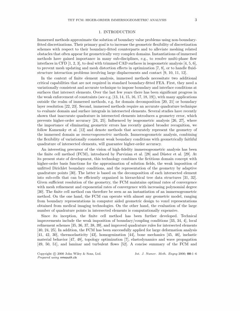
Figure 1: In the fictitious domain approach, the physical domain Ωphys is extended by the fictitiousdomain Ωfict into an embedding domain Ω that allows easy meshing. The original geometry isparameterized by a discontinuous indicator function α.

2.1. The fictitious domain approach

Figure 1 illustrates the fictitious domain concept that lies at the heart of the finite cell method.The physical domain of interest Ωphys, which can be geometrically complex, is extended by thefictitious domain Ωfict to an embedding domain Ω, which is geometrically simple. Analogousto standard finite element methods, we consider a variational formulation, which is definedover the complete embedding domain Ω. For example, in linear elasticity, we use the principleof virtual work

δW (u, δu) =

∫

Ω

σ : (∇sym δu) dV −

∫

Ω

δu · b dV −

∫

ΓN

δu · t dA = 0 (1)

where σ, b, u, δu and ∇sym denote the Cauchy stress tensor, body forces, displacement vector,test function and the symmetric part of the gradient, respectively [57, 58, 59]. Neumannboundary conditions are specified over the boundary of the embedding domain ∂Ω, wheretractions are zero by definition, and over ΓN of the physical domain, where tractions are givenby vector t (see Fig. 1). The elasticity tensor C [57, 58, 59] relating stresses and strains

σ = αC : ε (2)

is complemented by a scalar discontinuous indicator function

α (x)

= 1.0 ∀x ∈ Ωphys

≪ 1.0 ∀x ∈ Ωfict

(3)

which leaves the material parameters unchanged in the physical domain, but mitigates thecontribution of the fictitious domain in (2). In Ωfict, the value of the indicator function αshould be chosen as small as possible, but large enough to prevent extreme ill-conditioningof the stiffness matrix [29, 28]. In our experience, α can be set to zero for moderately highpolynomial degrees in the basis functions, e.g., quadratics or cubics. For high-order basisfunctions with p > 4 typical values of α range between 10−6 and 10−10.

2.2. Higher-order non-boundary-fitted meshes

Using a non-boundary-fitted grid of higher-order elements (see Fig. 1) kinematic quantitiesare discretized as

u =

n∑

a=1

Naua (4)



Finite cell mesh

k=0 k=1 k=2

k=3 k=4 k=5

with geometricboundary

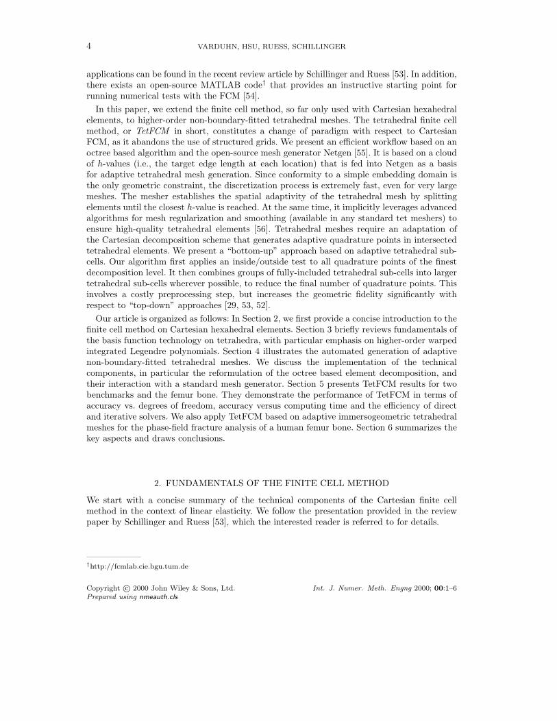
Figure 2: 2D sub-cell structure (thin blue lines) for adaptive integration of finite cells (bold black lines)intersected by a geometric boundary (dashed line).

δu =

n∑

a=1

Naδua (5)

The sum of Na denotes a finite set of n higher-order basis functions, and ua and δua are thecorresponding vector-valued unknown coefficients [60, 58]. The discretized displacements (4)and virtual displacements (5) are defined over the complete embedding domain. It is importantto identify basis functions with no support in the physical domain Ωphys and to remove themfrom the discretization, since they do not contribute to the accuracy of the approximation inΩphys, but lead to rows and columns filled with only zeros in the case of α = 0. Following thestandard Bubnov-Galerkin approach [57, 58, 59], the substitution of (4) and (5) into the weakform (1) leads to a discrete set of equations.

2.3. Adaptive quadrature based on recursive subdivision

The accuracy of numerical integration by Gauss quadrature [58, 61] assumes smoothness ofthe integrands that appear in the variational formulation (1). Standard Gauss quadrature cantherefore not be employed for integrating finite cells that are intersected by the geometricboundary, since the discontinuous indicator function α (3) introduces a discontinuity via (2).The Cartesian finite cell method based on quadrilateral and hexahedral meshes uses composedGauss quadrature to improve the integration accuracy in intersected elements, based on ahierarchical decomposition of each intersected element into integration sub-cells [29, 40].

We illustrate the sub-cell concept in Fig. 2 for the 2D case, where it can be implementedin the sense of a quadtree [31, 32]. On each sub-cell level, only those sub-cells intersectedby the geometric boundary are further subdivided. Subdivision is repeated until a predefinedmaximum depth is reached. The quadtree approach can be easily adjusted to binary trees oroctrees in 1D and 3D, respectively [29, 31, 32]. Finite elements are plotted in black andintegration sub-cells are plotted in blue lines throughout this work (see Fig. 2) for cleardistinction. The adaptive sub-cell scheme is easy to implement, but leads to an increasednumber of quadrature points, since in each sub-cell full Gauss quadrature is employed.



Interpreting the integration of intersected elements from a geometric point of view, adaptivequadrature enables the accurate representation of the geometry of the immersed domain. Onecan show that quadrature accuracy is equivalent to geometric accuracy, directly affecting thequality of the solution fields, an observation that was made for the first time in [24]. The abilityof composed Gauss quadrature to accurately represent the geometry by increasing the numberof sub-cells qualifies the FCM as an immersogeometric method [12].

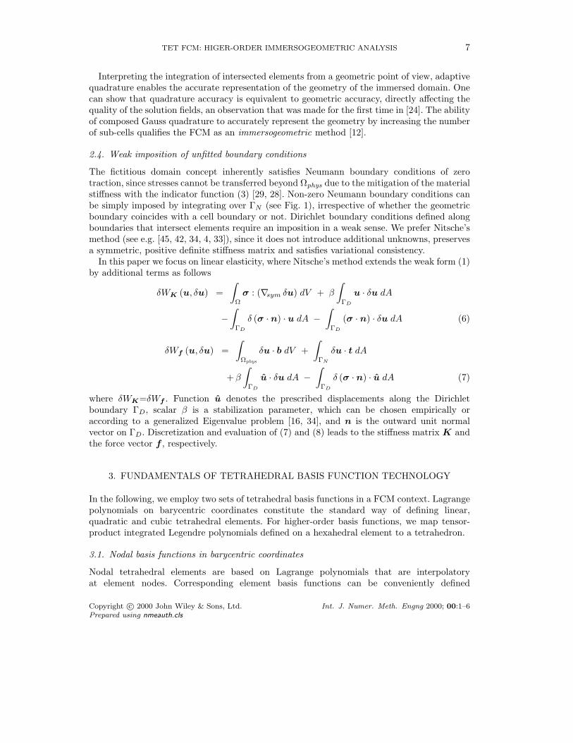
2.4. Weak imposition of unfitted boundary conditions

The fictitious domain concept inherently satisfies Neumann boundary conditions of zerotraction, since stresses cannot be transferred beyond Ωphys due to the mitigation of the materialstiffness with the indicator function (3) [29, 28]. Non-zero Neumann boundary conditions canbe simply imposed by integrating over ΓN (see Fig. 1), irrespective of whether the geometricboundary coincides with a cell boundary or not. Dirichlet boundary conditions defined alongboundaries that intersect elements require an imposition in a weak sense. We prefer Nitsche’smethod (see e.g. [45, 42, 34, 4, 33]), since it does not introduce additional unknowns, preservesa symmetric, positive definite stiffness matrix and satisfies variational consistency.

In this paper we focus on linear elasticity, where Nitsche’s method extends the weak form (1)by additional terms as follows

δWK (u, δu) =

∫

Ω

σ : (∇sym δu) dV + β

∫

ΓD

u · δu dA

−

∫

ΓD

δ (σ · n) · u dA −

∫

ΓD

(σ · n) · δu dA (6)

δWf (u, δu) =

∫

Ωphys

δu · b dV +

∫

ΓN

δu · t dA

+β

∫

ΓD

u · δu dA −

∫

ΓD

δ (σ · n) · u dA (7)

where δWK=δWf . Function u denotes the prescribed displacements along the Dirichletboundary ΓD, scalar β is a stabilization parameter, which can be chosen empirically oraccording to a generalized Eigenvalue problem [16, 34], and n is the outward unit normalvector on ΓD. Discretization and evaluation of (7) and (8) leads to the stiffness matrix K andthe force vector f , respectively.

3. FUNDAMENTALS OF TETRAHEDRAL BASIS FUNCTION TECHNOLOGY

In the following, we employ two sets of tetrahedral basis functions in a FCM context. Lagrangepolynomials on barycentric coordinates constitute the standard way of defining linear,quadratic and cubic tetrahedral elements. For higher-order basis functions, we map tensor-product integrated Legendre polynomials defined on a hexahedral element to a tetrahedron.

3.1. Nodal basis functions in barycentric coordinates

Nodal tetrahedral elements are based on Lagrange polynomials that are interpolatoryat element nodes. Corresponding element basis functions can be conveniently defined



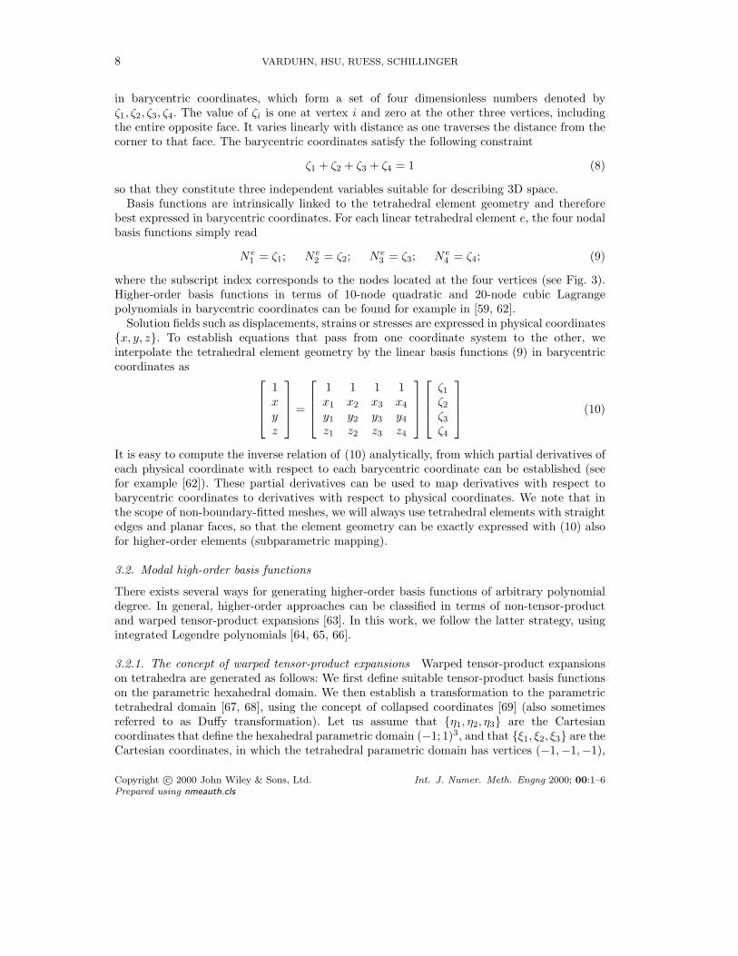
in barycentric coordinates, which form a set of four dimensionless numbers denoted byζ1, ζ2, ζ3, ζ4. The value of ζi is one at vertex i and zero at the other three vertices, includingthe entire opposite face. It varies linearly with distance as one traverses the distance from thecorner to that face. The barycentric coordinates satisfy the following constraint

ζ1 + ζ2 + ζ3 + ζ4 = 1 (8)

so that they constitute three independent variables suitable for describing 3D space.Basis functions are intrinsically linked to the tetrahedral element geometry and therefore

best expressed in barycentric coordinates. For each linear tetrahedral element e, the four nodalbasis functions simply read

Ne1 = ζ1; Ne

2 = ζ2; Ne3 = ζ3; Ne

4 = ζ4; (9)

where the subscript index corresponds to the nodes located at the four vertices (see Fig. 3).Higher-order basis functions in terms of 10-node quadratic and 20-node cubic Lagrangepolynomials in barycentric coordinates can be found for example in [59, 62].

Solution fields such as displacements, strains or stresses are expressed in physical coordinatesx, y, z. To establish equations that pass from one coordinate system to the other, weinterpolate the tetrahedral element geometry by the linear basis functions (9) in barycentriccoordinates as

1xyz

=

1 1 1 1x1 x2 x3 x4y1 y2 y3 y4z1 z2 z3 z4

ζ1ζ2ζ3ζ4

(10)

It is easy to compute the inverse relation of (10) analytically, from which partial derivatives ofeach physical coordinate with respect to each barycentric coordinate can be established (seefor example [62]). These partial derivatives can be used to map derivatives with respect tobarycentric coordinates to derivatives with respect to physical coordinates. We note that inthe scope of non-boundary-fitted meshes, we will always use tetrahedral elements with straightedges and planar faces, so that the element geometry can be exactly expressed with (10) alsofor higher-order elements (subparametric mapping).

3.2. Modal high-order basis functions

There exists several ways for generating higher-order basis functions of arbitrary polynomialdegree. In general, higher-order approaches can be classified in terms of non-tensor-productand warped tensor-product expansions [63]. In this work, we follow the latter strategy, usingintegrated Legendre polynomials [64, 65, 66].

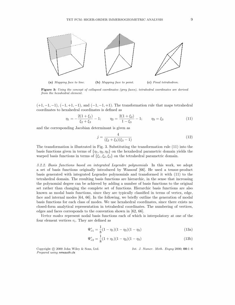
3.2.1. The concept of warped tensor-product expansions Warped tensor-product expansionson tetrahedra are generated as follows: We first define suitable tensor-product basis functionson the parametric hexahedral domain. We then establish a transformation to the parametrictetrahedral domain [67, 68], using the concept of collapsed coordinates [69] (also sometimesreferred to as Duffy transformation). Let us assume that η1, η2, η3 are the Cartesiancoordinates that define the hexahedral parametric domain (−1; 1)3, and that ξ1, ξ2, ξ3 are theCartesian coordinates, in which the tetrahedral parametric domain has vertices (−1,−1,−1),



(a) Mapping face to line. (b) Mapping face to point. (c) Final tetrahedron.

Figure 3: Using the concept of collapsed coordinates (grey faces), tetrahedral coordinates are derivedfrom the hexahedral element.

(+1,−1,−1), (−1,+1,−1), and (−1,−1,+1). The transformation rule that maps tetrahedralcoordinates to hexahedral coordinates is defined as

η1 = −2(1 + ξ1)

ξ2 + ξ3− 1; η2 =

2(1 + ξ2)

1− ξ3− 1; η3 = ξ3 (11)

and the corresponding Jacobian determinant is given as

j =4

(ξ2 + ξ3)(ξ3 − 1)(12)

The transformation is illustrated in Fig. 3. Substituting the transformation rule (11) into thebasis functions given in terms of η1, η2, η3 on the hexahedral parametric domain yields thewarped basis functions in terms of ξ1, ξ2, ξ3 on the tetrahedral parametric domain.

3.2.2. Basis functions based on integrated Legendre polynomials In this work, we adopta set of basis functions originally introduced by Wassouf [66]. He used a tensor-productbasis generated with integrated Legendre polynomials and transformed it with (11) to thetetrahedral domain. The resulting basis functions are hierarchic, in the sense that increasingthe polynomial degree can be achieved by adding a number of basis functions to the originalset rather than changing the complete set of functions. Hierarchic basis functions are alsoknown as modal basis functions, since they are typically classified in terms of vertex, edge,face and internal modes [64, 66]. In the following, we briefly outline the generation of modalbasis functions for each class of modes. We use hexahedral coordinates, since there exists noclosed-form analytical representation in tetrahedral coordinates. The numbering of vertices,edges and faces corresponds to the convention shown in [62, 66].

Vertex modes represent nodal basis functions each of which is interpolatory at one of thefour element vertices vi. They are defined as

Ψev1 =

1

8(1− η1)(1− η2)(1− η3) (13a)

Ψev2 =

1

8(1 + η1)(1− η2)(1− η3) (13b)



Ψev3 =

1

4(1 + η2)(1− η3) (13c)

Ψev4 =

1

2(1 + η3) (13d)

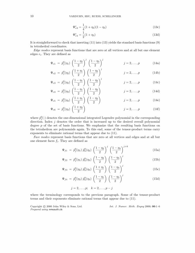
It is straightforward to check that inserting (11) into (13) yields the standard basis functions (9)in tetrahedral coordinates.Edge modes represent basis functions that are zero at all vertices and at all but one element

edges ei. They are defined as

Ψe1 = p0j (η1)

(

1− η22

)j (

1− η32

)j

j = 2, . . . , p (14a)

Ψe2 = p0j (η2)

(

1 + η12

) (

1− η32

)j

j = 2, . . . , p (14b)

Ψe3 = p0j (η2)

(

1− η12

) (

1− η32

)j

j = 2, . . . , p (14c)

Ψe4 = p0j (η3)

(

1− η12

) (

1− η22

)

j = 2, . . . , p (14d)

Ψe5 = p0j (η3)

(

1 + η12

) (

1− η22

)

j = 2, . . . , p (14e)

Ψe6 = p0j (η3)

(

1 + η22

)

j = 2, . . . , p (14f)

where p0j (·) denotes the one-dimensional integrated Legendre polynomial in the correspondingdirection. Index j denotes the order that is increased up to the desired overall polynomialdegree p of the set of basis functions. We emphasize that the resulting basis functions onthe tetrahedron are polynomials again. To this end, some of the tensor-product terms carryexponents to eliminate rational terms that appear due to (11).Face modes represent basis functions that are zero at all vertices and edges and at all but

one element faces fi. They are defined as

Ψf1 = p0j (η1) p0k(η2)

(

1− η22

)j (

1− η32

)j+k

(15a)

Ψf2 = p0j (η1) p0k(η3)

(

1− η22

) (

1− η32

)j

(15b)

Ψf3 = p0j (η2) p0k(η3)

(

1 + η12

) (

1− η32

)j

(15c)

Ψf4 = p0j (η2) p0k(η3)

(

1− η12

) (

1− η32

)j

(15d)

j = 2, . . . , p; k = 2, . . . , p− j

where the terminology corresponds to the previous paragraph. Some of the tensor-productterms and their exponents eliminate rational terms that appear due to (11).



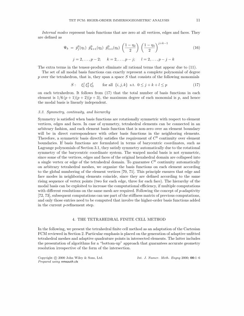
Internal modes represent basis functions that are zero at all vertices, edges and faces. Theyare defined as

Ψb = p0j (η1) p0k+1(η2) p0l+1(η3)

(

1− η22

) (

1− η32

)j+k−1

(16)

j = 2, . . . , p− 2; k = 2, . . . , p− j; l = 2, . . . , p− j − k

The extra terms in the tensor-product eliminate all rational terms that appear due to (11).The set of all modal basis functions can exactly represent a complete polynomial of degree

p over the tetrahedron, that is, they span a space S that consists of the following monomials

S : ξj1 ξk2 ξ

l3 for all i, j, k s.t. 0 ≤ j + k + l ≤ p (17)

on each tetrahedron. It follows from (17) that the total number of basis functions in eachelement is 1/6 (p + 1)(p + 2)(p + 3), the maximum degree of each monomial is p, and hencethe modal basis is linearly independent.

3.3. Symmetry, continuity, and hierarchy

Symmetry is satisfied when basis functions are rotationally symmetric with respect to elementvertices, edges and faces. In case of symmetry, tetrahedral elements can be connected in anarbitrary fashion, and each element basis function that is non-zero over an element boundarywill be in direct correspondence with other basis functions in the neighboring elements.Therefore, a symmetric basis directly satisfies the requirement of C0 continuity over elementboundaries. If basis functions are formulated in terms of barycentric coordinates, such asLagrange polynomials of Section 3.1, they satisfy symmetry automatically due to the rotationalsymmetry of the barycentric coordinate system. The warped modal basis is not symmetric,since some of the vertices, edges and faces of the original hexahedral domain are collapsed intoa single vertex or edge of the tetrahedral domain. To guarantee C0 continuity automaticallyon arbitrary tetrahedral meshes, we organize the basis functions on each element accordingto the global numbering of the element vertices [70, 71]. This principle ensures that edge andface modes in neighboring elements coincide, since they are defined according to the samerising sequence of vertex points (two for each edge, three for each face). The hierarchy of themodal basis can be exploited to increase the computational efficiency, if multiple computationswith different resolutions on the same mesh are required. Following the concept of p-adaptivity[72, 73], subsequent computations can use part of the stiffness matrix of previous computations,and only those entries need to be computed that involve the higher-order basis functions addedin the current p-refinement step.

4. THE TETRAHEDRAL FINITE CELL METHOD

In the following, we present the tetrahedral finite cell method as an adaptation of the CartesianFCM reviewed in Section 2. Particular emphasis is placed on the generation of adaptive unfittedtetrahedral meshes and adaptive quadrature points in intersected elements. The latter includesthe presentation of algorithms for a “bottom-up” approach that guarantees accurate geometryresolution irrespective of the form of the intersection.



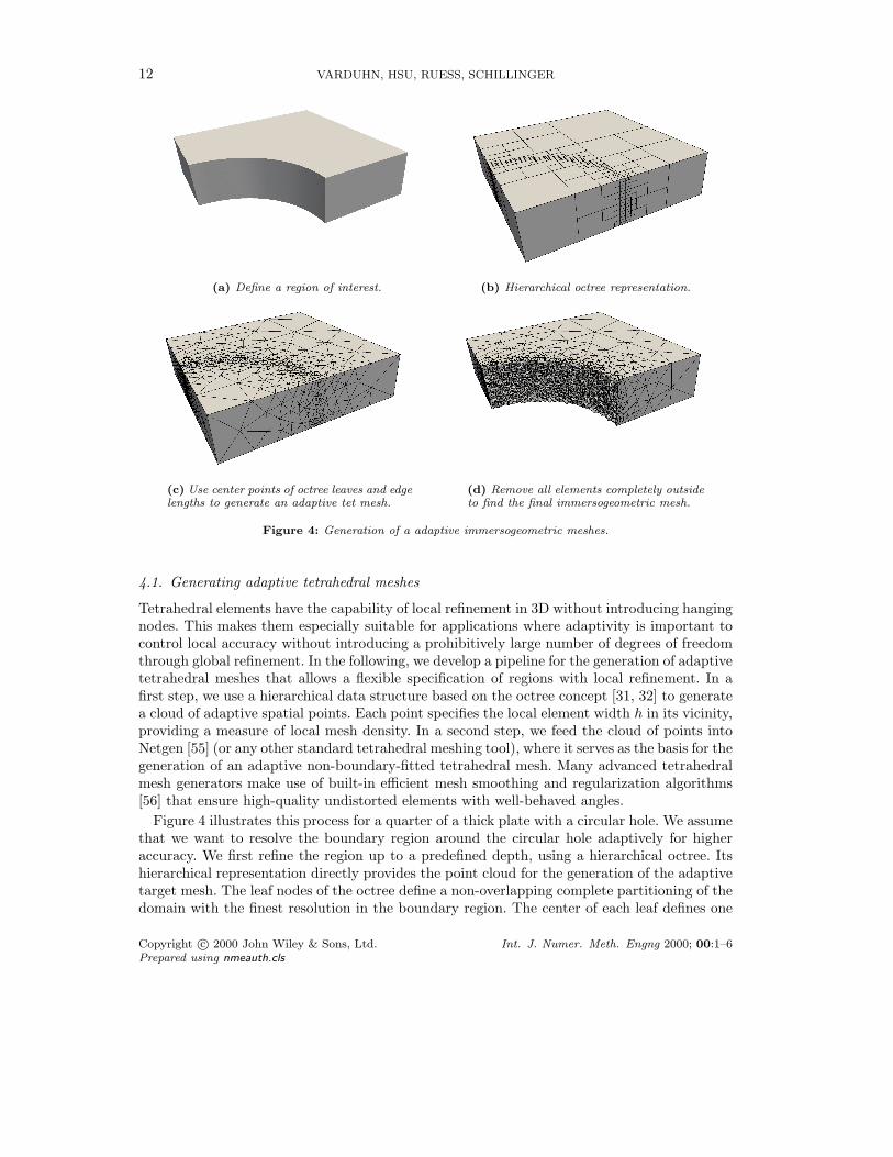
(a) Define a region of interest. (b) Hierarchical octree representation.

(c) Use center points of octree leaves and edgelengths to generate an adaptive tet mesh.

(d) Remove all elements completely outsideto find the final immersogeometric mesh.

Figure 4: Generation of a adaptive immersogeometric meshes.

4.1. Generating adaptive tetrahedral meshes

Tetrahedral elements have the capability of local refinement in 3D without introducing hangingnodes. This makes them especially suitable for applications where adaptivity is important tocontrol local accuracy without introducing a prohibitively large number of degrees of freedomthrough global refinement. In the following, we develop a pipeline for the generation of adaptivetetrahedral meshes that allows a flexible specification of regions with local refinement. In afirst step, we use a hierarchical data structure based on the octree concept [31, 32] to generatea cloud of adaptive spatial points. Each point specifies the local element width h in its vicinity,providing a measure of local mesh density. In a second step, we feed the cloud of points intoNetgen [55] (or any other standard tetrahedral meshing tool), where it serves as the basis for thegeneration of an adaptive non-boundary-fitted tetrahedral mesh. Many advanced tetrahedralmesh generators make use of built-in efficient mesh smoothing and regularization algorithms[56] that ensure high-quality undistorted elements with well-behaved angles.

Figure 4 illustrates this process for a quarter of a thick plate with a circular hole. We assumethat we want to resolve the boundary region around the circular hole adaptively for higheraccuracy. We first refine the region up to a predefined depth, using a hierarchical octree. Itshierarchical representation directly provides the point cloud for the generation of the adaptivetarget mesh. The leaf nodes of the octree define a non-overlapping complete partitioning of thedomain with the finest resolution in the boundary region. The center of each leaf defines one



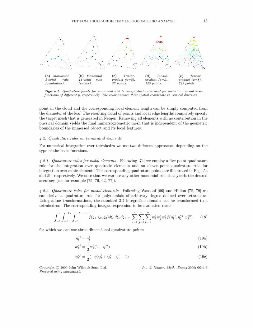
(a) Monomial5-point rule(quadratics).

(b) Monomial11-point rule(cubics).

(c) Tensor-product (p=2),27 points.

(d) Tensor-product (p=4),125 points.

(e) Tensor-product (p=8),729 points.

Figure 5: Quadrature points for monomial and tensor-product rules used for nodal and modal basisfunctions of different p, respectively. The color encodes their spatial coordinate in vertical direction.

point in the cloud and the corresponding local element length can be simply computed fromthe diameter of the leaf. The resulting cloud of points and local edge lengths completely specifythe target mesh that is generated in Netgen. Removing all elements with no contribution in thephysical domain yields the final immersogeometric mesh that is independent of the geometricboundaries of the immersed object and its local features.

4.2. Quadrature rules on tetrahedral elements

For numerical integration over tetrahedra we use two different approaches depending on thetype of the basis functions.

4.2.1. Quadrature rules for nodal elements Following [74] we employ a five-point quadraturerule for the integration over quadratic elements and an eleven-point quadrature rule forintegration over cubic elements. The corresponding quadrature points are illustrated in Figs. 5aand 5b, respectively. We note that we can use any other monomial rule that yields the desiredaccuracy (see for example [75, 76, 62, 77]).

4.2.2. Quadrature rules for modal elements Following Wassouf [66] and Hillion [78, 79] wecan derive a quadrature rule for polynomials of arbitrary degree defined over tetrahedra.Using affine transformations, the standard 3D integration domain can be transformed to atetrahedron. The corresponding integral expression to be evaluated reads

∫ 1

−1

∫ −ξ1

−1

∫ −ξ1−ξ2

−1

f(ξ1, ξ2, ξ3)dξ3dξ2dξ1 =

n∑

i=1

n∑

j=1

n∑

k=1

w∗iw

∗jw

∗kf(η

∗i1 , η

∗j2 , η

∗k3 ) (18)

for which we can use three-dimensional quadrature points

η∗i1 = ηi1 (19a)

w∗i1 =

1

2wi

1(1− η∗i1 ) (19b)

η∗j2 =1

2(−ηi1η

j2 + ηj2 − ηi1 − 1) (19c)



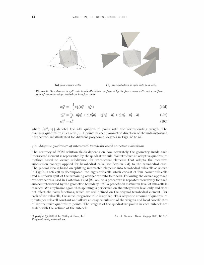
(a) four corner cells (b) an octahedron is split into four cells

Figure 6: One element is split into 8 subcells which are formed by the four corner cells and a uniformsplit of the remaining octahedron into four cells.

w∗j2 = −

1

2wj

2(η∗i1 + η∗j2 ) (19d)

η∗k3 =1

4(−ηi1η

k3 + ηi1η

j2η

k3 − ηj2η

k3 + ηk3 + ηi1η

j2 − ηj2 − 3) (19e)

w∗k3 = wk

3 (19f)

where η∗i, w∗i denotes the i-th quadrature point with the corresponding weight. The

resulting quadrature rules with p+1 points in each parametric direction of the untransformedhexahedron are illustrated for different polynomial degrees in Figs. 5c to 5e.

4.3. Adaptive quadrature of intersected tetrahedra based on octree subdivision

The accuracy of FCM solution fields depends on how accurately the geometry inside eachintersected element is represented by the quadrature rule. We introduce an adaptive quadraturemethod based on octree subdivision for tetrahedral elements that adapts the recursivesubdivision concept applied for hexahedral cells (see Section 2.3) to the tetrahedral case.The general idea is based on splitting intersected elements into tetrahedral sub-cells as shownin Fig. 6. Each cell is decomposed into eight sub-cells which consist of four corner sub-cellsand a uniform split of the remaining octahedron into four cells. Following the octree approachfor hexahedrals used in Cartesian FCM [29, 53], this procedure is repeated recursively for eachsub-cell intersected by the geometric boundary until a predefined maximum level of sub-cells isreached. We emphasize again that splitting is performed on the integration level only and doesnot affect the basis functions, which are still defined on the original tetrahedral element. Foreach of the sub-cells, the same integration rule is applied. This keeps the amount of quadraturepoints per sub-cell constant and allows an easy calculation of the weights and local coordinatesof the recursive quadrature points. The weights of the quadrature points in each sub-cell arescaled with the volume of the sub-cell.



From an algorithmic viewpoint, this idea is implemented in a “bottom-up” fashion. Insteadof building up the octree in the regular “top-down” approach, we first refine the completetetrahedron by generating the quadrature points of all possible leaves at the maximum treedepth. We then check each sub-cell whether it is intersected by the geometric boundary. Animportant consideration is how to determine best whether a sub-cell is intersected. Insteadof checking whether a face or edge is intersected or vertices are located on different sides ofthe geometric boundary, our intersection test solely relies on an inside/outside test for eachquadrature point. If we detect that quadrature points of one sub-cell are located on differentsides of the geometric boundary, we mark it as intersected. Based on this result, we startbuilding up the octree from the bottom up by combining sets of non-intersected leaves intoone leaf of higher level. This pruning procedure is repeated recursively until we reach theroot at the top, that is, the original finite element. The major advantage of the bottom-upapproach over the top-down approach is a significantly increased geometric accuracy, sinceelements that are intersected in such a way that only a small portion of their domain is cut arecaptured reliably. The bottom-up procedure is computationally more expensive than the top-down procedure, but is eminently suited for parallelization. A detailed algorithmic descriptionis provided in Algorithm 1.

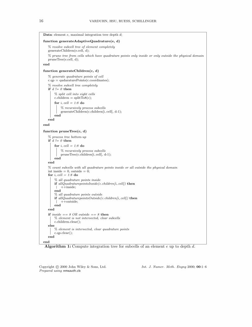
We illustrate the algorithm for the embedded cube in Fig. 7, which shows sub-cells fordifferent maximum octree depths. Our approach exhibits the following two advantages. First,we do not subdivide elements with very small cuts. In the top-down approach, they wouldbe subdivided, but without effect, since the corresponding quadrature points are all eithercompletely inside or outside of the physical domain. The bottom-up approach recombines allsub-cells to the original element, thus reducing the number of quadrature points and savingcomputation time. Second, we automatically exclude all elements that have only very smallportions of their element domain in the physical domain (created, e.g., by chopping off mostof the domain such that only one vertex of the tetrahedron is located within the physicaldomain). Such elements have no contribution to the system matrix, since no quadrature pointis located in the physical domain. If kept in the mesh, they either lead to a singular systemmatrix or negatively influence the condition of the system matrix, when a small value α ≪ 1is applied, see indicator function (3).

4.4. Voxel quadrature

Image based geometric models that emanate from medical imaging technologies such asquantitative computed tomography (qCT) scans are the most prominent data source forpatient-specific simulations in biomedical applications. They are made up of a rasterized voxelstructure, where each voxel contains a color value that can be associated with a physicalproperty, e.g., material density. If the tetrahedral finite cell method is applied for the analysis ofimage based geometric models, the concept of intersected elements and the recursive resolutionof the geometry by adaptive quadrature does not apply, as there exists no clearly definedboundary of the physical domain. Instead, we suggest a quadrature approach that follows twoprinciples. First, tetrahedral elements that are completely located outside the physical domain,that is, the color value of all voxel located within this element are below or above the predefinedthreshold, are removed from the mesh. Second, we subdivide each tetrahedral element intosub-cells. The level of sub-cells is the same for each cell and throughout the complete mesh.The sub-cell resolution is chosen such that the density of the resulting quadrature points



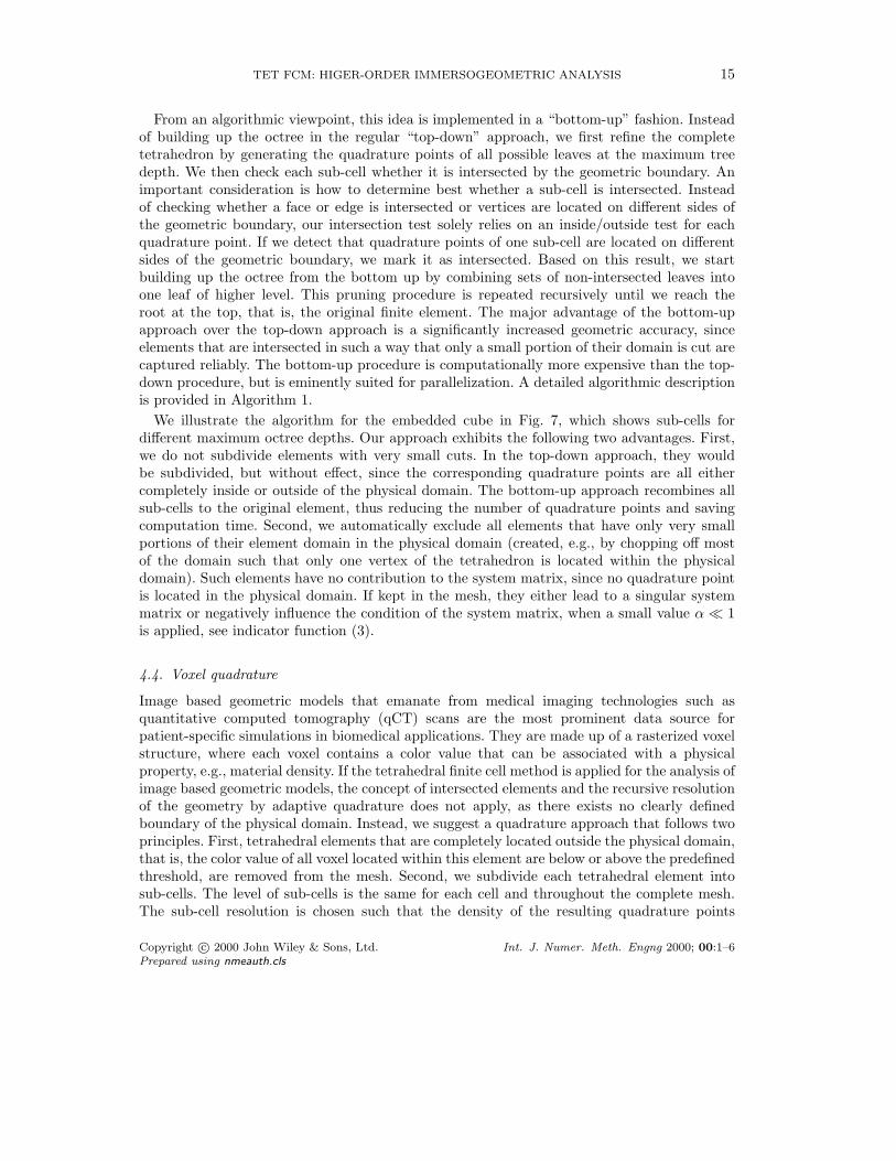
Data: element e, maximal integration tree depth d;

function generateAdaptiveQuadrature(e, d)

% resolve subcell tree of element completelygenerateChildren(e.cell, d);

% prune tree from cells which have quadrature points only inside or only outside the physical domainpruneTree(e.cell, d);

end

function generateChildren(c, d)

% generate quadrature points of cellc.qp = qudaraturePoints(c.coordinates);

% resolve subcell tree completelyif d != 0 then

% split cell into eight cellsc.children = splitTo8(c);

for i cell = 1:8 do

% recursively process subcellsgenerateChildren(c.children[i cell], d-1);

endend

end

function pruneTree(c, d)

% process tree bottom-upif d != 0 then

for i cell = 1:8 do

% recursively process subcellspruneTree(c.children[i cell], d-1);

endend

% count subcells with all quadrature points inside or all outside the physical domainint inside = 0, outside = 0;for i cell = 1:8 do

% all quadrature points insideif allQuadraturepointsInside(c.children[i cell]) then

++inside;end% all quadrature points outsideif allQuadraturepointsOutside(c.children[i cell]) then

++outside;end

end

if inside == 8 OR outside == 8 then% element is not intersected, clear subcellsc.children.clear();

else% element is intersected, clear quadrature pointsc.qp.clear();

end

end

Algorithm 1: Compute integration tree for subcells of an element e up to depth d.



(a) Non-boundary-fitted mesh of a cube (elements in black, sub-tetrahedra in blue, boundary in white).

(b) level d = 0 (c) level d = 1 (d) level d = 2 (e) level d = 3 (f) level d = 4

Figure 7: By building the tree from the bottom up, we ensure that any small cut that can be resolvedby the finest level d of sub-cells is captured. The color indicates for each sub-cell how many quadraturepoints are located inside the cube domain.

approximately corresponds to the voxel density. As a consequence, each quadrature point canbe approximately associated with one voxel. We emphasize that a finer resolution of quadraturepoints should be avoided, as it could resolve sharp interfaces between single voxels, which arean artifact of the geometric model.

5. NUMERICAL EXAMPLES

In this section we examine the accuracy and computational efficiency of the tetrahedral finitecell method for several benchmark problems. In particular, we illustrate the ability of high-



order modal basis functions to achieve exponential convergence rates and the advantages ofquadratic and cubic nodal basis functions in terms of reasonable conditioning and fast iterativesolution of large systems. We also highlight the ability of immersogeometric tetrahedral meshesto locally refine the solution fields in three dimensions.

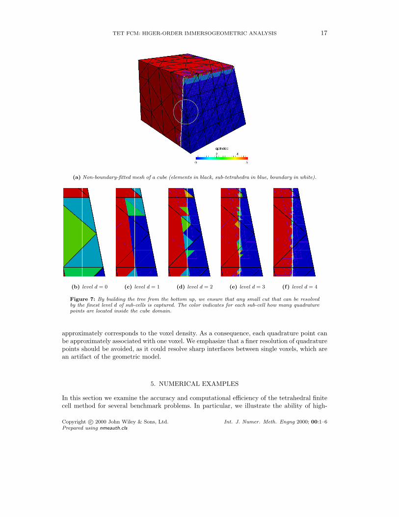
5.1. Thick plate with a circular hole

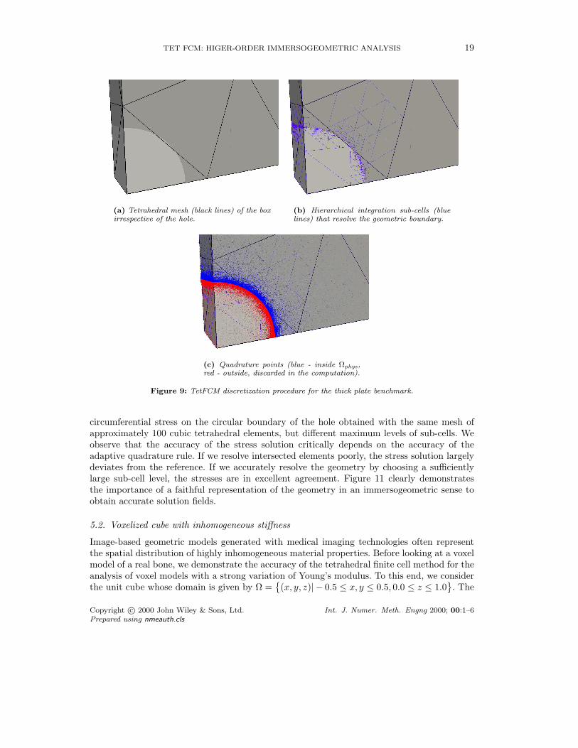
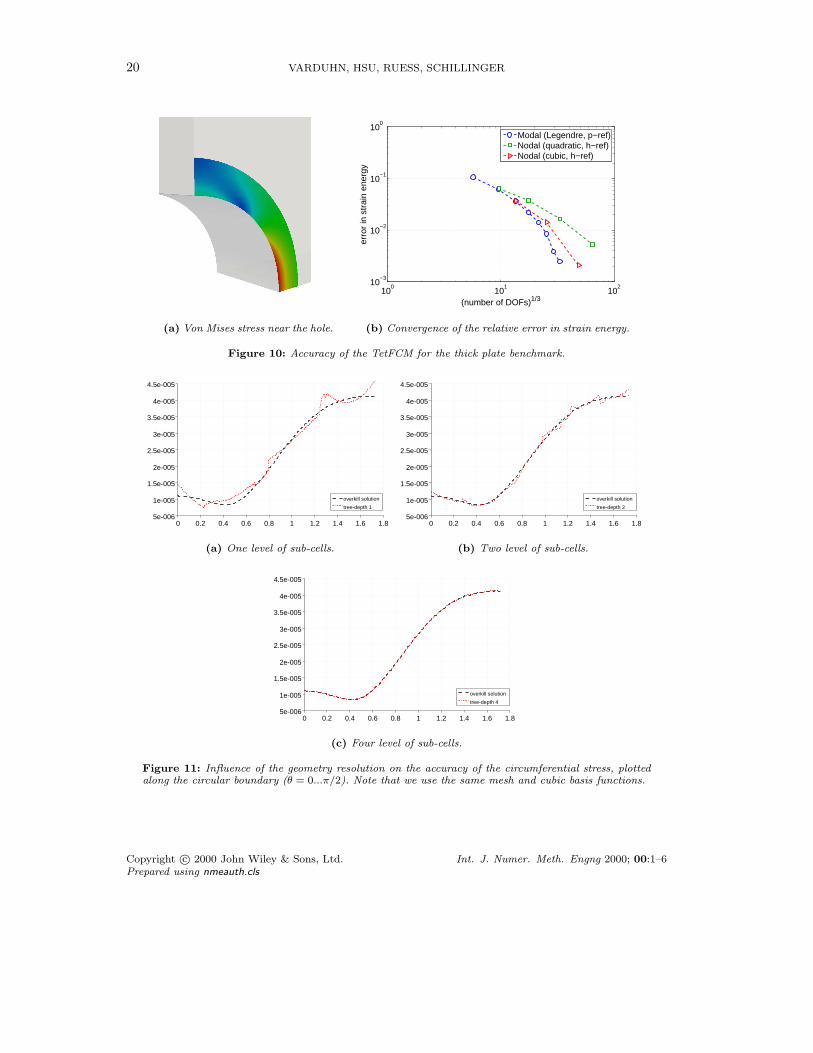
As a first benchmark, we consider a thick plate with a circular hole under uniform tension shownin Fig. 8. We make use of the symmetry of the problem, reducing the system to one octantof the original domain. Symmetry boundary conditions are applied in a weak sense by usingNitsche’s method. Figure 9 illustrates the basic steps of the immersogeometric discretizationprocedure using the TetFCM scheme. First, we generate an unfitted tetrahedral mesh of theembedding domain, using the mesh generator Netgen. Second, we employ octree subdivisiondescribed in Section 4.3 to generate integration sub-cells for performing adaptive quadraturein intersected elements.Figure 10a plots the von Mises stress distribution in the boundary region close to the circular

boundary. We observe that the stress field is smooth, the concentration at the lower boundarycan be captured accurately and no unphysical interference of the boundary can be detected.We also compute the relative error in strain energy norm defined as [58, 64, 59]

er =

√

|Unum − Uref |

Uref

(20)

where Unum represents the numerical strain energy obtained for a specific discretization, andUref is a reference strain energy computed with an overkill discretization. Figure 10b plots theenergy error versus the total number of degrees of freedom. We employ a series of uniformlyrefined Cartesian meshes with quadratic and cubic Lagrange basis functions and a coarse meshbased on integrated Legendre basis functions, where we increase the polynomial degree p atfixed element size. The geometry in intersected elements is resolved by adaptive quadraturewith six levels of hierarchical sub-cells. We observe that for h-refinement with quadraticand cubic basis functions, we achieve optimal rates of convergence, which correspond to thepolynomial degree p. For p-refinement, the TetFCM achieves exponential rates.The stress accuracy that can be achieved directly on the immersed boundary in intersected

elements is of particular interest in many situations, e.g., for stress analysis, where maximumstresses mostly occur on the surface, or in coupled multi-physics problems, where surfacequantities need to be exchanged between different solvers. Figures 11a to 11c plot the

Sym. BC

L=10L=10

R=1

Sym. BC

h=1Sym. BC

E=100,000

ν=0.3

Material:

Traction t=10

Figure 8: Three-dimensional thick plate with a circular hole.



(a) Tetrahedral mesh (black lines) of the boxirrespective of the hole.

(b) Hierarchical integration sub-cells (bluelines) that resolve the geometric boundary.

(c) Quadrature points (blue - inside Ωphys,red - outside, discarded in the computation).

Figure 9: TetFCM discretization procedure for the thick plate benchmark.

circumferential stress on the circular boundary of the hole obtained with the same mesh ofapproximately 100 cubic tetrahedral elements, but different maximum levels of sub-cells. Weobserve that the accuracy of the stress solution critically depends on the accuracy of theadaptive quadrature rule. If we resolve intersected elements poorly, the stress solution largelydeviates from the reference. If we accurately resolve the geometry by choosing a sufficientlylarge sub-cell level, the stresses are in excellent agreement. Figure 11 clearly demonstratesthe importance of a faithful representation of the geometry in an immersogeometric sense toobtain accurate solution fields.

5.2. Voxelized cube with inhomogeneous stiffness

Image-based geometric models generated with medical imaging technologies often representthe spatial distribution of highly inhomogeneous material properties. Before looking at a voxelmodel of a real bone, we demonstrate the accuracy of the tetrahedral finite cell method for theanalysis of voxel models with a strong variation of Young’s modulus. To this end, we considerthe unit cube whose domain is given by Ω =

(x, y, z)| − 0.5 ≤ x, y ≤ 0.5, 0.0 ≤ z ≤ 1.0

. The



(a) Von Mises stress near the hole.

100

101

102

10−3

10−2

10−1

100

(number of DOFs)1/3

erro

r in

str

ain

ener

gy

Modal (Legendre, p−ref)Nodal (quadratic, h−ref)Nodal (cubic, h−ref)

(b) Convergence of the relative error in strain energy.

Figure 10: Accuracy of the TetFCM for the thick plate benchmark.

5e-006

1e-005

1.5e-005

2e-005

2.5e-005

3e-005

3.5e-005

4e-005

4.5e-005

0 0.2 0.4 0.6 0.8 1 1.2 1.4 1.6 1.8

overkill solution

tree-depth 1

(a) One level of sub-cells.

5e-006

1e-005

1.5e-005

2e-005

2.5e-005

3e-005

3.5e-005

4e-005

4.5e-005

0 0.2 0.4 0.6 0.8 1 1.2 1.4 1.6 1.8

overkill solution

tree-depth 2

(b) Two level of sub-cells.

5e-006

1e-005

1.5e-005

2e-005

2.5e-005

3e-005

3.5e-005

4e-005

4.5e-005

0 0.2 0.4 0.6 0.8 1 1.2 1.4 1.6 1.8

overkill solution

tree-depth 4

(c) Four level of sub-cells.

Figure 11: Influence of the geometry resolution on the accuracy of the circumferential stress, plottedalong the circular boundary (θ = 0...π/2). Note that we use the same mesh and cubic basis functions.



inhomogeneous Young’s modulus is given by the function

E(x, y, z) = 3x(10 + sin(5y))(50 + cos(10z)) (21)

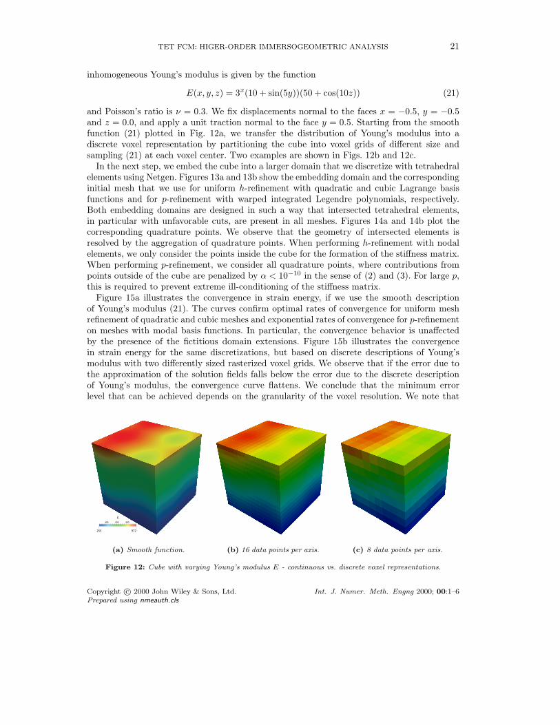
and Poisson’s ratio is ν = 0.3. We fix displacements normal to the faces x = −0.5, y = −0.5and z = 0.0, and apply a unit traction normal to the face y = 0.5. Starting from the smoothfunction (21) plotted in Fig. 12a, we transfer the distribution of Young’s modulus into adiscrete voxel representation by partitioning the cube into voxel grids of different size andsampling (21) at each voxel center. Two examples are shown in Figs. 12b and 12c.In the next step, we embed the cube into a larger domain that we discretize with tetrahedral

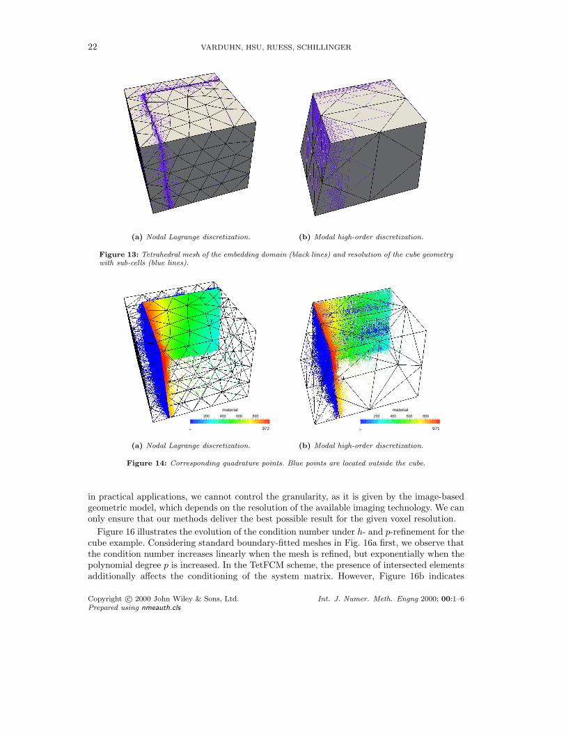
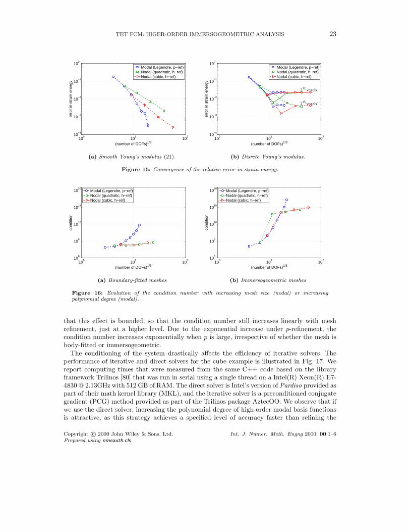
elements using Netgen. Figures 13a and 13b show the embedding domain and the correspondinginitial mesh that we use for uniform h-refinement with quadratic and cubic Lagrange basisfunctions and for p-refinement with warped integrated Legendre polynomials, respectively.Both embedding domains are designed in such a way that intersected tetrahedral elements,in particular with unfavorable cuts, are present in all meshes. Figures 14a and 14b plot thecorresponding quadrature points. We observe that the geometry of intersected elements isresolved by the aggregation of quadrature points. When performing h-refinement with nodalelements, we only consider the points inside the cube for the formation of the stiffness matrix.When performing p-refinement, we consider all quadrature points, where contributions frompoints outside of the cube are penalized by α < 10−10 in the sense of (2) and (3). For large p,this is required to prevent extreme ill-conditioning of the stiffness matrix.Figure 15a illustrates the convergence in strain energy, if we use the smooth description

of Young’s modulus (21). The curves confirm optimal rates of convergence for uniform meshrefinement of quadratic and cubic meshes and exponential rates of convergence for p-refinementon meshes with modal basis functions. In particular, the convergence behavior is unaffectedby the presence of the fictitious domain extensions. Figure 15b illustrates the convergencein strain energy for the same discretizations, but based on discrete descriptions of Young’smodulus with two differently sized rasterized voxel grids. We observe that if the error due tothe approximation of the solution fields falls below the error due to the discrete descriptionof Young’s modulus, the convergence curve flattens. We conclude that the minimum errorlevel that can be achieved depends on the granularity of the voxel resolution. We note that

255

E

800600400

972

(a) Smooth function. (b) 16 data points per axis. (c) 8 data points per axis.

Figure 12: Cube with varying Young’s modulus E - continuous vs. discrete voxel representations.



(a) Nodal Lagrange discretization. (b) Modal high-order discretization.

Figure 13: Tetrahedral mesh of the embedding domain (black lines) and resolution of the cube geometrywith sub-cells (blue lines).

0

material800600400200

972

(a) Nodal Lagrange discretization.

0

material800600400200

971

(b) Modal high-order discretization.

Figure 14: Corresponding quadrature points. Blue points are located outside the cube.

in practical applications, we cannot control the granularity, as it is given by the image-basedgeometric model, which depends on the resolution of the available imaging technology. We canonly ensure that our methods deliver the best possible result for the given voxel resolution.

Figure 16 illustrates the evolution of the condition number under h- and p-refinement for thecube example. Considering standard boundary-fitted meshes in Fig. 16a first, we observe thatthe condition number increases linearly when the mesh is refined, but exponentially when thepolynomial degree p is increased. In the TetFCM scheme, the presence of intersected elementsadditionally affects the conditioning of the system matrix. However, Figure 16b indicates



100

101

102

10−4

10−3

10−2

10−1

100

(number of DOFs)1/3

erro

r in

str

ain

ener

gy


(a) Smooth Young’s modulus (21).

100

101

102

10−4

10−3

10−2

10−1

100

(number of DOFs)1/3

erro

r in

str

ain

ener

gy

212 voxels

215 voxels


(b) Disrete Young’s modulus.

Figure 15: Convergence of the relative error in strain energy.

100

101

102

100

105

1010

1015

1020

(number of DOFs)1/3

cond

ition


(a) Boundary-fitted meshes

100

101

102

100

105

1010

1015

1020

(number of DOFs)1/3

cond

ition


(b) Immersogeometric meshes

Figure 16: Evolution of the condition number with increasing mesh size (nodal) or increasingpolynomial degree (modal).

that this effect is bounded, so that the condition number still increases linearly with meshrefinement, just at a higher level. Due to the exponential increase under p-refinement, thecondition number increases exponentially when p is large, irrespective of whether the mesh isbody-fitted or immersogeometric.The conditioning of the system drastically affects the efficiency of iterative solvers. The

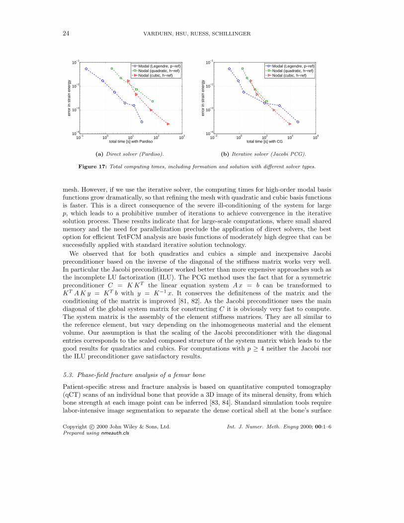
performance of iterative and direct solvers for the cube example is illustrated in Fig. 17. Wereport computing times that were measured from the same C++ code based on the libraryframework Trilinos [80] that was run in serial using a single thread on a Intel(R) Xeon(R) E7-4830 @ 2.13GHz with 512 GB of RAM. The direct solver is Intel’s version of Pardiso provided aspart of their math kernel library (MKL), and the iterative solver is a preconditioned conjugategradient (PCG) method provided as part of the Trilinos package AztecOO. We observe that ifwe use the direct solver, increasing the polynomial degree of high-order modal basis functionsis attractive, as this strategy achieves a specified level of accuracy faster than refining the



10−1

100

101

102

103

10−4

10−3

10−2

10−1

total time [s] with Pardiso

erro

r in

str

ain

ener

gy


(a) Direct solver (Pardiso).

10−2

100

102

104

106

10−4

10−3

10−2

10−1

total time [s] with CG

erro

r in

str

ain

ener

gy


(b) Iterative solver (Jacobi PCG).

Figure 17: Total computing times, including formation and solution with different solver types.

mesh. However, if we use the iterative solver, the computing times for high-order modal basisfunctions grow dramatically, so that refining the mesh with quadratic and cubic basis functionsis faster. This is a direct consequence of the severe ill-conditioning of the system for largep, which leads to a prohibitive number of iterations to achieve convergence in the iterativesolution process. These results indicate that for large-scale computations, where small sharedmemory and the need for parallelization preclude the application of direct solvers, the bestoption for efficient TetFCM analysis are basis functions of moderately high degree that can besuccessfully applied with standard iterative solution technology.

We observed that for both quadratics and cubics a simple and inexpensive Jacobipreconditioner based on the inverse of the diagonal of the stiffness matrix works very well.In particular the Jacobi preconditioner worked better than more expensive approaches such asthe incomplete LU factorization (ILU). The PCG method uses the fact that for a symmetricpreconditioner C = KKT the linear equation system Ax = b can be transformed toKT AK y = KT b with y = K−1 x. It conserves the definiteness of the matrix and theconditioning of the matrix is improved [81, 82]. As the Jacobi preconditioner uses the maindiagonal of the global system matrix for constructing C it is obviously very fast to compute.The system matrix is the assembly of the element stiffness matrices. They are all similar tothe reference element, but vary depending on the inhomogeneous material and the elementvolume. Our assumption is that the scaling of the Jacobi preconditioner with the diagonalentries corresponds to the scaled composed structure of the system matrix which leads to thegood results for quadratics and cubics. For computations with p ≥ 4 neither the Jacobi northe ILU preconditioner gave satisfactory results.

5.3. Phase-field fracture analysis of a femur bone

Patient-specific stress and fracture analysis is based on quantitative computed tomography(qCT) scans of an individual bone that provide a 3D image of its mineral density, from whichbone strength at each image point can be inferred [83, 84]. Standard simulation tools requirelabor-intensive image segmentation to separate the dense cortical shell at the bone’s surface



from the foam-like trabecular bone in the interior. The finite cell method provides a frameworkthat seamlessly integrates qCT data into automatic stress and fracture analysis [53, 45].

5.3.1. Phase-field model for brittle fracture Our test problem is based on a phase-field modelfor brittle fracture [85, 86, 87, 88, 89], which is represented in variational form for quasistaticconditions by the following coupled equations

∫(

4l0ψ+0

Gc

+ 1

)

c q dΩ +

∫

4l20 ∇c ∇q dΩ =

∫

q dΩ (22)

∫

(

σ+ + σ−)

: ∇w dΩ =

∫

b ·w dΩ+

∫

t ·w d∂Ω (23)

The pairs u,w and c, q represent the displacement and phase-field solutions andcorresponding test functions, Gc and l0 are the energy release rate and a length scale, andλ and µ are the Lame parameters. The tensile and compressive parts of the stress tensor read

σ+ := c2(

λ 〈tr(ε)〉+I + 2µ ε+

)

(24)

σ− := λ 〈tr(ε)〉−

I + 2µ ε− (25)

which are based on an additive split of the strain tensor. The phase-field part (22) requireshomogeneous Neumann boundary conditions, the elasticity part (23) the usual traction anddisplacement constraints.

The basic idea of the phase-field fracture model (22) and (23) is to represent cracks by acontinuous scalar field c that has a value of one away from the crack and is zero at the cracklocation. The phase-field serves as a multiplication factor to tensile energy components in (24)such that it locally penalizes the capability of the material to carry tensile stress at the cracklocation. In this sense, the phase-field idea is conceptually very similar to the fictitious domainapproach applied in the finite cell method. The diffusiveness of the crack approximation iscontrolled by the length-scale parameter l0. The diffusive approximation of the crack by acontinuous phase-field eliminates the need for explicit discontinuities in the mesh. Cracks canbe represented independently from the mesh and its topology by the solution of an additionaldifferential equation that completely determines crack nucleation and propagation. The phase-field fracture approach has proven to accurately and robustly capture crack behavior in twoand three dimensions for quasi-static fracture [90, 91, 92, 93, 87], dynamic crack propagation[94, 92, 95, 96, 97, 98], at finite strains [99], for fracture in piezo- and ferroelectric materials[100, 101, 102] and for cohesive fracture [103, 104].

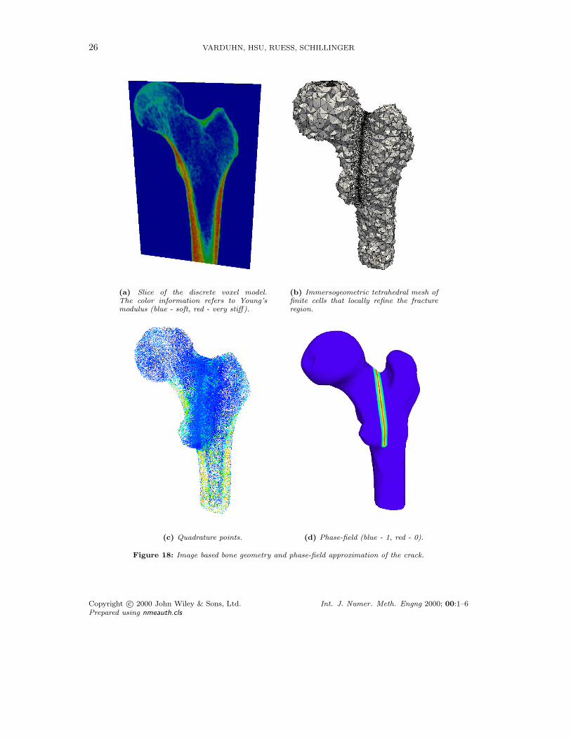
5.3.2. TetFCM with local refinement As the phase-field approximation exhibits sharp localgradients near the crack and is otherwise constant, local refinement is mandatory for anefficient phase-field analysis technology. In the following, we demonstrate the advantages ofthe tetrahedral finite cell method in terms of highly graded meshes that adaptively refine thecrack region in the context of image based stress analysis of a human femur bone. Our analysisis based on a qCT scan of the bone, which can be transferred into the distribution of Young’smodulus over the bone [83], and a homogeneous Poisson’s ratio ν = 0.3. Figure 18a shows a



(a) Slice of the discrete voxel model.The color information refers to Young’smodulus (blue - soft, red - very stiff).

(b) Immersogeometric tetrahedral mesh offinite cells that locally refine the fractureregion.

(c) Quadrature points. (d) Phase-field (blue - 1, red - 0).

Figure 18: Image based bone geometry and phase-field approximation of the crack.



slice of the discrete voxel model‡. We use the strain energy based method shown in [88, 89]to impose a crack through the central shaft of the bone. We generate a cloud of h-valuesusing the octree based approach of Section 4.1, where we make use of the assumed local strainenergy to drive the depth of the octree. Based on the cloud of h-values we generate an adaptiveimmersogeometric tetrahedral mesh of the bone, shown in Fig. 18b. The target element sizeclose to the crack location is twice the length parameter l0 of the phase-field model. Furtheraway from the crack, we allow a significantly larger element size. As described in Section 4.4,we remove all elements that do not have at least one voxel with Young’s modulus above aminimum threshold within their support. The quadrature points are shown in Fig. 18c.

Homogeneous Neumann boundary conditions in the phase-field part (22) over the bonesurface are automatically imposed without surface quadrature in the TetFCM scheme. Inthe elasticity part (23), we apply a load of 1000 N on the bone head over a circular area.Displacement boundary conditions at the bone’s distal face are weakly enforced with Nitsche’smethod. To perform quadrature for the formation of matrix and vector components, wetriangulate these surfaces. Figure 18d plots the phase-field solution that approximates thesharp crack. A uniform tetrahedral mesh of the bone with an equivalent resolution of thephase-field would yield 250 million degrees of freedom, as compared to approximately 500,000

‡Courtesy of Prof. Zohar Yosibash, Dept. of Mechanical Engineering, Ben-Gurion University, Beer-Sheva, Israel;http://www.bgu.ac.il/∼zohary/

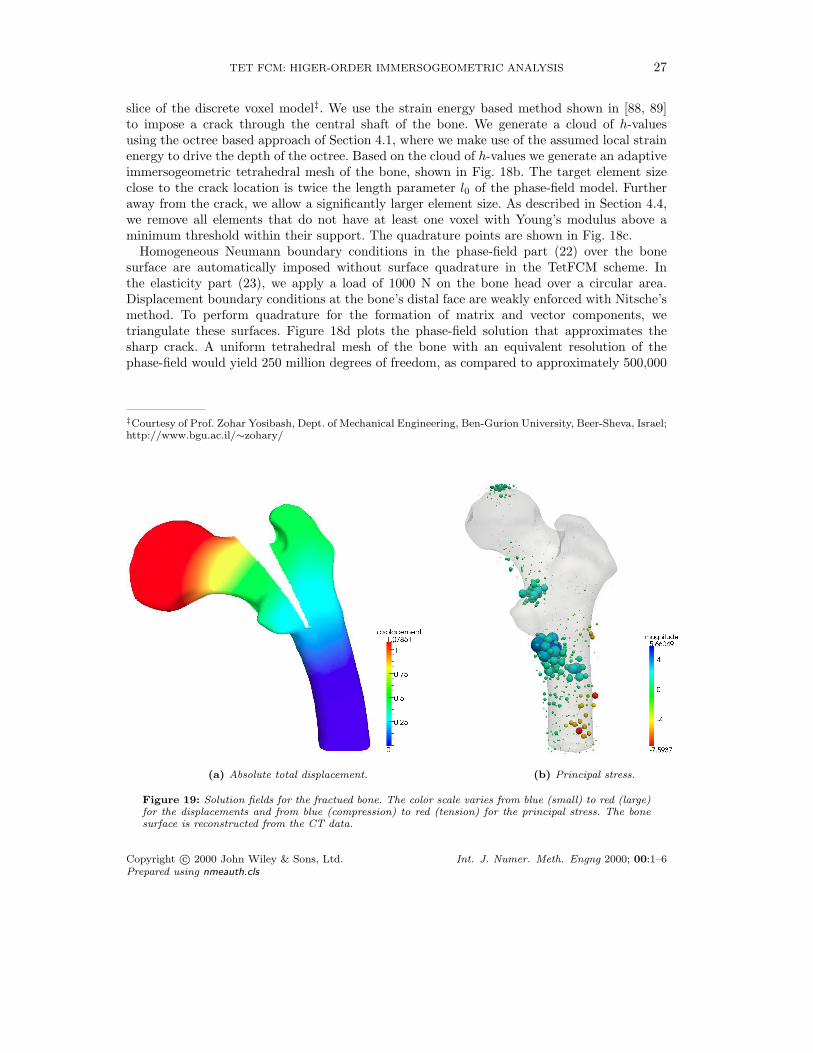
(a) Absolute total displacement. (b) Principal stress.

Figure 19: Solution fields for the fractued bone. The color scale varies from blue (small) to red (large)for the displacements and from blue (compression) to red (tension) for the principal stress. The bonesurface is reconstructed from the CT data.



degrees of freedom of the present adaptive mesh. We then solve the elasticity problem, usingthe phase-field solution in (24). In Figs. 19a and 19b, we plot the total displacement and theprincipal stress distribution. We observe that maximum stresses appear due to the bendingeffect in the area where the crack reduces the effective height.

6. SUMMARY AND CONCLUSIONS

In this paper, we extended the finite cell method, so far only used with Cartesian hexahedralelements, to higher-order non-boundary-fitted tetrahedral meshes. With respect to CartesianFCM, the TetFCM scheme requires three basic adaptations. First, the notion of a Cartesianmesh is abandoned and replaced by the more flexible notion of a general unstructuredtetrahedral mesh of the embedding domain. We encouraged the use of open-source meshingtools such as Netgen, in particular for exploiting advanced algorithms for mesh regularizationand smoothing that ensure high-quality tetrahedral elements. According to our experience,meshing is extremely fast, even for very large meshes, since there are no geometric constraintsother than the simple boundaries of the embedding domain. We also outlined an efficientworkflow based on an octree based algorithm for obtaining locally refined tetrahedral meshes.Second, tetrahedral basis functions, for example based on standard quadratic and cubicLagrange polynomials or based on high-order warped integrated Legendre polynomials, areused. Third, we presented a modification of the Cartesian sub-cell quadrature scheme thatachieves accurate integration of intersected tetrahedral elements by increasing quadraturepoints near the geometric boundary. In particular, we demonstrated that building the tree“from the bottom up” automatically guarantees a high fidelity resolution of the geometry withthe finest level of sub-cells available.Using a series of 3D numerical examples with smooth solutions, we demonstrated that

TetFCM yields optimal rates of convergence, when the mesh is refined, and exponential rates,when the polynomial degree of the basis is increased. To illustrate the fundamental importanceof accurate geometry resolution, we plotted the stress solution over the immersed boundaryfor different levels of the integration sub-cells. Using the same tetrahedral mesh with the samebasis functions, an analysis with poor geometry resolution of intersected elements resulted insignificant errors in boundary stresses, while an analysis with several levels of adaptive sub-cells resulted in very accurate boundary stresses that were indistinguishable from the referencesolution. Furthermore, our numerical tests indicated that p-refinement based on the increase ofthe polynomial degree is computationally more efficient than analysis based on mesh refinementat a fixed polynomial degree, when we use a direct solver. However, our numerical tests alsoindicated that the decay in conditioning of the discrete system that occurs due to unfavorablycut elements is bounded for mesh refinement at moderate polynomial degrees, but deteriorateswithout bounds for p-refinement. As a consequence, we could successfully apply an iterativePCG solver for quadratic and cubic meshes, but encountered prohibitive numbers of iterationsfor high polynomial degrees. The TetFCM is a suitable tool for problems where local refinementis mandatory for efficiency. As an example, we presented an image based phase-field fractureanalysis of a human femur bone, where we adaptively resolved sharp gradients in the diffusephase-field approximation of the crack.In our view, TetFCM constitutes another opportunity for immersogeometric analysis. It

provides access to the advantages of adaptive tetrahedral meshes in the FCM context. From



an analysis point of view, TetFCM does not perform better than Cartesian FCM, and it ismerely the choice and preference of the analyst, which FCM scheme is used. TetFCM couldalso bring us closer to the adoption of FCM capabilities into a commercial FEA package,since adaptive higher-order tetrahedral elements and tetrahedral mesh generators are alreadyavailable in most commercial production codes.

ACKNOWLEDGEMENTS

We acknowledge the Minnesota Supercomputing Institute (MSI) of the University of Minnesota forproviding computing resources that have contributed to the research results reported within thispaper (https://www.msi.umn.edu/). We thank Dr. Sascha Duczek (Otto-von-Guericke UniversityMagdeburg) for helpful comments and discussions.



REFERENCES

1. S. Haeri and J.S. Shrimpton. On the application of immersed boundary, fictitious domain and body-conformal mesh methods to many particle multiphase flows. International Journal of Multiphase Flow,40:38–55, 2012.

2. A. Calderer, S. Kang, and F. Sotiropoulos. Level set immersed boundary method for coupled simulation ofair/water interaction with complex floating structures. Journal of Computational Physics, 277:201–227,2014.

3. B. Avci and P. Wriggers. Direct numerical simulation of particulate flows using a fictitious domainmethod. In Numerical Simulations of Coupled Problems in Engineering, pages 105–127. Springer, 2014.

4. M. Ruess, D. Schillinger, A.I. Ozcan, and E. Rank. Weak coupling for isogeometric analysis ofnon-matching and trimmed multi-patch geometries. Computer Methods in Applied Mechanics andEngineering, 269:46–71, 2014.

5. A.P. Nagy and D.J. Benson. On the numerical integration of trimmed isogeometric elements. ComputerMethods in Applied Mechanics and Engineering, 284:165–185, 2015.

6. M. Breitenberger, A. Apostolatos, B. Philipp, R. Wuchner, and K.-U. Bletzinger. Analysis in computeraided design: Nonlinear isogeometric b-rep analysis of shell structures. Computer Methods in AppliedMechanics and Engineering, 284:401–457, 2015.

7. J. Parvizian, A. Duster, and E. Rank. Topology optimization using the finite cell method. Optimizationand Engineering, 13:57–78, 2012.

8. J. Benk, H.-J. Bungartz, M. Mehl, and M. Ulbrich. Immersed boundary methods for fluid-structureinteraction and shape optimization within an FEM-based PDE toolbox. In Advanced Computing, pages25–56. Springer, 2013.

9. I. Borazjani, L. Ge, and F. Sotiropoulos. Curvilinear immersed boundary method for simulating fluidstructure interaction with complex 3D rigid bodies. Journal of Computational Physics, 227(16):7587–7620, 2008.

10. M.-C. Hsu, D. Kamensky, Y. Bazilevs, M.S. Sacks, and T.J.R. Hughes. Fluid–structure interactionanalysis of bioprosthetic heart valves: significance of arterial wall deformation. Computational Mechanics,54(4):1055–1071, 2014.

11. F. Sotiropoulos and X. Yang. Immersed boundary methods for simulating fluid–structure interaction.Progress in Aerospace Sciences, 65:1–21, 2014.

12. D. Kamensky, M.-C. Hsu, D. Schillinger, J. A. Evans, A. Aggarwal, Y. Bazilevs, M. S. Sacks, andT. J. R. Hughes. An immersogeometric variational framework for fluid–structure interaction: applicationto bioprosthetic heart valves. Computer Methods in Applied Mechanics and Engineering, 284:1005–1053,2015.

13. B.I. Wohlmuth. Discretization techniques based on domain decomposition. Lecture Notes inComputational Science and Engineering, Vol. 17, 2001.

14. A. Hansbo and P. Hansbo. An unfitted finite element method, based on Nitsche’s method, for ellipticinterface problems. Computer Methods in Applied Mechanics and Engineering, 191:537–552, 2002.

15. S. Fernandez-Mendez and A. Huerta. Imposing essential boundary conditions in mesh-free methods.Computer Methods in Applied Mechanics and Engineering, 193:1257–1275, 2004.

16. A. Embar, J. Dolbow, and I. Harari. Imposing Dirichlet boundary conditions with Nitsche’s method andspline-based finite elements. International Journal for Numerical Methods in Engineering, 83:877–898,2010.

17. C. Annavarapu, M. Hautefeuille, and J.E. Dolbow. A robust Nitsche’s formulation for interface problems.Computer Methods in Applied Mechanics and Engineering, 225:44–54, 2012.

18. I. Harari and E. Grosu. A unified approach for embedded boundary conditions for fourth-order ellipticproblems. International Journal for Numerical Methods in Engineering, accepted for publication, 2014.

19. Y. Guo and M. Ruess. Nitsche’s method for a coupling of isogeometric thin shells and blended shellstructures. Computer Methods in Applied Mechanics and Engineering, 284:881–905, 2015.

20. R. Becker, P. Hansbo, and R. Stenberg. A finite element method for domain decomposition with non-matching grids. Mathematical Modelling and Numerical Analysis, 37(2):209–225, 2003.

21. A. Apostolatos, R. Schmidt, R. Wuchner, and K.-U. Bletzinger. A Nitsche-type formulation andcomparison of the most common domain decomposition methods in isogeometric analysis. InternationalJournal for Numerical Methods in Engineering, 97(7):473–504, 2014.

22. Y. Bazilevs and T.J.R. Hughes. Weak imposition of Dirichlet boundary conditions in fluid mechanics.Computers & Fluids, 36:12–26, 2007.

23. M.C. Hsu, I. Akkerman, and Y. Bazilevs. Wind turbine aerodynamics using ALE-VMS: validation andthe role of weakly enforced boundary conditions. Computational Mechanics, 50:499–511, 2012.

24. A. Stavrev. The role of higher-order geometry approximation and accurate quadrature in NURBS basedimmersed boundary methods. Master Thesis, Technische Universitat Munchen, 2012.



25. L. Kudela. Highly Accurate Subcell Integration in the Context of The Finite Cell Method. Master Thesis,Technische Universitat Munchen, 2013.

26. T.J.R. Hughes, J.A. Cottrell, and Y. Bazilevs. Isogeometric analysis: CAD, finite elements, NURBS, exactgeometry and mesh refinement. Computer Methods in Applied Mechanics and Engineering, 194:4135–4195, 2005.

27. J.A. Cottrell, T.J.R. Hughes, and Y. Bazilevs. Isogeometric analysis: Towards Integration of CAD andFEA. John Wiley & Sons, 2009.

28. J. Parvizian, A. Duster, and E. Rank. Finite cell method: h- and p- extension for embedded domainmethods in solid mechanics. Computational Mechanics, 41:122–133, 2007.

29. A. Duster, J. Parvizian, Z. Yang, and E. Rank. The finite cell method for three-dimensional problemsof solid mechanics. Computer Methods in Applied Mechanics and Engineering, 197:3768–3782, 2010.

30. D. Schillinger. The p- and B-spline versions of the geometrically nonlinear finite cell method andhierarchical refinement strategies for adaptive isogeometric and embedded domain analysis. Dissertation,Technische Universitat Munchen, http://d-nb.info/103009943X/34, 2012.

31. H. Samet. The design and analysis of spatial data structures, volume 199. Addison-Wesley Reading,MA, 1990.

32. H. Samet. Foundations of Multidimensional and Metric Data Structures. Morgan Kaufmann Publishers,2006.

33. N. Zander. The Finite Cell Method for linear thermoelasticity. Master Thesis, Technische UniversitatMunchen, 2011.

34. M. Ruess, D. Schillinger, Y. Bazilevs, V. Varduhn, and E. Rank. Weakly enforced essential boundaryconditions for NURBS-embedded and trimmed NURBS geometries on the basis of the finite cell method.International Journal for Numerical Methods in Engineering, 95(10):811–846, 2013.

35. D. Schillinger and E. Rank. An unfitted hp adaptive finite element method based on hierarchical B-splinesfor interface problems of complex geometry. Computer Methods in Applied Mechanics and Engineering,200(47–48):3358–3380, 2011.

36. D. Schillinger, A. Duster, and E. Rank. The hp-d adaptive finite cell method for geometrically nonlinearproblems of solid mechanics. International Journal for Numerical Methods in Engineering, 89:1171–1202,2012.

37. D. Schillinger, L. Dede’, M.A. Scott, J.A. Evans, M.J. Borden, E. Rank, and T.J.R. Hughes. Anisogeometric design-through-analysis methodology based on adaptive hierarchical refinement of NURBS,immersed boundary methods, and T-spline CAD surfaces. Computer Methods in Applied Mechanics andEngineering, 249-250:116–150, 2012.

38. M. Joulaian and A. Duster. Local enrichment of the finite cell method for problems with materialinterfaces. Computational Mechanics, 52:741–762, 2013.

39. N. Zander, T. Bog, S. Kollmannsberger, D. Schillinger, and E. Rank. Multi-Level hp-Adaptivity: High-Order mesh adaptivity without the difficulties of constraining hanging nodes. Computational Mechanics,accepted for publication, 2015.

40. Z. Yang, M. Ruess, S. Kollmannsberger, A. Duster, and E. Rank. An efficient integration techniquefor the voxel-based finite cell method. International Journal for Numerical Methods in Engineering,91:457–471, 2012.

41. D. Schillinger, S. Kollmannsberger, R.-P. Mundani, and E. Rank. The finite cell method for geometricallynonlinear problems of solid mechanics. IOP Conference Series: Material Science and Engineering,10:012170, 2010.

42. D. Schillinger, M. Ruess, N. Zander, Y. Bazilevs, A. Duster, and E. Rank. Small and large deformationanalysis with the p- and B-spline versions of the Finite Cell Method. Computational Mechanics,50(4):445–478, 2012.

43. N. Zander, S. Kollmannsberger, M. Ruess, Z. Yosibash, and E. Rank. The Finite Cell Method for linearthermoelasticity. Computers & Mathematics with Applications, 64(11):3527–3541, 2012.

44. A. Duster, H.-G. Sehlhorst, and E. Rank. Numerical homogenization of heterogeneous and cellularmaterials utilizing the finite cell method. Computational Mechanics, 50:413–431, 2012.

45. M. Ruess, D. Tal, N. Trabelsi, Z. Yosibash, and E. Rank. The finite cell method for bone simulations:Verification and validation. Biomechanics and Modeling in Mechanobiology, 11(3):425–437, 2012.

46. C.V. Verhoosel, G.J. van Zwieten, B. van Rietbergen, and R. de Borst. Image-based goal-orientedadaptive isogeometric analysis with application to the micro-mechanical modeling of trabecular bone.Computer Methods in Applied Mechanics and Engineering, 284:138–164, 2015.

47. A. Abedian, J. Parvizian, A. Duster, and E. Rank. The finite cell method for the J2 flow theory ofplasticity. Finite Elements in Analysis and Design, 69:37–47, 2013.

48. M. Ranjbar, M. Mashayekhi, J. Parvizian, A. Duster, and E. Rank. Using the finite cell method topredict crack initiation in ductile materials. Computational Materials Science, 82:427 – 434, 2014.

49. C. Willberg, S. Duczek, J.M. Vivar Perez, D. Schmicker, and U. Gabbert. Comparison of different higher



order finite element schemes for the simulation of Lamb waves. Computer Methods in Applied Mechanicsand Engineering, 241–244:246–261, 2012.

50. S Duczek, M Joulaian, A Duster, and U Gabbert. Numerical analysis of lamb waves using the finite andspectral cell methods. International Journal for Numerical Methods in Engineering, 99(1):26–53, 2014.

51. M. Joulaian, S. Duczek, U. Gabbert, and A. Duster. Finite and spectral cell method for wave propagationin heterogeneous materials. Computational Mechanics, 54(1):661–675, 2014.

52. F. Xu, D. Schillinger, D. Kamensky, V. Varduhn, C. Wang, and M.-C. Hsu. The tetrahedral finite cellmethod for fluids: Immersogeometric analysis of turbulent flow around complex geometries. Submittedto Computer & Fluids, 2015.

53. D. Schillinger and M. Ruess. The Finite Cell Method: A review in the context of higher-order structuralanalysis of CAD and image-based geometric models. Archives of Computational Methods in Engineering,doi:10.1007/s11831-014-9115-y, 2014.

54. N. Zander, T. Bog, M. Elhaddad, R. Espinoza, H. Hu, A.F. Joly, C. Wu, P. Zerbe, A. Duster,S. Kollmannsberger, J. Parvizian, M. Ruess, D. Schillinger, and E. Rank. FCMLab: A finite cell researchtoolbox for MATLAB. Advances in Engineering Software, 74:49–63,, 2014.

55. Netgen Mesh Generator, developed by j. schoeberl, http://sourceforge.net/projects/netgen-mesher/,2015.

56. Joachim Schoberl. NETGEN. An advancing front 2D/3D-mesh generator based on abstract rules.Computing and Visualization in Science, 1(1):41–52, 1997.

57. K.-J. Bathe. Finite Element Procedures. Prentice-Hall, 1996.58. T.J.R. Hughes. The Finite Element Method: Linear Static and Dynamic Finite Element Analysis. Dover

Publications, 2000.59. O.C. Zienkiewicz and R.L. Taylor. The Finite Element Method – The Basis, volume 1. Butterworth-

Heinemann, 6th edition, 2005.60. J. Bonet and R. Wood. Nonlinear Continuum Mechanics for Finite Element Analysis. Cambridge

University Press, 2008.61. E. Suli and D.F. Mayers. An introduction to numerical analysis. Cambridge University Press, 2003.62. C. Felippa. Advanced finite element methods. Course notes, available online at

http://www.colorado.edu/engineering/CAS/courses.d/AFEM.d/Home.html.63. C. Canuto, M.Y. Hussaini, A. Quarteroni, and T.A. Zang. Spectral Methods: Fundamentals in Single

Domains. Springer, 2006.64. B. Szabo and I. Babuska. Finite Element Analysis. Wiley, 1991.65. A. Duster, H. Broker, and E. Rank. The p-version of the finite element method for three-dimensional

curved thin walled structures. International Journal for Numerical Methods in Engineering, 52:673–703,2001.

66. Z. Wassouf. Die Mortar Methode fur Finite Elemente hoher Ordnung. Dissertation, TechnischeUniversitat Munchen, 2010.

67. M. Dubiner. Spectral methods on triangles and other domains. Journal of Scientific Computing,6(4):345–390, 1991.

68. S.J. Sherwin and G.E. Karniadakis. A new triangular and tetrahedral basis for high-order (hp) finiteelement methods. International Journal for Numerical Methods in Engineering, 38(22):3775–3802, 1995.

69. G.E. Karniadakis and S.J. Sherwin. Spectral/hp Element Methods for Computational Fluid Dynamics.Oxford University Press, 2005.

70. T.C. Warburton, S.J. Sherwin, and G.E. Karniadakis. Basis functions for triangular and quadrilateralhigh-order elements. SIAM Journal on Scientific Computing, 20(5):1671–1695, 1999.

71. Timothy Warburton. Spectral/hp methods on polymorphic multidomains: Algorithms and applications,1999.

72. B.A. Szabo, A. Duster, and E. Rank. The p-version of the Finite Element Method. In E. Stein,R. de Borst, and T. J. R. Hughes, editors, Encyclopedia of Computational Mechanics, volume 1, chapter 5,pages 119–139. John Wiley & Sons, 2004.

73. Zohar Yosibash. p-fems in biomechanics: Bones and arteries. Computer Methods in Applied Mechanicsand Engineering, 249:169–184, 2012.

74. P. Keast. Moderate-degree tetrahedral quadrature formulas. Computer Methods in Applied Mechanicsand Engineering, 55:339–348, 1986.

75. A. Stroud. Approximate Calculation of Multiple Integrals. Prentice Hall, 1971.76. R. Cools. Monomial cubature rules since “Stroud”: A compilation - Part 2. Journal of Computational

and Applied Mathematics, 112(1):21–27, 1999.77. D. Schillinger, S.J. Hossain, and T.J.R. Hughes. Reduced Bezier element quadrature rules for quadratic

and cubic splines in isogeometric analysis. Computer Methods in Applied Mechanics and Engineering,277:1–45, 2014.

78. P. Hillion. Numerical integration on a triangle. International Journal for Numerical Methods in



Engineering, 11:797–815, 1977.79. P. Hillion. Numerical integration on a tetrahedron. Calcolo, 18(2):117–130, 1979.80. Trilinos Version 11.12, Sandia National Laboratories, http://trilinos.org/, 2015.81. Y. Saad. Iterative methods for sparse linear systems. Society for Industrial and Applied Mathematics,

2003.82. G.H. Golub and C. Van Loan. Matrix Computations. Johns Hopkins University Press, 1996.83. J.H. Keyak and Y. Falkinstein. Comparison of in situ and in vitro CT scan-based finite element model

predictions of proximal femoral fracture load. Medical Engineering & Physics, 25(9):781–787, 2003.84. N. Trabelsi, Z. Yosibash, and C. Milgrom. Validation of subject-specific automated p-fe analysis of the

proximal femur. Journal of Biomechanics, 42(3):234–241, 2009.85. G.A. Francfort and J.-J. Marigo. Revisiting brittle fracture as an energy minimization problem. Journal

of the Mechanics and Physics of Solids, 46(8):1319–1342, 1998.86. B. Bourdin, G.A. Francfort, and J.-J. Marigo. The variational approach to fracture. Journal of Elasticity,

91(1-3):5–148, 2008.87. C. Miehe, M. Hofacker, and F. Welschinger. A phase field model for rate-independent crack propagation:

Robust algorithmic implementation based on operator splits. Computer Methods in Applied Mechanicsand Engineering, 199(45):2765–2778, 2010.

88. M.J. Borden, M.A. Scott, J.A. Evans, and T.J.R. Hughes. Isogeometric finite element data structuresbased on Bezier extraction of NURBS. International Journal for Numerical Methods in Engineering,87:15–47, 2011.

89. D. Schillinger, M.J. Borden, and H.K. Stolarski. Isogeometric collocation for phase-field fracture models.Computer Methods in Applied Mechanics and Engineering, 284:583–610, 2015.

90. G. Lancioni and G.F. Royer-Carfagni. The variational approach to fracture mechanics. A practicalapplication to the French Pantheon in Paris. Journal of Elasticity, 95(1-2):1–30, 2009.

91. C. Kuhn and R. Muller. A continuum phase field model for fracture. Engineering Fracture Mechanics,77(18):3625–3634, 2010.

92. M.J. Borden, C.V. Verhoosel, M.A. Scott, Hughes T.J.R., and C.M. Landis. A phase-field descriptionof dynamic brittle fracture. Computer Methods in Applied Mechanics and Engineering, 217–220:77–95,2012.

93. C. Miehe, F. Welschinger, and M. Hofacker. Thermodynamically consistent phase-field models of fracture:Variational principles and multi-field FE implementations. International Journal for Numerical Methodsin Engineering, 83(10):1273–1311, 2010.

94. M.J. Borden, T.J.R. Hughes, C.M. Landis, and C.V. Verhoosel. A higher-order phase-field model forbrittle fracture: Formulation and analysis within the isogeometric analysis framework. Computer Methodsin Applied Mechanics and Engineering, 273:100 – 118, 2014.

95. B. Bourdin, C.J. Larsen, and C.L. Richardson. A time-discrete model for dynamic fracture based oncrack regularization. International Journal of Fracture, 168(2):133–143, 2011.

96. M. Hofacker and C. Miehe. Continuum phase field modeling of dynamic fracture: variational principlesand staggered FE implementation. International Journal of Fracture, 178(1-2):113–129, 2012.

97. M. Hofacker and C. Miehe. A phase field model of dynamic fracture: Robust field updates for the analysisof complex crack patterns. International Journal for Numerical Methods in Engineering, 93(3):276–301,2013.

98. A. Schluter, A. Willenbucher, C. Kuhn, and R. Muller. Phase field approximation of dynamic brittlefracture. Computational Mechanics, 2014.

99. C. Miehe and L.-M. Schanzel. Phase field modeling of fracture in rubbery polymers. part i: Finiteelasticity coupled with brittle failure. Journal of the Mechanics and Physics of Solids, 65:93–113, 2014.

100. C. Miehe, F. Welschinger, and M. Hofacker. A phase field model of electromechanical fracture. Journalof the Mechanics and Physics of Solids, 58(10):1716–1740, 2010.

101. Z.A. Wilson, M.J. Borden, and C.M. Landis. A phase-field model for fracture in piezoelectric ceramics.International Journal of Fracture, 183(2):135–153, 2013.

102. A. Abdollahi and I. Arias. Phase-field modeling of fracture in ferroelectric materials. Archives ofComputational Methods in Engineering, doi:10.1007/s11831-014-9118-8, 2014.

103. C.V. Verhoosel and R. de Borst. A phase-field model for cohesive fracture. International Journal forNumerical Methods in Engineering, 96(1):43–62, 2013.

104. J. Vignollet, S. May, R. de Borst, and C.V. Verhoosel. Phase-field models for brittle and cohesive fracture.Meccanica, doi:10.1007/s11012-013-9862-0, 2014.


Documents

Varduhn, V., Hsu, M.-C., Ruess, M., and …eprints.gla.ac.uk/116058/1/116058.pdfVarduhn, V., Hsu, M.-C., Ruess, M., and Schillinger, D. (2016) The tetrahedral finite cell method: higher