VaR Methods

IEF 217a: Lecture Section 6

Fall 2002

Jorion, Chapter 9 (skim)

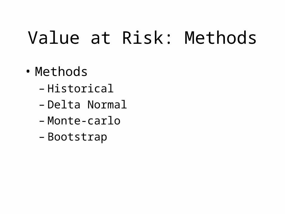
Value at Risk: Methods

• Methods– Historical– Delta Normal– Monte-carlo– Bootstrap

Historical

• Use past data to build histograms

• Method:– Gather historical prices/returns– Use this data to predict possible moves in the

portfolio over desired horizon of interest

Delta Normal

• Estimate means and standard deviations• Use normal approximations• What if value is a function V(s)?• Need to estimate derivatives (see Jorion)• Computer handles this automatically in

monte-carlo• Also, derivatives are all local

approximations

Monte-Carlo VaR

• Make assumptions about distributions• Simulate random variables• matlab: mcdow.m• Results similar to delta normal• Why bother with monte-carlo?

– Nonnormal distributions– More complicated portfolios and risk measures– Confidence intervals: mcdow2.m

Value at Risk: Methods

• Methods– Historical– Delta Normal– Monte-carlo– Bootstrapping

Bootstrapping

• Historical/Monte-carlo hybrid

• We’ve done this already– data = [5 3 -6 9 0 4 6 ];– sample(data,n);

• Example– bdow.m

Harder Example

• Foreign currency forward contract

• 91 day forward

• 91 days in the future– Firm receives 10 million BP (British Pounds)– Delivers 15 million US $

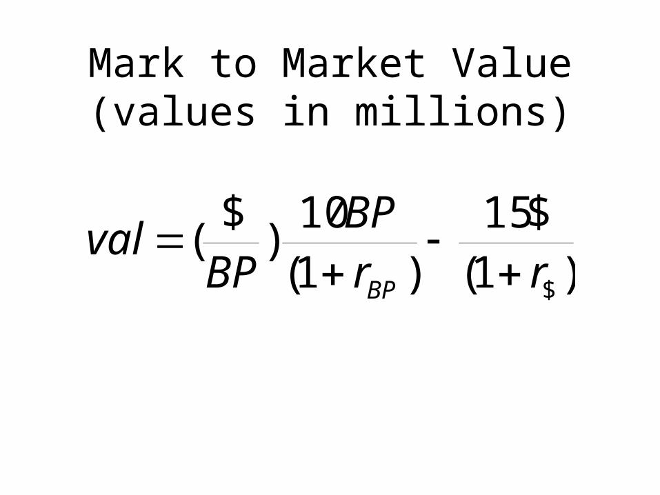
Mark to Market Value(values in millions)

)1($15

)1(10

)$

($rr

BPBP

valBP

Risk Factors

• Exchange rate ($/BP)• r(BP): British interest rate• r($): US interest rate• Assume:

– ($/BP) = 1.5355– r(BP) = 6% per year– r($) = 5.5% per year– Effective interest rate = (days to maturity/360)r

Find the 5%, 1 Day VaR

• Very easy solution– Assume the interest rates are constant

• Analyze VaR from changes in the exchange rate price on the portfolio

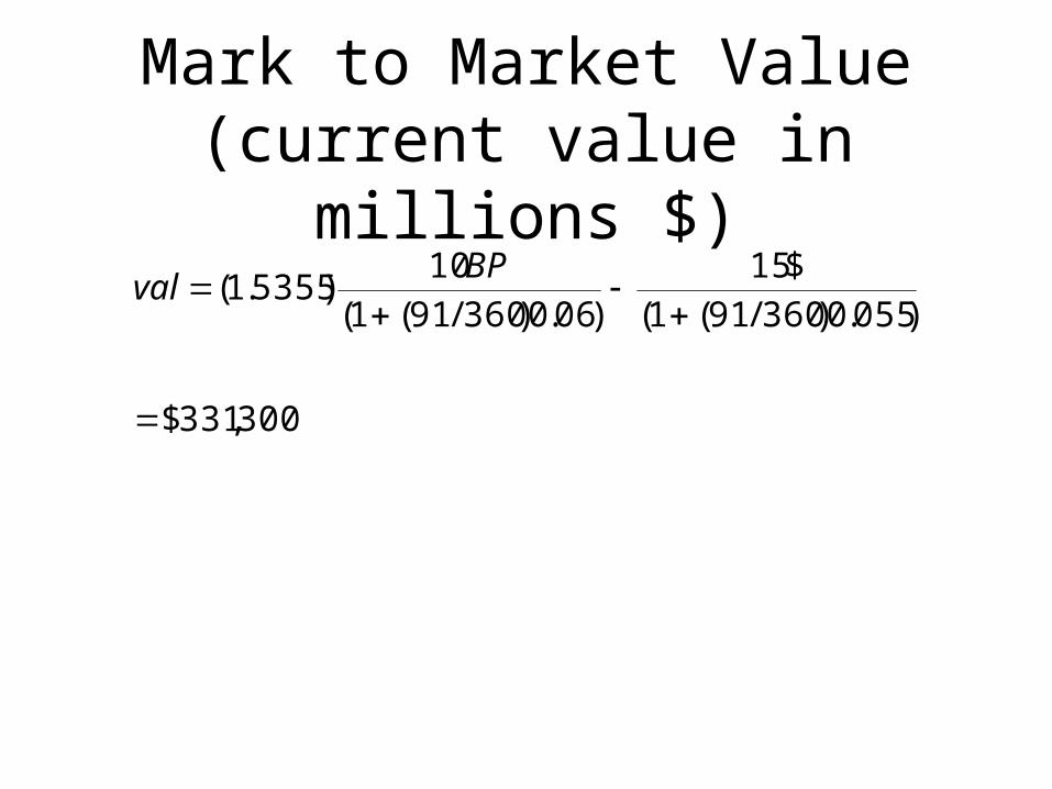
Mark to Market Value(current value in millions $)

300,331$

)055.0)360/91(1(

$15

)06.0)360/91(1(

10)5355.1(

BPval

Mark to Market Value(1 day future value)

)055.0)360/90(1(

$15

)06.0)360/90(1(

10)5355.1)(1(

BPxval

X = % daily change in exchange rate

X = ?

• Historical

• Delta Normal

• Monte-carlo

• Bootstrap

Historical

• Data: bpday.dat

• Columns– 1: Matlab date– 2: $/BP– 3: British interest rate (%/year)– 4: U.S. Interest rate (%/year)

BP Forward: Historical

• Same as for Dow, but trickier valuation

• Matlab: histbpvar1.m

BP Forward: Monte-Carlo

• Matlab: mcbpvar1.m

BP Forward: Bootstrap

• Matlab: bbpvar1.m

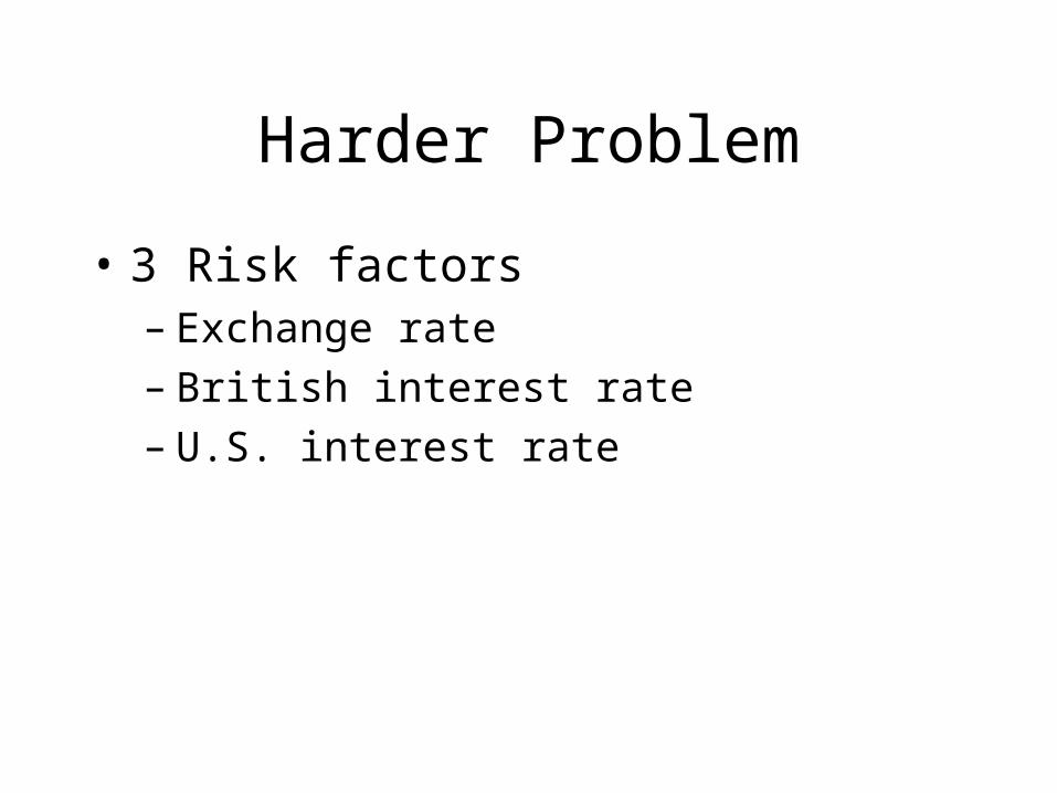
Harder Problem

• 3 Risk factors– Exchange rate– British interest rate– U.S. interest rate

3 Risk Factors1 day ahead value

)055.0)1)(360/90(1(

$15

)06.0)1)(360/90(1(

10)5355.1)(1(

z

y

BPxval

Daily VaR AssessmentHistorical

• Historical VaR

• Get percentage changes for – $/BP: x– r(BP): y– r($): z

• Generate histograms

• matlab: histbpvar2.m

Daily VaR AssessmentBootstrap

• Historical VaR

• Get percentage changes for – $/BP: x– r(BP): y– r($): z

• Bootstrap from these

• matlab: bbpvar2.m

Bootstrap Question:

• Assume independence?– Bootstrap technique differs– matlab: bbpvar2.m

Risk Factors and Multivariate Problems

• Value = f(x, y, z)

• Assume random process for x, y, and z

• Value(t+1) = f(x(t+1), y(t+1), z(t+1))

New Challenges

• How do x, y, and z impact f()?

• How do x, y, and z move together?– Covariance?

Delta Normal Issues

• Life is more difficult for the pure table based delta normal method

• It is now involves– Assume normal changes in x, y, z– Find linear approximations to f()

• This involves partial derivatives which are often labeled with the Greek letter “delta”

• This is where “delta normal” comes from

• We will not cover this

Monte-carlo Method

• Don’t need approximations for f()

• Still need to know properties of x, y, z– Assume joint normal– Need covariance matrix

• ie var(x), var(y), var(z) and

• cov(x,y), cov(x,z), cov(y,z)

Value at Risk: Methods

• Methods– Historical– Delta Normal– Monte-carlo– Bootstrap