VaR and Ruin Probability - ccirm.org · VaR and Ruin probability as risk measures I VaR is a risk measure of S(t) for ﬁxed t. I In ruin theory literature, one usually concerns with

IntroductionExamples: Compound Binomial Risk Model

Brownian motion risk processVaR and Finite Time Ruin probability

VaR and Ruin Probability

Jiandong Ren

University of Western Ontario, London, Ontario, Canada

2011 China International Conference on Insurance and RiskManagement

CICIRM 2011 VaR and Ruin Probability



Introduction–VaR:

Consider an insurance risk setting:I Let {S(t)}t≥0 denote the aggregate operating losses of a

company during time (0, t ].I In VaR literature, one usually concerns the random

variable S(t) for fixed time t . The value at risk at level α isdefined as VaRα(S(t)) = inf{l ,P(S(t) > l) < 1 − α} =inf{l ,FS(t)(l) ≥ α}.

I The probability level α may assume values 0.90, 0.95, or0.99 etc. For example, if a company’s capital level isVaR0.9(S(1)), then there is 90% chance the company willbe able to cover its possible operating losses next timeperiod.




VaR

I VaR is intended to be a risk measure of financial distressover a short period of time. (Pan and Duffie, 1997)

I In finance, the time horizon is usually a number of days. Forexample, the Bank for International Settlements (BIS) set pto 99% and t to ten days for purposes of measuring theadequacy of bank capital. Many firms use an overnight VaRfor internal purposes.

I In insurance, Solvency II requires a 99.5% one year VaR.I Notice that the time horizon in the insurance setting is much

larger than that used in a bank setting, perhaps becauseinsurance transactions are much less frequent than bankingtransactions.




Criticism of VaR

I VaR ignores what happens in the tails. It specifically cutsthem off. A 99% VaR calculation does not evaluate whathappens in the last 1%. (Einhorn 2008)

I By ignoring the tails, VaR creates an incentive to takeexcessive but remote risks. (Einhorn 2008)




Criticism of VaR–Example

I Consider underwriting two potential (annual) losses X andY , where X takes value 1000 with p = 0.001 and zerootherwise; Y takes value 10000 with p = 0.0001 and zerootherwise. An insurer can charge a premium 2 for risk Xand 10 for risk Y .

I The annual aggregate operating loss random variables inthe two situations are S1(1) = X − 2 and S2(1) = Y − 10.

I VaR0.99(S1(1)) = −2 and VaR0.99(S2(1)) = −10. That is,you don’t need any capital to support underwriting the risk.

I A firm has the incentive to take risk Y for extra profit ifcapital requirement is determined by VaR – remote risk isignored by VaR.




Criticism of VaR–Example

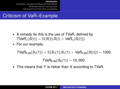
I A remedy for this is the use of TVaR, defined byTVaRα(S(t)) = E(S(t)|S(t) > VaRα(S(t))).

I For our example,

TVaR0.99(S1(1)) = E(S1(1)|S1(1) > VaR0.99(S(t))) = 1000,

TVaR0.99(S2(1)) = 10,000.

I This means that Y is riskier than X according to TVaR.




Criticism of TVaR–Example

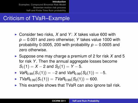
I Consider two risks, X and Y : X takes value 600 withp = 0.001 and zero otherwise; Y takes value 1000 withprobability 0.0005, 200 with probability p = 0.0005 andzero otherwise.

I Suppose one may charge a premium of 2 for risk X and 5for risk Y . Then the annual aggregate losses becomeS1(1) = X − 2 and S2(1) = Y − 5.

I VaR0.99(S1(1)) = −2 and VaR0.99(S2(1)) = −5.I TVaR0.99(S1(1)) = TVaR0.99(S2(1)) = 600.I This example shows that TVaR can also ignore tail risk.




Introduction–Ruin probability

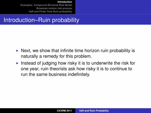
I Next, we show that infinite time horizon ruin probability isnaturally a remedy for this problem.

I Instead of judging how risky it is to underwrite the risk forone year, ruin theorists ask how risky it is to continue torun the same business indefinitely.




Binomial Risk Model

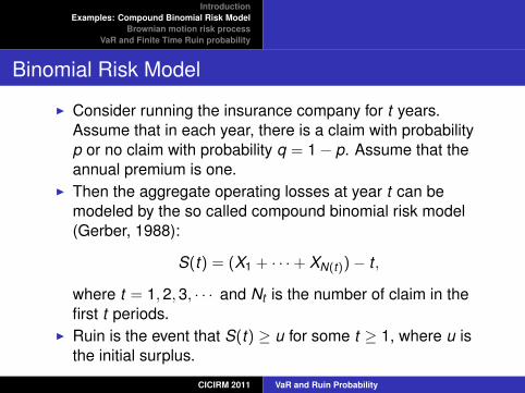
I Consider running the insurance company for t years.Assume that in each year, there is a claim with probabilityp or no claim with probability q = 1 − p. Assume that theannual premium is one.

I Then the aggregate operating losses at year t can bemodeled by the so called compound binomial risk model(Gerber, 1988):

S(t) = (X1 + · · ·+ XN(t))− t ,

where t = 1,2,3, · · · and Nt is the number of claim in thefirst t periods.

I Ruin is the event that S(t) ≥ u for some t ≥ 1, where u isthe initial surplus.




Example 1

We consider two casesI case (1): (denoted by S1(t)), p = 0.001 and the claim sizes

Xi , i = 1,2, · · · be fixed value 600.I case (2): (denoted by S2(t)), p = 0.002 and the claim sizes

Xi , i = 1,2, · · · be fixed value 300.I VaR0.99(S1(1)) = VaR0.99(S2(1)) = −1.I Ruin probability ψ1(u) = P(supt≥1 S1(t) ≥ u), where u is

the initial surplus.




Example 1

I Gerber (1988) showed that ψ1(0) = pE(X ) = 0.6 andψ1(u) = qψ1(u + 1) + p, for 1 < u < 600 andψ1(u) = qψ1(u + 1) + pψ1(u + 1 − 600), for u ≥ 600.

I ψ2(u) can be calculated similarly.I Ruin probabilities as a function of initial surplus in plotted

in figure 1.




Example 1

0 500 1000 1500 2000 2500 30000

0.1

0.2

0.3

0.4

0.5

0.6

0.7

Initial Capital

Rui

n P

roba

bilit

y

p=0.001,x=600p=0.002,x=300

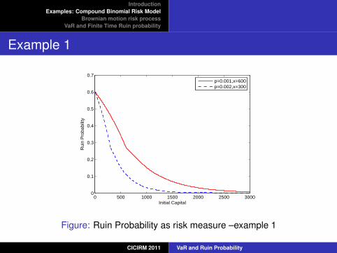
Figure: Ruin Probability as risk measure –example 1




I This figure shows that, when using ruin probability as therisk measure

I {S1(t)}t≥0 is riskier than {S2(t)}t≥0I If one requires that the ultimate ruin probability to be less

than certain level, say 0.1, then the required initial capitalcan be readily determined from the graph.




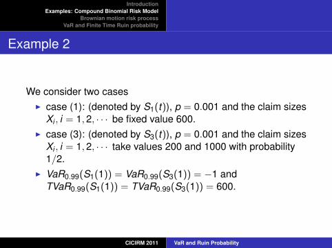
Example 2

We consider two casesI case (1): (denoted by S1(t)), p = 0.001 and the claim sizes

Xi , i = 1,2, · · · be fixed value 600.I case (3): (denoted by S3(t)), p = 0.001 and the claim sizes

Xi , i = 1,2, · · · take values 200 and 1000 with probability1/2.

I VaR0.99(S1(1)) = VaR0.99(S3(1)) = −1 andTVaR0.99(S1(1)) = TVaR0.99(S3(1)) = 600.




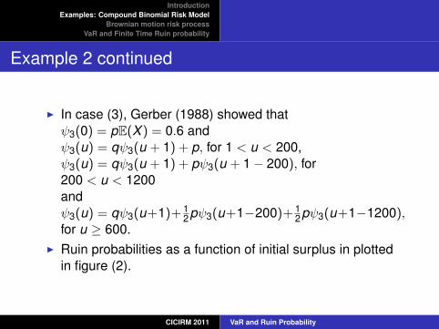
Example 2 continued

I In case (3), Gerber (1988) showed thatψ3(0) = pE(X ) = 0.6 andψ3(u) = qψ3(u + 1) + p, for 1 < u < 200,ψ3(u) = qψ3(u + 1) + pψ3(u + 1 − 200), for200 < u < 1200andψ3(u) = qψ3(u+1)+ 1

2pψ3(u+1−200)+ 12pψ3(u+1−1200),

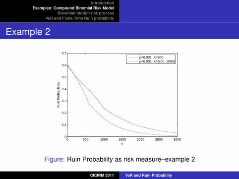
for u ≥ 600.I Ruin probabilities as a function of initial surplus in plotted

in figure (2).




Example 2

0 500 1000 1500 2000 2500 30000

0.1

0.2

0.3

0.4

0.5

0.6

0.7

u

Rui

n P

roba

bilit

ies

p=0.001, X=600p=0.001, X=[200, 1000]

Figure: Ruin Probability as risk measure–example 2




VaR and Ruin probability as risk measures

I VaR is a risk measure of S(t) for fixed t .I In ruin theory literature, one usually concerns with the

random variable M(∞) = sup{S(x),0 ≤ x}.I the infinite time horizon ruin probability is defined byψ(u) = P(M(∞) > u). That is, ruin probability is a riskmeasure of M(∞)

I These two measures provide different information aboutthe risk in concern.

I Instead of judging how risky it is to bet on one trial offlipping a coin, ruin theorists ask how risky it is to continuebetting on a lot of trials.




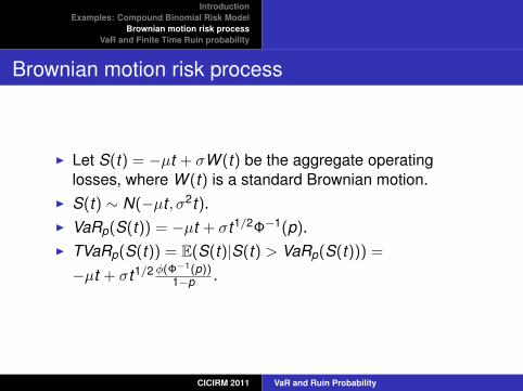
Brownian motion risk process

I Let S(t) = −µt + σW (t) be the aggregate operatinglosses, where W (t) is a standard Brownian motion.

I S(t) ∼ N(−µt , σ2t).I VaRp(S(t)) = −µt + σt1/2Φ−1(p).I TVaRp(S(t)) = E(S(t)|S(t) > VaRp(S(t))) =

−µt + σt1/2 ϕ(Φ−1(p))1−p .




Brownian motion risk process

I Infinite time horizon ruin probability concernsM(∞) = supt≥0{S(t)}.

I FM(∞)(y) = 1 − e2µy/σ2, for µ > 0.

I We next illustrate how VaR and ruin probability differ in thiscase.




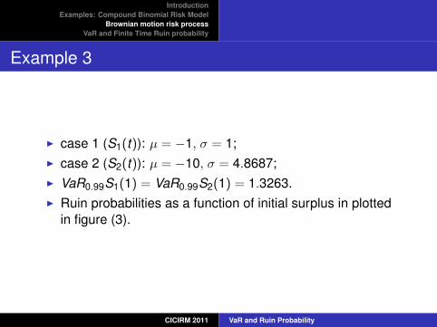
Example 3

I case 1 (S1(t)): µ = −1, σ = 1;I case 2 (S2(t)): µ = −10, σ = 4.8687;I VaR0.99S1(1) = VaR0.99S2(1) = 1.3263.I Ruin probabilities as a function of initial surplus in plotted

in figure (3).




Example 3

1 2 3 4 5 6 7 8 9 100

0.05

0.1

0.15

0.2

0.25

0.3

0.35

0.4

0.45

Initial Capital

Rui

n P

roba

bilit

ies

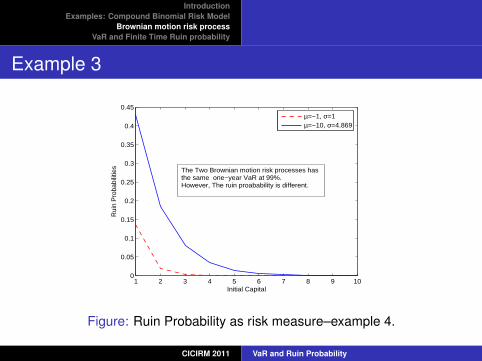
µ=−1, σ=1µ=−10, σ=4.869

The Two Brownian motion risk processes has the same one−year VaR at 99%.However, The ruin proabability is different.

Figure: Ruin Probability as risk measure–example 4.




Conclusion of the examples

I VaR and TVaR consider the short term effect of a risk.I By looking at the long term effect of the risk, ruin probability

supplement VaR and TVaR as a informative risk measure.




VaR and Finite Time Ruin probability

I Define M(t) = sup{S(x),0 ≤ x ≤ t}. for some fixed t .I The ruin probability with time horizon t is defined byψ(u, t) = P(M(t) > u), where u is the insurer’s initialcapital level.

I The surplus level to ensure that the t year ruin probabilityis less than a small probability 1 − α isRα(S(t)) = inf{l ,FM(t)(l) ≥ α} = VaRα(M(t)).

I Obviously, Rα(S(t)) ≥ VaRα(S(t))




Analysis of the time horizon

I Is the one–year horizon used by Solvency II for insurancecompany too long?

I What is chance of something very bad occurs during (0, t)?





I This question has been analyzed by Boukoudh et al.(2004), in which the authors argue that, with reasonableparameters, the interim risk (M(t)) could exceed S(t) by40%.





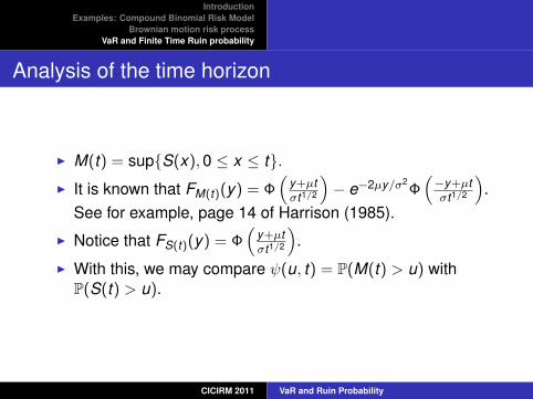
I M(t) = sup{S(x),0 ≤ x ≤ t}.I It is known that FM(t)(y) = Φ

(y+µtσt1/2

)− e−2µy/σ2

Φ(−y+µtσt1/2

).

See for example, page 14 of Harrison (1985).

I Notice that FS(t)(y) = Φ(

y+µtσt1/2

).

I With this, we may compare ψ(u, t) = P(M(t) > u) withP(S(t) > u).




Analysis of the time horizon–an approximation

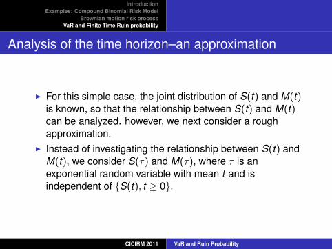
I For this simple case, the joint distribution of S(t) and M(t)is known, so that the relationship between S(t) and M(t)can be analyzed. however, we next consider a roughapproximation.

I Instead of investigating the relationship between S(t) andM(t), we consider S(τ) and M(τ), where τ is anexponential random variable with mean t and isindependent of {S(t), t ≥ 0}.




Analysis of the time horizon–an approximation

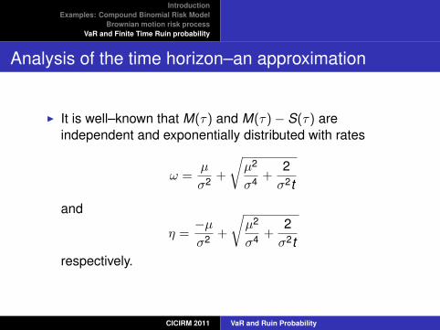
I It is well–known that M(τ) and M(τ)− S(τ) areindependent and exponentially distributed with rates

ω =µ

σ2 +

√µ2

σ4 +2σ2t

and

η =−µσ2 +

√µ2

σ4 +2σ2t

respectively.





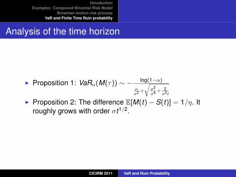
I Proposition 1: VaRα(M(τ)) ∼ − log(1−α)

µ

σ2 +

√µ2

σ4 +2

σ2t

I Proposition 2: The difference E[M(t)− S(t)] = 1/η. Itroughly grows with order σt1/2.




Conclusion

By looking at the long term effect of the risk, ruin probabilitysupplement VaR and TVaR as a informative risk measure.




Conclusion

Thank you!


Documents

VaR and Ruin Probability - ccirm.org · VaR and Ruin probability as risk measures I VaR is a risk measure of S(t) for ﬁxed t. I In ruin theory literature, one usually concerns with