Embed Size (px)
Citation preview
VAPOR PRESSURE DATA ANALYSIS AND STATISTICS
ECBC-TR-1422
Ann Brozena
RESEARCH AND TECHNOLOGY DIRECTORATE
Charles E. Davidson Avishai Ben-David
SCIENCE AND TECHNOLOGY CORPORATION, INC. Belcamp, MD 21017-1427
Bryan Schindler
LEIDOS, INC. Gunpowder, MD 21010-0068
David E. Tevault
JOINT RESEARCH AND DEVELOPMENT, INC. Belcamp, MD 21017-1552
December 2016
Approved for public release; distribution unlimited.

Disclaimer
The findings in this report are not to be construed as an official Department of the Army position unless so designated by other authorizing documents.
REPORT DOCUMENTATION PAGE Form Approved
OMB No. 0704-0188 Public reporting burden for this collection of information is estimated to average 1 h per response, including the time for reviewing instructions, searching existing data sources, gathering and maintaining the data needed, and completing and reviewing this collection of information. Send comments regarding this burden estimate or any other aspect of this collection of information, including suggestions for reducing this burden to Department of Defense, Washington Headquarters Services, Directorate for Information Operations and Reports (0704-0188), 1215 Jefferson Davis Highway, Suite 1204, Arlington, VA 22202-4302. Respondents should be aware that notwithstanding any other provision of law, no person shall be subject to any penalty for failing to comply with a collection of information if it does not display a currently valid OMB control number. PLEASE DO NOT RETURN YOUR FORM TO THE ABOVE ADDRESS.
1. REPORT DATE
XX-12-2016 2. REPORT TYPE
Final 3. DATES COVERED (From - To)
Nov 2015 – Apr 2016
4. TITLE
Vapor Pressure Data Analysis and Statistics 5a. CONTRACT NUMBER
5b. GRANT NUMBER
5c. PROGRAM ELEMENT NUMBER
6. AUTHORS
Brozena, Ann (ECBC); Davidson, Charles E.; Ben-David, Avishai (STC);
Schindler, Bryan (Leidos); and Tevault, David E. (JRAD)
5d. PROJECT NUMBER: Chemical and Biological
Defense Technology Base Program 5e. TASK NUMBER
5f. WORK UNIT NUMBER
7. PERFORMING ORGANIZATION NAMES AND ADDRESSES
Director, ECBC, ATTN: RDCB-DRC-P, APG, MD 21010-5424
Science and Technology Corporation, Inc. (STC), 111 Bata Boulevard,
Suite C, Belcamp, MD 21017-1427
Leidos, Inc., P.O. Box 68, Gunpowder, MD 21010-0068
Joint Research and Development, Inc. (JRAD), 4694 Millennium Drive,
Suite 105, Belcamp, MD 21017-1552
8. PERFORMING ORGANIZATION REPORT NUMBER
ECBC-TR-1422
9. SPONSORING / MONITORING AGENCY NAME(S) AND ADDRESS(ES)
Defense Threat Reduction Agency, 8725 John J. Kingman Road, MSC 6201,
Fort Belvoir, VA 22060-6201
10. SPONSOR/MONITOR’S ACRONYM(S)
DTRA 11. SPONSOR/MONITOR’S REPORT NUMBER(S)
12. DISTRIBUTION/AVAILABILITY STATEMENT
Approved for public release; distribution unlimited.
13. SUPPLEMENTARY NOTES
14. ABSTRACT:
This report compares several methods for expressing vapor pressure as a function of temperature (also referred to as
correlation in the traditional literature) using the Antoine equation and discusses statistical analyses of the resulting
correlations. Vapor pressure varies nonlinearly with temperature and is an important property of materials for applications
ranging from estimates of their behavior in the environment to design of test equipment. Vapor pressure and temperature
measurements over wide dynamic ranges are difficult to obtain, and prediction of vapor pressure based on limited data may be
required in certain cases, necessitating reliable relationships between pressure and temperature. While the integrated form of
the Clausius–Clapeyron equation has sound theoretical basis for correlating pressure and temperature, assumptions required for
the temperature dependence of enthalpy may not be valid, particularly over wide temperature ranges. To correct for those
approximations, a modified correlation equation may be implemented to enable accurate extrapolation. One variation of the
Clausius–Clapeyron equation is the Antoine equation, which incorporates a third fit parameter to more accurately describe the
nonlinearity of vapor pressure data. The current results support the use of the procedure proposed by Penski and Latour as the
best method for correlating vapor pressure data.
15. SUBJECT TERMS
Vapor pressure Antoine equation Statistical analysis Clausius–Clapeyron equation
Standard deviation Volatility Enthalpy of volatilization Entropy of volatilization
16. SECURITY CLASSIFICATION OF:
17. LIMITATION OF ABSTRACT
UU
18. NUMBER OF PAGES
42
19a. NAME OF RESPONSIBLE PERSON
Renu B. Rastogi
a. REPORT
U
b. ABSTRACT
U
c. THIS PAGE
U
19b. TELEPHONE NUMBER (include area code)
(410) 436-7545 Standard Form 298 (Rev. 8-98)
Prescribed by ANSI Std. Z39.18

ii
Blank
iii
PREFACE
The work described in this report was authorized under the Chemical and
Biological Defense Technology Base Program. The work was started in November 2015 and
completed in April 2016.
The use of either trade or manufacturers’ names in this report does not constitute
an official endorsement of any commercial products. This report may not be cited for purposes of
advertisement.
This report has been approved for public release.
Acknowledgments
The authors would like to salute Mr. Elwin Penski (former ECBC employee) for
his pioneering work that inspired this report. We also acknowledge technical guidance provided
by Dr. John Mahle (ECBC). We also extend our gratitude to Ms. Janett Stein (ECBC library) for
technical assistance.

iv
Blank
v
CONTENTS
1. INTRODUCTION ...................................................................................................1
2. VAPOR PRESSURE CORRELATIONS ................................................................1
3. FITTING METHODS ..............................................................................................4
4. STATISTICAL ANALYSIS ...................................................................................7
5. RESULTS AND DISCUSSION ..............................................................................9
5.1 1-Hexadecanol .................................................................................................10
5.2 1-Tetradecanol .................................................................................................11
5.3 DEM .................................................................................................................13
5.4 VX ....................................................................................................................14
5.5 RVX .................................................................................................................15
5.6 TDG .................................................................................................................16
5.7 N,N′-Diisopropylcarbodiimide (DICDI) ..........................................................17
6. CONCLUSIONS....................................................................................................19
LITERATURE CITED ..........................................................................................21
ACRONYMS AND ABBREVIATIONS ..............................................................23
APPENDIX: SCREENSHOTS OF MICROSOFT EXCEL TEMPLATE ............25
vi
FIGURE
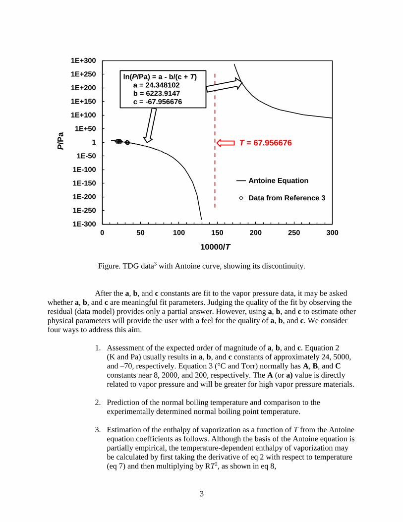
TDG data3 with Antoine curve, showing its discontinuity ..................................................3
TABLES
1. 1-Hexadecanol Vapor Pressure Data from Kemme and Kreps11 .......................................10
2. Antoine Constants (Equation 3), Standard Deviations, and S for 1-Hexadecanol .............10
3. Vapor Pressures (Torr, Equation 3) Calculated at Selected Temperatures
for 1-Hexadecanol Using Constants Listed in Table 2 ......................................................11
4. 1-Tetradecanol Vapor Pressure Data from Kemme and Kreps11 .......................................11
5. Antoine Constants (Equation 3), Standard Deviations, and S for 1-Tetradecanol .............12
6. Vapor Pressures (Torr, Equation 3) Calculated at Selected Temperatures
for 1-Tetradecanol Using Constants Listed in Table 5 ......................................................13
7. Antoine Constants (Equation 3), Standard Deviations, and S for DEM ............................13
8. Vapor Pressures (Torr, Equation 3) Calculated at Selected Temperatures
for DEM Using Constants Listed in Table 7 .....................................................................14
9. Antoine Constants (Equation 2), Standard Deviations, and S for VX ...............................15
10. Vapor Pressures (Pascal, Equation 2) Calculated at Selected Temperatures
for VX Using Constants Listed in Table 9 and Differences from Values
Calculated Using the Penski Method (Excel Software) .....................................................15
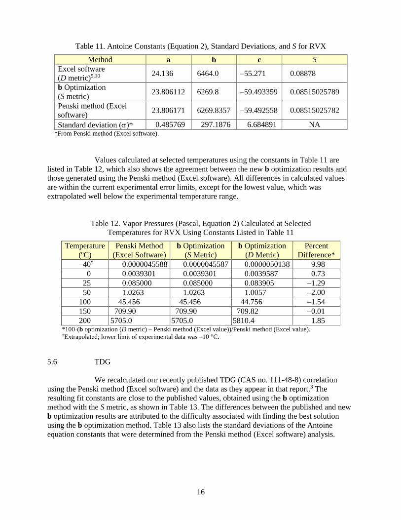
11. Antoine Constants (Equation 2), Standard Deviations, and S for RVX ............................16
12. Vapor Pressures (Pascal, Equation 2) Calculated at Selected Temperatures
for RVX Using Constants Listed in Table 11 ....................................................................16
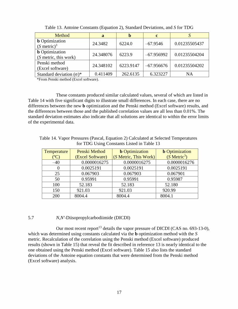
13. Antoine Constants (Equation 2), Standard Deviations, and S for TDG .............................17
14. Vapor Pressures (Pascal, Equation 2) Calculated at Selected Temperatures
for TDG Using Constants Listed in Table 13 ....................................................................17
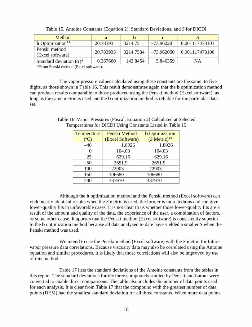
15. Antoine Constants (Equation 2), Standard Deviations, and S for DICDI ..........................18
16. Vapor Pressures (Pascal, Equation 2) Calculated at Selected Temperatures
for DICDI Using Constants Listed in Table 15 .................................................................18
17. Standard Deviations of Antoine Constants for Compounds and Data in This Report.......19
Note: Throughout this report, Antoine and Clausius–Clapeyron equation correlation constants are shown
in bold for clarity.
1
VAPOR PRESSURE DATA ANALYSIS AND STATISTICS
1. INTRODUCTION
Knowledge of the vapor pressure of materials as a function of temperature is
important for a number of reasons, including prediction of their behavior when released into the
environment or laboratory, design of test apparatus for developmental test equipment, and
determination of route(s) of entry for toxicological assessments. Vapor pressure-versus-
temperature relationships can also be used to calculate the normal boiling point, temperature-
dependent enthalpy of volatilization (vaporization for liquids and sublimation for solids),
volatility, and entropy of volatilization. Vapor pressure can be reported several different ways,
including tables of experimental temperature and pressure pairs, smoothed pressure values
calculated at selected temperatures, or correlated equations expressing vapor pressure as a
function of temperature. Vapor pressure data are plotted by convention on a scale of logarithm of
pressure versus reciprocal temperature to give a straight or nearly straight line plot. When data
are plotted over wide ranges, the nonlinearity of the data becomes obvious, requiring a more
complicated mathematical relationship (also commonly referred to as correlation in the
literature) to accurately describe the data and enable interpolation and extrapolation.
The purposes of this report are to compare several different methods for
correlating vapor pressure data using the Antoine equation and to discuss statistical analyses of
the resulting correlations.
2. VAPOR PRESSURE CORRELATIONS
Many different equations can be used to express vapor pressure as a function of
temperature. This report addresses the two most prevalent in the literature, the Clausius–
Clapeyron and Antoine equations.1
The Clausius–Clapeyron equation has the following form:
ln(𝑃) = 𝐚 −𝐛
𝑇
where P is vapor pressure (Pa), T is absolute temperature (K), and a and b are correlation
constants. The derivation of this equation has a sound thermodynamic basis, but it is based on
several assumptions that are not exact. These are, primarily, that heat of vaporization (the slope
of the vapor pressure curve) does not vary with temperature, and also that the molar volume of
the liquid is negligible compared to that of the vapor. Although the integrated form of the
Clausius–Clapeyron equation is linear on a standard plot (lnP vs 1/T), the assumption of constant
enthalpy of vaporization is not valid over wide temperature ranges. As a result, this equation
only accurately represents data over narrow temperature ranges.
(1)
2
The modified integrated Clausius–Clapeyron and other empirical relations have
been developed to better describe vapor pressure data. One of these modifications is the Antoine
equation (eq 2, for Kelvin and Pascal units; eq 3 for Celsius and Torr units), which is easy to
solve, less cumbersome than higher-term equations, takes into account the variation in heat of
vaporization with temperature, and accurately describes data over broad experimental ranges,
thereby enabling interpolation and limited extrapolation of the data.
ln(𝑃) = 𝐚 −𝐛
(𝐜 + 𝑇)
where P is vapor pressure (Pa); T is absolute temperature (K); a, b, and c are correlation
constants; and ln denotes the natural logarithm. The c value is usually negative, reflecting the
negative curvature of the vapor pressure plot and decreasing enthalpy of vaporization as
temperature increases.
log(𝑝) = 𝐀 −𝐁
(𝐂 + 𝑡)
where p is vapor pressure (Torr); t is Celsius temperature; A, B, and C are correlation constants;
and log denotes logarithm in base 10. For these units, a C value less than 273.15 reflects the
slight negative curvature typically observed for vapor pressure data over a large temperature
range.
Although other combinations of units are found in the literature for the Antoine
equation, the current discussion is limited to the two listed above, which can be interconverted to
express pressure and temperature as Pascal and Kelvin (eq 2) or Torr and Celsius (eq 3) using
eqs 4–6. The units used here conform with those used in the original reports.
a = A ln(10) + ln(101325/760) (4)
b = B ln(10) (5)
c = C – 273.15 (6)
The advantages and disadvantages of the Antoine equation have been summarized
by Penski.2 An additional disadvantage of the Antoine equation is that the predicted pressure is
incorrect at temperatures far below the experimental temperature limit; the calculated vapor
pressure becomes undefined when the denominator approaches zero, such as when the absolute
value of the (negative) c constant is equal to the experimental temperature. This anomaly makes
it inappropriate to extrapolate significantly below the low-temperature limit of the data. An
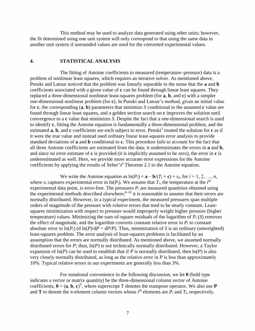
example of this effect is illustrated by the Antoine equation for thiodiglycol (TDG)3 in the figure.
That said, since absolute values of c are usually less than 100, this deficiency of the Antoine
model is often of academic interest only. A quantitative assessment of the extrapolation accuracy
to lower temperatures has not been fully investigated.
(2)
(3)
3
Figure. TDG data3 with Antoine curve, showing its discontinuity.
After the a, b, and c constants are fit to the vapor pressure data, it may be asked
whether a, b, and c are meaningful fit parameters. Judging the quality of the fit by observing the
residual (data model) provides only a partial answer. However, using a, b, and c to estimate other
physical parameters will provide the user with a feel for the quality of a, b, and c. We consider
four ways to address this aim.
1. Assessment of the expected order of magnitude of a, b, and c. Equation 2
(K and Pa) usually results in a, b, and c constants of approximately 24, 5000,
and –70, respectively. Equation 3 (°C and Torr) normally has A, B, and C
constants near 8, 2000, and 200, respectively. The A (or a) value is directly
related to vapor pressure and will be greater for high vapor pressure materials.
2. Prediction of the normal boiling temperature and comparison to the
experimentally determined normal boiling point temperature.
3. Estimation of the enthalpy of vaporization as a function of T from the Antoine
equation coefficients as follows. Although the basis of the Antoine equation is
partially empirical, the temperature-dependent enthalpy of vaporization may
be calculated by first taking the derivative of eq 2 with respect to temperature
(eq 7) and then multiplying by RT2, as shown in eq 8,
1E-300
1E-250
1E-200
1E-150
1E-100
1E-50
1
1E+50
1E+100
1E+150
1E+200
1E+250
1E+300
0 50 100 150 200 250 300
P/P
a
10000/T
Antoine Equation
Data from Reference 3
ln(P/Pa) = a - b/(c + T) a = 24.348102b = 6223.9147c = -67.956676
T = 67.956676
4
d ln (𝑃)
d𝑇=
𝐛
(𝐜 + 𝑇)2
∆𝐻vap =d ln (𝑃)
d𝑇 R𝑇2 = 𝐛R
𝑇2
(𝐜 + 𝑇)2
where Hvap is enthalpy of vaporization (or enthalpy of sublimation for
solids). Over narrow temperature ranges, c is often neglected, eq 8 reduces to
eq 9, and the calculated enthalpy of vaporization does not depend on
temperature.
Hvap = bR (9)
4. Calculation of the entropy of vaporization, which is defined as the enthalpy of
vaporization at the normal boiling point divided by the normal boiling point
temperature. Trouton’s rule states that this value should be approximately
89 J/mol-K, although deviations to higher values due to hydrogen bonding
may be expected.
Using the model fit parameters to identify potentially flawed experimental data
can be instructive. An example is provided by TDG; its vapor pressure was first reported by
Bauer and Burschkies4 in 1935 without a correlation equation. The a and b correlation constants
for the Clausius–Clapeyron equation based on their data are unusually low, the extrapolated
normal boiling point of greater than 1300 K is unreasonably high, and the calculated enthalpy of
vaporization of less than 20 kJ/mole is extraordinarily low, suggesting problems with the data.
New data published in 2014 by Brozena et al.3 suggested a more realistic normal boiling point
(553 K) and standard enthalpy of vaporization (86.8 kJ/mole) and are in good agreement with
recent manufacturers’ data. In addition, values for the constants and derived thermodynamic
properties are in the expected ranges. Numerical analysis would have suggested that there were
flaws in the original data prior to its publication.
3. FITTING METHODS
Our process for correlating experimental vapor pressure data to either the Antoine
or Clausius–Clapeyron equation has evolved over time with updates, as required, based on the
computer technology available and our understanding of the options for fit optimization. Several
different but related methods are addressed in this report. All of these methods are based on
least-squares solutions; the Clausius–Clapeyron equation is linear when plotted on a standard
vapor pressure plot of ln(P) versus T–1, whereas the Antoine equation is nonlinear with negative
curvature on such a plot.
Unless otherwise stated, the metric used to optimize the fits described in this
report is least-squares error applied to the logarithm of pressure, which is the sum of the squares
(7)
(8)
5
of the differences between the logarithms of experimental and calculated values, referred to by
Penski2 and in this report as S:
𝑆 = ∑ (𝑌𝑖 − 𝐚 − 𝐛𝑋𝑖)2
𝑖=1,𝑛 (10)
where n is the number of data points, Yi is the natural logarithm of the ith experimental vapor
pressure value, and Xi is the negative reciprocal of the sum of the c constant and the ith
experimental temperature value. For O-ethyl S-(2-diisopropylaminoethyl) methyl
phosphonothiolate and O-isobutyl-S-[2(diethylamino)ethyl] methylphosphonothiolate (VX and
RVX, respectively), the sum of the absolute values of the percent differences between the
experimental and calculated values was used as the metric.
In 1971, Penski and Latour developed and described in detail5 a Fortran program
to find values for A, B, and C that minimize S, which is a nonlinear regression problem and
therefore requires an iterative solution procedure. The problem is nonlinear because of the C
coefficient; A and B appear linear if the value of C is known. Penski and Latour’s method takes
advantage of this conditional linearity by performing a one-dimensional golden section search to
find the optimal value of C given a reasonable starting value. At each iteration, the optimal A
and B values given the current value of C are easily found as a solution to a linear least-squares
problem. This method was updated in 1989 by Dr. Kenneth Collins (U.S. Army Edgewood
Chemical Biological Center [ECBC]) to a Basic program, enabling the fit to be performed using
a desktop computer.2
In 1992, Penski updated his method2 to address a number of deficiencies,
including the lack of statistical analysis of the least-squares fitting. This update included
equations to estimate the standard errors of the A and B Antoine coefficients; however, Penski
treated the solution value of C as if it were exact. In reality, because C is determined from the
data, it is also subject to error; and the error in C also must be propagated to A and B. As a result
of this oversight, the standard errors of A and B as estimated by Penski’s equations are too small.
For example, Penski’s A and B values for diethyl malonate (DEM) in Appendix I of reference 2
are 0.020955 and 3.200, respectively, compared to our values, 0.0573171 and 33.9768. In the
following discussion, we correct the statistical analysis of the Antoine equation and provide more
accurate equations for estimating the scatter in the data used to determine the Antoine fit, using
standard nonlinear regression theory.6 Penski also pointed out that the correlations presented in
1971 were determined using low-precision calculations, and that higher-precision calculations
produced better fits to the experimental data, as determined by the S values.
In the late 1990s, we recognized the need to update our vapor pressure correlation
capabilities to something more flexible with wider availability than Penski’s Fortran program. A
Microsoft Excel spreadsheet using the Solver program was developed in-house and appeared to
have the desired capability. This approach, which was also based on a least-squares optimization
scheme, relies on minimizing S (eq 10). One drawback of this method was the requirement to
provide reasonable starting estimates of the correlation constants in order for the Solver program
to find the optimum solution.
Several modifications of the Excel spreadsheet have been explored. In an attempt
to optimize the correlation of data sets including outliers, an alternate metric was employed,
6
minimizing the sum of the absolute values of the percent differences between the experimental
and calculated values, D, a metric that appears to minimize the influence of experimental outliers
on the overall fit.7
Another modification of the basic Excel Solver procedure, identified herein as the
“b optimization method”, is performed by varying the b constant and allowing Solver to
determine values of a and c that minimize S. This method of deriving Antoine equation
coefficients from experimental data by optimization of the b constant is tedious in that it requires
manual variation of b for each iteration. In some instances, the coefficients produced by this
method were found to depend on the starting values selected for the a and c constants, thereby
yielding unoptimized “solutions”. These unreliable solutions can be identified most easily by
graphing S versus b in real time to determine which points do not lie on a smooth curve and,
therefore, should be disregarded. This unpredictable reliability, especially the dependence of the
solution on the initial values of the a and c constants, caused us to search for an alternative
method that combined the robustness of Penski’s original and updated methods with the
availability and flexibility of Excel software.
Recently we adapted Penski’s method to make it compatible with Excel software
using Solver and the S metric. This method has the advantage of not requiring operator
intervention to arrive at the optimum solution. Although we found a few examples in which
Penski’s method could not optimize the correlation due to the selection of the c constant starting
value, those cases appear to be rare and easily identifiable.
The Penski method (using Excel software) is described as follows:
Enter the total number of data points (n) representing the experimental data
pairs (vapor pressure and temperature) into separate columns in the Excel (or
similar) worksheet.
Using eqs 8 and 9 in Penski and Latour’s report,5 calculate Xi, Yi, Xi2, Yi
2, XiYi,
and their sums.
Calculate the Antoine b constant using eq 11 in reference 5 with the total
number of data points and sums of Xi, Yi, Xi2, and XiYi values; where Xi equals
–1/(c + T), Yi equals ln(Pi), and S equals the sum of the squares of the
differences of the natural logarithms of experimental and correlated vapor
pressure values, as described in Penski and Latour’s report.5
Calculate the Antoine a constant using eq 10 in reference 5 with the Antoine
b constant from the previous step, the total number of data points, and the
sums of the Xi and Yi values.
Compute S according to eq 10 in this report using the total number of data
points; the sums of Xi, Yi, Xi2, Yi
2, and XiYi values; and the Antoine a and b
constants from above.
Using the Excel Solver program, find the value of c that minimizes S. This
step also generates solution values for a and b.
7
This method may be used to analyze data generated using other units; however,
the fit determined using one unit system will only correspond to that using the same data in
another unit system if unrounded values are used for the converted experimental values.
4. STATISTICAL ANALYSIS
The fitting of Antoine coefficients to measured (temperature–pressure) data is a
problem of nonlinear least squares, which requires an iterative solver. As mentioned above,
Penski and Latour noticed that the problem was linearly separable in the sense that the a and b
coefficients associated with a given value of c can be found through linear least squares. They
replaced a three-dimensional nonlinear least-squares problem (for a, b, and c) with a simpler
one-dimensional nonlinear problem (for c). In Penski and Latour’s method, given an initial value
for c, the corresponding (a, b) parameters that minimize S conditional to the assumed c value are
found through linear least squares, and a golden section search on c improves the solution until
convergence to a c value that minimizes S. Despite the fact that a one-dimensional search is used
to identify c, fitting the Antoine equation is fundamentally a three-dimensional problem, and the
estimated a, b, and c coefficients are each subject to error. Penski2 treated the solution for c as if
it were the true value and instead used ordinary linear least-squares error analysis to provide
standard deviations of a and b conditional to c. This procedure fails to account for the fact that
all three Antoine coefficients are estimated from the data; it underestimates the errors in a and b,
and since no error estimate of c is provided (it is implicitly assumed to be zero), the error in c is
underestimated as well. Here, we provide more accurate error expressions for the Antoine
coefficients by applying the results of Seber’s6 Theorem 2.1 to the Antoine equation.
We write the Antoine equation as ln(Pi) = a – b/(Ti + c) + εi, for i = 1, 2, …, n,
where εi captures experimental error in ln(Pi). We assume that Ti, the temperature at the ith
experimental data point, is error-free. The pressures Pi are measured quantities obtained using
the experimental methods described elsewhere;8–10 it is reasonable to assume that their errors are
normally distributed. However, in a typical experiment, the measured pressures span multiple
orders of magnitude of the pressure with relative errors that tend to be nearly constant. Least-
squares minimization with respect to pressure would improperly weight higher pressure (higher
temperature) values. Minimizing the sum-of-square residuals of the logarithm of Pi (S) removes
the effect of magnitude, and the logarithm converts constant relative error in Pi to constant
absolute error in ln(Pi) (d ln(P)/dP = dP/P). Thus, minimization of S is an ordinary (unweighted)
least-squares problem. The error analysis of least-squares problems is facilitated by an
assumption that the errors are normally distributed. As mentioned above, we assumed normally
distributed errors for P; thus, ln(P) is not technically normally distributed. However, a Taylor
expansion of ln(P) can be used to establish that if P is normally distributed, then ln(P) is also
very closely normally distributed, as long as the relative error in P is less than approximately
10%. Typical relative errors in our experiments are generally less than 3%.
For notational convenience in the following discussion, we let θ (bold type
indicates a vector or matrix quantity) be the three-dimensional column vector of Antoine
coefficients, θ = (a, b, c)T, where superscript T denotes the transpose operator. We also use P
and T to denote the n-element column vectors whose ith elements are Pi and Ti, respectively.
8
The error analysis of a nonlinear regression problem hinges on a first-order Taylor
expansion of the model equation around the solution value. As long as the model equation is
sufficiently linear in a region around the true solution, asymptotic results from standard linear
least squares apply. For our purpose, it is most important that the least-squares solution value θ is
normally distributed, unbiased, and has a covariance matrix given by σ2Σ−1, where superscript −1
denotes the matrix inverse, and 2 is the variance of ln(P) around the model fit. The matrix Σ is
given by
)()( lnlnTT θ
PT
θ
P
where Tθ
P
ln is the n-by-3 matrix of first derivatives of the model equation with respect to the
coefficients. The ith row of the first derivative matrix is given by
2)(
11
lnlnlnln
c
b
ccbaθ ii
iii
T
i
TT
PPPP
The first derivative matrix may also be written as
2)(
1lnlnlnln
c
b
c1
caθ TT
PPPPT
b
where 1 is the n-element vector whose elements all equal 1, and all mathematical operations are
understood to be element-by-element (for instance, 1/T would indicate the vector consisting of
reciprocals of the elements of the n-element vector T). The elements of the matrix Σ are given
here explicitly:
n
i
i
n
i
i
n
i
i
n
i
i
n
i
i
n
i
i
n
i
i
n
i
i
TTT
TTT
TTn
1
42
1
3
1
2
1
3
1
2
1
1
1
2
1
1
)()()(
)()()(
)()(
cbcbcb
cbcc
cbc
Σ
Note that the matrix is symmetric and involves only six unique quantities (corresponding to
either the upper or lower triangular portion of the matrix).
Although σ2 may not be known a priori, an estimate is given by )3(ˆ 2 nS ,
where n – 3 is the number of degrees of freedom for n data points minus the three variables, a, b,
and c; therefore, the standard errors of the Antoine coefficients may be estimated by the square
roots of the diagonal elements of 12ˆ
Σ . It should be noted that the covariance matrix 12ˆ
Σ is in
9
general not a diagonal matrix, and that the a, b, and c parameters can be highly correlated. This
is reflective of the fact that if one of the parameter values is changed from the optimum value,
the other two can compensate, reducing the increase in the S value.
We caution the reader that the high correlation of the error in a, b, and c must be
kept in mind because it impacts the calculation of confidence intervals. One common simple
technique that might be tempting to visualize approximate confidence intervals would be to plot
the model curve corresponding to (a ± kσa, b, c), (a, b ± kσb, c), and (a, b, c ± kσc), where k is
some factor intended to achieve a certain quantile of a normal distribution. This corresponds to
visualizing the model when each of the parameters is perturbed in turn (with the two other
parameters remaining at their solution values). This technique should be strongly discouraged
because it ignores the correlation between the parameters (it does not allow for the other
parameters to be modified to compensate for a change in the parameter being perturbed), and
therefore, it will be misleading, showing errors that will be too large. Methods for estimating
approximate confidence intervals for nonlinear regression problems are discussed in detail
elsewhere.6 In general, if the problem is sufficiently linear around the solution value, then
confidence intervals from linear regression theory are appropriate.
The calculations for the standard deviations are summarized as follows:
Calculate
n
i
iT1
2)( c ,
n
i
iT1
3)( c , and
n
i
iT1
4)( c ;
Calculate 2 = S/(n – 3);
Construct the matrix and its inverse and
Calculate standard deviations of a, b, and c Antoine equation constants using
2 and diagonals of inverted matrix, a = (2 –1[1,1])1/2;
b = ( 2 –1[2,2])1/2; and c = ( 2 –1[3,3])1/2, where the notation –1[i,i]
refers to the ith diagonal element of the matrix –1.
5. RESULTS AND DISCUSSION
Two data sets analyzed by Penski and Latour5 and one set by Penski2 were used in
this work to demonstrate how the more recent correlation approaches (the Excel version of
Penski’s method and b optimization) compare to the results obtained using the earlier methods.
Those are discussed here in detail. Four other examples contained in recent publications from our
laboratory were examined using Penski’s method (Excel software) and are compared to the
published results, which were determined using the b optimization method. The published
Antoine constants for VX and RVX were derived using a different metric, as described in
Sections 5.4 and 5.5, respectively.
10
5.1 1-Hexadecanol
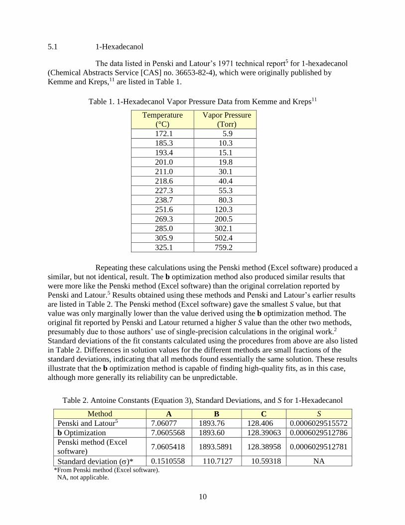
The data listed in Penski and Latour’s 1971 technical report5 for 1-hexadecanol
(Chemical Abstracts Service [CAS] no. 36653-82-4), which were originally published by
Kemme and Kreps,11 are listed in Table 1.
Table 1. 1-Hexadecanol Vapor Pressure Data from Kemme and Kreps11
Temperature
(°C)
Vapor Pressure
(Torr)
172.1 5.9
185.3 10.3
193.4 15.1
201.0 19.8
211.0 30.1
218.6 40.4
227.3 55.3
238.7 80.3
251.6 120.3
269.3 200.5
285.0 302.1
305.9 502.4
325.1 759.2
Repeating these calculations using the Penski method (Excel software) produced a
similar, but not identical, result. The b optimization method also produced similar results that
were more like the Penski method (Excel software) than the original correlation reported by
Penski and Latour.5 Results obtained using these methods and Penski and Latour’s earlier results
are listed in Table 2. The Penski method (Excel software) gave the smallest S value, but that
value was only marginally lower than the value derived using the b optimization method. The
original fit reported by Penski and Latour returned a higher S value than the other two methods,
presumably due to those authors’ use of single-precision calculations in the original work.2
Standard deviations of the fit constants calculated using the procedures from above are also listed
in Table 2. Differences in solution values for the different methods are small fractions of the
standard deviations, indicating that all methods found essentially the same solution. These results
illustrate that the b optimization method is capable of finding high-quality fits, as in this case,
although more generally its reliability can be unpredictable.
Table 2. Antoine Constants (Equation 3), Standard Deviations, and S for 1-Hexadecanol
Method A B C S
Penski and Latour5 7.06077 1893.76 128.406 0.0006029515572
b Optimization 7.0605568 1893.60 128.39063 0.0006029512786
Penski method (Excel
software) 7.0605418 1893.5891 128.38958 0.0006029512781
Standard deviation ()* 0.1510558 110.7127 10.59318 NA *From Penski method (Excel software). NA, not applicable.
11
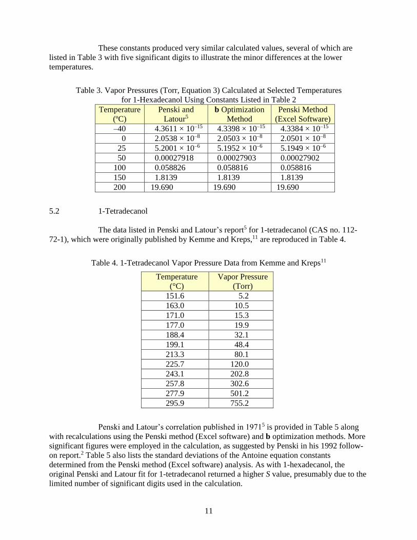
These constants produced very similar calculated values, several of which are
listed in Table 3 with five significant digits to illustrate the minor differences at the lower
temperatures.
Table 3. Vapor Pressures (Torr, Equation 3) Calculated at Selected Temperatures
for 1-Hexadecanol Using Constants Listed in Table 2
Temperature
(ºC)
Penski and
Latour5
b Optimization
Method
Penski Method
(Excel Software)
–40 4.3611 × 10⁻¹⁵ 4.3398 × 10⁻¹⁵ 4.3384 × 10⁻¹⁵
0 2.0538 × 10⁻⁸ 2.0503 × 10⁻⁸ 2.0501 × 10⁻⁸
25 5.2001 × 10⁻⁶ 5.1952 × 10⁻⁶ 5.1949 × 10⁻⁶
50 0.00027918 0.00027903 0.00027902
100 0.058826 0.058816 0.058816
150 1.8139 1.8139 1.8139
200 19.690 19.690 19.690
5.2 1-Tetradecanol
The data listed in Penski and Latour’s report5 for 1-tetradecanol (CAS no. 112-
72-1), which were originally published by Kemme and Kreps,11 are reproduced in Table 4.
Table 4. 1-Tetradecanol Vapor Pressure Data from Kemme and Kreps11
Temperature
(°C)
Vapor Pressure
(Torr)
151.6 5.2
163.0 10.5
171.0 15.3
177.0 19.9
188.4 32.1
199.1 48.4
213.3 80.1
225.7 120.0
243.1 202.8
257.8 302.6
277.9 501.2
295.9 755.2
Penski and Latour’s correlation published in 19715 is provided in Table 5 along
with recalculations using the Penski method (Excel software) and b optimization methods. More
significant figures were employed in the calculation, as suggested by Penski in his 1992 follow-
on report.2 Table 5 also lists the standard deviations of the Antoine equation constants
determined from the Penski method (Excel software) analysis. As with 1-hexadecanol, the
original Penski and Latour fit for 1-tetradecanol returned a higher S value, presumably due to the
limited number of significant digits used in the calculation.
12
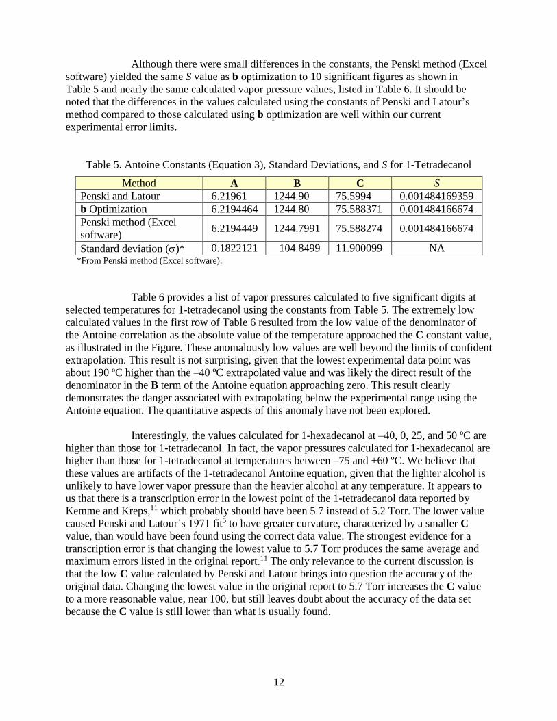
Although there were small differences in the constants, the Penski method (Excel
software) yielded the same S value as b optimization to 10 significant figures as shown in
Table 5 and nearly the same calculated vapor pressure values, listed in Table 6. It should be
noted that the differences in the values calculated using the constants of Penski and Latour’s
method compared to those calculated using b optimization are well within our current
experimental error limits.
Table 5. Antoine Constants (Equation 3), Standard Deviations, and S for 1-Tetradecanol
Method A B C S
Penski and Latour 6.21961 1244.90 75.5994 0.001484169359
b Optimization 6.2194464 1244.80 75.588371 0.001484166674
Penski method (Excel
software) 6.2194449 1244.7991 75.588274 0.001484166674
Standard deviation ()* 0.1822121 104.8499 11.900099 NA *From Penski method (Excel software).
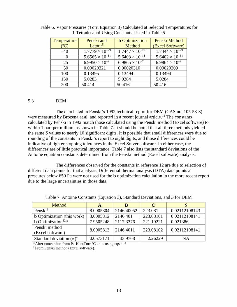
Table 6 provides a list of vapor pressures calculated to five significant digits at
selected temperatures for 1-tetradecanol using the constants from Table 5. The extremely low
calculated values in the first row of Table 6 resulted from the low value of the denominator of
the Antoine correlation as the absolute value of the temperature approached the C constant value,
as illustrated in the Figure. These anomalously low values are well beyond the limits of confident
extrapolation. This result is not surprising, given that the lowest experimental data point was
about 190 ºC higher than the –40 ºC extrapolated value and was likely the direct result of the
denominator in the B term of the Antoine equation approaching zero. This result clearly
demonstrates the danger associated with extrapolating below the experimental range using the
Antoine equation. The quantitative aspects of this anomaly have not been explored.
Interestingly, the values calculated for 1-hexadecanol at –40, 0, 25, and 50 ºC are
higher than those for 1-tetradecanol. In fact, the vapor pressures calculated for 1-hexadecanol are
higher than those for 1-tetradecanol at temperatures between –75 and +60 ºC. We believe that
these values are artifacts of the 1-tetradecanol Antoine equation, given that the lighter alcohol is
unlikely to have lower vapor pressure than the heavier alcohol at any temperature. It appears to
us that there is a transcription error in the lowest point of the 1-tetradecanol data reported by
Kemme and Kreps,11 which probably should have been 5.7 instead of 5.2 Torr. The lower value
caused Penski and Latour’s 1971 fit5 to have greater curvature, characterized by a smaller C
value, than would have been found using the correct data value. The strongest evidence for a
transcription error is that changing the lowest value to 5.7 Torr produces the same average and
maximum errors listed in the original report.11 The only relevance to the current discussion is
that the low C value calculated by Penski and Latour brings into question the accuracy of the
original data. Changing the lowest value in the original report to 5.7 Torr increases the C value
to a more reasonable value, near 100, but still leaves doubt about the accuracy of the data set
because the C value is still lower than what is usually found.
13
Table 6. Vapor Pressures (Torr, Equation 3) Calculated at Selected Temperatures for
1-Tetradecanol Using Constants Listed in Table 5
Temperature
(ºC)
Penski and
Latour5
b Optimization
Method
Penski Method
(Excel Software)
–40 1.7779 × 10⁻²⁹ 1.7447 × 10⁻²⁹ 1.7444 × 10⁻²⁹
0 5.6565 × 10⁻¹¹ 5.6403 × 10⁻¹¹ 5.6402 × 10⁻¹¹
25 6.9950 × 10⁻⁷ 6.9865 × 10⁻⁷ 6.9864 × 10⁻⁷
50 0.00020321 0.00020310 0.00020309
100 0.13495 0.13494 0.13494
150 5.0283 5.0284 5.0284
200 50.414 50.416 50.416
5.3 DEM
The data listed in Penski’s 1992 technical report for DEM (CAS no. 105-53-3)
were measured by Brozena et al. and reported in a recent journal article.12 The constants
calculated by Penski in 1992 match those calculated using the Penski method (Excel software) to
within 1 part per million, as shown in Table 7. It should be noted that all three methods yielded
the same S values to nearly 10 significant digits. It is possible that small differences were due to
rounding of the constants in Penski’s report to eight digits, and those differences could be
indicative of tighter stopping tolerances in the Excel Solver software. In either case, the
differences are of little practical importance. Table 7 also lists the standard deviations of the
Antoine equation constants determined from the Penski method (Excel software) analysis.
The differences observed for the constants in reference 12 are due to selection of
different data points for that analysis. Differential thermal analysis (DTA) data points at
pressures below 650 Pa were not used for the b optimization calculation in the more recent report
due to the large uncertainties in those data.
Table 7. Antoine Constants (Equation 3), Standard Deviations, and S for DEM
Method A B C S
Penski2 8.0005804 2146.40052 223.081 0.02112108143
b Optimization (this work) 8.0005812 2146.401 223.08101 0.02112108141
b Optimization12* 7.9505248 2117.3376 221.19221 0.021386
Penski method
(Excel software) 8.0005813 2146.4011 223.08102 0.02112108141
Standard deviation ()† 0.0573171 33.9768 2.26229 NA *After conversion from Pa-K to Torr-ºC units using eqs 4–6. † From Penski method (Excel software).
14
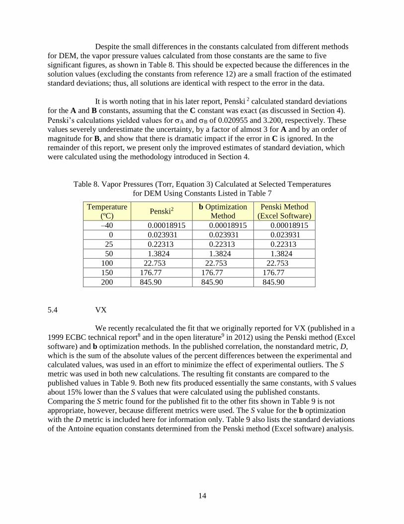
Despite the small differences in the constants calculated from different methods
for DEM, the vapor pressure values calculated from those constants are the same to five
significant figures, as shown in Table 8. This should be expected because the differences in the
solution values (excluding the constants from reference 12) are a small fraction of the estimated
standard deviations; thus, all solutions are identical with respect to the error in the data.
It is worth noting that in his later report, Penski 2 calculated standard deviations
for the A and B constants, assuming that the C constant was exact (as discussed in Section 4).
Penski’s calculations yielded values for A and B of 0.020955 and 3.200, respectively. These
values severely underestimate the uncertainty, by a factor of almost 3 for A and by an order of
magnitude for B, and show that there is dramatic impact if the error in C is ignored. In the
remainder of this report, we present only the improved estimates of standard deviation, which
were calculated using the methodology introduced in Section 4.
Table 8. Vapor Pressures (Torr, Equation 3) Calculated at Selected Temperatures
for DEM Using Constants Listed in Table 7
Temperature
(ºC) Penski2
b Optimization
Method
Penski Method
(Excel Software)
–40 0.00018915 0.00018915 0.00018915
0 0.023931 0.023931 0.023931
25 0.22313 0.22313 0.22313
50 1.3824 1.3824 1.3824
100 22.753 22.753 22.753
150 176.77 176.77 176.77
200 845.90 845.90 845.90
5.4 VX
We recently recalculated the fit that we originally reported for VX (published in a
1999 ECBC technical report8 and in the open literature9 in 2012) using the Penski method (Excel
software) and b optimization methods. In the published correlation, the nonstandard metric, D,
which is the sum of the absolute values of the percent differences between the experimental and
calculated values, was used in an effort to minimize the effect of experimental outliers. The S
metric was used in both new calculations. The resulting fit constants are compared to the
published values in Table 9. Both new fits produced essentially the same constants, with S values
about 15% lower than the S values that were calculated using the published constants.
Comparing the S metric found for the published fit to the other fits shown in Table 9 is not
appropriate, however, because different metrics were used. The S value for the b optimization
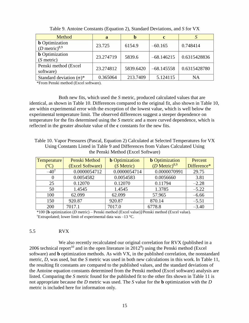
with the D metric is included here for information only. Table 9 also lists the standard deviations
of the Antoine equation constants determined from the Penski method (Excel software) analysis.
15
Table 9. Antoine Constants (Equation 2), Standard Deviations, and S for VX
Method a b c S
b Optimization
(D metric)8,9 23.725 6154.9 –60.165 0.748414
b Optimization
(S metric) 23.274719 5839.6 –68.146215 0.6315428836
Penski method (Excel
software) 23.274812 5839.6420 –68.145558 0.6315428780
Standard deviation ()* 0.365064 213.7409 5.124115 NA *From Penski method (Excel software).
Both new fits, which used the S metric, produced calculated values that are
identical, as shown in Table 10. Differences compared to the original fit, also shown in Table 10,
are within experimental error with the exception of the lowest value, which is well below the
experimental temperature limit. The observed differences suggest a steeper dependence on
temperature for the fits determined using the S metric and a more curved dependence, which is
reflected in the greater absolute value of the c constants for the new fits.
Table 10. Vapor Pressures (Pascal, Equation 2) Calculated at Selected Temperatures for VX
Using Constants Listed in Table 9 and Differences from Values Calculated Using
the Penski Method (Excel Software)
Temperature
(ºC)
Penski Method
(Excel Software)
b Optimization
(S Metric)
b Optimization
(D Metric)8,9
Percent
Difference*
–40† 0.0000054712 0.0000054714 0.0000070991 29.75
0 0.0054582 0.0054583 0.0056660 3.81
25 0.12070 0.12070 0.11794 –2.28
50 1.4545 1.4545 1.3785 –5.22
100 62.099 62.099 57.965 –6.66
150 920.87 920.87 870.14 –5.51
200 7017.1 7017.0 6778.8 –3.40 *100·[b optimization (D metric) – Penski method (Excel value)]/Penski method (Excel value). †Extrapolated; lower limit of experimental data was –13 °C.
5.5 RVX
We also recently recalculated our original correlation for RVX (published in a
2006 technical report10 and in the open literature in 20129) using the Penski method (Excel
software) and b optimization methods. As with VX, in the published correlation, the nonstandard
metric, D, was used, but the S metric was used in both new calculations in this work. In Table 11,
the resulting fit constants are compared to the published values, and the standard deviations of
the Antoine equation constants determined from the Penski method (Excel software) analysis are
listed. Comparing the S metric found for the published fit to the other fits shown in Table 11 is
not appropriate because the D metric was used. The S value for the b optimization with the D
metric is included here for information only.
16
Table 11. Antoine Constants (Equation 2), Standard Deviations, and S for RVX
Method a b c S
Excel software
(D metric)9,10 24.136 6464.0 –55.271 0.08878
b Optimization
(S metric) 23.806112 6269.8 –59.493359 0.08515025789
Penski method (Excel
software) 23.806171 6269.8357 –59.492558 0.08515025782
Standard deviation ()* 0.485769 297.1876 6.684891 NA *From Penski method (Excel software).
Values calculated at selected temperatures using the constants in Table 11 are
listed in Table 12, which also shows the agreement between the new b optimization results and
those generated using the Penski method (Excel software). All differences in calculated values
are within the current experimental error limits, except for the lowest value, which was
extrapolated well below the experimental temperature range.
Table 12. Vapor Pressures (Pascal, Equation 2) Calculated at Selected
Temperatures for RVX Using Constants Listed in Table 11
Temperature
(ºC)
Penski Method
(Excel Software)
b Optimization
(S Metric)
b Optimization
(D Metric)
Percent
Difference*
–40† 0.0000045588 0.0000045587 0.0000050138 9.98
0 0.0039301 0.0039301 0.0039587 0.73
25 0.085000 0.085000 0.083905 –1.29
50 1.0263 1.0263 1.0057 –2.00
100 45.456 45.456 44.756 –1.54
150 709.90 709.90 709.82 –0.01
200 5705.0 5705.0 5810.4 1.85 *100·(b optimization (D metric) – Penski method (Excel value))/Penski method (Excel value). †Extrapolated; lower limit of experimental data was –10 °C.
5.6 TDG
We recalculated our recently published TDG (CAS no. 111-48-8) correlation
using the Penski method (Excel software) and the data as they appear in that report.3 The
resulting fit constants are close to the published values, obtained using the b optimization
method with the S metric, as shown in Table 13. The differences between the published and new
b optimization results are attributed to the difficulty associated with finding the best solution
using the b optimization method. Table 13 also lists the standard deviations of the Antoine
equation constants that were determined from the Penski method (Excel software) analysis.
17
Table 13. Antoine Constants (Equation 2), Standard Deviations, and S for TDG
Method a b c S
b Optimization
(S metric)3 24.3482 6224.0 –67.9546 0.01235505437
b Optimization
(S metric, this work) 24.348076 6223.9 –67.956992 0.01235504204
Penski method
(Excel software) 24.348102 6223.9147 –67.956676 0.01235504202
Standard deviation ()* 0.411409 262.6135 6.323227 NA *From Penski method (Excel software).
These constants produced similar calculated values, several of which are listed in
Table 14 with five significant digits to illustrate small differences. In each case, there are no
differences between the new b optimization and the Penski method (Excel software) results, and
the differences between those and the published correlation values are all less than 0.01%. The
standard deviation estimates also indicate that all solutions are identical to within the error limits
of the experimental data.
Table 14. Vapor Pressures (Pascal, Equation 2) Calculated at Selected Temperatures
for TDG Using Constants Listed in Table 13
Temperature
(ºC)
Penski Method
(Excel Software)
b Optimization
(S Metric, This Work)
b Optimization
(S Metric3)
–40 0.0000016275 0.0000016275 0.0000016276
0 0.0025191 0.0025191 0.0025191
25 0.067903 0.067903 0.067901
50 0.95991 0.95991 0.95987
100 52.183 52.183 52.180
150 921.03 921.03 920.99
200 8004.4 8004.4 8004.1
5.7 N,N′-Diisopropylcarbodiimide (DICDI)
Our most recent report13 details the vapor pressure of DICDI (CAS no. 693-13-0),
which was determined using constants calculated via the b optimization method with the S
metric. Recalculation of the correlation using the Penski method (Excel software) produced
results (shown in Table 15) that reveal the fit described in reference 13 is nearly identical to the
one obtained using the Penski method (Excel software). Table 15 also lists the standard
deviations of the Antoine equation constants that were determined from the Penski method
(Excel software) analysis.
18
Table 15. Antoine Constants (Equation 2), Standard Deviations, and S for DICDI
Method a b c S
b Optimization13 20.78393 3214.75 –73.96220 0.001117473101
Penski method
(Excel software) 20.783935 3214.7534 –73.962050 0.001117473100
Standard deviation ()* 0.267660 142.8454 5.846359 NA *From Penski method (Excel software).
The vapor pressure values calculated using these constants are the same, to five
digits, as those shown in Table 16. This result demonstrates again that the b optimization method
can produce results comparable to those produced using the Penski method (Excel software), as
long as the same metric is used and the b optimization method is reliable for the particular data
set.
Table 16. Vapor Pressures (Pascal, Equation 2) Calculated at Selected
Temperatures for DICDI Using Constants Listed in Table 15
Temperature
(ºC)
Penski Method
(Excel Software)
b Optimization
(S Metric)13
–40 1.8026 1.8026
0 104.03 104.03
25 629.16 629.16
50 2651.9 2651.9
100 22903 22903
150 106680 106680
200 337970 337970
Although the b optimization method and the Penski method (Excel software) can
yield nearly identical results when the S metric is used, the former is more tedious and can give
lower-quality fits in unfavorable cases. It is not clear to us whether those lower-quality fits are a
result of the amount and quality of the data, the experience of the user, a combination of factors,
or some other cause. It appears that the Penski method (Excel software) is consistently superior
to the b optimization method because all data analyzed to date have yielded a smaller S when the
Penski method was used.
We intend to use the Penski method (Excel software) with the S metric for future
vapor pressure data correlations. Because viscosity data may also be correlated using the Antoine
equation and similar procedures, it is likely that those correlations will also be improved by use
of this method.
Table 17 lists the standard deviations of the Antoine constants from the tables in
this report. The standard deviations for the three compounds studied by Penski and Latour were
converted to enable direct comparisons. The table also includes the number of data points used
for each analysis. It is clear from Table 17 that the compound with the greatest number of data
points (DEM) had the smallest standard deviation for all three constants. When more data points
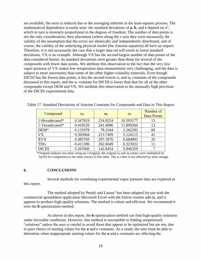
19
are available, the error is reduced due to the averaging inherent in the least-squares process. The
mathematical dependence is easily seen: the standard deviations of a, b, and c depend on σ2,
which in turn is inversely proportional to the degrees of freedom. The number of data points is
not the only consideration; their placement (where along the x axis they were measured), the
validity of the assumption that the errors are identically and independently distributed, and of
course, the validity of the underlying physical model (the Antoine equation) all have an impact.
Therefore, it is not necessarily the case that a larger data set will result in lower standard
deviations. VX is an example. Although VX has the second-largest number of data points of the
data considered herein, its standard deviations were greater than those for several of the
compounds with fewer data points. We attribute this observation to the fact that the very low
vapor pressure of VX makes low-temperature data measurement very challenging, and the data is
subject to more uncertainty than some of the other higher-volatility materials. Even though
DICDI has the fewest data points, it has the second lowest σa and σb constants of the compounds
discussed in this report, and the σc constant for DICDI is lower than that for all of the other
compounds except DEM and VX. We attribute this observation to the unusually high precision
of the DICDI experimental data.
Table 17. Standard Deviations of Antoine Constants for Compounds and Data in This Report
Compound σa σb σc Number of
Data Points
1-Hexadecanol* 0.347819 254.9254 10.593177 13
1-Tetradecanol* 0.419529 241.4086 11.899260 12
DEM* 0.131978 78.2344 2.262292 66
VX 0.365064 213.7409 5.124115 41
RVX 0.485769 297.1876 6.684891 20
TDG 0.411396 262.6049 6.323022 11
DICDI 0.267660 142.8454 5.846359 7 *Original analysis was done using eq 3 (log(p)); the original σa and σb values were multiplied by
ln(10) for comparison to the other entries in this table. The σc value is not affected by units change.
6. CONCLUSIONS
Several methods for correlating experimental vapor pressure data are explored in
this report.
The method adopted by Penski and Latour5 has been adapted for use with the
commercial spreadsheet application Microsoft Excel with the Solver routine add-in, and it
appears to produce high-quality solutions. The method is robust and efficient. We recommend it
over the b optimization method.
As shown in this report, the b optimization method can find high-quality solutions
under favorable conditions. However, this method is susceptible to finding unoptimized
“solutions” unless the user is careful to avoid those that appear to be optimized but are not, due
to poor choice of starting values for the a and c constants. As a result, the user must be able to
determine when inappropriate starting values for the a and c constants are affecting the
20
optimization process. This can be done most easily by plotting the c versus S results in real time
to ensure that a smooth curve is obtained. The b optimization method is tedious, requiring
manual variation of the b constant while a and c are allowed to vary until a minimum S is
determined.
The Antoine constants published previously for VX and RVX8–10 are numerically
different than those obtained using the Penski method (Excel software). The published fits were
both based on the D optimization metric, and a direct comparison of Antoine constants to those
determined using the S metric is not appropriate.
In this report, we also present a statistical analysis of the least-squares fitting of
the Antoine equation. Penski had presented estimates for the standard deviations of the a and b
parameters, but these were based on the erroneous assumption that the c coefficient was known
exactly. We present updated equations derived from least-squares theory to more properly
estimate the standard deviations of all three solution parameters. For DEM, we show that
Penski’s standard deviations underestimated the error by a factor of 3 in the case of the a
parameter and by a factor of 10 in the case of the b parameter. Although we endorse Penski and
Latour’s method, we emphasize that their equations for the standard error5 should be replaced by
those discussed in this report.
Analysis of Antoine constants determined for the compounds and data in this
report shows that the various methods generally succeed at finding the same effective solution.
Differences in the solution values tend to be very small fractions of the standard deviations of the
solution coefficients, and thus are effectively identical. The standard deviations of the solution
parameters are also useful to compare the quality of different data sets.
21
LITERATURE CITED
1. Thomson, G.W. The Antoine Equation for Vapor-Pressure Data. Chem. Rev. 1946, 38, 1–39.
2. Penski, E.C. Vapor Pressure Data Analysis Methodology, Statistics, and Applications;
CRDEC-TR-386; U.S. Army Chemical Research, Development, and Engineering Center:
Aberdeen Proving Ground, MD, 1992; UNCLASSIFIED Report (ADA255090).
3. Brozena, A.; Tevault, D.E.; Irwin, K. Vapor Pressure of Thiodiglycol. J. Chem. Eng. Data
2014, 59, 307–311.
4. Bauer, H.; Burschkies, K. Sattigungsdrucke einiger Senfole und Sulfide. Chem. Ber. 1935, 68
(6), 1238−1243.
5. Penski, E.P.; Latour, Jr., L.J. Conversational Computation Method for Fitting the Antoine
Equation to Vapor-Pressure-Temperature Data; EATR 4491; U.S. Army Chemical Research
Laboratory: Edgewood Arsenal, Aberdeen Proving Ground, MD, 1971; UNCLASSIFIED Report
(AD881829).
6. Seber, G.A.F.; Wild, C.J. Nonlinear Regression, John Wiley and Sons: Hoboken, NJ, 2003.
7. Tevault, D. Vapor Pressure Data Analysis and Correlation Methodology for Data Spanning
the Melting Point; ECBC-CR-135; U.S. Army Edgewood Chemical Biological Center: Aberdeen
Proving Ground, MD, 2013; UNCLASSIFIED Report (ADA592605).
8. Buchanan, J.H.; Butrow, A.B.; Abercrombie, P.L.; Buettner, L.C.; Tevault, D.E. Vapor
Pressure of VX; ECBC-TR-068; U.S. Army Edgewood Chemical Biological Center: Aberdeen
Proving Ground, MD, 1999; UNCLASSIFIED Report (ADA371297).
9. Tevault, D.E.; Brozena, A.; Buchanan, J.H.; Abercrombie-Thomas, P.L.; Buettner, L.C.
Thermophysical Properties of VX and RVX. J. Chem. Eng. Data 2012, 57, 1970–1977.
10. Buchanan, J.H.; Butrow, A.B.; Abercrombie, P.L.; Buettner, L.C.; Tevault, D.E. Vapor
Pressure of Russian VX; ECBC-TR-480; U.S. Army Edgewood Chemical Biological Center:
Aberdeen Proving Ground, MD, 2006; UNCLASSIFIED Report (ADA447993).
11. Kemme, H.R.; Kreps, S.I. Vapor Pressure of Primary n-Alkyl Chlorides and Alcohols.
J. Chem. Eng. Data 1969, 14, 98–102.
12. Brozena, A.; Buchanan, J.B.; Miles, Jr., R.W.; Williams, B.R.; Hulet, M.S. Vapor Pressure of
Triethyl and Tri-n-Propyl Phosphates and Diethyl Malonate. J. Chem. Eng. Data 2014, 59,
2649–2659.
13. Brozena, A.; Williams, B.R.; Tevault, D.E. Vapor Pressure of N,N΄-
Diisopropylcarbodiimide; ECBC-TR-1352; U.S. Army Edgewood Chemical Biological Center:
Aberdeen Proving Ground, MD, 2006; UNCLASSIFIED Report.

22
Blank
23
ACRONYMS AND ABBREVIATIONS
CAS Chemical Abstracts Service
Csat saturation concentration
ΔHvap enthalpy of vaporization
DEM diethyl malonate
DICDI N,N′-diisopropylcarbodiimide
DTA differential thermal analysis
ECBC U.S. Army Edgewood Chemical Biological Center
P vapor pressure (Pa)
p vapor pressure (Torr)
R ideal gas constant
RVX O-isobutyl-S-[2(diethylamino)ethyl] methylphosphonothiolate
T absolute temperature (K)
t temperature (°C)
TDG thiodiglycol
VX O-ethyl S-(2-diisopropylaminoethyl) methylphosphonothiolate

24
Blank
25
APPENDIX
SCREENSHOTS OF MICROSOFT EXCEL TEMPLATE
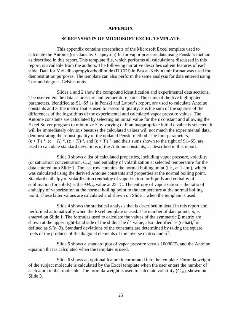
This appendix contains screenshots of the Microsoft Excel template used to
calculate the Antoine (or Clausius–Clapeyron) fit for vapor pressure data using Penski’s method
as described in this report. This template file, which performs all calculations discussed in this
report, is available from the authors. The following narrative describes salient features of each
slide. Data for N,N′-diisopropylcarbodiimide (DICDI) in Pascal-Kelvin unit format was used for
demonstration purposes. The template can also perform the same analysis for data entered using
Torr and degrees Celsius units.
Slides 1 and 2 show the compound identification and experimental data sections.
The user enters the data as pressure and temperature pairs. The sums of the five highlighted
parameters, identified as S1–S5 as in Penski and Latour’s report, are used to calculate Antoine
constants and S, the metric that is used to assess fit quality. S is the sum of the squares of the
differences of the logarithms of the experimental and calculated vapor pressure values. The
Antoine constants are calculated by selecting an initial value for the c constant and allowing the
Excel Solver program to minimize S by varying c. If an inappropriate initial c value is selected, it
will be immediately obvious because the calculated values will not match the experimental data,
demonstrating the robust quality of the updated Penski method. The four parameters,
(c + Ti)–1, (c + Ti)
–2, (c + Ti)–3, and (c + Ti)
–4, and their sums shown to the right of S1–S5, are
used to calculate standard deviations of the Antoine constants, as described in this report.
Slide 3 shows a list of calculated properties, including vapor pressure, volatility
(or saturation concentration, Csat), and enthalpy of volatilization at selected temperature for the
data entered into Slide 1. The last row contains the normal boiling point (i.e., at 1 atm), which
was calculated using the derived Antoine constants and properties at the normal boiling point.
Standard enthalpy of volatilization (enthalpy of vaporization for liquids and enthalpy of
sublimation for solids) is the Hvap value at 25 °C. The entropy of vaporization is the ratio of
enthalpy of vaporization at the normal boiling point to the temperature at the normal boiling
point. These latter values are calculated and shown on Slide 1 when the template is used.
Slide 4 shows the statistical analysis that is described in detail in this report and
performed automatically when the Excel template is used. The number of data points, n, is
entered on Slide 1. The formulas used to calculate the values of the symmetric matrix are
shown at the upper right-hand side of the slide. The 2 value, also identified as (-hat),2 is
defined as S/(n–3). Standard deviations of the constants are determined by taking the square
roots of the products of the diagonal elements of the inverse matrix and 2.
Slide 5 shows a standard plot of vapor pressure versus 10000/TK and the Antoine
equation that is calculated when the template is used.
Slide 6 shows an optional feature incorporated into the template. Formula weight
of the subject molecule is calculated by the Excel template when the user enters the number of
each atom in that molecule. The formula weight is used to calculate volatility (Csat), shown on
Slide 3.
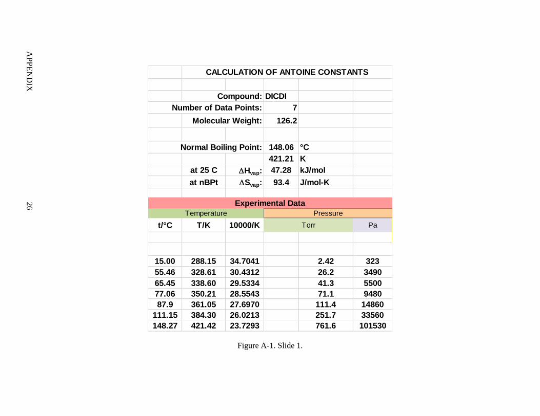
Figure A-1. Slide 1.
DICDI
7
Molecular Weight: 126.2
148.06 °C
421.21 K
at 25 C Hvap: 47.28 kJ/mol
at nBPt Svap: 93.4 J/mol-K
t/°C T/K 10000/K Pa
15.00 288.15 34.7041 2.42 323
55.46 328.61 30.4312 26.2 3490
65.45 338.60 29.5334 41.3 5500
77.06 350.21 28.5543 71.1 9480
87.9 361.05 27.6970 111.4 14860
111.15 384.30 26.0213 251.7 33560
148.27 421.42 23.7293 761.6 101530
Experimental Data
Temperature Pressure
Torr
Number of Data Points:
Normal Boiling Point:
Compound:
CALCULATION OF ANTOINE CONSTANTS
AP
PE
ND
IX 2
6
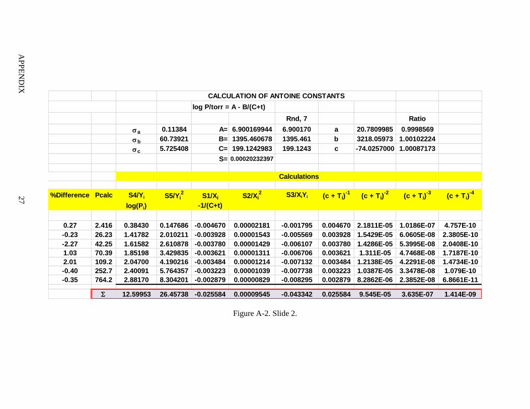
Figure A-2. Slide 2.
log P/torr = A - B/(C+t)
Rnd, 7 Ratio
a 0.11384 A= 6.900169944 6.900170 a 20.7809985 0.9998569
b 60.73921 B= 1395.460678 1395.461 b 3218.05973 1.00102224
c 5.725408 C= 199.1242983 199.1243 c -74.0257000 1.00087173
S= 0.00020232397
%Difference Pcalc S4/Yi S5/Yi2
S1/Xi S2/Xi2 S3/XiYi (c + Ti)
-1(c + Ti)
-2(c + Ti)
-3(c + Ti)
-4
log(Pi) -1/(C+t)
0.27 2.416 0.38430 0.147686 -0.004670 0.00002181 -0.001795 0.004670 2.1811E-05 1.0186E-07 4.757E-10
-0.23 26.23 1.41782 2.010211 -0.003928 0.00001543 -0.005569 0.003928 1.5429E-05 6.0605E-08 2.3805E-10
-2.27 42.25 1.61582 2.610878 -0.003780 0.00001429 -0.006107 0.003780 1.4286E-05 5.3995E-08 2.0408E-10
1.03 70.39 1.85198 3.429835 -0.003621 0.00001311 -0.006706 0.003621 1.311E-05 4.7468E-08 1.7187E-10
2.01 109.2 2.04700 4.190216 -0.003484 0.00001214 -0.007132 0.003484 1.2138E-05 4.2291E-08 1.4734E-10
-0.40 252.7 2.40091 5.764357 -0.003223 0.00001039 -0.007738 0.003223 1.0387E-05 3.3478E-08 1.079E-10
-0.35 764.2 2.88170 8.304201 -0.002879 0.00000829 -0.008295 0.002879 8.2862E-06 2.3852E-08 6.8661E-11
12.59953 26.45738 -0.025584 0.00009545 -0.043342 0.025584 9.545E-05 3.635E-07 1.414E-09
Calculations
CALCULATION OF ANTOINE CONSTANTS
AP
PE
ND
IX 2
7
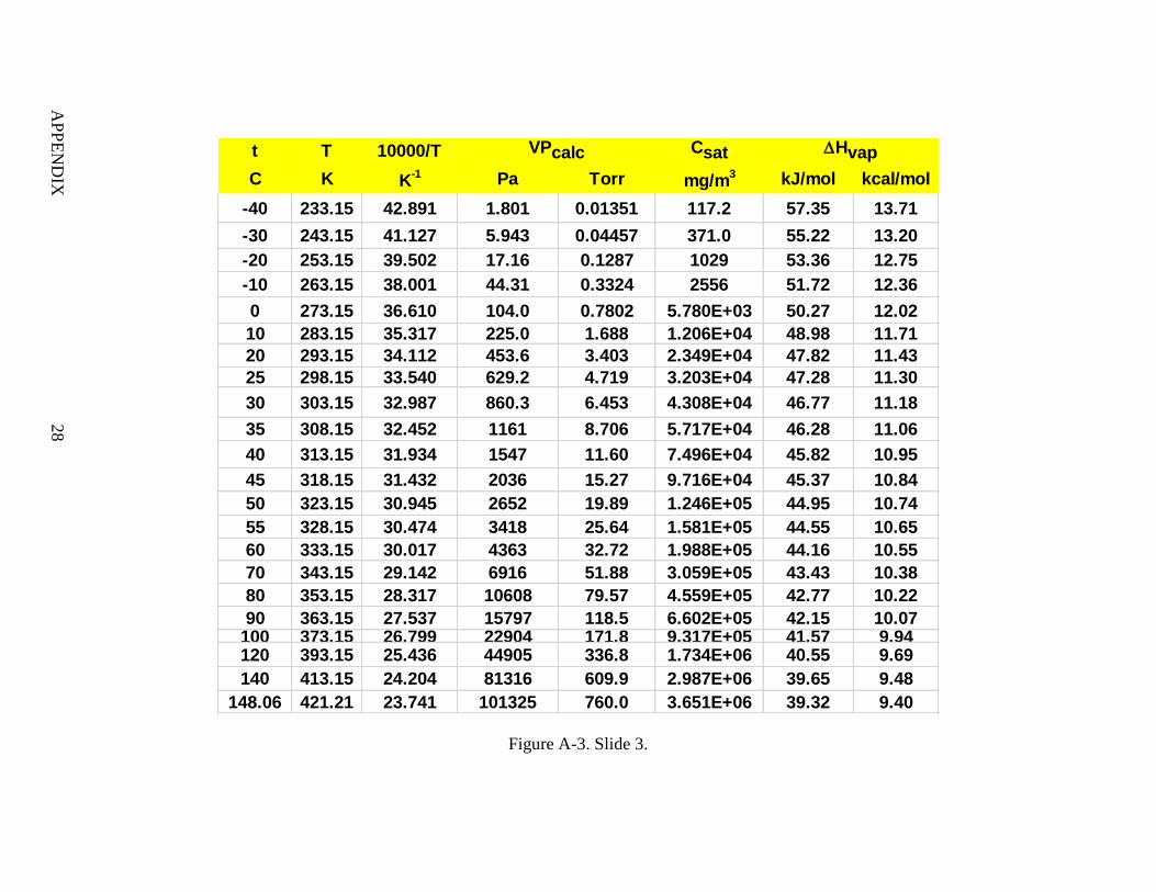
Figure A-3. Slide 3.
t T 10000/T Csat
C K K-1 Pa Torr mg/m
3 kJ/mol kcal/mol
-40 233.15 42.891 1.801 0.01351 117.2 57.35 13.71
-30 243.15 41.127 5.943 0.04457 371.0 55.22 13.20
-20 253.15 39.502 17.16 0.1287 1029 53.36 12.75
-10 263.15 38.001 44.31 0.3324 2556 51.72 12.36
0 273.15 36.610 104.0 0.7802 5.780E+03 50.27 12.02
10 283.15 35.317 225.0 1.688 1.206E+04 48.98 11.71
20 293.15 34.112 453.6 3.403 2.349E+04 47.82 11.43
25 298.15 33.540 629.2 4.719 3.203E+04 47.28 11.30
30 303.15 32.987 860.3 6.453 4.308E+04 46.77 11.18
35 308.15 32.452 1161 8.706 5.717E+04 46.28 11.06
40 313.15 31.934 1547 11.60 7.496E+04 45.82 10.95
45 318.15 31.432 2036 15.27 9.716E+04 45.37 10.84
50 323.15 30.945 2652 19.89 1.246E+05 44.95 10.74
55 328.15 30.474 3418 25.64 1.581E+05 44.55 10.65
60 333.15 30.017 4363 32.72 1.988E+05 44.16 10.55
70 343.15 29.142 6916 51.88 3.059E+05 43.43 10.38
80 353.15 28.317 10608 79.57 4.559E+05 42.77 10.22
90 363.15 27.537 15797 118.5 6.602E+05 42.15 10.07100 373.15 26.799 22904 171.8 9.317E+05 41.57 9.94120 393.15 25.436 44905 336.8 1.734E+06 40.55 9.69
140 413.15 24.204 81316 609.9 2.987E+06 39.65 9.48
148.06 421.21 23.741 101325 760.0 3.651E+06 39.32 9.40
VPcalc Hvap
AP
PE
ND
IX 2
8
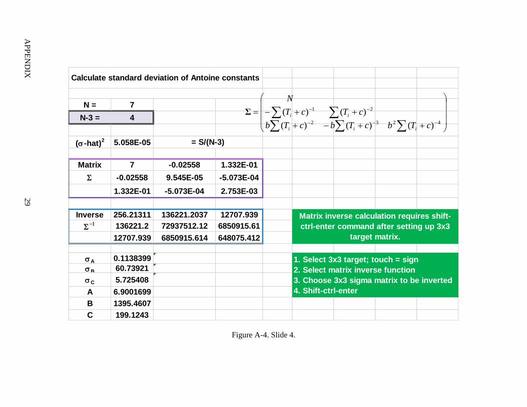
Figure A-4. Slide 4.
N = 7
N-3 = 4
(-hat)2 5.058E-05
Matrix 7 -0.02558 1.332E-01
-0.02558 9.545E-05 -5.073E-04
1.332E-01 -5.073E-04 2.753E-03
Inverse 256.21311 136221.2037 12707.939
136221.2 72937512.12 6850915.61
12707.939 6850915.614 648075.412
%
A 0.1138399 #DIV/0!
B 60.73921 #DIV/0!
C 5.725408 #DIV/0!
A 6.9001699
B 1395.4607
C 199.1243
= S/(N-3)
Calculate standard deviation of Antoine constants
1. Select 3x3 target; touch = sign
2. Select matrix inverse function
3. Choose 3x3 sigma matrix to be inverted
4. Shift-ctrl-enter
Matrix inverse calculation requires shift-
ctrl-enter command after setting up 3x3
target matrix.
4232
21
)()()(
)()(
cTbcTbcTb
cTcT
N
iii
iiΣ
AP
PE
ND
IX 2
9
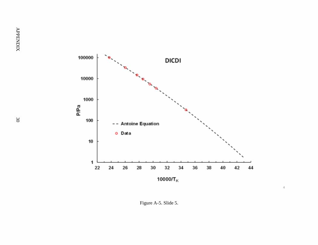
Figure A-5. Slide 5.
AP
PE
ND
IX 3
0
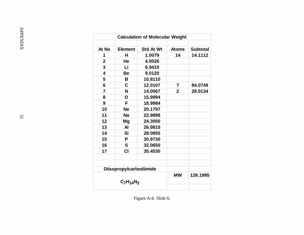
Figure A-6. Slide 6.
At No Element Std At Wt Atoms Subtotal
1 H 1.0079 14 14.1112
2 He 4.0026
3 Li 6.9410
4 Be 9.0120
5 B 10.8110
6 C 12.0107 7 84.0749
7 N 14.0067 2 28.0134
8 O 15.9994
9 F 18.9984
10 Ne 20.1797
11 Na 22.9898
12 Mg 24.3050
13 Al 26.9815
14 Si 28.0855
15 P 30.9730
16 S 32.0650
17 Cl 35.4530
MW 126.1995
C7H14N2
Diisopropylcarbodiimide
Calculation of Molecular Weight
AP
PE
ND
IX 3
1

Blank
DISTRIBUTION LIST
The following individuals and organizations were provided with one Adobe
portable document format (pdf) electronic version of this report:
U.S. Army Edgewood Chemical
Biological Center (ECBC)
RDCB-DRC-P
ATTN: Brozena, A.
Ellzy, M.
Defense Threat Reduction Agency
J9-CBS
ATTN: Peacock-Clark, S.
Graziano, A.
Department of Homeland Security
DHS-S&T-RDP-CSAC
ATTN: Strang, P.
RDCB-PI-CSAC
ATTN: Negron, A.
G-3 History Office
U.S. Army RDECOM
ATTN: Smart, J.
Office of the Chief Counsel
AMSRD-CC
ATTN: Upchurch, V.
ECBC Rock Island
RDCB-DES
ATTN: Lee, K.
ECBC Technical Library
RDCB-DRB-BL
ATTN: Foppiano, S.
Stein, J.
Defense Technical Information Center
ATTN: DTIC OA