1

Valuing Time in Supply Chains: Establishing Limits of Time-based

Competition

Joseph Blackburn

James A. Speyer Professor of Operations Management

Owen Graduate School of Management

Vanderbilt University

Nashville, TN 37203 USA

2

Valuing Time in Supply Chains: Establishing Limits of Time-based

Competition

1. Introduction

Time-based competition entered the lexicon of operations strategy in 1988 with Stalk’s seminal

piece “Time—the Next Source of Competitive Advantage”. The central theme of a time-based

strategy is that an organization can achieve a powerful competitive advantage through speed: by

responding faster to customers, by faster development of new products and services, and by

faster movement of products through the supply chain (Stalk (1990), Blackburn (1991)). The

concept gained wide acceptance in the business world based on reports of firms building

successful business strategies around time-to-market for new products and speed of response for

services and products with variable demand.

Much of the early published work implied that there were few limits to time-based competition,

echoing a theme that “faster is better” (Schmenner, 1988). In Clockspeed Fine (1998) observed

that industries evolve at different speeds and that all competitive advantages based on speed were

temporary, particularly in fast clockspeed industries. Souza et al. (2004) observed that time-to-

market and industry clockspeed tend to be correlated, and Bayus (1997) raised the possibility

that firms could, at times, be too fast to market with innovative products.

Subsequent research has found more evidence of limits to time-based competition. The existence

of limits to speed for all processes should not be surprising because just as the laws of physics

impose limits on the speed of physical processes, economics principles establish limits for

business processes. Faster operations are desired only up to the tipping point at which the

marginal benefits from additional time reduction equals the marginal cost of the additional speed.

This marginal value of time (MVT) effectively defines the limits of time-based competition for a

process. These limits are not static, of course; they change over time with technology, level of

competition, and customer preferences—but they do exist.

The marginal value of time defines the limits of time-based competition for a service process. In

many service processes customer response time can be improved through investment in

technology and resources, but the limiting value for that investment is often determined by the

value customers place on their waiting time. An interesting application of this principle in the

3

fast-food industry is provided by Allon et al. (2011). They combined a model of customer

behavior with an experimental study of customer wait times to determine the value customers

place on waiting time, giving fast-food providers a measure of the marginal value of

improvements in response time.

Limits to time-based competition have also been studied in the reverse supply chain for

remanufactured products (Blackburn, 2004). Research in this industry found that speed is

particularly important in the asset recovery of some returned products, such as consumer

electronics, because these products experience rapidly deteriorating demand and loss of market

value over time. These firms should invest heavily in speed of product recovery. However,

firms whose products experience relatively stable demand (like the products studied in this

paper) will have low marginal value of time, implying lower benefits to speed of recovery.

These firms face stricter limits on time-based competition and should design their reverse supply

chain to reduce cost, rather than time.

This paper explores the economic limits of time-based competition through the lens of global

supply chains. Supply chains provide an excellent setting in which to define and explore limits

to time-based competitive advantage. Suppose a mass-market retailer is choosing where to

source products from their network of global suppliers. If sourced domestically, then the supply

chain would be short, stock replenishment times would be fast, but manufacturing costs could be

higher. If sourced offshore, the supply chain is longer, replenishment times become slower,

inventory costs rise, but component manufacturing costs are typically lower. A time-based (or

quick response) strategy would imply sourcing closer to home for faster replenishment.

The evidence strongly suggests that over the past several decades many supply chains have

become longer, and slower. The value of imports of merchandise from the People’s Republic of

China quintupled between 1997 and 2007 rising from $54 billion to $342 billion, which

represented 17% of all imported manufactured goods (Arnold, 2008). In its early days Wal-Mart

heralded that their merchandise was “Made in the USA”; today Wal-Mart is the largest single US

importer of goods from China. In manufacturing, entire domestic industries have been

“hollowed out” as production has moved offshore in search of lower production costs, yielding a

longer supply chain. The growth of global supply chains is time-based competition in reverse.

4

Supply chains pose the following conundrum for time-based competition: if time is so valuable,

then why are supply chains so long? If supply chains evolved like most other processes, they

would be getting shorter and faster, but in general they have not. Conventional wisdom suggests

that as replenishment times in the supply chain increase, inventory in the pipeline and in safety

stocks rises, and the cost of carrying these inventories must soar. Therefore supply chains should

be getting faster to offset these costs.

We address these questions by determining the MVT for a supply chain and using it to define the

limits of time-based competition in the sourcing of products. We consider a produce-to-stock

supply chain for functional products, which were defined by Fisher (1997) as products with

predictable demand and (relatively) long life cycles. For these products we develop analytical

expressions for MVT—that is, the change in inventory costs per unit change in supply-chain

lead-time under a wide variety of conditions—optimal and suboptimal reorder-point policies,

and deterministic and variable lead-times. Because the MVT is computed as the change in a

product’s unit cost per unit change in lead-time, the results do not depend on a given product’s

price and are therefore widely applicable across product categories.

The MVT helps resolve the conundrum. Our results show that for most supply chains the MVT

values are surprisingly low, even with high demand and lead-time variability, and therefore the

effect on product costs of increasing the lead-time are smaller than expected (as are the effects on

product costs of lead-time decreases). The significant implication of this is that only a small

reduction in manufacturing cost is required to offset the increase in inventory costs from a longer

supply chain. The low value of MVT has had a profound effect on the growth of global supply

chains for functional products.

This paper makes the following contributions. First, we establish limits to time-based

competition in a produce-to-stock supply chain by developing a generic marginal value of time

that is independent of product cost. Second, we derive expressions for computing the MVT

under a wide range of inventory policies—fixed and continuous review, deterministic and

stochastic lead-times, and optimal and suboptimal policies. We test the predictive accuracy of

these MVT expressions by comparing them to values obtained from simulations of actual

offshore supply chain applications. Third, and most importantly, we demonstrate that the MVT

tends to be very low—significantly less than 1 % of unit cost per week for most supply chains,

5

even those with highly-variable lead-times. These low MVT values provide an economic

rationale for the explosive growth in trans-oceanic supply chains and offshore sourcing.

2. Literature Review

The literature on time-based competition is extensive. Of that literature, the research studies

relevant to this paper have implicitly explored limits to time-based competition by quantifying

the value of faster response time in processes. Many early papers on faster response focused on

manufacturing processes. For example, Porteus (1985) explored the benefits of investing in

reducing the setup time for production runs. Handfield (1995) and Suri (1998) have documented

the benefits of quick response manufacturing and prescribed implementation methodology. In the

delivery of services So (2000) studied the relationship between price and time guarantees in a

competitive market. Lederer and Li (1997) and Shang and Liu (2011) have quantified the

benefits of faster delivery times for make-to-order products under competitive conditions.

Another line of research focuses on the value of quick response in the retailing of innovative, or

fashion, products (Fisher and Raman (1996), Iyer and Bergen (1997), and Caro and Martinez-de-

Albeniz (2010)). Due to short product life-cycles, this research has typically used a variant of

the newsboy problem to evaluate the value of better demand information or quicker response.

Our research is similar to this stream of research in its concern with the relationship between

time and costs in a make-to-stock supply chain. However, it is dissimilar in its focus on

functional, rather than innovative, products and its use of multi-period inventory models instead

of the newsboy model.

The growing body of research on cost models to evaluate sourcing decisions in global supply

chain management is also relevant for our study. In empirical studies of the inventory-driven

costs in supply chains, Lowson (2002), Callioni et al. (2005), and Holweg et al. (2011) have

found that traditional inventory costs constitute a small percentage of total sourcing costs. A

large proportion of sourcing costs were “hidden costs” (costs of coordination, currency

fluctuation, technical support, obsolescence, etc.) that are difficult to model. Hausman et al.

(2010) built a global trade process model for both innovative and functional products that they

validated with empirical data from a combination of sources. They used the model to predict the

cost savings from “IT-enabled” reductions in the supply chain lead-time. Upon close

examination, their results show that reductions in lead-time for traditional products are a tiny

6

fraction of the total cost savings. All these empirical studies lend qualitative support for our

findings concerning the relative importance of traditional inventory costs in a supply chain.

We also draw on traditional inventory model research, specifically research that examines the

relationship between the lead-time and total inventory cost for make-to-stock systems. Hill and

Khosla (1992) constructed a make-to-stock, continuous-review inventory model in which lead-

time is a decision variable and found the optimum reduction in lead-time. In Blackburn (2001)

we generalized Hill and Khosla’s model to include pipeline inventories and investigated the

effect on inventory costs of lead-time changes under optimal and sub-optimal polices. Bischak et

al. (2011) and Fang et al. (2011) have generalized these inventory models to consider stochastic

lead-times. Bischak et al. considered a periodic-review inventory model with gamma-distributed

demand and used simulation to investigate the effects on inventory costs of reducing lead-time

and lead-time variability. Fang et al. conducted an analytical study of a fixed-review period

model with normally-distributed demand and developed expressions to estimate the effect on

inventory costs of marginal changes in lead-time and lead-time variability.

Our model generalizes these prior models in two important ways. First, we develop a simplified

analytical approximation to total cost, using the normal distribution, that is applicable to both

periodic and continuous-review, backorders and lost sales, and optimal and suboptimal inventory

policies. Second, by transforming the metric from total cost to MVT as a percentage of product

unit cost, the results we obtain about the sensitivity of inventory costs to changes in lead-time

yield insights that are broadly applicable.

3. Model and Analysis: Marginal Value of Changes in Lead-Time

In this section we develop analytical models to quantify the effect on inventory costs of changes

in the replenishment lead-time in a make-to-stock supply chain. The upstream producer of a

product (or component) ships to a downstream inventory stocking point, which can be a

distribution center, a retailer, or an assembler of finished product (in the case of a component).

Demand at the stocking point is variable, and the products are assumed to be functional-- that is,

products have predictable demand and relatively long life cycles. Our inventory models do not

capture losses due to obsolescence or perishability, which would occur with innovative products,

such as high-fashion goods or fresh foods.

7

Inventory is managed through replenishment orders placed on the upstream producer using

conventional reorder-point models. We illustrate the development of our model assuming a

continuous-review policy in which unfilled demand is backlogged, then derive analogous cost

expressions for other reorder-point models. In the continuous-review model, when the

downstream inventory position (on-hand + on-order) falls below level r, an order Q is released to

the upstream supplier. The replenishment lead-time is L time periods-- the total time for

upstream production and delivery of the product to the stocking point. Demands by time period

are independent and normally distributed with mean µ and variance . As in Fang et al. (2011),

we assume that replenishment lead-times are independently, identically distributed with mean L

and standard deviation . and that demand per time unit is normally distributed. Then demand

over the replenishment interval is a random variable, X, with mean and standard deviation

√ .

The reorder point r equals Lµ + , or expected demand during lead-time + safety stock equal

to k standard deviations of demand. Hereafter, this inventory policy is denoted by (Q, k), and we

take the policy as given because our concern is with how total inventory costs change as the

lead-time, L, is changed, not with inventory policy selection. For greater generality we

specifically do not assume that (Q,k) are chosen optimally; we only assume that the firm

maintains a consistent policy (that is, constant k and Q) as L is changed.

Additional notation for the (Q,k) model is as follows:

A = Ordering cost;

D = Expected annual demand;

c = Unit cost of item;

i = Annual inventory carrying charge, as a fraction of the unit cost c;

p = Backorder (or shortage) cost/unit;

b= p/ic , the ratio of the shortage cost/annual carrying cost;

δ = ⁄ , the coefficient of variation of demand per time period;

B(Q,k,L) = average number of backorders outstanding.

8

To characterize the standard normal distribution in terms of k, let ( ) denote the pdf, ( ) the

cdf, (k)= (1- ( )) the complementary cdf, and the standard normal loss functions are

( ) =

k(x)dxk)-(x ; (k) =∫ ( )

[ ( ) ( ))] (see Zipkin, 2000).

Then the total annual expected cost of a (Q,k) inventory policy with lead-time L is

( ) ( ) [ ( )] ( ) ( ) (1)

Expression (1) is the sum, respectively, of the annual ordering cost and production cost, the

annual costs of inventory in the pipeline, average cycle stock, safety stock, the average quantity

on backorder, and the annual expected cost of backorders. If lead-time is deterministic (i.e.

√ ) , then expression (1) is the expected annual cost of a ( , )Q k policy as given in well-

known inventory management texts (see Hadley and Whitin (1963)), except that (1) also includes

the annual cost of inventory in the supply-chain pipeline ( ic L ).

3.1 The Marginal Value of Time in a Supply Chain

To quantify how inventory costs vary with changes in lead-time, we define the marginal value of

lead-time ( MVL ) as the partial derivative of TC with respect to L

( ) ( )[ ( ) ( )]

( )

(2)

Hill and Khosla (1992) developed an expression similar to (2) for the deterministic lead-time

case, but omitted the expected backorder cost and limited their analysis to lead-time reduction.

In this analysis we also consider increases in lead-time to quantify the cost effects of lengthening

the supply chain. However, by including the unit product cost c, expression (2) is restricted in

generality: it depends on, and is sensitive to, product costs, which precludes comparisons across

product categories and general statements about the marginal value of time in a supply chain.

To resolve this issue, we construct a more useful transformation of the expression by

simply dividing it by the annual cost of goods sold, . When defined as a percentage of the

product’s unit cost, the results are more general because time values can be compared across

product categories regardless of the cost of the product. For the transformation, we define the

function

as the “value of time”. equals the incremental change in inventory

9

costs of a unit change in the supply chain lead-time expressed as a fraction of the unit cost of the

product. The formal expression for MVT is derived from (2):

( ) (

) [ (

) ( ( ⁄ ) ( ))

( )

] (3)

In previous studies of supply chains with deterministic lead-times and continuous review order

policies (Blackburn (2001), we have found that the MVT is quite small, usually falling within a

range of 0.5-0.7% per week. To test this empirical observation, we have developed a set of

simpler analytical approximations of MVT for a functional supply chain under a variety of

reorder-point inventory management policies. Details of the development of the approximations

with accompanying assumptions are provided in Appendix A.

3.2 The Marginal Value of Time for Deterministic Lead-times

3.2.1 Analytical approximation for Deterministic Lead-times

In this section we present a simple analytical approximation for the MVT in a supply-chain with

deterministic lead-times and test it using data from a well-known case. We assume a more

general fixed-review period model in which inventory is reviewed every R periods and an order

is placed to bring inventory position up to a level S = Q + k , where Q is the average order

quantity. The policy can be defined in terms of the three parameters (R, Q, k). The MVT

approximation is developed in Appendix A, equation (A.3):

( ) (

( ⁄ )) ⌊

√ ( ( ⁄ ) ( ))

( ⁄ )( ( ) ( ))

⌋ (4)

Note that expression (4) does not depend on the price or the product; it only depends on lead-

time mean, review period, demand distribution parameters, order frequency (D/Q), the number

of periods in an average order (Q/µ), the annual carrying cost, and the shortage cost. To obtain

the analog of expression (4) for the continuous-review case, simply replace √ with √ .

The MVT may be modified for the lost-sales case by redefining b as the ratio of the cost of a lost

10

sale, , to the annual unit holding cost and dropping the term

( ⁄ )(

) ( ( ) ( ))

which adjusts inventory for expected backorders.

3.2.2 An Example: Evaluating the MVT in a Global Supply Chain

The following example, based on a familiar operations case, illustrates how the MVT

approximation can be used to determine limits of time-based competition under deterministic

lead-times and also provides an empirical test of the analytical expressions.

The H-P Deskjet Printer Supply Chain Case (Kopczak and Lee, 2004) is a staple of many

courses in supply chain management. Typically, the case is used to illustrate the principle of

postponement in which final differentiation of a product is postponed until further down the

chain, reducing finished goods inventories through risk-pooling. For this analysis, however, we

simply use the product mix, demand profile and the H-P supply chain structure to create a

framework in which to test the predictive validity of our analytical models for MVT under

deterministic lead-times.

In this case a printer is manufactured in the US and shipped to 3 DCs (US, Europe, and Asia)

that serve as stocking points for finished goods demand in their regions. We focus here on the

inventory costs for the supply chain between the US manufacturing facility and the European

DC. Finished goods inventory is managed as follows: inventory for each printer model is

reviewed at the European DC once per week (R=1), and the lead-time to replenish an order (L) is

six weeks. H-P uses the periodic-review to place weekly orders to bring the inventory position

(on-hand plus on-order) up to a value chosen to achieve a targeted service level denoted by a

safety stock factor k. The inventory management policies employed need not be optimal and do

not necessarily minimize inventory costs in the supply chain.

We focus on inventory costs for the highest demand volume printer in the case: the weekly

demand distribution has (mean, standard deviation) equal to (3650, 2700). The coefficient of

variation of demand of 0.74 indicates high demand variability, and this makes the normal

distribution a poor fit because, with such variability, the normal yields a high frequency of

negative demands. Although the analytical approximation for the MVT is based on a normal

11

distribution, the empirical tests employ a Gamma distribution with mean and standard deviation

as given above.

The following cost parameters are assumed: the annual inventory carrying cost, i, equals 0.20 x

the unit product cost. The shortage to holding cost ratio, b, equals 2 -- that is, the cost of a unit

shortage is equivalent to the cost of carrying a unit of inventory for two years. These cost

parameters are set at high levels to ensure that we do not underestimate inventory costs in our

valuations. Although the cost of a printer is not needed in our analysis, we arbitrarily assign it a

unit cost of $150.

The targeted order-up-to level is based on a k value of 2.5, in order to deliver a high-level of

customer service. At this value, the likelihood of a shortage per cycle is less than 0.01, and the

item “fill rate” exceeds 99.5%. We also investigate the sensitivity of MVT to the k value.

3.2.3 Analytical approximation of MVT for H-P Case

To calculate the MVT for the printer supply chain, we assume an order frequency of once per

week, fifty weeks per year and have R = 1, δ = 0.74, annual order frequency D/Q = 50, D/µ =

50, Q/ µ= 1, i = 0.2 and b = 2. Then expressions (1) and (4) are used to calculate how total cost

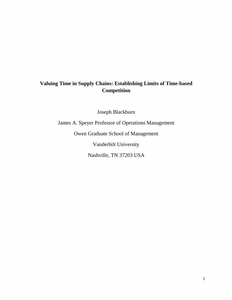
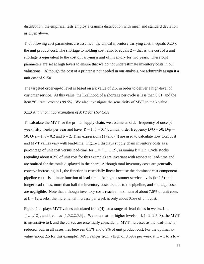
and MVT values vary with lead-time. Figure 1 displays supply chain inventory costs as a

percentage of unit cost versus lead-time for L = {1,…,12}, assuming k = 2.5. Cycle stocks

(equaling about 0.2% of unit cost for this example) are invariant with respect to lead-time and

are omitted for the totals displayed in the chart. Although total inventory costs are generally

concave increasing in L, the function is essentially linear because the dominant cost component--

pipeline cost-- is a linear function of lead-time. At high customer service levels (k=2.5) and

longer lead-times, more than half the inventory costs are due to the pipeline, and shortage costs

are negligible. Note that although inventory costs reach a maximum of about 7.5% of unit costs

at L = 12 weeks, the incremental increase per week is only about 0.5% of unit cost.

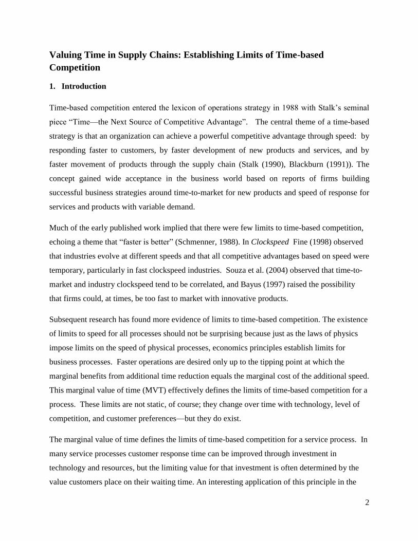
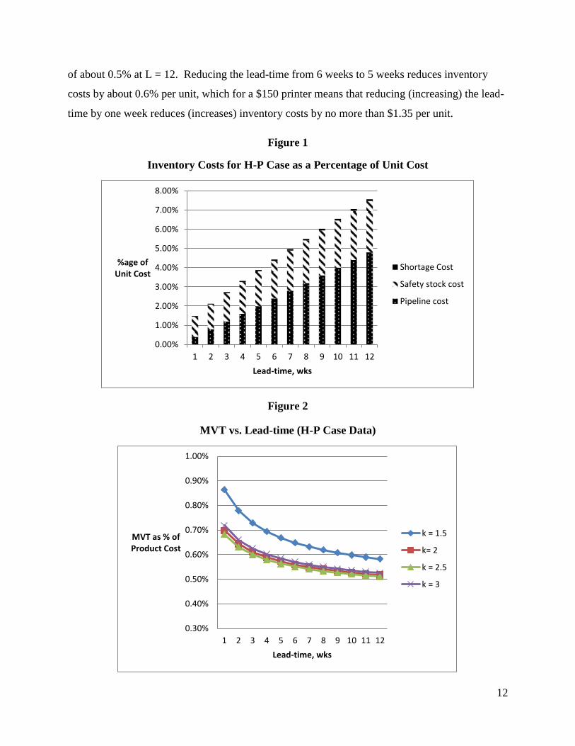
Figure 2 displays MVT values calculated from (4) for a range of lead-times in weeks, L =

{1,…,12}, and k values {1.5,2,2.5,3}. We note that for higher levels of k (= 2, 2.5, 3), the MVT

is insensitive to k and the curves are essentially coincident. MVT increases as the lead-time is

reduced, but, in all cases, lies between 0.5% and 0.9% of unit product cost. For the optimal k-

value (about 2.5 for this example), MVT ranges from a high of 0.69% per week at L = 1 to a low

12

of about 0.5% at L = 12. Reducing the lead-time from 6 weeks to 5 weeks reduces inventory

costs by about 0.6% per unit, which for a $150 printer means that reducing (increasing) the lead-

time by one week reduces (increases) inventory costs by no more than $1.35 per unit.

Figure 1

Inventory Costs for H-P Case as a Percentage of Unit Cost

Figure 2

MVT vs. Lead-time (H-P Case Data)

0.00%

1.00%

2.00%

3.00%

4.00%

5.00%

6.00%

7.00%

8.00%

1 2 3 4 5 6 7 8 9 10 11 12

%age of Unit Cost

Lead-time, wks

Shortage Cost

Safety stock cost

Pipeline cost

0.30%

0.40%

0.50%

0.60%

0.70%

0.80%

0.90%

1.00%

1 2 3 4 5 6 7 8 9 10 11 12

MVT as % of Product Cost

Lead-time, wks

k = 1.5

k= 2

k = 2.5

k = 3

13

3.2.4 Testing the MVT Approximation

To test the accuracy of the analytical approximation for the H-P example, we conducted

extensive simulations of the supply chain with the same parameters as described above, collected

inventory costs, and from those data developed estimates for the MVT at different levels of k and

L. For each set of parameter values, we ran a long initialization period and then took ten samples

of 2500 weeks (or about 50 years) of simulated operation; weekly demands were drawn from a

gamma distribution with mean 3650 and standard deviation 2700. Recall that the analytical

estimates for MVT (Figure 2) are based on a normal distribution, so some deviation between the

simulation and the analytical results is expected. Tyworth and O’Neill (1997) tested the use of

the normal approximation for a variety of demand distributions and found it to be robust with

respect to inventory costs.

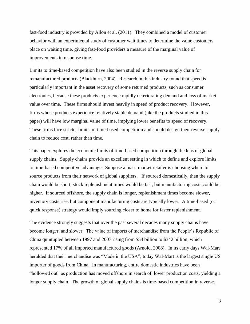
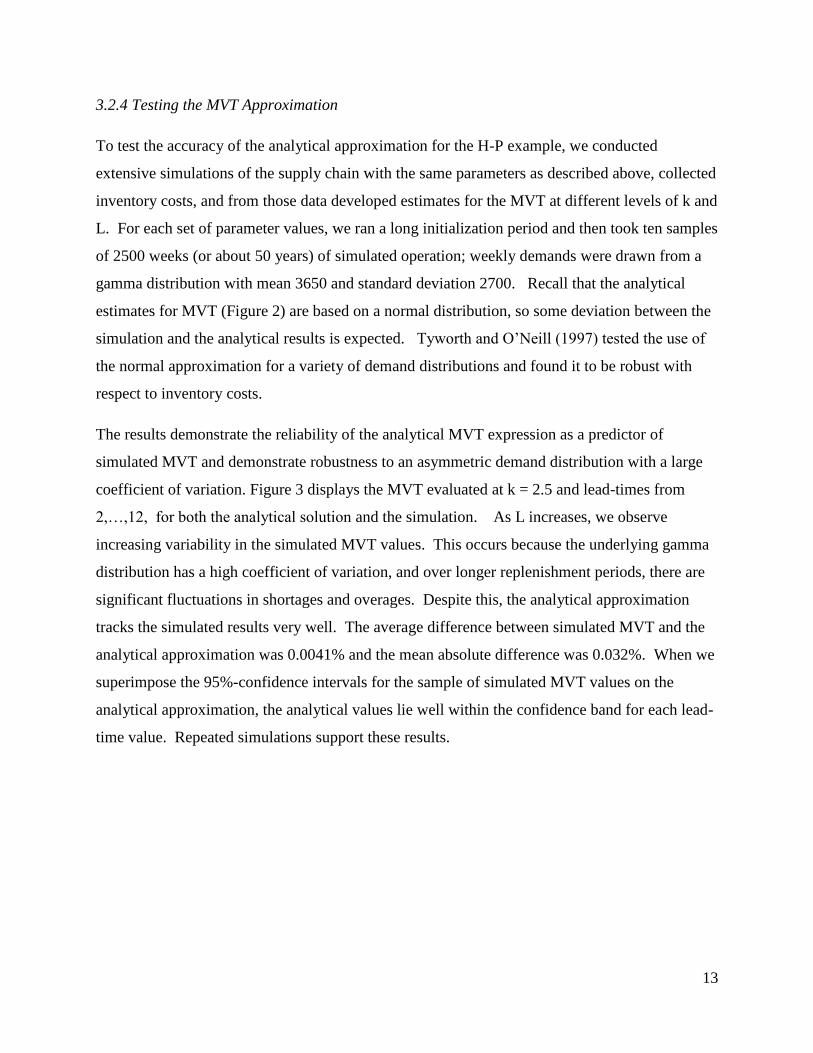
The results demonstrate the reliability of the analytical MVT expression as a predictor of

simulated MVT and demonstrate robustness to an asymmetric demand distribution with a large

coefficient of variation. Figure 3 displays the MVT evaluated at k = 2.5 and lead-times from

2,…,12, for both the analytical solution and the simulation. As L increases, we observe

increasing variability in the simulated MVT values. This occurs because the underlying gamma

distribution has a high coefficient of variation, and over longer replenishment periods, there are

significant fluctuations in shortages and overages. Despite this, the analytical approximation

tracks the simulated results very well. The average difference between simulated MVT and the

analytical approximation was 0.0041% and the mean absolute difference was 0.032%. When we

superimpose the 95%-confidence intervals for the sample of simulated MVT values on the

analytical approximation, the analytical values lie well within the confidence band for each lead-

time value. Repeated simulations support these results.

14

Figure 3

MVT Simulation vs. Analytical Model

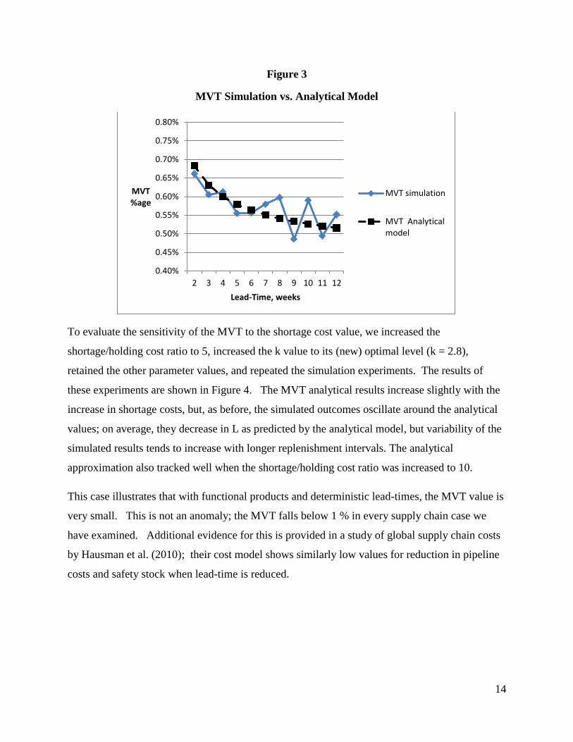
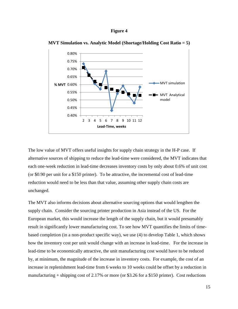
To evaluate the sensitivity of the MVT to the shortage cost value, we increased the

shortage/holding cost ratio to 5, increased the k value to its (new) optimal level (k = 2.8),

retained the other parameter values, and repeated the simulation experiments. The results of

these experiments are shown in Figure 4. The MVT analytical results increase slightly with the

increase in shortage costs, but, as before, the simulated outcomes oscillate around the analytical

values; on average, they decrease in L as predicted by the analytical model, but variability of the

simulated results tends to increase with longer replenishment intervals. The analytical

approximation also tracked well when the shortage/holding cost ratio was increased to 10.

This case illustrates that with functional products and deterministic lead-times, the MVT value is

very small. This is not an anomaly; the MVT falls below 1 % in every supply chain case we

have examined. Additional evidence for this is provided in a study of global supply chain costs

by Hausman et al. (2010); their cost model shows similarly low values for reduction in pipeline

costs and safety stock when lead-time is reduced.

0.40%

0.45%

0.50%

0.55%

0.60%

0.65%

0.70%

0.75%

0.80%

2 3 4 5 6 7 8 9 10 11 12

MVT %age

Lead-Time, weeks

MVT simulation

MVT Analyticalmodel

15

Figure 4

MVT Simulation vs. Analytic Model (Shortage/Holding Cost Ratio = 5)

The low value of MVT offers useful insights for supply chain strategy in the H-P case. If

alternative sources of shipping to reduce the lead-time were considered, the MVT indicates that

each one-week reduction in lead-time decreases inventory costs by only about 0.6% of unit cost

(or $0.90 per unit for a $150 printer). To be attractive, the incremental cost of lead-time

reduction would need to be less than that value, assuming other supply chain costs are

unchanged.

The MVT also informs decisions about alternative sourcing options that would lengthen the

supply chain. Consider the sourcing printer production in Asia instead of the US. For the

European market, this would increase the length of the supply chain, but it would presumably

result in significantly lower manufacturing cost. To see how MVT quantifies the limits of time-

based completion (in a non-product specific way), we use (4) to develop Table 1, which shows

how the inventory cost per unit would change with an increase in lead-time. For the increase in

lead-time to be economically attractive, the unit manufacturing cost would have to be reduced

by, at minimum, the magnitude of the increase in inventory costs. For example, the cost of an

increase in replenishment lead-time from 6 weeks to 10 weeks could be offset by a reduction in

manufacturing + shipping cost of 2.17% or more (or $3.26 for a $150 printer). Cost reductions

0.40%

0.45%

0.50%

0.55%

0.60%

0.65%

0.70%

0.75%

0.80%

2 3 4 5 6 7 8 9 10 11 12

% MVT

Lead-Time, weeks

MVT simulation

MVT Analyticalmodel

16

of this size, and more, are often achievable by switching to offshore sourcing from a lower labor

cost country.

Table 1

Increase in Inventory Cost for Longer Lead-times

Lead-Time

(in Weeks)

% Increase in

Inventory Cost Per Unit

$ increase in

Cost Per Unit

6 0.00% $0.00

7 0.56% $0.83

8 1.11% $1.67

9 1.65% $2.48

10 2.17% $3.26

11 2.69% $4.04

3.3 The Marginal Value of Time for Variable Lead-times

In this section we extend the MVT model to include supply chains with stochastic replenishment

times. This requires an additional assumption about how lead-time variability changes with lead-

time. Fang et al. (2011) examine lead-time variability in a study of for orders placed by a major

international steel producer with their 22 suppliers and found strong positive correlation between

lead-time and lead-time variability. Statistical principles would also support such a relationship:

if lead-time were assumed to be the sum of L independent, identically distributed random

variables, then lead-time variance would be a linear, increasing function of L.

We develop MVT approximations under two different assumptions about the relationship

between mean lead-time L and lead-time variability (1) variance of leadtime is linear in L,

i.e.

, where is the variance of a one-period replenishment time; (2) standard

deviation of leadtime is linear in L, that is, . Both assumptions imply a strong positive

correlation between lead-time and lead-time variability. We include the second assumption in

order to investigate the effects on cost in situations for which lead-time variability increases at

rate that is quadratic, rather than linear, in L. The detailed development of the MVT analytical

models for both fixed-review and continuous-review policies are provided in Appendix B.

17

In this paper we will report on empirical tests of the MVT approximation for a general fixed-

review period (Q,R,k) policy when condition (1) applies—that is, the variance of lead-time is

assumed to be linear in L. From Appendix B, equation (B.3), we have

( )

( )

[

[ (

) ( )] [

√[( ) ]

]

( ⁄ )(

)(

) ( ( ) ( ))

]

(5)

Expression (5) is similar in structure to the MVT approximation for deterministic lead-times,

expression (4); lead-time variability increases all the terms in the MVT expression except for the

pipeline inventory term,

( ) .

3.3.1 Example: Calculating the Analytical MVT in an Electrical Equipment Supply Chain

We have investigated the effect of variable lead-time on the supply chain MVT in several

applications and report here on one illustrative example: a US manufacturer of electrical

equipment who sources components from domestic suppliers and also from Mexico and Asia.

In this example we focus on one of their major outsourced components—ballasts. Ballasts are

ordered from a manufacturer in Asia and held at the US manufacturing facility for the assembly

of electrical lighting products. The total manufacturing plus shipping cost averages about

$15/unit (although the analysis is not dependent on the cost of a unit).

Inventory is managed by the firm as follows: a periodic-review inventory policy is followed in

which the inventory position is reviewed at the US manufacturing facility every 20 days (or

every 4 weeks based on a 5-day week) and a replenishment order is issued to the Asian

manufacturer. Analysis of order and shipping data for a two-year period indicated that the lead-

time for replenishment from the supplier averaged about 40 days (or 8 weeks), and the

coefficient of variation of lead-time was 0.2.

Demand for the component is based on scheduled manufacturing requirements, which averaged

about 90 units per day. However, demand is highly variable; it equaled zero on about 60% of the

days. The coefficient of variation of daily demand equaled 1.35. Because the MVT

approximation assumes normally distributed demand and actual daily demand is not normally

18

distributed (the modal demand value is zero), this example provides another test of the

robustness of the approximation to differences in demand distributions.

Analytical approximations of MVT were obtained using the fixed-review period model

(expression (5). We assumed a fixed review period identical to that used by the firm (R = 4

weeks), and, given that the firm orders ballasts 10-13 times per year, we assumed a worst-case

estimate of the order frequency (D/Q = 13). The annual inventory carrying cost percentage was

identical to that used by the firm (i = 0.15), and a penalty cost/holding cost ratio of 2 was

selected to reflect high customer service requirements. Lead-time variance was assumed to be

linear in L, with a coefficient of variation of 0.2 at eight weeks in order to equal that observed in

the supply chain

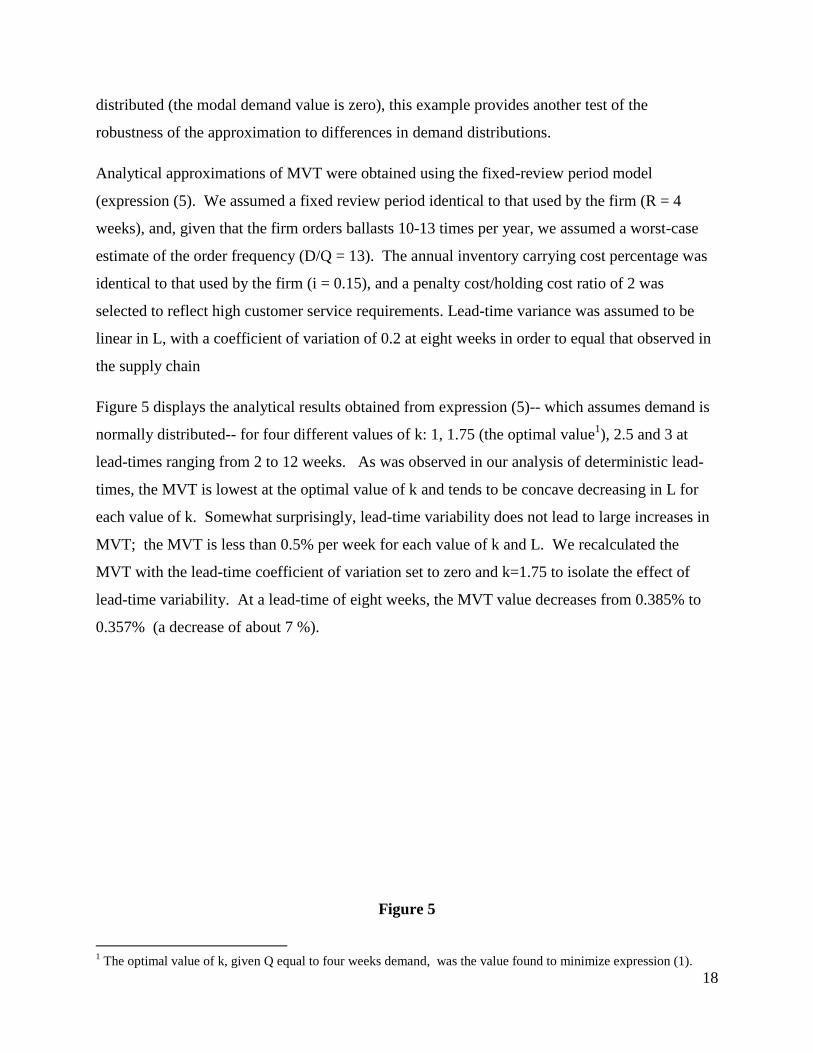
Figure 5 displays the analytical results obtained from expression (5)-- which assumes demand is

normally distributed-- for four different values of k: 1, 1.75 (the optimal value1), 2.5 and 3 at

lead-times ranging from 2 to 12 weeks. As was observed in our analysis of deterministic lead-

times, the MVT is lowest at the optimal value of k and tends to be concave decreasing in L for

each value of k. Somewhat surprisingly, lead-time variability does not lead to large increases in

MVT; the MVT is less than 0.5% per week for each value of k and L. We recalculated the

MVT with the lead-time coefficient of variation set to zero and k=1.75 to isolate the effect of

lead-time variability. At a lead-time of eight weeks, the MVT value decreases from 0.385% to

0.357% (a decrease of about 7 %).

Figure 5

1 The optimal value of k, given Q equal to four weeks demand, was the value found to minimize expression (1).

19

MVT vs. Lead-Time (Electrical Equipment Manufacturer)

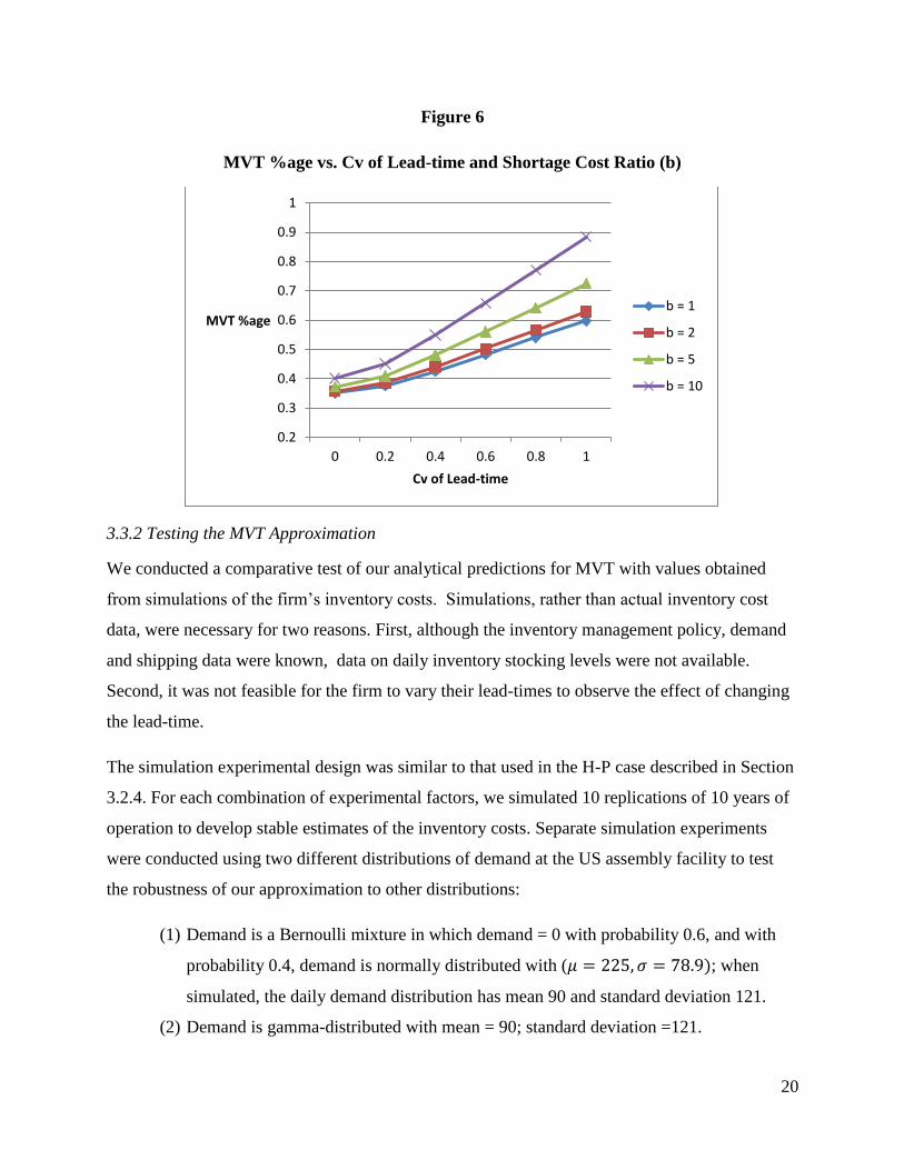
We conducted an additional test of the sensitivity of MVT to both the shortage cost ratio and

lead-time coefficient of variation (Cv), assuming a lead-time of eight weeks (and k = 1.75).

These results are displayed in Figure 6, in which MVT is plotted as a function of lead-time Cv

for shortage costs ratios ranging from 1 to 10. As expected, the MVT increases in both Cv and

the shortage cost ratio; however, all the MVT values lie below 0.9% of unit cost per week and

only exceeds 0.8% at Cv = 1, b = 10. These results imply that MVT remains below 1% per week

even for highly-variable lead-times and high shortage cost values.

0.35

0.37

0.39

0.41

0.43

0.45

0.47

0.49

0.51

0.53

0.55

2 3 4 5 6 7 8 9 10 11 12

MVT %

Lead-time, weeks

k=1

k=1.75

k=2.5

k=3

20

Figure 6

MVT %age vs. Cv of Lead-time and Shortage Cost Ratio (b)

3.3.2 Testing the MVT Approximation

We conducted a comparative test of our analytical predictions for MVT with values obtained

from simulations of the firm’s inventory costs. Simulations, rather than actual inventory cost

data, were necessary for two reasons. First, although the inventory management policy, demand

and shipping data were known, data on daily inventory stocking levels were not available.

Second, it was not feasible for the firm to vary their lead-times to observe the effect of changing

the lead-time.

The simulation experimental design was similar to that used in the H-P case described in Section

3.2.4. For each combination of experimental factors, we simulated 10 replications of 10 years of

operation to develop stable estimates of the inventory costs. Separate simulation experiments

were conducted using two different distributions of demand at the US assembly facility to test

the robustness of our approximation to other distributions:

(1) Demand is a Bernoulli mixture in which demand = 0 with probability 0.6, and with

probability 0.4, demand is normally distributed with ( ); when

simulated, the daily demand distribution has mean 90 and standard deviation 121.

(2) Demand is gamma-distributed with mean = 90; standard deviation =121.

0.2

0.3

0.4

0.5

0.6

0.7

0.8

0.9

1

0 0.2 0.4 0.6 0.8 1

MVT %age

Cv of Lead-time

b = 1

b = 2

b = 5

b = 10

21

We first describe the results of simulations based on the Bernoulli mixture distribution of zero

and normally-distributed values; this distribution was a good fit for the observed demand. Cost

parameters and ordering policies were identical to those used to obtain the MVT analytical

approximations. In addition to the difference in demand distributions, there is another potential

source of difference between the analytical results and the simulation: it is possible in the

simulation to have order crossover (which tends to reduce the expected lead-time). The analytical

model assumes normally distributed demand and no order crossover. Bischak et al. (2011)

reported on extensive experimentation of the effects of order crossover in supply chains with

variable lead-times. With long review periods of four weeks, as in our case, the likelihood of

significant order crossover is low, both in practice and in a simulation.

The results using an optimal k value of 1.75 and an eight-week lead-time in the simulations are

shown in Figure 7, where have superimposed the analytical MVT values for comparison. The

simulated MVT values oscillate about the analytic values as we previously observed in the

deterministic lead-time tests (Section 3.2.4), but the addition of lead-time variability increases

the magnitude of the oscillations. The average percentage deviation between analytic and

simulated values equals 0.007% (average absolute percentage deviation equals 0.047%), and all

the MVT analytical values fell within the 95% confidence interval for the simulated mean

values. The analytical approximation is a highly-reliable predictor.

22

Figure 7

MVT Analytic vs. Simulation (Bernoulli Mixed Demand Distribution)

Simulations conducted with gamma-distributed demand are displayed in Figure 8 and yielded

similar results. Due to extreme values in gamma-distributed demand, the simulated MVT results

exhibit higher levels of variability than observed with the Bernoulli-mixture demand. However,

the average deviation between simulated and analytic values equals 0.008%, not significantly

higher. And the analytical values all lie within the 95% confidence intervals for the simulated

means. These results imply that, even at relatively high levels of demand variability, the normal

approximation is robust.

Although not included in the paper, we have also conducted similar experiments under the

assumption that the lead-time standard deviation is linear in L, with similar results: the

analytical model is an excellent predictor of simulated MVT results, and MVT values falls

within a similar range.

0.2

0.25

0.3

0.35

0.4

0.45

0.5

2 3 4 5 6 7 8 9 10 11 12

MVT %age

Lead-time, weeks

MVT Simulation

MVT Analytical

23

Figure 8

MVT Analytic vs. Simulation (Gamma-distributed Demand)

What insights does the marginal value of time offer for supply chain and sourcing strategy for

this electrical equipment manufacturer? Using their manufacturing facilities in Mexico, they

could adopt a time-based strategy with faster replenishment times by sourcing there rather than

Asia, reducing their lead-time by up to three weeks. However, at their current lead-time values,

a change in lead-time of one week would change their inventory costs (including pipeline) by

about 0.4% of unit costs, and a three-week reduction would yield incremental savings in

inventory costs that are no more than 1.5% of unit cost. Manufacturing costs would increase due

to higher labor and material costs, and shipping costs would decrease. Assuming other costs of

managing the supply chain do not change, the increase in manufacturing cost would outweigh

the projected reduction in inventory costs, unless this cost, net of shipping, is less than 1.5%.

The low value of MVT clearly imposes limits on time-based competition because the rewards in

(inventory) cost reduction gained by faster replenishment from Mexico are meager. Even with

variability in lead-time, changes in the lead-time have a very small effect on inventory costs,

when measured as a percentage of unit costs. This reinforces the recommendation by Fisher

0

0.1

0.2

0.3

0.4

0.5

0.6

2 3 4 5 6 7 8 9 10 11

MVT %

Lead-Time, Weeks

MVT Sim

MVT Analytical

24

(1997) that the supply chain for functional products should be designed more for cost efficiency

than speed.

4. Conclusions

The utility of the MVT analytic expression derives from its broad generality and computational

simplicity. The empirical tests show that it accurately estimates the effect on inventory costs of a

change in the lead-time for any functional product, under all commonly-used reorder-point

inventory policies, even with lead-time variability. It is robust to the assumption of a normal

distribution under all but the most extreme, or contrived, conditions.

Unlike most models of supply chain inventory management which assume, or prescribe, optimal

behavior, our MVT model does not. This is a strength that greatly expands the applicability of

the model because most inventories in practice are managed sub-optimality. Our approximations

apply to, but are not restricted by, a requirement of optimality, and thus are free of some of the

assumptions that limit traditional models.

The simple transformation of the metric in our model from total cost to cost as a percentage of

unit product cost significantly increases the generality of the results and offers new insights into

the relationship between supply chain lead-time and inventory costs. When the marginal value

of time is computed in terms of total costs, the results are obscured by the unit cost effect: that is,

marginal values look large for expensive products and small for low-cost products. But when

viewed as a percentage of unit product cost, we find that the marginal values for all products fall

within a narrow band, yielding an important, all-inclusive result. The main qualitative result of

this paper is that inventory-related costs, when measured as a percentage of unit cost, are

relatively insensitive to changes in the lead-time. Quantitatively, our examples show that the

MVT tends to fall within a range of from 0.4% to 0.8% of unit product cost per week of lead-

time change.

The low marginal value of time provides a partial explanation for the surge in outsourcing and

the longer supply chains that have been observed over the past few decades. Offshore sources

have long offered lower manufacturing costs, and once these sources attained quality levels

similar to domestic US manufacturing, there were few economic barriers to lengthening the

supply chain to tap those sources. Inventory costs are not an effective bulwark against the

25

offshoring of functional products, and the low marginal cost of increases in time has effectively

limited time-based competition.

This paper has focused only on the effects of lead-time changes on inventory costs in supply

chains, and there are, of course, other costs associated with global supply chains. As offshore

supply chains become longer and more complex, costs associated with coordination, disruption

risk, and obsolescence tend to rise. And to the extent that these costs vary with changes in lead-

time, they also strongly influence sourcing decisions. For innovative or fashion-oriented

products with short life cycles, our results about the effect of lead-time changes on inventory

costs would still hold. However, costs of obsolescence and markdowns would become much

more important, even dominant, and would raise the value of time-based response. An

investigation into the value of time, scaled to unit product cost, in the supply-chain for

innovative products would be an interesting subject for future research.

References

Allon, G., Federgruen, A., Pierson, M., 2011. How much is a reduction of your customers’ wait

worth? An empirical study of the fast-food drive-thru industry based on structural estimation

methods. M&SOM-Manuf. Serv. Op. 13, 4, 489-507.

Arnold, B. 2008. How changes in the value of the Chinese currency affect US imports.

Congressional Budget Office paper. http//ww.cbo.gob/ftpdocs/95xx/doc9506/ChinaTOC.2.1.htm

Bayus, B.S., Jain, S., Rao, A., 1997. Too little, too early: Introduction timing and new product

performance in the personal digital assistant industry. J. Marketing. Res. 34, 50-63.

Bischak, D., Robb, D., Silver, E.A., J.D. Blackburn, J.D., 2011. Analysis and management of

periodic review, order-up-to-level inventory systems with order crossover. Working Paper Owen

Graduate School of Management, Vanderbilt University.

Blackburn, J. (ed.), 1991. Time-Based Competition: The Next Battleground in American

Manufacturing. BusinessOne Irwin, Homewood, IL.

Blackburn, J.D., 2001. Limits of time-based competition: strategic sourcing decisions in make-

to-stock manufacturing, Working Paper, Owen Graduate School of Management, Vanderbilt

University, Nashville, TN.

26

Blackburn, J.D., Guide, Jr., V.D.R., Souza, G.C., Van Wassenhove, L.N., 2004. Reverse supply

chains for commercial returns. 46, 2, 6-22.

Callioni, G., de Montros, X., Slagmulder, R., Van Wassenhove, L.N., Wright, L., 2005.

Inventory-driven costs. Harvard Bus. Rev. 83, 3, 135-141.

Caro, F., Martinez-de-Albeniz, V., 2010. The impact of quick reponse in inventory-based

competition. M&SOM-Manuf. Serv. Op. 12, 3, 409-429.

Fang, X., Zhang, C., Robb, D.J., Blackburn, J.D., 2011. Decision support for lead time and

demand variability reduction. Working Paper Owen Graduate School of Management.

Vanderbilt University.

Fisher, M.L., Raman, A., 1996. Reducing the cost of demand uncertainty through accurate

response to early sales. Oper. Res., 44, 11, 87-99.

Fisher, M.L., 1997. What is the right supply chain for your product? Harvard Bus. Rev. 75, 2,

105-116.

Fine, C.H. 1998. Clockspeed: Winning Industry Control in the Age of Temporary Advantage.

Perseus Books, Reading, MA.

Hadley, G., Whitin, T.M., 1963. Analysis of Inventory Systems. Prentice-Hall, Englewood

Cliffs, NJ.

Handfield, R.B., 1995. Re-engineering for Time-based Competition: Benchmarks and Best

Practices for Production R & D, and Purchasing. Quorum Books, Westport, CT.

Hausman, W.H., Lee, H.L., Napier, G.R.E., Thompson, A., Zheng, Y., 2010. A process analysis

of global trade management: an inductive approach. Supply Chain Manag. 46, 2, 5-29.

Hill, A., Khosla, I., 1992. Models for optimal lead time reduction, Prod. Oper. Manag. 1:2, 185-

197.

Holweg, M., Reichhart, A., Hong, E., 2011. On risk and cost in global sourcing. Int. J. Prod.

Econ. 131, 333-341.

27

Iyer, A.V., Bergen, M.E., 1997. Quick response in manufacturer-retailer channels. Manage. Sci.,

43, 4, 559-570.

Kopczak, L., Lee, H. 2004. Hewlett-Packard Company: DeskJet Printer Supply Chain (A).

Stanford Graduate School of Business Case GS-3A.

Lederer, P., Li, L., 1997. Pricing, production, scheduling, and delivery-time competition. Oper.

Res. 45:3, 407-420.

Lowson, R.H., 2002. Assessing the operational cost of offshore sourcing strategies. Int. J. Prod.

Man. 13, 2, 79-89.

Porteus, E.L., 1985. Investing in reduced setups in the EOQ model. Manage. Sci. 31, 998-1010.

Schmenner, R.W. 1988. The merit of making things fast. Sloan Mgt. Rvw. Fall, 1998, 11-17.

Shang,W., Liu, L., 2011. Promised delivery time and capacity games in time-based competition.

Manage. Sci. 57,3, 599-610.

So, K.C., 2000. Price and time competition for service delivery. M&SOM- Manuf. Serv. Op. 2,

4, 392-409.

Souza, G.C., Bayus, B.L., Wagner, H.M., 2004. New-product strategy and industry clockspeed.

Manage. Sci. 50, 4, 537-549.

Stalk, G., Jr., 1988. Time—the next source of competitive advantage. Harvard Bus. Rev. 66, 4,

41-51.

Stalk, G., Jr., Hout, T., 1990. Competing Against Time. The Free Press, New York.

Suri, R., 1998. Quick Response Manufacturing: A Companywide Approach to Reducing Lead

Times. Productivity Press, Portland, OR.

Tyworth, J.E., O’Neill, L., 1997. Robustness of the normal approximation of lead-time demand

in a distribution setting. Nav. Res. Logist. Q. 44, 165-186.

Zipkin, P.H., 2000. Foundations of Inventory Management. McGraw-Hill, New York.

28

Appendix A: Approximations for the Marginal Value of Time under Deterministic Lead-Times

We first develop approximations to MVT for different reorder-point inventory policies under the

assumption of deterministic lead-times. Using (3), and substituting

( ) ( ) [ ( ) (

)] from Zipkin (2000), we have

( )

(

) ⌊ (

) ( ( ⁄ ) ( )) ( ) (

) ( ( ) (

))

(

) (

)

⌋ (A.1)

(A.1) is an exact expression of MVT for continuous-review policies under normally-distributed

demand and deterministic lead-times. We obtain a simpler approximation by omitting the two

small negative terms in (A.1) that adjust the expected backorder term in the event that an

incoming order is insufficient to fill all outstanding backorders. The two negative terms have

insignificant values in most practical cases and, by omitting them, we ensure that the MVT value

obtained is a very tight upper bound on the exact value. Then, substituting √ for

deterministic lead-times, we have the following approximation for continuous-review policies

with backlogged demands

( ) (

( ⁄ )) ⌊

√ ( ( ⁄ ) ( ))

( ⁄ )( ( ))⌋ (A.2)

Expression (A.2) may be modified for the lost-sales case by redefining b as the ratio of the cost

of a lost sale, , to the annual unit holding cost and dropping the last term in (A.2), which

adjusts inventory for expected backorders.

Fixed-review period (Q,R,k,L) policies:

If inventory is observed every R periods, then the pipeline inventory is identical to the

continuous-review case ( ), but √ because safety stock is based on L+R standard

deviations of demand, and, from (A.2) and (k) =(

) [ ( ) ( ))] , we have

29

( ) (

( ⁄ )) ⌊

√ ( ( ⁄ ) ( ))

( ⁄ )( ( ) ( ))

⌋ (A.3)

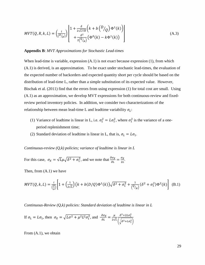
Appendix B: MVT Approximations for Stochastic Lead-times

When lead-time is variable, expression (A.1) is not exact because expression (1), from which

(A.1) is derived, is an approximation. To be exact under stochastic lead-times, the evaluation of

the expected number of backorders and expected quantity short per cycle should be based on the

distribution of lead-time L, rather than a simple substitution of its expected value. However,

Bischak et al. (2011) find that the errors from using expression (1) for total cost are small. Using

(A.1) as an approximation, we develop MVT expressions for both continuous-review and fixed-

review period inventory policies. In addition, we consider two characterizations of the

relationship between mean lead-time L and leadtime variability

(1) Variance of leadtime is linear in L, i.e.

, where is the variance of a one-

period replenishment time;

(2) Standard deviation of leadtime is linear in L, that is, .

Continuous-review (Q,k) policies; variance of leadtime is linear in L

For this case, √ √ , and we note that

.

Then, from (A.1) we have

( )

(

)[ (

√ ) ( ( ) ( ))√

( ⁄ )(

) ( )] (B.1)

Continuous-Review (Q,k) policies: Standard deviation of leadtime is linear in L

If , then √ , and

√

(√ )

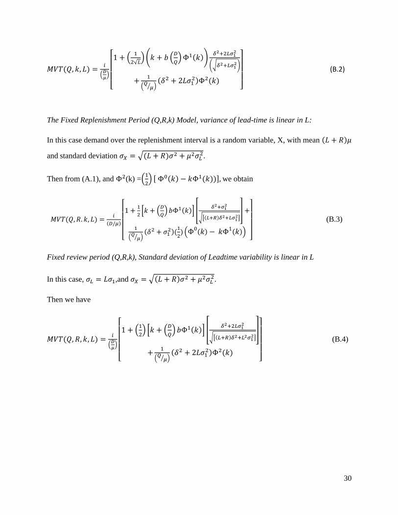
From (A.1), we obtain

30

( )

(

)

[ (

√ ) ( (

) ( ))

(√ )

( ⁄ )(

) ( )]

(B.2)

The Fixed Replenishment Period (Q,R,k) Model, variance of lead-time is linear in L:

In this case demand over the replenishment interval is a random variable, X, with mean ( )

and standard deviation √( ) .

Then from (A.1), and (k) =(

) [ ( ) ( ))] we obtain

( )

( )

[

[ (

) ( )] [

√[( ) ]

]

( ⁄ )(

)(

) ( ( ) ( ))

]

(B.3)

Fixed review period (Q,R,k), Standard deviation of Leadtime variability is linear in L

In this case, ,and √( )

.

Then we have

( )

(

)

[ (

) [ (

) ( )] [

√[( ) ]]

( ⁄ )(

) ( )]

(B.4)