Embed Size (px)
Citation preview

Valuing Real Options using Implied Binomial Trees and Commodity Futures Options
Tom Arnold The Robins School of Business
Department of Finance 1 Gateway Road
University of Richmond Richmond, VA 23173
O: 804-287-6399 F: 804-289-8878
Timothy Falcon Crack Dept. Finance and Quant. Analysis,
Otago University, PO Box 56, Dunedin, New Zealand.
Tel: +64(0)3-479-8310 Fax: +64(0)3-479-8193
Adam Schwartz Washington and Lee University
Williams School of Commerce, Economics, and Politics Lexington, VA 24450
April 11, 2006
We thank David Alexander and an anonymous referee for comments. Any errors are ours.

Valuing Real Options using Implied Binomial Trees and Commodity Futures Options
Abstract:
A real option on a commodity is valued using an implied binomial tree (IBT) calibrated
using commodity futures options prices. Estimating an IBT in the absence of spot options
(the norm for commodities) allows real option models to be calibrated for the first time to
market-implied probability distributions for commodity prices. Also, the existence of
long-dated futures options means that good volatility estimates may now be incorporated
into capital budgeting evaluations of real options projects with long planning horizons.
An example is given using gold futures options and a real option to extract gold from a
mine. We include a unique out-of-sample test that shows how IBT option pricing errors
evolve on sub-trees emanating from future levels of the underlying.
2
I. Introduction We show how to use implied binomial trees (IBTs) for the valuation of real
options where the underlying asset that drives the value of the real option is a physical
commodity for which futures options exist but for which spot options do not exist (e.g.,
gold, silver, platinum, oil, wheat). The absence of listed spot options is the norm for
commodities, and this means that until now it has not been possible to calibrate an IBT of
commodity prices using traded options. By showing how to fit an IBT to commodity
prices without using spot options, it is now possible to estimate binomial option pricing
models that completely relax the traditional binomial tree’s rigid assumption that
commodity prices be distributed lognormal.1 In addition, the existence of long-dated
futures options means that good volatility estimates may now be incorporated into capital
budgeting evaluations of real options projects with long planning horizons.2 An example
is given using a gold mine, but the technique also applies to non-investment commodities.
We also include a unique out-of-sample test using long-dated options that shows how
option pricing errors evolve if you hold fixed the estimated tree and look at conditional
pricing on sub-trees emanating from future levels of the underlying.
II. Implied Binomial Trees
Implied binomial trees infer consensus market views on future risk-neutral
distributions for the underlying asset. By calibrating the tree to the market prices of
traded options, skewness and kurtosis within the distribution of returns to the underlying
asset are incorporated into the tree and can be used to price other, possibly non-traded,
options based on the tree. Some of these higher moments implicitly account for jump
3

probabilities, although they are not modelled explicitly as such. The IBT produces these
benefits with much less quantitative machinery than many other analytic techniques.
The three best-known implied binomial tree techniques are due to Derman and
Kani (1994), Rubinstein (1994), and Jackwerth (1997). Each technique has different
strengths and weaknesses. The core differences between the techniques that are relevant
for the present paper are:
• Jackwerth’s 1997 generalized implied binomial tree (J-GIBT) is calibrated using
American-style options of different maturities, whereas Rubinstein’s 1994 implied
binomial tree (R-IBT) is calibrated using only European-style options of a single
maturity.
• The R-IBT assumes binomial path independence (BPI). That is, all paths leading
to a single node have the same probability of being traversed (Chriss, 1997,
p417). The J-GIBT and Derman-Kani trees do not assume BPI. The R-IBT is thus
quite inflexible with respect to the internal probability structure of the binomial
tree. The J-GIBT and Derman-Kani trees, however, allow more flexibility so that
intermediate maturity and American-style options may be priced.
• The Derman-Kani technique can be difficult to implement and unstable because
of bad probabilities, but the R-IBT (and therefore the J-GIBT) techniques do not
suffer from these problems (Chriss, 1997, p431).
We choose to use the J-GIBT because of its ease of estimation, flexibility, and stability.
4

III. Literature on Pricing Commodity Futures Options and Commodity Futures
The most important factors affecting commodity prices are general shifts in the
cost of producing the commodity and general shifts in the demand for the commodity
(Black, 1976, p. 174). Interest rates and storage costs are important to a lesser extent.
Changes in demand and supply are reflected in the convenience yield.
Let δ denote the average continuously-compounded net convenience yield
(consumption benefit less storage costs) for a commodity from time-t (now) to time-T
(expiration of a futures contract on the commodity). See the timeline in Figure 1. Let r
denote the average continuously-compounded riskless interest rate over the same period.
Let S denote the spot price of the commodity at time-t. Then a fair price at time-t for
future delivery of the commodity at time-T is given by ( )( )tTrteSTtF −−= δ),( . In the case of
a physical commodity, δ is typically not directly observable, but it may be deduced as the
only non observable in the equation.
The consumption benefit is the benefit of direct access to a commodity. The
owner of the commodity (possibly the short position on a futures contract) receives the
consumption benefit, but the owner of the futures on the same commodity does not
receive the consumption benefit. In the case of a financial security, there is no storage
cost and δ is just the continuous dividend yield. Indeed, Carmona and Ludkovski (2003)
consider the convenience yield as a correction to the drift for the spot process that is in
essence a dividend. In the case of gold and silver and other investment commodities held
by many people for investment motives the marginal trader is not holding them for
consumption. So, the consumption benefit is zero and the net convenience yield reduces
just to the storage costs (Hull, 2000, pp72–73).
5

In the case of consumption commodities (where the marginal trader holds the
commodity in inventory for use in production), the convenience yield issue becomes
much more involved.
The interaction of spot, futures, and convenience yield is complicated. Gibson and
Schwartz (1990) present an analytical two-factor model for oil prices (the two factors are
randomness in the price of oil and in the instantaneous convenience yield). The authors
estimate the market price of convenience yield risk and find it to be negative (suggesting
that it pays to bear convenience yield risk). A forward curve of convenience yields is
implied by forward contracts of different maturity. The curve displays considerable mean
reversion in convenience yields—driven by oil inventories, shortages, fears of Middle
East wars etc.
Miltersen and Schwartz (1998) present analytical models for pricing commodity
futures options. Their models allow for stochastic convenience yields and stochastic
interest rates and are a closed-from generalization of the Black-Scholes formula. Hilliard
and Reis (1998) attack a similar problem to Miltersen and Schwartz but their model
allows for jump diffusions in commodity prices and for excess (positive or negative)
skewness in the distribution of the commodity price. The Hilliard-Reis model also allows
for a no-arbitrage term structure of convenience yields and is a three-factor model (spot,
convenience yields, and jumps or alternatively spot, convenience yields and interest
rates).
Hilliard and Reis (1998) present a real option valuation problem (the price of one
barrel of oil) using their forward pricing formula. They provide a good discussion of why
assuming that an instantaneous convenience yield remaining at its current level rather
6

than reverting to a long run mean can bias pricing (Hilliard and Reis, 1998, pp. 78–79).
Further, a positive correlation between the spot price process and the spot convenience
yield generates mean reverting behavior to the spot commodity price (Miltersen and
Schwartz, 1998, p. 34).
IV. Properties of the Method
To implement the method, choose a commodity and a futures contract on that
commodity maturing at time T. Assume that the net convenience yield δ and the riskless
interest rate r between time-t and time-T are non-stochastic and equal to the convenience
yield implied by the futures contract and the riskless rate implied by U.S. Treasury
Securities of similar maturity, respectively. This implies that stochastic changes in futures
prices are due solely to stochastic changes in the underlying commodity price (a one-
factor model).
For this investigation, an implied binomial tree for gold futures prices is inferred
from gold futures options. No-arbitrage relations between gold futures prices and
physical gold prices result in an implied binomial tree for physical gold spot prices. This
innovation enables the valuation of real option projects where the value of the project is a
function of the commodity price when there are no options traded directly on the
commodity itself.
The method is limited by the horizon of the futures options that exist. In the case
of gold, for example, contracts exist out to 60 months. In the case of NYMEX light sweet
crude oil, contracts exist out to 72 months. The NYMEX publishes daily fact sheets on its
website that list futures settlement prices and futures options settlement prices that cover
7

all contracts and extend well beyond the horizon of active trade.3 What is notable is that
futures options tend to have much longer maturities than many other option classes—
making them suitable for the analysis of longer-range capital budgeting projects.
The average convenience yield implied by the futures price allows for anticipated
reversion to the mean before futures maturity, but it ignores any conditional behavior. For
example, if instantaneous convenience yield is high at time-t and expected to revert to a
long-run mean, then the δ will be too low in the early nodes of the tree and too high in
the latter nodes, though correct on average. This could lead to pricing biases for real
options with odd distributions of payoff. It will not matter for investment commodities
(because the consumption benefit is zero), but it may matter for consumption
commodities.
Under these assumptions, a tree for the spot price process is inferred directly from
the J-GIBT for the futures prices using the non-stochastic convenience yield and the
interest rate. This technique takes out the basis (i.e., difference between futures and spot)
at a constant continuously-compounded rate. In the case of corporate finance real option
valuation of options on consumption commodities, our technique can be extended using
an ad hoc method as follows. Collect the futures settlement prices of the available
contracts (assume there are n of them) and associated yields on treasuries and fit a simple
nth order polynomial to the term structure of convenience yields. Then use this term
structure in the inversion below that gets you from futures to spot prices. It is not
arbitrage free, but nor is the standard futures pricing relationship in the case of a
consumption commodity (Hull, 2000, p71). We do not implement this here because our
8

example is gold where there should be no term structure, but we are confident that it will
suffice for corporate finance real option purposes driven by consumption commodities.4
Trigeorgis (1993) catalogues many types of real options: e.g., option to abandon,
defer, expand, or contract. These examples have the project itself as the underlying
security, rather than the asset driving the value of the project. For example, when
evaluating the purchase/leasing of a gold mine, the gold mine is the underlying asset, not
the gold itself. Our technique differs in that a tree is generated for physical gold.
However, this is still appropriate if the value of the project is a function of the value of an
underlying commodity.
V. A Real Option on a Gold Mine
Assume that on May 19, 2004, a gold mining company is offered the opportunity
to bid for a 60-day right to purchase a small piece of land for which surveys estimate a
yield of 4,500 troy ounces of gold. The right can be exercised on day-60, and the mining
operation takes place from day-61 to day-100, at an expenditure of $2,000,000 up front
(day 60) for the land and equipment and a payment of $500,000 up front into an escrow
account to cover wages over the next 40 days. Money can be borrowed immediately and
paid back at day-100 with interest at 5% per annum (i.e., 5%*40/365 times borrowing).
The operation yields 4,500 ounces of gold to sell into the spot market on day-100 (i.e.,
collected at a rate of 125 ounces per day), at which point the operation is abandoned and
the machinery sold for $750,000. Consequently, on day 60, a decision to proceed is made
if the project value is positive. The issue becomes: what is the value of this right? To
9

make a thorough valuation, different values of mine yields (3,000 to 5,000 ounces) are
analyzed below to provide a sensitivity analysis.
VI. Initial Details of the Method
When using an implied binomial tree, traded options that have the same
underlying asset as the option being valued are desired. Unfortunately, there are no
options for physical gold traded on organized exchanges. However, gold futures options
are traded. In this case, the underlying is a gold futures contract. The same is true for
many commodities: there are no options on the commodity itself, but there are options on
futures on the commodity.5 There are two reasons for this: first, at exercise or assignment
of an option, it is physically and administratively easier to make or take delivery of a
futures contract on a commodity than it is to make or take delivery of the physical
commodity itself; and second, at exercise or assignment the transactions costs for
delivery of a futures contract on a commodity are much lower than for delivery of the
commodity itself.
The technique developed in this paper allows one to infer an implied binomial tree for
spot gold using gold futures options. A summary of the technique appears in the timeline
in Figure 1. The general details are as follows (with gold-specific institutional details
appearing in the next section).
1. Identify a futures contract on gold with maturity in excess of the real option
horizon (see Figure 1).
2. Use gold futures options to infer a Jackwerth GIBT (J-GIBT) for futures prices
out to the maturity of the futures contract (the options are American style, making
the J-GIBT model the better choice over the R-IBT model). The options expire
10

one month before the futures in this example. To initiate the J-GIBT estimation,
build a CRR tree for the futures prices and focus only on the final nodal futures
values as inputs to the J-GIBT. Using two different objective functions (with
corresponding constraints) for the J-GIBT (see details in the next section), final
nodal probabilities are found and then an estimated generalized weight function is
used to retrieve nodal probabilities backward throughout the tree (i.e., an implied
binomial tree).
3. Assert that by no arbitrage, the values and risk-neutral nodal probabilities for the
final nodes of the J-GIBT for gold futures prices must carry over to the values and
risk-neutral nodal probabilities for a tree of physical gold spot prices. This is
appropriate because the futures price and the spot price must be identical at the
maturity of the gold futures contract (Hull, 2000, p36). That is, although one may
not know what the futures price will be at maturity of the futures contract, it is
known for certain that the futures price is equal to the spot price at futures
maturity (ST=FT ), and therefore the final nodes for the futures tree must be
identical to the final nodes for a spot tree.
4. Assuming a constant convenience yield, a spot price tree that captures the J-GIBT
weight function can be inferred form the futures price tree. Assume at time-t’
during the tree, the standard commodity futures pricing relationship
(Hull, 2000, p72) and deduce where )')(('),'( tTr
t eSTtF −−= δ )')((' ),'( tTr
t eTtFS −−−= δ
δ is the average convenience yield initially inferred from the current spot and
futures prices.6
5. Value the real option on physical gold using the IBT for the gold spot process.
11

VII. Institutional Details of the Method Particular to Gold Futures Options
Gold futures and gold futures options (i.e., options with one gold futures contract
as the underlying) trade on the COMEX division of the NYMEX and also on the CBOT
and the CME. The COMEX gold contracts are used in this paper.
On May 19, 2004, August 2004 gold futures settled at $376.90 per ounce. August
2004 gold futures matured 100 days later on August 27, 2004. There are also August
2004 gold futures options. These options are American style and mature on July 27, 2004
(i.e., 69-day options expiring one month before the futures contract expires; this one-
month lag is the norm for commodity futures options). The futures cover 100 troy ounces
of gold. The futures option covers one futures contract. Both the options and futures
settled at 1:30PM EST. This is the same time as the closing of the spot market in New
York, at which time the bid and ask prices on physical gold were $382.50–383.00 per
ounce. The mid-spread value is used as the current gold spot price in the example.
Miltersen and Schwartz (1998) discuss the importance for option pricing of the
time lag between expiration of the option and the underlying futures (their Section VI).
Their discussion is in the context of analytical models for pricing commodity futures
options. They note that accounting for the time lag between expirations has a significant
effect on the option valuation.
The fact that the futures expire in 100 days and that the options expire in only 69
days means that the tree for futures prices in the example extends 31 days beyond the
maturity of the options. This extension is unusual for an IBT, and is not needed for fitting
the traded option prices. The tree is extended, however, in order to be able to deduce the
spot tree. This extrapolation is valid because the underlying for the option is the unique
12
futures contract that expires one month after the option expiration, it is not very distant in
time from the option expiration, and the current futures price is available for that
maturity. Any extrapolation requires caution, but any potential problems must be less
significant when the options have longer maturities (and thus the smaller the
extrapolation as a portion of the option life).
Six August 2004 gold futures options with associated strikes and settlement prices
are displayed in Table I. The Treasuries section of the Wall Street Journal of May 20,
2004 provides bid and ask quotes of 1.04–1.03 for both 98-day and 105-day T-bills,
respectively. These quotes imply a 100-day continuously-compounded annualized
yield .7 The analysis is simplified slightly by using this rate for the 69-day
option maturity as well (the 69-day rate was 0.9387% per-annum, a difference of only
two basis points over the 69-day maturity of the futures options).
%0509.1=r
To estimate the J-GIBT, the following is done:
1. Use Black’s (1976) futures options model to find an implied volatility for the
closest to at-the-money futures option (the 380-strike option in this example;
%538.17=σ ).
2. Build a traditional CRR binomial tree for the futures price using σ from Step 1.
Make it a 100-step tree to match the maturity of the futures. The CRR risk-neutral
ending nodal probabilities8 are the initial guess for the Jackwerth optimization
that solves for ending nodal probabilities and a weight function.
'jP
jP
3. Create a weight function for the Jackwerth tree. Two functions are considered for
this investigation. The first is stepwise linear from 0 to 0.5 and then from 0.5 to 1,
taking the values 0 at 0, α at 0.5, and 1 at 1. The second, reported here, is
13

stepwise linear with ten sections at 0.1 intervals from 0 to 1.0. Taking the initial
values 00.00 =α at 0, 10.01 =α at 0.1, 20.02 =α at 0.2, and so on up to
90.09 =α at 0.9, and 00.110 =α at 1.0. The pricing is slightly better with the
latter weight function.
4. The optimization problem for the Jackwerth tree is set up as follows:
2
,)'(min
100091jjjPP
PP −Σ−−αα
subject to
1=Σ jj P and ε≥jP for nj ,...,0= , for small positive ε , for
, and equals the first node of the J-GIBT for futures prices.
MKTi
GIBTJi CC =−
mi ,...,1= F
Here is the option price implied by the J-GIBT tree accounting for the
possibility of early exercise at each node, for
GIBTJiC −
mi ,...,1= , but necessarily using
option information in only the first 69 steps of the 100-step tree, and is the
market price of the ith option.
MKTiC
The objective function above is taken from Rubinstein (1994). It
minimizes the sum of squared deviations of the ending nodal probabilities from
those of the CRR tree for the futures and requires that the option pricing moment
conditions go into the constraints. 9 The CRR distribution is approximately
lognormal, but the Rubinstein objective function allows significant deviation from
lognormality. This objective function is labelled “RUB-OBJ” in the tables and
graphs. We also use the “smooth” objective function proposed by Jackwerth and
Rubinstein (1996). This objective is simply:
where( )∑ −+ +− 211 2 jjj PPP 011 == +− nPP . Again, this requires that the option
14

pricing moment conditions be placed into the constraints. This objective function
is labelled “SM-OBJ” in the tables and graphs.
5. Following estimation of the Jackwerth tree, the spot prices for the physical gold
process for a 100-day tree are inferred using as described
earlier. We find
)')((' ),'( tTr
t eTtFS −−−= δ
%139.0−=δ . Hull argues that investment commodities like gold
should have their consumption benefit arbitraged down to zero (Hull, 2000, p73).
As such, this δ represents the implied storage cost as an annual rate.
There are two notes. First, the J-GIBT uses a weight function to allocate nodal
probability weight backwards through the tree. This is more flexible than Rubinstein’s
1994 IBT technique because it provides degrees of freedom within the body of the tree,
rather than just at the terminal nodes. It is this flexibility that permits the pricing of
American-style options that may need to be exercised early (and also options of multiple
maturities). Second, the risk-neutral drift of the futures price in the initial CRR tree and in
the J-GIBT tree is zero. The futures price is not the price of a traded asset, so the drift
need not be the riskless rate.10 There is, however, riskless drift in the J-GIBT for the
options.11
For comparison, another binomial tree for the spot gold process is created. It is a
traditional CRR tree built by sampling the most recent 61 business days of physical gold
prices12 and estimating the volatility of spot gold prices.13
15

VIII. Results
Table I displays the market prices and the model prices for the options for the J-GIBT.
The two implied trees (RUB-OBJ, SM-OBJ) both price the options to within at least a
tenth of a penny. The CRR tree is calibrated using the Black model implied volatility for
the at-the-money option, so it does not price the at-the-money option precisely in our
binomial setting.14 The CRR model does a poor job fitting the option prices over the full
range of option strikes. Each of the models prices the futures to well within a tenth of a
penny. Although not shown, ignoring the American-style exercise, the option pricing is
not as accurate; early exercise is optimal in some of the upper branches of the futures
trees.
(INSERT TABLE I HERE)
Table II shows the Jackwerth generalized weight function for each method. It is
linear for the CRR futures tree by definition. Constraining the α to be within lower and
upper bounds of 0.7 and 1.3 times the linear weight function respectively produces well
behaved results without the constraint being binding. Estimating the weight function
without constraint can lead to bizarre deviations from optimality.
(INSERT TABLE II HERE)
Table III shows the value of the real option example from earlier in the paper
using the two implied binomial trees (J-GIBT with both of RUB, and SM objectives), a
traditional CRR tree built for the spot process using 60 days of London gold fix prices,
and the CRR futures tree probabilities. Several values for the number of ounces of gold
are given from 3,000 to 5,000.
(INSERT TABLE III HERE)
16

Before discussing the value of our simple real option, we must first discuss the
relative shapes of the distributions (see Figures 2–4).
(INSERT FIGURES 2–4)
The implied probability distributions for the RUB-OBJ and SM-OBJ optimizations are
similar (see Figures 2 and 3) and each displays more peakedness than the CRR-FUT
lognormal (i.e., the CRR futures tree lognormal distribution built using the ATM implied
volatility from the Black model). Figure 4 shows that the CRR-FUT distribution is
similar to the CRR-SPOTFIX distribution (i.e., the CRR spot tree built using gold fix
prices and estimated volatility). Finally, note that the 69-day horizon implied distributions
for the RUB-OBJ and SM-OBJ optimizations are very similar.
There is little difference between the real option pricing in Table III given by the
implied trees using the RUB-OBJ and SM-OBJ objectives. There is, similarly, little
difference between the pricing using the two CRR techniques. The implied and CRR
valuations agree when the real option is deep in the money, but for low gold recovery
rates, the implied tree pricing is different from the CRR pricing. This difference in
pricing is due to the difference in the shapes of the implied distribution and the CRR
distribution. In particular, the CRR tree assigns larger probability mass in the lower tail of
gold prices than do the implied techniques and the implied trees allow a small probability
mass to reside in the far right tail (not shown).15 As such, when gold recovery rates are
low, the CRR trees say there is greater likelihood of low prices than do the implied trees.
In the case of our simple real option, the differences in the pricing of the implied and
CRR trees are not large relative to the scale of the operation, but they do illustrate the
way in which pricing differences can happen. Note that the CRR estimation using the
17

gold fix prices arrives at a higher estimated volatility of gold than that implied by the
Black model calibration (this can be seen in the volatility numbers previously
mentioned). As such, it always gives a higher price to the call-like real option than does
the CRR estimation using the futures tree.
The IBT models are calibrated using only every second gold futures option strike
over a range. Table IV displays the out-of-sample gold futures options pricing from each
of the futures pricing models applied to the remaining gold futures options strikes in the
same range. The pricing is quite similar between the two IBT objective functions and it is
generally within one or two percent of the market price (except for the furthest out of the
money case). The CRR futures tree fails to price well, just as it did in the initial
estimation.
The Appendix describes an additional extensive out-of-sample test of the model
using a large dataset. For each of 150 trading days during 2004, we fit our IBT model to a
half-dozen near-the-money gold futures options expiring in 2006. Holding fixed the
estimated tree, we then look at the conditional pricing based on sub-trees that emanate
from nodes reached at five day increments out to 100 days from our original estimation.
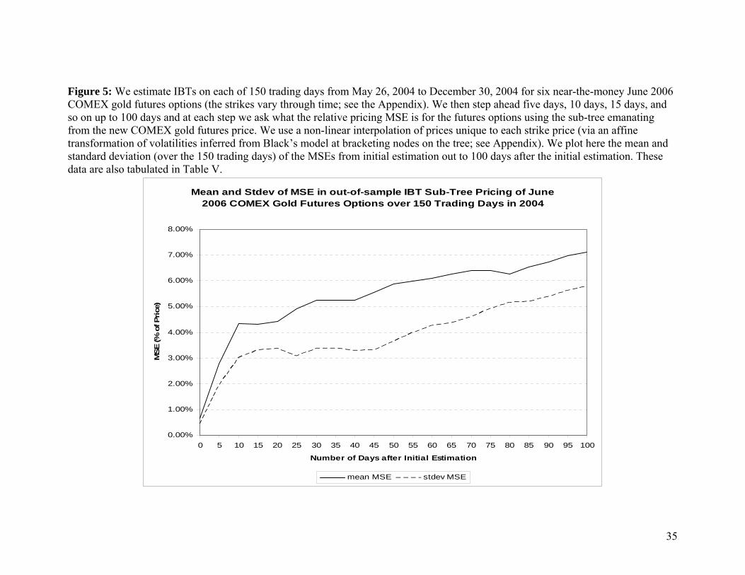
The initial average MSE pricing error of 0.65% (i.e., 65 basis points) increases quickly to
over 4% after 10 days, but then it increases relatively slowly after that reaching only
about 7% after 100 days (see Figure 5 and Table V for details).
(INSERT TABLE IV HERE)
The results are summarized as follows. First, the J-GIBT captures non-lognormal
properties of the underlying that are not reflected in either a CRR tree for the future spot
price, or in a CRR tree for the underlying based on the gold fix. Second, implementing
18
the J-GIBT using the Rubinstein and Smooth objective functions gives similar results
(and better behaved results than using the Jackwerth objective function). Third, the
implied trees can be calibrated to provide very accurate pricing of traded options and the
Jackwerth generalized weight function works well and is not far from linear. Fourth, real
option analysis that reflects a market consensus of the future (implied from traded
securities) can provide quite different real option valuation to the “standard” CRR
analysis. Finally, we present what we think is the first true out-of-sample test of an IBT
(in our appendix). This test shows how option pricing errors evolve on sub-trees
emanating from future levels of the underlying.
IX. Conclusion
This paper contains three main contributions to the literature. First, this is the first
application of an implied binomial tree (IBT) based on options traded on futures and not
traded on the spot. This allows for calibration of real option pricing models to non-
lognormal market consensus probability distributions of commodity prices. Second, one
of the criticisms of real option analysis is that capital budgeting decisions with long
planning horizons require long-horizon volatility estimates. In practice, these estimates
are difficult to obtain. Now, however, commodities IBTs using securities with very long
maturities can be estimated, and this means that long-horizon volatility estimates are now
freely available. Finally, we present the first out-of-sample illustration of how IBT
option pricing errors evolve when we look at sub-trees emanating from future levels of
the underlying.
19
APPENDIX (Out of Sample Sub-tree Pricing)
We were prompted by our referee to look at how well our IBT performs in a true out-of-
sample test. That is, we want to estimate the IBT model and then use it later to price the
same futures options on the sub-tree emanating from the node subsequently reached by
the futures price. We use June 2006 COMEX gold futures options traded during 2004.
These options were introduced mid year. The June 2006 option expirations in our sample
range from 729 days (on May 26, 2004, their first day’s trading) to 511 days (on Dec 30,
2004). There are exactly 150 trading days during 2004 when the June 2006 options trade.
We use essentially the same technique as that used in the main body of the paper with
three exceptions. First, rather than use Wall Street Journal T-bill yields, we use constant
maturity treasury yields drawn from DATASTREAM. These yields were for one-, two-,
and three-year maturities only, and we linearly interpolated to get yields for our
maturities. Second, unlike the short-dated options used in the main body of the paper, we
find that neither the Rubinstein nor Smooth objective functions perform well with the
long-dated options used in this appendix. We experience precisely the over-fitting
difficulties described by Jackwerth and Rubinstein (1996, p1623–1624). So, we use an
augmented objective function virtually identical to that described by Jackwerth and
Rubinstein (1996, p1624). We calibrate the penalty terms for this objective function using
the first five days of data; we keep these days in the sample because the estimations using
them seem no different from those on any other days. Third, with as many as 729 days to
expiration, we can no longer use 1-day steps in our binomial trees because they are too
computationally intensive to estimate. Instead, we choose to use five-day steps. In
practice, expirations are not in multiples of five days, so we round. For example, in the
20

case of 729 days to maturity, we use 146 steps, each of 4.993 calendar days. This means
that when we say below that we step out 100 days, say, from the initial estimation, we are
in fact stepping out 20 times 4.993 = 99.86 days; a minor approximation of no
importance.
For each of the 150 trading days, we estimate an IBT using six near-the money
gold futures options (the six strikes used vary through time as the futures price moves).
Given the estimated tree, we record the MSE of the relative pricing of the options. We
then step forward some multiple of five days (where the multiple is the number of steps
in the tree) and holding all parameters constant in the tree, we ask where the latest futures
price falls. Ideally, the futures price falls on an existing node of the tree, and we compare
the prices of the options on the tree at this node to the new market prices of the options.
In practice, there are three problems. First, the calendar day that occurs some multiple of
five calendar days later is not necessarily a trading day. Second, the new futures price is
almost never going to fall on an existing node of the tree, but will instead be bracketed by
two nodes, so some sort of interpolation of model prices is needed. Third, the new futures
price may be completely off the tree (i.e., not bracketed by two nodes of the tree). Let us
deal with each of these problems in turn.
First problem: if we step forward some multiple of five calendar days and find
that it is not a trading day, then our tree is providing prices for a day when no market
price can be observed for comparison. So, we step to the nearest trading day in the data
and record the futures and futures options prices on that day instead. We then ask how the
tree prices the options using these data at the calendar day node (which is then typically
only one calendar day away from the trading day whose data we use). This is a smaller
21

approximation than it may appear at first glance. For example, suppose our tree gives
options prices 40 days ahead, but that this day is a Saturday. We then use the futures and
futures options prices from the Friday. The options are so long dated and the structure of
the tree at day 40 is so similar to the structure at day 39 (one fifth of a step earlier), that as
long as the futures and futures options prices are from the same day, any approximation is
very minor and of no consequence for the MSE calculation. Note also that averaging our
MSEs over 150 different trees diversifies away any random discrepancies.
Second problem: suppose that the multiple-of-five-days ahead futures price falls
between two nodes of the tree (which it invariably does). How do we price the options at
this futures price on this day given that we have only discrete nodes available? We could
simply linearly interpolate between the options prices at the bracketing nodes, but we
know that options prices are not linear in the level of the underlying unless deep in- or
deep out-of-the-money. We need an interpolation technique that uses the existing tree and
takes non-linearity of pricing into account, but which also accommodates different-strike
options having different degrees of non-linearity in their pricing. Our solution is as
follows. Take the new futures price, and the first of our six options at the time step
we are focussing on in the tree. Now locate the nodes on the tree with futures prices
and that bracket the new futures price: . Now step
to the node and use the IBT model option price at that node and Black’s (1976)
futures options pricing model to back out an “implied volatility” for that strike at that
node:
NEWF
ABOVEF BELOWF BELOWNEWABOVE FFF >>
ABOVEF
ABOVEσ . Note that this is not a standard implied volatility because it is calculated
using IBT model prices, not market prices. That is, when ABOVEσ is plugged back into
Black’s model with , Black’s model returns the IBT model price at the ABOVEFF =
22
node ; no market prices of options are involved. We then step to the lower
bracketing node, , and we use the IBT model option price at that node and Black’s
futures options model to back out an implied volatility for that strike at that node:
ABOVEF
BELOWF
BELOWσ .
For clarity, let us again point out that when BELOWσ is plugged back into Black’s model
with , Black’s model returns the IBT model price at the node ; no
market prices of options are involved. We then take an affine combination of the two
implied volatilities:
BELOWFF = BELOWF
BELOWABOVE σαασ )1( −+ , where
)()( BELOWABOVEBELOWNEW FFFF −−≡α , and we plug this affine combination into Black’s
model to get an interpolated option value on the tree at . We do not revise the
Treasury yields used in Black’s model to match the new yields in the market because the
whole point of the exercise is to keep all parameters fixed and see how the tree performs
out of sample. We then repeat this (with different implied volatilities, of course) for the
next strike and so on. We then compare these interpolated sub-tree option prices to the
actual market option prices and calculate MSE of the relative pricing of the options. We
do this for each of the 150 trading days through the second half of 2004, and for each
multiple of five days out to 100 days from initial estimation.
NEWF
We have never seen this non-linear interpolation technique used before, and we
like it for several reasons. This technique uses only data from the initial estimation (apart
from , of course). It also guarantees that if falls precisely on a node, then the
affine combination implied volatility when plugged into Black’s model returns exactly
the IBT model option value at that node. It also captures the non-linearity of the
NEWF NEWF
23

relationship between option price and underlying, and it allows for this non-linearity to be
different for all strikes.
Third problem: we find that in seven out of the 150 trees, the new futures price is
not bracketed by two nodes on the tree but only at the first five-day-ahead step. In all
other trees, and at all other steps, the futures price is within the tree and bracketed by two
nodes. We simply exclude these seven observations from the analysis (note the different
sample size at day five in Table V).
We record the MSE at the initial estimation and at every five-day step out to 100
days ahead. Table V reports the sample size, mean, and standard deviation of these MSEs
over the 150 estimated trees. Figure 5 plots the mean and standard deviation of these
MSEs over the 150 estimated trees. Note that the 150 observations of MSE at any fixed
multiple of five days are not independent of each other. The trees overlap so much
through time that the observations of MSE at a fixed distance from the initial estimation
are positively auto-correlated through time. The further ahead we look in the trees (e.g.,
50 days ahead versus 40 days ahead), the greater the relative overlap of the trees and the
greater the auto-correlation in the MSEs at that many steps ahead through the 150-day
sample. For example, the auto-correlation in the MSEs through time increases from
31.1% at the initial estimation, to 40.8% at the five-day step, to 56.8% at the 10-day step,
and so on up to 92.8% at the 100-day step; it is almost monotonic. The means and
standard deviations in Table V and Figure 5 are not biased. The dependence means,
however, that you cannot divide the standard deviation of the MSEs by the square root of
the sample size to get a standard error on the mean MSE.
24

Looking at Table V and Figure 5, we see that the MSE rises quite rapidly from the
initial estimation MSE of 0.65% out to 2.81% after five days, then 4.34% after 10 days.
The MSE continues to rise, not quite monotonically, and not as rapidly, out to 100 days
where it is about 7.12%. The fall off in the rate of climb of the MSE may be partly
because the number of nodes is increasing as we move further from the initial estimation.
For example, at the five-day-ahead step, there are only two nodes on the tree (because we
are using steps of five days for these long-dated options).
The rise in MSE is, of course, in line with our intuition that pricing on sub-trees
should be less accurate as time passes. The rise in MSE is in fact less pronounced than we
were expecting. We have not seen this sort of out-of-sample sub-tree pricing performed
anywhere else using IBTs. Analysts can now see for the first time, in our Figure 5, how
pricing errors evolve through time on an increasingly stale IBT. This does not mean that
the initial pricing is bad, just that the markets changed in ways that were not anticipated
(changes in volatility most likely).
25
Bibliography
Black, Fischer. “The Pricing of Commodity Contracts.” The Journal of Financial Economics, 3 (1/2) (January/March 1976), 167–179. Black, Fisher and Myron Scholes. “The Pricing of Options and Corporate Liabilities.” Journal of Political Economy, 81 (May/June 1973), 637–659. Carmona, Rene and Michael Ludkovski. “Spot Convenience Yield Models for the Energy Markets.” Working Paper, Princeton, Nov 06, 2003. http://www.orfe.princeton.edu/~rcarmona/fepreprints.html Chriss, Neil A., Black-Scholes and Beyond: Option Pricing Models, MCGraw-Hill: New York, NY (1997). Cox, John, Stephen Ross, and Mark Rubinstein. “Option Pricing: A Simplified Approach.” Journal of Financial Economics, 7(3) (1979), 229– 263. Derman, Emanuel and Iraj Kani. “The Volatility Smile and its Implied Tree.” Goldman Sachs Quantitative Strategies Research Notes, Goldman, Sachs, (January 1994). Gibson, Rajna, and Eduardo S. Schwartz. “Stochastic Convenience Yield and the Pricing of Oil Contingent Claims.” Journal of Finance, 45(3) (July 1990), 959–976. Hilliard, Jimmy, Jorge Reis. “Valuation of Commodity Futures and Options under Stochastic Convenience Yields, Interest Rates, and Jump Diffusions in the Spot.” Journal of Financial and Quantitative Analysis, 33(1) (March 1998), 61–86. Hull, John C. Options, Futures, and Other Derivatives. Fourth Edition, Prentice-Hall: Upper Saddle River, NJ (2000). Jackwerth, Jens Carsten and Mark Rubinstein. “Recovering Probability Distributions from Option Prices.” Journal of Finance, 51(5) (1996), 1611–1631. Jackwerth, Jens Carsten. “Generalized Binomial Trees,” Journal of Derivatives, 5(2) (1997), 7–17. Jackwerth, Jens Carsten. “Option-Implied Risk-Neutral Distributions and Implied Binomial Trees: A Literature Review.” Journal of Derivatives, 7(2) (1999), 66–81. Miltersen, Kristian R., “Commodity Price Modelling that Matches Current Observables: A New Approach,” Working Paper, January 30, 2003 Miltersen and Schwartz. “Pricing of Options on commodity futures with Stochastic Term Structures of convenience Yields and Interest rates.” Journal of Financial and Quantitative Analysis, 33(1) (March 1998) 33–59.
26

27
Rubinstein, Mark. “Implied Binomial Trees.” Journal of Finance, 49(3) (1994), 771–818. Trigeorgis, Lenos. Real Options: Managerial Flexibility and Strategy in Resource Allocation, MIT Press. Cambridge, MA (1996).
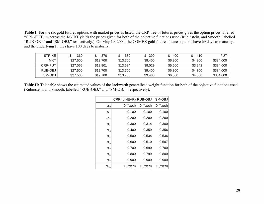
Table I: For the six gold futures options with market prices as listed, the CRR tree of futures prices gives the option prices labelled “CRR-FUT,” whereas the J-GIBT yields the prices given for both of the objective functions used (Rubinstein, and Smooth, labelled “RUB-OBJ,” and “SM-OBJ,” respectively.). On May 19, 2004, the COMEX gold futures futures options have 69 days to maturity, and the underlying futures have 100 days to maturity.
STRIKE $ 360 $ 370 $ 380 $ 390 $ 400 $ 410 FUTMKT $27.500 $19.700 $13.700 $9.400 $6.300 $4.300 $384.000
CRR-FUT $27.065 $19.801 $13.684 $9.029 $5.600 $3.242 $384.000 RUB-OBJ $27.500 $19.700 $13.700 $9.400 $6.300 $4.300 $384.000
SM-OBJ $27.500 $19.700 $13.700 $9.400 $6.300 $4.300 $384.000 Table II: This table shows the estimated values of the Jackwerth generalized weight function for both of the objective functions used (Rubinstein, and Smooth, labelled “RUB-OBJ,” and “SM-OBJ,” respectively).
CRR (LINEAR) RUB-OBJ SM-OBJ
0α 0 (fixed) 0 (fixed) 0 (fixed)
1α 0.100 0.100 0.100
2α 0.200 0.200 0.200
3α 0.300 0.314 0.300
4α 0.400 0.359 0.356
5α 0.500 0.534 0.536
6α 0.600 0.510 0.507
7α 0.700 0.690 0.700
8α 0.800 0.799 0.800
9α 0.900 0.900 0.900
10α 1 (fixed) 1 (fixed) 1 (fixed)
28
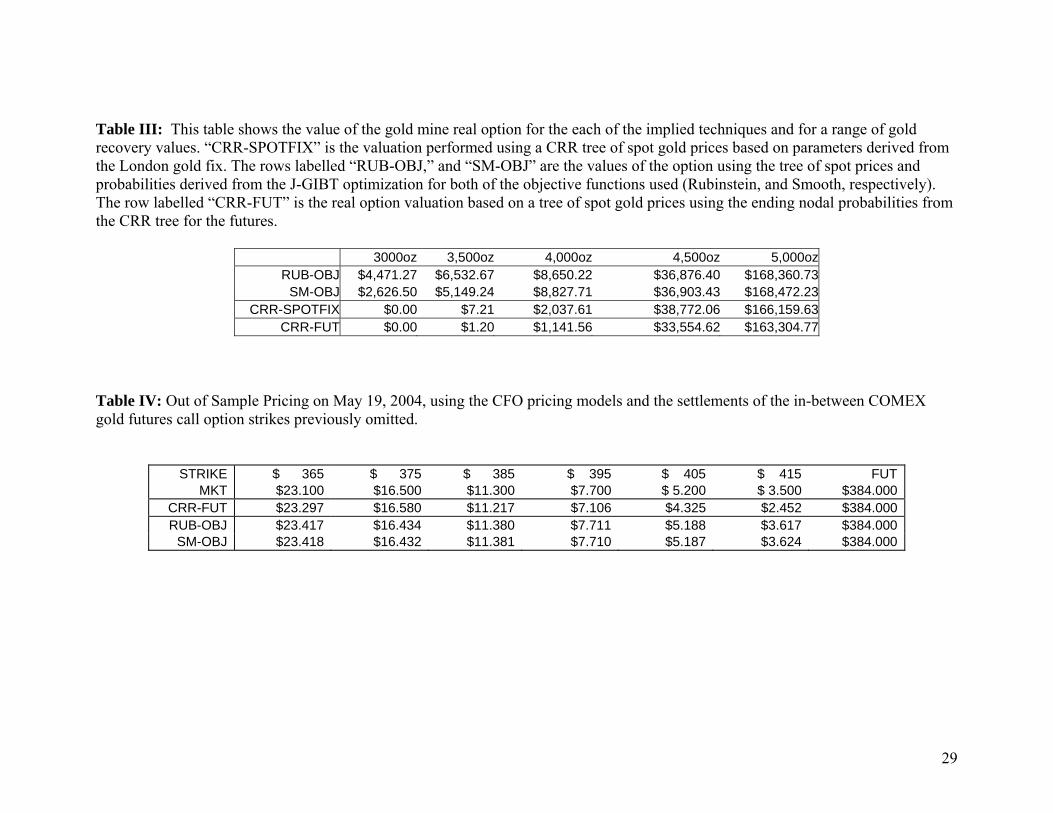
Table III: This table shows the value of the gold mine real option for the each of the implied techniques and for a range of gold recovery values. “CRR-SPOTFIX” is the valuation performed using a CRR tree of spot gold prices based on parameters derived from the London gold fix. The rows labelled “RUB-OBJ,” and “SM-OBJ” are the values of the option using the tree of spot prices and probabilities derived from the J-GIBT optimization for both of the objective functions used (Rubinstein, and Smooth, respectively). The row labelled “CRR-FUT” is the real option valuation based on a tree of spot gold prices using the ending nodal probabilities from the CRR tree for the futures.
3000oz 3,500oz 4,000oz 4,500oz 5,000ozRUB-OBJ $4,471.27 $6,532.67 $8,650.22 $36,876.40 $168,360.73
SM-OBJ $2,626.50 $5,149.24 $8,827.71 $36,903.43 $168,472.23CRR-SPOTFIX $0.00 $7.21 $2,037.61 $38,772.06 $166,159.63
CRR-FUT $0.00 $1.20 $1,141.56 $33,554.62 $163,304.77 Table IV: Out of Sample Pricing on May 19, 2004, using the CFO pricing models and the settlements of the in-between COMEX gold futures call option strikes previously omitted.
STRIKE $ 365 $ 375 $ 385 $ 395 $ 405 $ 415 FUTMKT $23.100 $16.500 $11.300 $7.700 $ 5.200 $ 3.500 $384.000
CRR-FUT $23.297 $16.580 $11.217 $7.106 $4.325 $2.452 $384.000 RUB-OBJ $23.417 $16.434 $11.380 $7.711 $5.188 $3.617 $384.000
SM-OBJ $23.418 $16.432 $11.381 $7.710 $5.187 $3.624 $384.000
29
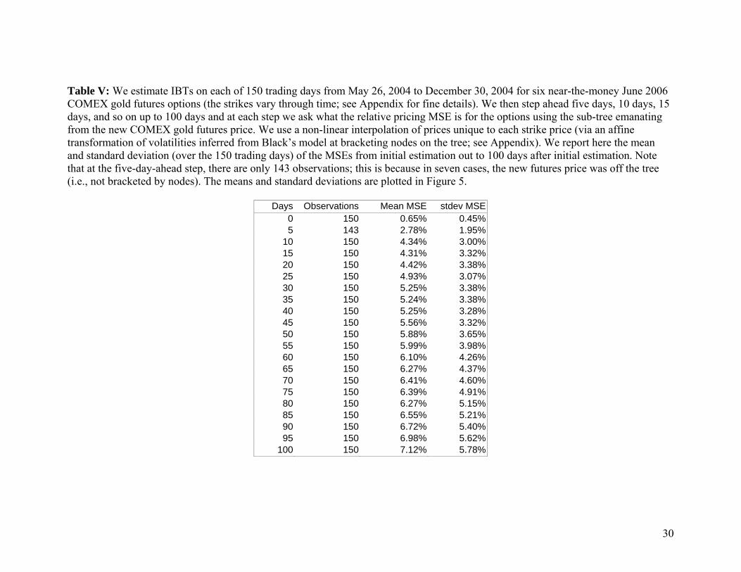
Table V: We estimate IBTs on each of 150 trading days from May 26, 2004 to December 30, 2004 for six near-the-money June 2006 COMEX gold futures options (the strikes vary through time; see Appendix for fine details). We then step ahead five days, 10 days, 15 days, and so on up to 100 days and at each step we ask what the relative pricing MSE is for the options using the sub-tree emanating from the new COMEX gold futures price. We use a non-linear interpolation of prices unique to each strike price (via an affine transformation of volatilities inferred from Black’s model at bracketing nodes on the tree; see Appendix). We report here the mean and standard deviation (over the 150 trading days) of the MSEs from initial estimation out to 100 days after initial estimation. Note that at the five-day-ahead step, there are only 143 observations; this is because in seven cases, the new futures price was off the tree (i.e., not bracketed by nodes). The means and standard deviations are plotted in Figure 5.
Days Observations Mean MSE stdev MSE0 150 0.65% 0.45%5 143 2.78% 1.95%
10 150 4.34% 3.00%15 150 4.31% 3.32%20 150 4.42% 3.38%25 150 4.93% 3.07%30 150 5.25% 3.38%35 150 5.24% 3.38%40 150 5.25% 3.28%45 150 5.56% 3.32%50 150 5.88% 3.65%55 150 5.99% 3.98%60 150 6.10% 4.26%65 150 6.27% 4.37%70 150 6.41% 4.60%75 150 6.39% 4.91%80 150 6.27% 5.15%85 150 6.55% 5.21%90 150 6.72% 5.40%95 150 6.98% 5.62%
100 150 7.12% 5.78%
30
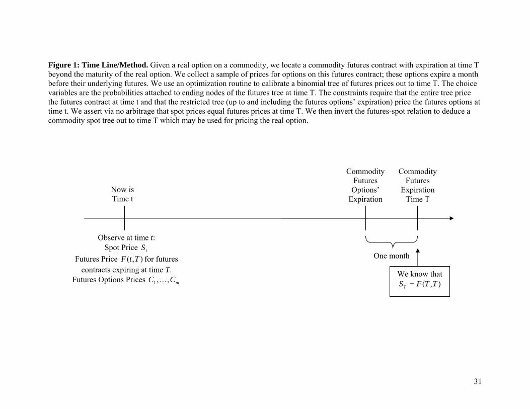
Figure 1: Time Line/Method. Given a real option on a commodity, we locate a commodity futures contract with expiration at time T beyond the maturity of the real option. We collect a sample of prices for options on this futures contract; these options expire a month before their underlying futures. We use an optimization routine to calibrate a binomial tree of futures prices out to time T. The choice variables are the probabilities attached to ending nodes of the futures tree at time T. The constraints require that the entire tree price the futures contract at time t and that the restricted tree (up to and including the futures options’ expiration) price the futures options at time t. We assert via no arbitrage that spot prices equal futures prices at time T. We then invert the futures-spot relation to deduce a commodity spot tree out to time T which may be used for pricing the real option.
Now is Time t
Commodity Futures Options’
Commodity Futures
Expiration Expiration Time T
One month
We know that ),( TTFST =
Observe at time t: SSpot Price
,( TtFt
Futures Price for futures contracts expiring at time T.
CC ,,K
)
Futures Options Prices m1
31
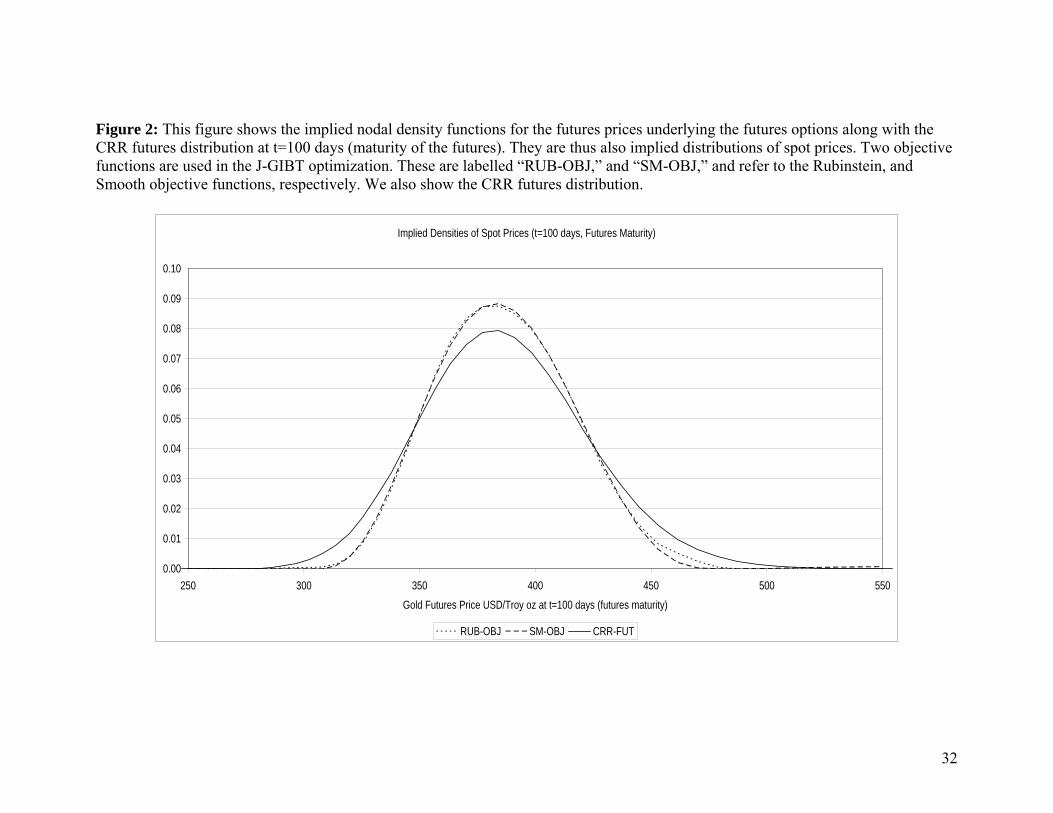
Figure 2: This figure shows the implied nodal density functions for the futures prices underlying the futures options along with the CRR futures distribution at t=100 days (maturity of the futures). They are thus also implied distributions of spot prices. Two objective functions are used in the J-GIBT optimization. These are labelled “RUB-OBJ,” and “SM-OBJ,” and refer to the Rubinstein, and Smooth objective functions, respectively. We also show the CRR futures distribution.
Implied Densities of Spot Prices (t=100 days, Futures Maturity)
0.00
0.01
0.02
0.03
0.04
0.05
0.06
0.07
0.08
0.09
0.10
250 300 350 400 450 500 550
Gold Futures Price USD/Troy oz at t=100 days (futures maturity)
RUB-OBJ SM-OBJ CRR-FUT
32
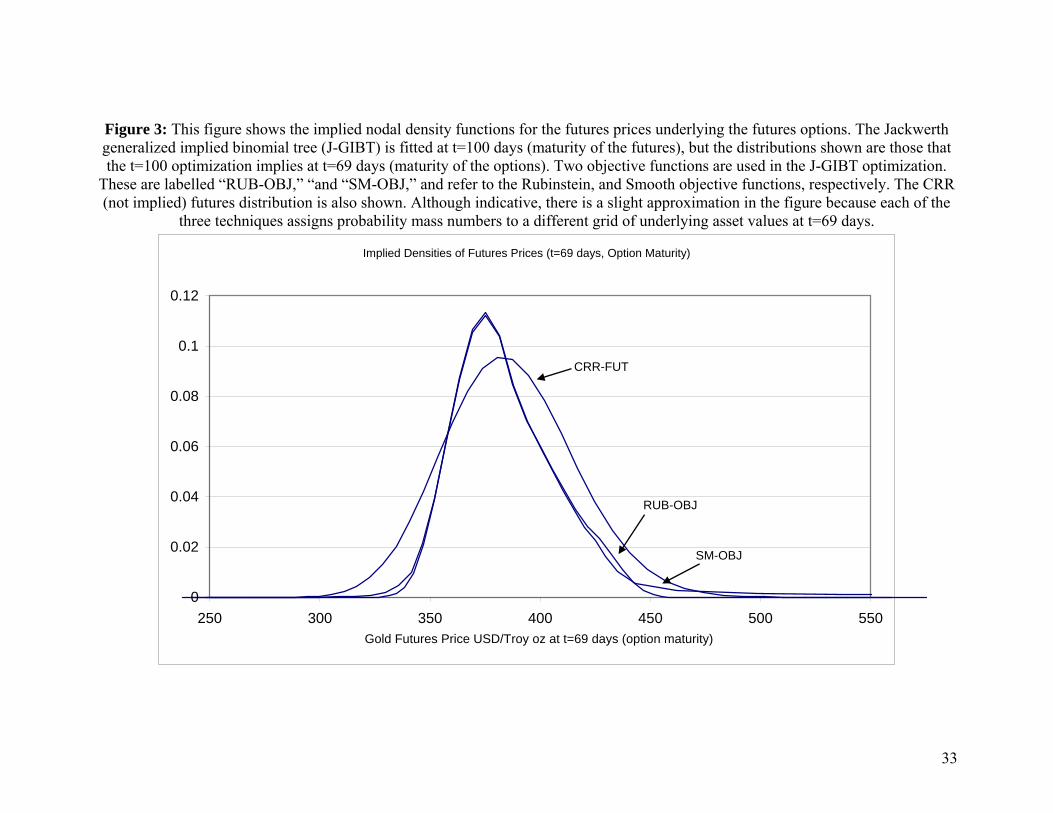
Figure 3: This figure shows the implied nodal density functions for the futures prices underlying the futures options. The Jackwerth generalized implied binomial tree (J-GIBT) is fitted at t=100 days (maturity of the futures), but the distributions shown are those that the t=100 optimization implies at t=69 days (maturity of the options). Two objective functions are used in the J-GIBT optimization.
These are labelled “RUB-OBJ,” “and “SM-OBJ,” and refer to the Rubinstein, and Smooth objective functions, respectively. The CRR (not implied) futures distribution is also shown. Although indicative, there is a slight approximation in the figure because each of the
three techniques assigns probability mass numbers to a different grid of underlying asset values at t=69 days.
Implied Densities of Futures Prices (t=69 days, Option Maturity)
0
0.02
0.04
0.06
0.08
0.1
0.12
250 300 350 400 450 500 550Gold Futures Price USD/Troy oz at t=69 days (option maturity)
CRR-FUT
RUB-OBJ
SM-OBJ
33
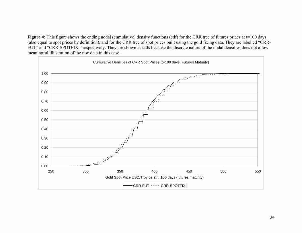
Figure 4: This figure shows the ending nodal (cumulative) density functions (cdf) for the CRR tree of futures prices at t=100 days (also equal to spot prices by definition), and for the CRR tree of spot prices built using the gold fixing data. They are labelled “CRR-FUT” and “CRR-SPOTFIX,” respectively. They are shown as cdfs because the discrete nature of the nodal densities does not allow meaningful illustration of the raw data in this case.
Cumulative Densities of CRR Spot Prices (t=100 days, Futures Maturity)
0.00
0.10
0.20
0.30
0.40
0.50
0.60
0.70
0.80
0.90
1.00
250 300 350 400 450 500 550
Gold Spot Price USD/Troy oz at t=100 days (futures maturity)
CRR-FUT CRR-SPOTFIX
34
35
Figure 5: We estimate IBTs on each of 150 trading days from May 26, 2004 to December 30, 2004 for six near-the-money June 2006 COMEX gold futures options (the strikes vary through time; see the Appendix). We then step ahead five days, 10 days, 15 days, and so on up to 100 days and at each step we ask what the relative pricing MSE is for the futures options using the sub-tree emanating from the new COMEX gold futures price. We use a non-linear interpolation of prices unique to each strike price (via an affine transformation of volatilities inferred from Black’s model at bracketing nodes on the tree; see Appendix). We plot here the mean and standard deviation (over the 150 trading days) of the MSEs from initial estimation out to 100 days after the initial estimation. These data are also tabulated in Table V.
Mean and Stdev of MSE in out-of-sample IBT Sub-Tree Pricing of June 2006 COMEX Gold Futures Options over 150 Trading Days in 2004
0.00%
1.00%
2.00%
3.00%
4.00%
5.00%
6.00%
7.00%
8.00%
0 5 10 15 20 25 30 35 40 45 50 55 60 65 70 75 80 85 90 95 100
Number of Days after Initial Estimation
MSE
(% o
f Pri
ce)
mean MSE stdev MSE

Footnotes 1 To be precise, the lognormal assumption is true only in the limit as step size goes to
zero in a traditional binomial tree. For non-infinitesimal time steps, the distribution of
asset price is only approximately lognormal in the traditional binomial tree.
2 One other benefit of IBTs that is not often pointed out is that, by construction, the local
volatility of the underlying is allowed to vary through the binomial tree (Rubinstein,
1994, p795). This is another relaxation of the traditional binomial tree’s assumptions.
3 Note that if a contract is so long dated that it is beyond the limits of active trade, then its
settlement price is determined at day’s end by a committee on the floor based on the final
set of trade prices (personal communication with COMEX staff by telephone May 2005).
These prices are not stale (they are revised every day), but they may suffer from liquidity
issues. The implied distributions for the long-dated options used in the Appendix suggest
that no simple pricing model is being used, but that these prices genuinely represent
market consensus views.
4 Readers interested in continuous time implementations that model stochastic
convenience yields with mean reversion should consult Miltersen and Schwartz (1998),
Carmona and Ludkovski (2003), and Miltersen (2003).
5 For example, the NYMEX trades futures options on light sweet crude oil, natural gas,
heating oil, gasoline, Brent crude oil, propane, coal, electricity, gold, silver, copper,
aluminum, platinum, and palladium; the CBOT trades futures on corn, soybeans, wheat,
oats, rice, gold and silver; and the CME trades futures options on beef, dairy, hogs and
lumber. The LIFFE trades futures options on cocoa, coffee, wheat, and white sugar.
36

6 Another alternative is to think entirely in terms of futures prices. An implied binomial
tree could be created for futures prices using the J-GIBT method and the American-style
futures options. The gain or loss on the futures contract can be estimated if the gold is
physically delivered. This restricts valuation to real options where you will in fact make
or take delivery of the underlying using futures.
7 We linearly interpolate between the continuously-compounded yields on the T-bills of
maturities bracketing the maturity of the futures. These continuous yields are calculated
using the midpoints of the WSJ quoted bid-ask spreads as per Cox and Rubinstein (1985,
p255). These yields are in fact not used to construct the futures tree, but to deduce
theδ and to value the futures options.
8 For ending nodes numbered from 0 (lowest futures price) up to 100 (highest futures
price) these probabilities are du
dp
−
−=
1'[ ]{ } jnpjpjnjnjP −−−= )'1(')!(!/!' where and
teu ∆= σ ted ∆−= σand are the growth factors. Note that the risk-neutral drift of the
futures is zero.
9 We do not use the original Jackwerth (1997) objective function (using squared
deviations of model option prices from market option prices). It lacks any form of
regularity condition regarding shape of the distribution and it consequently produces
spiky non-credible implied distributions.
10 Think about valuing the futures contract, as opposed to finding the futures price: the
value must be zero. If there is no interest on the margin account, then the value (i.e., 0) is
just ∑P_j [F(T,T)_j-F(t,T)]. Thus, F(t,T)=∑P_jF(T,T),j with no discounting and the drift
is zero. Alternatively, let * denote RN expectation, then E*[F(T,T)|F(t,T),S(t)] must equal
37

E*[S(T)|F(t,T),S(t)] by no arbitrage at time T. But the latter is just F(t,T). Thus F(t,T)=
E*[F(T,T)|F(t,T),S(t)] and there is no drift.
11 It is here that we should technically have used the Treasuries for the maturity of the
options as opposed to the futures.
12 London AM Gold Fix data are taken from www.kitco.com from Feb 20, 2004 to May
19, 2004.
13 The daily standard deviation is 0.0122665400, and multiplied by square root of 252
gives an annualised number of σ =0.194725286. The 100-day futures price and the T-bill
yield of r=1.0509% are used to deduce an annualised convenience yield of -0.139%=δ .
The CRR tree for spot gold is then built using ( )[ ]
du
dtrep
−
−∆−=
δ and u and d as per usual.
14 Calibrating the CRR futures tree with a volatility that forces the tree to price the at-the-
money option precisely does not change any of the other qualitative properties of the
results.
15 We used several “clamping” techniques to flatten out the small probability mass sitting
in the extreme tails of the implied distributions. In all cases, clamping down on a tail of
the distribution produces an extra modal hump close to the central mode (not shown here
but very similar to Jackwerth and Rubinstein, 1996, Figure 4, p1627). The qualitative
behavior of the implied versus CRR techniques in Table III was completely robust to the
use of clamping methods. This robustness convinces us that the presence of a small
probability mass in the tails of the implied distributions is a genuine reflection of a
market consensus view on large price moves, and not any form of statistical artifact.
38