State of New JerseyNew Jersey Department of Environmental ProtectionJon S. Corzine, GovernorLisa P. Jackson, Commissioner

April 2007

Valuing New Jersey’s Natural Capital:An Assessment of the Economic Value of the State’s Natural Resources

Valuing New Jersey’s Natural Capital:An Assessment of the Economic Value of the State’s Natural Resources

PART III:

NATURAL GOODS

State of New JerseyNew Jersey Department of Environmental Protection

Jon S. Corzine, GovernorLisa P. Jackson, Commissioner

April 2007

2

Table of Contents

ACKNOWLEDGMENTS.................................................................................................................................. 3

EXECUTIVE SUMMARY................................................................................................................................ 4

I. OVERVIEW AND SCOPE............................................................................................................................ 8

II. ECONOMIC VALUE OF NATURAL GOODS ........................................................................................... 11

III. WATER RESOURCES............................................................................................................................ 16Water demand ..................................................................................................................................... 17Water supply ....................................................................................................................................... 18Conclusions on water flow.................................................................................................................. 22Commercial value of water ................................................................................................................. 23Economic value of water..................................................................................................................... 25

IV. MINERAL RESOURCES........................................................................................................................ 30

V. AGRICULTURAL PRODUCTS ................................................................................................................. 36 Market value of farm products............................................................................................................ 37 Market value of farmland.................................................................................................................... 38

VI. NON-FARM ANIMALS.......................................................................................................................... 42

VII. NON-FARM PLANTS........................................................................................................................... 45

VIII. FISH AND SHELLFISH ....................................................................................................................... 47 Commercial fishing ............................................................................................................................. 47

Recreational fishing ............................................................................................................................ 54

IX. FUELWOOD AND SAWTIMBER ............................................................................................................ 58Fuelwood............................................................................................................................................. 58Sawtimber............................................................................................................................................ 61

X. SUMMARY AND CONCLUSIONS ............................................................................................................ 65

APPENDIX A: ESTIMATION OF TOTAL ECONOMIC VALUE.................................................................... 72

APPENDIX B: ELASTICITY IN LINEAR DEMAND FUNCTIONS................................................................. 82

APPENDIX C: ALTERNATE FARMLAND VALUATIONS............................................................................ 83

APPENDIX D: VALUATION OF STANDING SAWTIMBER.......................................................................... 86

EXHIBITS .................................................................................................................................................... 88

REFERENCES .............................................................................................................................................. 92

3

AcknowledgmentsA number of persons in various government agencies and universities provided invaluableassistance in the preparation of this report, of whom the following deserve particular mention;unless otherwise indicated, the person named is on the staff of the New Jersey Department ofEnvironmental Protection (NJDEP). Any errors in the interpretation of the information thesepersons provided are the responsibility of the author.

General assistance Mary Kearns-Kaplan and Jorge Reyes, NJDEP

Water supply data Jeff Hoffman and Steve Domber, NJDEP

Retail water rates Dante Mugrace, Charlene Good, and Renee GoodNew Jersey Board of Public Utilities

Mineral resources Dr. Lloyd Mullikin, NJDEP

Agricultural data Roger Strickland and Larry Traub, U.S. Department of Agriculture

Timber resources Richard Widmann and Douglas Griffith, U.S. Forest Service

Timber demand Dr. Adam Daigneault, U.S. Environmental Protection Agency

Valuation methods Dr. Peter Parks, Rutgers UniversityDr. Hilary Sigman, Rutgers UniversityDr. Robert Young, Colorado State UniversityDr. Robert Costanza, University of VermontDr. Steven Farber, University of Pittsburgh

This study was prepared by William Mates, Research Scientist, NJDEP. Martin Rosen ofNJDEP reviewed the report in its each of its successive drafts and provided valuable comments.Jeanne Herb of NJDEP initiated the study and provided general direction and support.

4

Executive Summary

I. Overview and Scope

Part III of this three-part report on New Jersey’s natural capital deals with the natural goodsprovided by New Jersey’s natural assets, i.e., its living and non-living environment. The conceptsof natural capital and natural assets emphasize the fact that the natural environment, like anyother capital asset, provides a stream of economic benefits over an extended period of time;given maintenance of that capital and sustainable harvest levels, those benefits can in principlebe generated in perpetuity. The natural goods dealt with are divided into seven categories foranalytic purposes: water, minerals, farm products, non-farm animals, non-farm plants, fish, andwood. This report is careful not to double-count ecosystem services covered in Part II.

II. Determination of Economic Value

Total Economic Value (or Total Willingness to Pay) has two main components: Market Valueand Consumer Surplus. Consumer Surplus is the amount that consumers would be willing to payfor a natural good but do not actually have to pay. Market Value can be obtained from officialand quasi-official data for all of the natural goods discussed in this report; Consumer Surplus,however, must be estimated. Economists have developed various ways of generating suchestimates, but many of those methods require data that is not readily available or involvemathematical techniques that result in implausibly high estimates of Consumer Surplus. Thisreport uses a more conservative approach based on the assumption of a linear demand functionand a point estimate of elasticity of demand; this approach allows Consumer Surplus to beestimated based solely on Market Value and elasticity.

III. Water Resources

Based on information in the 1996 Statewide Water Supply Plan, New Jersey’s naturalenvironment provides between 494 and 579 billion gallons of raw (unprocessed) water annually.1That resource has an estimated in situ market value of $0.394 per 1,000 gallons. In order tomeasure only the value of the water itself, that figure excludes the costs of treating the water anddelivering it on demand to end users. Based on the methodology described in Section II andAppendix A the Total Economic Value of that water in 2004 dollars is estimated to fall between$262 and $696 million/year (central estimate = $385 million/year), including the estimatedConsumer Surplus. The present value of that benefit stream is between $9 and $23 billion(central estimate = $13 billion), based on conventional discounting at 3%/year in perpetuity.These values are subject to change based on changes in land use, climate, and other factors.

IV. Mineral Resources

According to 2004 data from the United States and New Jersey Geological Surveys, NewJersey’s mines and quarries provide an average of $321 million in Market Value annually inconstruction and industrial sand and gravel and crushed stone. (That figure excludes a significantamount of sand dredged offshore by the U.S. Army Corps of Engineers for use in beach 1 To avoid double-counting, these figures are net of water used for agriculture (including irrigation).

5

replenishment.) In order to measure only the value of the minerals themselves, the $320.9Mfigure excludes the costs of delivering them to end users. The Total Economic Value of thatannual output in 2004 dollars is estimated at between $481 million/year and $1.1 billion/year(central estimate = $587 million/year), including the related Consumer Surplus. The presentvalue of that benefit stream is between $16 and $37 billion (central estimate = $20 billion. Thesevalues are subject to change based on changes in extraction rates, which in turn depend on thedemand for these materials.

V. Agricultural Products

Based on information from the U.S. Department of Agriculture, New Jersey’s farms providedplant and animal products with a total Market Value of $787 million in 2004 dollars or $108million net of farm production costs. The Total Economic Value of that annual output in 2004dollars is estimated to be about $6.5 billion/year ($885 million net of production costs), includingthe related Consumer Surplus. The present value of that benefit flow is estimated at about $216billion ($30 billion net of production costs). These values are highly dependent on land use,climate, and other factors and may decline as farmland is converted to other uses.

VI. Non-Farm Animals

Game animals and birds and fur-bearing animals harvested in New Jersey have an annual marketvalue of about $3 million, based on volume data from NJDEP’s Division of Fish and Wildlifeand prices for related meat products in the Northeastern U.S. (The retail prices provided by theU.S. Bureau of Labor Statistics were adjusted to approximate wholesale prices.) The TotalEconomic Value of that annual output in 2004 dollars is estimated to be about $21 million/year,including the related Consumer Surplus, and the present value of that flow of benefits isestimated at about $703 million. The maintenance of these values depends on the stability of landuse patterns, hunting policies and practices, and other factors.

VII. Fish and Shellfish

New Jersey’s commercial fishing vessels harvest finfish and shellfish with a total averageMarket Value of about $123 million/year, according to data from the National Marine FisheriesService. Of that amount, shellfish represent about 62% by weight and 85% by value. This harvesthas an estimated Total Economic Value in 2004 dollars of about $750 million/year, including theestimated Consumer Surplus. The present value of that benefit stream is estimated at about $25billion. These values are subject to change based on changes in fish stocks, consumer demand,and other factors.

New Jersey’s recreational anglers harvest saltwater and freshwater fish with a total averageMarket Value estimated at about $34 million/year, according to data from various sources. Thisharvest has an estimated Total Economic Value in 2004 dollars of about $207 million/year,including the related Consumer Surplus; the present value of that benefit stream is estimated atabout $7 billion. As with commercial fisheries, these values are subject to change based onchanges in fish stocks, fishing regulations, and other factors.

6

VIII. Non-Farm Plants

New Jersey’s landscapes provide an unknown amount of useful non-farm plants, includingflowers, medicinal plants, and others. The data on these products are meager, and it is notcurrently feasible to estimate their economic value. Methods are being developed to estimatesuch values (where volume data are available), but those methods are still in the developmentalstage.

IX. Timber and Fuelwood

In 2003, New Jersey used about 1.6 million cords of wood and wood wastes as an energy source,primarily for electric power generation and residential heating. The share of that fuelwoodoriginating in New Jersey cannot be determined, and this analysis assumes that 100% of it comesfrom in-state sources. Based on a value of $23.48/cord in 2004 dollars, 2003 consumption had aMarket Value of about $39 million/year and a Total Economic Value of about $95 million/year(including Consumer Surplus), for a present value of about $3 billion.

Between 1987 and 1999, New Jersey’s marketable timber resources increased by an average of204 million board-feet/year, of which hardwoods (i.e., deciduous trees) represented about 89%.Based on wholesale prices for the various tree species, that annual growth had a Market Value of$49 million/year in 2004 dollars. Including Consumer Surplus, this represents a Total EconomicValue of between $96 and $293 million/year (central estimate = $147 million/year) and a presentvalue of between $3 and $10 billion (central estimate = $5 billion). Whether the growth rate ofthe 1987-1999 period continued after 1999 is not known. The maintenance of that growth rateand therefore the above value estimates depends on a variety of factors, including land usechange, climate change, harvest policies, species mix, tree disease patterns, and others.

X. Summary and Limitations

The values presented above total $1.2 billion/year in terms of Market Value (range $820 millionto $1.6 billion/year) and $5.9 billion/year in Total Economic Value (range $2.8-9.7 billion/year);the difference between Market Value and Total Value represents Consumer Surplus. Based onthese flows of value, New Jersey’s natural capital has an estimated worth of $196 billion inpresent value terms (range $93-322 billion). Farm products and fish command the largest shares,followed by minerals and raw water; wood (including both sawtimber and fuelwood) and non-farm animals have the lowest shares, while the value of non-farm plants was not estimated.

The value provided varies by ecosystem, depending on the types of natural goods provided, thetotal acreage of the ecosystem, and the average value per acre. The value provided varies byecosystem, depending on the types of natural goods provided, the total acreage of the ecosystem,and the average value per acre. Farmland and marine ecosystems generate the highest values interms of total value, followed by barren land (which includes mines and quarries), forests, andfreshwater wetlands. In terms of value per acre, non-ecosystem land (mines and quarries) ranksfirst, followed by farmland, marine ecosystems, and open fresh waters.

7

The results of this study should be treated as first estimates and not as final definitive valuations.For various reasons, the results do not include secondary economic benefits supported by directexpenditures on natural goods, including such secondary benefits as the economic activitysupported by spending by employees in agriculture, retail food distribution, commercial fishing,mining, timber and timber-using industries, etc. These omissions lead to an understatement oftotal economic value. On the other hand, the results of the study do include producer costs,resulting in an overstatement of net economic value.

Future research should focus on the following:

• All ecosystems: more current land use/land cover data.• All ecosystems: relationships between production of services and goods.• Water: more current data on supplies and leakage rates.• Minerals: tonnage and market value of sand dredged offshore.• Farm products: more recent data on the amount of farmland by type.• Fish: prices for recreational freshwater species; role of wetlands.• Non-farm plants: data and methods for preparing rough valuations.• Fuelwood: share of wood harvested in-state; estimated sustainable yield.• Timber: more current annual growth data; estimates of sustainable yield.• All natural goods: further research on relative per-acre ecosystem productivity.• All natural goods: further research on elasticity of demand.

A valuation study such as this one can never be regarded as a closed book, any more than avaluation analysis in business or any other sphere: as conditions change, so do values, and theprocess of change is continuous. Nonetheless, it is clear that New Jersey’s natural capital, bothliving and non-living, makes a substantial contribution every year to New Jersey’s economy andquality of life by providing natural goods worth several billion dollars both annually and inpresent value terms.

8

Section I: Overview and Scope

Part II of this three-part report described in detail the valuation methods applied to theservices provided by New Jersey’s ecosystems and presented the results of those valuations; PartIII does the same for ecosystem and abiotic goods (together termed “natural goods”). As Table 1(next page) shows, New Jersey’s ecosystems and the state’s non-living natural capital provide avariety of economically important natural goods; for purposes of analysis and presentation, thesehave been grouped into the seven categories shown. While each of these categories include manyspecific goods, the categories themselves will frequently be referred to as “natural goods”.

As Table 1 indicates, all of the natural goods considered in this report are provided by morethan one ecosystem, and in some cases, it is difficult to allocate the total value of natural goodsamong the relevant ecosystems, as these examples show:

• “Groundwater recharge areas” are not identifiable as such from aerial photographs;rather, they exhibit one of the standard land cover types, e.g., forest or meadow.However, it cannot be assumed a priori that all forested lands function as recharge areas.In addition, surface waters and underground aquifers are usually hydrologicallyconnected, so that some part of “groundwater” recharge is attributable to surface watersand vice versa.

• While forests produce more fuelwood than forested wetlands, the latter probablyproduce some fuelwood; and some farms also have woodlots. There is no clear way todetermine the relative contributions of each to total fuelwood production.

Because of these and other factors, this study of natural goods does not develop detailed maps ofthe sort presented in Part II of this report. Additional research would be needed to address suchissues and plot the results. However, Part III does allocate the value of New Jersey’s naturalgoods on a pro rata basis among the ecosystems relevant to a particular class of goods.

The next section of this report describes the approach that will be used in estimating theeconomic value of the various ecosystem and abiotic goods and the value of the natural capitalthat produces them. After that, the seven categories of natural goods will be discussed in turn; aconcluding section will assemble the results for the individual types of goods into an overallstatewide summary. Each section ends with a discussion of the applicable limitations.

It should be noted that this study was unable to estimate monetary values for some naturalgoods (e.g., non-farm plants) due to the unavailability of certain kinds of data and/or the lack ofaccepted valuation methods. We omitted urban greenspace from this analysis based on theassumption that the natural goods theoretically obtainable in such ecosystems (e.g., wood) wouldnot actually be available for harvesting; and we omitted other urban areas on the assumption thatsuch areas do not produce any economically significant and legally available natural goods.

(text continues following Table 1)

9

TABLE 1: ECOSYSTEM AND ABIOTIC GOODS PROVIDED BY NEW JERSEY’S NATURAL CAPITAL2

New JerseyEcosystem

Area(Acres)

WaterResources

MineralResources

FarmProducts

Non-FarmAnimals

Fish andShellfish

Non-FarmPlants

Timber &Fuelwood

Coastal / Marine:Coastal shelf 299,835 x x xBeach/dune 7,837 xEstuary/tidal bay 455,700 x xSaltwater wetland 190,520 x x xTerrestrial:Forest* 1,465,668 x x x xPastureland 127,203 x x x xCropland 546,261 x x x xFreshwater wetland** 814,479 x x x x x**Open fresh water 86,232 x x x xRiparian buffer 15,146 x x xUrban / Other:Urban (impervious) 1,313,946Urban green space 169,550 x xBarren land 51,796 x

TOTAL 5,544,173**Freshwater wetland: -Forested 633,380 x x x x x -Other 181,099 x x x x --

Total 814,479*includes wooded farmland

2 In Table 1, NJDEP 1995/1997 land use/land cover data have been used to allocate Freshwater Wetlands between Forested and Other and toseparate out Barren land.

10

Several further introductory comments are warranted. First, this part of the natural capitalreport deals solely with natural goods; Part II focuses on ecosystem services. In comparison, theUnited Nations Millennium Ecosystem Assessment treats the ecosystem goods dealt with in PartIII as resulting from ecosystem “provisioning” services, putting the subject matter of Parts II andII in a common “service” framework. The division between goods and services in the presentstudy is based partly on the availability of market value data for the products of “provisioningservices” and not on any fundamental disagreement with the MEA’s theoretical framework.

The other main reason for maintaining the distinction between goods and services (orbetween provisioning and other services) is to avoid double-counting benefits. For example, PartII of this study excluded the value of food from its discussion of farmland because Part IIIaddresses it. If we include provisioning services in Part II and in Part III, we would be double-counting a major part of the value provided to New Jersey by its farmland.

Next, it should be understood that the approach to valuation used in this study uses standardeconomic concepts and techniques as those currently exist in “mainstream” or “conventional”environmental economics. Some of the basic assumptions, including the focus on human-oriented, instrumental exchange value and the use of discounting (see Section II), are contestedby ecological economists, and there are strong arguments in favor of some of those challenges.However, the development of easily-used and widely-accepted alternative valuation techniquesis still in its early stages, and the current study therefore relies on approaches which can becharacterized as based on “standard” environmental economics.

Finally, the natural capital values presented later in this report are estimates—they do notrepresent “the” value of any of the natural goods discussed. Estimates of the value of our naturalcapital will in all likelihood never be “final” because of the inherent complexity of the subjectand because economic theory, empirical economic research, and “the facts on the ground” do notstand still at a given point in time. These analyses are subject to unavoidable uncertainties; andin recognition of this fact, this report presents high-end, central, and low-end estimates of thevalue of each natural good where the available data support this approach.

Despite these cautions, the estimated values presented in this report are supported by bothdata and economic theory and offer a reasonable basis both for further research and analysis andfor use in policy and planning applications where it is important to have plausible estimates ofthe value of the many goods that nature—both living and non-living—provides to New Jersey.Together with the analyses of ecosystem services presented in Part II of this report, they giveanalysts, decision-makers, and the general public information that is essential for informeddiscussion of the values involved in environmental protection and economic development.

11

Section II: Economic Value of Natural Goods

This section presents a simplified summary of the approach used in this study to estimateeconomic value. In standard economics, the value of a good or service is the amount thatconsumers are willing to pay for it. Total Economic Value (TEV)3 has two components: theamount consumers actually pay for the item, i.e., its Market Value (MV), and the additionalamount they would be willing to pay for it if they had to but which they do not actually have topay under the prevailing market conditions. The latter amount is termed Consumer Surplus(CS).4 These components of economic value are usually illustrated as follows:

Fig. 1: Components of Economic Value

In Fig. 1, the horizontal axis represents the quantity Q of the natural good sold by producers andbought by consumers, and the vertical axis represents the price P for that good. The upwardsloping curve S represents the supply of the natural good, and the downward sloping line Drepresents the demand for that good. Q1 represents 100% of the annual output of the good, andMP represents the average market price for that output. Market Value MV equals MP * Q1.

The Market Value of the natural good in question is represented by the area inside thesquare box and the Consumer Surplus by the triangle lying above that box. MV in turn has twocomponents: Producers’ Cost (PC) and Producers’ Surplus or profit (PS). Economic Value EVtherefore equals MV + CS = (PC + PS) + CS. All of the terms defined above represent annualamounts.

The task of this study is to estimate the value of MV and CS for each natural good analyzed.As described in the subsequent sections of this report, estimates of MV are available fromvarious official sources or can be calculated readily from price and quantity data provided bysuch sources. The challenge therefore is to estimate CS. Since we know MV, the value of CS

3 Total Economic Value is also referred to as Willingness to Pay (WTP) or Total Willingness to Pay(TWP).4 Consumer surplus is a simplified measure of the amount by which Total Economic Value exceedsMarket Value; in a more refined analysis, measures known as “compensating variation” and “equivalentvariation” might be used instead.

P0 S

CS

MPPS

PC D

Q0 Q1

MV = PC + PS

12

depends entirely on the shape5, relative steepness or slope of the demand curve, and the value ofthe curve close to or at the vertical axis, as Fig. 2 shows:

Fig. 2: Alternative Values for Consumer Surplus

Although we have no direct information on the shape (straight or curved), slope (steep orflat), or vertical intercept for the demand curves for the natural goods we are studying, we dohave indirect information in the form of estimates for a parameter known as the “elasticity ofdemand” for each of these goods. Combined with certain assumptions, that information allows usto estimate the shape and slope of the demand curve for each natural good, which then allows usto estimate CS.

The mathematics involved in making these estimates is rather involved and is presented inAppendix A. The results are presented below, expressed in two ways: 1) as the ratio of TotalEconomic Value to Market Value, and 2) as the ratio of Consumer Surplus to Market Value,expressed as a percentage add-on. The difference between the two figures represents the MarketValue itself. As can be seen, multiple estimates were developed for some goods.

Table 2: Consumer Surplus Add-Ons for Natural GoodsClass ofGoods*

Ratio of Total EconomicValue to Market Value

Consumer SurplusAdd-On to Market Value

Fur 1.72 72%Water 1.83 - 2.25 - 3.50 83% - 125% - 250%Fuelwood 2.47 147%Timber 1.96 - 3.00 - 6.00 96% - 200% - 500%Minerals 1.50 – 1.83 - 3.50 50% - 83% - 250%Fish 6.10 510%Game animals 6.62 562%Farm products 6.43 - 8.46 543% - 746%*Comparable data are not available for non-farm plants.

As noted above, the assumptions and formulas used to derive these figures are presented in fullin Appendix A.

5 While demand “curves” are most commonly shown as straight lines, they can also have “non-linear”shapes, as discussed below.

CS2

CS1

M V

13

Stock and Flow Values

Thus far we have been focusing on the value of an annual stream or flow of economicbenefits. In standard economics, the value of an asset is the present value of the future benefitsthat it generates; this general principle applies to all types of capital assets, including naturalcapital. This report will present estimates of both the value of the natural goods produced byNew Jersey’s natural capital and the value of the natural capital itself, calculated as the presentvalue of the recurring annual flows of natural goods.6

To convert future annual values to present values, it is necessary to select a discountingtechnique, a time horizon, and a discount rate.7 Conventional discounting uses a single constantdiscount rate and assumes a finite time horizon. Under these assumptions the total present valueof a benefit flow of X dollars/year for N years discounted at an annual rate of r percent equals:

(1) PV = X / (1+r)1 + X / (1+r)2 + … + X / (1+r)N

= ΣNi=1 [ X / (1+r)i ]

When this formula is used, the higher the discount rate, the smaller the present value of benefitsreceived in the “distant” future. However, even at “low” discount rates, the present value offuture benefits ends up being heavily discounted. For example, with a 3% discount rate, thepresent value of a dollar received in 50 years from now is $1 / (1.03^50) = $0.228.

The entire area of discounting is the subject of active research and debate in economics, andnew discounting techniques have been developed in recent years that use multiple discount rates(with lower rates used for the more distant future) and/or completely different mathematicalformulas for weighting benefits received at different times.8 Rather than add this complexity tothe report, we limit our analysis to conventional discounting of the type reflected in Equation (1).In keeping with a common practice in valuing benefits to society, we use a “social” discount rateof 3% rather than the much higher rates used in valuing private projects. See, e.g., OMB (2003).

The appropriate time horizon for valuing natural capital is also open to discussion. Inprinciple, renewable natural capital such as a forest has a potentially infinite life if sustainablymanaged and if external forces do not intervene; the same is not true of non-renewable naturalcapital such as mineral deposits, which will eventually be exhausted regardless of the extraction

6 Absent better information, common practice is to assume that the annual harvest and the market value ofthat harvest will be constant over time. Obtaining better information would require a detailed model forprojecting future harvest levels and market values for each type of natural good, an effort that is beyondthe scope of the current study. Moreover, even if such models could be developed, their projections offuture harvests and market values would be subject to considerable uncertainty.7 The opposite process of converting present values to annual future ones is called amortization, and if asingle rate is used, as in loan amortization, it is called the amortization rate.8 See, e.g., Weitzmann (2001), Newell and Pizer (2001), Newell and Pizer (2003), and Part II of thisreport. Some ecological economists and environmentalists argue on economic and ethical groundsagainst discounting future benefits, e.g., Daly and Cobb (1999); this report follows the more generalpractice of discounting such benefits.

14

rate.9 For natural capital with a potentially infinite life, it can be shown mathematically thatEquation (1) above reduces to the following over a sufficiently long time horizon:

(2) PV = X / rIn this report, present values will be converted to annual values using Equation (2), except

where a relatively short time horizon is mandated by the facts applicable to a particular type ofnatural capital, in which case Equation (1) will be used instead. If necessary, we can also workin reverse, calculating an unknown X by amortizing the present value PV at rate r in equal annual“installments” or benefit flows:

(3) X = PV * rThis can be useful if we have an a priori estimate of PV (e.g., a price per acre for farmland) andwant to estimate X (e.g., the annual rent from that land at a given amortization rate).

Inflation and Uncertainty

In looking at flows over value over time, the treatment of inflation is relevant. There are twoconsistent approaches in this area: 1) use real (i.e., constant dollar) values and a real discountrate, or 2) use values in current or nominal (i.e., inflated) dollars and an inflation-adjusteddiscount rate. For example, if the real discount rate is 3% and we assume inflation at 2%, wewould inflate values by 2% each year and then discount the resulting values by a rate of about5%.10 However, this gives the same present value as simply ignoring inflation and discountingusing the real rate of 3%, and that is the approach used in this study.

The estimates presented in this study are all subject to uncertainties of various kinds. Forsome natural goods, there is sufficient information to present a range of estimates; for others,there is not. In no case, however, does this study present a formal analysis of uncertainty; giventhe many factors whose future values are difficult or impossible to quantify, any such analysiswould need to use either complex statistical techniques such as the Monte Carlo method oranalysis of multiple scenarios whose individual probabilities would itself be highly uncertain.The estimates presented in this report should therefore be regarded as first-order approximationssubject to change as our knowledge improves.

In Situ vs. Delivered Values

As described in detail in the following section, there is an important difference between thevalue of natural goods and natural capital at their source (the in situ value) and their value at thepoint of final consumption (the delivered value). Using the terminology developed above, theformer includes the cost of extracting or harvesting the natural goods; in addition, the latter alsoreflects processing, distribution, transportation, and marketing costs. All producer costs reflectvalue added to the raw natural goods by physical, human, and social capital; the goal of this

9 In each case, renewability is judged on the basis of time frames relevant to society; thus, a mineraldeposit that is potentially renewable given thousands of years of geological activity is classified as non-renewable in this and most other analyses.10 It can easily be demonstrated that the correct discount rate in this case is not 3% + 2% = 5% but rather(1.03 x 1.02 ) – 1 = 5.06%.

15

study is to estimate the value of New Jersey’s natural capital by getting as close as possible tothe in situ value. Table 3 summarizes the type of valuation data used for each of the naturalgoods discussed in this report.

TABLE 3: VALUATION DATA FOR NATURAL GOODSNaturalGood

Descriptionof Price

Source of PriceData

Producer CostsIncluded in Price

Water Contract price for rawwater sold to purveyors

NJ Water SupplyAuthority

budgeted supplier cost andestimated return on capital

Minerals “Free on board” priceat quarry or mine site

US GeologicalSurvey

extraction cost and profitfor commercial operators

Farm products Market value of agri-cultural products sold

US Departmentof Agriculture

all farm expenses (includingnon-cash items) and profit

Game animals Estimated price basedon selected meat prices*

US Bureau ofLabor Statistics

hunter’s cost and “profit”

Fur animals Official estimateof market value

NJ Dept. ofEnv’l Protection

trapper’s cost and “profit”

Fish Commercial ex-vessel(dockside) price

National MarineFisheries Svce.

harvest cost and profit forcommercial fishing vessels

Fuelwood Estimated expendituresby end-user sectors

US EnergyInform. Admin.

harvest cost and profit forcommercial woodcutters

Sawtimber Commercial sawlogprice (stumpage)

Various statewebsites

harvest cost and profitfor commercial loggers

*adjusted by deducting estimated retail margins and marketing costs.

In general, these data include the initial harvest or extraction cost and profit but not the costof subsequent distribution, shipping, processing, etc.11 In other words, for the most part theyrepresent only the payments to the enterprises or individuals who first sever the natural goodsfrom the land or water and are therefore comparable to each other and an appropriate basis forthe natural capital valuations presented in this report.

11 Some prices do reflect the cost of delivery from the harvest site to the next link in the value-addedchain, e.g., delivery to dockside of commercial fish harvests.

16

Section III: Water Resources

Essential to life itself and to all economic activity, water is the most important of the naturalgoods provided by New Jersey’s ecosystems and abiotic environment. Water is used as acommodity in every sector of the economy, it is widely used as a sink for pollution, and, asdescribed in Part II, it provides a wide variety of economically and ecologically importantecosystem services.

The natural capital involved in the “production” of water resources is considered here toinclude all terrestrial ecosystems other than urban and barren land:

Table 4Natural Capital for Water Resources

Ecosystem Type Area (acres)Forest 1,465,668Freshwater wetland 814,479Cropland 546,261Urban green space 169,550Pastureland 127,203Open fresh water 86,232Riparian buffer 15,146

Total 3,224,539

This broad definition reflects the lack of information on the specific types of land cover aboveNew Jersey’s underground aquifers, as well as the fact that wetlands also play an important rolein the hydrological system. On the other hand, it is assumed here that neither impervious surfacesnor bodies of saltwater contribute to the usable water supply. These land cover assumptions canbe revisited if and when more detailed information on the makeup of the hydrological system’sland cover becomes available.

Valuation of New Jersey’s water resources requires estimates of the quantity of water beingvalued and the value per unit, e.g., per thousand gallons (a common unit in water economics). Inestimating the quantity of water, two general approaches are available:

• estimate the total resource “stock” contained in surface waters and aquifers and useamortization techniques to convert that stock into annual flows.

• estimate the annual “flows” of water and use discounting techniques to convert thoseflows into a present value i.e., a “stock value”.

The stock method is very difficult to apply with any precision because we simply do notknow the amount of water contained in the state’s underground aquifers, and developing anestimate of that quantity would involve a major undertaking by geologists and hydrologists. The

17

author is not aware of any water valuation studies that use this approach for a region as large andas geologically and hydrologically complex as New Jersey.12

This leaves us with the flow approach as a valuation method. In estimating the annual flowsto be valued, we again have two major types of estimates:

• demand for water, i.e., the amount of water actually withdrawn for use.

• supply of water, i.e., the amount of water potentially available for withdrawal.

Each approach raises conceptual and data issues, as discussed below.

A. Water Demand13

The 1996 Statewide Water Supply Plan (Table 4.2) presented an estimate of statewide usagefor 1990 of 1,499 MGD or about 547,000 MG based on average reported withdrawals for 1986-1988 for users of more than 100,000 gallons/day plus an estimate for self-supplied residentialusers. These figures exclude water withdrawn for power generation and storage because thoseuses do not involve consumptive or depletive use of the water in question.

More recent estimates of the demand for water in New Jersey were prepared by the NewJersey Geological Survey (NJGS); estimates are currently available for the period from 1990through 1999 and are summarized below (MG = millions of gallons; per capita use in gallons).To facilitate comparison with other estimates of water demand and supply presented in thisreport, the table below omits water withdrawn for power generation or storage.

Table 5: Statewide Withdrawals of Fresh Water for Selected Uses (MG)(ranked by 1999 volume; per capita figures = gallons)

SelectedUse Group 1990 1999

Avg. pct.change/yr

1990-1999Average

Potable supply 414,253 431,068 +0.4% 420,206Agricultural/irrigation 46,775 66,240 +3.9% 58,120Industrial/commercial 87,873 46,539 -6.8% 79,732Mining 26,351 32,376 +2.3% 34,023

Total of selected uses 575,272 576,222 +0.02% 592,082Total in MGD 1,576 1,579 +0.02% 1,622

NJ Population* 7,747,750 8,143,412 +0.6%Potable supply per capita 53,468 52,935 -0.1%Other uses per capita 20,780 17,825 -1.7% Total use per capita 74,248 70,759 -0.5%

*1990 = 4/1/90 Census; 1999 = 7/1/99 estimate by US Census Bureau.

12 According to NJGS, the next revision of the Statewide Water Supply Plan will use stream gaugerecords to help estimate the amount of water available for consumption.13 In this discussion, “demand”, “use”, and “withdrawals” are used as rough synonyms; despite theimportant distinctions among the three concepts, this usage is sufficiently precise for present purposes.

18

As the above table shows, use groups differ substantially in terms of their withdrawal trends.In addition, withdrawals for some uses fluctuated widely from year to year, e.g., irrigation.14

However, considering that the 1996 Plan estimate for 1990 was based on 1986-1988 data, theagreement with the NJGS figure for actual 1990 withdrawals is quite good (547,000 MG vs.575,000 MG).

While the figures in Table 5 represent the most recent data available on statewide waterflow, using estimated withdrawals (i.e., demand) in valuing New Jersey’s hydrological resourcescan create a serious “accounting” problem. If withdrawals exceed the level that can be sustainedover time, then by definition the withdrawals must come partly from current supply and partlyfrom depletion of (natural) capital.

Given this, discounting projected future withdrawals as though they could be maintainedindefinitely would overstate the amount and value of our hydrological capital. Similarly, iffuture withdrawals were projected to fall short of what is sustainable, we could in effect beadding to our natural capital (by increasing groundwater reserves, stream and reservoir levels,etc.), in which case discounting the future withdrawals would understate the amount and annualvalue of that capital. For these reasons, estimates of water supply are arguably preferable toestimates of water demand, and the most recent supply estimates are discussed next.

B. Water Supply

The most recent estimates of the amount of water available in New Jersey are thosecontained in the 1996 Plan (Table 3.1) and presented below. Amounts are shown both as millionsof gallons per day (MGD) and as millions of gallons per year (MGY); the latter is often referredto simply as millions of gallons (MG), the time period of a year being assumed. All figures arerounded to the nearest one thousand MGD or MG(Y).

TABLE 6: NEW JERSEY’S AVAILABLE WATER SUPPLYACCORDING TO THE 1996 STATEWIDE WATER SUPPLY PLAN

Water Source MGD MG(Y)Available surface water 853 311,000Available ground water 903 330,000Total available freshwater 1,756 641,000

Before we discuss these figures in detail, several caveats need to be mentioned:

14 In evaluating these figures, it should be noted that according to NJGS staff, the most important measureof water use is not withdrawals but rather the total of consumptive (evaporative) and depletive uses,including net inter-basin transfers. On a statewide basis, about 15% of all potable supply is lostconsumptively in an average year, while the other 85% is returned to the hydrological system. In somebasins, such as the Passaic, such non-depletive and non-consumptive “returns” can be reused, and thereused water may represent a large part of the area’s total withdrawals. The 1996 Plan discussed thesignificance of these factors in detail but did not include estimates of water returns in its final analysis ofwater availability; the updated version of the Plan will take such factors into account. Since the presentstudy relies on the 1996 Plan for basic data, these factors are not reflected in the analysis here.

19

1. While the Plan is dated August 1996, the data are actually based on conditions in 1986-1988 and prior years and are therefore considerably out of date. The SWSP is currentlybeing updated, and the new version will include more recent estimates of the state’savailable water supply; however, that update is not complete at this time.

2. Water for hydro and thermal power generation is not included. Leaving aside issuessuch as thermal pollution, water that flows through power generating equipment such asturbines is in principle available for other uses once it is discharged from the powergenerating facility. Therefore, the Plan omitted water used for this purpose to avoidpotential double-counting.

3. Similarly, water that is diverted to storage facilities (such as reservoirs) for use insubsequent years is technically not considered to be “used” in the year in which it isdiverted. Therefore, the Plan omitted stored water to avoid potential double-counting.

The sustainability or dependability of the water supply over the long-term is a key issue inthis valuation analysis. In technical terms, the question is sometimes described as how toestimate the so-called "safe yield" for both surface and ground water. This question will bediscussed separately for surface water and groundwater supply.

1. Surface Water Supply

The Plan defines available surface water in terms of “safe yield”, i.e., the amount of surfacewater continuously available even during a recurrence of the worst drought on record (SWSP1996). Surface water yield excludes water sources not backed by reservoir capacity adequate tomaintain yield during a drought of that severity. Safe yield essentially represents an educatedguess as to how much water it is “safe” to withdraw, based on assumptions about such variablesas future precipitation, reservoir evaporation rates, stream flow needs, and other factors.

Since the severity of the worst drought of record changes whenever the record is surpassed,this factor can change over time. However, despite the severe drought of 2001, the 1963-1966drought (often referred to as the 1960s drought) remains New Jersey’s worst drought since 1895,the earliest year for which annual precipitation estimates are available.15 Therefore, apart fromchanges in reservoir capacity, the SWSP estimate for surface water yield could be consideredacceptable for valuation purposes. In fact, according to NJGS data, the available surface wateryield given in the Plan exceeded actual withdrawals of potable surface water during the 1990s,

2. Groundwater Supply

Groundwater recharge is the amount of rainfall that percolates (flows) into undergroundaquifers (SWSP 1996). Rainfall that percolates into unconfined aquifers becomes groundwaterdischarge, i.e., water that flows out of such aquifers to streams, lakes, wetlands, and natural sub-ocean reservoirs. For groundwater, “safe yield” implies that the withdrawal rate must equal the 15 More precisely, the 1960s drought is the worst that New Jersey has experienced as far as potable supplyand reservoir levels are concerned; however, drought impacts on agriculture and other sectors have beenworse in other years.

20

recharge rate. That is, as consumption increases, withdrawals by public and private wells mustbe offset by an increase in recharge, a decrease in discharge, or both, since otherwise there willbe a reduction in the amount of water stored in the aquifer.16

The adequacy of safe yield as a measure of sustainable supply has been questioned by someexperts because it fails to take "induced recharge” into account. Induced recharge is the processwhereby, at certain well pumping rates, declines in groundwater can induce water to flow out ofan adjacent surface water body into the aquifer, which can in turn lead to stream flow depletion;for this reason, groundwater withdrawals are sometimes limited to help maintain streamflowsand stream ecosystems. In other words, while water pumped from the aquifer initially comesfrom stored groundwater, its ultimate source may be induced recharge from surface water.

For this reason, unconfined aquifers and surface water together can be considered as a singleresource; the concept of sustainable yield takes account of the need to look at hydrologicalresources as an integrated system in estimating the available water supply. As applied in the1996 Plan, the result was that only about 15% of the total groundwater recharge was consideredto be available for human use.

TABLE 7: GROUNDWATER AVAILABILITY ACCORDINGTO THE 1996 STATEWIDE WATER SUPPLY PLAN

Water Source MGD MGTotal groundwater recharge 5,995 2,188,000Average % available 15% 15%Available groundwater 903 330,000

The 15% is actually a weighted average of 15% for aquifers near the Lower Delaware River,16% for aquifers in Monmouth County, 10% for other aquifers near the coast, and 20% foraquifers in North Jersey (SWSP 1996). Each of these figures reflects expert judgment as to howmuch groundwater can be physically extracted in a given region without subjecting thehydrological system to “significant and unacceptable stresses”, including inadequatestreamflows, intrusion of saltwater into coastal aquifers, etc.

3. Projections of Water Supply

Given how out-of-date the Plan’s estimates are, the question in terms of valuing NewJersey’s water resources is whether the available supply is likely to have changed significantlysince 1986-1988, and if so, whether there is a simple way of approximating the magnitude of thechange. The most important determinant of water supply is the amount of precipitation; anotherpossible factor is the increase in impervious surface in the state due to continued urbanization.These two factors are discussed below.

a. Precipitation Trends

Depending on the time period considered and the statistical techniques and scale used,different analysts have come to different conclusions regarding the presence or absence of a 16 This assumes constant groundwater storage; under some circumstances, such storage can decrease.

21

statewide trend in precipitation in New Jersey. However, in terms of actual availability to meethuman and ecological needs, the statewide precipitation totals are less important than the totalsfor different parts of the state, because actual water availability and the demand for water varysignificantly from region to region. A given total for statewide precipitation may combinesurpluses in some drainage basins and shortfalls in others; and in some cases the areas withexcess available water may not be located near the areas in greatest need of that water.

Based on a detailed analysis of regional precipitation trends, Watson et al. (2005) concludedthat over the last 30 years, there has been a statistically significant increase in precipitation innorthern New Jersey: for the period 1895-1970, annual precipitation in that area averaged 44.6inches, while for 1971-2001 the average was 49.8 inches, an increase of 5.2 inches or about11.7%. For southern New Jersey, the same study found a slight but statistically insignificantincrease in annual precipitation. However, the uncertainties associated with climate change makepredictions based on these results subject to substantial uncertainty.

Although regional and inter-basin differences in available supply and demand are important,an analysis of economic value at the regional or basin level is beyond the scope of this study.Therefore, this analysis uses the entire state as the basic unit. A similar analysis performed at asmaller scale, e.g., HUC-11, HUC-14, WMA, or water purveyor service area could yielddifferent results, and the differences could be material.17 For example, while inter-basin transfersin New Jersey are significant in some areas, they impose infrastructure and other costs onsociety, which could affect the analysis.

b. Changes in Recharge Rates

Another factor that could affect the available water supply is the extent to which potentialgroundwater recharge areas have been covered with impervious surfaces such as roadways,parking lots, buildings, etc. Most water falling on impervious surfaces runs into the neareststream or stormwater collection system and flows downstream to the ocean without rechargingaquifers along the way. As development in New Jersey continues, the amount of impervioussurface in the state has been increasing. Between 1986 and 1995/1997, the amount of urbanizedland18 increased by 16,545 acres annually or about 1.0%/year or much more than the 0.2%/yearincrease in precipitation. Even if the pace of urbanization between 1995-1997 and 2002 turnsout to have slowed considerably, it seems likely to remain substantial.

Since runoff from impervious surfaces helps sustain stream flows between precipitationevents, Watson et al. (2005) analyzed trends in low stream flows as a surrogate measure ofchanges in groundwater recharge. They found decreases in low flows at some stream gaugingstations and increases in others; overall, there appeared to be no statistically significant

17 WMAs are watershed management areas; HUC-11s and HUC-14s are smaller hydrological areas (HUCstands for hydrological unit code).18 In this context, the amount of urbanized land is used as a proxy for impervious surface. Most urbanareas contain some green space, and many generally undeveloped areas contain some amount of pavedsurface, so the correspondence between land use and land cover is not exact; however, the proxy isbelieved to be sufficiently accurate for present purposes.

22

correlation between increases in impervious cover and changes in base stream flow for the periodcovered by the study.

Notwithstanding these results, the impact of increases in the extent of impervious surface isreceiving renewed attention in the wake of the recent repeated flooding of certain reaches of theDelaware River, and the issue cannot be regarded as settled. While such flood waters inflictconsiderable economic damage, they move downstream too quickly to contribute significantly toNew Jersey’s available water supply. However, pending further research on these effects, thisstudy make no attempt to adjust the 1996 Plan’s estimates of available water supply to reflect theimpacts of continued development.

C. Conclusions on Water Flow

Given the various uncertainties, there is clearly no ideal method of quantifying the amountof water that can be considered as part of New Jersey’s natural capital.

• The 1996 Plan presented an estimate of statewide usage for 1990 of 1,499 MGD orabout 547,000 MG based on average reported withdrawals for 1986-1988 for users ofmore than 100,000 gallons/day (including an estimate for self-supplied residential usersbut excluding water withdrawn for power generation and storage).

• Annual water withdrawals averaged 592,000 million gallons during the 1990s, againexcluding power generation and stored water. This estimate represents the average forthe decade; withdrawals in 1990 (the most recent year for which data are currentlyavailable) were about 3.7% below the average, while demand in more recent years mayhave increased as a result of New Jersey’s continued strong population growth.

• The 1996 Plan estimates total available water supply at 641,000 million gallons/yearexcluding power generation and stored water. This estimate reflects allowances formaintenance of streamflow and avoidance of saltwater intrusion into coastal aquifersand is therefore arguably the best estimate of sustainable yield based on the levels ofprecipitation, urbanization, etc. in 1986-1988.

Some economists would argue that the demand figures are the most relevant ones for avaluation analysis, since water that is available but not used creates no apparent benefits forsociety. However, this argument ignores the fact that water not withdrawn from surface watersor aquifers can improve streamflows, increase the amount of stored (and therefore potentiallyavailable) groundwater, and provide other benefits. Therefore, the valuation analysis presentedlater in this section uses both the demand and supply figures to provide a range of estimatedvaluations. 19

19 It should be noted that under natural conditions, the hydrological system is in a state of approximatedynamic equilibrium. That is, over a sufficiently long period, wet years (in which recharge/supplyexceeds discharge/demand) offset dry years (when the reverse is true). Within the hydrological cycle, theamount of water entering the system will always equal the amount leaving it in the long-term. Changingprecipitation patterns and human activities can alter the distribution and timing of this circular flow ofwater, but artificial changes to the hydrologic cycle become part of that cycle.

23

In the context of the current study, one adjustment is needed before the above figures can beused for valuation purposes. As shown in Table 5, an average of 58 MGY or about 9.8% of theaverage total withdrawals of 592 MGY for the period 1990-1999 went for agriculture, includingirrigation. (Comparable figures for water flow estimates derived from the 1996 Plan are notreadily available.) Water is obviously an essential input for food production, but as such it isreflected in the value of the food produced in New Jersey (see Section V). Therefore, includingthe value of that water in this section as well would amount to double-counting. To adjust for thisfactor, 9.8% of the assumed annual flow is deducted in the valuation analysis below, leaving90.2%.

In closing this discussion of the quantity of water to be valued, we note that climateprojections for the mid-Atlantic states indicate that in New Jersey, global climate change couldlead to increased precipitation and flooding, increased drought, or some combination of the two(e.g., flooding at certain times of the year and drought at others) (MECA 2001). Theuncertainties increase when we consider the risk of more frequent and/or more intense hurricanesand other extra-tropical storms. Given these uncertainties and the lack of recent hydrologicaldata, any estimate of the amount (and therefore the value) of New Jersey’s water resources mustbe considered tentative. This entire analysis will need to be revisited once the NJGS withdrawaland use data and the SWSP have been updated.

D. Commercial Value of Water

The other two pieces of information needed for valuation of our water resources areestimates of the market value of water (gallons of water supplied times dollars per gallon20) andthe elasticity of demand for water; we treat the former first. In developing an estimate of marketvalue, we first need to avoid double counting the value of water “embodied” in goods thatrequire water for their production. For example, food crops need water and are economicallyvaluable; however, their value includes the value of the water used to produce them just as itincludes the value of fertilizer, tractor fuel, farm labor, etc. (In this context, economists wouldcall water used on crops an “intermediate” good and food a “final” good.) Counting both thewater and the food represents double-counting and is to be avoided; the same applies to timber,farm animals, freshwater fish, etc.

Through the analysis on the preceding pages, we have determined the amount of waterassumed to be supplied by New Jersey’s natural hydrological capital. Therefore, to calculatemarket value, we merely need an estimate of the market value per unit, e.g., per thousand gallons(one commonly used quantity). However, valuing “raw” (i.e., untreated) water at its sourcepresents other difficulties besides double-counting, as will appear below.

Since a number of studies of the economic value of water have used the actual price paid byconsumers for water at the tap to estimate market value (see e.g. Young 2005), the most obvioussource of data for this would appear to be the rates end users of water are charged by New

20 The value of water is determined by local and regional site-specific characteristics and options for use,so in theory water value should be estimated on a regional or local basis. Such a detailed analysis isbeyond the scope of this project, which focuses on the average statewide value.

24

Jersey’s water purveyors. The New Jersey Board of Public Utilities (BPU) sets rates for waterpurveyors serving 1.1 million of the state’s residential and commercial21 customers or roughly afourth to a third of that market; as of July 1, 2005, the average rate for these 1.1 millioncustomers (weighted by the number of customers of each purveyor) was about $3.51 per 1,000gallons (excluding meter charges), or about $3.39 in 2004 dollars.

A less obvious source of price data are the Purchased Water Adjustments Clauses (PWACs),which set the amounts included in retail rates to enable purveyors to recover the costs they incurwhen they themselves have to purchase water to meet end-user demand. For regulated purveyors,those amounts are also set by BPU. As part of this research, we reviewed BPU rate ordersinvolving PWACs from 2000 forward, focusing on the seven purveyors that serve 5% or more ofthe 1.1 million customers whose water rates are set by BPU; as a group these seven accountedfor over 87% of those 1.1 million customers. The PWACs we found established rate adjustmentsfor purchased water ranging from $0.906 to $2.573 per thousand gallons in 2004 dollars, with anaverage of $1.50/1,000 gallons22 for the orders reviewed.23 We also reviewed data from the 2000Community Water System Survey conducted by USEPA, a national survey with more than athousand respondents; however, that source did not provide price data of the type needed.

While these kinds of price data are more or less readily available, they fail to distinguishbetween the value of raw water at its source (an aquifer or surface water body) and the value ofwater at the tap (Young 2005). The latter, sometimes called the “delivered price”, includes thevalue not only of the raw water itself but also the value added to the raw water by purveyors inthe form of delivery infrastructure (pipes, pumping stations), treatment facilities (plants,chemicals), labor, and so forth.

Valuing water at the delivered price thus entails valuing much more than just the water. Thiscan be seen most easily if we break down the process that makes water available into distinctcomponent parts and imagine that different companies are involved at each stage of the process:

Company A pumps raw water from underground aquifers or surface water bodies anddelivers it to a water treatment firm, which pays A an amount that reflects A’s costs andprofit margin (producer surplus).

21 Data for other classes of water users, e.g., industrial, is less readily available than for residentialcustomers, and we have therefore generalized from the residential sector. Except for some industrialusers that require high-quality water, quality standards are generally higher for potable (i.e., residentialand commercial) water. Therefore, generalizing from the residential sector may overstate the pricesactually paid for water by non-residential customers; however, the extent of that overstatement (if any) isnot readily determinable.22 It is important to note a PWAC allocates the purveyor’s cost of purchased water over the entire amountof water that the purveyor’s supplies. Therefore, PWAC amounts understate a purveyor’s actual cost perthousand gallons purchased.23 The PWACs of most purveyors did not come before BPU during the time period surveyed becausethose purveyors did not request increases in their retail rates to reflect increased costs for purchasedwater. The figures in the text therefore do not represent the complete universe of PWACs.

25

Company B treats the raw water to conform to water quality standards and delivers it toa regional “wholesale” purveyor that pays B an amount reflecting B’s costs (includingthe amount that B paid to A) and profit. The value added by B consists of the price atwhich it sells the water minus the price it paid Company A.

Company C distributes treated water to retail purveyors that pay for it in a similarfashion. Assume for present purposes that C also temporarily stores some amount ofwater so that it can meet surges in demand during peak use periods. The value added byC consists of the price at which it sells the water minus the price it paid B.

Finally,24 D delivers treated water on demand to individual users, again paying for thewater it purchases and selling it at a price that reflects its cost of purchased water andthe value it adds by delivering it to end users (including D’s profit margin).

In paying D for the water it uses, the end user is thus paying for the water extracted fromnatural sources by A, the treatment provided by B, the availability on demand provided by C andD, and the delivery services provided by D. To say that the value of the water as natural capitalincludes the value of the essential services provided by B, C and D is to attribute to nature valuesthat are created by human and physical capital.

To further clarify this point, we could also imagine an end user (one who does not have aprivate well) by-passing this entire process by driving to a spring, filling a 50-gallon drum withwater, bringing the drum home, adding treatment chemicals to the water, etc. While thisalternative might cost less than the “normal” process of obtaining water, even including the valueof the time spent by the end user, it would represent an enormous inconvenience for most people,an inconvenience that we willingly pay water purveyors to avoid. However, while conveniencehas clear economic value (since we willingly pay for it), it does not represent natural capital.

A final shortcoming of rate-setting information as a source of market values is the fact thatrates represent administratively established prices rather than market prices.25 Because of this,their relationship to Total Willingness to Pay is unclear. For all of the above reasons, deliveredprices or rates set for purveyor-supplied water clearly have serious limitations in terms of theirability to quantify the true economic value of water and are not an appropriate basis forestimating the value of natural hydrological capital.

E. Economic Value of Water

There is another source of data that are less subject to these problems, namely the pricescharged by the New Jersey Water Supply Authority (NJWSA), a public agency. In 2004, theAuthority sold raw water to forty-two customers, including both purveyors and ultimate users;the Elizabethtown Water Company was the Authority’s largest customer, accounting for 62.5%

24 In this example we ignore the cost of treating and disposing of wastewater.25 This does not mean that rate-setting is an inappropriate way of establishing the prices end users mustpay for water; that issue is not relevant to the present analysis.

26

of total 2004 contracts. In that year,26 the Authority had contracts to supply a total of 198.562MGD (72,475 MGY) from its Raritan and Manasquan systems at a weighted average price of$0.283 per thousand gallons.27

The magnitude of this price (in relation to both the retail rate and the rate adjustment forpurchased water) suggests that it represents a closer approximation to the true economic value ofraw water, because it clearly has much less room to include producer costs not related to naturalcapital than the rates discussed above. Finally, the NJWSA prices arguably represent the amountthat its customers are willing to pay for raw water, since the Authority’s customers include amajor utility (the Elizabethtown Water Company) that purchases over half of the watercontracted for by the Authority and Princeton University, a contractee that clearly does not sufferfrom a lack of bargaining power.

As a public agency, NJWSA sets its prices to cover its projected costs, as shown by itspublished rate schedules and the explanations of its rates (available at www.njwsa.org/html/publications.html). Its prices do not reflect what in the for-profit sector would be termed returnon equity (ROE), i.e., the owners’ profit or producer surplus. For 2004-2005, BPU used astandard return on common equity of 9.75% for regulated water utilities, representing the leveldetermined by BPU to be needed for such utilities to earn a competitive rate of return on theircommon equity capital.28 (Non-common equity would include such things as preferred stock.) Inmore recent (2006) water rate proceedings before the Board, BPU Staff recommended anincrease in the return on common equity above the 9.75% level. The Board has yet to make adetermination as to whether or not it will accept that recommendation, and in the absence of aBoard decision, this analysis will use the 9.75% rate.

For the Authority, the equivalent to return on equity would be return on net assets.According to the NJWSA 2005 Annual Report, the Authority’s net assets as of 6/30/03 were asfollows:

Table 8: Net Assets of theNew Jersey Water Supply Authority

Type of net asset Value at 6/30/03Unrestricted $46,738,915Invested in capital assets* 35,978,635

Subtotal 82,717,550Restricted 11,721,789

Total net assets 94,439,339*net of related debt

26 The Authority operates on a June 30 fiscal year; for simplicity, FY 2004 will be taken as the relevantyear for this analysis.27 A weighted average was used because the contract price for water supplied from the Manasquan systemis much higher than the price for water from the Raritan system ($0.922 vs. $0.215 per thousand gallons).28 See, e.g., rate orders for New Jersey-American, Mount Holly, Gordon’s Corner, Shorelands, Middlesex,Crestwood Village, and Montague Water Companies at http://www.state.nj.us/bpu/home/rincrease.shtml.

27

These three types of nets assets merit separate consideration in the context of determining amarket rate of return to be included in the market value of raw water:

Unrestricted net assets correspond most closely to common equity, and it is assumedhere that the true 2004 market value of the raw water sold by NJWSA would include areturn of 9.75% of these assets.

While the net assets invested in capital assets are not available for other uses, it seemsreasonable that those assets would be expected to earn a suitable return, and this analysisassumes that the market value of the Authority’s raw water sales would also include a9.75% return on these assets.

Restricted net assets might be considered as the NJWSA equivalent of non-common,since such assets would not necessarily be expected to earn a market rate of return.

A return of 9.75% on the $82.7 million of unrestricted net assets and investment in capitalassets equals $8,064,961; dividing this by the 72,475.13 MG of contracts in effect in 2004 gives$0.1113 per 1,000 gallons, and adding that result to the average contract price of $0.2827 per1,000 gallons gives a total estimated for-profit equivalent market price (including producersurplus) of $0.3940 per 1,000 gallons.

This estimated market price is about 11.6% of the 2004 retail rate of $3.39 per 1,000 gal. forcustomers of regulated purveyors. This low percentage reflects the fact that, as many economistshave noted, U.S. water markets treat raw (i.e., untreated and undelivered) water almost as a freegood (see, e.g., Young 2005 and Tietenberg 2000), at least in the comparatively water-richEastern states. This implies that the only commercially important costs in those states are felt tobe those for treatment and delivery.

The potential market value of raw water is clearly much higher than this analysis wouldsuggest, since if prolonged drought were to become the norm as a result of climate change,29 theprice of water would presumably increase well beyond current levels. Even without prolongeddrought, where underground aquifers are the source of the water used, and where the rate ofwithdrawal from those aquifers exceeds the recharge rate (as appears to be the case in some partsof South Jersey), the low prices currently charged reflect the partial depletion of our endowmentof natural groundwater capital.

Elasticity of Demand and Leakage

The other main determinant of Total Willingness to Pay for raw water besides the quantityand value per thousand gallons is the elasticity of demand for that water. It might seem that thedemand for water should be highly inelastic, since water is essential for life for most economicactivities. However, empirical studies have documented the existence of some elasticity based onthe fact that not all uses of water are truly essential, e.g., lawn watering and car washing. Ineffect, there are multiple uses of water and therefore multiple elasticities of demand. 29 Decreased precipitation in New Jersey has been identified as a possible consequence of global andregional climate change.

28

According to Young (2005, p. 269), most estimates in the literature for the price elasticity ofdemand for water fall into the range from -0.2 to -0.6, meaning that a 1% increase in price wouldlead to a decrease in demand of between 0.2% and 0.6%. Some studies have found an even widerrange, e.g., -0.1 to –1.57, depending on the use, time period, etc. (WSDE 2005). This study willuse the narrower range cited by Young; as in many other studies, elasticity here is assumed to beconstant.

A final valuation factor not mentioned so far is the amount of water lost during deliveryfrom the purveyor’s facilities to the end user due to leaks and other causes. Water that is lost dueto such causes provides no value to the end user, and Young (2005) and others state that thevalue of water should be reduced to reflect this. Based on the analysis of BPU data presented inExhibit A, we estimate the loss percentage for New Jersey at between 12.8% and 26.4%, with acentral estimate of 19.6%.

Calculation of Total Willingness to Pay

Based on the methodology described in Section II and Appendix A, we estimate the TotalWillingness to Pay for the raw water supplied by New Jersey’s hydrological capital to be asshown below; because of the range of estimates for certain key parameters, we present low-end,central, and high-end estimates.

Table 9: Total Willingness to Pay for Raw Water (2004 $)Parameter ↓ or Estimate → Low-end Central High-endKey assumptions:Elasticity of demand -0.6 -0.4 -0.2Leakage rate (see Exhibit A) 26.4% 19.6% 12.8%Total NJ supply (MGY) 547,000 592,000 641,000% not for agriculture/irrigation30 90.2% 90.2% 90.2%Adjusted total supply (MGY) 493,394 533,984 578,182% delivered (1-leakage) 73.6% 80.4% 87.2%Amount of water delivered (MGY) 363,138 429,323 504,175Market value per 1,000 gal. $0.394 $0.394 $0.394Market value/year $MM $143.1 $169.2 $198.6Consumer Surplus/Market Value 83% 125% 250%Consumer surplus/year $MM $118.8 $211.4 $496.6TEV/year $MM $261.8 $380.6 $695.3Present value at 3%/yr $Bn $8.728 $12.686 $23.175Natural capital (acres) 3,224,539 3,224,539 3,224,539TEV/acre/year $ $81 $118 $216Present value/acre $ $2,707 $3,934 $7,187Key: CS = consumer surplus; MV = market value; TEV = total economic value

30 As discussed earlier, the average of 9.8% of total supply used for agriculture and irrigation is deductedhere to avoid double-counting the benefits of that water, since those benefits are reflected in the value ofNew Jersey’s agricultural products (see Sec. V).

29

There is obviously an element of uncertainty in these estimates, but they indicate theprobable order of magnitude relevant to valuation of New Jersey’s water resources under currentmarket and environmental conditions. Of course, since water is essential for life, the “true” valueof water, defined as what users would be prepared to pay to obtain an adequate water supply in asevere drought, may be an order of magnitude or more greater than these figures suggest. Iffuture climate change leads to reduced precipitation in New Jersey (as some climate modelingresults suggest), those higher values may become more relevant than the conservative estimatespresented here.

30

Section IV: Mineral Resources

The other major abiotic natural goods produced in New Jersey are certain non-fuel rawminerals. While New Jersey is not usually considered a major mining state, it contains depositsof commercially valuable construction and industrial sand and gravel and crushed stone.31 Datapublished by the U.S. Geological Survey (USGS) indicate that for the 10-year period from 1995to 2004 (the most recent year available), New Jersey’s mining companies extracted minerals witha total market value of about $342 million in 2004 (see Table 10 and Figure 3 below).

Reflecting the fact that most quarries in New Jersey are classified as barren land, this reportconsiders the natural capital relevant to mineral production to consist of New Jersey’s 51,796acres of barren land (see Sec. I, Table 1). This figure does not reflect the portion of the coastalshelf sites that provide sand for beach replenishment, since most of that sand is extracted by theArmy Corps of Engineers for use in beach replenishment and neither the tonnage nor the valueare part of the data set on which this analysis is based.

As Table 10 shows, the three mineral products for which USGS data are available havefollowed very different production and price trends, although in general, output and pricestended to move in opposite directions during these years.

Production of construction sand and gravel generally trended upwards from 1995 to2004. Over the same period, prices generally declined. According to NJGS staff, thesefigures include offshore sand dredged by a private partnership but exclude offshore sanddredged by the Army Corps of Engineers for purposes of beach nourishment. Since thevaluation analysis presented below is based on the USGS figures, it therefore understatesthe total value of the sand-and-gravel component of New Jersey’s natural capital.

Production of industrial sand and gravel, a much more expensive product, fluctuatedwidely, declining through 2002 and rising sharply in 2003 and 2004. In contrast, pricesrose steadily through 2002, then dropped sharply in 2003 and again in 2004.

Production of crushed stone showed small but steady increases through 2001, plungedsteeply in 2002, and recovered in 2003-2004. The price trended slowly downwardsthrough 2001, plunged steeply in 2002, and returned to previous levels in 2003-2004.

The USGS dollar amounts represent the estimated FOB (free on board) plant prices.32

(text continues after table and figure)

31 The U.S. Geological Survey defines these materials as “minerals”; an industry term used for these threematerials is “aggregates”. While each of the three is itself a class containing multiple related minerals, thethree terms will be used here as though each of the three is a single mineral product or natural good.32 FOB plant means the prices at the first point of sale or “captive” use, as reported by the productioncompany, including all costs of mining, processing, in-plant transportation, overhead, and profit, butexcluding transportation from the plant or yard to the customer.

31

Table 10: Nonfuel Raw Mineral Production in New Jersey (current $)(excl. $1,000/yr of gemstones; 2003 = prelim.; MT = metric tons)

Construction Industrial Crushed Total excl.sand & gravel sand & gravel Stone clays & misc.

000 MT (1 MT = approximately 2,200 lb.)1995 14,100 1,760 21,000 36,8601996 13,200 1,680 21,400 36,2801997 16,100 1,530 22,800 40,4301998 16,600 1,800 23,900 42,3001999 16,500 1,580 24,500 42,5802000 16,300 1,690 24,900 42,8902001 16,800 1,580 26,400 44,7802002 16,000 1,420 20,500 37,9202003 18,200 1,570 24,800 44,5702004 20,100 2,020 25,500 47,620

2004 $ per MT1995 $7.34 $21.98 $8.10 $8.471996 $6.71 $22.11 $8.53 $8.501997 $6.55 $22.33 $8.30 $8.141998 $6.56 $22.53 $8.08 $8.101999 $6.47 $23.47 $7.61 $7.762000 $5.86 $23.91 $7.67 $7.622001 $6.34 $23.92 $7.57 $7.682002 $6.38 $24.55 $6.10 $6.912003 $5.97 $21.47 $7.47 $7.352004 $5.97 $17.72 $7.29 $7.18

Value $000 (2004 $)1995 103,426 38,688 170,016 312,1301996 88,634 37,148 182,555 308,3361997 105,516 34,158 189,261 328,9351998 108,960 40,558 193,200 342,7181999 106,689 37,076 186,560 330,3252000 95,540 40,412 191,080 327,0322001 106,428 37,793 199,824 344,0452002 102,078 34,858 125,080 262,0162003 108,675 33,714 185,265 327,6542004 120,000 35,800 186,000 341,800

Source: U.S. Geological Survey, Mineral Yearbook: The Mineral Industry in New Jersey,http://minerals.usgs.gov/minerals/pubs/state/nj.html and calculations by NJDEP.

Current dollars as reported by USGS converted to 2004 dollars using the US Bureau of LaborStatistics Producer Price Index for construction sand/gravel/crushed stone and for industrial sand.Available at http://data.bls.gov/PDQ/outside.jsp?survey=wp. Accessed 10/25/06.

32

Figure 3: Aggregate New Jersey Mineral Production

0

100

200

300

400

500

600

700

800

900

1995 1996 1997 1998 1999 2000 2001 2002 2003 2004

Valu

e (M

M 2

004

$) o

r Pric

e (2

004

$/10

0 M

T)

0

10

20

30

40

50

60

Out

put (

10^6

MT)

Price Value Output

33

The markets for all three of New Jersey’s commercially valuable minerals are stronglyaffected by demand in the construction industry. According to USGS, “[d]emand for industrialminerals was strong [in 2004] because of the continuing construction boom and a particularlystrong housing sector. The demand for new home construction remained very strong [throughoutthe year], with little sign of letting up at the end of 2004” (USGS 2004). Indeed, in commentingon 2004, USGS stated that “it has become increasingly difficult to keep pace with demand”(USGS 2004). However, the 2004 figures do not reflect the subsequent slowing of the NewJersey new homes market in 2005-2006 or the slowdown in highway construction projects in thestate in recent years.

As Table 10 shows, the prices for these mineral products have fluctuated widely over theperiod 1995-2004. However, Fig. 3 shows that despite the many fluctuations in price and outputfor each of the three minerals, the total market value for the three as a group has been relativelystable over the period 1995-2004, with the single exception of 2002. In that year, aggregatemarket value dropped by 23% from the 2001 level before increasing by 25% in 2003. In no otheryear (of these ten) did aggregate market value change by more than 6% in either direction. Itseems reasonable, therefore, to use the average for the nine years 1995-2001 and 2003-2004 asan estimate for the annual aggregate market value. That nine-year average comes to $320.9million in 2004 dollars.

Unlike the other natural goods considered in this report, mineral resources are notrenewable33, and in theory, therefore, future extraction volumes will depend on the time frameover which the production level implied by the $320.9 million/yr rate can be maintained.However, while there appear to be no publicly available data on New Jersey’s in-ground reservesfor these minerals, sand, gravel, and crushed stone are virtually ubiquitous in New Jersey, andthere is no apparent reason to assume a physical limit to future extraction. As with many otherminerals, estimates of reserves are driven mainly by new discoveries (probably not applicable inthe New Jersey context) and by economics. That is, as a mineral’s value increases, depositspreviously considered not worth extracting are reclassified as “economic reserves”, and viceversa.

It is true that no new mines or quarries have been opened in New Jersey in over twentyyears, except for off-shore operations to extract sand for construction uses (e.g., beachreplenishment).34 In fact, as the New Jersey Geological Survey (NJGS) stated in its review of2004, “[r]ising real estate prices, environmental concerns, and government regulations pressuredthe industry to close many operations” (USGS 2004). This statement suggests that futureproduction of minerals in New Jersey may be constrained by legal and economic factors beforethe mines or quarries themselves are physically exhausted; USGS says much the same thing inits annual Mineral Commodity Summaries (USGS 2006).

33 Sand used for beach replenishment may later be washed back offshore by tidal and storm activity andthen re-dredged and placed on the same beach; this cycle can be viewed as a type of resource reuse.34 The USGS data for New Jersey reflect the extraction of sand from offshore sources by privatecompanies.

34

On the other hand, it seems to be generally accepted that, barring the unforeseen, NewJersey’s population will continue to increase in the decades ahead, creating fresh demand for thethree mineral types being studied here. In addition, when the New Jersey Transportation TrustFund is replenished, an increase in highway repair and reconstruction can be expected, adding tothe private demand.

Therefore, although there appears to be no rigorous way to estimate reserve levels (andtherefore useful economic lives) for New Jersey’s three commercially valuable minerals, there isalso no apparent reason for rejecting the assumption of production in perpetuity used in the othersections of this report. Even if the physical amount extracted were to decrease, it seemsreasonable to assume that future demand would offset this by generating upward pressure on per-ton prices, thereby maintaining annual market value, which is the relevant factor for valuationpurposes.35

There appear to be few published estimates of the elasticity of demand for the types ofminerals found in New Jersey; this may be in part because (as noted above) the markets for suchproducts tend to be highly localized.

• According to Poulin (1996), demand for mineral aggregates is believed to be highly inelasticin the short run, as reflected in a non-peer reviewed study in Florida (Morrell 2006) whichfound a demand elasticity of –0.20 for crushed stone. This value is in line with the elasticitiesfor the other abiotic natural good considered in this report (water) and with another non-food-related good (timber).

• In contrast, an EPA analysis (USEPA 1997) under the Clean Air Act cited demand elasticities of –1.0and –0.9 for the cut stone and cement industry sectors, respectively. These goods are more highlyprocessed and value-added products than crushed stone and could be expected to have more elasticdemands.

In the absence of other information, this report adopts these estimates and the midpoint betweenthem of –0.6 for the three New Jersey minerals while noting that a wider literature searchmightidentify other relevant elasticity estimates.

Based on these elasticity values and the methodology described in Section II and AppendixA, the Total Willingness to Pay (TWP) and Consumer Surplus (CS) for this class of naturalgoods are estimated to be as follows:

(see table on next page)

35 This type of (hypothetical) increase in real prices should be distinguished from general inflationaryincreases in nominal prices; as discussed in Section II, only the former are relevant to this study.

35

Table 11: Total Willingness to Pay for New Jersey Minerals (2004 $)Parameter ↓ or Estimate → Low-end Middle High-endElasticity of demand -1.00 -0.60 -0.20Market value/year $MM $320.9 $320.9 $320.9Consumer Surplus/Market Value 50% 83% 250%Consumer surplus/year $MM $160.5 $266.3 $802.3TEV/year $MM $481.4 $587.2 $1,123.2Present value at 3%/yr $Bn $16.045 $19.575 $37.438Natural capital (acres) 51,796 51,796 51,796TEV/acre/year $ $9,293 $11,338 $21,684Present value/acre $ $309,773 $377,923 $722,804Key: CS = consumer surplus; MV = market value; TEV = total economic value

In terms of future supply, a factor not considered thus far is the potential for some parts ofNew Jersey to meet some of their stone and gravel needs from sources outside New Jersey, e.g.,from quarries in eastern Pennsylvania and southern New York.36 However, according to NJGSstaff transportation costs are a major component of the total cost of mineral aggregates, andtransportation by truck37 beyond 20-30 miles or so is not economically competitive with morelocal production, especially since this type of surface mining use relatively simple technology.38

On the demand side, the key factors driving long-term economic value will undoubtedly bethe levels of residential and commercial construction and of public spending on highwayprojects. These factors are in turn driven by interest rates, fiscal conditions, and other factors theconsideration of which lies well outside the scope of this study. While demand will probablycontinue to fluctuate from year to year in line with these underlying conditions, the long-termtrend seems likely to be upwards for the foreseeable future.

Given the factors just described, the estimated values in Table 11 should be regarded asfirst-order approximations; the exclusion of offshore sand dredged for beach replenishment,probably makes them conservative. The lack of more precise data on supply sources, in-statereserves, demand and price trends, and future legal constraints precludes developing a moreauthoritative estimate. However, even without such information, the values presented aboverepresent plausible first-order estimates of the substantial economic benefits provided by NewJersey’s mineral-related natural capital.

36 The movement of sand would more likely be in the opposite direction, since as a coastal state, NewJersey has larger deposits of sand than inland states.37 According to NJGS staff, however, barge transport is economically feasible over much longerdistances, with much lower per-ton shipping costs, allowing some mineral aggregates to be brought to theNew York City area from quarries as far away as Quebec. Transport by rail could be even more cost-effective if an adequate freight rail network existed.38 CEMEX, a major Mexican cement company, has reportedly made large inroads into the U.S. cementmarket during the past decade, suggesting the existence of a cost-competitive long-haul distributionnetwork for such bulk products. However, cement is a manufactured product with high value-added andfew sources of supply, so its relevance to the mineral products discussed here is limited.

36

Section V: Agricultural Products

Farming makes a highly valued contribution to New Jersey’s economy and quality of life, acontribution that figures on agricultural income do not fully reflect. In 2004, agriculturecontributed an estimated $467 million of value added to the Gross State Product (excludingforestry and other non-farming activities). This figure does not include the significant ecosystemservices provided by farmland (see Part II of this report), nor does it reflect the scenic and otheramenities provided by agricultural open space, amenities which contribute significantly to thequality of life and frequently to the value of near-by properties.

State and Federal estimates of the amount of farmland in New Jersey are in fairly closeagreement, as the following table shows (USDA = United States Department of Agriculture;UVM = University of Vermont):

Table 12: Agricultural Land in New JerseyLand Use USDA 2002 DEP/UVM*Cropland (1) 490,886 546,261 Pct. of subtotal 81.1% 81.1%Pastureland (2) 114,309 127,203 Pct. of subtotal 18.9% 18.9%

Subtotal 605,194 673,464Other Farmland (3) 66,066 allocated to above

Total** 671,260 673,464Woodlands (4) 134,422 included in Forests

Grand Total 805,682 n/aNotes:* revised to reflect USDA percentage allocation of Subtotal.** numbers include agricultural wetlands.1. excludes cropland used as pastureland at time of survey.2. includes cropland and woodland used as pastureland.3. includes house lots, roads, ponds, wasteland, etc.4. excludes woodland used as pastureland at time of survey.

The USDA figures in Table 12 were obtained from an on-ground census of farms; the UVMfigures are based on a 2005-2006 UVM analysis of 1995-1997 NJDEP data obtained from aerialphotographs.39 The DEP/UVM figures for cropland and pastureland include a pro rata allocationof Other Farmland, which therefore does not appear as a separate line item in the last column.The UVM analysis classifies woodland on farms under Forests. Part II of this report presents amore detailed description of the UVM methodology, and the relevant GIS metadata are availablefrom NJDEP.

39 The original DEP and UVM data classify a substantial amount of grassland as pastureland even thoughit consists of cropland planted with row crops; the DEP/UVM Subtotal of 673,464 acres shown above hastherefore been reallocated to reflect the 2002 USDA breakdown between cropland and pastureland.

37

Since NJDEP’s updated land use/land cover estimates for 2002 will not be available untilearly in 2007, this study will use the UVM estimate of 673,464 acres of farmland from Part II ofthis report; doing so will provide consistency between Parts II and III.

Market Value of Farm Products

In valuing New Jersey’s agricultural natural capital, it is important to distinguish betweenthe value of the food and other goods produced on farms and the value of the farmland itself;only the latter can be considered natural capital. The production of food requires many kinds ofinputs, e.g., land, human labor, machinery, fuel, seeds, etc., and it would not be defensible toattribute the entire market value of food products to land alone. Nature’s contributions to foodproduction are essential, but so are those of farmers and the human and physical assets theydeploy.

Therefore, to get to the value of the natural capital considered by itself, we must deduct farmexpenses from farm revenues, since those expenses mainly represent the cost of inputs other thanland. There are two main sources of farm revenue and expense data, both of which are units ofthe U.S. Department of Agriculture (USDA): USDA’s Economics Research Service (ERS) andits National Agricultural Statistics Services (NASS). ERS prepares annual state-level estimatesof farm revenues and expenses, while NASS conducts a state and county-level Census ofAgriculture every five years (the most recent census was for 2002). For 2002, the two reportedthe following financial data:

Table 13: New Jersey Farm Revenues and Expenses for 2002(millions of 2002 dollars)

NASS ERS*Sales of agricultural products $749.9 $869.6Other farm revenue 0.0 53.6 Total farm revenue 749.9 923.2

Cash expenses $647.0 $793.2Non-cash expenses** 43.9 67.1 Total expenses 690.9 860.3

Net farm income $59.0 $62.9

*excluding imputed rental income and related expenses for farm dwellings.**mainly depreciation (NASS) or capital consumption (ERS).

As Table 13 shows, the two sources show similar figures for 2002 net farm income;however, given the wide differences in revenues and expenses, the agreement may be acoincidence. ERS uses national income accounting principles, which differ substantially from theprinciples used in this report for other natural goods; for example, ERS includes an estimate ofthe imputed rental value of farm dwellings and uses a capital consumption allowance rather thanthe more familiar depreciation expense. In addition, the ERS revenue figures for 2002 include

38

roughly $100 million for horse semen (i.e., stud fees), a factor that seems of questionablerelevance to the current inquiry.

For these reasons, this study will use the NASS figures as a basis for analysis. Table 14present a more detailed breakdown of the NASS data from Table 13.

Table 14: NASS Revenues and Expenses for 2002Revenue or Expense Item MM 2002 $ MM 2004 $Plant products (87.68%) $ 657.5 $ 690.4Animal products (12.32%) 92.4 97.0Market value of agric. products 749.9 787.4Farm production expenses 647.2 679.6Net farm income 102.7 107.8Non-cash exps. (depreciation etc.) 46.9 49.2Net cash farm income 149.5 157.0Cash flow/acre/year $222 $233

Source: USDA/NASS. Inflator of 1.05 based on CPI for all urban consumers.

NASS data are only available at five-year intervals; ERS data (available annually) show thatnet farm income for New Jersey plummeted in 2001-2002 from the 2000 level but reboundedsharply in 2003-2004 (with a much smaller gain in 2005). However, even 2005 was almost 15%below the 2000 level, possibly reflecting higher energy prices, further conversion of farmland toresidential and commercial uses, the severe 2001 drought, or other factors. In short, 2002 data(even when translated into 2004 dollars) represent a conservative basis for estimating the valueof New Jersey farm income, based on the amount of farmland shown in Table 12.

The figures in Tables 13 and 14 distinguish between cash and non-cash expenses, withdepreciation of physical capital (equipment, structures, etc.) being by far the most importantexample of the latter (almost 94% in 2002). While some would use the Net Cash Farm Income of$157 million (in 2004 dollars) as a basis for further analysis, this study uses the moreconservative Net Farm Income of about $108 million (in 2004 dollars). Maintenance andreplacement of physical capital are essential for modern agricultural production, and omittingthem from the analysis overstates the productivity and value of raw farmland.

Market Value of Farmland

Given an assumed annual farm income of about $108 million, the other factor needed toestimate the economic value of New Jersey’s farmland is the elasticity of demand for the variousfarm products. The U.S. Department of Agriculture has published demand elasticities for broadfood categories, e.g., meat, dairy, produce, etc.; and, using those figures we have calculatedweighted average elasticities for New Jersey’s farm output (see Exhibit B). The resultingelasticities are –0.067 for crops, -0.092 for animal products, and –0.069 overall.

Based on these figures, the table below shows the calculation of Total Willingness to Pay forthe annual flow of farm products from New Jersey’s agricultural natural capital:

39

Table 15: Total Willingness to Pay for New Jersey Farm Products (2004 $)Parameter ↓ or Sector → Cropland Pastureland TotalElasticity of demand -0.067 -0.092 -0.069Market value/year $MM $95 $13 $108Consumer Surplus/Market Value 746% 543% 721%Consumer surplus/year $MM $705 $72 $778TEV/year $MM $800 $85 $885Present value at 3%/yr $Bn $26.7 $2.8 $29.5Natural capital (acres) 546,261 127,203 673,464TEV/acre/year $ $1,464 $672 $1,315Present value/acre $ $48,812 $22,394 $43,822Key: CS = consumer surplus; MV = market value; TEV = total economic value

In this table, annual market values were allocated to cropland and pastureland based on ERS dataand the overall ratio of net farm income to revenue. Because the elasticity of demand for food ismuch lower than the elasticity for other natural goods, Consumer Surplus makes up a relativelysmall portion of Total Willingness to Pay. All figures were independently rounded.

While the analysis in Table 15 presents the estimates of net benefit to society mostconsistent with economic theory, those estimates are not strictly comparable to the estimates forthe other natural goods. The NASS data make it possible to deduct production costs from marketvalue to obtain net farm income, which is closer than market value to the net benefit to society ofagricultural natural capital. However, as Table 3 in Section II indicates, the valuation dataavailable for the other natural goods represent the producer’s sale price, which includesproduction costs. As a consequence of being more accurate, the value of farmland from Table 15will automatically be lower than the estimated values for those other natural goods.

To provide figures for agricultural natural captial that are more comparable in derivation tothose for the other natural goods, Table 15A presents estimates based not on net farm income buton the market value of agricultural products sold.

Table 15A: Alternate Valuation of New Jersey Farm Products (2004 $)Parameter ↓ or Sector → Cropland Pastureland TotalElasticity of demand -0.067 -0.092 -0.069Market value/year $MM $690 $97 $787Consumer Surplus/Market Value 746% 543% 721%Consumer surplus/year $MM $5,152 $527 $5,679TEV/year $MM $5,842 $624 $6,467Present value at 3%/yr $Bn $194.7 $20.8 $215.6Natural capital (acres) 546,261 127,203 673,464TEV/acre/year $ $10,695 $4,907 $9,602Present value/acre $ $356,507 $163,559 $320,063Key: CS = consumer surplus; MV = market value; TEV = total economic value

40

The foregoing analysis values New Jersey farmland based solely on its use as farmland.However, Plantinga et al. (2002) found that 82% of the value of New Jersey farmland stems fromits development potential, implying that only 18% is due to the land’s continued use for farming.In that regard, Appendix C presents USDA valuations for New Jersey farmland that reportedlyreflect development potential as well as farming output. The data are difficult to reconcile withthe above analysis, and further work in this area is clearly needed.

Uncertainties in the Analysis

The sustainable level of agricultural output depends on natural and societal forces, and anobvious question at this point is whether NFI of $222/acre/year is sustainable. Natural forcesinclude weather, climate change, change in plant or animal diseases, etc. Projections of theimpacts of climate change on New Jersey show that temperature increases are likely, butprecipitation could either increase or decrease. Increased precipitation could come from fewerbut more intense rainfall events, which would mean less water actually available for farming dueto the rapid runoff from such storms. Seasonal patterns of precipitation could also shift so thatwhile total rainfall increased, the amount during critical parts of the growing season mightdecrease. In addition, different parts of the state and different crops could experience differentimpacts. We are not aware of any analyses of these possibilities at a sufficiently detailed level toprovide a basis for estimating the economic impact of climate change on New Jersey agriculture.

The most important societal force that will affect the future of agriculture in New Jersey isundoubtedly the conversion of farmland to residential and comercial uses, and the impacts of thatforce are likely to be felt sooner than those of climate change. NJDEP’s land use/land coverdatabase shows a loss of over 85,000 acres or about 11.5% of agricultural land between 1986 and1995/97. Data on land use/land cover change through 2002 are expected to be available in thenear future, but it is probable that farmland is still being lost to development and to reforestationof abandoned farms.

In theory, more intensive cultivation of the remaining farmland and/or a shift to higher-valuecrops might make up for such losses of farmland in terms of the dollar value of agriculturaloutput, although such changes might also entail higher production costs. However, USDA datafrom previous years show that the value of New Jersey’s farm output is not keeping up withinflation, which means that it is actually declining in real terms. For example, between 1997 and2002, the market value of New Jersey’s farm output rose by 6.0% in nominal terms according tothe 2002 Census of Agriculture while consumer prices (as represented by the US UrbanConsumer Price Index) rose by 12.1%; as a result, the real value of New Jersey’s agriculturaloutput decreased by 5.4%. (Output per farm did somewhat better, increasing by 7.3% in nominalterms, while declining by 4.2% in real terms.)

Other important societal forces affecting agriculture’s future in New Jersey will include anychanges in U.S. agricultural subsidy policies and levels, changes in State or Federal regulationsrelating to pollution from agricultural runoff, efforts to reforest farmland to sequester and storecarbon dioxide as a means of combatting climate change, introduction of genetically-modifiedseeds, changes in consumer dietary preferences, etc.

41

Given the many influences (some of which could be either positive or negative), it isdifficult to project the monetary value of New Jersey’s future agricultural output, although iffarmland continues to be converted to other uses it is probably safe to say that the total value willdecrease, even if the value per acre remains the same. For purposes of this study, we assume thatthe value per acre will remain at $233/year (in 2004 dollars), that the acreage devoted toagriculture will remain at the estimated 2004 level of 673,464 acres, and that there will be nomajor adverse changes in climate or crop disease patterns or in the other factors cited above.These assumptions result in annual net farm income of $157 million in 2004 dollars, the figureused for market value in Table 15. However, the presence of so many important qualifiersmakes this (and perhaps any) valuation figure an uncertain basis for extrapolation to future years,especially over an extended time horizon.

The sustainability of this flow of economic benefits from New Jersey’s agricultural naturalcapital is perhaps more subject to future land use decisions than the benefit flows for any of theother types of natural capital discussed in this report. Farmland is often the first choice ofdevelopers for new residential and commercial projects, and it is also seen by some as a potentiallocation for reforestation projects designed to sequester carbon dioxide, a major greenhouse gas.In addition, the usual caveats apply to the above estimates, including their vulnerability toclimate change, invasive species (including plant and animal diseases), changes in consumertastes, etc. Farmland makes an important contribution to New Jersey’s wealth; but it is acontribution under constant stress and one that could well decline in coming years.

42

Section VI: Non-Farm Animals

In addition to farm animals, New Jersey is home to a number of game and non-gamespecies, and the economic value of the related goods can be estimated. The most important gameanimals are white-tailed deer and black bears; according to NJDEP’s Division of Fish andWildlife, other game animals include rabbit, squirrel, woodchuck, raccoon, fox, coyote, andopossum. (Fish and shellfish are considered separately in Section VII below.) Game birdsinclude pheasant, quail, chukar, crow, American woodcock, ruffled grouse, and wild turkey.New Jersey’s non-game animals include a number of species classified as rare, threatened, orendangered under State or Federal law; information on these can be found in Niles et al. (2001).

Game and non-game animals and birds as a group are found in a variety of habitats (see,e.g., Niles et al. 2001 for habitat data for selected non-game species). Determining the totalhabitat area for each of the game species analyzed here is beyond the scope of the current report.For present purposes, the relevant natural capital is considered to include the following:

Table 16Natural Capital for Non-Farm Animals

Ecosystem Type Area (acres)Forest 1,465,668Freshwater wetland 814,479Cropland 546,261Saltwater wetland 190,520Pastureland 127,203Open fresh water 86,232Riparian buffer 15,146

Total 3,245,509

Game animals (used from this point on to include game birds) are a potential source of food, anda number of ecosystems provide habitat for such animals, although hunting is legally permittedonly in certain areas of the state. While comprehensive data on game harvests are not readilyavailable, there is enough information to estimate a value for this type of ecosystem good.

Based on information from NJDEP’s Division of Fish and Wildlife,40 the total harvest ofgame animals in recent years has been about 3 million pounds, broken down as follows:

Table 17: Game Animal HarvestsType of Game Year(s) of Data Harvest (lbs.)Deer 1999 2,700,000Game birds* 2003-2004 194,206Small game* 2003-2004 99,227Bear 2003 and 2005 69,040

Total 3,062,473 *Animal and bird counts were converted to weight basis assuming 1 lb./animal.

40 Formerly the Division of Fish, Game and Wildlife.

43

There is obviously uncertainty in combining data for different years and in combining reportedand estimated weights; in particular, a more recent estimate of the deer harvest would be helpful.Moreover, some game animals are less likely to provide food than others, e.g., coyotes. Absentsuch data, the above can only be viewed as a rough first approximation of the actual harvest.

The value of game animals is difficult to determine, since most such animals are taken forhome consumption, and the utility derived from the hunt is part of the hunter’s valuation of thehunting experience. In estimating market values, this study therefore uses retail prices for theNortheastern US for various meat products as reported by the US Bureau of Labor Statistics;since game animals tend to have less body fat than domesticated animals, we used lean beefproducts as a surrogate and used USDA estimates to translate retail prices into wholesale prices.

Table 18: Estimated 2004 Market Valueof New Jersey Game Animals

Ground chuck, 100% beef* $2.419Ground chuck, lean/extra lean* 3.017Round roast, USDA choice, boneless* 3.741Average retail price $3.059Assumed farm/retail ratio** 1/3Assumed price/lb for valuation $1.020Annual harvest (lb.) 3,062,473Annual harvest value $3,123,722

*average 2004 price for the Northeastern US from http://data.bls.gov, 8/16/06. **defined here as ratio of price received by farmer to retail price; value of 1/3 based on 1997 USDA estimate for beef (ERS 2002)

As the table shows, price estimates for three related meat products were used to generatealternative estimates of the annual market value of the game animal harvest.

Trapping is not a major activity in New Jersey, but the Division of Fish and Wildlife collectsdata on the annual harvests of muskrat, raccoon, red and gray fox, mink, opossum, skunk,weasel, beaver, river otter, and coyote. As with game animals, a variety of ecosystems providehabitats for these species; for simplicity, the total relevant acreage is assumed to be the same asthat used for game animals. The New Jersey Trapper Harvest, Recreational, and EconomicSurveys for 2003-2004 and 2004-2005 provide market value estimates of $282,033 and $210,143respectively for fur-bearing animals, with a two-year average of $246,088.

Given the heterogeneity of the game animal-fur harvest category, significant further researchwould be needed to determine whether species-specific elasticity of demand estimates areavailable; given the small number of animals for each species, the gain in accuracy from suchresearch would probably not be significant. Since this class of natural goods is being analyzedprimarily as a source of food, this study uses the US Department of Agriculture’s estimatedelasticity of demand for meat of –0.089 for the entire class except for fur, for which USDA’sestimated elasticity of demand of –0.691 for clothing is used.

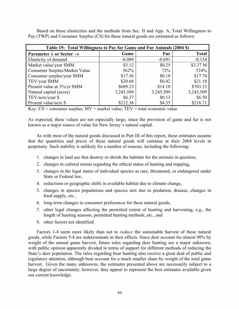
44

Based on these elasticities and the methods from Sec. II and App. A, Total Willingness toPay (TWP) and Consumer Surplus (CS) for these natural goods are estimated as follows:

Table 19: Total Willingness to Pay for Game and Fur Animals (2004 $)Parameter ↓ or Sector → Game Fur TotalElasticity of demand -0.089 -0.691 -0.134Market value/year $MM $3.12 $0.25 $3.37 MConsumer Surplus/Market Value 562% 72% 524%Consumer surplus/year $MM $17.56 $0.18 $17.74TEV/year $MM $20.68 $0.42 $21.10Present value at 3%/yr $MM $689.23 $14.10 $703.33Natural capital (acres) 3,245,509 3,245,509 3,245,509TEV/acre/year $ $6.37 $0.13 $6.50Present value/acre $ $212.36 $4.35 $216.71Key: CS = consumer surplus; MV = market value; TEV = total economic value

As expected, these values are not especially large, since the provision of game and fur is notknown as a major source of value for New Jersey’s natural capital.

As with most of the natural goods discussed in Part III of this report, these estimates assumethat the quantities and prices of these natural goods will continue at their 2004 levels inperpetuity. Such stability is unlikely for a number of reasons, including the following:

1. changes in land use that destroy or shrink the habitats for the animals in question,2. changes in cultural norms regarding the ethical status of hunting and trapping,3. changes in the legal status of individual species as rare, threatened, or endangered under

State or Federal law,4. reductions or geographic shifts in available habitat due to climate change,5. changes in species populations and species mix due to predation, disease, changes in

food supply, etc.,6. long-term changes in consumer preferences for these natural goods,7. other legal changes affecting the permitted extent of hunting and harvesting, e.g., the

length of hunting seasons, permitted hunting methods, etc., and8. other factors not identified.

Factors 1-4 seem more likely than not to reduce the sustainable harvest of these naturalgoods, while Factors 5-8 are indeterminate in their effects. Since deer account for almost 90% byweight of the annual game harvest, future rules regarding deer hunting are a major unknown,with public opinion apparently divided in terms of support for different methods of reducing theState’s deer population. The rules regarding bear hunting also receive a great deal of public andregulatory attention, although bear account for a much smaller share by weight of the total gameharvest. Given the many unknowns, the estimates presented above are necessarily subject to alarge degree of uncertainty; however, they appear to represent the best estimates available givenour current knowledge.

45

Section VII: Non-Farm Plants

As used here, “non-farm plants” includes grasses, wildflowers, herbs, medicinal plants, andother types of plants found in New Jersey, excluding trees, which are considered in SectionVIII.41 The focus here is on the plants themselves considered as ecosystem goods rather than onthe pleasure many people obtain from viewing rare or aesthetically pleasing plants in their nativehabitats; the latter type of aesthetic and recreational benefit is treated in Part II as an ecosystemservice provided by specific landscape types.

Plants obviously play an essential role in sustaining all of New Jersey’s ecosystems.However, that role is not considered separately in this study, since the ecosystems themselves aretreated directly in terms of their production of economically valuable goods and services. Tocount this “ecosystem maintenance” role of plants as a separate source of value would be toengage in double-counting; from the standpoint of economics, this function of plant life is treatedas an “input” to the production of goods and services, which are then valued directly.

Relatively little quantitative information is available on the uses of New Jersey’s non-agricultural plants (other than trees). This contrasts with the considerable attention paid to rare,threatened, and endangered animal species (see, e.g., Niles et al. 2001). 42 However, two of thevalues provided by plants have received attention in the economics literature: 1) the use ofplants for medicinal and pharmaceutical purposes, and 2) the general importance of plants interms of biodiversity and genetic resources. These uses are discussed briefly below.

Medicinal plants are a subject of great interest to some of the economists who work in thearea of ecosystem valuation, especially those who work on tropical rainforest issues. As is wellknown, some of our most important medicines are derived or were first extracted from naturallyoccurring plants, including aspirin, cocaine, and quinine. The value of such compounds, asmeasured by sales, is extremely large in some cases. The problem in estimating the value of thistype of natural capital is our inability to predict where, when, and whether similar discoverieswill be made in the future and, if so, how valuable those discoveries will prove to be.

One study that sought to quantify this pharmaceutical value these is Simpson et al. (1996).That study attempted to determine the private in situ value of the marginal43 species for use inpharmaceutical research and private value of the marginal acre of threatened habitat forpharmaceutical research. Using demand analysis for a limited sample of pharmaceuticalresearchers, the study obtained one-time generic values of $12,040 for the “marginal” speciesand $10 per acre for threatened habitat (values in 2004 $). The researchers sought to explainwhat they viewed as relatively low values by citing the following factors:

41 We can include fungi here, even thought they are no longer considered to be plants.42 In this regard, plant species are covered under the federal Endangered Species Act but not under currentstate law.43 In studies that ascertain values for genetic resources in situ, every “unit” (species or habitat area) ofbiodiversity is viewed as making an equal marginal contribution to the success of the bio-prospectingenterprise; that is, one species or one acre of habitat is about as valuable as any other.

46

• individual redundancy, i.e., if all representatives of a species produce a particularcompound, individuals in excess of the number needed to maintain a viable populationare redundant;

• species redundancy, i.e., instances in which identical drugs, or drugs with similar clinicalproperties, have been isolated from different species; and

• medical redundancy, where different therapeutic mechanisms may be effective in treatingthe same symptoms.

Given these caveats, the results of Simpson et al. (1996) at best provide indications of theorder of magnitude of the benefits. Other studies have pointed to different approaches that couldyield substantially different results. At this point, there is no generally accepted approach ormethodology for assessing biodiversity value, and for this reason, no attempt is made here toestimate the potential pharmaceutical value of New Jersey’s non-agricultural plants.

Plant species can also be considered more generally from the standpoint of biodiversity,although this takes us beyond the narrow focus on ecosystem goods.44 Biodiversity is probablyessential for habitat maintenance, since healthy ecosystems are usually characterized bycontaining a variety of species with population sizes sufficient to ensure long-term viability, allelse being equal, e.g., climate, human development of natural lands, absence of invasive species,etc. Individual species also represent repositories of genetic data that can prove critical forecosystem survival when habitats are subjected to stress from climate change, habitatfragmentation, entrance of invasive species (including disease-causing organisms) into thehabitat, etc.

While biodiversity is unquestionably valuable, the study of the economics of biodiversity isstill in its early stages, and only a few studies have attempted to quantify its value. Given theabsence of data on New Jersey’s endowment of plant species and the lack of a generally acceptedvaluation method, this study does not attempt to estimate a value for the natural capitalrepresented by New Jersey’s non-agricultural plant resources.

The conservation of biodiversity and genetic data is sometimes distinguished from theprotection of rare, threatened, and endangered species. The latter has value in its own right,including the willingness of many people to pay for such protection even if they have never seenthe species in question. However, the evidence for such willingness comes mainly from studiesinvolving animals rather than plants and thus affords very little on which to base an analysis ofNew Jersey’s plant resources. The aesthetic and recreational enjoyment that many people derivefrom viewing such species is considered in Part II as a service provided by the state’secosystems.

44 Some use the term biodiversity to mean the number of species in a given geographic area; others use itto mean the population sizes for the species in that area. These uses are not distinguished in thisdiscussion.

47

Section VIII: Fish and Shellfish

Since they involve different types of data and different valuation issues, the products ofcommercial and recreational fishing will be treated separately below. The natural capital relevantto this class of natural goods is considered to be as follows:

• For commercial fishing, New Jersey’s 299,835 acres of coastal shelf and 455,700 acres ofestuaries and tidal bays, for a total of 755,535 acres.

• For recreational saltwater fishing, the same two marine ecosystems plus 190,520 acres ofsaltwater wetlands, for a total of 946,055 acres.

• For recreational freshwater fishing, 86,232 acres of open fresh water and 181,099 acres ofunforested freshwater wetlands, for a total of 267,331 acres.

Certain wetlands are included in the above to reflect their role as fish nurseries and sources ofbait fish. In effect, these wetlands are grouped in an integrated system with the waters where thefish are actually harvested, and the value of the harvest is allocated pro rata across the entiresystem. Forested freshwater wetlands are not included in these numbers based on the assumptionthat such wetlands are more important for hunting than for fishing.

Commercial Fishing

Fishing (including shellfishing) is an important industry in New Jersey. Six major fishingports are located in the state, including Atlantic City, Barnegat Light, Belford, Cape May, PointPleasant, and Port Norris, with a commercial fleet totaling more than 1,500 vessels andemploying nearly 3,000 fishermen. The state also has 15 seafood processing plants and 81wholesalers employing more than 2,200 workers (NJDA 2005). Recreational fishing is alsosignificant with an estimated 806,000 participants in 2001 according to the U.S. Fish andWildlife Service (USFWS 2003).

Fishery statistics are available from the National Marine Fisheries Service (NMFS) mainlyin terms of commercial fisheries and to a certain extent marine recreational fisheries. Data on thelatter are also compiled periodically by the U.S. Fish and Wildlife Service through its NationalSurvey of Fishing, Hunting and Wildlife-Associated Recreation.

According to NMFS, over 100 species of finfish and shellfish are harvested in the waters offNew Jersey. In 2004, vessels based in New Jersey ports landed over 187 million pounds of fish(finfish and shellfish), valued at almost $146 million paid to fishermen at the dock (the “ex-vessel” price) (NMFS 2005).

The two tables below present information from NMFS on the weight and value for the mostimportant finfish and shellfish species harvested in 2004. The first table presents the 2004finfish data, with species ranked by estimated value:

(see next page for tables)

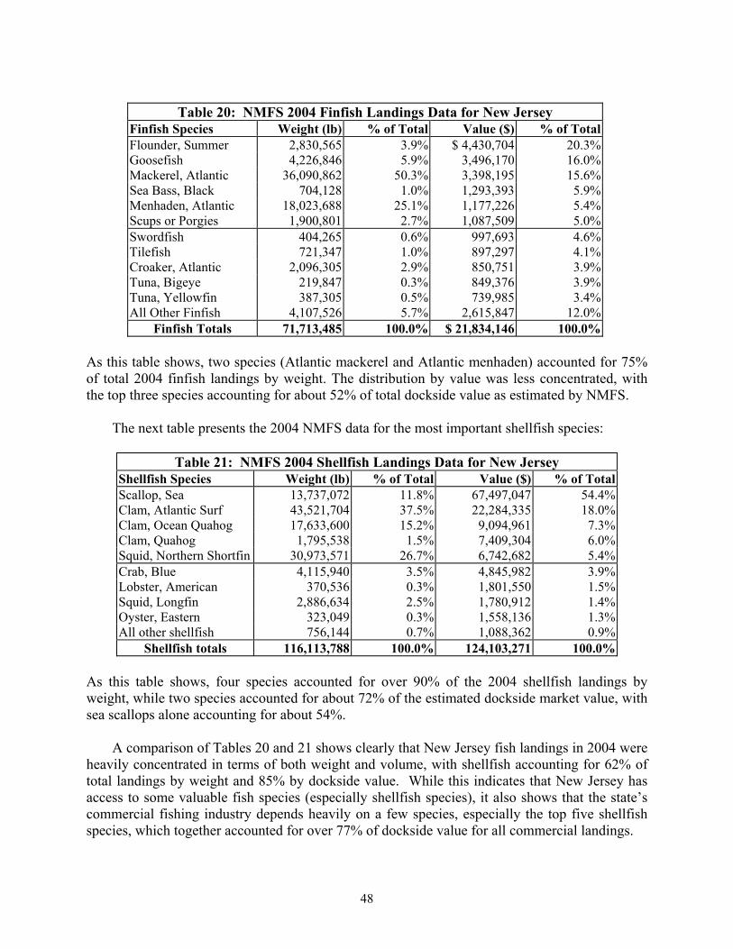
48

Table 20: NMFS 2004 Finfish Landings Data for New JerseyFinfish Species Weight (lb) % of Total Value ($) % of TotalFlounder, Summer 2,830,565 3.9% $ 4,430,704 20.3%Goosefish 4,226,846 5.9% 3,496,170 16.0%Mackerel, Atlantic 36,090,862 50.3% 3,398,195 15.6%Sea Bass, Black 704,128 1.0% 1,293,393 5.9%Menhaden, Atlantic 18,023,688 25.1% 1,177,226 5.4%Scups or Porgies 1,900,801 2.7% 1,087,509 5.0%Swordfish 404,265 0.6% 997,693 4.6%Tilefish 721,347 1.0% 897,297 4.1%Croaker, Atlantic 2,096,305 2.9% 850,751 3.9%Tuna, Bigeye 219,847 0.3% 849,376 3.9%Tuna, Yellowfin 387,305 0.5% 739,985 3.4%All Other Finfish 4,107,526 5.7% 2,615,847 12.0%

Finfish Totals 71,713,485 100.0% $ 21,834,146 100.0%

As this table shows, two species (Atlantic mackerel and Atlantic menhaden) accounted for 75%of total 2004 finfish landings by weight. The distribution by value was less concentrated, withthe top three species accounting for about 52% of total dockside value as estimated by NMFS.

The next table presents the 2004 NMFS data for the most important shellfish species:

Table 21: NMFS 2004 Shellfish Landings Data for New JerseyShellfish Species Weight (lb) % of Total Value ($) % of TotalScallop, Sea 13,737,072 11.8% 67,497,047 54.4%Clam, Atlantic Surf 43,521,704 37.5% 22,284,335 18.0%Clam, Ocean Quahog 17,633,600 15.2% 9,094,961 7.3%Clam, Quahog 1,795,538 1.5% 7,409,304 6.0%Squid, Northern Shortfin 30,973,571 26.7% 6,742,682 5.4%Crab, Blue 4,115,940 3.5% 4,845,982 3.9%Lobster, American 370,536 0.3% 1,801,550 1.5%Squid, Longfin 2,886,634 2.5% 1,780,912 1.4%Oyster, Eastern 323,049 0.3% 1,558,136 1.3%All other shellfish 756,144 0.7% 1,088,362 0.9%

Shellfish totals 116,113,788 100.0% 124,103,271 100.0%

As this table shows, four species accounted for over 90% of the 2004 shellfish landings byweight, while two species accounted for about 72% of the estimated dockside market value, withsea scallops alone accounting for about 54%.

A comparison of Tables 20 and 21 shows clearly that New Jersey fish landings in 2004 wereheavily concentrated in terms of both weight and volume, with shellfish accounting for 62% oftotal landings by weight and 85% by dockside value. While this indicates that New Jersey hasaccess to some valuable fish species (especially shellfish species), it also shows that the state’scommercial fishing industry depends heavily on a few species, especially the top five shellfishspecies, which together accounted for over 77% of dockside value for all commercial landings.

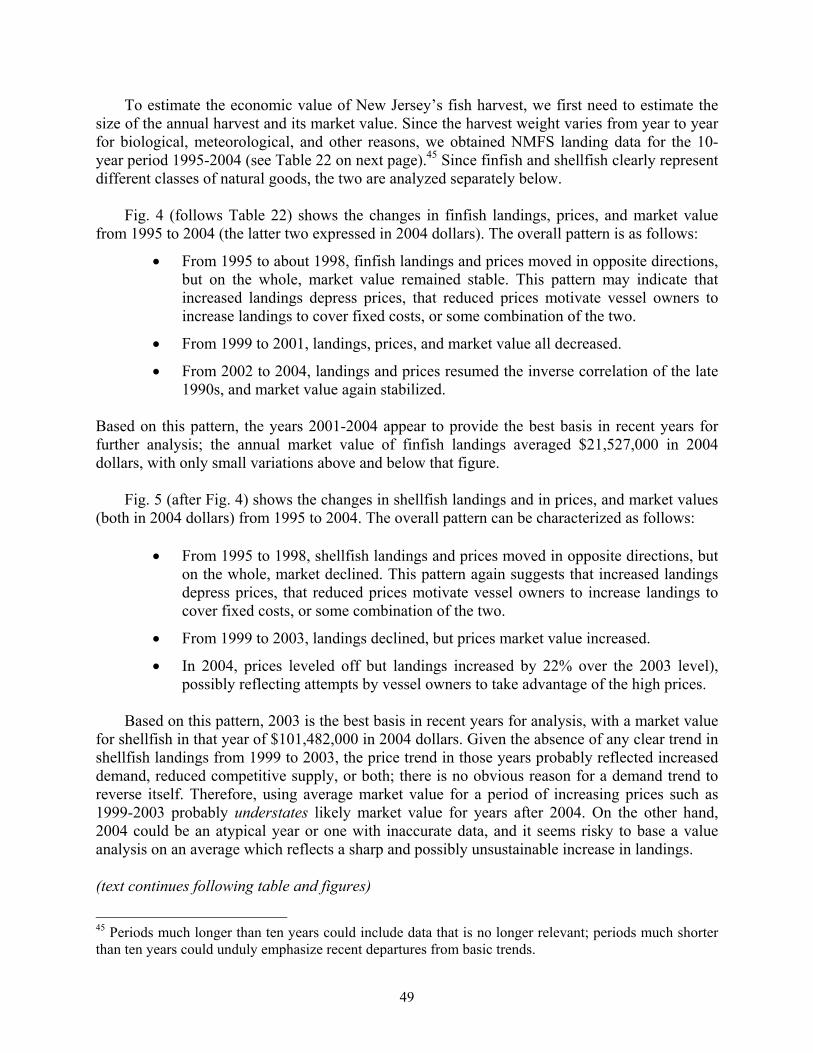
49

To estimate the economic value of New Jersey’s fish harvest, we first need to estimate thesize of the annual harvest and its market value. Since the harvest weight varies from year to yearfor biological, meteorological, and other reasons, we obtained NMFS landing data for the 10-year period 1995-2004 (see Table 22 on next page).45 Since finfish and shellfish clearly representdifferent classes of natural goods, the two are analyzed separately below.

Fig. 4 (follows Table 22) shows the changes in finfish landings, prices, and market valuefrom 1995 to 2004 (the latter two expressed in 2004 dollars). The overall pattern is as follows:

• From 1995 to about 1998, finfish landings and prices moved in opposite directions,but on the whole, market value remained stable. This pattern may indicate thatincreased landings depress prices, that reduced prices motivate vessel owners toincrease landings to cover fixed costs, or some combination of the two.

• From 1999 to 2001, landings, prices, and market value all decreased.

• From 2002 to 2004, landings and prices resumed the inverse correlation of the late1990s, and market value again stabilized.

Based on this pattern, the years 2001-2004 appear to provide the best basis in recent years forfurther analysis; the annual market value of finfish landings averaged $21,527,000 in 2004dollars, with only small variations above and below that figure.

Fig. 5 (after Fig. 4) shows the changes in shellfish landings and in prices, and market values(both in 2004 dollars) from 1995 to 2004. The overall pattern can be characterized as follows:

• From 1995 to 1998, shellfish landings and prices moved in opposite directions, buton the whole, market declined. This pattern again suggests that increased landingsdepress prices, that reduced prices motivate vessel owners to increase landings tocover fixed costs, or some combination of the two.

• From 1999 to 2003, landings declined, but prices market value increased.

• In 2004, prices leveled off but landings increased by 22% over the 2003 level),possibly reflecting attempts by vessel owners to take advantage of the high prices.

Based on this pattern, 2003 is the best basis in recent years for analysis, with a market valuefor shellfish in that year of $101,482,000 in 2004 dollars. Given the absence of any clear trend inshellfish landings from 1999 to 2003, the price trend in those years probably reflected increaseddemand, reduced competitive supply, or both; there is no obvious reason for a demand trend toreverse itself. Therefore, using average market value for a period of increasing prices such as1999-2003 probably understates likely market value for years after 2004. On the other hand,2004 could be an atypical year or one with inaccurate data, and it seems risky to base a valueanalysis on an average which reflects a sharp and possibly unsustainable increase in landings.

(text continues following table and figures)

45 Periods much longer than ten years could include data that is no longer relevant; periods much shorterthan ten years could unduly emphasize recent departures from basic trends.

50

Table 22: New Jersey Commercial Fishery Landings 1995 – 2004

Finfish Price Ex-vessel Shellfish Price Ex-vessel Total Price Ex-vesselYear Wt (000 lb) $/100 lb. value $000 Wt (000 lb) $/100 lb. value $000 Wt (000 lb) $/100 lb. value $0001995 64,755 41.90 27,132 112,131 81.08 90,916 176,886 66.74 118,0481996 79,466 34.29 27,249 103,348 83.94 86,750 182,813 62.36 113,9991997 74,723 42.02 31,399 100,134 85.74 85,855 174,857 67.06 117,2531998 84,221 35.00 29,477 112,922 73.69 83,212 197,143 57.16 112,6891999 76,703 38.80 29,761 91,954 88.31 81,205 168,658 65.79 110,9662000 70,475 35.90 25,301 101,328 91.05 92,259 171,803 68.43 117,5602001 71,141 29.57 21,036 97,400 99.13 96,552 168,541 69.77 117,5892002 65,046 32.20 20,945 97,093 100.32 97,404 162,139 72.99 118,3482003 75,102 29.83 22,403 95,030 106.79 101,482 170,132 72.82 123,8852004 71,107 30.55 21,723 116,073 106.87 124,048 187,180 77.88 145,771

Source: National Marine Fishery Service, US Dept. of Commerce

Note: prices and ex-vessel values are based on conversion of historical dollars to 2004 dollars using the US Bureau of Labor Statistics,All-Items Urban Consumer Price Index (CPI-U), 1982-1984 = 100, not seasonally adjusted.

51

Fig. 4: Commercial Finfish Landings, Price, and Value

0

10,000

20,000

30,000

40,000

50,000

60,000

70,000

80,000

90,000

100,000

1995 1996 1997 1998 1999 2000 2001 2002 2003 2004

000

lbs

or $

000

$0.00

$5.00

$10.00

$15.00

$20.00

$25.00

$30.00

$35.00

$40.00

$45.00

$50.00

2004

$/1

00 lb

s

Landings Value Price

52

Fig. 5: Commercial Shellfish Landings, Price, and Value

20,000

40,000

60,000

80,000

100,000

120,000

140,000

1995 1996 1997 1998 1999 2000 2001 2002 2003 2004

000

lbs

or $

000

$0.00

$20.00

$40.00

$60.00

$80.00

$100.00

$120.00

2004

$/1

00 lb

s

Landings Value Price

53

To summarize, the analysis that follows assumes annual commercial landings with a marketvalue of about $123 million, comprised of 17.5% or $21,527,000 for finfish and 82.5% or$101,482,000 for shellfish (all figures in 2004 dollars). It must be emphasized that these are notforecasts of the sustainable yield for New Jersey’s commercial ocean fisheries but ratherestimates based on historical data. Similarly, the prices implicit in these figures are not based onprojections of future consumer demand or future alternative supplies but reflect actual historicalprices calculated from NMFS data.

Given the heterogeneity of the commercial fish harvest, significant further research wouldbe needed to determine whether species-specific elasticity of demand estimates are available;given the similarities among fish species, the gain in accuracy from such research would notnecessarily be significant. For simplicity, this class of natural goods is analyzed as a singlesource of food, using the US Department of Agriculture’s estimated elasticity of demand for fishof –0.098. Non-food uses of fish products are not addressed.

Based on that elasticity value and on the formulas described in Section II and Appendix A,46

the Total Willingness to Pay (TWP) and Consumer Surplus (CS) for this class of natural goodsare estimated to be as follows:

Table 23: Total Willingness to Pay for Commercial Fish Harvest (2004 $)Parameter ↓ or Sector → Finfish Shellfish TotalElasticity of demand -0.098 -0.098 -0.098Market value/year $MM $21.5 $101.5 $123.0Consumer Surplus/Market Value 510% 510% 510%Consumer surplus/year $MM $109.7 $517.7 $627.3TEV/year $MM $131.2 $619.2 $750.3Present value at 3%/yr $Bn $4.372 $20.638 $25.010Natural capital (acres) 755,535 755,535 755,535TEV/acre/year $ $174 $819 $993Present value/acre $ $5,786 $27,316 $33,102Key: CS = consumer surplus; MV = market value; TEV = total economic value

The above discussions focuses on sales at the docks, i.e., sales from fishing boats towholesale distributors. Subsequent sales to retail fish outlets, restaurants and ultimate consumers 46 An alternative known as the “current rent” method has been widely employed in the construction ofnatural resource asset accounts by the U.S. Bureau of Economic Analysis and other researchers. Thecurrent rent from an additional fish harvested is its contribution to total revenue less the marginal cost ofcatching it and bringing it ashore in salable condition. Using current rents for valuing the entire fish stockessentially means estimating the current liquidation price for the stock. The method has the advantagethat, under certain assumptions, only data on current market prices and costs are needed, i.e., the analystneed not attempt to forecast future market conditions. However, the method requires estimates of currentstock sizes for commercially important species, which are not available for New Jersey. For somerelatively well-understood fisheries, it has been proposed that bioeconomic models be used to assesslikely future stocks, costs of fishing, and net rent under different management regimes. Again, as far as isknown, no such models have been developed for New Jersey’s commercial fish species.

54

will involve other costs and mark-ups, and for that reason, the estimated dockside price affords abetter measure of the value to society of the fish themselves, apart from the processing anddistribution chains that lead to the ultimate consumers.

Based on the assumed market value of the annual harvest, the economic value of NewJersey’s commercial fisheries is clearly substantial. However, that value will be affected bychanges in fish populations, species mix, consumer preferences, competition for supplies withother fishing nations, demand for fish from overseas markets, and other factors. In this regard, itis well-known that many commercially important fish species have been overfished in recentyears to the point where some fisheries are no longer commercially viable. There are powerfulforces working to prolong this trend, including rising incomes in many countries (making itpossible to consume more expensive sources of protein such as fish), fears about the safety ofother protein sources such as beef and poultry, publicity on the health benefits of fishconsumption, improvements in fishing technology, increases in the scale of commercial fishingoperations, etc. Increases in commercial fish farming may be a partially offsetting factor.

It is also becoming apparent that greenhouse gas-induced lake, stream and ocean warmingand acidification and other pollution-related threats to fish and their food supplies (mainlysmaller fish species) now threaten the future commercial viability of an increasing number offisheries, although we are not aware of specific information involving New Jersey fisheries.Since it is inherently difficult for climate models to project conditions for small geographicregions such as the fishing grounds off the New Jersey coast, it may take some time before suchstate-specific information becomes available.

Given all of these uncertainties, the estimated values could reflect overestimates of the likelyvolume and value of future landings. However, in the absence of a peer-reviewed forecastingmethodology for New Jersey, history appears to provide the best basis for a quantitativevaluation of New Jersey’s commercial fish and shellfish resources.

Recreational Fishing

Although it operates at a much smaller scale than commercial fishing, recreational fishingalso provides a source of food that may be important for some households. Data on recreationalfishing is available from NMFS (for saltwater fishing) and from NJDEP’s Division of Fish andWildlife (for freshwater fishing). We consider each of these in turn.

Saltwater fish. The table on the next page shows the 2004 recreational harvest of saltwaterfish for New Jersey and the value of that harvest as estimated by NMFS. According to NMFS,the 2004 harvest had an aggregate weight of 13.7 million pounds and an estimated landing valueof $20.5 million, for an average landing price of $1.49/lb. The many uncertainties make itdifficult to project future landings with any confidence, but in the absence of a bettermethodology and better data, the 2004 value will be taken as a recurring market value for thissub-sector.

55

Table 24: 2004 New Jersey Recreational Saltwater HarvestAFS Species Name Pounds Dollars Price/Lb.Striped Bass* 4,634,160 $ 12,234,182 $ 2.64Flounder, Summer 3,413,126 5,358,608 1.57Bluefish 2,714,608 1,004,405 0.37Croaker, Atlantic 909,009 372,694 0.41Tautog 183,185 351,715 1.92Sea Bass, Black 166,284 305,963 1.84Weakfish 259,722 225,958 0.87Flounder, Winter 136,339 185,421 1.36Mackerel, King And Cero 89,641 170,318 1.90Drum, Black 783,418 109,679 0.14Perch, White 77,620 59,767 0.77Scups Or Porgies 60,111 34,263 0.57Other Tuna/Mackerel 132,525 18,554 0.14Bonito, Atlantic 10,035 17,561 1.75Shark, Dogfish 29,290 11,130 0.38Sea robins 85,642 9,421 0.11Mackerel, Spanish 2,983 5,369 1.80Flounder, Other 959 1,112 1.16Herring 18,503 1,110 0.06Skates 5,893 1,061 0.18Hake, Red 842 497 0.59Other Saltwater Species 1,109 1,652 1.49Total 13,715,004 $ 20,480,440 $ 1.49*price based on 2004 Middle Atlantic totals = NY+DE = $2,436,062/923,034 lbs.Note: does not include inland freshwater harvestsSource: NMFS website accessed 8/15/06 (www.st.nmfs.gov)

It should be noted that the average price for the recreational saltwater finfish47 harvest ismuch higher than the average for the equivalent commercial catch due to a difference in the mixof species. For example, if we limit our attention to the saltwater finfish species harvested bothrecreationally and commercially, the top three recreational species by weight, accounting for78.5% of the 2004 recreational saltwater finfish harvest, are striped bass ($2.64/lb), summerflounder ($1.57/lb), and bluefish ($0.37/lb). In contrast, tuna and Atlantic mackerel, with aweighted average price of $0.14/lb, account for 78.5% of the 2004 commercial saltwater finfishharvest for the same set of species. Based on the mix of these species in the commercial harvest,the average commercial price for all species in this set is $0.35/lb.—a figure that is still wellbelow the 2004 recreational average of $1.49/lb.48 (all prices are in 2004 dollars).

Freshwater fish. The table on the next page shows the 2004 recreational harvest forfreshwater fish, based on a 2003 survey of anglers fishing in New Jersey. An earlier 2001 studyby the US Fish and Wildlife Service estimated total anglers in New Jersey at about 806,000, andthe 2003 study used a sample of 0.1% of that amount or 860 anglers. The 2003 study found that 47 The NMFS recreational harvest data do not include shellfish.48 The average 2004 price for saltwater finfish species harvested commercially but not recreationally waslower still at $0.21/lb.

56

the average angler kept 11.23 fish during the fishing season, which extrapolates to about 9million fish over the total population of 806,000 anglers.

Table 25: New Jersey Recreational Freshwater HarvestSpecies % Sample # Fishers* Avg # kept # Fish keptbrook/brown/rainbow trout 36% 310 9.85 3,050crappie 25% 215 7.74 1,664lake trout 17% 146 9.85 1,440largemouth bass 65% 559 0.63 352striped bass (freshwater) 30% 258 1.33 343channel catfish 15% 129 1.41 182smallmouth bass 46% 396 0.37 146walleye 9% 77 1.34 104pickerel 32% 275 0.25 69northern pike 18% 155 0.36 56striped bass (hybrid) 14% 120 0.34 41other** 25% 215 7.45 1,602

Total or average 100% 806 11.23 9,049

*based on an 0.1% sample of NJ Total # fishers 805,870anglers; includes multiple responses Avg # fish kept/person 11.23

Total # fish kept/yr 9,047,229**bluegill, sunfish, other, Assumed avg value/fish $1.49or no species specified Total value/yr $13,480,371

Sources: New Jersey Anglers' Participation in Fishing, Harvest Success, and Opinionson Fishing Regulations, survey conducted by Responsive Management for theNew Jersey Division of Fish and Wildlife, 2003.

The 2003 study did not estimate the market value of the recreational freshwater catch, andthere appears to be no official source for this information.49 Since the recreational saltwater andfreshwater data are both for finfish only, we have used the average recreational saltwater price of$1.49/lb to estimate the value of the recreational freshwater catch as $13.48 million/yr.Combining this with the saltwater harvest of $20.48 million/yr gives a total market value ofabout $34 million/yr.50

Based on the assumed continuation of these annual harvest levels, the elasticity of demandof –0.098 assumed for the commercially harvested fish, and the formulas described in Section IIand Appendix A, the Total Willingness to Pay (TWP) and Consumer Surplus (CS) for this classof natural goods are estimated to be as follows:

49 NMFS does not report this information, since freshwater fishing is not within its jurisdiction; sourcessuch as the Fulton Fish Market in New York City report prices only for commercially harvested saltwaterspecies. Retail restaurant prices for freshwater species vary widely and reflect cost and profit componentswhose relationship to the value of the raw fish is unknown.50 Because this part of the natural capital report deals solely with ecosystem and abiotic goods, thesefigures do not reflect the value of the recreational services provided by fishing in New Jersey; suchservices were dealt with in Part II of this report on an ecosystem-specific basis.

57

Table 26: Total Willingness to Pay for Recreational Fish Harvest (2004 $)Parameter ↓ or Sector → Saltwater Freshwater TotalElasticity of demand -0.098 -0.098 -0.098Market value/year $MM $20.5 $13.5 $34.0Consumer Surplus/Market Value 510% 510% 510%Consumer surplus/year $MM $104.6 $68.9 $173.4TEV/year $MM $125.1 $82.4 $207.4Present value at 3%/yr $Bn $4.168 $2.745 $6.913Natural capital (acres) 946,055 267,331 1,213,386TEV/acre/year $ $132 $308 $171Present value/acre $ $4,406 $10,268 $5,697Key: CS = consumer surplus; MV = market value; TEV = total economic value

Limitations and caveats similar to those discussed above for commercial fisheries apply tothe recreational fish harvest. Given these unknowns, the estimated economic values presentedabove are necessarily subject to a large degree of uncertainty; however, they appear to representthe best estimates available given our current knowledge.

58

Section IX: Fuelwood and Sawtimber

In this section, we consider two different types of natural goods provided by New Jersey’sforested lands (including forested wetlands): wood used as a fuel, i.e., the combustion of woodand wood wastes to produce energy for space heating, steam heating, process steam, andelectricity generation, and timber used as a material, i.e., the use of timber for construction,manufacturing of plywood and other wood products, manufacturing of paper and paper products,production of furniture, etc. (The use of trees to stock tree nurseries is included in the analysis ofagriculture above.) Fuelwood and timber present different valuation issues and are treatedseparately below.

The natural capital relevant to this section includes 1,465,668 acres of forest (includingwooded farmland) and 633,380 acres of forested freshwater wetland, for a total of 2,129,048acres. Urban greenspace is not considered as available for producing fuelwood or timber, andthere is apparently no information on the forested portion of New Jersey’s saltwater wetlands.Some riparian corridors are also forested, but even without counting that ecosystem, the totalacreage essentially equals the total of 2.132 million acres reported by the U.S. Forest Service inits 1999 inventory of New Jersey’s forests.

Fuelwood

All of the major energy-using sectors in New Jersey except transportation use wood andwood wastes for energy generation:

• The residential sector burns wood for direct space heating.

• The commercial sector uses wood for space heating, and wood, wood-containingmunicipal waste, and landfill gas from decay of wood and other substances for steamheat and electricity generation.

• The industrial sector uses combustible industrial by-products and wood chips forelectricity generation and process steam.

• The electric power sector uses wood, industrial wood waste and related waste gas, andwood-containing municipal waste as cofiring fuels or primary fuels to produceelectricity.

Wood sold or gathered for residential use is normally measured in cords; one cord equals128 cubic feet of wood (4 x 4 x 8 ft.) according to the standard definition.51 Wood used by othersectors is measured in a variety of units, including tons, kilowatt-hours of electricity, and others.Because of the multiplicity and varying definitions of units, wood and wood waste used as fuelare often reported in terms of the energy produced. The usual unit used for this purpose in theUnited States is the British Thermal Unit; one BTU equals approximately 252 calories; onemillion BTU is equivalent to about 293 kilowatt-hours.

51 Non-standard cords equal to 80 or 85 cubic feet are also employed for certain purposes.

59

The US Energy Information Administration (EIA) of the US Department of Energyestimates the energy content of wood and wood waste used as fuel in New Jersey to be about 20million BTU per cord.52 Based on that value, the table below summarizes New Jersey’s use ofwood and wood waste as a fuel in 2003, the most recent year for which such data are available.

TABLE 27: USE OF WOOD AS A FUEL IN NEW JERSEY IN 2003Sector 000 cords Billion BTU Share of totalElectric power 1,025 20,500 62.6%Residential 422 8,440 25.8%Industrial 115 2,300 7.0%Commercial 75 1,500 4.6%

Total* 1,640 32,800 100.0%*detail does not sum to totals due to rounding.

The total of 32.8 trillion BTUs represented about 1.3 % of New Jersey’s energy consumption in2003. The underlying data is collected by EIA from a variety of sources, including the USCensus, other official surveys, reports filed by electricity generators, etc. The informationnecessarily excludes an unknown amount of unreported gathering of fuelwood by individualhomeowners and others for their own use.

The price of fuelwood depends on a variety of factors, including the quality of the wood, thearea where the wood is harvested, transportation costs to the locality where the wood is sold,whether the wood is sold as logs or as wood chips, whether it is sold at wholesale or at retail, etc.In New Jersey, retail prices per cord of firewood sold to residential customers ranged from$150/cord to $230/cord in 2004 (Murray 2004). However, some quoted prices includetransportation to the buyer’s residence and stacking, while others do not; the prices reflect theretailer’s costs, including the cost of transporting the wood from the harvest site to the sale siteand possibly stacking it there.

EIA reported total New Jersey end-user purchases of wood and wood wastes in 2003 of$37.5 million which comes to $22.87/cord based on the consumption shown in Table 27 or$23.48/cord in 2004 dollars.53 This is an average price; residential and commercial customerspaid substantially more, while industrial and electric power users paid substantially less. 54 Asdescribed at length in the discussion of water resources in Section III, the most appropriate figurefor natural capital valuation is the value at the point of harvest or in situ value rather than theretailer’s or end user’s delivered price. However, even EIA’s reported average residential cost of 52 The heat content of wood actually varies from 15 to 20 million BTU per cord depending on the type ofwood, moisture content, method of combustion, and other factors. Using the upper end of this rangeresults in a lower estimate of the number of cords used in New Jersey and is therefore conservative fromthe standpoint of natural capital valuation.53 This calculation includes 1.35 million cords with an average 2003 cost of $27.80/cord and 290,000cords of what EIA calls “uncosted” fuel with an assumed cost of zero.54 This may reflect in part the fact that the fuelwood used by residential and commercial customers tendsto be in the form of small logs, while industrial and utility users tend to use wood chips and other woodwastes.

60

$44.08/cord is so far below actual New Jersey retail firewood prices that it clearly represents avalue at or close to the point of harvest; therefore, EIA’s overall average of $23.48/cord in 2004dollars will be used to as the market value per cord in this analysis.

It should be noted that EIA does not publish information on the geographic source(s) offuelwood used in New Jersey, and no other source has been found for this data. Therefore, thereis no way of determining what portion (if any) of New Jersey’s total fuelwood usage representswood imported into New Jersey. In the absence of other information, the analysis below assumesthat 100% of the wood used in New Jersey comes from in-state sources.

The elasticity of demand for fuelwood has been found to vary by type of end user (Skog2003), as the next table indicates:

Table 28: New Jersey Fuelwood Consumption in 2003(based on 20 MMBtu/cord)

Sector 000 Cords* Shares Elasticity WeightedResidential 422 25.8% -0.87 -0.224Commercial 75 4.6% -0.15 -0.007Industrial 115 7.0% -0.39 -0.027Electric power 1,025 62.6% -0.13 -0.081

Total 1,640 100.0% -0.340*details do not sum to total due to rounding.

If we weight each sector’s elasticity by that sector’s share of total New Jersey consumption, weobtain an average elasticity of -0.340.

Based on the above, we can estimate the value of New Jersey’s fuelwood as follows:

Table 29: Total Willingness to Pay for Fuelwood (2004 $)Parameter ValueKey assumptions:Pct. of fuelwood from NJ 100%Elasticity of demand -0.340Total NJ supply (000 cords/year) 1,640Market value per cord (2004 $) $23.48Market value/year $MM $38.507Consumer Surplus/Market Value 147%Consumer surplus/year $MM $56.606TEV/year $MM $95.112Present value at 3%/yr $Bn $3.170Natural capital (acres) 2,129,048TEV/acre/year $ $45Present value/acre $ $1,489

Key: CS = consumer surplus; MV = market value; TEV = total economic value

61

The estimated annual value of $58.7 million is based on the assumption that future consumptionwill remain constant at the 2003 level reported by EIA, which in turn implies that this level is themaximum that is both ecologically sustainable and economically feasible.

As with the other goods provided by New Jersey’s natural capital, the continued provision ofthis level of benefits depends on climate, land use patterns, energy consumption, fuel preferencesamong energy users, the mix of end-user sectors, etc. None of these factors can be predicted withmuch confidence, and the valuation presented above arguably represents the best estimate thatcan be derived given the available data.

Sawtimber

The other main category of wood resources in New Jersey is sawtimber, i.e., timber intendedfor use in furniture, home-building, etc. Sawtimber consists of trees that are larger than thoseharvested for fuelwood; unlike fuelwood, sawtimber does not include standing and fallen deadtrees or wood wastes. Cubic foot for cubic foot, the value of wood as a construction andmanufacturing material is much greater than its value as fuel.

Forests and forested wetlands cover about 2.1 million acres or 45% of New Jersey’s totalland area, a remarkable figure for a state that has experienced substantial population growth andeconomic development since World War II. About 1.9 million acres or 90% of the 2.1 millionacres are classified by the United States Forest Service (USFS) as “timberland”, i.e., forestedland containing resources suitable for commercial timber harvesting under a regime of sustainedyield management. The other 10% (referred to as Other Forestland) consists of preserved landswhere timber harvesting is administratively restricted and unproductive forests where timberharvesting is economically impractical. Most Other Forestland is publicly owned.

Forests contain a wide variety of trees, including live trees of various species, ages, andsizes, standing and fallen dead trees, etc. Commercial interest focuses on live trees (“growingstock”) that meet certain standards of size and wood quality (“sawtimber”)55. At its simplest, themonetary value of the timber contained in the state’s forests equals the volume of merchantable(commercially valuable) sawtimber times the price per unit volume. (Appendix D describesseveral other timber valuation methods.) Sawtimber volume is conventionally measured inboard-feet; a sawtimber log measuring 1 foot x 1 foot x 1 inch contains 1 board-foot of wood.Since timber prices vary by tree species, the volume data used in valuation must reflect the mixof tree species or forest types in New Jersey’s forests.56

The principal sources of detailed information on New Jersey’s forest resources are theperiodic inventories conducted by USFS; the most recent such inventories took place in 1987 and1999. According to these inventories, the volume of sawtimber on New Jersey’s timberlandincreased from 5.6 billion board-feet in 1987 to 8.1 billion in 1999, an increase of 2.4 billion or 55 In addition to growing stock, topwood (wood and bark of above merchantable height), cull (rotten orrough trees) and non-growing stock may also have commercial value. Due to lack of data, these valuesare not estimated here.56 A “forest type” contains multiple species found growing in close proximity; a “forest type group”include several forest types.

62

43.6%. The average annual increase of 204 million bd-ft/year, if continued through 2004, wouldresult in a sawtimber inventory of 9.1 billion bd-ft in that year. Table 30 on the next pagepresents a detailed breakdown of the above totals.

Table 30 also shows the 2004 stumpage prices (in 2004 dollars per 1,000 board-feet) for thetree species present in New Jersey. Those prices were obtained from a variety of sources sinceno single source had prices for all of the species present in New Jersey; New Jersey itselfapparently has no published source for stumpage prices. Where several states reported pricedata, preference was given to the states closest to New Jersey; as a result, about two-thirds of theprices are from Pennsylvania or other Northeastern states.

Based on the 2004 prices, Table 30 presents an estimated value for the assumed annualincrease in New Jersey’s sawtimber inventory of about $49 million/year. It should beemphasized that this figure does not necessarily represent the value of the sustainable sawtimberyield from New Jersey’s timberland. The estimate is simply based on an annual yield of about204 million-board feet, obtained by dividing the total increase in estimated sawtimber volume of2.4 billion bd-ft from 1987 to 1999 by twelve.57

It can be argued that 204 million bd-ft/yr overstates the sustainable yield because of NewJersey’s loss of forests and forested wetlands to development. However, such losses may bebalanced in part by growth of existing trees, increases in the number of trees per acre (asoccurred from 1987 to 1999), and reforestation of abandoned agricultural land. Moreover, while204 million bd-ft represented 3.6% of the 1987 sawtimber inventory, it represents 2.5% of the1999 inventory and only 2.2% of the projected 2004 inventory. For these reasons, this studydoes not include an acreage adjustment.

A number of empirical studies provide estimates of the elasticity of demand for sawtimberand related products (see Exhibit C). The estimates span a fairly wide range, reflecting themultiple uses of timber; in effect, there are multiple timber markets and multiple elasticities ofdemand. Therefore, Table 31 (following Table 30) uses both the first and third quartiles and themedian to develop a range of estimated valuations.

(text continues after tables)

57 According to the New Jersey Forest Service, only 4.7 million board-feet were harvested on privately-owned timberland during the period from July 2003 to June 2004, based on unaudited reports submittedby certified consulting foresters. If the figure of 4.7 million bd-ft is representative of other years, it isclear that private landowners, who owned 69% of New Jersey’s timberland in 1999, have been harvestingfar less than the average annual increase reported by USFS; the reasons for this difference are notobvious.

63

Table 30: Estimated Value of New Jersey's Sawtimber1987 1999 Net Change Annual Projected Stumpage Source of Value of Value of

Volume Volume in Volume Change 2004 Vol. Price '04 Prices Ann. Chge. '04 StockTree Species MM bd-ft MM bd-ft MM bd-ft MM bd-ft/yr MM bd-ft $/000 bd-ft (state) MM $/yr MM $Atlantic White Cedar 145.1 236.2 91.1 7.6 274.2 $445 AL $3.4 $122.0Shortleaf Pine 72.5 36.8 -35.7 -3.0 21.9 $326 MD/DE -$1.0 $7.1Pitch Pine 722.9 928.9 206.0 17.2 1,014.7 $86 various $1.5 $87.3Virginia Pine 13.3 47.1 33.8 2.8 61.2 $86 various $0.2 $5.3Other Pine 89.3 41.0 -48.3 -4.0 20.9 $88 PA -$0.4 $1.8Eastern Red Cedar 32.3 51.2 18.9 1.6 59.1 $61 ME $0.1 $3.6

Softwood Total 1,075.4 1,341.2 265.8 22.2 1,452.0 $3.9 $227.1Red Maple 441.8 861.2 419.4 35.0 1,036.0 $199 PA $7.0 $206.2Sugar Maple 104.8 116.4 11.6 1.0 121.2 $508 PA $0.5 $61.6Hickory 119.5 254.7 135.2 11.3 311.0 $71 NY $0.8 $22.1Beech 121.6 163.7 42.1 3.5 181.2 $39 NY $0.1 $7.1Ash 406.9 553.9 147.0 12.3 615.2 $252 PA $3.1 $155.0Sweetgum 292.7 412.3 119.6 10.0 462.1 $84 IL $0.8 $38.8Yellow Poplar 646.8 1,066.4 419.6 35.0 1,241.2 $223 PA $7.8 $276.8Blackgum 78.5 100.6 22.1 1.8 109.8 $152 PA $0.3 $16.7Black Cherry 16.2 44.0 27.8 2.3 55.6 $1,143 PA $2.6 $63.5Select White Oaks 403.1 495.7 92.6 7.7 534.3 $270 PA $2.1 $144.3Select Red Oaks 524.6 836.2 311.6 26.0 966.0 $533 PA $13.8 $514.9Other Red Oaks 690.3 866.8 176.5 14.7 940.3 $158 IL $2.3 $148.6Other White Oaks 334.2 432.1 97.9 8.2 472.9 $217 various $1.8 $102.6Other Hardwoods 355.5 512.1 156.6 13.1 577.4 $152 PA $2.0 $87.8

Hardwood Total 4,536.5 6,716.1 2,179.6 181.6 7,624.3 $45.0 $1,845.8

GRAND TOTAL 5,611.9 8,057.3 2,445.4 203.8 9,076.2 $48.9 $2,073.0Source of 1987 and 1999 volume data: USDA Forest Service, 2001, Forest Statistics for New Jersey: 1987 and 1999, Northeastern ResearchStation Resource Bulletin NE-152. Projected 2004 volume = 1999 volume + 5 x avg. increase/yr. from 1987 to 1999.Note 1: Sawtimber is commercial-grade timber that meets minimum size criteria for diameter at breast height (dbh); the minimums are 9 in. dbhfor softwoods and 11 in. dbh for hardwoods. Breast height is defined as 4.5 ft. above ground level.Note 2: The board-foot is a unit of lumber measurement equal to the amount of wood in a sawtimber log 1 ft. long, 1 ft. wide, and 1 in. thick.Note 3: The stumpage price is the price landowners receive from loggers for the right to cut down standing trees. The prices are intended to serveas a general guide for the marketing of standing timber; the actual value of a specific stand of timber depends on timber quality etc.

64

Table 31: Total Willingness to Pay for Sawtimber (2004 $)Parameter ↓ or Estimate → Low-end Central High-endKey assumptions:Elasticity of demand -0.520 -0.250 -0.100Total annual supply (MM bd-ft) 203.783 203.783 203.783Avg. price ($/000 bd-ft) $240 $240 $240Market value/year $MM $48.9 $48.9 $48.9Consumer Surplus/Market Value 96% 200% 500%Consumer surplus/year $000 $46.9 $97.8 $244.5TEV/year $000 $95.8 $146.7 $293.4Present value at 3%/yr $Bn $3.195 $4.890 $9.780Natural capital (acres) 2,129,048 2,129,048 2,129,048TEV/acre/year $ $45 $69 $138Present value/acre $ $1,501 $2,297 $4,594

Key: CS = consumer surplus; MV = market value; TEV = total economic value

A more precise estimate of New Jersey’s sustainable sawtimber yield and value wouldrequire more detailed modeling by tree species of such factors as growth of previouslyestablished trees, colonization of new acreage, deliberate tree plantings and removals, treediseases, normal tree mortality, and other factors. Those variables are in turn affected by suchthings as climate change, spread of disease vectors, crowding-induced tree morbidity andmortality, etc. Such modeling would require an ecological analysis which is beyond the scope ofthis study.

As with all of the other natural capital value estimates presented in this report, these figuresare subject to change as a result of changes in land use (e.g., conversion of forested land toresidential and commercial uses and reforestation of abandoned farmland), climate, tree diseasepatterns, timber harvest policies, the relative prices of different tree species, and numerous otherfactors. The above estimates reflect a snapshot at a point in time; their future relevance willdepend on a combination of human decisions and natural forces. As of 2004, however, NewJersey’s forests clearly made a significant contribution to the state’s collective income andwealth.

65

Section X: Summary and Conclusions

Table 32 below and the tables on the following pages summarize the conclusions reached inthis study of New Jersey’s ecosystem and abiotic natural goods. Based on those results, thisreport concludes that the natural goods provided by New Jersey’s natural capital have economicvalues of about $5.9 billion on an annual basis; the natural capital that provides those goods has apresent value of about $196billion.

As the various tables show, farm goods and fish have the highest shares of these totals,followed by minerals and water; wood and non-farm animals have the lowest shares, and thevalue of non-farm plants cannot be estimated. All of these estimates are subject to variousuncertainties as described throughout this report.

The value provided varies by ecosystem, depending on the types of natural goods provided,the total acreage of the ecosystem, and the average value per acre. Farmland and marineecosystems generate the highest values in terms of total value, followed by barren land (whichincludes mines and quarries), forests, and freshwater wetlands. In terms of value per acre, barrenland ranks first, followed by farmland, marine ecosystems, and open fresh waters.

As emphasized in Section II, total economic value has two components: market value andconsumer surplus. The relative contribution of each to TEV depends on the type of good inquestion, as the following table shows:

Table 32: Components of Total Economic Value(middle estimates; MM 2004 $)

Natural Good MV CS TEV Share CS/TEVFarm products $448 $3,228 $3,676 62.7% 88%Fish (total)* 157 801 958 16.3% 84%Minerals 321 266 587 10.0% 45%Raw water 169 211 381 6.5% 56%Sawtimber 49 98 147 2.5% 67%Fuelwood 39 57 95 1.6% 60%Game/fur animals 3 18 21 0.4% 84%

Total or avg. $1,186 $4,679 $5,864 100.0% 80%Commercial fish 123 627 750 12.8% 84%Recreational fish 34 173 207 3.5% 84%Key: TEV = total economic value; MV = market value; CS = consumer surplus.

The final column in Table 32 gives the Consumer Surplus share of Total Economic Value.The variations among classes of goods reflects the varying estimates of elasticity of demand asobtained from prior empirical studies or official sources. For the reasons described in AppendixA (use of linear rather than constant elasticity; assignment of estimated elasticity to right end ofdemand curve), the above estimates of consumer surplus are more likely to be conservative (i.e.,low) than aggressive.

(text continues after tables)

66

Table 33: Economic Value of New Jersey's Natural Goods(middle estimates; 2004 $)

Middle Estimates

AnnualMarket

Value $MM

AnnualConsumer

Surplus $MM

Total EconomicValue per year

$MM

PresentValue$Bn**

Farm products* $448 $3,228 $3,676 $122.5Minerals 321 266 587 19.6Raw water 169 211 381 12.7Sawtimber 49 98 147 4.9

Subtotal 987 3,804 4,791 159.7Commercial fish 123 627 750 25.0Recreational fish 34 173 207 6.9Fuelwood 39 57 95 3.2Game/fur animals 3 18 21 0.7

Total 1,185 4,679 5,864 195.5Low-end totals 820 1,979 2,798 93.3High-end totals 1,555 8,098 9,652 321.7

*middle estimate = low-end estimate + 50% of the difference between the high and low estimates (see Section V).**present value at 3% per year in perpetuity.

Low-End Estimates:Farm products $108 $778 $885 $29.5Minerals 321 161 481 16.0Raw water 143 119 262 8.7Sawtimber 49 47 96 3.2

Total 621 1,104 1,724 57.5

High-End Estimates:Farm products $787 $5,679 $6,647 $215.6Minerals 321 802 1,123 37.4Raw water 199 497 695 23.2Sawtimber 49 245 293 9.8

Total 1,356 7,223 8,579 285.9

68

Table 34: Annual Value of New Jersey's Natural Capital by Ecosystem (2004 $MM/year) (middle estimate)

EcosystemArea

(acres)FarmGoods

Fish- All*

Minerals- All

RawWater

Wood- All

Game+ Fur

TEV/yr$Mm

TEV/yr$/ac

PV TEV$Bn

PV TEV$/ac

Farmland1 673,464 3,676 79 $3,760 $5,583 $125.3 $186,095Marine2 755,535 850 850 1,125 28.3 37.512Barren land 51,796 587 587 11,337 19.6 377,893Forest land** 1,465,668 173 166 12 349 238 11.6 7,934Freshwater wetland3 814,479 14 96 75 7 191 234 6.4 7,801Open fresh water 86,232 69 10 1 79 921 2.6 30,698Saltwater wetland 190,520 25 2 26 139 0.9 4,617Urban4 1,483,496 20 20 13 0.7 450Riparian buffer 15,146 2 2 118 0.1 3,934Beach/dune 7,837 0 0 0.0 0

TOTAL 5,544,173 3,676 $958 $587 $381 $242 $21 $5,864 $1,058 $195.5 $35,259

1. Farmland:Cropland 546,261 3,223 64 3,291 6,025 109.7 200,828Pasture/grassland 127,203 453 15 469 3,685 15.6 122,8272. Marine:Estuary/tidal bay 455,700 513 513 1,125 17.1 37,505Coastal shelf 299,835 338 338 1,126 11.3 37,5243. Freshwater wetland:Forested 633,380 75 75 5 154 244 5.1 8,122Other 181,099 14 21 1 36 200 1.2 6,6794. Urban:Urban (impervious) 1,313,946Urban green space 169,550 20 20 118 0.7 3,934

*recreational saltwater fishing includes saltwater wetlands; recreational freshwater fishing includes unforested freshwater wetlands.**includes wooded farmland.

69

Table 35: Annual Value of New Jersey's Natural Capital by Ecosystem (2004 $MM/year) (low and high-end estimates)Low-End High-End

Ecosystem Area (acres) TEV/yr$Mm

TEV/yr$/ac

PV TEV$Bn

PV TEV$/ac

TEV/yr$Mm

TEV/yr$/ac

PV TEV$Bn

PV TEV$/ac

Farmland 673,464 $944 $1,402 $31.48 $46,746Marine 755,535 850 1,125 28.34 37,512 850 1,125 28.34 37,512Barren 51,796 481 9,294 16.05 309,805 1,123 21,685 37.44 722,836Forest 1,465,668 260 177 8.66 5,910 593 404 19.76 13,483Freshwater wetland 814,479 145 178 4.82 5,923 316 388 10.53 12,927Open fresh water 86,232 76 884 2.54 29,470 88 1,019 2.93 33,951Saltwater wetland 190,520 26 139 0.88 4,617 26 139 0.88 4,617Urban 1,483,496 14 9 0.46 309 37 25 1.22 821Riparian buffer 15,146 1 81 0.04 2,706 3 216 0.11 7,188Beach/dune 7,837 0 0 0.00 0 0 0 0.00 0

TOTAL 5,544,173 $2,798 $505 $93.28 $16,824 $9,652 $1,741 $321.75 $58,033

*TEV = total economic value

70

Limitations of the Study

The future flows of these natural goods are impossible to predict with confidence becausethey depend heavily on “natural” factors such as climate change and on social policies such asland use conversion that are themselves impossible to project with much precision. Despite thehigh level of uncertainty, however, it seems likely that these factors will tend to operate overtime so as to decrease the value of the goods-producing natural capital in New Jersey.

Two other limitations on the results of this study need to be mentioned. First, totalwillingness to pay (i.e., total economic value) differs from net willingness to pay (net economicvalue). The difference is the cost of producing the goods in question and bringing them tomarket, i.e., to the consumer. Even though nature (conceived of as natural capital) provides thegoods we are discussing, human effort and physical capital (tools, equipment, vehicles, roads,etc.) are required for the goods to actually be used. The net benefit to society is therefore thetotal benefit (or total WTP) minus the costs of production and distribution.

While cost information is thus essential to determining net economic value, market prices donot clearly indicate costs. What they show is the amount actually paid for something. Thatamount in turn consists of the producer’s or supplier’s costs and his or her return or profit,termed producer surplus (see Sec. II). The net benefit to society equals consumer surplus plusproducer surplus. By including producer costs, market values thus overstate the net benefits tosociety.

To estimate producer costs for each natural good so that we can deduct them from totaleconomic value to obtain net economic value would require detailed investigations of each of theindustries involved—mining, fishing, logging, etc.—and such investigations are beyond thescope of this report. In this respect, the estimated values of natural goods summarized above arecomparable to the estimated values of ecosystem services presented in Part II in that they are“gross” (before costs) rather than net.

There is another factor, however, that offsets this overstatement to some extent. When costsare incurred to produce and distribute natural goods (or when costs are avoided because naturalecosystem services eliminate the need for investment in artificial substitutes), the expendituresmade on the natural goods (or the expenditures made with the funds saved on replacing naturalecoservices) stimulate “secondary” economic activity, e.g., as when farmers purchase supplies orequipment or when employees of mining companies spend their wages on goods and services. Inregional economics and macroeconomics, this stimulation of secondary activity is known as the“multiplier effect”.

While secondary activities can result in economic benefits to society that may partiallycompensate for the fact that market values include producer costs, it is beyond the scope of thisreport to analyze the secondary benefits to New Jersey related to each of the industries involvedin producing and distributing natural goods. As a result, the “total” economic values derived inthis report thus represent only the total direct values and therefore understate the true value bythe amount of the secondary benefits.

71

Directions for Future Research

Whether producer costs are completely offset by the unquantified secondary benefits is anempirical matter, and the answer may differ from industry to industry, e.g., from agriculture tologging to mining to fishing. 58 Nonetheless, given the available data and other constraints, total(direct) willingness to pay, defined as Market Value + Consumer Surplus, is a valid, albeitincomplete, first-order approximation of the true economic value of the natural goods producedin New Jersey.

Future research in the following areas could help improve the accuracy and precision of theestimates in this report:

• All ecosystems: more current land use/land cover data.• All ecosystems: relationships between production of services and goods.• Water: more current data on supplies and leakage rates.• Minerals: tonnage and market value of sand dredged offshore.• Farm products: more recent data on the amount of farmland by type.• Fish: prices for recreational freshwater species; role of wetlands.• Non-farm plants: data and methods for preparing rough valuations.• Fuelwood: share of wood harvested in-state; estimated sustainable yield.• Timber: more current annual growth data; estimates of sustainable yield.• All natural goods: further research on relative per-acre ecosystem productivity.• All natural goods: further research on elasticity of demand.

Within the limits imposed by nature, New Jersey has a measure of control over the futurecapacity of its natural capital to produce valuable natural goods. To the extent of that control, thequantities of those goods available in the future should be a matter for informed and deliberatepublic choice. In combination with the findings in Part II on ecosystem services, this reportdocuments the considerable economic value provided by New Jersey’s ecosystems and therebyhelps provide a more scientific basis for those decisions.

58 In most situations, the offset is probably only partial because a dollar’s worth of spending by NewJersey producers will usually generate less than a dollar of secondary activity in the state. This is so forseveral reasons, including the fact that some of the spending flows to out-of-state suppliers (e.g.,manufacturers of farm implements and mining equipment); the same is true when employees spend theirincome on goods produced out-of-state. In addition, unless the suppliers were operating below capacityand unless the employees were otherwise unemployed or underemployed, the secondary activity merelydisplaces other New Jersey activity that would have occurred anyway. Only the net secondary effectsrepresent real contributions to the Net Benefit to New Jersey from producing natural goods.

72

Appendix A: Estimation of Total Economic Value

This appendix presents the derivation of the formula used to obtain the estimates ofConsumer Surplus (CS) and Total Economic Value (TEV) presented in Sections III-VIII. Thederivation of the valuation formula is general and does not depend on the type of natural goodbeing analyzed. The only required input data are the Market Value (MV) of the good when thequantity demanded equals 100% of the annual output and an estimate of the price elasticity ofdemand for that good obtained from the economics literature or official sources.

As suggested in Figures 1-2, Sec. II, determining CS is tantamount to estimating the totalarea TEV between the demand curve59 and the horizontal axis and then subtracting MV from thattotal. To estimate that area, we need to know three things:

• the functional form, i.e., the general shape of the demand curve;

• the slope of the curve, i.e., its relative “steepness”; and

• the y-intercept or asymptote, i.e., the values the demand curve takes on as it approachesand reaches the y-axis (i.e., the vertical axis).

for the range from Q0 to Q1 (see Fig. 1 of Section II).

In general, these factors can be derived in two ways: empirically and analytically. In anempirical study, the investigator has multiple data points available, either from existing databasesor from an original study, e.g. a stated preference study (in essence, a sophisticated consumersurvey in which respondents state how much they would be willing to pay for a given goodunder various circumstances). Using various econometric (i.e., statistical) techniques, theinvestigator can determine the functional form that appears (with varying degrees of certainty) tofit the data most closely.

In our case, we have only one known data point, namely the point where Q = Q1 = 100% ofannual output and P = MP = the average market price of that output, e.g., dollars per thousandgallons of water. (For various technical reasons, values of Q and P from prior years are not asuitable basis for this type of empirical study.) Given this lack of data, we need to turn to a moreanalytic approach. In developing such an approach, we will need to make use of information onthe elasticity of demand for each type of natural good being considered60, and that concept isdiscussed next.

59 In Figs. 1-2, the horizontal axis represents quantity (demand) and the vertical axis represents price,suggesting that price is being graphed as a function of quantity. In fact, the concept of elasticity on whichcritical parts of this analysis are based defines quantity (demand) as a function of price; however, it isstandard practice in economics to show the independent variable price on the vertical axis and thedependent variable quantity on the horizontal. For convenience, we ignore these details and refer simplyto the demand curve. The line defined by the demand function is traditionally termed the demand “curve”even if it is in fact a straight line.60 More precisely, the type of elasticity we will use is the own-price short-run price elasticity of demand.There are also “cross-price”, long-run, income, and supply elasticities.

73

Elasticity of Demand

Elasticity of demand is the percentage change in the quantity demanded associated with aone percent change in price: E = (∆Q/Q) / (∆P/P). For example, if price increases by 1% anddemand falls by 0.5%, the elasticity of demand equals –0.5% / +1% = –0.5. As the exampleshows, elasticities are unit-less numbers because they are the ratio of two percentages; the minussign indicates that price and demand move in opposite directions, as we would expect for typicalgoods like those we are considering.

Estimates of elasticity derived from prior studies are available for each of the broad classesof natural goods analyzed in this report. Those elasticities represent point estimates (i.e., singlevalues) for the types of natural goods being considered, e.g., -0.098 for fish. Technically, a pointestimate applies only to the relatively small portion of the demand curve covered by the originalempirical study; since we are interested in the economic value represented by the entire areaunder that curve, we theoretically need separate estimates of elasticity all along the demandcurve.

It is rarely if ever feasible to obtain such comprehensive information on elasticities.However, as will be demonstrated below, elasticity is a critical variable because if its value isknown, a demand function can be derived, making it possible to estimate CS and TEV. In theabsence of detailed information on the relevant elasticities and the appropriate demand functionfor a given situation, economists often make simplifying assumptions, of which the following areprobably the most common (Nicholson 2002):

• One common assumption is that elasticity is constant all along the demand curve. Thisassumption leads to a type of non-linear demand function discussed below.

• Another common assumption is that the demand function is linear. As will be seen below,this assumption leads to varying elasticities along the demand curve, but those elasticitiescan easily be calculated.

These two approaches are discussed below; for reasons that will be indicated, linear demandfunctions were chosen for this study.

Non-Linear Demand Functions

As just noted, economists often assume for convenience that elasticity is constant at everypoint on the demand curve. The demand functions associated with constant elasticity are non-linear functions of the form Q = A x PE, where Q, P, and E represent respectively quantity, price,and elasticity, and A is an empirically-derived parameter. Fig. 6 shows an example of such afunction, and Nicholson (2002) presents a more detailed discussion of constant elasticity demandfunctions. Such demand functions have been used extensively in the field of water economics,e.g., in Young (2005) and other sources cited in the References.

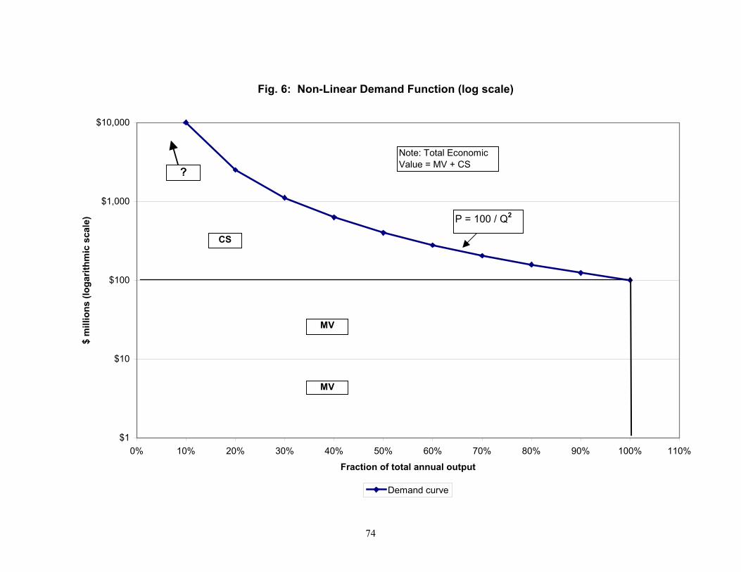
74

Fig. 6: Non-Linear Demand Function (log scale)

$1

$10

$100

$1,000

$10,000

0% 10% 20% 30% 40% 50% 60% 70% 80% 90% 100% 110%

Fraction of total annual output

$ m

illio

ns (l

ogar

ithm

ic s

cale

)

Demand curve

MV

MV

CS

?

P = 100 / Q2

Note: Total Economic Value = MV + CS

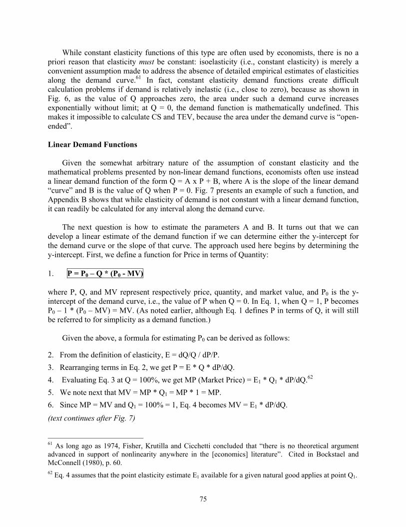
75

While constant elasticity functions of this type are often used by economists, there is no apriori reason that elasticity must be constant: isoelasticity (i.e., constant elasticity) is merely aconvenient assumption made to address the absence of detailed empirical estimates of elasticitiesalong the demand curve.61 In fact, constant elasticity demand functions create difficultcalculation problems if demand is relatively inelastic (i.e., close to zero), because as shown inFig. 6, as the value of Q approaches zero, the area under such a demand curve increasesexponentially without limit; at Q = 0, the demand function is mathematically undefined. Thismakes it impossible to calculate CS and TEV, because the area under the demand curve is “open-ended”.

Linear Demand Functions

Given the somewhat arbitrary nature of the assumption of constant elasticity and themathematical problems presented by non-linear demand functions, economists often use insteada linear demand function of the form Q = A x P + B, where A is the slope of the linear demand“curve” and B is the value of Q when P = 0. Fig. 7 presents an example of such a function, andAppendix B shows that while elasticity of demand is not constant with a linear demand function,it can readily be calculated for any interval along the demand curve.

The next question is how to estimate the parameters A and B. It turns out that we candevelop a linear estimate of the demand function if we can determine either the y-intercept forthe demand curve or the slope of that curve. The approach used here begins by determining they-intercept. First, we define a function for Price in terms of Quantity:

1. P = P0 – Q * (P0 - MV)

where P, Q, and MV represent respectively price, quantity, and market value, and P0 is the y-intercept of the demand curve, i.e., the value of P when Q = 0. In Eq. 1, when Q = 1, P becomesP0 – 1 * (P0 – MV) = MV. (As noted earlier, although Eq. 1 defines P in terms of Q, it will stillbe referred to for simplicity as a demand function.)

Given the above, a formula for estimating P0 can be derived as follows:

2. From the definition of elasticity, E = dQ/Q / dP/P.3. Rearranging terms in Eq. 2, we get P = E * Q * dP/dQ.4. Evaluating Eq. 3 at Q = 100%, we get MP (Market Price) = E1 * Q1 * dP/dQ.62

5. We note next that MV = MP * Q1 = MP * 1 = MP.6. Since MP = MV and Q1 = 100% = 1, Eq. 4 becomes MV = E1 * dP/dQ.

(text continues after Fig. 7)

61 As long ago as 1974, Fisher, Krutilla and Cicchetti concluded that “there is no theoretical argumentadvanced in support of nonlinearity anywhere in the [economics] literature”. Cited in Bockstael andMcConnell (1980), p. 60.62 Eq. 4 assumes that the point elasticity estimate E1 available for a given natural good applies at point Q1.

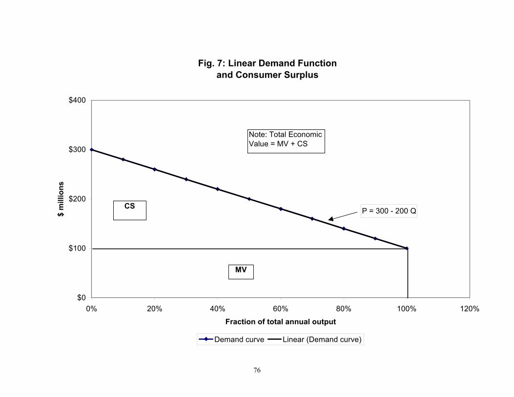
76

Fig. 7: Linear Demand Functionand Consumer Surplus

P = 300 - 200 Q

$0

$100

$200

$300

$400

0% 20% 40% 60% 80% 100% 120%

Fraction of total annual output

$ m

illio

ns

Demand curve Linear (Demand curve)

CS

MV

Note: Total Economic Value = MV + CS

77

7. Now dP/dQ is the slope of the demand function, and for a linear function the slope isconstant over any portion of the curve or indeed for the curve as a whole.

8. Therefore, dP/dQ = ∆P / ∆Q = (MP – P0) / (Q1 – Q0).

9. Substituting for MP, Q1, and Q0 in Eq. 8, we get dP/dQ = (MV-P0) / (1 - 0) = MV - P0.

10. Plugging Eq. 9 back into Eq. 6, we get MV = E1 * (MV-P0).

11. Solving Eq. 10 for P0, we obtain P0 = MV * [ (E1 – 1) / E1]

We can now derive a linear equation for Total Economic Value TEV as follows:

12. TEV equals the rectangular area MV plus the right triangular area CS (see Fig. 2, Sec. II).

13. Area of the rectangle = height x width; area of the right triangle = ½ x height x width.

14. Substituting these formulas in Eq. 12, we obtain TEV = (MP*Q1) + (P0–MV)*(Q1-Q0) / 2.

15. Plugging Eq. 11 into Eq. 14 and simplifying, TEV=MV+{MV*[(E1–1)/E1]–MV}/2.

16. Eq. 15 then simplifies to TEV = MV * ( 1 – 1 / 2E )

In addition to mathematical simplicity,63 the approach described above has the advantage ofproviding estimated values for TEV that are more conservative (i.e., lower) than those providedby non-linear demand functions. Fig. 8 (next page) compares the demand functions in Fig. 6 andFig. 7; to fit both demand curves on the same page, a logarithmic scale had to be used for thevertical axis.

What Figs. 6 and 8 clearly show is that TEV for a non-linear demand function increaseswithout limit; at Q = 10%, P has already reached $10 billion, compared with a value at Q =100% of only $100 million. Except possibly under extreme circumstances, it is unlikely that TEVwould reach such high levels when Market Value equals only $100 million. The linear demandfunction is clearly the more conservative of the two by a wide margin.

For any natural good for which we have an elasticity value, we can compute the ratio ofTEV or CS to MV using Equation 16 above. Table 36 below shows the calculations for eighttypes of natural goods covered in this study. As Table 36 shows, the excess of TEV over MVgrows in a non-linear fashion as elasticity increases towards zero, i.e., as demand becomes lesselastic (more inelastic). An increasingly inelastic demand is exactly what we would expect as thenatural good becomes more of a necessity (more essential) than a luxury good. Figure 9(following Table 36) shows this relationship graphically.

(text continues following figures and table)

63 While the derivations presented above may appear complex, those involving non-linear functions tendto be even more complex and require calculus techniques for their solution.

78

Fig. 8: Linear vs. Non-Linear Demand Curves (log scale)

$1

$10

$100

$1,000

$10,000

$100,000

0% 10% 20% 30% 40% 50% 60% 70% 80% 90% 100% 110%

Pct. of total annual volume

$ m

illio

ns (l

ogar

ithm

ic s

cale

)

Linear function Non-linear function

?

P = 100 / Q2

P = 300 - 200 Q

79

Table 36: Elasticity, Consumer Surplus, and Economic ValueType of Natural Good Elasticity* TEV / TMV CS / TMVFarm products-weighted avg (1) -0.069 8.21 721%Game animals -0.089 6.62 562%Fish (finfish and shellfish) -0.098 6.10 510%Timber-median (2) -0.250 3.00 200%Fuelwood -0.340 2.47 147%Water-midpoint (3) -0.400 2.25 125%Minerals-midpoint (4) -0.600 1.83 83%Fur-bearing animals -0.691 1.72 72%

*own-price short-run elasticity of demand.

TEV = Total Economic Value = TMV + CSTMV = Total Market Value = TEV - CSCS = Consumer Surplus = TEV – MV

1. Farm products-crops (87.68%) -0.067 8.46 746%Farm products-animals (12.32%) -0.092 6.43 543%

2. Timber-1st quartile -0.520 1.96 96%Timber-median -0.250 3.00 200%Timber-3rd quartile -0.100 6.00 500%

3. Water-low end -0.600 1.83 83%Water-middle -0.400 2.25 125%Water-high end -0.200 3.50 250%

4. Minerals-low end -1.000 1.50 50%Minerals-middle -0.600 1.83 83%Minerals-low end -0.200 3.50 250%

Sources of elasticity estimates:Farm products See Exhibit BGame animals USDA/Economics Research Service (meat)Fish USDA/Economics Research Service (fish)Timber Daigneault (2006)Fuelwood Skog (1993)Water Young (2005)Mineral aggregates Morrell (2006); USEPA (1997)Fur products USDA/ERS (clothing)

80

Fig. 9: Elasticity, Consumer Surplus, and Economic Value

0.0

1.0

2.0

3.0

4.0

5.0

6.0

7.0

8.0

9.0

0.00 0.10 0.20 0.30 0.40 0.50 0.60 0.70 0.80

Absolute value of elasticity of demand

Rat

io to

Mar

ket V

alue

0%

100%

200%

300%

400%

500%

600%

700%

800%

900%

Pct.

of M

arke

t Val

ue

Total Economic Value / Market Value Consumer Surplus / Market Value

TEV / MV

CS / MV

81

It should be noted that the market values and the elasticity estimates used in this study comefrom different sources, and there is a difficult-to-quantify risk that elasticities estimated usingnon-New Jersey data might differ from elasticities based on New Jersey-specific data. Forexample, Equation 4 above assumes that our point estimates of elasticity E1 apply at the Q1 endsof the related demand curves, i.e., the ends where demand is greatest. However, Nicholson(2002) points out that a common practice in empirical work is to report estimated elasticitiesbased on the average price for the good in question. This could mean that the elasticity estimateson which this study relies apply somewhere in the middle of the various demand curves ratherthan at their maximum-demand ends.

Even if it applies, however, this possibility may not pose a significant problem for ourpurposes. Suppose, for example, that an empirical study derived an elasticity of –0.5 based on a“price point” halfway between Q0 and Q1. It can easily be shown that for a linear demand curve,elasticities are lower at the Q1 end (where the marginal percentage changes in Q are smaller andthose in P larger) and higher at the Q0 end (where the marginal percentage changes in Q arelarger and those in P smaller). Therefore, the elasticities above (to the right of) the halfway pointin this case should be smaller than –0.5. However, as Fig. 9 shows, the lower the elasticity, thegreater the add-on for CS and therefore the higher the TEV. The assumption in Equation 4 thatthe –0.5 elasticity applies at the Q1 end of the curve is therefore conservative, i.e., it results inlower estimates for CS and TEV.

If the elasticities of any of our natural goods were close to zero, we would face the problemof demand functions whose values increase exponentially without limit and become undefinedwhen quantity equals zero. For example, if E = -0.001, the ratio of TEV to MV becomes 501,and the CS add-on becomes 50,000% of MV. There are only two natural goods “produced” inNew Jersey whose elasticities might be that low, namely air and water. The above method mightindeed not work well for air, and this study does not attempt to estimate a value for that “good”.

As to water, most empirical studies have found elasticities ranging from –0.2 to –0.6 ratherthan closer to zero (Young 2005). While these findings may seem surprising for such a clearlyessential good, they reflect in part the existence of multiple uses for. While the elasticity ofdemand for drinking water may in fact be close to zero, most uses of water are not as essential,and some, such as watering lawns and other green spaces, are much less essential and thereforemuch more likely to be influences by price changes.64 The empirically-determined elasticityrange for water may indicate that a substantial part of our use of water is in fact non-essential.

In conclusion, the approach developed in this appendix allows us to calculate reasonable andconservative first-order linear estimates of the Total Economic Values of the provisioningservices delivered by New Jersey’s natural capital. Sections III-IX of the main report apply theapproach to specific types of natural goods.

64 This suggests that the demand for water is not completely linear, since linear demand implies theexistence of a price above which no water is demanded. As noted above, the assumption of linearity is afirst-order approximation of the “true” demand curve.

82

Appendix B: Elasticity in Linear Demand Functions

As noted in Appendix A, while a linear demand function is easy to manipulatemathematically, elasticity is not constant along the demand curve, as shown in the followingexample based on the linear demand function shown in Fig. 7. The example uses the concept of“arc” elasticity, in which the midpoints of the Q and P intervals are used to calculate thepercentage changes in Q and P respectively.

• If demand drops from 100 units to 90 units, the change is -10 units; the midpoint of thearc is (100+90)/2 = 95, and the percentage change in demand is –10/95 = -10.5%. If theprice related to the demand change increases from $100 to $120, the change is +$20; thearc midpoint is (100+120)/2 = $110, and the percentage change in price is +20/110 =+18.2%. The elasticity of demand over this range is therefore –10.5% / +18.2% = -0.58.

• If demand drops again from 90 units to 80 units, the change equals -10 units; themidpoint is (90+80)/2 = 85, and the percentage change in demand is –10/85 = –11.8%.If the unit price increases from $120 to $140, the change is +$20; the midpoint of thearc is (120+140)/2 = $130, and the percentage change in price is +20/130 = +15.4%.The price elasticity of demand over this range is therefore –11.8% / +15.4% = -0.77.

In each case, price increases by $20 and quantity demanded decreases by 10 units; however, thesignificance of those changes in percentage terms depends on the absolute levels from which thepercentage changes are measured. Constant elasticity means that the marginal elasticity isconstant everywhere on the demand curve.

Although the linear demand function shown in Fig. 7 does not exhibit such constantelasticity, it does have the property that over larger intervals, “overall elasticity” is constant aslong as the percentage changes in P and Q are measured from MP and Q1 respectively. Forexample, for the same linear demand function:

• If demand drops from 100 units to 90 units, the percentage change in demand is –10/100 = -10%. If the related price change is from $100 to $120, the percentage pricechange is +$20/$100 = +20%. Overall elasticity for this range is –10%/+20% = -0.5.

• Similarly, if demand drops to 80 units, the percentage change in demand measured fromQ1 is –20/100 = -20%. If the related price increases to $140, the percentage pricechange measured from P1 is +$40/$100 = +40%. Overall elasticity for this range equals–20%/+40% = -0.5.

It is easy to show that for the demand function in Fig. 7, overall elasticity remains at –0.5 for anyvalue of Q between 1.0 and 0.0 as long as the percentage changes in P and Q are measured fromMP and Q1 respectively. While overall elasticity is not a recognized concept in standardeconomics, it does show that a weaker type of constancy exists for linear demand “elasticity”.

83

Appendix C: Alternate Farmland Valuations

The estimates of farmland value presented in Section V are based on the land’s continueduse for farming and on net farm income as the metric for the annual flow of value fromfarming.65 In the New Jersey real estate market, however, there are probably few sales offarmland in which a substantial portion of the sale price is not due to the land’s potential as a sitefor commercial or residential development. That is, the market value of farmland reflects bothits continued use to produce agricultural products and its development potential.

In that regard, NASS and ERS have reported different estimates for the market value of NewJersey farmland as Table 37 shows (COA = Census of Agriculture; NFI = net farm income).

Table 37: Estimated Market Value of New Jersey Farmland ($/acre)Source Coverage 2002 2004 CalculationNASS Census of Agric. Land + all bldgs. 9,137 n/a Note ANASS Census of Agric. Land + all bldgs. 9,245 n/a Note BNASS Land Values All farmland 8,600 9,750 Note CNASS Land Values Cropland 9,000 9,900 Note CNASS Land Values Pastureland 9,700 10,600 Note CNASS Land Values All farmland 9,224 10,124 Note DERS Balance Sheet Land + farm bldgs. 7,615 8,487 Note E

A. As reported by NASS in the 2002 Census of Agriculture (COA); includes dwellings.

B. Market value/farm (including dwellings) / acres/farm from 2002 COA.

C. As reported by NASS in Land Values and Cash Rents 2004 Summary, August 2004.

D. NASS 2002 or 2004 cropland and pastureland values/acre x 2002 COA cropland andpastureland shares of total acreage.

E. ERS 2002 or 2003 balance sheet figure for real estate assets (excluding dwellings) / totalfarm acreage from 2002 COA or 2003 acreage estimate; 2003 price/acre is inflated to2004.

The large differences between the ERS and NASS estimates may be due to the fact that NASSincludes the value of farm dwellings in its farm balance sheet estimates; since dwellingsconstitute physical or “built” capital, ERS’s figures might seem to come closer to the “pure”natural capital value we are seeking.

As stated in Section V, a 2002 study by Plantinga et al. using 1997 data concluded that 82%of the value of New Jersey farmland could be attributed to development potential. Based on thatfigure, we might multiply the 2004 ERS land value estimate of $8,487/acre by 18% to obtain$1,528/acre as an estimate for the market value of New Jersey farmland as farmland, i.e., net of

65 Some portion of net farm income could be attributed to the cost of the owner’s or operator’s human andfinancial capital and another portion to a premium for risk-taking (Pearce 1992), i.e., to bearing the risk ofloss inherent in agriculture (other than risks covered by crop insurance or similar safeguards).

84

both dwellings and development potential.66 This figure is much lower than the average presentvalue of $9,570 presented in Section V, a figure that is based solely on the value of farm outputin perpetuity.

The estimated land value from farming of $1,528/acre is potentially compatible with theactual average cash flow from farming (net cash farm income) of $222/acre/year calculated inSection V. In principle, the value of land attributable to farming should equal the present value ofthe annual cash flows from farming. That present value depends on two factors—the discountrate and the time horizon; since we are now examining actual price data (or estimates thereof),discounting by 3%/yr in perpetuity is not the only possibility.

We can shed some light on this by using a plausible range of time horizons and discountrates to calculate the present value of the annual cash flow of $233/ac/yr (see Table 14, SectionV), which in principle should equal the value of the land from farming. The results for selecteddiscount rates are as follows (NCFI = net cash farm income):

Table 38: Net Farm Income and Agricultural Value of FarmlandYears NCFI/ac/yr PV rate PV of NCFI Assumed price

10 $233 8.50% $1,529 $1,52811 233 9.80% 1,527 1,52812 233 10.80% 1,527 1,52813 233 11.60% 1,526 1,52814 233 12.20% 1,529 1,52815 233 12.70% 1,529 1,52816 233 13.15% 1,526 1,52817 233 13.45% 1,530 1,52818 233 13.75% 1,528 1,52819 233 14.00% 1,526 1,52820 233 14.15% 1,530 1,528

The values in this table represent the type of analysis that owners of farmland might engagein to estimate the present value of their land based solely on the annual flow of net income fromfarming, the owners’ time horizons, and their projected or desired rates of return. In effect,landowners with different time horizons could in principle arrive at the same estimated value of$1,528/acre from farming if they also had different rates of return in mind.

For periods shorter than about ten years, the discount rates needed to equate the presentvalue of the annual cash flow from farming to the estimated market price of $1,528/acre becomeimplausibly low, meaning that owners of farmland would probably demand higher rates of returnfrom their investment in agriculture. Similarly, as the time horizon increases, the discount ratesneeded to equate the present value of the annual cash flow from farming to the estimated market

66 The resulting estimate would still include non-residential farm structures such as barns, silos, etc. andwould therefore still somewhat overestimate the value of the land itself. Presumably such structures onlyhave value if the land continues to be farmed.

85

price of $1,528/acre may become implausibly high, meaning that they may exceed the rates ofreturn that such landowners could expect to realize.

This analysis suggests that USDA’s estimated values for New Jersey farmland—which relyon self-reported estimates provided by farmers themselves and by other sources—are based onthe assumption of a fairly short time horizon for the continuation of agricultural activities. This isprobably not unreasonable in the New Jersey context, especially given that the average age offarmers was 55 according to the 2002 Census of Agriculture. 67

The cash flow and land price methods as presented in this study can thus be made consistentif we assume that the landowner’s valuation of agricultural income is based on a relatively shorttime horizon. However, since the focus of this study is on the value of goods provided by NewJersey’s natural capital, the estimated per-acre value presented in Section V is based solely oncontinued use of farmland as farmland rather than on future development potential and the saleof development options.

67 A possible implication of this assumption is that the option to sell farmland for development is valuedas though it would not be exercised until the current farm owner or operator retires, which again may be areasonable assumption in the New Jersey context.

86

Appendix D: Valuation of Standing Sawtimber

Forest economics recognizes two theoretical methods for valuing standing timber onforested land, both involving present value techniques. The first values the standing timber at amoment in time, assuming that no regeneration will take place as trees mature and die or are cut(harvested); in effect, harvesting of timber is assumed to be restricted to the current rotationcycle. The unit values are based on biomass growth (wood volume) as modified by economicfactors such as timber price. In this case, the value of standing timber equals the timber volume(at a specific point in time) multiplied by the stumpage price multiplied by the discount factor.

The second theoretical valuation method assumes that harvesting can be sustainedindefinitely, so that the value of the forest asset can be calculated as the present value of anindefinite annual stream of rent generated from harvesting the timber stock. In effect, thisapproach values the forest “estate” composed of timber and land combined. In this method, thevalue of standing timber is equal to the discounted future stumpage price for mature timber afterdeducting the costs of bringing the timber to maturity. The stumpage price is the price paid bythe logger to the owner of the forest for the right to log standing timber. The costs includethinning (net of any receipts), other forest management costs and rent on the forestland. Fornatural (or non-cultivated) forests the management costs are very low or minimal. For this case,the value of standing timber equals the discounted future stumpage price minus the costs.

Applying either of the two present value methods to actual forests is relatively complicatedand requires a great deal of data on the age structure and growth rate of the forest, forestmanagement costs, and the rent on forest land. As a result, various simplified methods have beendeveloped and are applied. Two such valuation approaches are the stumpage valuation andconsumption value methods.

The stumpage valuation method, also known as the net price method, assumes that thediscount rate is equal to the forest’s natural growth rate. Since the two rates then cancel eachother out, this assumption eliminates the need for discounting, so the value of the stock can beobtained simply by multiplying the current volumes of standing timber by the stumpage prices(neglecting costs).68 In many applications, the value of the standing timber is based on thereceipts from harvesting mature timber only, while costs are neglected. The assumption is thatreceipts are only realized when the timber reaches maturity. Maturity depends on physicalgrowth but also involves economic factors in its definition. The stumpage prices are reflected inthe receipts and therefore directly obtainable. The average stumpage price is calculated dividingthe stumpage value by the volume of the removals.

An advantage of the stumpage value method is that it can be used to value all the itemsrelated to physical timber accounting in a simple way, including stocks, removals, naturalgrowth, and other changes. This is not the case for other valuation methods. In the stumpagevaluation method an average stumpage price is obtained and applied to the whole stock ofstanding timber. In its simplest formulation, no discrimination is made for the age of the timber 68 This approach is somewhat similar to the Hotelling method except that the discounting is offset byphysical growth rather than by price increases. For a further discussion, see Hotelling, J. (1931). “TheEconomics of Exhaustible Resources,” Journal of Political Economy, 39, pp. 137 – 175.

87

at the valuation date. Other methods require data for different age or diameter classes, whichcomplicate the calculation of the value of the timber stocks, and consequently, of other items inthe physical timber accounts since the valuation of these items should be consistent with thatused for stocks.

The consumption value method uses different stumpage prices not only for different treespecies but also for different age or diameter classes. These prices are applied to the stock oftimber based on information on species mix and age or diameter classes obtained from forestinventories. The consumption value method measures the value of the timber as if it were all cutnow, hence its name. Which of the methods gives reasonably accurate results depends on thecharacteristics of the forest stock to be valued and the current and expected exploitationconditions and harvesting patterns. The stumpage valuation method gives good results when thecurrent stock and harvesting structure can be assumed to continue in the future. The consumptionvalue method yields good results for old growth forests, a category which generally does notinclude New Jersey’s forests.

88

List of Exhibits

Exhibit A: Water Losses for Major Regulated Water Utilities in New Jersey

Exhibit B: Market Value and Elasticity of Demand for New Jersey Agricultural Products

Exhibit C: Econometric Estimates of Timber Demand Elasticity

89

Exhibit A: Water Losses for Major Regulated Water Utilities in New Jersey

Utility Loss Pct. 000 Gal. Lost 000 Gal. Demand # CustomersElizabethtown Water 16.80% 9,057,621 53,914,411 206,583Gordon's Corner 7.98% 163,715 2,051,566 14,526Middlesex Water 11.09% 1,933,924 17,438,449 58,354Mount Holly Water 21.70% 399,977 1,843,212 16,064New Jersey American 23.10% 9,721,539 42,084,584 361,502Shorelands Water 3.44% 64,782 1,883,198 11,091United Water NJ 23.10% 9,721,539 42,084,584 193,379United Water Toms River 12.97% 599,888 4,625,197 48,557Subtotal 19.08% 31,662,985 165,925,201 910,056Avg. gal./customer (000) 182Aqua NJ: Northern division 23.43% 318,759 1,360,474 38,097 Central division* 10.10% 386,355 3,825,293 Southern division 3.37% 59,320 1,760,237Subtotal 11.01% 764,434 6,946,004 38,097Avg. gal./customer (000) 182

Total or average 18.76% 32,427,419 172,871,205 948,153NJ total per 1996 NJSWSP (based on 1,499.1 MGD) 547,171,500Share of above in NJ total 31.6%

Weighted avg. Excluded shareNJ avg. if excluded sources = 10.0% 12.8% 68.4%NJ avg. if excluded sources = 20.0% 19.6% 68.4%NJ avg. if excluded sources = 30.0% 26.4% 68.4%Major utilities not included (no data):Trenton Water 61,873Village of Ridgewood 19,857Wildwood Water Utility 13,197Total customers of regulated utilities 1,118,500* demand inferred from no. of customers and avg. demand per customer for other major utilities; loss pct.obtained by NJBPU staff from utility annual report.Note: regulated utilities are those for which NJBPU sets rates; major utilities are those with 10,000 ormore customers as of 7/1/05. Figures do not include unregulated water purveyors, self-supplied demand(e.g., private wells), etc. Loss percentages may not apply to excluded sources.Sources: information obtained by NJBPU staff from utility annual reports and rate orders and calculationsby NJDEP. N/a = not available.

90

Exhibit B: Market Value and Elasticity of Demandfor New Jersey Agricultural Products

Type of Agricultural Product 2002 $000 Elasticity WeightsNursery, greenhouse, floriculture, sod $ 356,863 n/a n/aVegetables, melons, potatoes 167,956 -0.070 -11,757Fruits, tree nuts, and berries 87,148 -0.070 -6,100Oilseed, dry beans, dry peas 20,352 -0.047 -957Hay, holiday trees, SRWC*, other 15,643 n/a n/aGrains 9,533 -0.040 -381

Total crops (87.68%) 657,494 -0.067 -19,195

Milk / other dairy products from cows $ 29,154 -0.095 -2,770Poultry & eggs 26,041 -0.092 -2,396Other livestock & animal products** 18,870 -0.089 -1,679Horses/ponies/mules/burros/donkeys 18,314 n/a n/a

Total animal products (12.32%) 92,378 -0.092 -6,845

Total current production for sale*** $ 749,872 -0.069 -26,040

* SRWC = short-rotation woody crops. N/a = not available.

** includes cattle & calves; hogs & pigs; sheep, goats, & their products; aquaculture; and otheranimals and animal products.

*** excludes machine hire & customwork, forest products sold, other farm income, & grossimputed rental value of farm dwellings.

NASS 2002 = US Department of Agriculture, National Agricultural Statistics Service, 2002Census of Agriculture.

Elasticities from USDA, Economics Research Service. Weights = market value x elasticity.

n/a = not available

91

Exhibit C: Econometric Estimates of Timber Demand Elasticity

Study Region Product Elasticity*Adams et al. (2002) Western OR Sawlogs -2.00Polyakov et al. (2004) Alabama Pulpwood -1.72Adams et al. (2002) Western OR Private timber -1.58Merrifield and Haynes (1985) Pacific NW Plywood -0.85Connaughton et al. (1988) Montana Stumpage -0.65Newman (1987) South Sawtimber -0.57Robinson (1974) South Softwood -0.52Abt et al. (2000) Southeast Timber products -0.50Newman (1987) South Pulpwood -0.43Carter (1992) Texas Pulpwood -0.41Adams et al. (2002) Western OR Timber for plywood -0.36Adams et al. (2002) Western OR Timber for lumber -0.26Abt (1987) South Lumber -0.25

Median -0.25Robinson and Fey (1990) South Softwood -0.25Abt (1987) West Lumber -0.20Haynes et al (1981) Pacific NW Softwood -0.17Haynes et al (1981) Pacific NW Softwood -0.14Haynes et al (1981) South Central Softwood -0.13Merrifield and Singleton (1986) Pacific NW Plywood -0.10Abt and Kelly (1991) FL and GA Softwood -0.10Connaughton et al. (1988) Montana Stumpage -0.09Merrifield and Haynes (1985) Pacific NW Lumber -0.07Haynes et al (1981) Southeast Softwood -0.05Daniels and Hyde (1986) N. Carolina Hard and Soft -0.03Merrifield and Singleton (1986) Pacific NW Lumber -0.01Merrifield and Haynes (1985) Pacific NW Lumber -0.001

*Short-run own-price elasticity of demand

Sources: compiled by A. Daigneault, USEPA, and W. Mates, NJDEP

92

REFERENCES

General

Bockstael, N. and K. McConnell, Calculating Equivalent and Compensating Variation forNatural Resource Facilities. Land Economics, vol. 56, no. 1, February 1980.

Costanza, R. et al. 2006. The Value of New Jersey’s Ecosystem Services and Natural Capital.Burlington, VT: University of Vermont (release pending).

Hasse, J. and R. Lathrop. 2001. Measuring Urban Growth in New Jersey. Rutgers University.Available at http://users.rowan.edu/~hasse/nj_urbangrowth/nj_urban_growth.pdf.

MECA 2001. Climate Change and a Global City: An Assessment of the Metropolitan East CoastRegion. Report prepared by the Columbia Earth Institute for the U.S. Global Climate ChangeResearch Program. July 2001. Available at http://www.usgcrp.gov/usgcrp/nacc/metro.htm.

MEA 2003. United Nations Environment Programme (UNEP). Millennium EcosystemAssessment. Ecosystems and Human Well-being: A Framework for Assessment. Available athttp://www.maweb.org/en/index.aspx.

National Research Council 1995. Beach Nourishment and Replenishment, Appendix E:Economic Concepts and Issues. Washington: National Academy Press.

New Jersey Department of Environmental Protection. Bureau of Geographic InformationServices. 1986 and 1995/97 Land use/Land cover data by Anderson LULC code.

Nicholson, Water 2002. Microeconomic Theory: Basic Principles and Extensions, 8th ed. South-Western/Thomson Learning, Inc.

Pearce, D. W., ed. 1992. The MIT Dictionary of Modern Economics, 4th ed. Cambridge, MA:The MIT Press.

Tietenberg, Tom 2000. Environmental and Natural Resource Economics, 5th ed. Addison WesleyLongman, Inc.

U.S. Department of Labor, Bureau of Labor Statistics. U.S. All Items Urban Consumer PriceIndex. Available at http://www.bls.gov/cpi/home.htm#data.

Washington State University 2005. Revised Small Business Economic Impact Statement,Instream Resources Protection and Water Resources Program, Stillaguamish River Basin,Chapter 173-505 WAC. Reference # 05-11-030, August 2005.

DiscountingDaly, H. and J. Cobb, Jr.. 1999. For the Common Good: Redirecting the Economy TowardsCommunity, the Environment, and a Sustainable Future. Beacon Press, Boston 1999.

Newell, R. and W. Pizer. 2001. Discounting the benefits of climate change mitigation: Howmuch do uncertain rates increase valuations? Prepared for the Pew Center on Global ClimateChange, December 2001.

Newell, R. and W. Pizer. 2003. Discounting the distant future: how much do uncertain ratesincrease valuations? Journal of Environmental Economics and Management 46, 52-71.

93

U.S. Office of Management and Budget. Circular A-4, “Regulatory Analysis”, September 17,2003. Available at http://www.whitehouse.gov/omb/circulars/a004/a-4.pdf.

Weitzman, M. 2001. Gamma Discounting. Amer. Econ. Rev., vol. 91, no. 1, March 2001.

Water SupplyNew Jersey Department of Environmental Protection. New Jersey Statewide Water Supply Plan.Trenton, New Jersey, August 1996.

New Jersey Geological Survey. Digital Geodata Series, DGS04-9, New Jersey waterwithdrawals, transfers, and discharges by Watershed Management Area, 1990-1999. Availableat http://www.state.nj.us/dep/njgs/geodata/dgs04-9.htm.

New Jersey State Climatologist. Monthly Precipitation in New Jersey from 1895-2006.Available at http://climate.rutgers.edu/stateclim_v1/data/njhistprecip.html.

Watson, K. et al. 2005. Streamflow Characteristics and Trends in New Jersey, Water Years1897-2003. U.S. Geological Survey Scientific Investigations Report 2005-5105. Available athttp://pubs.usgs.gov/sir/2005/5105/.

Water RatesNew Jersey Board of Public Utilities. BPU Docket No. WO02040238A, 12/18/02. Order IMONew Jersey American Water Company. Available at http://www.state.nj.us/bpu/wwwroot/water/WO02040238AORD.pdf.

New Jersey Board of Public Utilities. BPU Docket No. WR03070511, 2/18/04. Order IMONew Jersey American Water Company. Direct Testimony and Exhibits of Brian Kalcic onbehalf of the New Jersey Division of the Ratepayer Advocate. Available athttp://www.state.nj.us/rpa/Kalcic_njaw.pdf.

New Jersey Board of Public Utilities. BPU Docket No. WR03090714, 5/24/04. Order IMOGordon’s Corner Water Company. Available at http://www.state.nj.us/bpu/wwwroot/water/WR03090714_20040527.pdf.

New Jersey Board of Public Utilities, Division of Water, Bureau of Rates. Residential Rates andAverage Water Bill Analysis, Rates in Effect July 1, 2005. Separate analyses for metered andunmetered service provided by agency staff.

Water ValuationAsian Development Bank, 1996. Water Management and Allocation Options: Angat RiverSystem. Final Report to the National Water Resources Board, Republic of the Philippines. R.A.Young et al., Annex 5: Economic and Institutional Considerations. ADB Technical assistancereport TA No. 2417-PHI.

Gibbons, D. C. 1986. The Economic Value of Water. Washington: Resources for the Future.

James, L. D. and R. R. Lee, 1971. Economics of Water Resource Planning. New York:McGraw-Hill.

Saleth, R.M. and A. Dinar 1997. Satisfying Urban Thirst: Water Supply Augmentation andPricing Policy in Hyderabad City, India. World Bank Technical Paper No. 395, November 1997.

94

U.S. Environmental Protection Agency. A Framework for Measuring the Economic Benefits ofGround Water. EPA 230-B-95-003, pub. October 1995.

U.S. Environmental Protection Agency. Community Water System Survey 2000, Volume II.EPA Report EPA 815-R-02-005B. Pub. December 2002. Available at http://www.epa.gov/safewater/consumer/pdf/cwss_2000_volume_ii.pdf.

Young, R.A. 1998. Water Management Options for Ceara and Piaui, Brazil. Consulting reportdated October 20, 1998.

Young, R. 2005. Determining the Economic Value of Water: Concepts and Methods. Resourcesfor the Future, Washington DC.

Young, R.A. et al. 1972. Economic Value of Water: Concepts and Empirical Estimates. FinalReport to the National Water Commission. NTIS document PB-210-356.

Mineral ResourcesMorrell, S. O. 2006. The Initial Price Impact of Closing the Production of Crushed Rock in theLake Belt Region of Miami-Dade County. Florida Tax Watch, Research Report, June 2006.Available at http://www.floridataxwatch.org/resources/pdf/LakeBeltMiningImpact.pdf. Accessedoctober 23, 2006.

Moulin, R. 1996. Economics of the Aggregate Market. Available at http://www/em.gov.bc.ca/geolsurv/Surficial/forum/fpaper3.htm. Accessed 10/24/06.

National Mining Association, various years. Mining in New Jersey. Available at www.nma.org.

U.S. Environmental Protection Agency 1997. Regulatory Impact Analyses for the ParticulateMatter and Ozone National Ambient Air Quality Standards and Proposed Regional Haze Rule.Appendix H: Economic Impacts Supporting Information. July 17, 1997. Available athttp://www.epa.gov/ttn/oarpg/naaqsfin/ria.html. Accessed October 2006.

U.S. Geological Survey 2004. Minerals Yearbook: The Mineral Industry of New Jersey.Available at http://minerals.usgs.gov/minerals/pubs/state/nj.html.

U.S. Geological Survey 2006. Mineral Commodity Summaries. Available at http://minerals.usgs.gov/minerals/pubs/mcs/. Accessed October 23, 2006.

U.S. Geological Survey, various years. Minerals Yearbook. Available athttp://minerals.usgs.gov/. Entries for construction sand and gravel, silica (includes industrial sandand gravel), and crushed stone.

Agricultural ProductsPlantinga, A.J. et al. 2002. The effects of potential land development on agricultural land prices.Journal of Urban Economics 52:561-581 (2002).

U.S. Census Bureau, County Business Patterns, various years. Available at http://censtats.gov.Accessed 3/7/06.

U.S. Census Bureau, Nonemployer Statistics, various years. Available athttp://www.census.gov/epcd/nonemployer. Accessed 3/7/06.

95

U.S. Department of Agriculture, Economic Research Service. Price Elasticity for FoodSubgroup. Available at http://www.ers.usda.gov/Data/InternationalFoodDemand. Accessed9/22/06.

U.S. Department of Agriculture, Economic Research Service. Value added to the U.S. economyby the agricultural sector via the production of goods and services, 2000-2004, and Farmbusiness balance sheet, New Jersey, 2000-2003. Provided by Roger Strickland,rogers@ers.usda.gov; also available through http://www.ers.usda.gov.

U.S. Department of Agriculture, Economic Research Service. State Fact Sheets: New Jersey.Available at http://www.ers.usda.gov/StateFacts/NJ.htm. Accessed 8/28/06.

U.S. Department of Agriculture, National Agricultural Statistics Service. 2002 Census ofAgriculture-State Data-New Jersey. Available at http://www.nass.usda.gov/census/census02/volume1/nj/index1.htm.

U.S. Department of Agriculture, Economic Research Service. Retail-Farm Price Margins andConsumer Product Diversity. Technical Bulletin No. 1899, April 2002. Available atwww.ers.usda.gov/publications/tb1899.

U.S. Department of Agriculture, National Agricultural Statistics Service. Land Values and CashRents, 2004 Summary. August 2004. Available at http://usda.mannlib.cornell.edu/reports/nassr/other/plr-bb/land0804.pdf.

U.S. Department of Agriculture, National Agricultural Statistics Service. New Jersey StateAgriculture Overview-2004.

U.S. Department of Commerce, Bureau of Economic Analysis. Gross Domestic Product byIndustry Accounts. Available at http://www.bea.gov/industry. Various tables; accessed 8/10/06.

U.S. Department of Commerce, Bureau of Economic Analysis. Gross State Product Data Tablesfor New Jersey. Available at http://www.bea.gov/regional. Various tables; accessed 9/28/06.

Non-Farm AnimalsDivision of Fish and Wildlife, New Jersey Department of Environmental Protection. Websitehttp://www.state.nj.us/dep/fgw. Various web pages accessed 8/15-16/06, including Hunting inNew Jersey, Deer Harvest Data, Biology of the White-Tailed Deer, Black Bear Hunting SeasonResults for 2003 and 2005, Estimated Game Bird Harvest 1985-2003, Estimated Small GameFirearm Harvest 1985-2004, Estimated Fur-Trapping Harvest 1981-2004, and New JerseyTrapper Harvest, Recreational and Economic Surveys for 2003-04 and 2004-05.

Division of Fish, Game and Wildlife 1999. Governor’s Report on Deer Management in NewJersey. Trenton: New Jersey Department of Environmental Protection, October 1999.

U.S. Fish and Wildlife Service. 2001 National Survey of Fishing, Hunting, and Wildlife-Associated Recreation. Pub. 2003 by the U.S. Department of the Interior, US Fish and WildlifeService, and other agencies. New Jersey data available at http://www.census.gov/prod/2003pubs/01fhw/fhw01-nj.pdf.

U.S. Department of Agriculture, Economic Research Service. Price Elasticity for BroadConsumption Groups. Available at http://www.ers.usda.gov/Data/InternationalFoodDemand.Accessed 9/28/06.

96

U.S. Department of Labor, Bureau of Labor Statistics. Northeast Urban Consumer Price Index,selected meat items. Available at http://www.bls.gov/cpi/home.htm#data. Accessed 8/15/06.

Non-Farm PlantsNiles, L.J. et al. 2001. New Jersey’s Landscape Project: Wildlife Habitat Mapping forCommunity Land-Use Planning and Endangered Species Conservation. Project report issued bythe New Jersey Department of Environmnetal Protection, Division of Fish and Wildlife.

Simpson, R. D., Sedjo, R. A. and Reid, J. W. 1996. Valuing Biodiversity for Use inPharmaceutical Research. Journal of Political Economy 104: 163-185.

Fish and ShellfishNational Marine Fisheries Service. Commercial Fisheries Database http://www.st.nmfs.noaa.gov/st1/commercial/index.html (various pages; accessed various dates).

National Marine Fisheries Service. Recreational Fisheries Statistics http://www.st.nmfs.noaa.gov/pls/webpls/mr_catch_snapshot.results (accessed 8/15/06).

Responsive Management, 2003. New Jersey Anglers' Participation in Fishing, Harvest Success,and Opinions on Fishing Regulations. Survey conducted for the New Jersey Division of Fish andWildlife.

Southwick Associates, Inc. 2005. The Economics of Recreational and Striped Bass Fishing.Report prepared for Stripers Forever. Fernandina Beach, FL. Available atwww.stripersforever.org.

FuelwoodMurray, Brian T. 2004. “Homeowners Chop Heating Costs”. Article from the Newark Star-Ledger, 11/9/04. Available at http://sierraactivist.org/print.php?sid=45835. Downloaded 10/2/06.

Skog, K. E. 1993. Projected Wood Energy Impact on U.S. Forest Wood Products. Demandelasticities cited in Tables 1-2, p. 23. In: Proceedings of the 1st biomass conference of theAmericas: Energy, environmental, agriculture, and industry. National Renewable EnergyLaboratory, 1993:18-32, Vol. I.

U.S. Department of Agriculture, U.S. Forest Service. D. Griffith and R. Widman, ForestStatistics for New Jersey: 1987 and 1999. Resource Bulletin NE-152, pub. 2001. At http://www.fs.fed.us/ne/newtown_square/publications/resource_bulletins/pdfs/2001/ne_rb152p.pdf.

U.S. Energy Information Administration. Energy Consumption Estimates by Source, SelectedYears, 1960-2001. New Jersey data available at http://www.eia.doe.gov/emeu/states/sep_use/total/pdf/use_nj.pdf.

U.S. Energy Information Administration. Energy Price and Expenditure Estimates by Source,Selected Years 1970-2001. New Jersey data available at http://www.eia.doe.gov/emeu/states/sep_prices/total/pdf/pr_nj.pdf.

Timber SupplyDiGiovannia and C. Scott, Forest Statistics for New Jersey--1987. U.S. Department ofAgriculture, U.S. Forest Service. Resource Bulletin NE-112.

97

Griffith, D. and R. Widman, Forest Statistics for New Jersey: 1987 and 1999. U.S. Departmentof Agriculture, U.S. Forest Service. Resource Bulletin NE-152, pub. 2001. At http://www.fs.fed.us/ne/newtown_square/publications/resource_bulletins/pdfs/2001/ne_rb152p.pdf.

Northeastern Research Station, U.S. Department of Agriculture, U.S. Forest Service. Trends inNew Jersey Forests. Publication NE-INF-148-02 (informational brochure).

Widmann, R. 2004. Forests of the Garden State. U.S. Department of Agriculture, U.S. ForestService. Resource Bulletin NE-163.

Timber PricesAlabama Forestry Commission. Forest Resource Report 2004. Available athttp://www.forestry.state.al.us/publication/pdfs/Forest%20Resource%20Report%202004.pdf.

Illinois Department of Natural Resources and Illinois Agricultural Statistics Service. IllinoisTimber Prices. Available at http://ilvirtualforest.nres.uiuc.edu/harvest/t_prices.htm.

Maine Department of Conservation, Maine Forest Service. 2004 Stumpage Price Report.Available at http://mainegov-images.informe.org/doc/mfs/pubs/pdf/stumpage/04stump.pdf.

New York State Department of Environmental Conservation. Stumpage Price Reports, No. 64(Winter 2004) and No. 65 (Summer 2004). Available at http://www.dec.state.ny.us/website/dlf/privland/utilization/2004.pdf.

Pennsylvania State University, School of Forest Resources. Pennsylvania Woodlands Timbermarket Report. Available at http://www.sfr.cas.psu.edu/tmr/2004.HTM.

University of Maryland, College of Agriculture and Natural Resources. Maryland-DelawareStumpage Price Survey Results. Available at http://www.naturalresources.umd.edu/Stumpage_Prices.cfm.

University of Massachusetts, Department of Natural Resources Conservation. Southern NewEngland Stumpage Price Survey. Available at http://forest.fnr.umass.edu/snespsr/reports/new%2094%20on%20a.htm.

Timber Demand ElasticityAdams, D. et al. 2002. Timber Harvest Projections for Private Land in Western Oregon. OregonState University, College of Forestry.

Ando, A.W. 1997. The Price-Elasticity of Stumpage Sales from Federal Forests. Washington:Resources for the Future, Discussion Paper 98-06, November 1997.

Connaughton, K. et al. 1988. Alternative Supply Specifications and Estimates of RegionalSupply and Demand for Stumpage. U.S. Department of Agriculture, U.S. Forest Service. ForestService Research Paper PNW-RP-399, June 1988.

Daigneault, A. Summary of econometric studies of softwood stumpage demand and supplyelasticities. Personal e-mail communication, 10/2/06.

Prestemon, J. and R. Abt. Timber Products Supply and Demand, in Southern Forest ResourceAssessment Report. Available at www.srs.fs.fed.us/sustain.

Resources for the Future. The Economics of Global Timber Markets. September, 1997.

98

Schuler, A.T. 1978. An Econometric Analysis of the U.S. Hardboard Market. U.S. Departmentof Agriculture, U.S. Forest Service. Forest Service Research Paper NE-424.

Sendak, P. et al. 2003. Timber Supply Projections for Northern New England and New York.North. J. Appl. For. 20(4), 175-185.

Sohngen, B. et al. 1997. The Economics of Global Timber Markets. September 1997. Athttp://www.osti.gov/bridge/servlets/purl/755501-ymHeGQ/webviewable/755501.pdf.