Value Relevance of Income Tax Expense Post FIN 48

Leslie Robinson

Dartmouth College, Tuck School of Business leslie.a.robinson@tuck.dartmouth.edu

Pavel Savor Temple University, Fox School of Business

pavel.savor@temple.edu

Stephanie Sikes* University of Pennsylvania, Wharton School

ssikes@wharton.upenn.edu

April 9, 2017

ABSTRACT Using hand-collected data on the fraction of firms’ effective tax rates (ETRs) attributable to tax reserve changes, we examine how investors’ response to income tax expense changes after FIN 48 enactment. Consistent with investors viewing tax expense as value lost to taxes paid, in the pre-FIN 48 period we find that abnormal returns surrounding annual earnings announcements are negatively related to changes in firms’ ETRs and that abnormal returns surrounding 10-K filing dates are negatively related to the fraction of the ETR attributable to tax reserve changes. Following FIN 48 enactment, neither relation is statistically different from zero, suggesting that FIN 48 reduces the value relevance of income tax expense. However, the muted reaction is confined to firms for which we expect income tax expense to suffer the greatest decrease in value relevance, indicating that investors understand the differential impact of FIN 48 on tax reserve accruals.

JEL Classifications: H25, K34, M41 Keywords: FIN 48, accounting for income taxes, effective tax rate, valuation of tax expense We gratefully acknowledge financial support from The Wharton School’s Global Initiatives Research Program and research assistance by Tanya Paul and Xiaohan Ying.

*Corresponding Author

1

1. Introduction

Beginning in 2007, a new uniform set of rules governing accounting for uncertain tax

positions (ASC 740-10, Accounting for Uncertainty in Income Taxes, hereinafter “FIN 48”)

became effective. FIN 48 requires firms to evaluate each tax position using a two-step recognition

and measurement process, and to establish and disclose reserves for cash tax savings generated in

the current period that could be denied in the future if successfully challenged by a taxing authority.

Around the enactment of FIN 48, firms expressed concern that the new rules would force them to

accrue reserves for taxes that would never be paid. According to the Tax Executives Institute

(2011), anecdotal evidence supports the validity of these concerns. A potential consequence is that

income tax expense is now less informative about firms’ future tax payments. If investors do not

understand this, then firms could be mispriced as a result. However, the Financial Accounting

Foundation (FAF) (2012) concludes that FIN 48 disclosures allow financial statement users to

adjust income tax expense for estimates of the difference between preparers’ assessments under

FIN 48 and the possible results of the settlement process. This implies that investors can

appropriately anticipate reserve accruals that will likely be released in future periods without cash

consequences and that firms are not mispriced as a result of FIN 48. The objective of our study is

to evaluate which of the above two viewpoints is correct. Knowing the valuation implications of

FIN 48 is a crucial factor in assessing the real effects of the new rules. If firms are mispriced as a

result of FIN 48, it would be hard to argue that FIN 48 improved the financial reporting for income

taxes.

While there are numerous studies evaluating FIN 48, relatively few studies evaluate how

FIN 48 changed the financial reporting environment (Blouin and Robinson 2014). Until recently,

sufficient time had not passed for researchers to use the new disclosures to assess the longer-term

2

effects of this standard. Moreover, accounting for tax uncertainty was unobservable for most firms

prior to FIN 48 due to the lack of disclosure requirements.

In order to overcome this limitation and evaluate the earnings effect and associated

valuation consequences resulting from firms’ adoption of FIN 48, we hand-collect data on

increases and decreases to the effective tax rate (ETR) that are attributable to tax reserve changes

for each year beginning in 2004 and ending in 2012. We collect this data from firms’ rate

reconciliation tables as well as the text immediately surrounding the rate reconciliation table (e.g.,

explanations of “other” changes in the rate reconciliation). Our sample includes all firms in the

S&P 500 Index as of the end of 2004. To identify a FIN 48 effect, we denote fiscal years ending

December 31, 2004 through December 14, 2007 as the pre-FIN 48 period and all subsequent years

as the post-FIN 48 period.

We begin by examining the relation between changes in firms’ ETRs and abnormal returns

around the earnings announcement day (“announcement returns”). Consistent with investors

viewing tax expense as value lost to taxes paid (Thomas and Zhang 2014), we find that

announcement returns are significantly negatively related to changes in firms’ ETRs in the pre-

FIN 48 period. A one-standard-deviation increase in the change in a firm’s ETR decreases

announcement returns by 0.30 percentage points, which represents a meaningful economic effect.

However, in the post-FIN 48 period the relation is no longer statistically significant. These findings

hold in a variety of regression specifications and are consistent with changes in aggregate tax

expense being less value relevant in the post-FIN 48 period.

One explanation for the above finding is that FIN 48 results in changes in income tax

expense becoming less predictive of future tax-related cash outflows, and that investors consider

this when valuing firms. Changes in income tax expense could be less informative after FIN 48

3

because the recognition and measurement rules result in some firms booking greater reserves than

they need.1 However, we recognize that factors unrelated to FIN 48 could also affect firms’ ETRs

in the post-FIN 48 period (e.g., changes in valuation allowance accounts due to the financial crisis

and recession).

To more precisely identify whether the muted market reaction in the post-FIN 48 period is

attributable to investors deeming tax reserves as less value relevant, we examine the market

reaction to the fraction of firms’ ETRs specifically attributable to changes in tax reserves. Because

the tax footnote is released when a firm files its 10-K rather than when it first reports earnings, we

center this test on the 10-K filing date as opposed to the earnings announcement date. Consistent

with the results using aggregate ETR, we find that the fraction of the ETR driven by reserve

changes is significantly negatively related to abnormal returns around the 10-K filing date (“filing

returns”) in the pre-FIN 48 period. After FIN 48 enactment, the relation is no longer statistically

significant. To corroborate this finding, we also show that the muted negative relation between

changes in aggregate ETR and announcement returns in the post-FIN 48 period only holds for

firm-years with reserve changes. For firm-years with no reserve changes affecting the ETR, the

relation between announcement returns and changes in the ETR is not significantly different in the

pre- and post-FIN 48 periods.

The above results suggest that investors place less weight on reserve changes affecting the

ETR in the post-FIN 48 period relative to the pre-FIN 48 period. In other words, investors

understand that the new FIN 48 rules make the fraction of the ETR attributable to reserve changes

1 There are several reasons why the recognition and measurement rules result in firms booking greater reserves than they need. First, under FIN 48 firms must ignore the detection risk of their tax positions when determining the amount of reserves to book. Second, firms cannot consider the ability to offset positions across jurisdictions. Third, firms cannot consider the ability to offset positions within the same jurisdiction even when they expect to be able to negotiate with taxing authorities on one position to achieve a favorable outcome on another.

4

less value relevant. Reserve changes are less value relevant if FIN 48 forces some firms to establish

a reserve even when a firm does not think a position will be challenged (because these reserves

later reverse with no cash consequences).

Our next test provides additional support for this conclusion. We study whether the muted

reaction to the fraction of the ETR attributable to reserve changes in the post-FIN 48 period is

isolated to firms for which we expect income tax expense to suffer the greatest decline in value

relevance. We use FIN 48 disclosures available to investors in the post-FIN 48 period (described

in Section II) to identify firms whose reserve changes are expected to be more informative about

future cash flows. More precisely, we define such firms as those with below sample median levels

of tax reserves released because positions are never challenged. We find that only these firms

exhibit a significant negative relation between filing returns and the fraction of the ETR driven by

reserve changes in the post-FIN 48 period. Moreover, the reaction for these firms is significantly

different than the reaction for firms with above sample median amounts of tax reserves released

because positions are never challenged. This result is consistent with investors understanding for

which firms the value relevance of income tax expense declines after FIN 48. It also alleviates

concerns that the muted market reaction to the fraction of the ETR driven by reserve changes is

attributable to factors other than FIN 48.

In a recent paper, Robinson, Stomberg, and Towery (2016) use confidential tax return data

in the post-FIN 48 period and document that less than one-third of tax reserves are later paid out

in cash, in line with the hypothesis that FIN 48 forces firms to accrue unnecessary reserves. In

contrast to our findings, Robinson et al. (2016) do not find that investors differentially value firms’

income tax expense depending on whether a firm’s reserves are more or less likely to be paid out

in cash. Their results imply that investors do not utilize the FIN 48 disclosures to help them discern

5

when income tax expense is not a good predictor of future cash flows. Because they conduct price-

level (i.e., valuation) tests and only examine investors’ valuation of aggregate tax expense in the

post-FIN 48 period, their tests may lack sufficient power to provide compelling evidence on the

valuation implications of FIN 48. Unlike Robinson et al. (2016), we employ hand-collected data

on the fraction of a firm’s income tax expense that is specifically attributable to reserve changes

rather than only using aggregate tax expense. We also compare investor reactions in the pre-FIN

48 period to those in the post-FIN 48 period instead of only investigating the post-FIN 48 period.

Finally, we test the relation between changes in income tax expense and returns as opposed to

conducting price-level tests. We expect that our tests are much more powerful than the ones in

Robinson et al. (2016), which could explain why we find that investors understand for which firms

reserve changes are less informative of future cash outflows as a result of FIN 48 (when Robinson

et al. (2016) do not).

In conclusion, our results are consistent with investors viewing income tax expense as less

value relevant after FIN 48 enactment. Even though FIN 48 might have weakened the association

between income tax expense and future cash flows for some firms, the mandatory disclosures

enable investors to assess for which firms this effect is most severe. Thus, our empirical evidence

is more consistent with survey evidence from FAF (2012) that users of financial statements

understand the relevance of FIN 48 information for future cash flows than with concerns expressed

by the Tax Executives Institute (2011) that firms could be mispriced as a result of FIN 48.

The remainder of the paper proceeds as follows. In Section 2, we provide background

information related to accounting for income tax uncertainty and explain the motivation for the

study. In Section 3, we describe the sample and summarize descriptive statistics. We outline the

empirical tests and discuss the results in Section 4. Section 5 concludes.

6

2. Background and Motivation

2.1 Accounting for Income Tax Uncertainty in General

When firms file their tax returns, they sometimes recognize benefits on their tax return

(e.g., deductions, credits, etc.) that they are uncertain will withstand the scrutiny of tax authorities

if audited. Depending on how uncertain the firm is, it may have to establish reserves in its financial

statements for these uncertain tax benefits. Establishing a tax reserve creates a liability and

typically increases income tax expense. Once the outcome of the tax position is no longer

uncertain, the firm “releases” the reserve by removing the liability from the balance sheet.

The effect of releasing the reserve on income tax expense depends on the difference

between the reserve for the uncertain position and any cash the firm pays to the taxing authority to

settle the position. For example, a reserve released because an uncertain tax position lapses without

being detected decreases income tax expense by the full amount of the reserve because the firm

does not make a cash payment to the taxing authority. For positions that are detected and settled,

the amount of the reserve can be more than the cash payment (tax expense decreases), less than

the cash payment (tax expense increases), or equal to the cash payment (no effect on tax expense).

Recording and releasing reserves does not impact tax expense when the associated positions are

related to timing differences or items that affect income unrelated to continuing operations (e.g.,

additional paid in capital, other comprehensive income, or discontinued operations) (see Financial

Accounting Standards Board 2006).2

2 In our study, we collect the fraction of income tax expense specifically arising from reserve changes. Thus, our measure of the earnings effect is not contaminated by changes in reserves that do not affect earnings.

7

2.2 Accounting for Income Tax Uncertainty under FIN 48

Prior to FIN 48, no set of rules specifically addressed accounting for income tax

uncertainty, which resulted in diverse accounting practices (FAF 2012). Anecdotally, some firms

recognized a reserve only when it was probable that a liability had been incurred and the amount

was reasonably estimable, while others waited until a taxing authority conducted an audit to

establish a reserve (see Blouin, Gleason, Mills, and Sikes 2007). In addition to the lack of guidance

on how to measure reserves, required disclosures were minimal prior to FIN 48. Firms only had to

disclose reserves if the absence of disclosure would make their financial statements misleading.

Gleason and Mills (2002) find that very few firms disclosed the amount of their tax reserve prior

to FIN 48. The lack of guidance on how to measure the reserve in addition to the scant disclosure

made the tax reserve a ripe environment for earnings management (Dhaliwal, Gleason, and Mills

2004). The Securities and Exchange Commission was also concerned that firms were engaging in

risky tax avoidance strategies and that investors should have information about these risks. The

Financial Accounting Standards Board enacted FIN 48 in June 2006 to reduce diversity in

accounting practices and enhance required disclosures (Financial Accounting Standards Board

2006, p. 2).

FIN 48 requires firms to evaluate each tax position using a two-step recognition and

measurement process. To meet the recognition threshold, a position must be more-likely-than-not

to be sustained in the court of highest order based on its technical merits. If a position does not

meet this threshold, the firm must record a liability for the entire amount of benefits claimed. In

practice, this “benefit recognition approach” could overstate the reserve relative to the expected

cash payment because most tax positions are not frivolous (i.e., most positions have a non-zero

probability of being sustained upon audit). If a position meets the recognition threshold, a firm

8

measures the benefit to be recognized as the largest amount that is cumulatively greater than 50

percent likely to be sustained upon audit. This could overstate or understate the reserve relative to

the expected cash payment depending on the distribution of the expected tax benefit retained upon

audit (Mills, Robinson, and Sansing 2010). In other words, the disclosed liability can differ from

the expected liability, conditional upon audit, because the median and mean can differ.

The process described above imposes three additional criteria that could create reserves

that do not map into future cash payments to settle uncertain tax positions. First, firms cannot

consider detection risk and must instead assume the relevant taxing authority in each jurisdiction

will detect and audit each tax position. Second, firms cannot consider the ability to offset positions

across jurisdictions even when, for example, the firm expects to settle a transfer pricing issue with

one jurisdiction and apply for a refund from another jurisdiction to avoid double taxation. Third,

firms cannot consider the ability to offset positions within the same jurisdiction even when they

expect to be able to negotiate with taxing authorities on one position to achieve a favorable

outcome on another.

The most significant disclosure requirement under FIN 48 is a tabular roll-forward that

reconciles the beginning and ending balance in the reserve each period. The roll-forward disclosure

starts with the beginning balance and shows decreases due to statute lapses, decreases due to

settlements with taxing authorities, and other changes such as increases for new positions taken in

the current period as well as increases or decreases due to changes in judgment related to positions

taken in earlier periods (see Robinson and Schmidt (2010) and Robinson et al. (2016) for a detailed

discussion of the roll-forward disclosure). Note that reserve decreases due to statute lapses do not

have cash consequences, whereas reserve decreases due to settlements with taxing authorities do

have cash consequences.

9

2.3 Motivation

Since the enactment of FIN 48, many papers study various aspects of the new rules. For

example, papers address firms’ adoption behavior (Blouin, Gleason, Mills, and Sikes 2010),

investors’ responses to the standard (Frischmann, Shevlin, and Wilson 2008; Robinson and

Schmidt 2013), the ability of tax reserves as measured and disclosed under FIN 48 to proxy for

aggressive tax positions such as tax sheltering (Lisowsky, Robinson, and Schmidt 2013), and FIN

48’s ability to curb earnings management via the tax reserve (Cazier, Rego, Tian, and Wilson 2015;

De Simone, Robinson, and Stomberg 2014; Gupta, Laux, and Lynch 2016). Blouin and Robinson

(2014) provide an extensive review of the FIN 48 literature, highlighting that more studies should

attempt to evaluate the effects of the new standard relative to the financial reporting environment

prior to the new rules.

The FAF conducted a post-implementation review of FIN 48 to assess whether the standard

met its objective of improving the relevance of financial reporting of income taxes. It concluded:

Reported information about income tax uncertainties is more relevant since FIN 48 was issued. However, such information may not be predictive or confirmatory of future cash flows because FIN 48 employs a benefit recognition approach, not a best-estimate approach for liabilities to be settled (FAF 2012, p. 1).

Two recent papers use tax return data to test whether FIN 48 reserves are predictive of

future cash flows, and they reach different conclusions. Robinson et al. (2016) find that, on

average, 24 cents of every dollar in tax reserves under FIN 48 is paid out in cash. Their results

suggest that FIN 48 reserves are not predictive of future cash flows. They attribute this lack of

predictive power to the recognition and measurement rules of FIN 48 that result in firms booking

reserves that they later release without cash consequences. In contrast, Ciconte, Donohoe,

Lisowsky, and Mayberry (2016) do not find that firms over-book their tax reserves under FIN 48.

10

They find that tax reserves booked under FIN 48 are predictive of future income tax cash outflows

and that there is a one-to-one relation between the two over a five-year period.

Our paper differs from Robinson et al. (2016) and Ciconte et al. (2016) in that we examine

whether investors view income tax expense as less informative of future cash outflows after FIN

48 enactment. The distinction is important. If FIN 48 decreases the ability of income tax expense

to predict future cash outflows and investors do not understand this, then firms could be mispriced.

On the other hand, if the required FIN 48 disclosures help investors understand when tax reserves

are less predictive of future cash outflows, then the decrease in predictive ability is not as costly

as it otherwise would be. Knowing the valuation implications of FIN 48 is necessary to assess the

standard’s real effects.

3. Sample and Descriptive Statistics

3.1 Sample

Our sample includes firms that were included in the S&P 500 Index as of the end of 2004.

We chose these firms as our sample because we expect for them to have the ability to engage in

significant amounts of tax planning, resulting in many positions that could be uncertain. In other

words, we expect the effect of FIN 48 on income tax expense to be economically significant for

these firms. Although these are large firms, many of which are likely under continuous audit by

the Internal Revenue Service (IRS), the FIN 48 requirement to ignore detection risk when

determining the amount of the reserve to book still affects them. FIN 48 is applied at the level of

a tax position, not a firm. FIN 48’s requirement to ignore detection risk will affect these firms if,

11

for a given tax position, a firm previously incorporated the belief that it would not be detected, and

now it must assume that it will.3

For this sample of firms we hand-collect data on the fraction of their income tax expense

that is attributable to changes in their tax reserves for years 2004–2012. We do this for 3,894 firm-

year observation that have non-missing values for total assets in Compustat. We obtain this data

from the table that reconciles a firm’s effective tax rate with the maximum statutory U.S. federal

income tax rate (“rate reconciliation table”) found in firms’ 10-Ks.4 Examining investors’ response

to the fraction of a firm’s income tax expense that is attributable to reserve changes as opposed to

just their response to changes in the aggregate ETR allows us to rule out alternative explanations

for why investors might respond less to changes in a firm’s ETR in the post-FIN 48 period (e.g.,

changes in the valuation allowance account due to the financial crisis and recession). Furthermore,

having this data both for the pre- and post-FIN 48 periods allows us to compare the change in

investors’ response for those firms most affected by the new measurement rules to the change in

response for firms less affected. This differences-in-differences design helps eliminate concerns

that differences unrelated to FIN 48 are responsible for the change in investor reaction in the post-

FIN 48 period. In summary, we believe that our data allows for a powerful test of whether investors

view income tax expense as less informative of future cash outflows as a result of FIN 48.

We augment this data with accounting information from Compustat, stock returns from the

Center for Research in Security Prices (CRSP), and analysts’ forecasts from the Institutional

Brokers’ Estimate System (I/B/E/S), which further restricts our sample size. Our final sample size

3 Being under continuous audit by the IRS does not imply that a firm previously believed that all of its U.S. federal uncertain tax positions would be detected. Moreover, firms have many uncertain tax positions on state and foreign tax returns that are not under continuous audit. 4 Most tax reserve changes that affect a firm’s ETR appear on their own line in the rate reconciliation table; however, changes that are not material are sometimes included in the “other” line. Thus, we also read the text surrounding the table to discern if the “other” line includes tax reserve changes.

12

ranges from 3,283 to 3,303 firm-year observations depending on which variables are included in

the specification.

3.2 Descriptive Statistics

The sample period is 2004 through 2012, with fiscal years ending on or after December 15,

2007 classified as post-FIN 48 years. Table 1 presents the descriptive statistics for our sample. The

mean (median) abnormal announcement day return equals 0.15% (-0.10%), which is consistent

with the positive average announcement return shown in prior studies (Savor and Wilson 2016)

and reassures us that our sample is representative. The mean (median) abnormal filing day return

equals -0.28% (-0.10%). The mean (median) long-run GAAP ETR is 29% (31%), which is lower

than the maximum statutory tax rate of 35% and thus reflective of the fact that our sample firms

engage in tax planning. The average change in the aggregate ETR is zero. However, there is

substantial variation in the change (standard deviation equals 0.187), which we exploit in our tests.

The mean (median) fraction of the ETR attributable to tax reserve changes equals three (zero)

percentage points. The 1st and 99th percentiles for this variable equal a 57 percentage point decrease

and a 12 percentage point increase, respectively. These statistics are in line with the fact that firms

build up reserves over time (leading to many small increases) but reverse large amounts of the

reserve at one time when they either settle with tax authorities or when statutes of limitation lapse.

The mean (median) market capitalization of the sample firms equals $25.5 ($11.6) billion,

confirming that our sample consists of large firms. The sample firms are profitable on average

with mean pre-tax income scaled by market value equal to four percent. The fact that the mean

change in pretax income and the mean earnings surprise are both negative is not surprising

considering our sample period spans the recent financial crisis and recession.

13

4. Empirical Tests

To test whether investors view reported income tax expense as value relevant, we begin by

examining the relation between changes in firms’ ETRs and abnormal earnings announcement

returns. If investors associate higher ETRs with greater cash outflows for taxes paid, then we

expect to find a negative relation between changes in ETRs and abnormal announcement returns.5

If tax expense became less value relevant to investors after FIN 48 because some firms now have

to book greater reserves than they need that later reverse without cash payments, then we expect a

weaker relation between changes in ETRs and abnormal announcement returns after FIN 48

enactment. To test for a differential investor response to changes in ETRs before versus after FIN

48, we estimate the following pooled ordinary least squares (OLS) regression on our sample of

firm-year observations from 2004 through 2012:

Announcement Return = β0 + β1ΔETR + β2Post-FIN48 + β3ΔETR*Post-FIN48 + β4LR_ETR

+ β5ΔPTI + β6Dispersion + β7Earn_Surprise+ β8MVE + β9BTM + β10NegBTM

+ β11Leverage + β12SalesGrowth + β13Capex + β14R&D + β15Intangibles

+β16CapIntensity + β17ForInc + β18-65Industry + β66-73Year + ε (1)

The dependent variable is the abnormal earnings announcement return (Announcement

Return), computed as the cumulative market-adjusted return over a five-day window starting on

the earnings announcement day and expressed in percentage points. We use the abnormal return

surrounding the earnings announcement because this is when investors learn a firm’s ETR. ΔETR

captures the “surprise” in a firm’s ETR and equals the difference between a firm’s annual ETR

(total tax expense scaled by pretax income) and its long-run ETR (sum of total tax expense over

the prior four years scaled by the sum of pretax income over the same period). Following prior

5 As pointed out in Thomas and Zhang (2014), income tax expense should be negatively associated with firm value because it reflects value lost to taxes paid, provided controls for nontax, value-relevant information are included.

14

studies (Gupta and Newberry 1997; Robinson, Sikes, and Weaver 2010), we truncate the annual

and long-run ETRs by setting values less than zero equal to zero and values greater than one equal

to one to prevent estimation problems and unreasonable values of ETRs due to small denominators.

Post-FIN48 is an indicator variable set equal to one for fiscal years ending on or after December

15, 2007 and to zero otherwise.

The coefficients of special interest are β1 and β3. The coefficient β1 captures the effect of

changes in firms’ reported income tax expense on announcement returns in the pre-FIN 48 period.

Consistent with the notion that income tax expense reduces net income and thus reduces expected

future cash flows, we expect for β1 to be negative. If investors view income tax expense as less

value relevant after FIN 48, we anticipate β3 to be positive. A positive coefficient will imply that

investors view increases in GAAP ETRs as less representative of future cash outflows after FIN

48 relative to before.

Equation (1) includes a control for a firm’s long-run GAAP ETR (LR_ETR), defined above,

as well as a number of other control variables. We control for information asymmetry by including

analyst forecast dispersion (Dispersion), which equals the difference between the highest and

lowest earnings per share (EPS) analyst estimate scaled by the median estimate. Stocks with

greater information asymmetry are riskier; thus, investors should demand higher expected returns

from these stocks. We also control for earnings surprise (EarnSurprise), which equals the

difference between the actual EPS and the median analyst estimate scaled by the median estimate.

Earnings surprise should be positively related to announcement returns. We control for the change

in profitability (ΔPTI), which equals the difference between this year’s pretax income scaled by

market value of equity and last year’s value. In general, we expect a positive relation between

ΔPTI and announcement returns; however, EarnSurprise might subsume this variable. We also

15

control for ΔPTI to ensure that ΔETR captures the change in a firm’s tax expense rather than just

a change in its pretax income. We control for size and book-to-market as prior research finds that

they explain the cross-section of stock returns (Fama and French 1992). Size (MVE) is the natural

logarithm of the market value of equity, computed as the product of share price and shares

outstanding (in millions). Book-to-market (BTM) is book equity scaled by market equity if book

equity is positive, and zero otherwise. NegBTM is an indicator variable that equals one for negative

book equity firms and zero otherwise. We include Leverage, measured as book debt scaled by total

assets, to control for financial risk. We control for growth prospects and investment opportunities

by including SalesGrowth, Capex, R&D, Intangibles, CapIntensity, and ForInc. SalesGrowth

equals the annual percentage change in total sales. CapEx equals capital expenditures scaled by

total assets. R&D is research and development expense scaled by total assets. Intangibles is

intangible assets scaled by total assets. CapIntensity is net property, plant and equipment scaled

by total assets. ForInc is foreign pre-tax income scaled by total pre-tax income.

Prior literature shows that in addition to being associated with risk, growth, and investment

opportunities, these variables are determinants of a firm’s ETR.6 Thus, it is important for us to

include them to ensure that ΔETR captures the valuation effects of a change in a firm’s income tax

expense as opposed to other variables that are correlated with a firm’s ETR. In our most

comprehensive specifications, we also include industry fixed effects based on the Fama-French

49-industry classification (Fama and French 1997) and year fixed effects. Given that

announcement surprises, and consequently announcement returns, may be positively correlated

across firms in a given period, we compute t-statistics, which are presented in brackets below the

6 See, for example, Zimmerman (1983), Wilkie (1988), Bankman (1994), Gupta and Newberry (1997), Grubert and Slemrod (1998), Mills, Erickson, and Maydew (1998), Phillips (2003), Rego (2003), Chen, Chen, Cheng, and Shevlin (2010), and Robinson et al. (2010).

16

coefficient estimates, using clustered (by year-month) standard errors (Petersen 2009; Gow,

Ormazabal, and Taylor 2010).7

Table 2 presents the results of estimating Equation (1). The first three columns present the

results without inclusion of Post-FIN48 and its interaction with ΔETR. Column (1) only includes

ΔETR and LR_ETR; column (2) includes all control variables; and column (3) includes all control

variables as well as industry and year fixed effects. The coefficient on ΔETR is positive but not

significant in all three columns, suggesting no relation between changes in firms’ ETRs and

announcement day returns.

Next, in columns (4)–(6) we examine whether the relation varies before and after FIN 48,

first with only a control for LR_ETR in column (4), then including all controls in column (5), and

finally including all controls as well as industry and year fixed effects in column (6). Across the

three columns, we always find a negative and significant coefficient on ΔETR, consistent with our

expectation that changes in firms’ ETRs are negatively related to announcement day returns in the

pre-FIN 48 period. This relation is obscured in columns (1) through (3) where we do not

distinguish between pre- and post-FIN 48 periods. In terms of economic magnitude, the results in

column (6) suggest that in the pre-FIN 48 period a one-standard-deviation increase in the change

in a firm’s ETR decreases announcement returns by 0.30 percentage points.8 Moreover, the

coefficient on ΔETR*Post-FIN48 is positive and significant, consistent with investors viewing

changes in income tax expense as less predictive of future cash outflows and thus less value

relevant as a result of FIN 48.9

7 Our results remain the same if we instead use simple OLS standard errors. 8 The 0.30 percentage points equal the standard deviation of ΔETR (0.187) multiplied by the coefficient on ΔETR in column (6) of Table 2 (-1.588). 9 Untabulated F-tests show that the sum of the coefficients on ΔETR and ΔETR*Post-FIN48 in columns (4)–(6) is not significantly different from zero, indicating there is no relation between ΔETR and announcement returns in the post-FIN 48 period.

17

We recognize that FIN 48 only affects a fraction of a firm’s reported tax expense and that

factors unrelated to FIN 48 could also affect firms’ ETRs in the post-FIN 48 period (e.g., changes

in valuation allowance accounts due to the financial crisis and recession). To more precisely

identify whether the muted market reaction to changes in the ETR in the post-FIN 48 period is

attributable to investors deeming tax reserves as less relevant in the post-FIN 48 period, we next

examine the market reaction to the fraction of ETRs specifically attributable to changes in tax

reserves. We do so by estimating Equation (2) below:

Filing Return = β0 + β1ResEffect + β2Post-FIN48 + β3ResEffect*Post-FIN48 + β4ΔETR+ β5ΔETR*Post-FIN48 + β6LR_ETR + β7ΔPTI + β8Dispersion + β9Earn_Surprise + β10MVE + β11BTM + β12NegBTM + β13Leverage + β14SalesGrowth + β15Capex + β16R&D + β17Intangibles + β18CapIntensity + β19ForInc + β20-66Industry + β67-74Year + ɛ (2)

The dependent variable is the abnormal filing day return (Filing Return), computed as the

cumulative market adjusted return over a five-day window starting on the 10-K filing date and

expressed in percentage points. Because the tax footnote, which includes information on the

fraction of a firm’s ETR attributable to tax reserve changes, is not available until the 10-K filing

date, we center the measurement of the dependent variable in Equation (2) around the 10-K filing

date as opposed to the earnings announcement date as in Equation (1). Consistent with investors

viewing the fraction of a firm’s ETR attributable to reserve changes as being predictive of future

cash flows in the pre-FIN 48 period, we expect β1 to be negative. If investors view the fraction of

a firm’s ETR attributable to tax reserve changes as providing less relevant information about

future cash flows in the post-FIN 48 period, β3 will be positive.

Table 3 reports the results. Column (1) only includes ResEffect, column (2) adds the control

variables, and column (3) adds industry and year fixed effects. All three specifications show that

ResEffect is not significantly associated with abnormal 10-K filing day returns in the full sample.

18

We then test whether the relation is different before and after FIN 48 enactment. Column (4)

includes ResEffect, the Post-FIN48 indicator variable, and the interaction between Post-FIN48 and

ResEffect. Column (5) adds control variables to this specification, and column (6) adds industry

and year fixed effects. We can now see the effect of ResEffect on filing day returns in the pre-FIN

48 period as well as the post-FIN 48 period. In all three columns, the negative and significant

coefficient on ResEffect shows that the greater the fraction of a firm’s ETR that is attributable to

reserve changes in the pre-FIN 48 period, the lower the filing day return. This suggests that

investors associate increases in the fraction of a firm’s ETR attributable to reserve changes with

future cash outflows. The positive and significant coefficient on ResEffect*Post-FIN48 shows that

in the post-FIN 48 period the significant negative relation between filing returns and the fraction

of a firm’s ETR attributable to reserve changes is significantly muted.10

These results are consistent with the significant negative relation between ΔETR and

announcement returns in the pre-FIN 48 period and the muted relation in the post-FIN 48 period

documented in Table 2. In terms of economic magnitude, column (6) shows that a one-standard-

deviation increase in ResEffect results in a 0.66 percentage point decrease in filing returns in the

pre-FIN 48 period.11 These findings suggest that following FIN 48 enactment investors no longer

view changes in a firm’s tax reserve that affect the firm’s ETR as value relevant. The change in

investor reaction could be the result of investors understanding that FIN 48 forces firms to book

unnecessary reserves that later reverse without cash consequences, an explanation we investigate

more below.

10 Untabulated F-tests show that the sum of the coefficients on ResEffect and ResEffect*Post-FIN48 is not significantly different from zero in columns (4)–(6). 11 The 0.66 percentage point decrease equals the standard deviation of ResEffect (0.348) multiplied by the coefficient on ResEffect (-1.901) in column (6) of Table 3.

19

Next we estimate Equation (1) across two different subsamples as a way of validating the

results reported in Tables 2 and 3. In columns (1) and (2) of Table 4, the estimation sample includes

observations where ResEffect equals zero (i.e., no part of the ETR is impacted by changes in the

tax reserve). In columns (3) and (4), the estimation sample includes observations where ResEffect

is different from zero. The key result is that the coefficient on ΔETR*Post-FIN48 is significantly

positive only in the sample where ResEffect is non-zero. This implies that the muted negative

relation between announcement returns and ΔETR in the post-FIN 48 period documented in Table

2 arises from changes in accounting for tax reserves and eases concern that the result is attributable

to other factors (e.g., changing macroeconomic conditions).

If the muted market reaction to the fraction of the ETR attributable to reserve changes post

FIN 48 is due to investors viewing income tax expense as less informative about future cash

outflows as a result of the recognition and measurement rules of FIN 48, then the effect should be

greatest for those firms most adversely affected by the new rules. In other words, the muted

reaction should be isolated to those firms that are now forced to book greater reserves than they

need that later reverse without cash consequences. The detailed disclosures required by FIN 48

regarding decreases in reserves attributable to statute of limitation lapses can aid investors in

identifying which firms suffer the greatest decline in income tax expense relevance. Thus, we

predict that the muted response to the fraction of the ETR attributable to reserve changes in the

post-FIN 48 period primarily affects firms with the greatest reserve reversals due to statute lapses.

To test this hypothesis, we focus on the post-FIN 48 period and evaluate whether investors

use the new disclosures available under FIN 48 to discern for which firms the ability of income

tax expense to predict future cash outflows has declined (and for which firms it has not declined).

We do so by estimating the following pooled OLS regression:

20

Filing Return = β0 + β1ResEffect + β2HiLapse + β3ResEffect*HiLapse + β4ΔETR + β5LR_ETR + β6ΔPTI + β7Dispersion + β8Earn_Surprise + β9MVE + β10BTM

+ β11NegBTM + β12Leverage + β13SalesGrowth + β14Capex + β15R&D + β16Intangibles + β17CapIntensity + β18ForInc + β19-66Industry + β67-71Year + ɛ (3)

The dependent variable is the abnormal filing day return, computed as in Equation (2), again

because the tax footnote is not released until the 10-K filing date. We calculate Lapse using data

contained in firms’ unrecognized tax benefit (UTB) roll-forward disclosures, which we collect

from Compustat, and it equals the reduction in the tax reserve due to statute lapses during the year

scaled by lagged total assets. HiLapse is an indicator variable that equals one if the value of Lapse

is above the sample median in a given year and equals zero otherwise. When HiLapse equals one,

this implies that much of the ResEffect should be uncorrelated with future cash flows because these

firms book relatively large amounts of reserves that they later reverse without cash consequences

when the statute of limitation lapses. Therefore, we expect a positive coefficient on the interaction

term. All other variables are as defined previously.

Table 5 reports the results of estimating Equation (3). The sample is restricted to the post-

FIN 48 period (fiscal years ending December 15, 2007 through December 31, 2012), and is

restricted to firms with non-missing values of Lapse. In columns (1) and (2), where we do not

include HiLapse and its interaction with ResEffect, we do not find a significant relation between

ResEffect and filing returns in the post-FIN 48 sample period, in line with the results in Table 3.

However, once we include HiLapse and its interaction with ResEffect in columns (3) and

(4), the coefficient on ResEffect becomes negative and significant, indicating that the relation

between ResEffect and filing returns in the post-FIN 48 period is negative for low lapse firms.

Furthermore, the positive and significant coefficient on the interaction confirms that the negative

relation is muted for high lapse firms. In summary, we find that the relation between filing returns

and the fraction of the ETR attributable to reserve changes in the post-FIN 48 period is only

21

negative and significant for firms for which we do not expect a decline in value relevance (those

with relatively small reversals due to statute lapses).12

These results indicate that the required FIN 48 disclosures (e.g., changes in tax reserves

arising from statute lapses) help investors identify when changes in the tax reserve affecting a

firm’s ETR are more informative of future cash outflows. Our results suggest that although FIN

48 might have decreased income tax expense’s ability to predict future cash flows, firms are not

mispriced as a result. In contrast to our findings, Robinson et al. (2016) conclude that the required

disclosures do not aid investors in determining when a firm’s ETR is more likely to be associated

with future cash outflows. The difference in conclusions is likely attributable to the different

empirical designs used in the two papers. Robinson et al. (2016) only examine the aggregate ETR

and only in the post-FIN 48 period, whereas we incorporate hand-collected data on the fraction of

the ETR attributable to reserve changes both in the pre- and post-FIN 48 periods, which increases

the power of our tests. In addition, unlike our tests that use short window returns around earnings

announcement dates and 10-K filing dates, Robinson et al. (2016) use price-level tests.

5. Conclusion

In this paper we examine whether investors’ response to tax expense changes after the

enactment of FIN 48. Understanding the valuation implications of FIN 48 is critical to assessing

the standard’s real effects. FIN 48 requires firms to ignore detection risk when deciding how much

of a reserve to book. As a result, FIN 48 forces some firms to book greater reserves than they

12 Untabulated F-tests show that the sum of the coefficients on ResEffect and ResEffect*HiLapse is positive and significant. Thus, the relation between filing returns and the fraction of a firm’s ETR attributable to reserves changes in the post-FIN 48 period is positive and significant for firms for which we expect the value relevance of income tax expense to decline after FIN 48 (those with relatively large reversals due to statute lapses). Although we expected the negative relation to be muted for the high lapse firms, we did not expect for it to be positive and significant. One possible explanation is that increases in the reserve for these firms signal that the firm is conducting valuable tax planning, of which investors were previously unaware. Investors react positively because they understand that the reserve will eventually reverse with no cash consequences when the statute of limitation lapses.

22

actually need, which could reduce investors’ ability to use income tax expense to predict future

tax-related cash flows. Thus, we expect and confirm that after FIN 48 enactment investors place

less emphasis on changes in firms’ ETRs. We find that changes in firms’ ETRs are significantly

negatively related to abnormal returns centered around firms’ earnings announcements in the pre-

FIN 48 period, consistent with investors associating a higher ETR with greater future cash

outflows. However, in the post-FIN 48 period, we find that this relation is significantly muted, to

the point that ETRs are no longer related to announcement returns.

To validate that our results are driven by the change in accounting for income tax expense

imposed by FIN 48 and not due to other regulatory or macroeconomic factors that affect firms’

ETRs during our sample period, we utilize hand-collected data on the fraction of a firm’s ETR

attributable to tax reserve changes. Consistent with the results using the aggregate ETR, we find

that in the pre-FIN 48 period abnormal returns centered around the 10-K filing date are

significantly negatively related to the fraction of a firm’s ETR attributable to tax reserve changes,

whereas this relation is not significantly different from zero in the post-FIN 48 period. These

results suggest that investors view income tax expense as a weaker signal about future cash

outflows as a result of FIN 48.

Our final set of tests further supports that the muted reaction to the fraction of the ETR

attributable to reserve changes in the post-FIN 48 period is attributable to FIN 48 and not to other

factors. In this test, we examine whether the muted reaction is isolated to firms for which we expect

income tax expense to suffer the greatest decline in value relevance as a result of FIN 48. FIN 48

requires firms to disclose when tax reserve changes are due to a statute of limitation lapsing. For

firms with large tax reserve reversals due to statute lapses, we expect a weaker relation between

income tax expense and future cash flows. Consistent with investors utilizing the information in

23

the required FIN 48 disclosures to discern which firms suffer the greatest decrease in relevance,

we find that the 10-K filing day return is significantly negatively related to the fraction of the ETR

attributable to tax reserve changes in the post-FIN 48 period only for firms with small tax reserve

reversals due to statute lapses. These results alleviate any lingering concern that the muted reaction

to changes in firms’ ETRs and to the fraction of the ETR attributable to reserve changes in the

post-FIN 48 period is attributable to factors other than FIN 48. We conclude that, although the

measurement rules of FIN 48 reduce the value relevance of income tax expense for some firms,

the required disclosures of FIN 48 aid investors in discerning which firms suffer the reduction in

value relevance. Thus, our empirical evidence is more consistent with survey evidence from FAF

(2012) that users of financial statements understand the relevance of FIN 48 information for future

cash flows than with concerns expressed by the Tax Executives Institute (2011) that firms could

be mispriced as a result of FIN 48.

24

References

Bankman, J. (1994). The Structure of Silicon Valley Start-ups. UCLA Law Review, University of California, Los Angeles, School of Law, 41, 1737–1768.

Blouin, J., C. Gleason, L. Mills, & S. Sikes. (2007). What Can We Learn about Uncertain Tax

Benefits from FIN 48? National Tax Journal, 60(3), 521–535. Blouin, J., & L. Robinson. (2014). Insights from Academic Participation in the FAF’s Initial PIR:

The PIR of FIN 48. Accounting Horizons, 28(3), 479–500. Cazier, R., S. Rego, X. Tian, & R. Wilson. (2015). The Impact of Increased Disclosure

Requirements and the Standardization of Accounting Practices on Earnings Management through the Reserve for Income Taxes. Review of Accounting Studies, 20 (1), 436–469.

Chen, S., X. Chen, Q. Cheng, & T. Shevlin. (2010). Are Family Firms More Tax Aggressive

than Non-Family Firms? Journal of Financial Economics, 95(1), 41–61. Ciconte, W., M. Donohoe, P. Lisowsky, & M. Mayberry. (2016). Predictable Uncertainty: The

Relation between Unrecognized Tax Benefits and Future Income Tax Cash Outflows. Unpublished paper, University of Illinois at Urbana-Champaign and University of Florida, Available at https://papers.ssrn.com/sol3/papers2.cfm?abstract_id=2390150.

Deloitte LLP. (2008). FIN 48 and FAS 109: Bringing Disclosure and Transparency into Focus. De Simone, L., J. Robinson, & B. Stomberg. (2014). Distilling the Reserve for Uncertain Tax

Positions: The Revealing Case of Black Liquor. Review of Accounting Studies, 19(1), 456–472.

Drake, K., A. Finley, & A. Koester. (2014). Determinants and Implications of Uncertain Tax

Position Resolution. Unpublished paper, University of Arizona and Georgetown University.

Financial Accounting Standards Board (FASB). (2010). Statement of Financial Accounting

Concepts No.8, Conceptual Framework for Financial Reporting, Chapter 3, Qualitative Characteristics of Useful Financial Information.

Fama, E., & K. French. (1992). The Cross-section of Expected Stock Returns. Journal of Finance,

47, 427–465. Fama, E., & K. French. (1997). Industry Costs of Equity. Journal of Financial Economics, 43(2),

153–193. Financial Accounting Standards Board (FASB). (2006). Interpretation No. 48 (FIN 48).

Accounting for Uncertainty in Income Taxes: An Interpretation of FASB Statement No. 109. Norwalk, CT.

25

Financial Accounting Foundation (FAF). (2012). Post-Implementation Review Report on FASB

Interpretation No. 48, Accounting for Uncertainty in Income Taxes (Codified in Accounting Standards Codification Topic 740, Income Taxes).

Frischmann, P., T. Shevlin, & R. Wilson. (2008). Economic Consequences of Increasing the

Conformity in Accounting for Uncertain Tax Benefits. Journal of Accounting and Economics, 46 (2/3), 261–278.

Gow, I., Ormazabal, G., & Taylor, D. (2010). Correcting for Cross-sectional and Time-series

Dependence in Accounting Research. The Accounting Review, 85(3), 483–512. Grubert, H., & J. Slemrod. (1998). The Effect of Taxes and Income Shifting to Puerto Rico. The

Review of Economics and Statistics, 80(3), 365–373. Gupta, S., R. Laux, & D. Lynch. (2016). Do Firms Use Tax Reserves to Meet Analysts’ Forecasts?

Evidence from the Pre- and Post-FIN 48 Periods. Contemporary Accounting Review, 33(3), 1044–1074.

Gupta, S., & K. Newberry. (1997). Determinants of the Variability in Corporate Effective Tax

Rates: Evidence from Longitudinal Study. Journal of Accounting and Public Policy, 16, 1–34.

Lisowsky, P., L. Robinson, & A. Schmidt. (2013). Do Publicly Disclosed Tax Reserves Tell Us

about Privately Disclosed Tax Shelter Activity? Journal of Accounting Research, 51(3), 583–629.

Mills, L., M. Erickson, & E. Maydew. (1998). Investments in Tax Planning. Journal of the

American Taxation Association, 20, 1–20. Mills, L., L. Robinson, & R. Sansing. (2010). FIN 48 and Tax Compliance. The Accounting

Review, 85(5), 1721–1742. Petersen, M. (2009). Estimating Standard Errors in Finance Panel Data Sets: Comparing

Approaches. Review of Financial Studies, 22, 435–480.

Phillips, J. (2003). Corporate Tax Planning Effectiveness: The Role of Compensation-Based Incentives. The Accounting Review, 78 (3), 847–874.

PwC. (2013). Guide to Accounting for Income Taxes. Available at www.pwc.com. Rego, S. (2013). Tax Avoidance Activities of U.S. Multinational Corporations. Contemporary

Accounting Research, 20, 805–833. Robinson, L., & A. Schmidt. (2013). Firm and Investor Responses to Uncertain Tax Benefit

Disclosure Requirements. Journal of the American Taxation Association, 35(2), 85–120.

26

Robinson, J., S. Sikes, & C. Weaver. (2010). Performance Measurement of Corporate Tax

Departments. The Accounting Review, 85(3), 1035–1064. Robinson, L., B. Stomberg, & E. Towery. (2015). One Size Does Not Fit All: How the Uniform

Rules of FIN 48 Affect the Relevance of Income Tax Accounting. The Accounting Review, 91(4), 1195–1217.

Savor, P., & M. Wilson. (2016). Earnings Announcements and Systematic Risk. Journal of

Finance, 71(1), 83–138. Tax Executives Institute. (2011). Comments on FAF Post-Implementation Review of FIN 48.

Available at https://www.tei.org/news/Pages/Comments-on-FAF-Post-Implementation-Review-of-FIN-48.aspx.

Thomas, J., & F. Zhang. (2014). Valuation of Tax Expense. Review of Accounting Studies, 19 (4),

1436–1467. Wilkie, P. (1988). Corporate Average Effective Tax Rates and Inferences about Relative Tax

Preferences. The Journal of the American Taxation Association, 10, 75–88. Zimmerman, J. (1983). Taxes and Firm Size. Journal of Accounting and Economics, 5, 119–149.

P1 P25 Median P75 P99 Mean Std. Dev. N

Announcement Return (%) -18.0301 -3.2582 -0.1044 3.3721 19.3784 0.1544 6.8384 3,304Filing Return (%) -17.0290 -1.7635 -0.0976 1.5781 12.1232 -0.2780 5.3397 3,303ResEffect -0.5696 -0.0076 0.0000 0.0000 0.1231 -0.0297 0.3481 3,305LR_ETR 0.0000 0.2378 0.3097 0.3614 1.0000 0.2926 0.1512 3,302ΔETR -0.6500 -0.0407 -0.0030 0.0282 0.6922 -0.0003 0.1870 3,302ΔPTI -1.0826 -0.0166 0.0041 0.0268 0.8055 -0.1000 7.8935 3,302Dispersion 0.0000 0.0833 0.1571 0.3621 9.0000 0.7626 11.3955 3,288EarnSurprise -8.0000 -0.0210 0.0270 0.0994 10.6600 -0.2551 2.2048 3,288MVE 6.6152 8.6167 9.3623 10.1081 12.2573 9.3920 1.1997 3,305BTM 0.0000 0.2688 0.4426 0.7325 2.1645 0.5669 0.6218 3,305Leverage 0.1436 0.4448 0.5922 0.7627 1.0445 0.6021 0.2181 3,305SalesGrowth -0.4077 -0.0085 0.0646 0.1350 0.6905 0.0719 0.2946 3,302CapEx 0.0000 0.0147 0.0318 0.0548 0.1832 0.0404 0.0385 3,305R&D 0.0000 0.0000 0.0000 0.0295 0.2118 0.0248 0.0481 3,305Intangibles 0.0000 0.0275 0.1214 0.3112 0.7129 0.1894 0.1933 3,305CapIntensity 0.0000 0.0729 0.1764 0.4011 0.8586 0.2539 0.2292 3,305ForInc -1.4763 0.0000 0.1174 0.4953 2.9494 0.3472 3.9328 3,305Lapse 0.0000 0.0000 0.0001 0.0006 0.0088 0.0006 0.0018 1,180

This table presents summary statistics for our sample. The abnormal announcement day return (Announcement Return ) is computed as the cumulative market-adjustedreturn over a five-day window starting on the earnings announcement day and expressed in percentage points. The abnormal filing day return (Filing Return ) iscomputed as the cumulative market-adjusted return over a five-day window starting on the 10-K filing day and expressed in percentage points. ResEffect is the portionof a firm's income tax expense attributable to a reserve change, scaled by pre-tax income. LR_ETR equals the sum of total tax expense over the previous four yearsscaled by the sum of pre-tax income over the same period. Change in ETR (ΔETR ) is the difference between this year's effective tax rate (calculated as total tax expensedivided by pretax income) and LR_ETR . Analyst dispersion (Dispersion ) is the difference between the highest and lowest analyst EPS estimate, scaled by the medianestimate. Earnings surprise (EarnSurprise) is the difference between the actual EPS and the median analyst estimate, scaled by the median estimate. Size (MVE ) is thenatural logarithm of share price times shares outstanding (in MM). Book-to-market (BTM ) is book equity over market equity if book equity is positive and is zerootherwise. Change in pre-tax income (ΔPTI ) equals the difference between current and previous year's value for PTI, which equals pre-tax income over market equity.Leverage is book debt over total assets. SalesGrowth is the annual percentage changes in total sales. CapEx is capital expenditures over total assets. R&D is researchand development expense over total assets. Intangibles is intangible assets over total assets. CapIntensity is net property, plant and equipment over total assets. ForInc is foreign pre-tax income over pre-tax income. Lapse is the reduction to the tax reserve due to statute lapses during the period, scaled by lagged total assets.

TABLE 1Summary Statistics

TABLE 2Effective Tax Rate and Earnings Announcement Returns: Pre- and Post-FIN 48

This table presents results of OLS regressions where the dependent variable is the abnormal earnings announcementreturn, computed as the cumulative market-adjusted return over a five-day window starting on the announcement dayand expressed in percentage points (Announcement Return ). Post-FIN48 is an indicator variable that equals one forfiscal years ending on or after 12/15/2007 and zero otherwise. NegBTM is an indicator variable that equals one fornegative book equity firms and zero otherwise. All other variables are defined in Table 1. Firms are assigned intoindustries based on the Fama-French 49-industry classification scheme. t -statistics are calculated using clustered (byyear-month) standard errors and are given in brackets below coefficient estimates.

(1) (2) (3) (4) (5) (6)

Intercept 0.428 0.879 1.727 0.414 0.886 0.260[1.31] [0.59] [0.80] [1.32] [0.59] [0.10]

ΔETR 0.507 0.546 0.400 -1.791 -1.577 -1.588[0.45] [0.48] [0.34] [-2.37] [-1.97] [-2.08]

Post-FIN48 0.096 -0.010 1.420[0.27] [-0.03] [1.14]

ΔETR * Post-FIN48 3.495 3.240 3.037[2.28] [2.14] [2.02]

LR_ETR -0.934 -0.434 -0.327 -1.064 -0.553 -0.437[-1.11] [-0.43] [-0.32] [-1.28] [-0.55] [-0.43]

ΔPTI 0.039 0.037 0.037 0.036[1.26] [1.29] [1.23] [1.27]

Dispersion 0.025 0.025 0.025 0.026[5.28] [6.71] [5.50] [6.87]

EarnSurprise 0.201 0.211 0.200 0.208[2.35] [2.54] [2.36] [2.52]

MVE -0.060 -0.107 -0.053 -0.094[-0.49] [-0.67] [-0.43] [-0.59]

BTM 0.242 0.499 0.234 0.483[0.26] [0.50] [0.26] [0.49]

NegBTM 1.194 0.491 1.149 0.428[0.76] [0.33] [0.73] [0.29]

Leverage 0.312 0.891 0.301 0.827[0.37] [0.85] [0.38] [0.79]

SalesGrowth 0.646 0.625 0.644 0.632[1.21] [1.18] [1.20] [1.19]

CapEx -0.333 -0.671 -0.127 -0.510[-0.05] [-0.09] [-0.02] [-0.07]

R&D 1.505 3.096 1.551 3.094[0.38] [0.63] [0.39] [0.62]

Intangibles -0.862 -0.917 -0.909 -1.038[-1.17] [-1.18] [-1.19] [-1.32]

CapIntensity -1.067 -1.390 -1.118 -1.488[-1.21] [-0.92] [-1.29] [-1.00]

ForInc 0.026 0.030 0.030 0.035[0.64] [0.77] [0.77] [0.92]

Industry FE No No Yes No No YesYear FE No No Yes No No YesObservations 3,301 3,284 3,284 3,301 3,284 3,284R2 (%) 0.10 1.19 4.32 0.31 1.37 4.57

Continued from previous page.

TABLE 3Reserve Effect and Filing Returns: Pre- and Post-FIN 48

This table presents results of OLS regressions where the dependent variable is the abnormal filing day return, computedas the cumulative market-adjusted return over a five-day window starting on the 10-K filing day and expressed inpercentage points (Filing Return ). All variable definitions are given in Tables 1 and 2. Firms are assigned intoindustries based on the Fama-French 49-industry classification scheme. t -statistics are calculated using clustered (byyear-month) standard errors and are given in brackets below coefficient estimates.

(1) (2) (3) (4) (5) (6)

Intercept -0.275 1.202 0.883 -0.042 1.091 0.629[-1.36] [0.94] [0.43] [-0.53] [0.85] [0.29]

ResEffect 0.094 0.172 0.100 -2.007 -2.077 -1.901[0.23] [0.37] [0.27] [-4.43] [-5.72] [-4.44]

Post-FIN48 -0.417 -0.343 0.103[-1.27] [-1.20] [0.27]

ResEffect * Post-FIN48 2.431 2.648 2.376[4.44] [5.01] [4.76]

ΔETR -0.356 -0.542 -0.983 -1.211[-0.37] [-0.54] [-1.57] [-1.69]

ΔETR * Post-FIN48 1.182 1.252[0.93] [0.96]

LR_ETR -0.912 -0.897 -0.902 -0.911[-0.92] [-0.80] [-0.91] [-0.82]

ΔPTI 0.042 0.043 0.041 0.042[1.06] [1.15] [1.05] [1.14]

Dispersion -0.062 -0.057 -0.062 -0.057[-6.56] [-6.45] [-6.48] [-6.36]

EarnSurprise 0.154 0.140 0.159 0.136[1.36] [1.38] [1.37] [1.34]

MVE -0.020 0.070 -0.007 0.083[-0.23] [0.53] [-0.08] [0.63]

BTM -0.344 -0.026 -0.296 -0.038[-0.58] [-0.04] [-0.50] [-0.06]

NegBTM 0.890 0.000 0.805 -0.066[0.67] [0.00] [0.61] [-0.06]

Leverage -1.852 -1.038 -1.688 -1.036[-1.91] [-1.23] [-1.92] [-1.24]

SalesGrowth 0.046 0.139 -0.031 0.144[0.11] [0.31] [-0.08] [0.32]

CapEx 1.552 4.094 1.836 4.307[0.50] [0.79] [0.58] [0.83]

R&D 0.364 -2.342 0.692 -2.149[0.14] [-0.79] [0.26] [-0.73]

Intangibles 0.730 -0.483 0.887 -0.488[1.43] [-0.93] [1.52] [-0.95]

CapIntensity 0.525 -0.909 0.545 -0.935[0.74] [-0.92] [0.75] [-0.95]

ForInc 0.066 0.060 0.072 0.066[2.59] [2.30] [2.71] [2.50]

Industry FE No No Yes No No YesYear FE No No Yes No No YesObservations 3,303 3,283 3,283 3,303 3,283 3,283R2 (%) 0.00 4.21 7.16 0.50 4.74 7.48

Continued from previous page.

This table presents results of OLS regressions where the dependent variable is the abnormal earnings announcementreturn, computed as the cumulative market-adjusted return over a five-day window starting on the announcement day andexpressed in percentage points (Announcement Return ). The sample in columns (1) and (2) is restricted to observationswhere ResEffect equals zero, and the sample in columns (3) and (4) is restricted to observations where ResEffect isdifferent from zero. All variable definitions are given in Tables 1 and 2. Firms are assigned into industries based on theFama-French 49-industry classification scheme. t -statistics are calculated using clustered (by year-month) standarderrors and are given in brackets below coefficient estimates.

Effective Tax Rate and Earnings Announcement Returns: ResEffect vs. No ResEffectTABLE 4

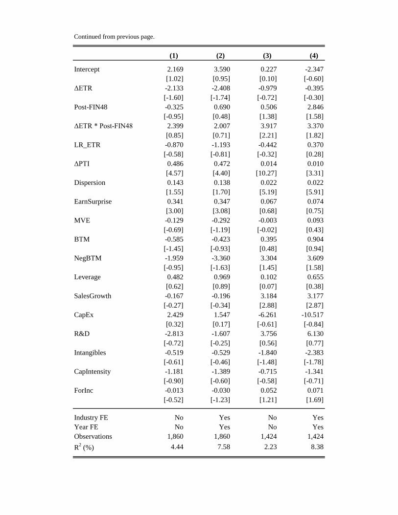
(1) (2) (3) (4)

Intercept 2.169 3.590 0.227 -2.347[1.02] [0.95] [0.10] [-0.60]

ΔETR -2.133 -2.408 -0.979 -0.395[-1.60] [-1.74] [-0.72] [-0.30]

Post-FIN48 -0.325 0.690 0.506 2.846[-0.95] [0.48] [1.38] [1.58]

ΔETR * Post-FIN48 2.399 2.007 3.917 3.370[0.85] [0.71] [2.21] [1.82]

LR_ETR -0.870 -1.193 -0.442 0.370[-0.58] [-0.81] [-0.32] [0.28]

ΔPTI 0.486 0.472 0.014 0.010[4.57] [4.40] [10.27] [3.31]

Dispersion 0.143 0.138 0.022 0.022[1.55] [1.70] [5.19] [5.91]

EarnSurprise 0.341 0.347 0.067 0.074[3.00] [3.08] [0.68] [0.75]

MVE -0.129 -0.292 -0.003 0.093[-0.69] [-1.19] [-0.02] [0.43]

BTM -0.585 -0.423 0.395 0.904[-1.45] [-0.93] [0.48] [0.94]

NegBTM -1.959 -3.360 3.304 3.609[-0.95] [-1.63] [1.45] [1.58]

Leverage 0.482 0.969 0.102 0.655[0.62] [0.89] [0.07] [0.38]

SalesGrowth -0.167 -0.196 3.184 3.177[-0.27] [-0.34] [2.88] [2.87]

CapEx 2.429 1.547 -6.261 -10.517[0.32] [0.17] [-0.61] [-0.84]

R&D -2.813 -1.607 3.756 6.130[-0.72] [-0.25] [0.56] [0.77]

Intangibles -0.519 -0.529 -1.840 -2.383[-0.61] [-0.46] [-1.48] [-1.78]

CapIntensity -1.181 -1.389 -0.715 -1.341[-0.90] [-0.60] [-0.58] [-0.71]

ForInc -0.013 -0.030 0.052 0.071[-0.52] [-1.23] [1.21] [1.69]

Industry FE No Yes No YesYear FE No Yes No YesObservations 1,860 1,860 1,424 1,424R2 (%) 4.44 7.58 2.23 8.38

Continued from previous page.

TABLE 5Differential Impact of Reserves in the Post-FIN 48 Period

This table presents results of OLS regressions where the dependent variable is the abnormal filing day return,computed as the cumulative market-adjusted return over a five-day window starting on the 10-K filing day andexpressed in percentage points (Filing Return ). HiLapse is an indicator variable that equals one if the value ofLapse is above the median in a given year and equals zero otherwise. All other variable definitions are given inTables 1 and 2. The sample covers fiscal years ending 12/15/2007 to 12/31/2012, and is restricted to firms withnon-missing values for Lapse . Firms are assigned into industries based on the Fama-French 49-industryclassification scheme. t-statistics are calculated using clustered (by year-month) standard errors and are given inbrackets below coefficient estimates.

(1) (2) (3) (4)

Intercept -4.129 -4.837 -4.103 -4.727[-1.56] [-1.18] [-1.49] [-1.14]

ResEffect 0.721 0.513 -2.362 -2.214[1.66] [1.40] [-2.10] [-2.48]

HiLapse -0.103 -0.385[-0.32] [-1.39]

ResEffect * HiLapse 3.654 3.376[2.82] [3.62]

ΔETR 1.572 1.530 1.728 1.689[1.11] [0.93] [1.29] [1.11]

LR_ETR 0.722 0.205 0.710 0.237[0.48] [0.10] [0.54] [0.12]

ΔPTI 0.040 0.044 0.039 0.044[1.09] [1.29] [1.09] [1.28]

Dispersion -0.206 -0.156 -0.229 -0.175[-1.63] [-1.34] [-1.71] [-1.42]

EarnSurprise 0.191 0.167 0.176 0.154[1.08] [0.95] [0.96] [0.85]

MVE 0.359 0.587 0.358 0.587[1.69] [1.71] [1.63] [1.70]

BTM -0.021 0.240 -0.017 0.242[-0.03] [0.29] [-0.02] [0.29]

NegBTM -0.380 -1.125 -0.310 -0.935[-0.34] [-1.14] [-0.27] [-0.97]

Leverage -0.477 -1.214 -0.464 -1.291[-0.53] [-1.14] [-0.48] [-1.16]

SalesGrowth -0.001 0.115 -0.003 0.122[0.00] [0.24] [-0.01] [0.25]

CapEx 1.990 9.061 1.491 8.585[0.40] [0.85] [0.29] [0.80]

R&D 5.494 4.913 5.112 5.806[1.01] [1.41] [0.92] [1.59]

Intangibles 0.888 -0.682 0.844 -0.662[1.22] [-0.67] [1.30] [-0.67]

CapIntensity 0.415 -0.808 0.437 -0.854[0.23] [-0.29] [0.25] [-0.31]

Foreign Income 0.093 0.085 0.145 0.133[2.16] [2.22] [4.37] [4.61]

Industry FE No Yes No YesYear FE No Yes No YesObservations 1,143 1,143 1,143 1,143R2 (%) 3.91 9.24 4.61 9.86

Continued from previous page.