Value Relevance of Comprehensive Income and Its Components:

Evidence from Major European Capital Markets

Stephen W. Lin*

Florida International University

And

Olivier J. Ramond**§

Jean-François Casta***

Universite of Paris Dauphine, Paris, France

February 2007

*Stephen W. Lin is based in the School of Accounting, College of Business Administration, Florida International University, University Park, Miami, Florida 33199. E-mail : lins@fiu.edu **, *** both Olivier J. Ramond and Jean-François Casta are based in the University of Paris, Dauphine, Place du Maréchal de Lattre de Tassigny, 75016 Paris, France. Their respective contact email address are: olivier.ramond@dauphine.fr and jean-francois.casta@dauphine.fr § Corresponding author The authors gratefully acknowledge financial support from the Europlace Institute of Finance (EIF), Euronext Fundation. This research is part of the EIF project “On the Relevance of Reporting Comprehensive Income under IAS / IFRS”.

Value Relevance of Comprehensive Income and Its Components:

Evidence from Major European Capital Markets

Abstract

This study investigates the extent to which three key summary accounting income figures, namely operating income, net income and comprehensive income, provide value-relevant information to investors in Germany, France, Italy, Spain and the UK. Using a large sample over the pre-IAS-compliance period 1992-2004, we find that all these three accounting income measures are statistically associated with share returns in any of the countries under analysis although our results show some disparities in the degree of ‘usefulness’ across country samples. Our main results are then threefold. We first provide evidence that comprehensive income is less value-relevant than both the bottom-line and operating income figures in all the sample countries. Second, our results show that aggregate other comprehensive income (or dirty surplus flow) is value-relevant and provides incremental price-relevant information beyond net income in most of the sample countries. This finding is rather different from the existing literature based in the US and UK that suggests other comprehensive income is generally not value-relevant especially when it is not separately disclosed in financial statements. Finally, we find that increased transparency on reporting other comprehensive income in financial statements as required by the UK (FRS3) and US (SFAS130) accounting standards may have warranted a stronger statistical association between firm share returns and comprehensive income. This last finding therefore strongly supports the ideology underlying the IASB/FASB joint project on ‘Performance Reporting’, and also provides evidence supporting Beaver’s (1981) and Hirst and Hopkins’ (1998) psychology-based financial reporting theory. Keywords: Value-relevance, comprehensive income, other comprehensive income,

performance reporting JEL Classification: M41, G12, G31 Data availability: All data are available from sources outlined in the text.

__________________________________

1

Value Relevance of Summary Accounting Income Measures:

Evidence from Major European Capital Markets

1. INTRODUCTION

In October 2003, the International Accounting Standards Board (IASB) and the US

Financial Accounting Standards Board (FASB) (collectively, the Boards) formed a Joint

International Group (JIG) whose objective is to lead up to a project that could establish new

international accounting standards on reporting financial performance. This project was

initially entitled “Performance Reporting: Reporting Comprehensive Income1, and is mainly

concerned with the presentation and disclosure of financial performance information in

financial statements under the current international and US GAAPs. As stated by the Boards,

the financial reporting standards resulting from this project would intend:

“to establish standards for the presentation of information in order to enhance the usefulness of that information in assessing the financial performance and financial position of an entity” (IASB, Project Overview, 25th of October 2004).

Accordingly, any standards derived from this project will introduce the first generally

recognised principles on reporting financial performance into the IFRS accounting

framework. As argued by some academics and professionals (e.g. Linsmeier et al, 1997;

Barker, 2004), this project is especially well-timed because the proliferation of alternative and

inconsistent financial performance measures are prejudicial to high-quality financial

reporting, which is not only essential to any well-informed investment decisions but is also

propitious to efficient capital markets.

Although limited to the technical display of certain accounting items and measures in

financial statements, this project has indirectly induced a great controversy while enforcing

IAS-complying firms to disclose in their financial statements a highly divisive accounting

figure named ‘comprehensive income’ under the US and UK GAAPs. According to the

FASB’s Statement of Financial Accounting Concepts N°6, Elements of Financial Statements

(1985), ‘comprehensive income’ (also called ‘all-inclusive income’ or ‘clean-surplus

income’) is defined as “the change in equity [net assets] of a business enterprise during a

2

period from transactions and other events and circumstances from nonowner sources. It

includes all changes in equity during a period except those resulting from investments by

owners and distributions to owners” (SFAC No. 6, paragraph 12). Comprehensive income

differs from the traditional bottom-line or net income measure as it encompasses dirty surplus

items, often termed ‘other comprehensive income’ (OCI) by standard-setters, i.e. the

accounting items that are directly taken to shareholders’ equity and bypass the income

statement. They currently include, under IAS, foreign currency translation gains and losses,

actuarial gains and losses, and asset revaluations.

Consistent with this ‘all-inclusive’ view of income, the IASB’s Exposure Draft of Proposed

Amendments to IAS 1 ‘Presentation of Financial Statements’, issued in March 2006, first time

in history introduces the concept of ‘total recognised income and expense’, defined as “the

change in equity of an entity during a period from transactions and other events other than

those resulting from contributions by and distributions to equity holders in their capacity as

equity holders” (IASB, 2006, BC 17: 78). As a consequence, this newly promulgated

accounting item does not only directly make echo to a US old-fashioned terminology of

‘Comprehensive Income’2 but also extend a long-history debate on the current operating and

all-inclusive concept of income into the EU from the US. Before this change, European firms

did not pay much attention to this grey area of financial reporting.

The opponents of comprehensive income argue that there are two main issues in relation to

dirty surplus accounting under the current IASB proposal. First, OCI items may mis-measure

firm performance and value (Barker, 2004) and worsen agency problems because it could

make earnings manipulation by managers much easier (Robinson, 1991; CFA Institute, 2005).

A more alarming consequence is to reduce the informativeness and quality of accounting

numbers (Cope, Johnson and Reither, 1996). Second, individual dirty surplus items are

mainly determined by local accounting standards from which managers will have certain

degree of discretion over these items. Since various dirty surplus items may be recognized by

different countries due to their nation’s unique legal, cultural, institutional, and social

environment, it hinders the use of accounting numbers, especially net income, in cross-

country comparisons and threatens investors’ understanding of accounting information

reported by international firms (Linsmeier et al, 1997; CFA Institute, 2005). It could also

reduce the credibility of accounting information. In its famous 1993 report entitled ‘Financial

Reporting in the 1990s and Beyond’, the Chartered Financial Analysts (CFA) Institute3, one

3

of the largest and most influential international financial statement user groups, argue that

“We have profound misgivings about the increasing number of wealth changes that elude

disclosure on the income statement. Yet individual items may be interpreted differently. That

calls for the display of comprehensive income that allows components of different character

to be seen and evaluated separately.” (AIMR, 1993: 63). In a similar vein, the CFA Institute

recently maintained its thought arguing “To be useful in making the(se) assessments [of a

company’s economic resources, the claims to those resources and changes in them, including

measures of an entity’s performance], reported information must be timely, accurate,

understandable, and comprehensive. The financial statements must recognize, as they occur,

all events or transactions that affect the value of the company’s net assets and, hence,

common shareowner’s wealth.” (CFA Institute, 2005: 10).

On the other hand, supporters of dirty surplus accounting have repetitively justified this

practice on the grounds that it helps produce a finer performance measure that is based on

‘normal operations’ and has predictive ability (Kiger and Williams, 1977; Black, 1993; Brief

and Peasnell, 1996). In the same streamline of thoughts, Black (1980; 1993) contents that

financial statement users including analysts, stockholders, creditors, managers, tax authorities

and even economists really want an earnings figure that measures value, not value creation.

Accordingly, one of the major issues raised by the IASB project deals with whether the

format of reporting financial performance makes any difference in an efficient capital market.

This question is of much interest for small investors than those well equipped investors such

as institutional investors because sophisticated investors can obtain the information they need

through different information channels, such as direct communication with firm managers.

Reporting financial performance practice for publicly listed companies is crucial because it

could reduce information asymmetry between firm managers and investors (Leuz and

Verrecchia, 2000; Bushman and Smith, 2001), which in turn would affect international capital

allocations (Ball, 1995). However, very little effort has been made so far to evaluate the

economic consequences of reporting financial performance in the literature. As a result, it is

widely believed that the Boards need more care while setting a standard for this purpose

(Barker, 2003; 2004).

To evaluate the potential economic consequences of regulating reporting financial

performance practice worldwide, this study uses a large international sample to provide some

preliminary evidence on the usefulness of the key summary financial performance measures

4

that are most concerned by the users of account especially investors. Most of the previous

studies in this area have largely focused on UK and US stock markets. It also has become an

important issue for many countries in the world especially in continental Europe because all

the publicly listed firms in European stock exchanges hade to adopt the International

Accounting Standards since the 1st of January 2005. This study uses panel data from five

major EU countries and investigates the extent to which three key summary financial

performance measures, including operating income, net income, and comprehensive income,

provide value relevant information for investors’ decision making before the adoption of the

International Accounting Standards. This research design allows us to enhance our

understanding of the usefulness of various income measures among countries with different

legal, social, and economic environment. In addition, our empirical results may help the

Boards in evaluating whether summary financial performance measures should be disclosed

in financial statements, and whether comprehensive income provides any incremental value

relevant information for investors and should be legitimately introduced into the new coming

international accounting standards, given the importance of decision relevance of accounting

information addressed in the IASB 1989 Conceptual Framework, and eventually supersede

the traditional net income figure.

The remainder of the paper proceeds as follows. Section 2 discusses prior research. Section 3

develops the testable hypotheses. Section 4 and 5 describes our sample selection criteria and

research models, respectively. Empirical results are reported and discussed in section 6.

Robustness tests are performed and discussed in section 7. Final section summarizes and

concludes.

2. PRIOR STUDIES

Since the seminal work on earnings components by Easton and Harris (1991) and Amir,

Harris and Veuti (1993), value-relevance research has been widely recognized while

analysing the usefulness and the informativeness of accounting figures (Barth, Beaver and

Landsman, 2001). However, some authors (see Holthausen and Watts, 2001) urged that such

studies have limited or even no implication for standard setters since they are mainly based on

research models that cannot provide any inferences for standard setting. Barth et al (2001),

however, argue that value-relevance research anchors on the use of widely accepted valuation

5

models and therefore can help assess how well accounting figures reflect information used by

equity investors in their economic decisions, and accordingly provides insights into questions

of interests to standard setters. More specifically, in an international accounting standards

context, this approach can be justified on the ground that the IASB 1989 Conceptual

Framework requires that “information must be relevant to the decision-making needs of

users”, i.e. “ […] it influences the economic decisions of users by helping them evaluate past,

present or future events or confirming, or correcting, their past evaluations” (IASB,

Conceptual Framework, 1989, par. 26). Moreover, many empirical studies have used this

research methodology to examine the value-relevance of various summary accounting income

figures including comprehensive income in the US and UK. These studies can be divided into

two categories, that is, US SFAS 130 comprehensive income-based studies and the studies

dealing with US SFAS 130 comprehensive income alike outside the US4.

Most of the previous studies in this area are based in the US. Using a large US sample over

the pre-SFAS 130 period 1972-1989, Cheng et al (1993) find that both conventional summary

accounting income measures, i.e. operating income and net income, dominate comprehensive

income in terms of the explanatory power of earnings for returns. They also report that

differences between net income and operating income i.e. non-operating items, including

exceptional and extraordinary items provide incremental value-relevant information beyond

operating income. Nevertheless, Cheng et al (1993) fail to find any statistical significance for

the difference between net income and comprehensive income, i.e. dirty surplus items. Using

US data for the period 1995-1996, Dhaliwal et al (1999) re-examine this issue by

investigating the value-relevance of comprehensive income and its major three components as

required by SFAS 130. They find that the only component of comprehensive income that

improves the association between income and return is the marketable securities adjustment.

Further evidence suggests that this finding is driven by financial firms. As a result, they

conclude that comprehensive income does not provide significant value-relevant information

beyond net income.

Chambers et al (2006), however, argue that the weak results documented in the previous

studies are caused by significant measurement errors in the examined variables. This is

because US firms were not required to report the actual amounts of comprehensive income

and its components in financial statements before SFAS 130 became effective in 1997.

Researchers therefore needed to estimate these items with potentially significant measurement

6

errors before 1997. Chambers et al (2006) define the ‘estimated’ comprehensive income as

‘as if comprehensive income’ to be distinct from the ‘as reported comprehensive income’ that

is the actual comprehensive income reported in the financial statements5 after the SFAS 130

became effective in 1997. The latter income figure can only be obtained through hand

collection.

Chambers et al (2006) find that other comprehensive income and its components, including

foreign currency translation gains/losses, marketable security adjustments, and pension

liability adjustments, are never priced by the market in the pre-SFAS 130 period (1994-1997),

but are positively priced in the post-SFAS 130 period ((1998-2001) for their S&P 500 index

firms. They conclude that as reported comprehensive income and its components are price-

relevant, and provide incremental price-relevant information beyond net income although net

income still dominates comprehensive income in predicting future net income and operating

cash flow. In a very similar study, using a sample of NYSE firms during the pre-(1994-1996)

and post-(1998-2003) SFAS 130 period, Kanagaretnam et al (2005) find evidence that as if

comprehensive income and its components are all value-relevant for non-financial firms

although the post-SFAS 130 sample exhibits much stronger statistical associations. In

addition, they confirm that net income dominate comprehensive income as a predictor of

future firm operating performance. Using as if comprehensive income and its components,

Biddle and Choi (2006) find consistent results supporting the value-relevance of

comprehensive income and its components after controlling for prior year comprehensive

income. They also find comprehensive income dominates net income in predicting future net

income and operating cash flow.

Several studies have used international data. Using a small UK sample, O’Hanlon and Pope

(1999) find that dirty surplus components are not price-relevant except extraordinary items

even when using various measurement intervals. In the UK Financial Reporting Standard

N°3 (1993) context, Lin (2006) find dirty surplus items such as extraordinary items, foreign

currency translation gains/losses, reversal of written goodwill, and other items are all value-

relevant and provide incremental value-relevant information beyond net income using UK

data for the period 1993-1998. Using a small New-Zealand sample, Cahan et al (2000) do not

find any evidence on the value-relevance of comprehensive income and its components.

Similarly, using Australian data over the period 1988-1997, i.e. the pre-AASB N°1018

‘Statement of Financial Performance’ period, Brimble and Hodgson (2005) document that

7

comprehensive income exhibit lower value relevance than net income, and that dirty surplus

components have very minor price information content even after considering non-linear

setting.

In summary, previous empirical evidence on the value-relevance of comprehensive income

and its components are generally mixed. Interestingly, all these studies are based in English

Speaking countries where Anglo-American accounting system dominates. The main features

of this accounting system are principles-based and equity capital market-oriented. Managerial

discretion over accounting recognition and disclosure has played an important role under this

accounting system. It is likely that managerial discretion over the recognition of

comprehensive income and its components may have significantly reverse effect on their

potential link with firm value. In contrast, continental European countries such as Germany

and France adopted a more rules-based and credit capital market- and tax-oriented accounting

system, where managerial discretion has played a less important role in deciding

comprehensive income and its components. Investors may be able to understand and correctly

use the information in a more efficient and effectively way in these countries. Hence, using a

large sample firms from five major European countries this study provide further empirical

evidence on the value-relevance of comprehensive income and its components, underlying the

IASB / FASB joint project on ‘Performance Reporting’. Research hypotheses are discussed

next.

3. HYPOTHESES DEVELOPMENT

The hypotheses developed in this section refer to the IASB/FASB ‘Performance Reporting’

joint project and the literature regarding the value-relevance of comprehensive income and its

components. More precisely, we focus on the following four major issues which underlie the

debates surrounding the above joint project:

1) Are comprehensive income and its components value-relevant?

2) Does comprehensive income, at an aggregate level, provide incremental value-relevant

information beyond net income and operating income?

3) Does ‘other comprehensive income’ provide incremental value-relevant information

beyond traditional net income?

8

4) Can we observe differences in value-relevance between ‘reported comprehensive income’

and ‘non-reported comprehensive income’? In other words, is ‘comprehensive income’

more value-relevant when it is clearly disclosed on the face of the financial statements

than when it is not?

Different from the previous studies, we investigate the above issues using international data

because we believe the value relevance of comprehensive income and its components could

be conditional on a nation’s unique socio-economic environment. We predict that the value

relevance of comprehensive income and its components is different between countries where

the principles (or market-oriented) or rules (or credit-oriented) based accounting systems are

used respectively.

The above four issues are investigated in this study through the following five hypotheses.

Under the IAS, European firms were previously required to clearly identify and disclose both

operating profit6 and its components on the face of the P&L if they are material (IAS1 v2003,

par. 75; the IASB Conceptual Framework, pars. 29-30). Although operating profit has not

been clearly defined in any international accounting standard, the IASB regards it as an

important income summary measure (IAS 1 v2005, BC 12 and 13). If the IASB standard-

setter is correct in the assessment of the decision relevance of operating income, then the

following hypothesis should be true.

H01: operating profit is value- relevant and provides incremental value-relevant

information beyond net income

Comprehensive income and dirty surplus items have been at the centre of one of the major

accounting debates among accounting profession and academia for several decades. As

discussed earlier, this debate involves two very different concepts of accounting income, that

is, current operating and dirty surplus accounting. Analysts have regularly expressed

dissatisfaction not with what is reported in the present-day statements of income, but rather

with what is not reported in them (CFA Institute, 2005). More specifically, their discontent is

about the present practice of directly taking certain items of comprehensive income to equity

(Foster and Hall, 1996). For example, in its 1993 report, the CFA Institute argued that there

seems no conceptual basis for allowing certain accounting items to be directly taken to equity

and bypass the income statement. Since these items are not currently included in the statement

9

of income or financial performance, the accounting treatment for comprehensive income and

its components is still not determined. In addition, without a sound reporting of the ‘all-

inclusive’ earning through a dedicated statement “much effort is required of analysts to locate

and evaluate all of the income statement items that can have a bearing on their forecasts of the

future and the valuation of the firm” (CFA, 2005: 10).

Opponents of dirty surplus accounting, however, assert that excluding transitory items from

earnings help investors’ valuation process. Skinner (1999) argues that empirical studies have

for the most part failed to provide evidence that other comprehensive income has implications

for a firm’s future operating performance or cash flows. He also argues that other

comprehensive income mainly include “accounting adjustments that are difficult to interpret

economically and which sophisticated analysts tend to ignore in estimating future earnings

and cash flows”. Similarly, White et al (1998, quoted in Skinner, 1999) conclude these items

add undoubtedly noise to reported earnings and are therefore meaningless in any valuation

process.

Following Skinner’s (1999) claims, one may expect that comprehensive income is less value-

relevant than other conventional summary income figures since investors are more interested

in using recurrent earnings for valuation purpose. On the other hand, CFA Institute (2005)

argues that dirty surplus items are important information that is absolutely necessary for the

securities analysis and valuation purposes. As a result, the above two competing theories can

be empirically verified through the following hypothesis:

H02: Comprehensive income, at an aggregate level, is value-relevant and

provides incremental value-relevant information beyond net profit and

operating profit.

Some FASB and IASB board members overtly claim that investors and other users of

accounts have over emphasized net income and earnings per share (see for instance, Foster

and Hall, 1996). They, however, believe that “if the components of comprehensive income

become more transparent, analysts and other users of financial statements will be more likely

to focus on those individual components in evaluating the quality of earnings and in assessing

the likelihood that past reported income can be used to forecast future financial performance”

(Foster and Hall, 1996: 19). In this respect, it has been argued that “the new figure [i.e.

10

‘comprehensive income’] will shine a bright, embarrassing light on items that are now buried

in shareholders’ equity” (MacDonald, 1997) and will permit to measure and recognize the

economic activities and events affecting a company’s operations (CFA, 2005).

In parallel of the above normative claims, psychology-based financial reporting research that

focuses on the presentation and display of accounting information document that financial

statement users are more likely to use information when it is provided in a clear, simple

manner (e.g. Johnson, Payne, and Bettman, 1988; Harper, Meister and Strawser, 1987, 1991).

In this sense, Hirst and Hopkins (1998: 1) note: “research in psychology suggests that

information will not be used unless it is both available and readily processable (i.e. clear)”.

Similarly, Beaver (1981) carves out the rationale of accounting regulation under the efficient

market hypothesis stating that if accounting regulation makes the market more efficient with

respect to a richer information set, then the price effects may be expected as a result of

accounting disclosures. Consistent with this analysis, Sanbonmatsu et al (1997) find evidence

that if individuals perceive information to be more important (e.g. other comprehensive

income and its components, may be perceived to be more important once they are disclosed as

part of comprehensive income), they weight this information more heavily in their decision

making if the informational environment is finer7.

From an EU standard-setting point of view, disclosure of comprehensive income is already

required in the UK since 1993. Indeed, UK FRS 3 “Reporting Financial Performance”, first

issued in October 1992, explicitly requires the reporting of a comprehensive income item

through the Statement of Total Recognized Gains & Losses (hereafter, STRGL). The STRGL

is defined by FRS 3 as “a primary financial statement that includes the profit or loss for the

period together with all movements in reserves reflecting recognised gains and losses

attributable to shareholders” and therefore looks quite similar to the Statement of Total

Recognized Income and Expense (STRIE) promulgated by the IASB IAS 1 amendment.

Therefore, following Beaver (1981) and Hirst and Hopkins (1998), the following hypothesis

is expected to be empirically verified:

H03: Comprehensive income is more value-relevant, and provides more

incremental price information beyond net income in the UK than any other

continental European countries.

11

As shown previously, proponents of reporting comprehensive income include the CFA

Institute, one of the largest and most influential user groups. As depicted in its 1993 report,

the CFA Institute believes comprehensive income is needed for better and more useful

financial reporting in several areas, including reporting the impact of changing in fair values

of marketable securities and all other non-owner changes in equity that currently are reported

as equity adjustments. Stepping the CFA’s proposals and the US SFAS 130 disclosure

requirements, the IASB issued in March 2006 an amendment draft focusing on the disclosure

of a firm’s other comprehensive income providing that it is value-relevant and provides

incremental value-relevant information beyond net income. If the authors of the IAS 1

amendment draft are correct, the following hypothesis should be true:

H04: Other comprehensive income is price-relevant and provides incremental

price information beyond net income.

Again, following the psychological finding suggested by Hirst and Hopkins (1998) and the

disclosure theory suggested by Beaver (1981), we predict the information contained in dirty

surplus in the UK should be reflected into share price better than other continental European

countries due to the fact that the STRGL has been required by FRS3 since 1993. As a result,

the following hypothesis is expected to be empirically verified:

H05: Other comprehensive income is more price-relevant and provides more

incremental price information beyond net income in the UK than in any

other European country.

The value relevance of accounting information has been widely examined through the

statistical association between share return and accounting numbers in the accounting

literature. In other words, one possible economic consequence of accounting information

disclosure is directly linked to the change in share price. Following Roll (1988) and Lev

(1989), this study uses the explanatory power of examined accounting items for share returns

(i.e. R² statistic) to investigate their usefulness8 for investors (or the capital market overall)

and a way to test the previously developed hypotheses.

12

Using a large sample from European listed firms obtained from DATASTREAM and

WORLDSCOPE databases, we examine the information set perspective of IASB

“Performance Reporting” Project through the above five hypotheses. The details of sample

selection and data collection are summarised in section 5. The next section describes the

major steps of the research design methodology.

4. RESEARCH DESIGN

Our research design to investigate the above five hypotheses is briefly discussed as follows.

(i) Comprehensive income and other comprehensive income

In European countries, including the five countries under analysis in this study (i.e. UK,

France, Germany, Italy, and Spain), dirty surplus accounting items and practices vary widely

from one national accounting framework to another one. Since it would be too costly to deal

with country-specific dirty surplus components, we choose to use a proxy for other

comprehensive incomes inspired from the Ohlson’s (1991) clean surplus relationship. The

articulation between balance sheet amounts, accounting flows, dividends and capital changes

for each accounting period, t, is then defined as follows (company subscript suppressed):

1t t t t tV BV N d CI−≡ + − + B (1a)

t

t (1c)

) and (1b), it is

traightforward to rewrite these two latter equations respectively as follows:

Or: (1b) t t tCI BV N d≡ ∆ − +

Where ∆ denotes a change between periods t-1 and t; BV denotes the book value of ordinary

shareholders’ funds; N denotes the firm’s total equity issued; d denotes annual cash dividends

and CI denotes the firm’s comprehensive income. Moreover, since comprehensive income is

defined here as an ‘all inclusive income’, it can be stated that:

t tCI NI DS≡ +

Where NI denotes the firm’s bottom-line income (or net income) and DS denotes dirty surplus

items or other comprehensive income. Substituting expression (1c) into (1a

s

13

BV BV N d E DS−≡ + − + +1t t t t t t (1d)

[ ] [ ]t t t t tDS BV N E d≡ ∆ − − − (1e)

s accounting flow9. These proxies

ill be used in the research models described hereafter.

Modelling background

Where [∆BVt – Nt] represents the movement of shareholders’ funds and [Et – dt] denotes the

annual income that the firm decides to reintroduce in its cyclical activities (i.e., the “firm self-

funding item”; see Beaver (1981)) for the accounting period t. Relationship (1e) does

underline that there are three important flow statements underlying the IASB project like in

UK FRS 3 (that does not include the balance sheet). [Et – dt] appears in the profit and loss

account (which constitutes a sub-statement in the IASB project), change in BV and change in

capital appears in the reconciliation of the movements in shareholders’ funds (called in the

IASB project, ‘statement of changes in equity’); DS appears in the STRIE (i.e. the statement

of comprehensive income). Therefore, equations (1b) and (1e) provide proxies respectively

for comprehensive income and for the yearly dirty surplu

w

(ii)

onsiders

n Ohlson (1995)-based model taking the following form for each financial period t:

The idea that market capitalization and book value are closely related to each other as being

the two faces of the same coin of shareholders’ equity “stock” values has been widely

documented in the financial literature in the past two decades (e.g. Harris and Ohlson (1987);

Lev (1989); Easton and Harris (1991)). However, links observed between share price,

earnings, dirty surplus and other movements in shareholders’ funds have seldom been

formerly demonstrated. In a UK earnings-return association study, Lin (2006) proposes an

Ohlson (1995) model-based approach to examine the above relationships. We thus c

a

( ) (1 )t t t tP k CI d k BV Vtϕ α= − + − + (2)

Where P denotes the firm’s share price at time t; CI denotes comprehensive income per share,

d is the firms’ annual dividend per share; V denotes additional information about future

earnings that is not reflected in current earnings and book value for period t; k is a factor for

weighting the contribution of change in book value, i.e. φCI – d, versus book value levels in

14

the explanation of stock price, and φ, α are other estimated parameters. As underlined by

Ohlson (1995), this valuation model states that a firm value is a weighting sum of a book

alue model, i.e. tBV , and an earnings model, i.e. t tCI dϕ −v .

turn-

arnings relationship literature (e.g. Easton & Harris (1991); O’Hanlon & Pope (1999)):

A more simplified form of the above model has frequently been investigated in the re

e

0 1 2t t t tP BV CIα α α ε= + + + (3)

Where P denotes the firm’s share price adjusted for dividend, BV denotes the firm’s book

value per share, CI denotes the firm’s comprehensive income (or earnings) per share and the

t t denotes the accounting period.

le.

odel (3), expressed for every financial period t, is then transformed to:

subscrip

To avoid encountering scale effect in the return-earning regression statistics, some previous

studies (e.g. Cheng et al (1993); Easton (1999)) have proposed another modelling

specification that turns the dependent variable, i.e. share price P, into a share return variab

Following this, m

0 1 21 1t t

t tt t

CI CIRET uβ β β ∆= + + +

Using the relationship (1c), it is

ightforward to rewrite (4) as:

P P− − (4)

Where RET is the firm’s average cumulative share return10, P is the firm’s cum-dividend

share price, CI is comprehensive income per share and ∆CI is the change in comprehensive

income per share during each accounting period t.

stra

0 1 21 1

t t t tt t

t t

NI OCI NI OCIRET uP P

β β β− −

+ ∆ + ∆⎛ ⎞ ⎛ ⎞= + + +⎜ ⎟ ⎜ ⎟⎝ ⎠ ⎝ ⎠ (5a)

Or

0 1 1 2 21 1 1 1

t t t tt t

t t t t

NI OCI NI OCIRE

is noteworthy that following Ohlson’s (1989; 1995) framework, the assumption on the

coefficients of CI, i.e.

T uP P P p

β β β β β− − − −

∆ ∆= + + + + +

(5b)

It

1β and 2β , might not be verified given earnings reported in the profit

15

and loss account have higher persistence than dirty surplus items that are reported in the

statement of total recognised incomes and expenses (Pope and Wang, 2005).

Similarly to Ohlson (1999) and Pope and Wang (2005), we propose to investigate the

following extended model that allows for more flexible considerations:

tt

t

t

t

t

t

t

tt u

pPPPRET '

14

13

12

110 +++++=

=−−−γγγγγ

(5

OCIOCININI ∆∆

c)

e value-relevance of each earnings

ponent. The following subsection presents the research approach adopted in this study.

Model (5c) is then further developed to investigate th

com

(iii) Value -Relevance Models for Earnings Components

Consistent with Lin’s (2006) and Cheng et al’s (1993) methodologies, comprehensive income

(or earnings) in model (5b) is then decomposed into the typical functional P&L structure. To

ompare the information content between three different summary measures of financial

erformance and test our (5c) for each key performance

easure and its components, and for each of our five country sam

c

p five hypotheses, we estimate model

m ples:

' ' 't tOPIN OPINET '0 1 2

1 1t t

t tR

P Pγ γ γ ω∆

= + + +− −

(6a)

'' '' '' ''0 1 2

1 1t t

t tt t

NI NIRETP P

γ γ γ ω∆= + + + (6b)

− −

(3) (3) (3) (3)0 1 2

1 1

t tt t

t t

CI CIRETP P

γ γ γ− −

∆= + + + ω (6c)

tt

t

t

t

t

t

t

ttRET

pOCI

POCI

PNI

PNI

ωγγγγγ +∆

++∆

++==−−− 1

)4(4

1

)4(3

1

)4(2

1

)4()1(

)4(0 (6d)

formulated into the following five null hypotheses:

01: R²NI|OPIN ≡ R²NI - R²OPIN = 0

Accordingly, our five hypotheses can be re

H

H02: R²CI|NI ≡ R²CI - R²NI = 0

H03: R²NI,DS|NI ≡ R²NI,DS - R²NI = 0

16

H04: R²CI(UK)|CI(EU) ≡ R²CI(UK) - R²CI(EU) = 0

05: R²NI,DS(UK)| NI,DS(EU) ≡ R²NI,DS(UK) - R²NI,DS(EU) = 0

ere R²P|Q denotes an increase in adjusted-R² due to variable P, conditional on variable Q

H

Wh

and R²P,Q denotes the adjusted-R² due to P and Q11.

(iv) Nested and non nested statistical tests

Following previous studies, whether earnings components and dirty surplus items provide

incremental value-relevant information over aggregate earnings is measured by the difference

in adjusted R-squared values between nested models and its statistical significance (using F-

test), and the statistical significance of the slope coefficients of examined variables. In the

ase of non-nested models’ comparison, the likelihood-ratio-based Vuong’s (1989) test is

verwhelming R-squared values in price-level regressions. This study uses only share returns

ssociated with panel data and therefore should not encounter this peculiar econometrical

issue.

ur four continental European countries. We therefore leave the value-relevance of

omprehensive income after the adoption of the international GAAPs for future research.

c

implemented. Easton and Sommers (2003) document that the scale effect gives rise to

o

a

The details of sample selection and data description are shortly discussed in the next section.

5. SAMPLE SELECTION AND DATA DESCRIPTION

We initially collected accounting data for all the listed companies on the UK, German,

French, Italian and Spanish stock markets available from DATASTREAM and

WORLDSCOPE for the period 1992-200412. Since the international accounting standards are

effective in EU from 2005 onwards, we do not include this year in the sample. This is

because we believe the content of comprehensive income and its components may have been

changed due to the accounting differences between the international GAAPs and national

GAAPs in o

c

Using the level 6 industrial classification in DATASTREAM, coded INDC613, we deleted

sample observations with INDC6 spanning from 8000 to 8999 (i.e. financial sectors). We

17

exclude these firms because of their unique regulatory environment and financial reporting

practice.

‘Comprehensive Income’ is not clearly reported on the face of financial statements during the

st period in four of our five sample countries, including Germany, France, Italy and Spain14

although the information to l statements15.

either DATASTREAM nor WORLDSCOPE provide a separate item for comprehensive

t (1b)

t

f period t; N denotes new equity issued during period t; and d denotes dividends paid to all

ts use the following accounting items in DATASTREAM

odel 1(b):

ata in DATASTREAM or WORLDSCOPE were

eleted from the sample. We also excluded firms whose financial markets data are not

available in DATASTREAM potential outliers on

ur empirical results, we deleted top and bottom 1% extreme observations for each variable of

terest. Table 1 exhibits a breakdown by country of the sample size before and after deleting

outliers for each model used in t

TABLE 1 ABOUT HERE]

te

construct it is readily available from financia

N

income16. Subsequently, we manually computed comprehensive income using the following

well-known clean-surplus formula17:

t t tCI BV d N≡ ∆ + −

Where BV denotes the book value of ordinary and preference shareholders’ funds at the end

o t t

shareholders during the year.

More precisely, our empirical tes

and WORLDSCOPE to construct the variables in m

BV ≡ Ordinary Share Capital (Item #301) + Reserves (Item #304)

+ Preference Capital (Item #306)18

d ≡ Dividends Paid (Item #434)

N ≡ Total Equity Issued (Item #406)19

As a result, firms with missing accounting d

d

. Besides, in order to avoid the impact of

o

in

he analysis.

[INSERT

18

6. EMPIRICAL RESULTS

(i) Univariate and bivariate statistics

The descriptive statistics of all the variables examined in this study are reported in Table 2.

Accounting variables are reported on a per share basis, and are deflated by prior year end

share price. Panel A shows that the mean (median) value of comprehensive income is -0.010

(0.041) in the UK, -0.018 (0.024) in Germany, 0.032 (0.049) in France, 0.023 (0.036) in Italy

and 0.092 (0.069) in Spain, respectively. The mean (median) value of net income is -0.021

(0.049) in the UK, -0.036 (0.032) in Germany, 0.033 (0.052) in France, 0.008 (0.038) in Italy

and 0.061 (0.070) in Spain, respectively. Net income appears to be smaller than

comprehensive income except in France. The Mann-Whitney-Wilcoxon two-tailed test shows

that comprehensive income (CI) and net income (NI) are significantly different except in

Spain and Italy. We further examine the distribution of the other comprehensive income

(OCI) in these two countries. Unreported Student’s t-test shows that OCI in the Italian and

panish samples is statistically different from zero at a 1% level. We therefore expect that

Panel B exhibits the Pearson ficients for all the variables

nder analysis. It shows that OCI is negatively correlated to net income (NI) and operating

except Spain, and positively correlated to

prehensive income (CI) and change in comprehensive income (∆CI).

S

both NI and CI provide different value-relevant information amongst the examined samples.

Spain has the highest amount of OCI (i.e. 3.10%) in comparison with UK, (1.20%), Germany

(1.70%) and Italy (1.50%). France is the only country with very small negative OCI

(i.e. -0.10%)

and Spearman rank correlation coef

u

income (OPI) for all the examined countries20

com

[INSERT TABLE 2 ABOUT HERE]

(ii) Price relevance of performance components

Unreported Shapiro-Wilks statistics show that most of the examined performance components

are not normally distributed, indicating that potential outliers might still drive the OLS

statistics. To overcome this problem, two sets of regression results are provided for

19

comparison and robustness test purposes. The first set of results use ‘reported’ summary

accounting measures as independent variables (i.e. the conventional OLS method); the second

set of results uses the ranks of reported summary accounting measures as independent

variables (i.e. the ranking method). They are reported in Panels A and B, respectively

roughout Tables 3 to 6. The ranking method, inspired from Fama and McBeth’s (1973)

the 1% level,

uggesting operating income is indeed value relevant; (3) slope coefficients are consistently

summary, results reported in Table 3 suggest that operating income is value relevant in all

the examined countries altho or investors in both France

nd Italy. We find evidence supporting H01 in the sense that operating income is value

th

zero-investment portfolio construction methodology, has been used in many empirical studies

(e.g. Abarbanell and Bushee, 1998; Raedy, 2000; Lin, 2006) to standardise all the explanatory

variables in order to reduce the impact of potential outliers, and to fit the potential non-linear

relationship between share return and accounting numbers better.

Panel A of Table 3 reports regression results for the value relevance of operating income

across five EU countries. Results indicate that the slope coefficients of the level of and

change in operating income (OPI and ∆OPI, respectively) are value relevant in all the five

cases. However the usefulness of operating income for investors, as proxied by the regression

R-squared values, appears to vary across our sample countries. Operating income appears to

explain the variation of share return better for French and Italian firms. Theses findings are

also confirmed by the ranking OLS method reported in Panel B. Panel B shows that (1) R-

squared values are consistently higher than those using the conventional OLS method,

indicating that the ranking method fits the relation between share return and earnings

components better; (2) both OPI and ∆OPI are statistically significant at

s

lower than those using the conventional OLS method, suggesting that the ranking method

alleviates the influence of outliers; (4) R-squared value is higher for French (16.59%) and

Italian (16.62%) samples, indicating that following Lev’s (1989) framework, operating

income is more ‘useful’ in these two countries than UK, Germany and Spain.

In

ugh it appears to be more ‘useful’ f

a

relevant. Table 6 reports the evidence on whether operating income provides incremental

price information beyond net income.

[INSERT TABLE 3 ABOUT HERE]

20

Table 4 reports the results for the value relevance of net income using both the conventional

and ranking OLS regression models. It shows that net income is consistently associated with

return in all the examined countries. The level of and change in net income are statistically

significant at the 1% (5%) level in Germany, France, Italy and Spain (UK) except in Italy for

the change in net income under the conventional OLS method. Besides, conventional OLS R-

squared values are consistently higher in the French, Italian and Spanish samples, suggesting

that net income is more ‘useful’ for investors in these countries than in the UK or Germany.

In addition, it is worth noting that adjusted R-squared values of German sample in Panel A of

ables 3 and 4 appear lower than that of France, Italy and Spain. Leuz and Wüstemann

and ∆NI appear to be positively associated with share return at the

% level in all the cases. The ranking regression fits the association between share return and

net income better, and effec e observations on the OLS

gression. Using the both regressions, UK firms appear to have lowest R-squared value,

indicating that NI contains less value-relevant information in the UK in comparison with other

T

(2005) justify this finding on the ground that insider information and trading are commonly

spread on the German market due to its bank-oriented financing system. Subsequently,

private information diffusion coupled with insider trading could have reduced the

contemporaneous association of accounting numbers with share returns.

Using the ranking OLS regression, Panel B shows that (1) the R-squared values of model (6b)

ranges from 10.42% to 27.78% and are much higher than those using the conventional OLS

method (ranging from 4.88% to 14.80%); (2) the slope coefficients of level of and change in

net income (NI and ∆NI, respectively) are much smaller (except in Germany where they are

higher and in UK where they are almost equal) than those using the conventional OLS

regression model; (3) NI

1

tively reduces the impact of extrem

re

European counterparts.

[INSERT TABLE 4 ABOUT HERE]

Table 5 reports results for the value relevance of comprehensive income. Panel A of Table 5

shows that both level of (CI) and change in comprehensive income (∆CI), respectively are

positively and statistically associated with share return at least at the 5% level except Italy and

Spain where change in comprehensive income is insignificant. Panel B reports results using

the ranking OLS method. Again, we find that the R-squared values using the ranking

21

regression (ranging from 6.38% to 20.75%) are much higher than those using the

conventional OLS regression (ranging from 3.57% to 9.56%). Besides, R-squared values are

onsistently higher for German, French and Italian samples (13.55%, 14.92% and 20.75%,

respectively). In summary, e sense that comprehensive

come is value-relevant in all the examined countries. Table 6 reports the evidence on

er the post-FRS 3 period 1993-1998. It is

lso consistent with US evidence from Cheng et al (1993) that operating income is more

c

we find evidence supporting H02 in th

in

whether comprehensive income provides incremental price information beyond net income

and operating income.

[INSERT TABLE 5 ABOUT HERE]

In summary, tables 3, 4, and 5 indicate that operating income, net income, and comprehensive

income are all statistically associated with share return. It appears that net income and

comprehensive income are more useful for investors, measured by the R-squared values, for

continental European countries especially for the Latin countries, namely France, Italy and

Spain. Interestingly, UK investors do not value these two measures of income as much as

their continental European counterparts. They appear to emphasise on operating income

instead. The above findings are further confirmed in the Panel A of Table 6. It shows that the

mean and median R-squared values for all the models are consistently lower when UK

samples are included except operating income. This indicates that net income and

comprehensive income are more useful in continental European countries than UK. Operating

income appears to be the favourite measure of income for UK investors. This is consistent

with Lin (2006) who documents that operating income provide incremental price-relevant

information beyond pre-tax earnings in the UK ov

a

associated with share return than net income and comprehensive income. In summary, the

above results provide no evidence to support H03 in the sense that comprehensive income in

the UK is not as useful as that in continental European countries, and it does not provide

incremental price information beyond net income.

To further test H01 and H02, we also need to investigate whether one measure of income

dominates the other. This study uses the Vuong’s (1989) non-nested test to evaluate the

statistical difference in R-squared values from models (6a), (6b), and (6c). Panel B of Table 6

shows that comprehensive income is less value-relevant than net income at the 1%

significance level in all the cases. Besides, Vuong’s statistics also show that comprehensive

22

income exhibits less value-relevance than operating income at the conventional significance

levels in UK, France and Germany (only using the ranking regression). Consistent with our

previous finding, net income dominates operating income in Germany and Italy when using

both methods, and in France and Spain when using the ranking method only. Operating

income appears to dominate net income in our UK sample. This interesting finding could be

caused by the fact that operating income has been reported by UK firms on the face of profit

and loss account since FRS3 became effective in 1993 if it is not earlier. In contrast, European

vestors may not be familiar with this item especially when it is not defined clearly in any

does not provide incremental price information ng income for all the

examined countries. H03 is a rehensive income in the UK

not as value-relevant (useful) as it is to other European countries, and that it does not

ue-relevant and provide incremental price information beyond net income for

ll the examined countries. We also find that aggregate OCI and/or CI are value-relevant for

all the examined countries, ation beyond net income.

in

accounting standards yet. Overall, we find no evidence supporting H01 in the sense that

operating income provides incremental price information beyond net income for our

continental European countries, although there is evidence to support this hypothesis in the

UK.

Furthermore, we also find no evidence supporting H02 in the sense that comprehensive income

beyond net and/or operati

lso rejected due to the fact that comp

is

provide more incremental price information beyond net income than that in other continental

European countries. These findings are robust for both conventional and ranking regressions.

[INSERT TABLE 6 ABOUT HERE]

Table 7 reports the results for the incremental value relevance of other comprehensive income

beyond net income. Panel A shows that the level of OCI is negatively associated with share

return for Germany and France, but the change in OCI is positively associated with return for

all the countries except Spain. Again, we find that R-squared value is higher for France, Italy

and Spain. Panel B, using the ranking OLS regression, shows that the slope coefficients of

level of and change in other comprehensive income are significant at the conventional levels

after controlling for net income (except Spain where change in other comprehensive income is

not significant). Italy, France, and Germany appear to have much higher R-squared values

than UK and Spain. In summary, we find evidence on supporting H03 in the sense that dirty

surpluses are val

a

and provide incremental price inform

23

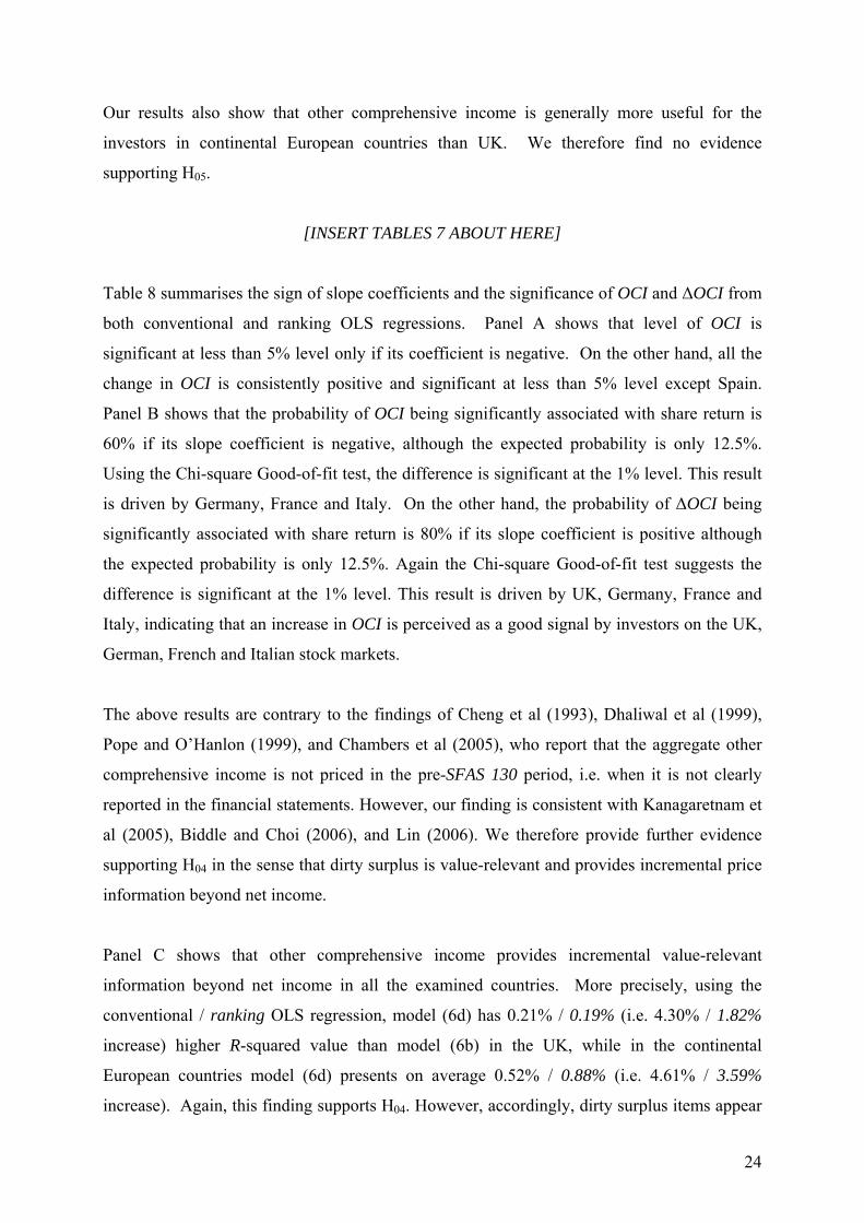
Our results also show that other comprehensive income is generally more useful for the

n the other hand, the probability of ∆OCI being

ignificantly associated with share return is 80% if its slope coefficient is positive although

Chambers et al (2005), who report that the aggregate other

omprehensive income is not priced in the pre-SFAS 130 period, i.e. when it is not clearly

1.82%

increase) higher R-squared value than model (6b) in the UK, while in the continental

European countries model .88% (i.e. 4.61% / 3.59%

increase). Again, this finding supports H04. However, accordingly, dirty surplus items appear

investors in continental European countries than UK. We therefore find no evidence

supporting H05.

[INSERT TABLES 7 ABOUT HERE]

Table 8 summarises the sign of slope coefficients and the significance of OCI and ∆OCI from

both conventional and ranking OLS regressions. Panel A shows that level of OCI is

significant at less than 5% level only if its coefficient is negative. On the other hand, all the

change in OCI is consistently positive and significant at less than 5% level except Spain.

Panel B shows that the probability of OCI being significantly associated with share return is

60% if its slope coefficient is negative, although the expected probability is only 12.5%.

Using the Chi-square Good-of-fit test, the difference is significant at the 1% level. This result

is driven by Germany, France and Italy. O

s

the expected probability is only 12.5%. Again the Chi-square Good-of-fit test suggests the

difference is significant at the 1% level. This result is driven by UK, Germany, France and

Italy, indicating that an increase in OCI is perceived as a good signal by investors on the UK,

German, French and Italian stock markets.

The above results are contrary to the findings of Cheng et al (1993), Dhaliwal et al (1999),

Pope and O’Hanlon (1999), and

c

reported in the financial statements. However, our finding is consistent with Kanagaretnam et

al (2005), Biddle and Choi (2006), and Lin (2006). We therefore provide further evidence

supporting H04 in the sense that dirty surplus is value-relevant and provides incremental price

information beyond net income.

Panel C shows that other comprehensive income provides incremental value-relevant

information beyond net income in all the examined countries. More precisely, using the

conventional / ranking OLS regression, model (6d) has 0.21% / 0.19% (i.e. 4.30% /

(6d) presents on average 0.52% / 0

24

to provide more incremental price information beyond net income in continental European

countries than UK. As a result, we cannot find evidence supporting H05.

el. Moreover, in some cases, the sign

f the coefficients are consistent with our previous finding but their statistical significance

As noted previously, many EU firms, especially German listed firms, have adopted US, UK

and international GAAPs prior to the IAS-compliance transition date because of cross-listing

regulatory requirements or accounting policy choice. This study uses the following two

ethods to investigate the potential impacts of these early adopters on our empirical results.

[INSERT TABLES 8 ABOUT HERE]

7. SENSITIVITY TEST

To investigate whether the above findings are sensitive to how share return is calculated, we

provides two robustness checks by replacing raw return in models (6a) to (6d) with abnormal

return derived from the market-adjusted and market models. Unreported results suggest that

aggregate other comprehensive income, i.e. OCI, does not appear to provide statistically

significant incremental price information beyond aggregate net income for Germany and Italy

when abnormal return is derived from the market mod

o

have been reduced, indicating that results using abnormal return appears to be weaker than

those using raw return. Finally, R-squared values using the abnormal return derived from the

market model appear to be weaker than those using the raw return and abnormal return

derived from the market-adjusted model respectively.

m

Firstly, we add an early adopter dummy variable to our regression model, shown as follows:

0 1 2 3 41 1 1 1

. . . . . .t t t tt t t t

t t t t

I I I IRET D DP P P P

λ λ λ λ λ ε− − − −

∆ ∆= + + + + + (6e)

Where RET is the firm’s average cumulative share return as defined previously; D is a dummy

ariable taking the value 1 if the company is an early adopter of IFRS and 0 otherwise; P is

the

in the

v

firm’s cum-dividend share price; I is an accounting income measure and ∆I is the change

accounting income measure (i.e. operating income, net income, or comprehensive

25

income

period

1)

an ASB in July 2005.

When data appear to differ between these two sources, we referred to the GASB

en a firm publishes its financial

statements under local GAAPs for more than two consecutive years, we presume that

ready cross-listed on the UK or the US stock market at the end of

period t. Wordscope data are double checked with the non-US listed firms listing

.

The numbers of early adopt years in Table 9. It shows

at Germany early adopters represent about 27.6% of the entire Germany sample firms, while

) during period t. More precisely, the dummy variable, Dt, takes the value 1 for the

t if the firm meets at least one of the following two criteria:

The firm must publish its financial statements under the International, US or UK

GAAPs at the end of period t. This information was originally collected from the

WorldScope database. Besides, since the German sample contains more early

adopters than any of the three other continental countries, we double checked the data

from WordlScope by referring to the reports issued by the Germ

information. Moreover, missing data is dealt with based on the following two rules:

(i) when one year data is missing between two identical year data, we assume that the

missing data is same as the collected data; (ii) wh

the firm also followed local GAAPs during the preceding years.

2) The firms are al

provided by the NYSE Group on 30th October 2006.

As a result, if the accounting income measures of early adoption firms provide incremental

price relevant information beyond those of other firms, then we should be able to observe a

significant λ1 and/or λ2

ers are presented by countries and by

th

early adopters only represent around 5% of the entire sample firms in other three European

countries. OLS regression results of model (6e) for Germany, France, Italy and Spain are

reported in Table 10.

[INSERT TABLES 9 ABOUT HERE]

Results exhibited in Table 10 indicate that only German and French early adopters have

significant impact on the regression estimators. In the German (French) sample, early

adopters impact positively (negatively) the relationship between the accounting income

26

measure (except operating income) and share return. Interestingly, we find that all the R-

squared values increase after controlling for early adopters for Germany except for the net

come model. This finding also applies to France except for the operating income model. In

contrast, Italy has higher R ve income model. All the

-squared values decrease after controlling for early adopters for Spain. As a result, we

sed by the fact that the early adopters are normally

ross-listed firms and are generally larger than the late adopters. They normally have larger

mount of aggregate other comprehensive income than the late adopters. More importantly,

our result also indicate ehensive income and its

omponents in financial statements as required by the UK (i.e. FRS3) and US (i.e. SFAS130)

in

-squared value only for the comprehensi

R

conclude that the other comprehensive income of German, French, and Italian early adoption

firms provides incremental value relevant information beyond net income after controlling for

early adopters.

[INSERT TABLES 10 ABOUT HERE]

The second robustness test simply deletes early adoption firms from each country. Table 9

shows that Germany has more early adoption firms than any other continental countries. In

contrast, UK firms were not allowed to adopt IFRS before 2005. Tables 11 to 14 report the

results based on the models 6(a) to 6(d) after deleting early adoption firms. We find that the

level of and change in the three accounting income measures (i.e. net, operating and

comprehensive income) are generally statistically significant using both the conventional OLS

(Panel A) and ranking (Panel B) models. Aggregate OCI and change in OCI are also

generally statistically significant except that both items are not significant for Spain. Panel C

shows that R-squared values are (significantly) reduced after deleting early adoption firms in

France and Spain (Germany). However, aggregate OCI and change in OCI in the UK,

Germany and Italy appear to have provided more value-relevant information (proxied by

higher price increase in R-squared values and percentage of change in R-squared values) than

in Spain and France. After excluding outliers, Italy has the highest percentage of increase and

increase in R-squared values, followed by UK and Germany. The results above suggest that

other comprehensive income is value relevant even after controlling for or deleting early

adoption firms, and provides incremental value relevant beyond net income. Moreover, we

find that the adoption of IFRS, US, or UK accounting standards appear to have increased the

explanatory power of other comprehensive income for share return in continental European

countries except in Italy. This could be cau

c

a

that clear disclosure on other compr

c

27

accounting standards may h ciation between firm share

turns and other comprehensive income.

[INSERT TABLES 12 ABOUT HERE]

[INSERT TABLES 13 ABOUT HERE]

[INSERT TABLES 14 ABOUT HERE]

ave warranted a stronger statistical asso

re

[INSERT TABLES 11 ABOUT HERE]

28

8. SUMMARY AND CONCLUSION

This study examines the extent to which three major summary measures of income as

considered by IASB/FASB joint ‘Performance Reporting’ project provide value-relevant

information for investors’ decision making. Empirical evidence shows that operating income,

net income and comprehensive income are all statistically associated with share returns in all

five EU countries under analysis (namely, UK, Germany, France, Italy and Spain). However,

we find comprehensive income provides much less value-relevant information than bottom-

line net income and operating income in all the sampled countries. We also find that

aggregate other comprehensive income is value-relevant and provides incremental price-

relevance beyond net income in most of the continental European countries. This is very

different from the finding documented in the US and UK based earnings components

literature, suggesting that empirical evidence from Anglo-American studies may not be

extended to the continental European financial reporting environment. More interestingly, we

find that early adopters especially in Germany significantly increase the explanatory power of

other comprehensive income for share return. This indicates that clear disclosure on other

comprehensive income and its components in financial statements as required by the UK (i.e.

FRS3) and US (i.e. SFAS130) accounting standards may have warranted a stronger statistical

association between firm share returns and other comprehensive income. This finding seems

to support the ideology underlying the IASB/FASB joint project on Performance Reporting

and provides evidence supporting Beaver’s (1981) and Hirst and Hopkins’ (1998)

psychology-based financial reporting theory. It would therefore give rise to a twofold issue.

Our analysis is however subject to three caveats. First, like Cheng et al (1993) and Dhaliwal

et al (1999), our samples are based on ‘as if comprehensive income’ figures in all country

samples except UK. As documented by Chambers et al (2005), ‘as reported comprehensive

income’ might give rise to very different findings. Second, we suspect dirty surplus practices

to vary manifestly amongst the countries under analysis because of the difference in

environmental setting. This concern should be taken into account while comparing statistical

results between two different countries. Finally, our findings so far only apply for pre-IAS-

compliance period (i.e. 1993-2004). Further research should examine the impact of the

adoption of the international accounting standards on the usefulness of comprehensive income

when data becomes available.

29

ENDNOTES

1 The IASB board originally split up the “Performance Reporting” project into two segments (A and B). Segment A entitled “Financial Statement Presentation” is mainly concerned with addressing what should constitute a complete set of financial statements under IAS. Amongst other fundamental statements, it proposes through an amendment to the IAS 1 standard issued in March 2006 to introduce a comprehensive income statement, labelled “Statement of Recognised Income and Expense”. Segment B deals with the totals and subtotals that should be displayed in each financial statement made mandatory by the previous project phase. 2 In order to ease the comparison between our empirical results and the ones exhibited and discussed by the abundant US-sample-based literature, the terminology ‘comprehensive income’ will be used all along this study. In addition, it is worth noting that none of the comprehensive income figures promulgated by the FASB or the IASB are strictly speaking ‘all-inclusive income’. Indeed, on the one hand, US FAS 130 Comprehensive Income, promulgated in June 1997, does not include all US GAAPs items that bypass the income statement such as unearned or deferred compensation expense and reduction of shareholder’s equity related to employee ownership plans (ESOPs) (see SFAS 130, par. 109-19). On the other hand, other recognised income and expense under IAS (i.e. IASB other comprehensive income items) only includes changes in revaluation surplus, gains / losses arising from translating the financial statements of a foreign operation, gains / losses on remeasuring available-for-sale financial assets, the effective portion of gains / losses on hedging instruments in a cash flow hedge, and actuarial gains / losses on defined benefit plans (IAS 1, amendment draft, par. 7). 3 Formerly the Association for Investment Management and Research (AIMR). 4 Consistent with the research design and sampling methodology used in this study, only empirical findings related to non-financial firms will be discussed hereafter. 5 SFAS 130 allows other comprehensive income to be reported in statement of financial performance, a combined statement of income and comprehensive income statement, or statement of shareholders’ equity although FASB prefers the first two statements. 6 IASB and US-based terminologies (respectively operating profit and operating income) are used interchangeably in this study. 7 Ohlson (1979: 214) defines ‘a finer information environment’ as “an environment in which the set of available state descriptors is a superset as compared with some alternative (coarser) environment”. Given this, he then shows theoretically that the variability of the stock price is more important in a finer environment. 8 Consistent with previous studies (e.g. Cheng et al, 1993), usefulness is defined here as the relative information content and incremental information content of an accounting figure. For a more formal definition and analysis of an accounting item’s ‘usefulness’, see Lev (1989: 156). 9 These definitions are only proxies for the US SFAS 130’s framework and the IASB project for the reasons discussed in footnote 2. 10 We calculated share return starting from the beginning of the financial period to 4, 5, 6 months after the year end respectively for each firm. We then took the average of the three values for each firm. Three different time horizons are used since we suspect some firms to release their earnings components information later than others. Other proxies for the firm security return are proposed in the robustness check section of this study.

30

11 In nested models, the increase in R² associated with adding an explanatory variable is consistent with the F-test indicating that the explanatory variables are jointly significant. Thus, measuring the increase in adjusted R² can be interpreted as a measure of the marginal contribution of the added explanatory variable. For further details, see Kmenta (1986: 593-595). 12 The period of analysis will be shortened by one year observation (i.e. 1993-2004) because of the comprehensive income variable construction. 13 INDC6 is the most detailed industrial classification available under DATASTREAM. This industrial breakdown is based on the New FTSE / DJ Industry classification benchmark (ICB) (similar to the US SIC 4 classification scheme) and comprises up to 83 sub-sectors. 14 Like Spanish, French and Italian GAAPs, German accounting standards codified in the German Commercial Code (‘Handelsgesetzbuch’ – HGB) do not require explicitly the disclosure of the comprehensive income figure. However, it is worth noting that most of the companies quoted on the Frankfurt stock market publish their financial statements under either US GAAPs or IFRS standards since 2001. In this sense, Leuz and Wüstemann (2003) report that in 2002, already 41% (39%) of the DAX 100 Index firms were applying IAS (US) accounting standards. Much emphasis on this point is then required while discussing OLS results related to the German firms sample. 15 More specifically, financial statements published under local GAAPs in these four European continental countries, i.e. Germany, France, Italy and Spain, all clearly disclose the accounting components needed for the comprehensive income computation on the face of statement of shareholders’ equity movements (respectively entitled, “Eigenkapitalentwicklung”, “Tableau de variation des capitaux propres”, “Prospetto delle variazoni del patrimonio netto” and “Estado del cambio de los fondos propios”). 16 Similarly, Chambers et al (2005) note that ‘comprehensive income’ is not yet fully reported in any machine-readable database although major financial databases, such as COMPUSTAT, already report a number of items directly related to it. During our investigation, we found that DATASTREAM or WORLDSCOPE propose neither any Comprehensive Income related items nor Comprehensive Income as a stand-alone item. After further investigation, we find this observation to be extendable to EXTEL and I/B/E/S. 17 Empirical studies encountering this problem commonly use two different but equivalent ways. While some studies (e.g. O’Hanlon & Pope, 1999) use the formula as described above, others (e.g. Cheng et al, 1993; Dhaliwal et al, 1999) compute comprehensive income, following US FAS 130 definition, i.e. as the sum of change in retained earnings, and preferred and common dividends. Besides, Lin (2006) uses a slightly different version of our formula considering ‘share repurchases’ into the computation of the firm capital change. 18 These three items are summed up under the DATASTREAM [WORLDSCOPE] item “Total Share Capital & Reserves” (#307) [“Common Equity” (#WC03501) and “Preferred Stock” (#WC03451)]. 19 According to DATASTREAM definitions, the “Total Equity Issued” item represents the amount a company received from the sale of common and/or preferred stock. It includes amounts received from the conversion of debentures or preferred stock into common stock, exchange of common stock for debentures, sale of treasury shares, shares issued for acquisitions and proceeds from stock options. “Total Equity Issued” and “Dividend Paid” are set to zero while missing from the database. 20 A similar negative correlation is exhibited although not discussed in Cheng et al’s (1993) US-based study.

31

32

TABLE 1: Summary Income Measures and Sample Observations

Observations

Before Deleting Outliers

Observations After Deleting

Outliers* Model (6a): Operating Income

- United-Kingdom 8,183 7,915 - Germany 5,090 4,900 - France 4,249 4,123 - Italy 1,239 1,198 - Spain 756 733

Model (6b): Net Income

- United-Kingdom 8,165 6,983 - Germany 4,849 4,173 - France 4,017 3,564 - Italy 1,258 1,107 - Spain 759 667

Model (6c): Comprehensive Income

- United-Kingdom 7,403 7,186 - Germany 4,804 4,643 - France 3,987 3,865 - Italy 1,168 1,138 - Spain 694 677

Model (6d): Net Income and

Other comprehensive income

- United-Kingdom 7,340 6,983 - Germany 4,400 4,173 - France 3,750 3,564 - Italy 1,165 1,107 - Spain 694 667

* Top and bottom 1% of the observations were deleted to avoid outliers. In addition, in order the examine the potential value-relevance of other comprehensive income items beyond net income, observations impeding to compare models (6d) with (6d) were deleted.

33

TABLE 2: Descriptive Statistics Panel A. Descriptive Statistics for the Dependent and Independent Variables

Variable N Mean Median StdDev Skewness Kurtosis UK Share Return 7,895 0.034 0.051 0.289 -0.480 1.296 Comprehensive Income 8,031 -0.010 0.041 0.247 -2.407 11.256 Change in Comprehensive Income 7,151 0.028 0.008 0.338 2.461 18.312 Other comprehensive income 8,031 0.012 -0.001 0.134 2.711 18.235 Change in Other comprehensive income 7,136 0.002 0.000 0.193 0.928 14.577 Net Income 8,031 -0.021 0.049 0.245 -3.352 14.443 Change in Net Income 7,992 0.021 0.008 0.278 2.644 21.749 Operating Income 7,934 0.053 0.085 0.171 -1.978 7.367 Change in Operating Income 7,896 0.015 0.010 0.124 1.571 11.840 Germany Share Return 4,608 -0.104 0.015 0.725 -1.262 2.699 Comprehensive Income 4,666 -0.018 0.024 0.333 -2.238 14.203 Change in Comprehensive Income 4,273 0.041 0.001 0.520 2.489 17.765 Other comprehensive income 4,666 0.017 0.000 0.146 2.899 16.786 Change in Other comprehensive income 4,270 -0.015 0.000 0.227 -0.996 13.386 Net Income 4,666 -0.036 0.032 0.323 -2.911 15.246 Change in Net Income 4,605 0.051 0.005 0.407 3.649 24.086 Operating Income 4,603 -0.065 0.012 0.414 -5.849 71.056 Change in Operating Income 4,535 0.051 0.007 0.303 2.988 17.038 France Share Return 3,888 0.106 0.116 0.462 -0.273 0.539 Comprehensive Income 3,963 0.032 0.049 0.152 -1.617 7.954 Change in Comprehensive Income 3,673 0.007 0.004 0.192 1.336 13.251 Other comprehensive income 3,963 -0.001 0.000 0.069 1.338 17.761 Change in Other comprehensive income 3,663 -0.007 0.000 0.103 -0.701 13.419 Net Income 3,963 0.033 0.052 0.142 -2.137 9.785 Change in Net Income 3,910 0.015 0.006 0.146 2.325 17.225 Operating Income 3,940 0.079 0.082 0.162 -0.544 4.589 Change in Operating Income 3,913 0.014 0.008 0.124 1.171 8.273

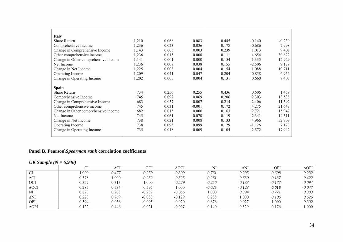
Italy Share Return 1,210 0.068 0.083 0.445 -0.140 -0.239 Comprehensive Income 1,236 0.023 0.036 0.178 -0.686 7.998 Change in Comprehensive Income 1,143 0.005 0.003 0.239 1.013 9.408 Other comprehensive income 1,236 0.015 0.000 0.111 4.654 30.622 Change in Other comprehensive income 1,141 -0.001 0.000 0.154 1.335 12.929 Net Income 1,236 0.008 0.038 0.155 -2.506 9.179 Change in Net Income 1,225 0.008 0.004 0.154 1.088 10.711 Operating Income 1,209 0.041 0.047 0.204 -0.858 6.956 Change in Operating Income 1,202 0.005 0.004 0.131 0.660 7.407 Spain Share Return 734 0.256 0.255 0.436 0.606 1.459 Comprehensive Income 745 0.092 0.069 0.206 2.303 13.538 Change in Comprehensive Income 683 0.037 0.007 0.214 2.406 11.592 Other comprehensive income 745 0.031 -0.001 0.172 4.275 21.643 Change in Other comprehensive income 682 0.015 0.000 0.163 2.721 15.947 Net Income 745 0.061 0.070 0.119 -2.341 14.511 Change in Net Income 738 0.021 0.008 0.133 4.966 52.909 Operating Income 738 0.095 0.099 0.129 -1.126 7.123 Change in Operating Income 735 0.018 0.009 0.104 2.572 17.942

Panel B. Pearson\Spearman rank correlation coefficients UK Sample (N = 6,946) CI ∆CI OCI ∆OCI NI ∆NI OPI ∆OPI CI 1.000 0.477 0.259 0.309 0.761 0.295 0.608 0.232∆CI 0.378 1.000 0.252 0.525 0.261 0.630 0.137 0.422OCI 0.357 0.313 1.000 0.529 -0.250 -0.133 -0.177 -0.094∆OCI 0.285 0.534 0.595 1.000 -0.025 -0.123 0.016 -0.047 NI 0.823 0.203 -0.237 -0.066 1.000 0.394 0.771 0.303∆NI 0.228 0.769 -0.083 -0.129 0.288 1.000 0.196 0.626OPI 0.302 0.594 0.036 -0.095 0.020 0.676 0.027 1.000∆OPI 0.122 0.446 -0.021 -0.007 0.140 0.529 0.176 1.000

34

35

∆OCI

German Sample (N = 4,121) CI ∆CI OCI NI ∆NI OPI ∆OPI CI 1.000 0.445 0.275 0.273 0.814 0.329 0.604 0.199∆CI 0.262 1.000 0.256 0.530 0.281 0.695 0.145 0.472OCI 0.342 0.256 1.000 0.503 -0.146 -0.023 -0.118 0.003 ∆OCI 0.275 0.489 0.511 1.000 0.020 -0.032 0.021 0.016NI 0.887 0.150 -0.131 0.039 1.000 0.375 0.726 0.214∆NI 0.143 0.868 0.002 -0.010 0.150 1.000 0.193 0.615OPI 0.517 -0.075 -0.182 0.039 0.635 -0.108 1.000 0.260 ∆OPI 0.030 0.548 0.025 0.012 0.019 0.621 0.039 1.000 French Sample (N = 3,586) CI ∆CI OCI ∆OCI NI ∆NI OPI ∆OPI CI 1.000 0.492 0.323 0.252 0.846 0.408 0.622 0.308∆CI 0.445 1.000 0.271 0.525 0.355 0.726 0.249 0.508OCI 0.397 0.319 1.000 0.529 -0.063 -0.017 -0.098 -0.021 ∆OCI 0.278 0.580 0.541 1.000 0.007 -0.015 0.004 -0.009NI 0.884 0.321 -0.078 0.027 1.000 0.463 0.741 0.347∆NI 0.344 0.807 -0.001 -0.013 0.374 1.000 0.322 0.677OPI 0.637 0.189 -0.071 0.040 0.728 0.203 1.000 0.405 ∆OPI 0.236 0.541 -0.006 0.017 0.253 0.652 0.343 1.000 Italian Sample (N = 1,094) CI ∆CI OCI ∆OCI NI ∆NI OPI ∆OPI CI 1.000 0.452 0.338 0.270 0.839 0.392 0.538 0.220∆CI 0.512 1.000 0.365 0.635 0.286 0.704 0.164 0.388OCI 0.511 0.477 1.000 0.504 -0.030 0.085 -0.063 -0.002 ∆OCI 0.376 0.765 0.635 1.000 0.032 0.099 0.033 0.042NI 0.762 0.228 -0.167 -0.047 1.000 0.422 0.647 0.263∆NI 0.383 0.716 0.049 0.098 0.403 1.000 0.253 0.567OPI 0.437 0.148 -0.090 0.014 0.569 0.213 1.000 0.344 ∆OPI 0.219 0.425 -0.001 0.104 0.251 0.544 0.407 1.000

Spanish Sample (N = 670) CI ∆CI OCI ∆OCI NI ∆NI OPI ∆OPI CI 1.000 0.566 0.588 0.388 0.722 0.391 0.512 0.287∆CI 0.546 1.000 0.425 0.727 0.353 0.564 0.251 0.358OCI 0.853 0.540 1.000 0.545 0.044 0.070 0.034 0.063∆OCI 0.515 0.855 0.610 1.000 0.057 0.034 0.037 0.042NI 0.575 0.197 0.063 0.028 1.000 0.512 0.672 0.336∆NI 0.239 0.577 0.078 0.069 0.335 1.000 0.353 0.569OPI 0.383 0.105 0.042 0.028 0.667 0.157 1.000 0.449 ∆OPI 0.200 0.291 0.035 0.022 0.327 0.523 0.429 1.000

Panel A exhibits univariate statistics for the models’ independent and dependent variables. Descriptive statistics are reported by countries. The samples comprise all firms listed on the London, Frankfurt, Paris, Milan and Madrid stock exchanges whose data necessary to the modelling process described previously are available under DATASTREAM for the financial period 1992-2004. Share return is the firm’s yearly raw share return calculated as the average of cumulated share return for 16, 17 and 18 months, from 12 months prior through 4, 5 and 6 months after the fiscal year end month (month 0). Return index, market value, net income and operating income have been obtained from DATASTREAM. Comprehensive income is computed as the yearly change in book value, i.e. ‘Ordinary Share Capital’ (DS Item #301) + ‘Reserves’ (Item #304) + ‘Preference Capital’ (DS Item #306), minored by ‘total equity issued’ (DS Item #406) and augmented by dividends paid (DS Item #434). All accounting variables are on a per share basis and are deflated by prior fiscal year end share price. Observations within the top and bottom 1% are excluded to avoid potential outliers’ issues. Panel B reports Pearson and Spearman rank correlation coefficients for the independent variables used in the analysis. The number of observations for every variable in each sample is equivalent to the one reported in Panel A. Pearson and Spearman correlation coefficients which are NOT significant at a 10% level are reported in bold characters. Consistent with Panel A, all the above accounting numbers are on a per share basis and are deflated by prior year end share price. CI Comprehensive income ∆CI Change in comprehensive income OCI Other comprehensive income ∆OCI Change in other comprehensive income NI Net income ∆NI Change in net income OPI Operating income ∆OPI Change in operating income

36

37

TABLE 3: Price Relevance of Operating Income

Table 3 exhibits the empirical results from the following OLS regression:

0 1 21 1

t tt t

t t

O IP OPIRET uP P

β β β− −

= + + + (6a)

Where RET

∆

t is the firm’s raw share return, OPIt is operating income per share and ∆OPIt is the change in operating income per share for each accounting period t. RETt is calculated here as the average of cumulated share return for 16, 17 and 18 months, from 12 months prior through 4, 5 and 6 months after the fiscal year end month (month 0). All variables except RETt are deflated by last financial period end firm’s cum-dividend share price Pt-1. Panel A presents the coefficients and t-statistics from conventional OLS regressions for each country sample. Following Abarbanell and Bushee (1998), we calculated the scale decile rank for each independent variable used in equation (6a) by ranking the values of the variables into ten portfolios (with ranks 0-9). The decile numbers obtained were then deflated by nine so that the constructed independent variable ranges on a positive unitary standardized interval. Panel B exhibits the coefficients an

LS regressions. d t-statistics obtained from ranking

els: *p<.1; **p<.05; ***p<.01.

a el A. Conventional OLS Mod

GE F

OThe following notations are used across pan P n el

UK RMANY RANCE ITALY SPAIN β0 0. 0. 0.0.01* -0.15*** 03*** 03*** 19*** (1.90) (-13.14) (3.48) (2.71) (9.69) β1 0.0.45*** 0.05*** 0.80*** 0.53*** 63*** (23.92) (6.87) (18.58) (8.41) (4.89) β2 0. 0. 0.20*** 0.40*** 49*** 0.31*** 49*** (7.81) (10.89 (8.48) (3.21) (3.06) ) N 7,915 4,900 4,123 1,198 733 Adj. R² 8.32% 3.30% 11.32% 8.70% 6.39% F-statistic 359.98*** 4.61*** 264.07*** 8.07*** 26.03*** 8 5

Panel B. Ranking OLS model

GE F SP UK RMANY RANCE ITALY AIN β0 -0.15*** -0.73*** -0.26*** -0.29*** -0.01 (-22.29) (-32.16) (-18.30) (-11.24) (-0.36) β1 00.27*** .71*** 0.45*** 0.46*** 0.36*** (26.38) (21.52) (19.80) (11.65) (6.53) β2 0. 010*** .46*** 0.28*** 0.24*** 0.17*** (9.68) (14.10 (12.34) (6.00) (3.09) ) N 7,915 4,900 4,123 1,198 733 Adj. R² 11.55% 14.82% 16.59% 16.62% 10.50% F-statistic 517.81*** 427.10*** 11.07*** 20.43*** 43.98*** 4 1

TABLE 4: Price Relevance of Net Income

Table 4 exhibits the empirical results from the following OLS regression:

0 1 21 1

t tt

t t

NI NItRET u

P Pβ β β

− −

∆= + + + (6b)

Where RETt is the firm’s raw share return, NIt is net income per share and ∆NIt is the change in net income per share for each accounting period t. RETt is calculated here as the average of cumulated share return for 16, 17 and 18 months, from 12 months prior through 4, 5 and 6 months after the fiscal year end month (month 0). All variables except RETt are deflated by last financial period end firm’s cum-dividend share price Pt-1. Panel A presents the coefficients and t-statistics from conventional OLS regressions for each country sample. Following Abarbanell and Bushee (1998), we calculated the scale decile rank for each independent variable used in equation (6b) by ranking the values of the variables into ten portfolios (with ranks 0-9). The decile numbers obtained were then deflated by nine so that the constructed independent variable ranges on a positive unitary standardized interval. Panel B exhibits the coefficients and t-statistics obtained from ranking OLS regressions. The following notations are used across panels: *p<.1; **p<.05; ***p<.01. Panel A. Conventional OLS Model

UK GERMANY FRANCE ITALY SPAIN β0 0.03*** -0.11*** 0.05*** 0.03*** 0.14*** (10.14) (-9.81) (6.54) (2.80) (7.70) β1 0.27*** 0.63*** 1.13*** 1.11*** 1.14*** (17.37) (17.58) (19.68) (12.35) (7.35) β2 0.03** 0.23*** 0.35*** 0.12 0.53*** (2.48) (8.65) (6.54) (1.34) (3.97) N 6,983 4,173 3,564 1,107 667 Adjusted R² 4.88% 9.17% 13.60% 14.80% 11.07% F-statistic 180.22*** 211.70*** 281.59*** 97.17*** 42.50***

Panel B. Ranking OLS model

UK GERMANY FRANCE ITALY SPAIN β0 -0.13*** -0.73*** -0.31*** -0.35*** -0.08*** (-18.54) (-34.45) (-22.05) (-14.79) (-2.67) β1 0.26*** 0.88*** 0.55*** 0.65*** 0.40*** (23.91) (26.36) (23.01) (16.88) (7.54) β2 0.06*** 0.37*** 0.27*** 0.15*** 0.21*** (5.08) (11.08) (11.28) (3.80) (4.06) N 6,983 4,173 3,564 1,107 667 Adj. R² 10.42% 22.01% 23.68% 27.78% 16.88% F-statistic 407.04*** 589.72*** 553.90*** 213.92*** 68.73***

38

0 1 21 1

t tt t

t t

CI CIRET uP P

β β β− −

∆= + + + (6c)

Where RETt is the firm’s raw share return, CIt is comprehensive income per share and ∆CIt is the change in comprehensive income per share for each accounting period t. RETt is calculated here as the average of cumulated share return for 16, 17 and 18 months, from 12 months prior through 4, 5 and 6 months after the fiscal year end month (month 0). All variables except RETt are deflated by last financial period end firm’s cum-dividend share price Pt-1. Panel A presents the coefficients and t-statistics from conventional OLS regressions for each country sample. Following Abarbanell and Bushee (1998), we calculated the scale decile rank for each independent variable used in equation (6c) by ranking the values of the variables into ten portfolios (with ranks 0-9). The decile numbers obtained were then deflated by nine so that the constructed independent variable

ts and t-statistics obtained from

els: *p<.1; **p<.05; ***p<.01.

a el A. Conventional OLS Model

GE FRANCE I

39

TABLE 5: Price Relevance of Comprehensive Income

Table 5 exhibits the empirical results from the following OLS regression:

ranges on a positive unitary standardized interval. Panel B exhibits the coefficienanking OLS regressions. r

The following notations are used across pan P n

UK RMANY TALY SPAIN β0 0.03*** -0.14*** 0.06*** 0.03** 0.19*** (9.92) (-13.00) (8.36) (2.46) (11.09) β1 00.20*** .38*** 0.70*** 0.71*** 0.38*** (14.19) (12.60) (14.66) (9.32) (4.40) β2 0. 0. 003*** 13*** .14*** 0.04 0.03 (3.09) (6.28) (3.76) (0.66) (0.32) N 7,186 4,643 3,865 1,138 677 Adj. R² 3.57% 4.99% 7.64% 9.56% 3.88% F-statistic 134.02*** 122.97*** 160.84*** 61.18*** 4.68*** 1

Pa el B. Ranking OLS model

GE F SPA

n

UK RMANY RANCE ITALY IN β0 -0.09*** -0.65*** -0.23*** -0.30*** 0.01 (-12.40) (-29.30) (-15.89) (-12.13) (0.43) β1 00.23*** .75*** 0.49*** 0.58*** 0.42*** (19.30 (7) (20.88) (19.43) (14.20) .15) β2 0.0.01 26*** 0.15*** 0.11*** 0.01 (0.58) (7.15) (6.08) (2.76) (0.18) N 7,186 4,643 3,865 1,138 677 Adj. R² 6.38% 13.55% 14.92% 20.75% 9.85% F-statistic 209.90*** 364.98*** 39.85*** 49.94*** 38.00*** 3 1

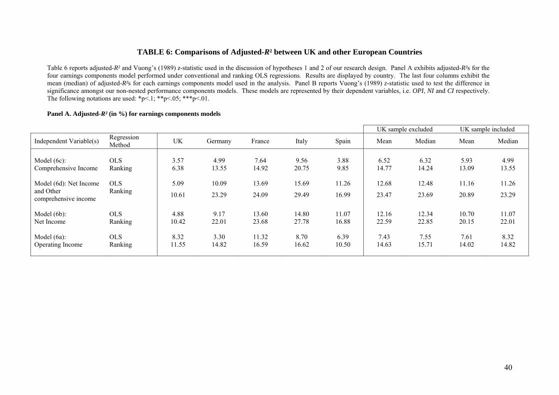
TABLE 6: Comparisons of Adjusted-R² between UK and other European Countries

Table 6 reports adjusted-R² and Vuong’s (1989) z-statistic used in the discussion of hypotheses 1 and 2 of our research design. Panel A exhibits adjusted-R²s for the four earnings components model performed under conventional and ranking OLS regressions. Results are displayed by country. The last four columns exhibit the mean (median) of adjusted-R²s for each earnings components model used in the analysis. Panel B reports Vuong’s (1989) z-statistic used to test the difference in significance amongst our non-nested performance components models. These models are represented by their dependent variables, i.e. OPI, NI and CI respectively. The following notations are used: *p<.1; **p<.05; ***p<.01. Panel A. Adjusted-R² (in %) for earnings components models

UK sample excluded UK sample included

Independent Variable(s) Regression Method UK Median Germany France Italy Spain Mean Median Mean

Model (6c): OLS 3.57 4.99 7.64 9.56 3.88 6.52 6.32 5.93 4.99Comprehensive Income Ranking 6.38 13.55 14.92 20.75 9.85 14.77 14.24 13.09 13.55 Model (6d): Net Income OLS 11 6 5.09 10.09 13.69 15.69 11.26 12.68 12.48 11.16 .2and Other comprehensive income

Ranking 10.61 23.29 24.09 29.49 16.99 23.47 23.69 20.89 23.29

Model (6b): OLS 4.88 9.17 13.60 14.80 11.07 12.16 12.34 10.70 11.07Net Income Ranking 10.42 22.01 23.68 27.78 16.88 22.59 22.85 20.15 22.01 Model (6a): 7.55 OLS 8.32 3.30 11.32 8.70 6.39 7.43 7.61 8.32Operating Income Ranking 11.55 14.82 16.59 16.62 10.50 14.63 15.71 14.02 14.82

40

41

TABLE 6 (continued)

Panel B: Vuong’s (1989) z-statistic for non-nested performance components models

UK Germany France Italy SpainNull-Hypothesis Ranking OLS Ranking OLS Ranking OLS Ranking OLS Ranking OLS NI > CI 48.00 144.88 31.86 Likelihood ratio 169.04 76.70 151.31 30.82 50.67 20.40 23.52 Variance ω² 0.03 0.05 0.03 22 0.10 0.13 0.06 0.11 0.10 0.13 0. z-statistic 3.30 ** 2.95*** * 7.61*** 2.69*** 7.47*** 5.43*** 7.52*** 3.00*** 4.35*** 1.69** 3 N 6,841 6,841 4,072 4,072 3,523 3,52 1,071 1,071 659 659 OPI > CI Likelihood ratio 156.97 192.54 -22.69 37.19 2.11 64.56 38.46 -7.08 -18.21 8.55 Variance ω² 0.10 16 0.27 0.10 0.16 0.18 0.12 0.18 0. 0.13 0.12 z-statistic -1.08 6.05*** 7.51*** -0.88 1.36* 3.10*** 1.54* -0.55 0.94 0.24 1 1,071 N 6,841 6,841 4,072 4,072 3,523 3,523 1,07 659 659 NI > OPI 12.14 Likelihood ratio -108.97 -47.67 54.55 131.84 112.86 37.90 68.88 11.84 21.41 Variance ω² 0.09 14 0.11 0.06 0.15 0. 0.15 0.18 0.23 0.19 0.11 z-statistic -4.30*** -2.31** 2.18** 5.57*** 0.63 4.96*** 2.75*** 4.41*** 1.07 2.46*** 1 N 6,841 6,841 4,072 4,072 3,523 3,523 1,071 1,07 659 659

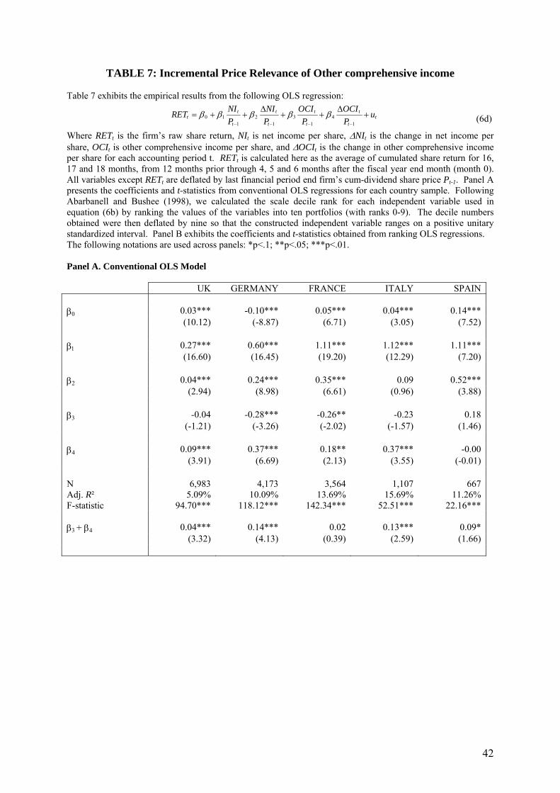
42

TABLE 7: Incremental Price Relevance of Other comprehensive income Table 7 exhibits the empirical results from the following OLS regression:

0 1 2 3 41 1 1 1

t t t tt t

t t t t

NI NI OCI OCIRET uP P P P

β β β β β− − − −

∆ ∆= + + + + + (6d)

Where RETt is the firm’s raw share return, NIt is net income per share, ∆NIt is the change in net income per share, OCIt is other comprehensive income per share, and ∆OCIt is the change in other comprehensive income per share for each accounting period t. RETt is calculated here as the average of cumulated share return for 16, 17 and 18 months, from 12 months prior through 4, 5 and 6 months after the fiscal year end month (month 0). All variables except RETt are deflated by last financial period end firm’s cum-dividend share price Pt-1. Panel A presents the coefficients and t-statistics from conventional OLS regressions for each country sample. Following Abarbanell and Bushee (1998), we calculated the scale decile rank for each independent variable used in equation (6b) by ranking the values of the variables into ten portfolios (with ranks 0-9). The decile numbers obtained were then deflated by nine so that the constructed independent variable ranges on a positive unitary standardized interval. Panel B exhibits the coefficients and t-statistics obtained from ranking OLS regressions.

FRANCE ITALY SPAIN

The following notations are used across panels: *p<.1; **p<.05; ***p<.01. Panel A. Conventional OLS Model UK GERMANY β0 0.03*** -0.10*** 0.05*** 0.04*** 0.14*** (10.12) (-8.87) (6.71) (3.05) (7.52) β1 12*** 1.11*** 0.27*** 0.60*** 1.11*** 1. (16.60) (16.45) (19.20) (12.29) (7.20) β2 0.04*** 0.24*** 0.35*** 0.09 0.52*** (2.94) (8.98) (6.61) (0.96) (3.88) β3 -0.04 -0.28*** -0.26** -0.23 0.18 (-1.21) (-3.26) (-2.02) (-1.57) (1.46) β4 0.09*** 0.37*** 0.18** 0.37*** -0.00 (3.91) (6.69) (2.13) (3.55) (-0.01) N 6,983 4,173 3,564 1,107 667 Adj. R² 5.09% 10.09% 13.69% 15.69% 11.26% F-statistic 94.70*** 118.12*** 142.34*** 52.51*** 22.16*** β3 + β4 0.04*** 0.14*** 0.02 0.13*** 0.09* (3.32) (4.13) (0.39) (2.59) (1.66)

TABLE 7 (continued) Panel B. Ranking OLS Model UK GERMANY FRANCE ITALY SPAIN β0 -0.76*** -0.13*** -0.33*** -0.38*** -0.11*** (-13.56) (-26.59) (-17.44) (-12.53) (-2.75) β1 0.25*** 0.83*** 0.54*** 0.65*** 0.40*** (22.37) (24.66) (22.69) (16.89) (7.56) β2 0.06*** 0.39*** 0.27*** 0.14*** 0.21*** (5.47) (11.85) (11.49) (3.61) (3.97) β3 -0.03*** -0.21*** -0.08*** -0.14*** 0.09* (-2.76) (-5.88) (-3.10) (-3.51) (1.68) β4 0.21*** 0.05*** 0.29*** 0.11*** -0.04 (4.08) (8.21) (4.53) (5.27) (-0.67) N 6,983 4,173 3,564 1,107 667 Adj. R² 10.61% 23.29% 24.09% 29.49% 16.99% F-statistic 208.26*** 317.71*** 283.77*** 116.77*** 35.14*** β3 + β4 0.02** 0.14*** 0.03 0.10*** 0.01 (2.15) (4.53) (1.25) (2.89) (0.16)

43

TABLE 8: Significance and Valuation-Sign of Other comprehensive incomes

Panel A. Statistical significance and signs of other comprehensive income variables

Panel A reports coefficients’ sign and statistical significance (p-value) of other comprehensive income (OCI) and change in other comprehensive income (∆OCI) obtained from model (6d) under conventional and ranking OLS regressions. Empirical results are exhibited by country sample. Coefficients in bold are not significant at a 10% level. Panel B exhibits the number of positive and negative signs for the OCI, ∆OCI and (OCI + ∆OCI) coefficients. These results are then split up taking into account whether the OLS coefficients are significant at a 1% level. Panel C presents the incremental value-relevance of other comprehensive income as measured by the absolute and relative difference in adjusted R² between models (6b) and (6d).

UK Germany France Italy Spain

OLS Ranking OLS Ranking OLS Ranking OLS Ranking OLS Ranking Other comprehensive income Sign <0 <0 <0 <0 <0 <0 <0 <0 >0 >0 (OCI) Significance

(p-value in %) 22.49 0.58 0.11 <.01 4.39 0.20 11.78 0.05 14.46 9.30

Change in OCI Sign >0 >0 >0 >0 >0 >0 >0 >0 <0 <0(∆OCI) Significance

(p-value in %) <.01 98.84 <.01 <.01 <.01 3.30 <.01 0.04 <.01 50.62

OCI + ∆OCI Sign >0 >0 >0 >0 >0 >0 >0 >0 >0 >0 Signi

(p-value in %) 0.09 <.01 <.01 ficance 3.18 69.52 21.06 0.96 0.40 9.80 87.01

44

TABLE 8 (continued) Panel B. Distribution of the OLS coefficients’ signs of other comprehensive income variables Positive signs Negative signs Significant Non-significant

at a 10% level at a 10% level Significant

at a 10% level Non-significant at a 10% level

Total

OCI - frequency 1 1 6 2 10* - in % 10% 10% 60% 20% 100% ∆OCI - frequency 0 0 2 10* 8 - in % 80% 0% 0% 20% 100% OCI + ∆OCI - frequency 7 3 0 0 10*- in % 70% 30% 0% 0% 100% * derived from multiplying five (countries) by two (different signs). Panel C. Incremental value-relevance of other comprehensive income variables

UK Germany France Italy Spain Mean(UK excluded)

Ranking OLS Ranking OLS Ranking OLS OLS Ranking OLS Ranking OLS Ranking

Absolute value 0.21 0.89 0.19 0.92 1.28 0.09 0.41 1.71 0.19 0.11 0.52 0.88Incremental

value-relevance ve value Relati 4.30 1.82 10.03 5.82 0.66 1.73 6.01 6.16 1.72 0.65 4.61 3.59

(Change in adj. R²)

45

TABLE 9: Number of early adopters of IFRS by country and by year over the period 1992-2004

Table 9 exhibits the number and percentage of early adopters using a breakdown by sampled country and by year over the pre-IAS-compliance period of analysis 1992-2004.

Germany France Italy SpainYear N N % N % % N %2004 381 60.9 52 8.2 23 8.7 8 7.82003 372 57.2 45 7.1 22 8.3 8 7.82002 361 54.1 41 6.5 21 7.9 8 7.82001 286 45.2 36 5.7 20 7.5 8 7.82000 257 40.9 31 4.9 20 7.5 8 7.81999 131 24.7 31 4.9 19 7.2 6 5.81998 81 15.9 30 4.7 16 6.0 5 4.91997 45 9.0 29 4.6 13 4.9 4 3.91996 2 4 9 20 4.2 22 3.5 11 4. 3.1995 13 2.7 19 3.0 10 3.8 3 2.91994 9 1.9 17 2.7 6 2.3 3 2.91993 8 1.7 12 1.9 6 2.3 3 2.91992 7 1.5 11 1.7 5 1.9 3 2.9

Total firm-year

observations 1,971 27.6% 376 4.58% 192 5.57% 71 5.30%

out of 7,130 out of 8,216 out of 3,445 out of 1,339

46

47

TABLE 10: Early Adopters Sensitivity Tests

In t Dt*It Dt*∆It It ∆ t Dt It Dt*∆OCIt OCIt ∆ t

Conventional OLS Model with CUMRET

Independent variable(s) N F-value Adj. R² tercep I *OC OCIGERMANY

- Operating Inc. (6a) 4,297 47.65*** 4.16%+ -0.08*** 0.06 0.02 0.15*** 0.37*** - Net Inc. (6b) 4,386 98.81*** 8.19%- -0.08*** -0.01 0.19*** 0.54*** 0.15*** - Comprehensive Inc. (6c) 4,052 72.83*** 6.62%+ -0.09*** -0.15** 0.15*** 0.44*** 0.08*** - Net Inc. and OCI (6d) 3,921 32.60*** 10.26%+ -0.08*** -0.05 0.20*** 0.62*** 0.15*** -0.53*** 0.36*** 0.05 0.10

FRANCE

- Operating Inc. (6a) 4,123 131.97*** 11.27%- 0.03*** 0.02 -0 1 .0 0.80*** 0.49*** - Net Inc. (6b) 3,898 149.54*** 13.23%+ 0.06*** -0.46* 0.03 1.10*** 0.34*** - Comprehensive Inc. (6c) 3,865 82.17*** 7.75%+ 0.06*** -0.56** 0.32* 0.73*** 0.14*** - Net Inc. and OCI (6d) 3,564 71.74*** 13.70%+ 0.05*** -0.49* 0.05 1.13*** 0.36*** -0.42 0.23 -0.23* 0.17*

ITALY

- Operating Inc. (6a) 1,198 29.30*** 8.63%- 0.03*** -0.07 0.41 0.53*** 0.29*** - Net Inc. (6b) 1,222 40.68*** 11.50%- 0.06*** 0.04 0.09 0.92*** 0.13 - Comprehensive Inc. (6c) 1,138 31.28*** 9.62%+ 0.03** 0.17 0.22 0.68*** 0.03 - Net Inc. and OCI (6d) 1,107 26.38*** 15.50%- 0.04*** 0.01 0.30 1.12*** 0.05 -0.27 0.06 -0.21 0.36***

SPAIN

- Operating Inc. (6a) 733 13.09*** 6.19%- 0.19*** -0.27 0.73 0.64*** 0.48*** - Net Inc. (6b) 738 17.44*** 8.18%- 0.19*** -0.49 1.31 0.92*** 0.40*** - Comprehensive Inc. (6c) 677 7.62*** 3.76%- 0.19*** -0.35 0.57 0.39*** 0.01 - Net Inc. and OCI (6d) 667 11.20*** 10.90%- 0.14*** -0.41 1.07 1.11*** 0.50*** -0.08 0.22 0.18 -0.01

The sign “+” (“-”) indicates greater (smaller) R-squared values in comparison with the models without early adopter interaction terms; The following notations are used: *p<.1; **p<.05; ***p<.01.

TABLE 11: Price Relevance of Operating Income

(results from non-early adopters) Table 11 exhibits the empirical results from the following OLS regression for the non-early adopters:

0 1 21 1

t tt t

t t

OPI OPIRET uP P

β β β− −

∆= + + + (6a)

Where RETt is the firm’s raw share return, OPIt is operating income per share and ∆OPIt is the change in operating income per share for each accounting period t. RETt is calculated here as the average of cumulated share return for 16, 17 and 18 months, from 12 months prior through 4, 5 and 6 months after the fiscal year end month (month 0). All variables except RETt are deflated by last financial period end firm’s cum-dividend share price Pt-1. Panel A presents the coefficients and t-statistics from conventional OLS regressions for each country sample. Following Abarbanell and Bushee (1998), we calculated the scale decile rank for each independent variable used in equation (6a) by ranking the values of the variables into ten portfolios (with ranks 0-9). The decile numbers obtained were then deflated by nine so that the constructed independent variable ranges on a

d t-statistics obtained from ranking

els: *p<.1; **p<.05; ***p<.01.

anel A. Conventional OLS Model

GERM FRANCE

positive unitary standardized interval. Panel B exhibits the coefficients anLS regressions. O

The following notations are used across pan P

ANY ITALY SPAIN β0 0 0.-0.01 .03*** 03*** 0.20*** (-0.71) (3.66) (2.64) (10.06) β1 0. 0.53*** 0.60*** 18*** 0.80*** (8.48) (18.09) (8.00) (4.55) β2 0. 0 0. 033*** .49*** 29*** .49*** (9.07) (8.33) (2.83) (3.01) N 2,846 3,826 1,084 674 Adj. R² 5.05% 11.56% 8.36% 6.28% F-statistic 76.75*** 251.14*** 50.45*** 23.56***

Panel B. Ranking OLS model

GER FRANCE SPA MANY ITALY IN β0 -0.27***-0.40*** -0.29*** -0.01 (-18.45) (-17.67) (-10.59) (-0.07) β1 0 00.52*** 0.45*** .46*** .33*** (16.60) (19.35) (11.07) (5.83) β2 0. 0. 025*** 0.28*** 23*** .19*** (8.13) (11.88 .61) (3.31) ) (5 N 2,846 3,826 1,084 674 Adj. R² 13.16% 16.84% 16.23% 10.08% F-statistic 216.71*** 388.48*** 105.99*** 38.79***

48

TABLE 12: Price Relevance of Net Income (results from non-early adopters)

Table 12 exhibits the empirical results from the following OLS regression for the non-early adopters:

0 1 21 1

t tt t

t t

NI NIRET uP P

β β β− −

∆= + + + (6b)

Where RETt is the firm’s raw share return, NIt is net income per share and ∆NIt is the change in net income per share for each accounting period t. RETt is calculated here as the average of cumulated share return for 16, 17 and 18 months, from 12 months prior through 4, 5 and 6 months after the fiscal year end month (month 0). All variables except RETt are deflated by last financial period end firm’s cum-dividend share price Pt-1. Panel A presents the coefficients and t-statistics from conventional OLS regressions for each country sample. Following Abarbanell and Bushee (1998), we calculated the scale decile rank for each independent variable used in equation (6b) by ranking the values of the variables into ten portfolios (with ranks 0-9). The decile numbers obtained were then deflated by nine so that the constructed independent variable ranges on a positive unitary standardized interval. Panel B exhibits the coefficients and t-statistics obtained from ranking OLS regressions.

The following notations are used across panels: *p<.1; **p<.05; ***p<.01.

N.B.: All early adopters have been dropped out from the sample Panel A. Conventional OLS Model

GERMANY FRANCE ITALY SPAIN β0 -0.03*** 0.05*** 0.03** 0.15*** (-3.16) (6.30) (2.43) (7.83) β1 0.62*** 1.15*** 1.12*** 1.11*** (16.03) (19.60) (11.70) (7.10) β2 0.13*** 0.35*** 0.09 0.51*** (4.40) (6.35) (0.91) (3.76) N 2,555 3,292 991 612 Adjusted R² 10.73% 14.21% 14.41% 11.03% F-statistic 154.58*** 273.60*** 84.42*** 38.93***

Panel B. Ranking OLS model

GERMANY FRANCE ITALY SPAIN β0 -0.46*** -0.32*** -0.35*** -0.07** (-22.40) (-21.79) (-14.36) (-2.14) β1 0.70*** 0.55*** 0.66*** 0.40*** (21.86) (22.47) (16.29) (7.07) β2 0.16*** 0.28*** 0.15*** 0.21*** (5.00) (11.38) (3.65) (3.70) N 2,555 3,292 991 612 Adj. R² 20.97% 24.60% 28.45% 16.22% F-statistic 339.94*** 538.10*** 198.01*** 60.23***

49

TABLE 13: Price Relevance of Comprehensive Income (results from non-early adopters)

Table 13 exhibits the empirical results from the following OLS regression for the non-early adopters:

0 1 21 1

t tt t

t t

CI CIRET uP P

β β β− −

∆= + + + (6c)

Where RETt is the firm’s raw share return, CIt is comprehensive income per share and ∆CIt is the change in comprehensive income per share for each accounting period t. RETt is calculated here as the average of cumulated share return for 16, 17 and 18 months, from 12 months prior through 4, 5 and 6 months after the fiscal year end month (month 0). All variables except RETt are deflated by last financial period end firm’s cum-dividend share price Pt-1. Panel A presents the coefficients and t-statistics from conventional OLS regressions for each country sample. Following Abarbanell and Bushee (1998), we calculated the scale decile rank for each independent variable used in equation (6c) by ranking the values of the variables into ten portfolios (with ranks 0-9). The decile numbers obtained were then deflated by nine so that the constructed independent variable

ficients and t-statistics obtained from

els: *p<.1; **p<.05; ***p<.01.

anel A. Conventional OLS Model

GER FRANCE ITA

ranges on a positive unitary standardized interval. Panel B exhibits the coefanking OLS regressions. r

The following notations are used across pan P

MANY LY SPAIN β0 -0.03*** 0 0.06*** .03** 0.20*** (-3.02) (8.13) (2.06) (10.94) β1 0. 00.44*** 0.73*** 69*** .38*** (13.20) (14.78) (8.48) (4.25) β2 0. 0.08*** 14*** 0.03 0.01 (3.24) (3.45) (0.44) (0.16) N 2,635 3,577 1,020 622 Adj. R² 7.83% 8.00% 8.88% 3.73% F-statistic 112.97*** 156.55*** 50.72*** 13.04***

Panel B. Ranking OLS model

GER FRANCE SPAIN MANY ITALY β0 --0.41*** 0.24*** -0.30** 0.02 (-19.49) (-15.70) (-11.53) (0.70) β1 0 00.64*** 0.50*** .57*** .42*** (18.39) (19.31) (13.26) (6.77) β2 0. 0 0.13*** .15*** 12*** 0.01 (3.73) (5.93) (2.75) (0.07) N 2,635 3,577 1,020 622 Adj. R² 16.12% 15.59% 20.41% 9.60% F-statistic 254.26*** 331.45*** 131.77*** 34.01***

50

TABLE 14: Incremental Price Relevance of Other comprehensive income

Table 14 exhibits the empirical results from the following OLS regression for the non-early adopters:

(results from non-early adopters)

0 1 2 3 41 1 1 1

t t t tt t

t t t t

NI NI OCI OCIRET uP P P P

β β β β β− − − −

∆ ∆= + + + + + (6d)

Where RETt is the firm’s raw share return, NIt is net income per share, ∆NIt is the change in net income per share, OCIt is other comprehensive income per share, and ∆OCIt is the change in other comprehensive income per share for each accounting period t. RETt is calculated here as the average of cumulated share return for 16, 17 and 18 months, from 12 months prior through 4, 5 and 6 months after the fiscal year end month (month 0). All variables except RETt are deflated by last financial period end firm’s cum-dividend share price Pt-1. Panel A presents the coefficients and t-statistics from conventional OLS regressions for each country sample. Following Abarbanell and Bushee (1998), we calculated the scale decile rank for each independent variable used in

ranks 0-9). The decile numbers ariable ranges on a positive unitary

tics obtained from ranking OLS regressions. *p<.01.

opped out from the sample

Panel A. Conventional OLS Mode

GERMAN F

equation (6b) by ranking the values of the variables into ten portfolios (withbtained were then deflated by nine so that the constructed independent vo

standardized interval. Panel B exhibits the coefficients and t-statishe following notations are used across panels: *p<.1; **p<.05; **T

N

.B.: All early adopters have been dr

l

Y RANCE ITALY SPAIN β0 -0.03*** 0.05*** 0.04*** 0.14*** (-3.05) (6.48) (2.70) (7.62) β1 120.62*** 1.13*** 1. *** 1.09*** (1(15.51) (19.14) 1.49) (6.96) β2 0.13*** 0.36*** 0.05 0.50*** (4.50) (6.41) (0.56) (3.68) β3 -0.01 -0.23* -0.20 0.18 (-0.07) (-1.75) (-1.37) (1.41) β4 0.13** 0 0.36 -0 .17** *** .01 (2.11) (1.96) (3.34) (-0.10) N 2,555 3,292 991 612 Adj. R² 1 14 11.0.86% .27% 15.31% 16% F-statistic 78 138. 4 20..84*** 04*** 5.77*** 23*** β3 + β4 0.08** 0.02 0.13*** 0.08 (2.15) (0.47) (2.58) (1.49)

51

Panel B. Ranking OLS Model

GERMANY FRANCE ITALY SPAIN β0 -0.50*** -0.34*** -0.38*** -0.10** (-17.86) (-17.03) (-12.03) (-2.35) β1 0.69*** 0.55*** 0.65*** 0.40*** (21.16) (22.16) (16.27) (7.11) β2 0.17*** 0.28*** 0.14*** 0.20*** (5.33) (11.56) (3.54) (3.63) β3 -0.05 -0.08*** -0.16*** 0.10 (-1.44) (-3.12) (-3.79) (1.63) β4 0.13*** 0.11*** 0.22*** -0.03 (3.70) (4.27) (5.28) (-0.59) N 2,555 3,292 991 612 Adj. R² 21.34% 25.00% 30.40% 16.32% F-statistic 174.27*** 275.29*** 109.22*** 30.85*** β3 + β4 0.10*** 0.02 0.09** 0.01 (3.43) (1.04) (2.44) (0.22)

Panel C. Incremental value-relevance of other comprehensive income variables

UK Germany France Italy Spain OLS Ranking OLS Ranking OLS Ranking OLS Ranking OLS Ranking

After excluding early adopters Absolute value* 0.21 0.19 0.13 0.37 0.06 0.40 0.90 1.95 0.13 0.10 Incremental

value-relevance Relative

value % 4.30 1.82 1.21 1.76 0.42 1.63 6.25 6.85 1.18 0.62

*Change in adj. R² Before excluding early adopters

Absolute value* 0.21 0.19 0.92 1.28 0.09 0.41 0.89 1.71 0.19 0.11 Incremental

value-relevance Relative

value % 4.30 1.82 10.03 5.82 0.66 1.73 6.01 6.16 1.72 0.65

*Change in adj. R²

52

9. REFERENCES

Abarbanell, J.S. and B.J. Bushee (1988). ‘Abnormal Returns to a Fundamental Analysis

Strategy’, The Accounting Review, January, 73(1), pp.19-45. Accounting Standards Board (1992). ‘Financial Reporting Standard N°3: Reporting Financial

Performance’, IAS Publications, October, London, UK.

Barker, R. (2004). ‘Reporting Financial Performance’, Accounting Horizons, 18(2), pp.157-

72.

Amir, E., T.S. Harris and E.K. Veuti (1993). ‘A Comparison of the Value-Relevance of US

vs. Non-US GAAP Accounting Measures Using Form 20-F Reconciliations, Journal of Accounting Research, 31, pp.230-64.

Association for Investment Management and Research (AIMR) (1993). ‘Financial Reporting

in the 1990’s and Beyond’, Charlottesville, Virginia: AIMR. Ball, R. (1995). ‘Making Accounting More International: Why, How, and How Far Will It

Go?’, Journal of Applied Corporate Finance, Fall, 8(3), pp.19-29. Barker, R. (2003). ‘Global Accounting Is Coming’, Harvard Business Review, April, pp.24-5.

Barth, M.E., W.H. Beaver and W.R. Landsman (2001). ‘The Relevance of the Value-Relevance Literature for Financial Accounting Standard Setting: Another View’, Journal of Accounting and Economics, 31, pp.77-104.

Beaver, W. (1981). ‘Financial Reporting: an Accounting Revolution’. Prentice-Hall

Contemporary, Englewood Cliffs, N.J.: Prentice-Hall. Biddle, G. and J.H. Choi (2006). ‘Is Comprehensive Income Useful?’, Journal of

Contemporary Accounting and Economics, 2(1), June, forthcoming. Black, F. (1980). ‘The Magic in Earnings: Economic Earnings vs. Accounting Earnings’,

Financial Analysts Journal, November-December, pp.19-24. Black, F. (1993). ‘Choosing Accounting Rules’, Accounting Horizons, 7, pp.1-17. Brief, R. P. and K.V. Peasnell (eds.) (1996). ‘Clean Surplus: a Link between Accounting and

Finance’, New York: Garland Publishing.

Brimble, M. and A. Hodgson (2004). ‘The Value Relevance of Comprehensive Income and Components for Industrial Firms’, Working Paper, Griffith University, Brisbane, Australia.

Bushman, R.M. and A.J. Smith (2001). ‘Financial Accounting Information and Corporate

Governance’, Journal of Accounting and Economics, 32, pp.237-333.

53

Cahan, S.F., S.M. Courtenay, P.L. Gronewoller and D.R. Upton (2000). ‘Value Relevance of Mandated Comprehensive Income Disclosure’, Journal of Business Finance and Accounting, 27 (9) & (10), November-December, pp.1273-301.

Chambers, D., T.J. Linsmeier, C. Shakespeare and T. Sougiannis (2005). ‘An Evaluation of

SFAS n°130 Comprehensive Income Disclosures’, Working Paper, University of Kentucky, Lexington.

Chartered Financial Analysts (CFA) Institute (2005). ‘A Comprehensive Business Reporting

Model: Financial Reporting for Investors’, October, Charlottesville, Virginia, 66p. Cheng, A., J. Cheung and V. Gopalakrishnan (1993). ‘On the Usefulness of Operating

Income, Net Income and Comprehensive Income in Explaining Security Returns’, Accounting and Business Research, 23, n°91, pp.195-203.

Cope, A.T., L.T. Johnson and C.L. Reither (1996). ‘The Call for Reporting Comprehensive

Income’, Financial Analysts Journal, March/April, 52(2), pp.7-12.

Easton, P. and G. Sommers (2003), ‘Scale and the Scale Effect in Market-based Accounting Research’, Journal of Business Finance & Accounting, January/March, 30(1) & 2, pp.25-55.

Fama, E. and J. McBeth (1973). ‘The Cross-Section of Expected Stock Returns’, Journal of

Finance, June, 47, pp.427-65.

Dhaliwal, D., K. Subramnayam and R. Trezevant (1999). ‘Is Comprehensive Income Superior

to Net Income as a Measure of Firm Performance?’, Journal of Accounting and Economics, 26, pp.43-67.

Easton, P. (1999), ‘Security Returns and Value Relevance of Accounting Data’, Accounting

Horizons, December, 3, pp.399-412. Easton, P. and T. Harris (1991), ‘Earnings as an Explanatory Variable for Returns’, Journal of

Accounting Research, Spring, pp.19-36.

Financial Accounting Standards Board (1997). ‘Statement of Financial Accounting Standard N°130: Reporting Comprehensive Income’, FASB, June 1997.

Foster, N. and N.L. Hall (1996). ‘Reporting Comprehensive Income: Shedding More Light on

Items Reported Directly in Equity’, CPA Journal, October, 66(10), pp.16-9. Harper, R., W. Meister and J. Strawser (1987). ‘The Impact of New Pension Disclosure Rules

on Perceptions of Debt’, Journal of Accounting Research, autumn, pp.327-30. Harper, R., W. Meister and J. Strawser (1991). ‘The Effect of Recognition Versus Disclosure

of Unfunded Postretirement Benefits on Lenders’ Perceptions of Debt’, Accounting Horizons, September, pp.50-6.

Harris, T. and J. Ohlson (1987). ‘Accounting Disclosures and the Market Valuation of Oil and

Gas Properties’, The Accounting Review, October, pp.651-70.

54

Hirst, E., and Hopkins, P. (1998). ‘Comprehensive income reporting and analysts’ valuation judgments’, Journal of Accounting Research, 36 (Supplement), pp.47-75.

Holthausen, R.W., and R.L. Watts (2001). ‘The Relevance of the Value-Relevance Literature

for Financial Accounting Standard Setting’, Journal of Accounting and Economics, 31, pp.3-75.

Kanagaretnam, K., R. Mathieu and M. Shehata (2005). ‘Usefulness of Comprehensive Income Reporting in Canada’, Working Paper, February, McMaster University, Ontario, Canada.

Leuz, C. and R.E. Verrecchia (2000). ‘The Economic Consequences of Increased Disclosure’, Journal of Accounting Research, 38 (Supplement), pp.91-124.

Linsmeier, T.J., Gribble, R., Jennings R.G., Lang, M.H., Penman, S.H., Petroni, K.R., Shores, D., Smith, J.H. and Warfield, T.D. (1997). ‘An Issues Paper on Comprehensive Income’, Accounting Horizons, June, 11(2), pp.120-6.

McDonald, E. (1997). ‘Heard on the Street: FASB Rule Will Offer Walk on Wild Side’, Wall

Street Journal, 30th of September, p.C1.

Ohlson, J.A. (1979). ‘Residual Analysis and the Private Value of Information’, Journal of

Accounting Research, autumn, pp.506-27.

International Accounting Standards Board (IASB) (2006). ‘Exposure Draft of Proposed

Amendments to IAS 1 Presentation of Financial Statements’, IASCF, March, 103p. Johnson, E. J., J.W. Payne and J.R. Bettman (1988). ‘Information Displays and Preference

Reversals’, Organizational Behavior and Human Decision Processes, 42, pp.1-21.

Kiger, J. E. and J.R. Williams (1977). ‘An Emerging Concept of Income Presentation’,

Accounting Historians Journal, 4 (2), pp.63-77. Kmenta, J. (1986). ‘Elements of Econometrics’, McMillan ed.

Leuz, C. and J. Wüstemann (2003). ‘The Role of Accounting in the German Financial System’ in Krahnen, J.P. and H. Reinhard (2003). ‘The German Financial System’, Chapter 14, Oxford University Press, London.

Lev, B. (1989). ‘On the Usefulness of Earnings and Earnings Research: Lessons and

Directions from Two Decades of Empirical Research’, Journal of Accounting Research, Supplement, pp.153-92.

Lin, S. (2006). ‘Testing the Information Set Perspective of UK Financial Reporting Standard

N°3: Reporting Financial Performance’, Journal of Business, Finance and Auditing, forthcoming.

O’Hanlon, J. and P. Pope (1999). ‘The Value Relevance of U.K. Dirty Surplus Accounting

Flows’, British Accounting Review, 31, 459-482.

55

Ohlson, J.A. (1989). ‘Accounting Earnings, Book Value, and Dividends: The Theory of the Clean Surplus Equation’, Unpublished Paper, Columbia University, USA.

Ohlson, J.A. (1991). ‘The Theory of Value and Earnings, and an Introduction to the Ball-

Brown Analysis’, Contemporary Accounting Research, 7, pp.1-19.

Roll, R. (1988). ‘R²’, Journal of Finance, July, pp.541-66.

Vuong, Q.H. (1989). ‘Likelihood Ratio Tests for Model Selection and Non-nested Hypotheses’, Econometrica, March, 57(2), pp.307-33.

White, G., A. Sondhi and D. Fried (1998). ‘The Analysis and Use of Financial Statements’,

2nd edition, New York, NY: John Wiley & Sons.

Ohlson, J.A. (1995). ‘Earnings, Book Values, and Dividends in Equity Valuation’,

Contemporary Accounting Research, 11(2), pp.661-78. Ohlson, J.A. (1999). ‘Earnings, Book Values, and Dividends in a Stewardship Setting with

Moral Hazard’, Contemporary Accounting Research, 16 (3), pp.525-40. Pope P.F. and P. Wang (2005). ‘Earnings Components, Accounting Bias and Equity

Valuation’, Review of Accounting Studies, 10, pp.387-407. Raedy, J. (2000). ‘A Reconciliation of Stock Market Anomalies’, Working paper, University

of North Carolina, Chapel Hill. Robinson, L.E. (1991). ‘The Time Has Come to Report Comprehensive Income’, Accounting

Horizons, 5(2), pp.107-12.

Sanbonmatsu, D., F. Kardes, S. Posvac and D. Houghton (1997). ‘Contextual Influences on

Judgement Based on Limited Information’, Organizational Behavior and Human Decision Processing, March, pp.251-64.

Skinner, D.J. (1999). ‘How Well Does Net Income Measure Firm Performance? A Discussion

of Two Studies’, Journal of Accounting and Economics, 26, pp.105-11.

Zeff, S.A. (1978). ‘The Rise of Economic Consequences’, The Journal of Accountancy,

December, pp.56-63.

56