Value of travel time reliability: A review of current evidence - Nexus

Transportation Research Part A 46 (2012) 720–741

Contents lists available at SciVerse ScienceDirect

Transportation Research Part A

journal homepage: www.elsevier .com/locate / t ra

Value of travel time reliability: A review of current evidence

Carlos Carrion ⇑, David LevinsonDepartment of Civil Engineering, University of Minnesota, 500 Pillsbury Drive SE, Minneapolis, MN 55455, USA

a r t i c l e i n f o

Article history:Received 25 February 2011Received in revised form 8 December 2011Accepted 5 January 2012

Keywords:VariabilityReliabilityTravel timeSchedulingMeta-analysis

0965-8564/$ - see front matter � 2012 Elsevier Ltddoi:10.1016/j.tra.2012.01.003

⇑ Corresponding author.E-mail addresses: [email protected] (C. CarrionURL: http://nexus.umn.edu (D. Levinson).

a b s t r a c t

Travel time reliability is a fundamental factor in travel behavior. It represents the temporaluncertainty experienced by travelers in their movement between any two nodes in a net-work. The importance of the time reliability depends on the penalties incurred by the trav-elers. In road networks, travelers consider the existence of a trip travel time uncertainty indifferent choice situations (departure time, route, mode, and others). In this paper, a sys-tematic review of the current state of research in travel time reliability, and more explicitlyin the value of travel time reliability is presented. Moreover, a meta-analysis is performedin order to determine the reasons behind the discrepancy among the reliability estimates.

� 2012 Elsevier Ltd. All rights reserved.

1. Introduction

Two of the most important values obtained from travel demand studies are the value of travel time (VOT), and the value oftravel time reliability (VOR). The former links the monetary values travelers (or consumers) place on reducing their traveltime (i.e. savings). The latter connects the monetary values travelers place on improving the predictability (i.e reducingthe variability) of their travel time.

The concept of value of travel time has a long established history through the formulation of time allocation models from aconsumer theory background. These models are reviewed thoroughly in Jara-Diaz (2007); a full chapter is dedicated to them.Also, the reader may refer to Small and Verhoef (2007) for a (succinct) review of the theory. In addition, more than a hundred ofempirical estimates of the value of travel time has been carried out by both researchers and practitioners. Reviews such asAbrantes and Wardman (2011), Shires and de Jong (2009), Wardman (1998, 2001, 2004), Zamparini and Reggiani (2007b,a)serve as compilations of VOT estimates, and summaries of what has become mainstream knowledge in the field of traveldemand. In contrast, the value of travel time reliability is a ‘‘newcomer’’ to this field, and although it has received increasedattention, the procedures for quantifying it are still a topic of debate. The differences among studies span almost every aspectsuch as: experimental design (e.g. presentation of reliability to the public in stated preference [SP] investigations); theoreticalframework (e.g. scheduling vs. centrality-dispersion); variability (unreliability) measures (e.g. interquartile range, standarddeviation; a requirement in the centrality-dispersion framework); setting (or estimating) the preferred arrival time (e.g. assum-ing work start time as preferred arrival time in the scheduling approach); data source (e.g. revealed preference [RP] vs. statepreference [SP]); and others. As a consequence, value of reliability estimates also exhibit a significant variation across studies.

In this paper, a systematic review of the theoretical and empirical research on travel time reliability is presented. Firstly,the concept of travel time reliability is discussed as it has become ‘‘defined’’ in the literature. Secondly, the most commontheoretical models (scheduling and mean-variance [centrality-dispersion]) are described; others (e.g. mean-lateness) are

. All rights reserved.

), [email protected] (D. Levinson).

http://dx.doi.org/10.1016/j.tra.2012.01.003

mailto:[email protected]

mailto:[email protected]

http://nexus.umn.edu

http://dx.doi.org/10.1016/j.tra.2012.01.003

http://www.sciencedirect.com/science/journal/09658564

http://www.elsevier.com/locate/tra

C. Carrion, D. Levinson / Transportation Research Part A 46 (2012) 720–741 721

also briefly covered. Thirdly, the empirical evidence is compiled, and surveyed; the similarities and discrepancies of resultsacross studies are discussed. Fourthly, a meta-analysis is performed to identify the sources of variations in travel time reli-ability estimates, and to provide an even more objective comparison of the reasons behind the estimates variability acrossstudies. Lastly, the article is concluded.

2. Travel time reliability: concepts

The concept of travel time can be defined as the time elapsed when a traveler displaces between two (distinct) spatialpositions. Certainly, this definition is applicable to any transportation mode (or combinations of them) regardless of theinherent differences across them. This is expected as travel time is typically understood as a one dimensional quantity (var-iable). Furthermore, travel time can be divided into several components depending on the analyst. For example, travel timeof public transit modes tends to be split into waiting time, in-vehicle time, transfer time, and others.

In road networks, travel time may be split into two components: free flow time, and additional time. The former refers tothe amount of time it takes a driver to arrive at his/hers destination without encountering any (or very little) traffic. The lat-ter refers to each increase of travel time due to variations in the traffic conditions. These variations may be predictable (e.g.peak-hour congestion), or unpredictable (e.g. vehicular crashes).

The predictable variations are events (i.e. traffic congestion) expected by travelers, and thus travelers (in principle) per-form the necessary adjustments to offset the added costs (e.g. departing earlier to avoid arriving late at work). Such events(i.e. traffic congestion) are by itself a topic of interest to many researchers focusing on traffic flow theory (see Daganzo (2007)for an introduction to traffic flow theory). In transportation research, the morning peak-hour congestion is considered as aclassic problem of trip scheduling under deterministic traffic conditions. Vickrey (1969) presented a solution to the problemwith a single deterministic bottleneck model between an origin and destination, fixed and homogeneous travel demand, andendogenous departure time (i.e. trip scheduling choices). This model was further extended by Arnott et al. (1990), Laih(1994), Arnott et al. (1993), Arnott et al. (1994), Garcia (1999), Newell (1987), Daganzo and Garcia (2000), Daganzo(1985), Daganzo (1995) and others. The interested reader on bottleneck theory, and its pricing applications may consult Yangand Huang (2005) and Small and Verhoef (2007).

The unpredictable variations are directly linked to the uncertainty of travel time. This uncertainty has been divided inthree elements by Wong and Sussman (1973): variation between seasons and days of the week; variation by changes in tra-vel conditions because of weather and crashes or incidents; and variations attributed to each traveler’s perception. Nicholsonand Du (1997) lists also the components of uncertainty as variations in the link flows and variations in the capacity. There-fore, the unpredictable variations trace their source at both the demand side (e.g. traveler’s heterogeneous behavior) andsupply side (e.g. traffic signal failure) of a transportation system.

Travel time reliability is closely linked to the unpredictable variations. This suggests that travelers choose under an uncer-tain environment as they may fail to predict their exact travel time before scheduling their trips (i.e. choosing a departuretime). In the case of predictable variations, the travelers may adjust their departure time choice, and still be certain of arriv-ing on time at their destinations. This is true even in a transportation system with high congestion. Notice that travelers arechoosing under a certain environment. Therefore, it’ll be incorrect to consider predictable variations as examples of traveltime (un) reliabiility (Bates et al., 2001). It should be noted that this travel time uncertainty may also extend to other choicedimensions (e.g. mode, route). Furthermore, the concept of travel time (un)reliability is defined as interchangeable with tra-vel time variability (or unpredictable variation) in the transportation research literature; high variability means high unre-liability, and vice versa. Consequently, it is natural to think of travel time in two dimensions: frequency, and magnitude. Inother words, travel time defined as a distribution in the probability theory sense. In this way, travel time (un)reliability canbe associated as a measure of spread to the travel time distribution. Distinct approaches have been proposed to model traveltime reliability, and they are reviewed in the subsequent section. Moreover, similarities (i.e. travel time composed of deter-ministic and random elements) may be drawn to other transportation modes despite the fact that the concepts were mostlyexplained with a focus on road transportation.

3. Theoretical frameworks

3.1. Centrality-dispersion

The approach is mostly known in the context of risk-return models in finance. A decision-maker looks to maximize theoption’s return while minimizing its associated risk. The option’s return is represented by the expected value, and the risk bythe variance (see Markowitz (1999) for an overview). In a transportation context, the framework is based on the notion thatnot only travel time is a source of disutility, but also travel time variability (or unreliability). Thus, the formulation (with alinear-additive form) of the model, in a consumer theory background, is as follows:

U ¼ c1lT þ c2rT ð1Þ

The traveler is minimizing the sum of the two terms (objective function for an unspecified choice dimension): the‘‘expected’’ travel time of the trip, and the travel time variability of the trip. The ‘‘expected’’ travel time (lT) is included

722 C. Carrion, D. Levinson / Transportation Research Part A 46 (2012) 720–741

as a centrality measure (e.g. mean) of the travel time distribution. The travel time variability (rT) is included as dispersionmeasure (e.g. standard deviation) of the travel time distribution. The c coefficients are exogenous parameters. Typically, thechoice dimension is route choice, and the centrality (dispersion) measure is mean (variance or standard deviation) amongstudies using this approach. Mean-variance is also usual name the approach is known in the transportation literature,despite the fact that the centrality and dispersion measures vary among studies.

In the transportation literature, the framework was introduced by Jackson and Jucker (1982). Their original formulation is:

Minimize EðTpÞ þ kkVarðTpÞp 2 PAB

kk > 0 ð2Þ

A traveler k has a priori information of the mean (E(Tp)), and variance (Var(Tp)) of the travel time distribution for eachroute in their choice set (P) between an origin-destination pair (AB). kk indicates the degree of risk aversion of the travelerk. The choice dimension is the route. Succinctly, a traveler k, with a degree of risk aversion kk, chooses the route that min-imizes the objective function Eq. (2) given the expected and variance of the travel time distribution. The model proposed byJackson and Jucker (1982) is usually estimated using discrete choice methods with the linear-additive specification given inEq. (1). In this utility form plus a travel cost variable (c3C), marginals rate of substitution may be computed to obtain impor-tant quantities such as the value of travel time (VOT), value of travel time reliability (VOR), and the reliability ratio (RR).These are defined formally in the previous order as,

VOT ¼ @U=@lT

@U=@Cð3Þ

VOR ¼ @U=@rT

@U=@Cð4Þ

RR ¼ @U=@rT

@U=@lT¼ VOR

VOTð5Þ

In essence, this framework is based on expected utility theory developed by Von Neuman and Morgenstern (1944). Thetheory prescribes a set of axioms about how decision-makers deal with risky prospects (set of alternatives where a choiceis selected) based on distinct states of nature (or states of the world). In simple words, there are several alternatives withseveral possible states of natures (the distribution of outcomes for each alternative), and associated to each combinationof alternative and state of nature there is an outcome. In the transportation context, the set of alternatives could be routes,modes, schedules. The states of nature could be traffic signal failure, crashes, and others. The outcomes are likely to be thedistribution of travel times for each alternative. In addition, the decision-maker ranks the risky prospects through theassumption of the existence of an ordinal utility function (i.e. U = f(outcome); the utility function associates a single realnumber to each outcome), and prefers the alternative with the highest expected utility (E(U)). Furthermore, an importantfeature of the expected utility framework is based on decision-making under risk. In other words, there’s a different betweenrisk, where probabilities are known or at least knowable, and uncertainty, where probabilities are unknown. This differencemay not be particularly useful for most practical purposes, or it may be irrelevant by considering subjective probability, andthe axiomatic approach of expected utility theory (Takayama (1993) Chapter 5). Readers may also refer to Mas-Colell et al.(1995)Varian (1978), for treatments of expected utility theory.

The functional form of the utility function is not restricted by the axioms. In fact, the functional form chosen should bebased on its close description of a decision-maker’s behavior. The functional form determines the risk preferences of the deci-sion-maker. Functional forms may be selected based on regression analysis of experiments (e.g. gambling games that provideobservations revealing the utility function) or computationally convenient forms (Hazell and Norton (1986) Chapter 5).

In the transportation literature, several functional forms have been considered to understand the risk behavior of travel-ers. Polak (1987) considered an alternative formulation to Jackson and Jucker (1982), where he defined the utility function ofthe traveler as a polynomial of second degree with respect to the travel time variable (T). Formally,

U ¼ c1T þ c2T2 ð6Þ

This functional form Eq. (6) is known in the microeconomics literature (see Varian, 1978, Chapter 11, pp. 189) as equiv-alent to the mean-variance model under expected utility theory. This can be seen by applying the expectation operator to Eq.(6), and using a simple identity (Var(X) � E(X2) � (E(X))2),

EðUÞ ¼ c1EðTÞ þ c2ðEðTÞÞ2 þ c2VarðTÞ ð7Þ

An important consideration is that the omission of the additional term [(E(T))2] in Eq. (7) might bias the estimates of c2,especially when the formulation in Eq. (6) is accurate. In addition, the c2 indicates whether the traveler prefers alternatives(e.g. routes) with high variance of travel time (risk prone), low variance of travel time (risk averse) or only cares about theexpected travel time (risk neutral). Furthermore, higher degrees of polynomials may be specified, and consequently in ex-pected utility forms will lead to higher moments to be included. Another formulation proposed by Polak (1987) is


U ¼ �ec1T ð8Þ

This functional form Eq. (8) is also known in the microeconomics literature (see Varian, 1978, Chapter 11, pp. 189–190); itdescribes a traveler with absolute risk aversion.

Senna (1994) introduced a more general form based on the previous mentioned work, where the utility function is givenby a algebraic term of degree b.

U ¼ c1Tb ð9Þ

The utility function can be written in terms of expected utility, by applying the expectation operator, and by consideringsome simple identities such as the definition of covariance, in the following form:

EðUÞ ¼ c1 E Tb2

� �� 2þ c1Var T

b2

� �ð10Þ

The Eq. (10) exhibits certain properties. The b parameter estimates the degree of risk aversion/proneness by the travelers.Another important property is that the value of time and the value of variability (reliability) depend directly on the traveltime distribution. The reader should refer to appendix 2 in Senna (1994) for the mathematical proofs.

It should be noted that all the previous c coefficients are parameters to be estimated, and expected to be negative.

3.2. Scheduling delays

Historically, this approach has been linked to the departure time choice (or trip scheduling) studies. The basis for the ap-proach rests on the time constraints (e.g. work start time) a traveler may face, and thus it associated costs due to early or latearrival. This leads to the idea of a traveler intrinsic choice of a preferred arrival time (PAT); the point of reference that delim-its whether an arrival is early or late. Gaver (1968) is one of its earliest proponents. He introduced a theoretical frameworkfor describing variability in trip-scheduling decisions. He considered distinct head start strategies for given delay distribu-tions along with the costs of arriving early or late. In addition, statistical estimation procedures (non-parametric and para-metric) are provided to estimate the probability density distribution of the trip delay, when it is unknown to the researcher.Vickrey (1969), as described previously, also considered the trade off travelers face between queue delay, and schedule delayof arriving early or late at work. Furthermore, a similar hypothesis is the existence of a ‘‘safety margin’’ advocated by Knight(1974) and Pells (1987). Knight (1974) suggested that travelers consider a slack time (i.e. safety margin) between their (aver-age) arrival time and their work start time. This safety margin allows the reduction of the probability of late arrivals, andimplies that travelers have a preference of arriving early to work (i.e. existence of positive utility for the time spent at workbefore work start time). In essence, Knight (1974) hypothesizes that the departure time chosen happens when the marginalutility of time spent at home is equal to the marginal utility of arriving early to work plus the marginal utility of arriving lateto work. Pells (1987) further argued that two opposite existing factors are at play: the need to minimize the frequency of latearrivals, and maximize the time spent at home relative to the early time spent at work. Travelers meet the first factor byallocating a safety margin, and they meet the second factor by maintaining the safety margin at required levels (i.e. safetymargins are acceptable when there’s more time spent at home relative to early time spent at work).

Another important contribution is by Small (1982), based on some of the previous articles (mostly Gaver (1968) andVickrey (1969)). He formulates a theoretical model based on the traditional utility maximization framework (i.e. consumerbehavior; see (Varian, 1978)) with insights from time allocation models (e.g. Becker (1965), DeSerpa (1971), Bruzelius(1979)). Small (1982)’s model consists of tying explicitly the departure time choice, and also adding a workplace constraint(i.e. an equation linking departure time, and working hours with merits or penalties to the wage rate; workplace policieswhere pay is docked by tardiness or bonuses are given for arrival on time) to the utility function of a traveler. In thisway, the traveler’s utility is influenced by the departure time, and also the value of time is influenced by the workplace con-straint. Properties of this formulation may be reviewed in Jara-Diaz (2007, Chapter 2, pp. 67–69), and Carrion (2010, Chapter2, pp. 11–15). Furthermore, he specifies a functional form for the (indirect) utility of scheduling:

Uðtd; PATÞ ¼ c1T þ c2SDEþ c3SDLþ c4DL ð11Þ

This is a linear-additive form, where the c coefficients are parameters to be estimated, and expected to be negative. In thisequation, the travel time (T) is not only included but also the scheduling delays which are divided by early (SDE; defined asMax(0,PAT � [T + td])) and late (SDL; defined as Max(0, [T + td]) � PAT) arrivals according to a preferred arrival time (PAT), anda binary term DL to indicate whether it is a late arrival or not (SDL > 0). The SDE, SDL and DL terms represent schedulingconsiderations for the workplace constraint. td is the decision variable (usually a continuous real variable for mathematicalmodels), and it represents the traveler’s departure time choice. Up until this point, the scheduling delay framework describestravelers’ choices under certainty. Moreover, Bates et al. (2001) points out that capacity restrictions (i.e. td is no longer inde-pendent of T; travelers cannot choose the same td as queueing is now present) of the transportation facility readily translatesthis framework to one extensively studied using bottleneck models (e.g. Arnott et al. (1990), Laih (1994), Arnott et al. (1993),Arnott et al. (1994)). This implies (as discussed in Section 2) the decomposition of travel time into: free flow travel time, andadditional travel time due to recurrent congestion.


The model proposed by Small (1982) is usually estimated using discrete choice methods (i.e. the departure times are dis-crete intervals if scheduling is the choice situation) with the linear-additive specification given in Eq. (11). In this utility formplus a travel cost variable (c5C), marginals rate of substitution may be computed to obtain important quantities such as thevalue of travel time (VOT), value of scheduling delay early (VSDE), and the value of scheduling delay late (VSDL). Researchersoften discard the lateness penalty variable (DL), because it adds a discontinuity that is inconvenient to mathematical opti-mization models (gradient-based), and a missing lateness penalty may translate into a higher lateness scheduling delay ineconometric models. These are defined formally in the previous order as,

VOT ¼ @U=@T@U=@C

ð12Þ

VSDE ¼ @U=@SDE@U=@C

ð13Þ

VSDL ¼ @U=@SDL@U=@C

ð14Þ

3.2.1. Scheduling delays + dispersionIn Noland and Small (1995), the previous scheduling approach is extended to include explicitly the uncertainty of travel

time (i.e. unpredictable variation; see Section 2). This uncertainty is expressed in the form of a random variable (Tr; preserv-ing Noland and Small (1995) notation) with a given probability density function, and with the restriction of being greater orequal to zero.

EðUðtdÞÞ ¼Z 1

0UðtdÞf ðTrÞdTr ¼ c1EðTÞ þ c2EðSDEÞ þ c3EðSDLÞ þ c4PL ð15Þ

The objective function of the traveler changes (also the utility function is traded for a trip cost form in Noland and Small(1995), but we choose to keep it for coherency), and now the consumer maximizes the expected utility E(U(td)) by choosingthe optimal td (see Eq. (15)) for a given probability density function of Tr. The elements of Eq. (15) include the schedulingcosts for early (SDE) vs. late (SDL) arrival at work presented earlier (see Eq. (11)), but also the last term employs the distri-bution of the random variable (Tr) in order to compute the probability of being late. PL is simply E(DL) (note DL is an indicatorfunction) conditional on td. Therefore, the last term PL also contains the costs of travel time unreliability as the dispersion (orvariability) of the travel time distribution affects the calculated probabilities. In addition, travel time dispersion (or variabil-ity) may increase the propensity of early arrivals, and thus high earliness costs can be incurred. This implies variability andscheduling costs are related. In fact, Bates et al. (2001) argues that c2 E(SDE) + c3E(SDL) may approximate the c02 rT in thecentrality-dispersion model (see Section 3.1) under certain conditions: travel time distribution is independent of departuretime; c4 = 0 in Eq. (15) or no lateness penalty; departure time is continuous; congestion dynamics are neglected as in traveltime is independent of departure time. Such mathematical properties and others are discussed in detail in Bates et al. (2001).

Recent work by Fosgereau and Karlstrom (2010) proved mathematically the previous statement by Bates et al. (2001)(scheduling models approximated by mean-variance models). They indicate this can be achieved with knowledge not onlyof the estimated parameters (c1 and c2 in Eq. (1)) for the expected travel time and variance, but also the travel time distribu-tion, and the optimal probability of being late. This proof follows the assumptions presented earlier by Bates et al. (2001), andalso the obvious assumptions the mean of random variable (Tr; they actually use a standardized form with mean 0 and var-iance 1) is defined (i.e exists), and that it has an invertible distribution. These assumptions are more general than the previousones of assuming the density function of the random variable (Tr) follows an uniform or exponential distribution (see Bates etal., 2001; Polak, 1996; Noland and Small, 1995; Small and Verhoef, 2007). The interested reader should refer directly to Fos-gereau and Karlstrom (2010), especially appendix A for more details. An empirical verification is also included in the paper.

It should be noted that all the previous c coefficients are parameters to be estimated, and expected to be negative.Other recent work has followed different paths: inclusion of risk attitudes in scheduling models (Senbil and Kitamura,

2004; Michea and Polak, 2006; Schwanen and Ettema, 2009; Li et al., 2010); alternative formulation of schedule early(SDE), and schedule late (SDL) (Tilahun and Levinson, 2010); and scheduling preferences with non-constant marginal util-ities or time-varying parameters (Tseng and Verhoef (2008) and Fosgereau and Engelson (2011) and Jenelius et al. (2011)).

In Li et al. (2010), a non-linear utility specification (they assume a utility function of the form U ¼ c1x1�a

1�a, where x is anyvariable in the model and a represents risk attitude) is used like in the other mentioned studies (e.g. Michea and Polak(2006)), but the parameter indicating risk attitude (a) was assumed random, and thus the parameters of its population den-sity function can be estimated using a mixed logit formulation. The idea of risk attitudes has been considered before inmicroeconomics, and discussed implicitly in Section 3.1.

Tilahun and Levinson (2010) introduces a new approach for measuring SDE and SDL in Eq. (11) consisting of two mo-ments: the first representing on average how early the traveler has arrived by using that route; and the second representingon average how late that individual arrived by using that particular route. They assume that the deviation of the two mo-ments (average late or average early) from the most frequent experience is a representative way of getting together the pos-sible range and frequencies experienced by the travelers. Thus, this measure may considers scheduling constraints as well,albeit not separately from (un)reliability of travel time.


The scheduling preferences models (Tseng and Verhoef (2008) and Fosgereau and Engelson (2011) and Jenelius et al.(2011)) generalize Small (1982) by assuming the c parameters (except for the binary lateness penalty, which is discarded)in Eq. (11) are time-dependent (earliness and lateness penalties vary by time of day). Tseng and Verhoef (2008) introducedthe formulation based on Vickrey (1973). Fosgereau and Engelson (2011) extended the formulation to account for randomtravel times. Jenelius et al. (2011) considered chained trips, and thus more than one activity. In addition, Jenelius (2011) ex-tends his previous chained trip formulation to consider random travel times.

3.3. Mean-lateness

This approach is widely used in passenger rail in the UK, and it was proposed by the Association of Train Operating Com-panies (ATOC, n.d.). It consists of two elements under the expected utility paradigm: schedule journey time (Sched), and themean lateness at destination (L). The former refers to the travel time between the actual departure time and the scheduledarrival time, and the latter refers to the mean of the lateness. The lateness is defined as the time between scheduled depar-ture and actual departure (lateness at boarding), and time between scheduled arrival and actual arrival (lateness at destina-tion). In the original ATOC formulation (see Eq. 16) only the mean (positive [L+]; negative values meaning early arrivals arenot considered) lateness at destination is considered, but this is expanded (see Eq. (17)) in Batley and Ibanez (2009) to in-clude the lateness at boarding (positive [B+]; negative values meaning early departures are not considered) as well, plus thetrain fare is added to calculate marginal rates of substitution between temporal quantities and travel cost (e.g. value of time[VOT]). It should be noted that Batley and Ibanez (2009) also tested the inclusion of another variable (c5rT) representing thestandard deviation of the in-vehicle journey time.

EðUÞ ¼ c1SchedT þ c2Lþ ð16ÞEðUÞ ¼ c1SchedT þ c2Lþ þ c3Bþ þ c4C ð17Þ

It should be noted that all the previous c coefficients are parameters to be estimated, and expected to be negative.

4. Empirical evidence

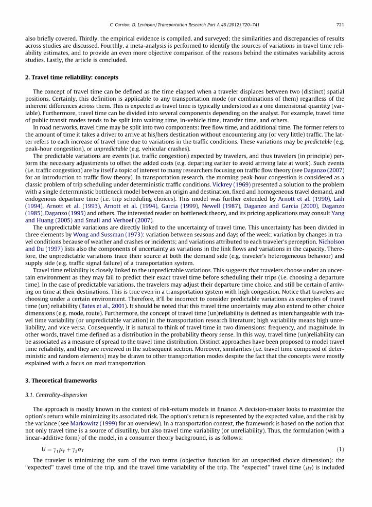
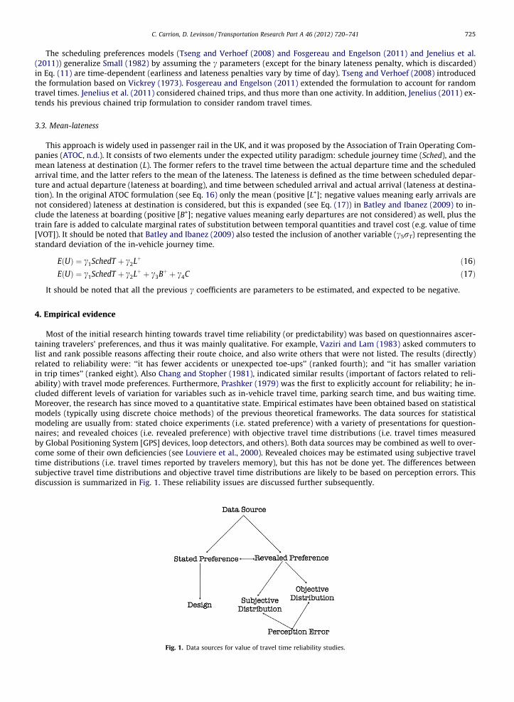
Most of the initial research hinting towards travel time reliability (or predictability) was based on questionnaires ascer-taining travelers’ preferences, and thus it was mainly qualitative. For example, Vaziri and Lam (1983) asked commuters tolist and rank possible reasons affecting their route choice, and also write others that were not listed. The results (directly)related to reliability were: ‘‘it has fewer accidents or unexpected toe-ups’’ (ranked fourth); and ‘‘it has smaller variationin trip times’’ (ranked eight). Also Chang and Stopher (1981), indicated similar results (important of factors related to reli-ability) with travel mode preferences. Furthermore, Prashker (1979) was the first to explicitly account for reliability; he in-cluded different levels of variation for variables such as in-vehicle travel time, parking search time, and bus waiting time.Moreover, the research has since moved to a quantitative state. Empirical estimates have been obtained based on statisticalmodels (typically using discrete choice methods) of the previous theoretical frameworks. The data sources for statisticalmodeling are usually from: stated choice experiments (i.e. stated preference) with a variety of presentations for question-naires; and revealed choices (i.e. revealed preference) with objective travel time distributions (i.e. travel times measuredby Global Positioning System [GPS] devices, loop detectors, and others). Both data sources may be combined as well to over-come some of their own deficiencies (see Louviere et al., 2000). Revealed choices may be estimated using subjective traveltime distributions (i.e. travel times reported by travelers memory), but this has not be done yet. The differences betweensubjective travel time distributions and objective travel time distributions are likely to be based on perception errors. Thisdiscussion is summarized in Fig. 1. These reliability issues are discussed further subsequently.

Fig. 1. Data sources for value of travel time reliability studies.


4.1. Stated preference studies

Most of the estimates of valuation of reliability have been obtained through stated choice experiments. In fact, Bates et al.(2001) argued that (at the time of publication) there were no adequate real examples at the level of detail required for ascer-taining reliability estimates using revealed preference data (RP). Thus, they considered stated preference as the best bet,which had dominated completely the empirical studies (and its estimates) so far. However, they admitted that survey design(i.e. presentation of questions) may affect the outcome of the reliability estimates. This is likely as travel time reliability isdifficult to present to subjects without any statistical background unlike travel time savings.

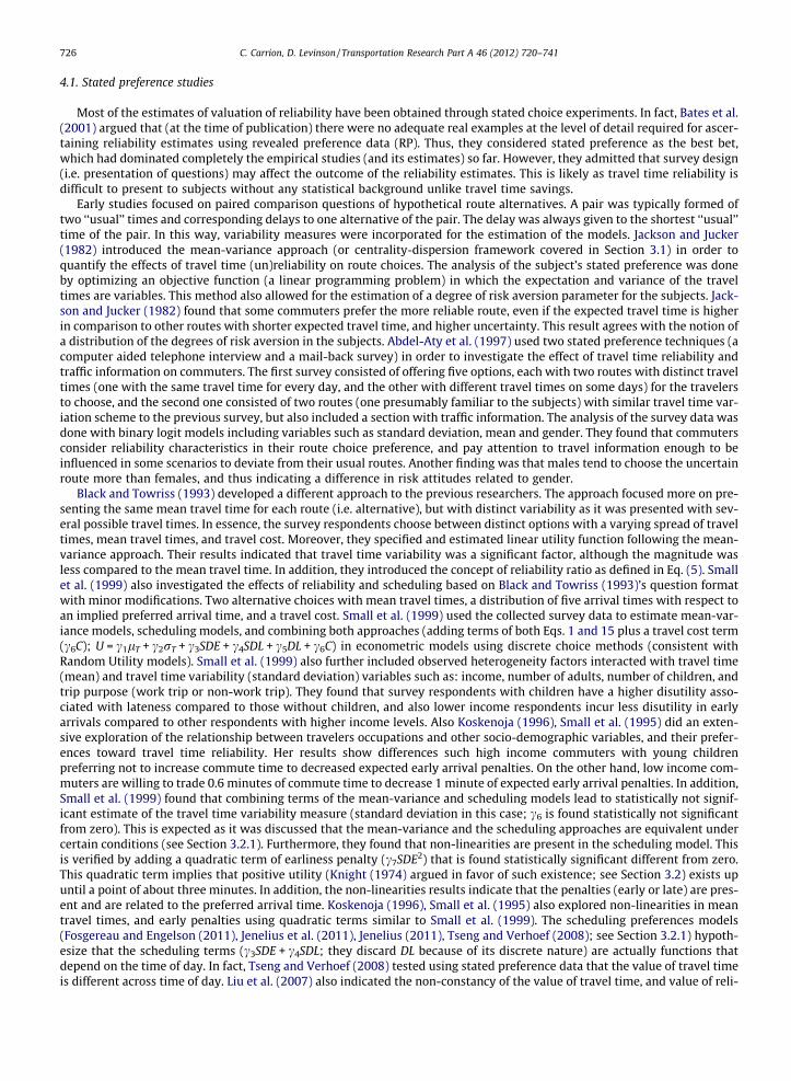
Early studies focused on paired comparison questions of hypothetical route alternatives. A pair was typically formed oftwo ‘‘usual’’ times and corresponding delays to one alternative of the pair. The delay was always given to the shortest ‘‘usual’’time of the pair. In this way, variability measures were incorporated for the estimation of the models. Jackson and Jucker(1982) introduced the mean-variance approach (or centrality-dispersion framework covered in Section 3.1) in order toquantify the effects of travel time (un)reliability on route choices. The analysis of the subject’s stated preference was doneby optimizing an objective function (a linear programming problem) in which the expectation and variance of the traveltimes are variables. This method also allowed for the estimation of a degree of risk aversion parameter for the subjects. Jack-son and Jucker (1982) found that some commuters prefer the more reliable route, even if the expected travel time is higherin comparison to other routes with shorter expected travel time, and higher uncertainty. This result agrees with the notion ofa distribution of the degrees of risk aversion in the subjects. Abdel-Aty et al. (1997) used two stated preference techniques (acomputer aided telephone interview and a mail-back survey) in order to investigate the effect of travel time reliability andtraffic information on commuters. The first survey consisted of offering five options, each with two routes with distinct traveltimes (one with the same travel time for every day, and the other with different travel times on some days) for the travelersto choose, and the second one consisted of two routes (one presumably familiar to the subjects) with similar travel time var-iation scheme to the previous survey, but also included a section with traffic information. The analysis of the survey data wasdone with binary logit models including variables such as standard deviation, mean and gender. They found that commutersconsider reliability characteristics in their route choice preference, and pay attention to travel information enough to beinfluenced in some scenarios to deviate from their usual routes. Another finding was that males tend to choose the uncertainroute more than females, and thus indicating a difference in risk attitudes related to gender.

Black and Towriss (1993) developed a different approach to the previous researchers. The approach focused more on pre-senting the same mean travel time for each route (i.e. alternative), but with distinct variability as it was presented with sev-eral possible travel times. In essence, the survey respondents choose between distinct options with a varying spread of traveltimes, mean travel times, and travel cost. Moreover, they specified and estimated linear utility function following the mean-variance approach. Their results indicated that travel time variability was a significant factor, although the magnitude wasless compared to the mean travel time. In addition, they introduced the concept of reliability ratio as defined in Eq. (5). Smallet al. (1999) also investigated the effects of reliability and scheduling based on Black and Towriss (1993)’s question formatwith minor modifications. Two alternative choices with mean travel times, a distribution of five arrival times with respect toan implied preferred arrival time, and a travel cost. Small et al. (1999) used the collected survey data to estimate mean-var-iance models, scheduling models, and combining both approaches (adding terms of both Eqs. 1 and 15 plus a travel cost term(c6C); U = c1lT + c2rT + c3SDE + c4SDL + c5DL + c6C) in econometric models using discrete choice methods (consistent withRandom Utility models). Small et al. (1999) also further included observed heterogeneity factors interacted with travel time(mean) and travel time variability (standard deviation) variables such as: income, number of adults, number of children, andtrip purpose (work trip or non-work trip). They found that survey respondents with children have a higher disutility asso-ciated with lateness compared to those without children, and also lower income respondents incur less disutility in earlyarrivals compared to other respondents with higher income levels. Also Koskenoja (1996), Small et al. (1995) did an exten-sive exploration of the relationship between travelers occupations and other socio-demographic variables, and their prefer-ences toward travel time reliability. Her results show differences such high income commuters with young childrenpreferring not to increase commute time to decreased expected early arrival penalties. On the other hand, low income com-muters are willing to trade 0.6 minutes of commute time to decrease 1 minute of expected early arrival penalties. In addition,Small et al. (1999) found that combining terms of the mean-variance and scheduling models lead to statistically not signif-icant estimate of the travel time variability measure (standard deviation in this case; c6 is found statistically not significantfrom zero). This is expected as it was discussed that the mean-variance and the scheduling approaches are equivalent undercertain conditions (see Section 3.2.1). Furthermore, they found that non-linearities are present in the scheduling model. Thisis verified by adding a quadratic term of earliness penalty (c7SDE2) that is found statistically significant different from zero.This quadratic term implies that positive utility (Knight (1974) argued in favor of such existence; see Section 3.2) exists upuntil a point of about three minutes. In addition, the non-linearities results indicate that the penalties (early or late) are pres-ent and are related to the preferred arrival time. Koskenoja (1996), Small et al. (1995) also explored non-linearities in meantravel times, and early penalties using quadratic terms similar to Small et al. (1999). The scheduling preferences models(Fosgereau and Engelson (2011), Jenelius et al. (2011), Jenelius (2011), Tseng and Verhoef (2008); see Section 3.2.1) hypoth-esize that the scheduling terms (c3SDE + c4SDL; they discard DL because of its discrete nature) are actually functions thatdepend on the time of day. In fact, Tseng and Verhoef (2008) tested using stated preference data that the value of travel timeis different across time of day. Liu et al. (2007) also indicated the non-constancy of the value of travel time, and value of reli-


ability using loop detector data. Therefore, it can be argued that non-linearities are starting to be considered in the recentmathematical models of scheduling preferences.

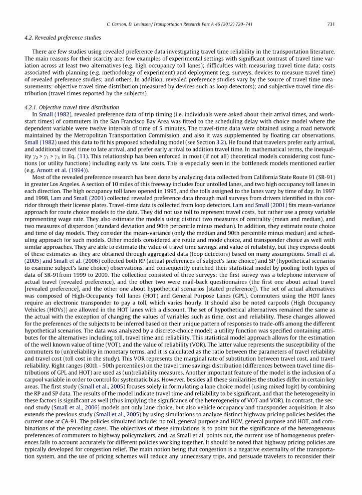
In the late 1990s and 2000s, the stated preference research focused on designing better presentations of questions aboutvariability. Cook et al. (1999) and Bates et al. (2001) asserted that the presentation of variability in the questions has a sig-nificant impact in the estimates, because of a mismatch between the respondents and analysts understanding of the abstractsituation. Thus, analysts must validate the understanding of their questionnaires with the survey respondents. Bates et al.(2001) and Cook et al. (1999) verified the understanding of respondents by presenting closely matching pairs of questions.They found that about 90% of respondents correctly identified the differences in the questions, except in cases where zerodelay was included, and respondents will choose the more variable (less reliable) alternative of the pair. Bates et al. (2001)and Cook et al. (1999) proposed an alternative design for the presentation of variability. This design consists of circulararrangement of arrival times with respect to a given preferred arrival time. Each arrival time is represented by a box indi-cating how many minutes early or late the respondent will arrive. Bates et al. (2001) and Cook et al. (1999) included edu-cation phases to increase the likelihood of survey respondents understanding of their circular presentation. Copley et al.(2002) studied different presentations (linear arrangements of possible travel times, circular arrangements of possible traveltimes, and histogram representation of possible travel times) of travel time variability. A qualitative approach by interview-ing respondents suggested a preference for linear arrangements and histograms presentations of variability. Copley et al.(2002) prefer the histogram representation, because it can present a large volume of information, and their qualitativeresearch showed that it was understood with little effort.

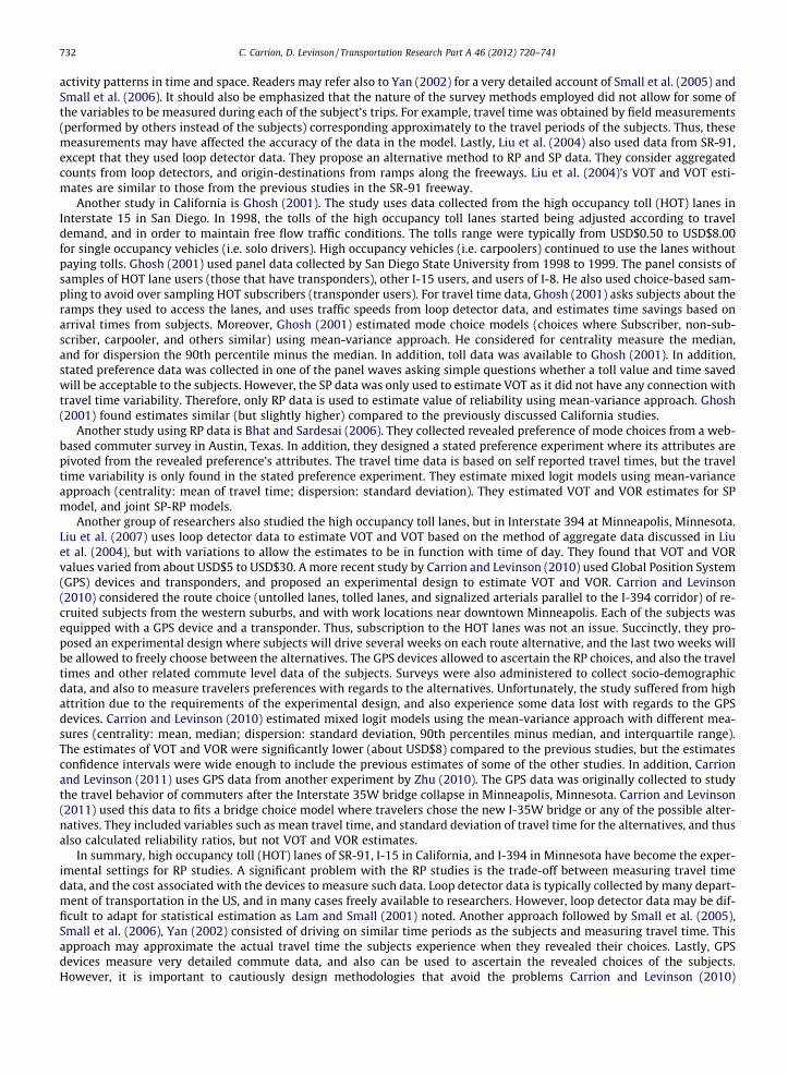
Other researchers also tried alternative presentations. Hensher (2001) used bar diagrams dividing the total travel timeinto: free flow, slowed down, stop/start, and uncertainty. The bars also provided numbers for the amount of minutes of eachcomponent of the total travel time for pairs of alternatives. The alternatives also included a travel cost component in order tocalculate trade offs between cost and the distinct components of time. It should be noted that Hensher (2001) was more con-cerned with investigating the values that travelers assign to the distinct components of the total travel time rather than tra-vel time reliability. Also, the uncertainty component is actually more closely related to the schedule delays (allocated extratime to avoid arriving late) rather than measures of the travel time variability (e.g. standard deviation). Hollander (2006)uses a very different presentation compared to the previous discussed researchers. Hollander (2006)’s survey design consistsof five bars per alternative indicating the time of departure (e.g. 8:15) on the top of the bar, and the time of arrival at thebottom of the bar (e.g. 8:30). In this way, travel times are not given in terms of minutes explicitly. In addition, travelersare told the time they should be at their destinations, explitcitly. Hollander (2006) estimated a scheduling model, and amean-variance model. The results indicate that the reliability ratio was vey low 0.1 (this is significantly small comparedto most studies) in the mean-variance model, and most users were willing to pay more to avoid arriving late in the sched-uling model. Asensio and Matas (2008) uses a similar presentation of variability as Small et al. (1999) (average travel time,and a distribution of possible travel times). Asensio and Matas (2008) also tests scheduling and mean-variance models. Theyfind that the inclusion of the variability measure plus scheduling delay measures resulted in lost of statistical significance inthe reliability variables of both models with the exception of schedule delay late. Thus, indicating a correlation between bothapproaches as theoretically expected, and already discussed. Tilahun and Levinson (2010) introduces a variability formatconsisting of a histogram for each alternative in a pair. They also introduce an education phase to explain to survey respon-dents what the histograms convey. They test a mode-variance model (mode is the most frequent travel time shown in thehistograms), mode-right range (100th percentile–50th percentile), and introduce a new measure consisting of two moments(one representing earliness, and another lateness). Tilahun and Levinson (2010) found a reliability ratio of 0.89 for the mode-variance model. They also found that survey respondents value lateness (in their proposed measure) similarly to travel timesavings. Li et al. (2010) introduce two distinct questionnaires representing variability based on Hensher (2001) and Smallet al. (1999). The first questionnaire contains three sections: average travel time experience, probability of time of arrival,and trip costs. The first section presents a division of average travel time very similar to Hensher (2001). The second sectionpresents the arrival time with respect to a implied preferred arrival time very similar to Small et al. (1999) distribution ofarrivals. The third section includes travel costs; a running cost is presented in addition to tolls costs. The second question-naire is similar to the first questionnaire, except that the sections are not divided, and the distribution of arrival times is re-placed with a row indicating the trip time variability (i.e. amount of minutes plus or less with respect to the travel time).Travel costs are presented as taxi fares, and toll costs. Li et al. (2010) tested the questionnaires with commuters andnon-commuters, and found that non-commuters values less travel time savings, lateness penalties, and travel time reliabilityrelative to commuters. The non-commuters’ reliability ratio is higher compared to commuters. In addition, Li et al. (2010)argued that the survey design similar to Small et al. (1999) (first questionnaire) is better understood by survey respondentsin comparison to the survey design similar to Jackson and Jucker (1982) (second questionnaire). It should be noted that thereare differences between Li et al. (2010)’s second questionnaire and Jackson and Jucker (1982)’s questionnaire even though Liet al. (2010) considers them as similar. An important difference is that Jackson and Jucker (1982) presents variability asnumber of additional minutes of delay per week, and Li et al. (2010) presents delays by plus or less minutes with respectto the travel time.

An important contribution to the design of stated preference surveys for analyzing travel time variability is Tseng et al.(2009). They use face-to-face interviews to investigate the understanding of subjects with most of the previously discussedquestionnaires (Bates et al. (2001), Copley et al. (2002), Hollander (2006), Small et al. (1999)). The analysis consisted of ques-tions about the respondents subjective preferences with regards to the formats, and questions that tested for consistency


and logic the perception of respondents with regards to reliability presented in the questionnaires. Tseng et al. (2009) foundthat Small et al. (1999)’s format is preferred, and understood by most of the respondents. Copley et al. (2002)’s formatshowed signs of difficulty in understanding the probabilities from the graph by some of the respondents. Hollander(2006)’s format received mixed results. Tseng et al. (2009) recommends not using this format. In addition, Bates et al.(2001)’s format was not preferred compared to other formats by respondents.

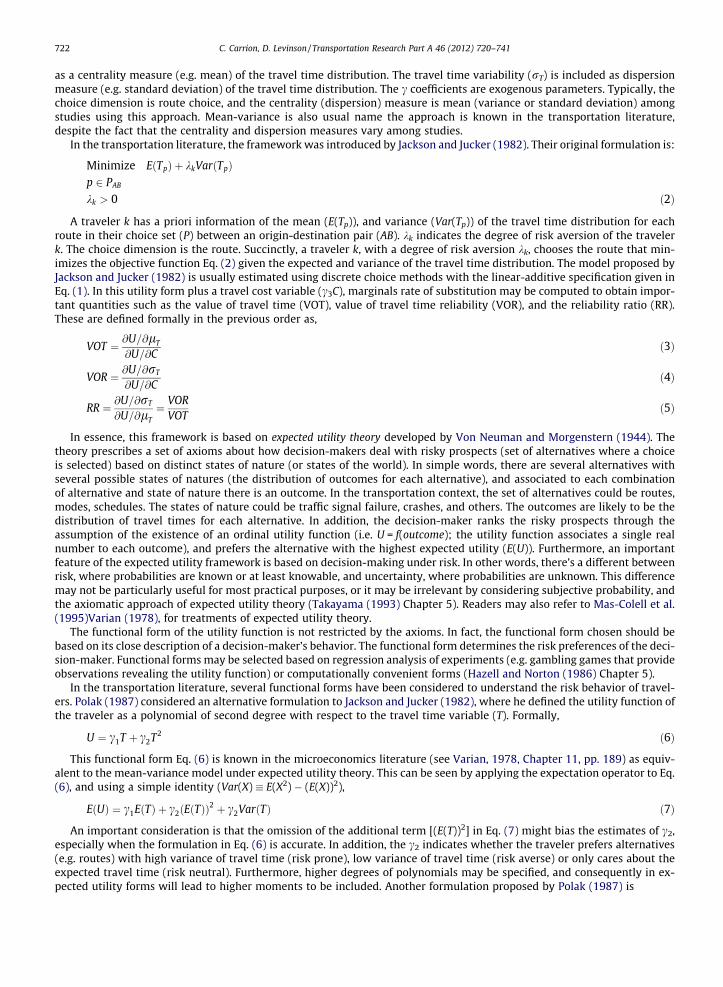
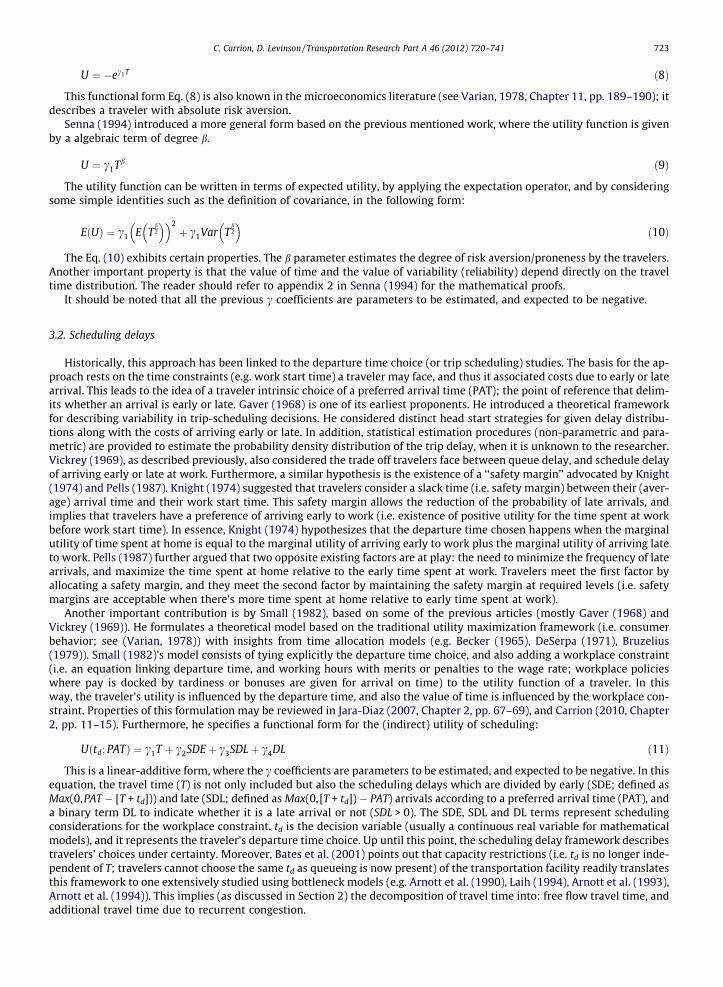
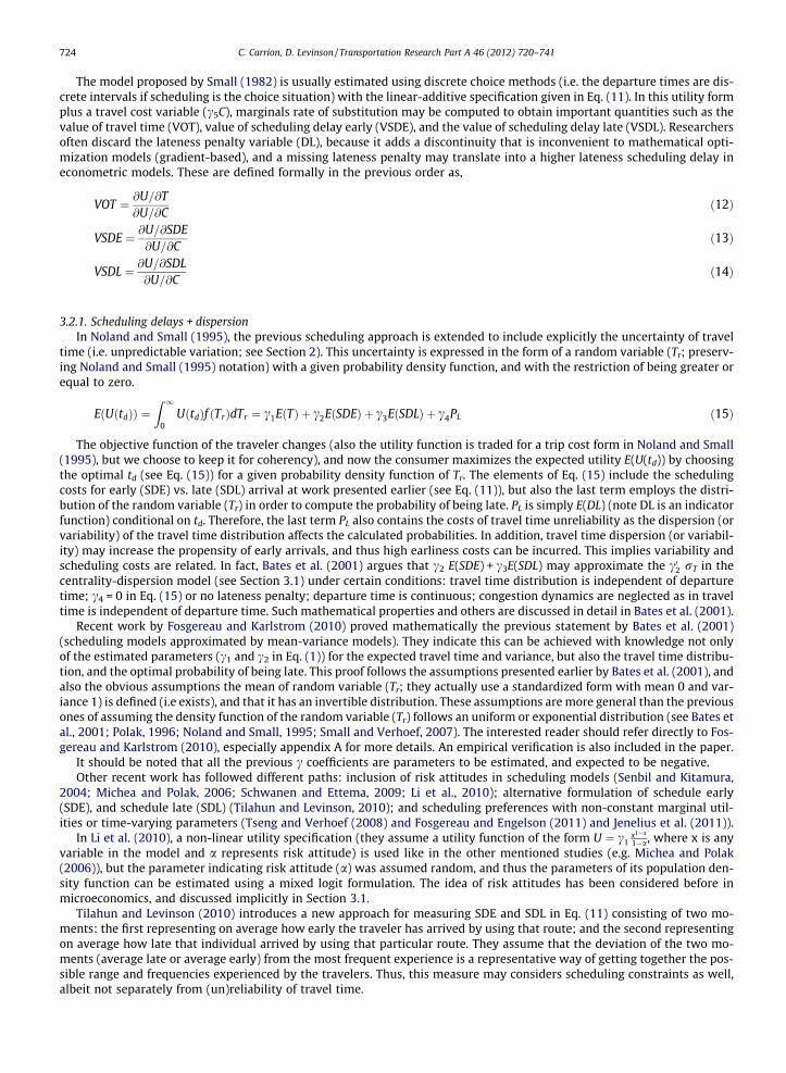
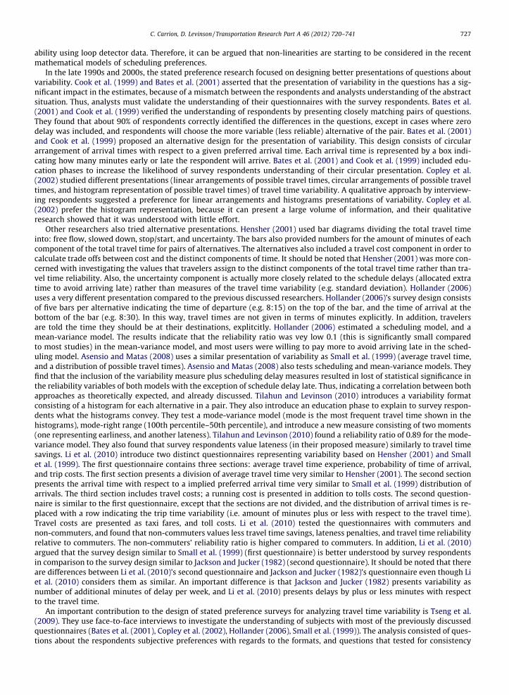
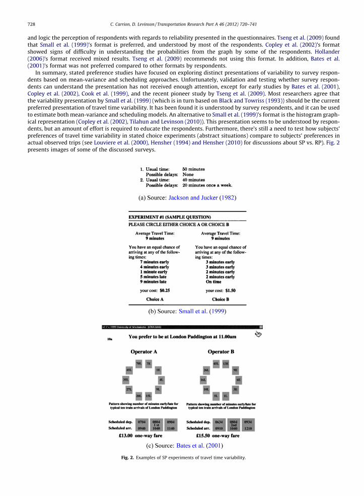
In summary, stated preference studies have focused on exploring distinct presentations of variability to survey respon-dents based on mean-variance and scheduling approaches. Unfortunately, validation and testing whether survey respon-dents can understand the presentation has not received enough attention, except for early studies by Bates et al. (2001),Copley et al. (2002), Cook et al. (1999), and the recent pioneer study by Tseng et al. (2009). Most researchers agree thatthe variability presentation by Small et al. (1999) (which is in turn based on Black and Towriss (1993)) should be the currentpreferred presentation of travel time variability. It has been found it is understood by survey respondents, and it can be usedto estimate both mean-variance and scheduling models. An alternative to Small et al. (1999)’s format is the histogram graph-ical representation (Copley et al. (2002), Tilahun and Levinson (2010)). This presentation seems to be understood by respon-dents, but an amount of effort is required to educate the respondents. Furthermore, there’s still a need to test how subjects’preferences of travel time variability in stated choice experiments (abstract situations) compare to subjects’ preferences inactual observed trips (see Louviere et al. (2000), Hensher (1994) and Hensher (2010) for discussions about SP vs. RP). Fig. 2presents images of some of the discussed surveys.

Fig. 2. Examples of SP experiments of travel time variability.

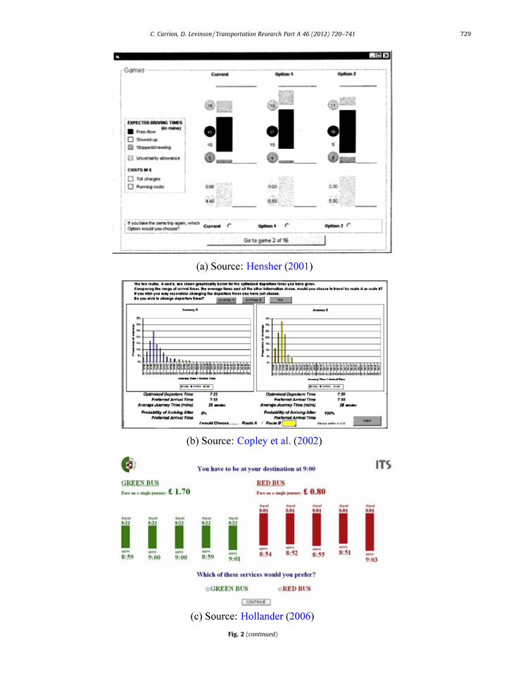
Fig. 2 (continued)


Fig. 2 (continued)



4.2. Revealed preference studies

There are few studies using revealed preference data investigating travel time reliability in the transportation literature.The main reasons for their scarcity are: few examples of experimental settings with significant contrast of travel time var-iation across at least two alternatives (e.g. high occupancy toll lanes); difficulties with measuring travel time data; costsassociated with planning (e.g. methodology of experiment) and deployment (e.g. surveys, devices to measure travel time)of revealed preference studies; and others. In addition, revealed preference studies vary by the source of travel time mea-surements: objective travel time distribution (measured by devices such as loop detectors); and subjective travel time dis-tribution (travel times reported by the subjects).

4.2.1. Objective travel time distributionIn Small (1982), revealed preference data of trip timing (i.e. individuals were asked about their arrival times, and work-

start times) of commuters in the San Francisco Bay Area was fitted to the scheduling delay with choice model where thedependent variable were twelve intervals of time of 5 minutes. The travel-time data were obtained using a road networkmaintained by the Metropolitan Transportation Commission, and also it was supplemented by floating car observations.Small (1982) used this data to fit his proposed scheduling model (see Section 3.2). He found that travelers prefer early arrival,and additional travel time to late arrival, and prefer early arrival to addition travel time. In mathematical terms, the inequal-ity c2 > c1 > c3 in Eq. (11). This relationship has been enforced in most (if not all) theoretical models considering cost func-tions (or utility functions) including early vs. late costs. This is especially seen in the bottleneck models mentioned earlier(e.g. Arnott et al. (1994)).

Most of the revealed preference research has been done by analyzing data collected from California State Route 91 (SR-91)in greater Los Angeles. A section of 10 miles of this freeway includes four untolled lanes, and two high occupancy toll lanes ineach direction. The high occupancy toll lanes opened in 1995, and the tolls assigned to the lanes vary by time of day. In 1997and 1998, Lam and Small (2001) collected revealed preference data through mail surveys from drivers identified in this cor-ridor through their license plates. Travel-time data is collected from loop detectors. Lam and Small (2001) fits mean-varianceapproach for route choice models to the data. They did not use toll to represent travel costs, but rather use a proxy variablerepresenting wage rate. They also estimate the models using distinct two measures of centrality (mean and median), andtwo measures of dispersion (standard deviation and 90th percentile minus median). In addition, they estimate route choiceand time of day models. They consider the mean-variance (only the median and 90th percentile minus median) and sched-uling approach for such models. Other models considered are route and mode choice, and transponder choice as well withsimilar approaches. They are able to estimate the value of travel time savings, and value of reliability, but they express doubtof these estimates as they are obtained through aggregated data (loop detectors) based on many assumptions. Small et al.(2005) and Small et al. (2006) collected both RP (actual preferences of subject’s lane choice) and SP (hypothetical scenariosto examine subject’s lane choice) observations, and consequently enriched their statistical model by pooling both types ofdata of SR-91from 1999 to 2000. The collection consisted of three surveys: the first survey was a telephone interview ofactual travel (revealed preference), and the other two were mail-back questionnaires (the first one about actual travel[revealed preference], and the other one about hypothetical scenarios [stated preference]). The set of actual alternativeswas composed of High-Occupancy Toll lanes (HOT) and General Purpose Lanes (GPL). Commuters using the HOT lanesrequire an electronic transponder to pay a toll, which varies hourly. It should also be noted carpools (High OccupancyVehicles (HOVs)) are allowed in the HOT lanes with a discount. The set of hypothetical alternatives remained the same asthe actual with the exception of changing the values of variables such as time, cost and reliability. These changes allowedfor the preferences of the subjects to be inferred based on their unique pattern of responses to trade-offs among the differenthypothetical scenarios. The data was analyzed by a discrete-choice model; a utility function was specified containing attri-butes for the alternatives including toll, travel time and reliability. This statistical model approach allows for the estimationof the well known value of time (VOT), and the value of reliability (VOR). The latter value represents the susceptibility of thecommuters to (un)reliability in monetary terms, and it is calculated as the ratio between the parameters of travel reliabilityand travel cost (toll cost in the study). This VOR represents the marginal rate of substitution between travel cost, and travelreliability. Right ranges (80th - 50th percentiles) on the travel time savings distribution (differences between travel time dis-tributions of GPL and HOT) are used as (un)reliability measures. Another important feature of the model is the inclusion of acarpool variable in order to control for systematic bias. However, besides all these similarities the studies differ in certain keyareas. The first study (Small et al., 2005) focuses solely in formulating a lane choice model (using mixed logit) by combiningthe RP and SP data. The results of the model indicate travel time and reliability to be significant, and that the heterogeneity inthese factors is significant as well (thus implying the significance of the heterogeneity of VOT and VOR). In contrast, the sec-ond study (Small et al., 2006) models not only lane choice, but also vehicle occupancy and transponder acquisition. It alsoextends the previous study (Small et al., 2005) by using simulations to analyze distinct highway pricing policies besides thecurrent one at CA-91. The policies simulated include: no toll, general purpose and HOV, general purpose and HOT, and com-binations of the preceding cases. The objectives of these simulations is to point out the significance of the heterogeneouspreferences of commuters to highway policymakers, and, as Small et al. points out, the current use of homogeneous prefer-ences fails to account accurately for different policies working together. It should be noted that highway pricing policies aretypically developed for congestion relief. The main notion being that congestion is a negative externality of the transporta-tion system, and the use of pricing schemes will reduce any unnecessary trips, and persuade travelers to reconsider their


activity patterns in time and space. Readers may refer also to Yan (2002) for a very detailed account of Small et al. (2005) andSmall et al. (2006). It should also be emphasized that the nature of the survey methods employed did not allow for some ofthe variables to be measured during each of the subject’s trips. For example, travel time was obtained by field measurements(performed by others instead of the subjects) corresponding approximately to the travel periods of the subjects. Thus, thesemeasurements may have affected the accuracy of the data in the model. Lastly, Liu et al. (2004) also used data from SR-91,except that they used loop detector data. They propose an alternative method to RP and SP data. They consider aggregatedcounts from loop detectors, and origin-destinations from ramps along the freeways. Liu et al. (2004)’s VOT and VOT esti-mates are similar to those from the previous studies in the SR-91 freeway.

Another study in California is Ghosh (2001). The study uses data collected from the high occupancy toll (HOT) lanes inInterstate 15 in San Diego. In 1998, the tolls of the high occupancy toll lanes started being adjusted according to traveldemand, and in order to maintain free flow traffic conditions. The tolls range were typically from USD$0.50 to USD$8.00for single occupancy vehicles (i.e. solo drivers). High occupancy vehicles (i.e. carpoolers) continued to use the lanes withoutpaying tolls. Ghosh (2001) used panel data collected by San Diego State University from 1998 to 1999. The panel consists ofsamples of HOT lane users (those that have transponders), other I-15 users, and users of I-8. He also used choice-based sam-pling to avoid over sampling HOT subscribers (transponder users). For travel time data, Ghosh (2001) asks subjects about theramps they used to access the lanes, and uses traffic speeds from loop detector data, and estimates time savings based onarrival times from subjects. Moreover, Ghosh (2001) estimated mode choice models (choices where Subscriber, non-sub-scriber, carpooler, and others similar) using mean-variance approach. He considered for centrality measure the median,and for dispersion the 90th percentile minus the median. In addition, toll data was available to Ghosh (2001). In addition,stated preference data was collected in one of the panel waves asking simple questions whether a toll value and time savedwill be acceptable to the subjects. However, the SP data was only used to estimate VOT as it did not have any connection withtravel time variability. Therefore, only RP data is used to estimate value of reliability using mean-variance approach. Ghosh(2001) found estimates similar (but slightly higher) compared to the previously discussed California studies.

Another study using RP data is Bhat and Sardesai (2006). They collected revealed preference of mode choices from a web-based commuter survey in Austin, Texas. In addition, they designed a stated preference experiment where its attributes arepivoted from the revealed preference’s attributes. The travel time data is based on self reported travel times, but the traveltime variability is only found in the stated preference experiment. They estimate mixed logit models using mean-varianceapproach (centrality: mean of travel time; dispersion: standard deviation). They estimated VOT and VOR estimates for SPmodel, and joint SP-RP models.

Another group of researchers also studied the high occupancy toll lanes, but in Interstate 394 at Minneapolis, Minnesota.Liu et al. (2007) uses loop detector data to estimate VOT and VOT based on the method of aggregate data discussed in Liuet al. (2004), but with variations to allow the estimates to be in function with time of day. They found that VOT and VORvalues varied from about USD$5 to USD$30. A more recent study by Carrion and Levinson (2010) used Global Position System(GPS) devices and transponders, and proposed an experimental design to estimate VOT and VOR. Carrion and Levinson(2010) considered the route choice (untolled lanes, tolled lanes, and signalized arterials parallel to the I-394 corridor) of re-cruited subjects from the western suburbs, and with work locations near downtown Minneapolis. Each of the subjects wasequipped with a GPS device and a transponder. Thus, subscription to the HOT lanes was not an issue. Succinctly, they pro-posed an experimental design where subjects will drive several weeks on each route alternative, and the last two weeks willbe allowed to freely choose between the alternatives. The GPS devices allowed to ascertain the RP choices, and also the traveltimes and other related commute level data of the subjects. Surveys were also administered to collect socio-demographicdata, and also to measure travelers preferences with regards to the alternatives. Unfortunately, the study suffered from highattrition due to the requirements of the experimental design, and also experience some data lost with regards to the GPSdevices. Carrion and Levinson (2010) estimated mixed logit models using the mean-variance approach with different mea-sures (centrality: mean, median; dispersion: standard deviation, 90th percentiles minus median, and interquartile range).The estimates of VOT and VOR were significantly lower (about USD$8) compared to the previous studies, but the estimatesconfidence intervals were wide enough to include the previous estimates of some of the other studies. In addition, Carrionand Levinson (2011) uses GPS data from another experiment by Zhu (2010). The GPS data was originally collected to studythe travel behavior of commuters after the Interstate 35W bridge collapse in Minneapolis, Minnesota. Carrion and Levinson(2011) used this data to fits a bridge choice model where travelers chose the new I-35W bridge or any of the possible alter-natives. They included variables such as mean travel time, and standard deviation of travel time for the alternatives, and thusalso calculated reliability ratios, but not VOT and VOR estimates.

In summary, high occupancy toll (HOT) lanes of SR-91, I-15 in California, and I-394 in Minnesota have become the exper-imental settings for RP studies. A significant problem with the RP studies is the trade-off between measuring travel timedata, and the cost associated with the devices to measure such data. Loop detector data is typically collected by many depart-ment of transportation in the US, and in many cases freely available to researchers. However, loop detector data may be dif-ficult to adapt for statistical estimation as Lam and Small (2001) noted. Another approach followed by Small et al. (2005),Small et al. (2006), Yan (2002) consisted of driving on similar time periods as the subjects and measuring travel time. Thisapproach may approximate the actual travel time the subjects experience when they revealed their choices. Lastly, GPSdevices measure very detailed commute data, and also can be used to ascertain the revealed choices of the subjects.However, it is important to cautiously design methodologies that avoid the problems Carrion and Levinson (2010)


experienced. Furthermore, the mean-variance approach dominates the RP models (except for Lam and Small (2001)),because most likely preferred arrival times of the subjects were not collected.

4.2.2. Subjective travel time distributionUp until this point, it has been assumed that travelers choose optimally under the objective travel time distribution (i.e.

the perception error of travelers is close to zero). Bates et al. (2001) argues that it is likely travelers are optimizing accordingto their own divergent view of the objective distribution (i.e. based on actual measurements). Consequently, travelers willdiffer in their optimal solutions depending on the degree of distortion of their subjective distribution with regards to theobjective distribution. This very likely as it has been shown in the transportation literature for different types of travel timesuch as waiting time (examples include Levinson et al. (2006), Levinson et al. (2004)). In this way, it is reasonable that therandom variable representing subjective travel time (Ts) can be decomposed as: a random variable representing objectivetravel time (To), and a random perception error or distortion variable (D). In other words, Ts = To + D. The probability densityfunction of Ts can be obtained by solving a convolution integral (assuming independence) or, more general (assuming noindependence), by solving the joint distribution integral (with its respective Jacobian of the transformation) as long as weknow the probability density functions of To and D. Furthermore, the parameters of the probability density functions ofTo, and D could be estimated given the ‘‘proper’’ data. By ‘‘proper’’, it refers to for example individual experienced travel timemeasurements in order to estimate the traveler’s objective travel time distribution. In the case of the distortion distribution,the method is not so obvious.

Recently, Peer et al. (2010) studied the travelers’ perception of their morning commute. Basically, they compared reportedtravel times by subjects from questionnaires, and compared them to their travel times from camera data. In essence, theycompared reported travel time distributions (subjective) to camera travel time distributions (objective). They found that cer-tainly perception error is an issue that need to be taken in consideration. This result should be emphasized as more RP stud-ies may be underestimating or overestimating the value of time, and value of reliability as the objective travel timedistributions differ to subjective travel time distributions. In other words, travelers may see worthwhile savings and predict-ability (low variability) that do not match the actual savings and predictability (low variability).

5. Meta-analysis

In other fields (mainly in social sciences), meta-analysis has been used to analyze and summarize the results of variousstudies. This method analyses data at a higher level; it searches for patterns in the results of other studies through statisticaltools (e.g. meta-regression). Furthermore, these patterns (or differences) can be understood with the use of several regres-sors incorporating several key characteristics (e.g. regional variables) of each study. There are several advantages and disad-vantages with meta-analysis that need to be taken in consideration. These are briefly discussed subsequently. Also, seeGuzzo et al. (1987) and Arnqvist and Wooster (1995) for more details.

Several of the advantages of meta-analysis include:

� It identifies general patterns that may have been overlooked by conventional reviews.� It provides objective evidence of the state of the research.� It allows to control for between-study variations.� Statistical power to detect an effect from the population of studies.

Several of the disadvantages of meta-analysis include:

� Many studies must be selected in order to reduce the bias of the authors for certain studies� Ignoring the possible effects of study characteristics.

6. Data

A data set was assembled after an extensive search of studies with comparable estimates and methodology in transpor-tation research journals, Google (scholar) search engine, and other articles’ databases. Empirical studies were includedaccording to the following criteria:

� Contained estimates of VOT, VOR, or RR that could be made comparable across studies;� Stated explicitly and clearly how the expected travel time and travel time (un)reliability were measured;� Sample size of the data was provided;

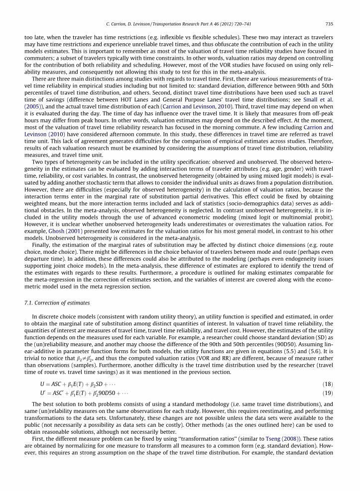
Table 1 presents the studies selected for the meta-analysis. Data Type refers to Stated Preference (SP), or Revealed Pref-erence (RP) or both. Observations refers to the number of Reliability Ratio (RR) estimates available in each study, and theaverage of RR provides the mean among those observations. Maximum and Minimum values are included as well. Fig. 3 pre-sents the reliability ratios found in the studies selected for the meta-analysis.

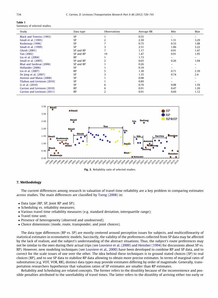
Table 1Summary of selected studies.

Study Data type Observations Average RR Min Max

Black and Towriss (1993) SP 1 0.55 – –Small et al. (1995) SP 2 2.30 1.31 3.29Koskenoja (1996) SP 7 0.75 0.33 1.08Small et al. (1999) SP 3 2.51 1.86 3.22Ghosh (2001) SP and RP 7 1.17 0.91 1.47Yan (2002) SP and RP 19 1.47 0.91 1.95Liu et al. (2004) RP 1 1.73 – –Small et al. (2005) SP and RP 2 0.65 0.26 1.04Bhat and Sardesai (2006) SP and RP 1 0.26 – –Hollander (2006) SP 1 0.10 – –Liu et al. (2007) RP 5 1.30 0.71 2.39De Jong et al. (2007) SP 3 1.35 0.74 2.4Asensio and Matas (2008) SP 1 0.98 – –Tilahun and Levinson (2010) SP 1 0.89 – –Li et al. (2010) SP 6 0.70 0.08 1.59Carrion and Levinson (2010) RP 6 0.91 0.47 1.20Carrion and Levinson (2011) RP 2 0.91 0.69 1.12

Fig. 3. Reliability ratio of selected studies.


7. Methodology

The current differences among research in valuation of travel time reliability are a key problem in comparing estimatesacross studies. The main differences are classified by Tseng (2008) in:

� Data type (RP, SP, Joint RP and SP);� Scheduling vs. reliability measures;� Various travel time reliability measures (e.g. standard deviation, interquartile range);� Travel time unit;� Presence of heterogeneity (observed and unobserved);� Choice dimensions (mode, route, transponder, and joint choices).

The data type differences (RP vs. SP) are mostly centered around perception issues for subjects, and multicollinearity ofstatistical estimates in econometric models. Succinctly, the validity of the preferences collected from SP data may be affectedby the lack of realism, and the subject’s understanding of the abstract situations. Thus, the subject’s route preferences maynot be similar to the ones during their actual trips (see Louviere et al. (2000) and Hensher (1994) for discussions about SP vs.RP). However, new modeling techniques (see Louviere et al., 2000) have been developed to combine RP and SP data, and tocorrect for the scale issues of one over the other. The idea behind these techniques is to ground stated choices (SP) to realchoices (RP), and to use SP data to stabilize RP data allowing to obtain more precise estimates. In terms of marginal rates ofsubstitution (e.g. VOT, VOR, RR), distinct data types may provide estimates differing by order of magnitude. Generally, trans-portation researchers hypothesize that valuation ratios of SP estimates are smaller than RP estimates.

Reliability and Scheduling are related concepts. The former refers to the disutility because of the inconvenience and pos-sible penalties attributed to the unreliability of travel times. The latter refers to the disutility of arriving either too early or


too late, when the traveler has time restrictions (e.g. inflexible vs flexible schedules). These two may interact as travelersmay have time restrictions and experience unreliable travel times, and thus obfuscate the contribution of each in the utilitymodels estimates. This is important to remember as most of the valuation of travel time reliability studies have focused incommuters; a subset of travelers typically with time constraints. In other words, valuation ratios may depend on controllingfor the contribution of both reliability and scheduling. However, most of the VOR studies have focused on using only reli-ability measures, and consequently not allowing this study to test for this in the meta-analysis.

There are three main distinctions among studies with regards to travel time. First, there are various measurements of tra-vel time reliability in empirical studies including but not limited to: standard deviation, difference between 90th and 50thpercentiles of travel time distribution, and others. Second, distinct travel time distributions have been used such as traveltime of savings (difference between HOT Lanes and General Purpose Lanes’ travel time distributions; see Small et al.(2005)), and the actual travel time distribution of each (Carrion and Levinson, 2010). Third, travel time may depend on whenit is evaluated during the day. The time of day has influence over the travel time. It is likely that measures from off-peakhours may differ from peak hours. In other words, valuation estimates may depend on the described effect. At the moment,most of the valuation of travel time reliability research has focused in the morning commute. A few including Carrion andLevinson (2010) have considered afternoon commute. In this study, these differences in travel time are referred as traveltime unit. This lack of agreement generates difficulties for the comparison of empirical estimates across studies. Therefore,results of each valuation research must be examined by considering the assumptions of travel time distribution, reliabilitymeasures, and travel time unit.

Two types of heterogeneity can be included in the utility specification: observed and unobserved. The observed hetero-geneity in the estimates can be evaluated by adding interaction terms of traveler attributes (e.g. age, gender) with traveltime, reliability, or cost variables. In contrast, the unobserved heterogeneity (obtained by using mixed logit models) is eval-uated by adding another stochastic term that allows to consider the individual units as draws from a population distribution.However, there are difficulties (especially for observed heterogeneity) in the calculation of valuation ratios, because theinteraction terms enter in the marginal rate of substitution partial derivatives. This effect could be fixed by obtainingweighted means, but the more interaction terms included and lack of statistics (socio-demographics data) serves as addi-tional obstacles. In the meta-analysis, observed heterogeneity is neglected. In contrast unobserved heterogeneity, it is in-cluded in the utility models through the use of advanced econometric modeling (mixed logit or multinomial probit).However, it is unclear whether unobserved heterogeneity leads underestimates or overestimates the valuation ratios. Forexample, Ghosh (2001) presented low estimates for the valuation ratios for his most general model, in contrast to his othermodels. Unobserved heterogeneity is considered in the meta-analysis.

Finally, the estimation of the marginal rates of substitution may be affected by distinct choice dimensions (e.g. routechoice, mode choice). There might be differences in the choice behavior of travelers between mode and route (perhaps evendeparture time). In addition, these differences could also be attributed to the modeling (perhaps even endogeneity issuessupporting joint choice models). In the meta-analysis, these difference of estimates are explored to identify the trend ofthe estimates with regards to these results. Furthermore, a procedure is outlined for making estimates comparable forthe meta-regression in the correction of estimates section, and the variables of interest are covered along with the econo-metric model used in the meta regression section.

7.1. Correction of estimates

In discrete choice models (consistent with random utility theory), an utility function is specified and estimated, in orderto obtain the marginal rate of substitution among distinct quantities of interest. In valuation of travel time reliability, thequantities of interest are measures of travel time, travel time reliability, and travel cost. However, the estimates of the utilityfunction depends on the measures used for each variable. For example, a researcher could choose standard deviation (SD) asthe (un)reliability measure, and another may choose the difference of the 90th and 50th percentiles (90D50). Assuming lin-ear-additive in parameter function forms for both models, the utility functions are given in equations (5.5) and (5.6). It istrivial to notice that b2–b02, and thus the computed valuation ratios (VOR and RR) are different, because of measure ratherthan observations (samples). Furthermore, another difficulty is the travel time distribution used by the researcher (traveltime of route vs. travel time savings) as it was mentioned in the previous section.

U ¼ ASC þ b1EðTÞ þ b2SDþ � � � ð18ÞU0 ¼ ASC0 þ b01EðTÞ þ b0290D50þ � � � ð19Þ

The best solution to both problems consists of using a standard methodology (i.e. same travel time distributions), andsame (un)relability measures on the same observations for each study. However, this requires reestimating, and performingtransformations to the data sets. Unfortunately, these changes are not possible unless the data sets were available to thepublic (not necessarily a possibility as data sets can be costly). Other methods (as the ones outlined here) can be used toobtain reasonable solutions, although not necessarily better.

First, the different measure problem can be fixed by using ‘‘transformation ratios’’ (similar to Tseng (2008)). These ratiosare obtained by normalizing for one measure to transform all measures to a common form (e.g. standard deviation). How-ever, this requires an strong assumption on the shape of the travel time distribution. For example, the standard deviation

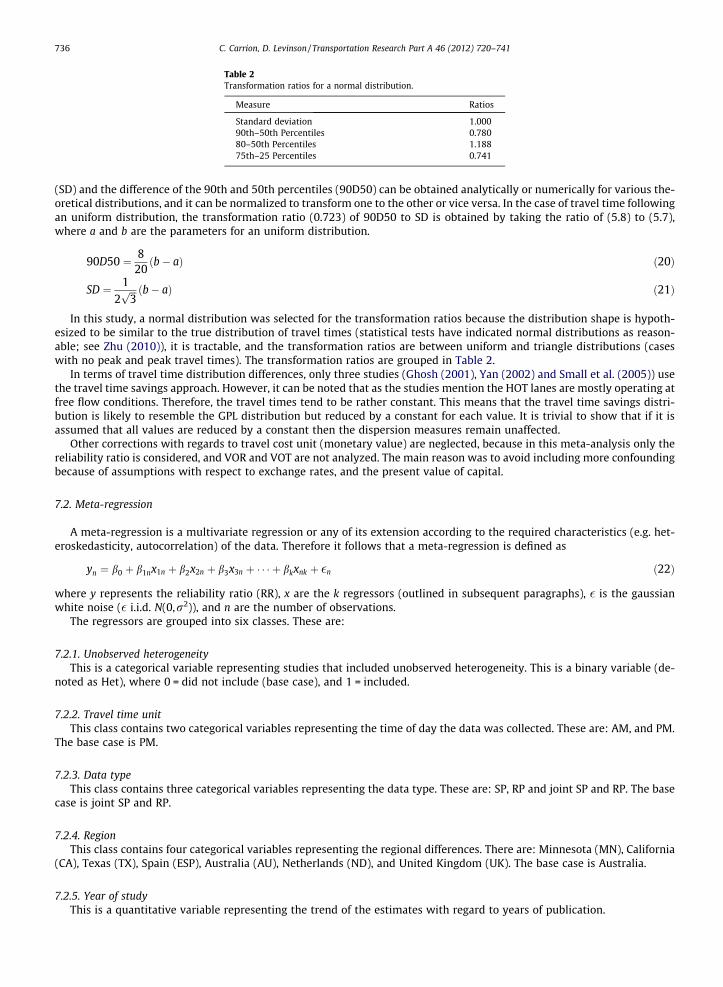
Table 2Transformation ratios for a normal distribution.

Measure Ratios

Standard deviation 1.00090th–50th Percentiles 0.78080–50th Percentiles 1.18875th–25 Percentiles 0.741


(SD) and the difference of the 90th and 50th percentiles (90D50) can be obtained analytically or numerically for various the-oretical distributions, and it can be normalized to transform one to the other or vice versa. In the case of travel time followingan uniform distribution, the transformation ratio (0.723) of 90D50 to SD is obtained by taking the ratio of (5.8) to (5.7),where a and b are the parameters for an uniform distribution.

90D50 ¼ 820ðb� aÞ ð20Þ

SD ¼ 12ffiffiffi3p ðb� aÞ ð21Þ

In this study, a normal distribution was selected for the transformation ratios because the distribution shape is hypoth-esized to be similar to the true distribution of travel times (statistical tests have indicated normal distributions as reason-able; see Zhu (2010)), it is tractable, and the transformation ratios are between uniform and triangle distributions (caseswith no peak and peak travel times). The transformation ratios are grouped in Table 2.

In terms of travel time distribution differences, only three studies (Ghosh (2001), Yan (2002) and Small et al. (2005)) usethe travel time savings approach. However, it can be noted that as the studies mention the HOT lanes are mostly operating atfree flow conditions. Therefore, the travel times tend to be rather constant. This means that the travel time savings distri-bution is likely to resemble the GPL distribution but reduced by a constant for each value. It is trivial to show that if it isassumed that all values are reduced by a constant then the dispersion measures remain unaffected.

Other corrections with regards to travel cost unit (monetary value) are neglected, because in this meta-analysis only thereliability ratio is considered, and VOR and VOT are not analyzed. The main reason was to avoid including more confoundingbecause of assumptions with respect to exchange rates, and the present value of capital.

7.2. Meta-regression

A meta-regression is a multivariate regression or any of its extension according to the required characteristics (e.g. het-eroskedasticity, autocorrelation) of the data. Therefore it follows that a meta-regression is defined as

yn ¼ b0 þ b1nx1n þ b2x2n þ b3x3n þ � � � þ bkxnk þ �n ð22Þ

where y represents the reliability ratio (RR), x are the k regressors (outlined in subsequent paragraphs), � is the gaussianwhite noise (� i.i.d. N(0,r2)), and n are the number of observations.

The regressors are grouped into six classes. These are:

7.2.1. Unobserved heterogeneityThis is a categorical variable representing studies that included unobserved heterogeneity. This is a binary variable (de-

noted as Het), where 0 = did not include (base case), and 1 = included.

7.2.2. Travel time unitThis class contains two categorical variables representing the time of day the data was collected. These are: AM, and PM.

The base case is PM.

7.2.3. Data typeThis class contains three categorical variables representing the data type. These are: SP, RP and joint SP and RP. The base

case is joint SP and RP.

7.2.4. RegionThis class contains four categorical variables representing the regional differences. There are: Minnesota (MN), California

(CA), Texas (TX), Spain (ESP), Australia (AU), Netherlands (ND), and United Kingdom (UK). The base case is Australia.

7.2.5. Year of studyThis is a quantitative variable representing the trend of the estimates with regard to years of publication.

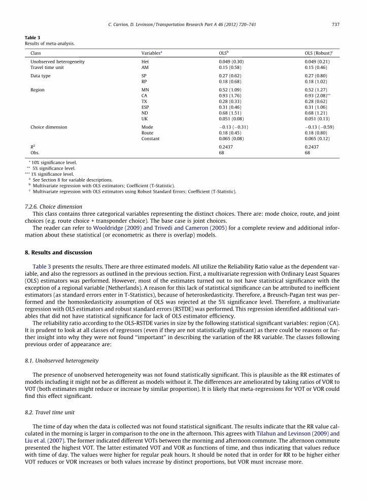
Table 3Results of meta-analysis.

Class Variablesa OLSb OLS (Robust)c

Unobserved heterogeneity Het 0.049 (0.30) 0.049 (0.21)Travel time unit AM 0.15 (0.58) 0.15 (0.46)

Data type SP 0.27 (0.62) 0.27 (0.80)RP 0.18 (0.68) 0.18 (1.02)

Region MN 0.52 (1.09) 0.52 (1.27)CA 0.93 (1.76) 0.93 (2.08)⁄⁄

TX 0.28 (0.33) 0.28 (0.62)ESP 0.31 (0.46) 0.31 (1.06)ND 0.68 (1.51) 0.68 (1.21)UK 0.051 (0.08) 0.051 (0.13)

Choice dimension Mode �0.13 (�0.31) �0.13 (�0.59)Route 0.18 (0.45) 0.18 (0.80)Constant 0.065 (0.08) 0.065 (0.12)

R2 0.2437 0.2437Obs. 68 68

⁄ 10% significance level.⁄⁄ 5% significance level.⁄⁄⁄ 1% significance level.

a See Section 8 for variable descriptions.b Multivariate regression with OLS estimators; Coefficient (T-Statistic).c Multivariate regression with OLS estimators using Robust Standard Errors; Coefficient (T-Statistic).


7.2.6. Choice dimensionThis class contains three categorical variables representing the distinct choices. There are: mode choice, route, and joint

choices (e.g. route choice + transponder choice). The base case is joint choices.The reader can refer to Wooldridge (2009) and Trivedi and Cameron (2005) for a complete review and additional infor-

mation about these statistical (or econometric as there is overlap) models.

8. Results and discussion

Table 3 presents the results. There are three estimated models. All utilize the Reliability Ratio value as the dependent var-iable, and also the regressors as outlined in the previous section. First, a multivariate regression with Ordinary Least Squares(OLS) estimators was performed. However, most of the estimates turned out to not have statistical significance with theexception of a regional variable (Netherlands). A reason for this lack of statistical significance can be attributed to inefficientestimators (as standard errors enter in T-Statistics), because of heteroskedasticity. Therefore, a Breusch-Pagan test was per-formed and the homoskedasticity assumption of OLS was rejected at the 5% significance level. Therefore, a multivariateregression with OLS estimators and robust standard errors (RSTDE) was performed. This regression identified additional vari-ables that did not have statistical significance for lack of OLS estimator efficiency.

The reliability ratio according to the OLS-RSTDE varies in size by the following statistical significant variables: region (CA).It is prudent to look at all classes of regressors (even if they are not statistically significant) as there could be reasons or fur-ther insight into why they were not found ‘‘important’’ in describing the variation of the RR variable. The classes followingprevious order of appearance are:

8.1. Unobserved heterogeneity

The presence of unobserved heterogeneity was not found statistically significant. This is plausible as the RR estimates ofmodels including it might not be as different as models without it. The differences are ameliorated by taking ratios of VOR toVOT (both estimates might reduce or increase by similar proportion). It is likely that meta-regressions for VOT or VOR couldfind this effect significant.

8.2. Travel time unit

The time of day when the data is collected was not found statistical significant. The results indicate that the RR value cal-culated in the morning is larger in comparison to the one in the afternoon. This agrees with Tilahun and Levinson (2009) andLiu et al. (2007). The former indicated different VOTs between the morning and afternoon commute. The afternoon commutepresented the highest VOT. The latter estimated VOT and VOR as functions of time, and thus indicating that values reducewith time of day. The values were higher for regular peak hours. It should be noted that in order for RR to be higher eitherVOT reduces or VOR increases or both values increase by distinct proportions, but VOR must increase more.


8.3. Data type

The RR estimate seems unaffected by Data type (SP or RP or joint SP & RP). This result disagrees with mainstream opinionwith regards to SP estimates vs. RP estimates. However, the reason for lack of statistical significance is probably attributed toboth VOT and VOR estimates reducing in size by similar proportions rather than the optimistic idea of similarity of SP esti-mates to RP estimates. Ghosh (2001) and Yan (2002) find RP estimates to be of higher value (about twice) in comparison toSP estimates.

8.4. Region

The regional difference (only California) was found statistical significant. This is plausible as market conditions may differregionally (and more by country). California (CA), Minnesota (MN), Spain (ESP), Netherlands (ND) and United Kingdom (UK)experienced higher RR estimates in comparison to the Australia studies. The magnitude of Netherlands and California werethe highest. In the case of California, there are several reasons that can explain this, but a very likely one for California iscongestion.Yan (2002)’s trip-based and person-based models of the SR-91’s congestion experiment (in LA, CA) agree withthis statement.

It should be noted that individual study differences are captured by the regional variables.

8.5. Year of study

Most of the earlier studies used SP estimates, while the latter focused on RP estimates or joint SP & RP estimates. There-fore, this time trend needs to be further explored by increasing the sample of studies, and no final conclusions should bedrawn.

8.6. Choice dimension

No choice dimension variable was found statistically significant. Thus indicating that users may value trade off betweentravel time reliability and travel time savings similar across choice dimensions. In principle, this is agreeable if the research-ers utility specification adequately describes the travelers choice behavior, and thus there should not be much variationacross choice dimensions.

9. Conclusion

In this study, the value of travel time reliability was reviewed along with the current approaches. The main theoreticalapproaches are: centrality-dispersion (or mean-variance) and scheduling models. The mean-variance is generally more com-mon as it requires only knowledge of day-to-day travel time distributions unlike scheduling models that also require theknowledge of preferred arrival times (or the day-to-day distributions of arrival times). In addition, mean-variance modelsassume symmetric (i.e. equal) penalties for travel time variability (independent of the dispersion measure used). Thisassumption is strong especially for commuters that are arriving to their jobs. It is likely that they have asymmetrical pen-alties as lateness is less preferred compared to earliness. Thus, scheduling models should be preferred. In addition, the equiv-alence between mean-variance and scheduling models has been proved theoretically, and it has been observed empirically(lost of statistical significance when variables of both models are included in utility specifications). Moreover, the mean-var-iance approach is currently preferred to the scheduling models on practical grounds such as: the estimation of a value ofreliability (instead of values of scheduling delay early and late); the estimation of a reliability ratio (VOR/VOT); and the easeof computing the required variables (centrality and dispersion measures) compared to scheduling models.

In stated preference studies, researchers have focus in the development of choice experiments with a variety of presen-tations of travel time variability. The objective is to find a presentation that matches the survey respondents understandingof the abstract situation with the analysts’ intentions of the abstract situation. However, most researchers have not focusedon validating such understanding, and it has become difficult to ascertain which estimates are more plausible than others(especially as there are few revealed preference studies). Fortunately, some of the early studies (Bates et al., 2001; Cooket al., 1999; Copley et al., 2002) have focused on testing whether qualitatively or quantitatively the survey respondentsunderstanding of several proposed presentations. A recent pioneer study by Tseng et al. (2009) further studied this validationconcern, and found that travelers are more capable of understanding with ease the Small et al. (1999)’s format (e.g. an aver-age travel time, and a distribution of equally likely arrival times relative to an implied preferred arrival time; also both mean-variance and scheduling models may be estimated). Also, studies with histograms (Copley et al., 2002; Tilahun and Levinson,2010) may be considered as well as long as survey respondents are educated with regards to what the histograms convey.Unfortunately, most of the research has ignored another important issue of how subjects’ preference of travel time variabil-ity in stated choice experiments compare to the subjects’ preferences in actual observed trips.

In revealed preference studies, the literature is dominated by data from high occupancy toll lanes, especially those of SR-91 in California. These lanes have become a experimental setting for reliability study as in some cases the contrast between


high occupancy toll lanes and parallel untolled lanes in terms of travel time savings and reliability is significant. The mainproblem with RP studies (besides the cost of planning and deployment of such studies) is the collection of usable travel timedata of the subjects. Researchers have used loop detectors, in field measurements (driving on similar travel periods and thesubjects), and GPS devices. The loop detectors require several assumptions (some questionable; see Lam and Small (2001))and processing to estimate usable travel time data for the studies. In field measurements may be more usable and requireless assumptions, but they do not reflect exactly the travel times experienced by the travelers. GPS devices measure verydetailed commute level data of the travelers, but caution must be undertaken in methodological designs and possiblerequirements as attrition is a concern. In addition, the mean-variance dominates RP studies. This is possible as preferred ar-rival times were probably not collected, and mean-variance variables are less difficult to measure in comparison to variablesrequired by scheduling models. Moreover, there’s an important gap between objective travel time (measured from devices)and subjective travel time (reported by subjects) that needs to be addressed. Subjects are likely to do their decisions based ontheir perceptions of travel times that should be connected to the objective distribution but with a distortion. A recent studyby Peer et al. (2010) studied the travelers’ perception of their morning commute. Basically, they compared reported traveltimes by subjects from questionnaires, and compared them to their travel times from camera data. They found that certainlyperception error is an issue that need to be taken in consideration. However, there are still no studies exploring such animportant concern with regards to estimates of VOT and VOR.

Finally, a meta-analysis was performed using reliability ratios of several published studies.The results of the meta-regres-sion is inconclusive, and more studies are probably required to disentangle any key differences.

Readers may also refer to other review treatments (as far as we know) of value of reliability are Noland and Polak (2002),Small and Verhoef (2007, Chapter 2, pp. 52-54), Li et al. (2010) and Nakayama (2010).

Acknowledgements

We would like to thank Richard Batley and Mark Wardman (ITS at University of Leeds, UK), and Zheng Li (ITLS at Univer-sity of Sydney, Australia) for providing references used in this paper. Any errors are solely responsibility of the authors.

References

Abdel-Aty, M., Kitamura, R., Jovanis, P., 1997. Using stated preference data for studying the effect of advanced traffic information on drivers’ route choice.Transportation Research Part C 5, 39–50.

Abrantes, P., Wardman, M., 2011. Meta-analysis of uk values of travel time: an update. Transportation Research Part A 45, 1–17.Arnott, R., De Palma, A., Lindsey, R., 1990. Economics of a bottleneck. Journal of Urban Economics 27, 111–130.Arnott, R., De Palma, A., Lindsey, R., 1993. A structural model of peak-period congestion: a traffic bottleneck with elastic demand. The American Economic

Review 83, 161–179.Arnott, R., De Palma, A., Lindsey, R., 1994. The welfare effects of congestion tolls with heterogeneous commuters. Journal of Transport Economics and Policy

28, 139–161.Arnqvist, G., Wooster, D., 1995. Meta-analysis: synthesizing research findings in ecology and evolution. Trends in Ecology & Evolution 10, 236–240.Asensio, J., Matas, A., 2008. Commuters’ valuation of travel time variability. Transportation Research Part E: Logistics and Transportation Review 44, 1074–

1085.ATOC, n.d. Passenger Demand Forecasting Handbook. Association of Train Operating Companies, London (UK).Bates, J., Polak, J., Jones, P., Cook, A., 2001. The valuation of reliability for personal travel. Transportation Research Part E 37, 191–229.Batley, R., Ibanez, J.N., 2009. Randomness in preferences, outcomes and tastes; an application to journey time risk. In: Proceedings of the International

Choice Modelling Conference, Harrogate, UK.Becker, G., 1965. A theory of the allocation of time. The Economic Journal 75, 493–517.Bhat, C., Sardesai, R., 2006. The impact of stop-making and travel time reliability on commute mode choice. Transportation Research Part B: Methodological

40, 709–730.Black, I., Towriss, J., 1993. Demand effects of travel time reliability. Technical report, Centre for Logistics and Transportation, Craneld Institute of Technology.Bruzelius, N., 1979. The Value of travel time: theory and measurement, Croom Helm London.Carrion, C., 2010. Value of reliability: actual commute experience revealed preference approach. Master’s thesis, University of Minnesota, Twin Cities (USA).Carrion, C., Levinson, D., 2010. Value of reliability: high occupancy toll lanes, general purpose lanes, and arterials. In: Conference Proceedings of 4th

International Symposium on Tranportation Network Reliability in Minneapolis, MN (USA).Carrion, C., Levinson, D., 2011. A model of bridge choice across the mississippi river in minneapolis. In: Levinson, D., Liu, H., Bell, M. (Eds.), Network

Reliability in Practice: Selected Papers From the Fourth International Symposium on Transportation Network Reliability. Springer, pp. 115–129, chapter8.

Chang, X., Stopher, P., 1981. Defining the perceived attributes of travel modes for urban work trips. Transportation Planning and Technology 7, 55–65.Cook, A., Jones, P., Bates, J., Polak, J., Haigh, M., 1999. Improved methods of representing travel time reliability in sp experiments. In: Proceedings 27th

European Transport Forum, PTRC, London.Copley, G., Murphy, P., Pearce, D., 2002. Understanding and valuing journey time variability. In: Proceedings of the European Transport Conference,

Cambridge. PTRC, London.Daganzo, C., 1985. The uniqueness of a time-dependent equilibrium distribution of arrivals at a single bottleneck. Transportation Science 19, 29–37.Daganzo, C., 1995. A pareto optimum congestion reduction scheme. Transportation Research Part B: Methodological 29B, 139–154.Daganzo, C.F., 2007. Fundamentals of Transportation and Traffic Operations, Emerald Group.Daganzo, C., Garcia, R., 2000. A pareto improving strategy for the time-dependent morning commute problem. Transportation Science 34, 303–311.De Jong, G., Tseng, Y., Kouwenhoven, M., Verhoef, E., Bates, J., 2007. The value of travel time and travel time reliability. Technical report, The Netherlands

Ministry of Transport, Public Works and Water Management.DeSerpa, A., 1971. ‘‘A theory of the economics of time. The Economic Journal 81, 828–846.Fosgereau, M., Engelson, L., 2011. The value of travel time variance. Transportation Research Part B 45, 1–8.Fosgereau, M., Karlstrom, A., 2010. The value of reliability. Transportation Research Part B 44, 38–49.Garcia, R., 1999. A Pareto improving strategy for the time-dependent morning commute problem. PhD thesis, University of California, Berkeley (USA).Gaver, D., 1968. Headstart strategies for combating congestion. Transportation Science 2, 172–181.


Ghosh, A., 2001. Valuing time and reliability: commuters’ mode choice from a real time congestion pricing experiment. PhD thesis, University of California,Irvine (USA).

Guzzo, R., Jackson, S., Katzell, R., 1987. Meta-analysis analysis. Research in Organizational Behavior 9, 407–442.Hazell, P., Norton, R., 1986. Mathematical Programming for Economic Analysis in Agriculture. Macmillan, London.Hensher, D., 1994. Stated preference analysis of travel choices: the state of practice. Transportation 21, 107–133.Hensher, D., 2001. The valuation of commuter travel time savings for car drivers: evaluating alternative model specifications. Transportation 28, 101–118.Hensher, D., 2010. Hypothetical bias, choice experiments and willingness to pay. Transportation Research Part B 44, 735–752.Hollander, Y., 2006. Direct versus indirect models for the effects of unreliability. Transportation Research Part A: Policy and Practice 40, 699–711.Jackson, W., Jucker, J., 1982. An empirical study of travel time variability and travel choice behavior. Transportation Science 16, 460–475.Jara-Diaz, S., 2007. Transport Economic Theory, Emerald Group.Jenelius, E., 2011. The value of travel time variability with trip chains, flexible scheduling and correlated travel times. In: Kuhmo Nectar Conference,

Stockholm, Sweden, June 27–July 1, 2011.Jenelius, E., Mattsson, L.-G., Levinson, D., 2011. Traveler delay costs and value of time with trip chains, flexible activity scheduling and information.

Transportation Research Part B 45, 789–807.Knight, T., 1974. An approach to the evaluation of changes in travel unreliability: a safety margin hypothesis. Transportation 3, 393–408.Koskenoja, P., 1996. The Effect of Unreliable Commuting Time on Commuter Preferences. PhD thesis, University of California, Irvine (USA).Laih, C., 1994. Queueing at a bottleneck with single-and multi-step tolls. Transportation Research Part A: Policy and Practice 28A, 197–208.Lam, T., Small, K., 2001. The value of time and reliability: measurements from a value pricing experiment. Transportation Research Part E 37, 235–251.Levinson, D., Harder, K., Bloomfield, J., Carlson, K., 2006. Waiting tolerance: ramp delay vs. freeway congestion. Transportation Research Part F: Traffic

Psychology and Behaviour 9, 1–13.Levinson, D., Harder, K., Bloomfield, J., Winiarczyk, K., 2004. Weighting waiting: evaluating the perception of in-vehicle travel time under moving and

stopped conditions. Transportation Research Record: Journal of the Transportation Research Board 1898, 61–68.Li, Z., Hensher, D., Rose, J., 2010. Willingness to pay for travel time reliability in passenger transport: a review and some new empirical evidence.

Transportation Research Part E 46, 384–403.Li, Z., Tirachini, A., Hensher, D., 2010. Embedding risk attitudes in a scheduling model: application to the study of commuting departure time. In: Conference

Proceedings of 4th International Symposium on Transportation Network Reliability in Minneapolis, MN (USA).Liu, H., He, X., Recker, W., 2007. Estimation of the time-dependency of values of travel time and its reliability from loop detector data. Transportation

Research Part B: Methodological 41, 448–461.Liu, H., Recker, W., Chen, A., 2004. Uncovering the contribution of travel time reliability to dynamic route choice using real-time loop data. Transportation

Research Part A 38, 435–453.Louviere, J., Hensher, D., Swait, J., 2000. Stated Choice Methods: Analysis and Applications. Cambridge University Press.Markowitz, H., 1999. The early history of portfolio theory: 1600-1960. Financial Analysis Journal 55, 5–16.Mas-Colell, A., Whinston, M., Green, J., 1995. Microeconomic Theory. Oxford University Press.Michea, A., Polak, J., 2006. Modelling risky choice behaviour: Evaluating alternatives to expected utility theory. In: 11th International Conference on Travel

Behaviour Research, Kyoto.Nakayama, S., 2010. A review of value of reliability of road transportation. In: Presented at the 4th International Symposium on Transportation Network

Reliability in Minneapolis, MN (USA).Newell, G., 1987. The morning commute for nonidentical travelers. Transportation Science 21, 74–88.Nicholson, A., Du, Z., 1997. Degradable transportation systems: an integrated equilibrium model. Transportation Research Part B 31, 209–223.Noland, R., Polak, J., 2002. Travel Time Variability: A Review of Theoretical and Empirical Issues. Transport Reviews, vol. 22. part of the Taylor & Francis

Group, Routledge, pp. 39–54.Noland, R., Small, K., 1995. Travel-time uncertainty, departure time choice, and the cost of morning commutes. Transportation Research Record 1493, 150–

158.Peer, S., Koster, P., Verhoef, E., 2010. The perception of travel time variability. In: Conference Proceedings of 4th International Symposium on Tranportation

Network Reliability in Minneapolis, MN (USA).Pells, S., 1987. The evaluation of reductions in travel time variability. PhD thesis, University of Leeds (UK).Polak, J., 1987. A more general model of individual departure time choice. In: PTRC Summer Annual Meeting, Proceedings of Seminar C.Polak, J., 1996. An overview of the recent literature on modelling the effects of travel time variability. Working Paper (London: Centre for Transport Studies,

Imperial College).Prashker, J., 1979. Direct analysis of the perceived importance of attributes of reliability of travel modes in urban travel. Transportation 8, 329–346.Schwanen, T., Ettema, D., 2009. Coping with unreliable transportation when collecting children: examining parents + behavior with cumulative prospect

theory. Transportation Research Part A 43, 511–525.Senbil, M., Kitamura, R., 2004. Reference points in commuter departure time choice: a prospect theoretic test of alternative decision frames. Journal of

Intelligent Transportation Systems 8, 19–31.Senna, L., 1994. The influence of travel time variability on the value of time. Transportation 21, 203–228.Shires, J., de Jong, G., 2009. An international meta-analysis of value of travel time savings. Evaluation and Program Planning 32, 315–325.Small, K., 1982. The Scheduling of Consumer Activities: Work Trips. American Economic Review, vol. 72. The American Economic Association, pp. 467–479.Small, K., Noland, R., Chu, X., Lewis, D., 1999. Valuation of travel-time savings and predictability in congested conditions for highway user-cost estimation.

Technical report, National Cooperative Highway Research Program Report 431.Small, K., Noland, R., Koskenoja, P., 1995. Socio-economic attributes and impacts of travel reliability: a stated preference approach. Technical report,

California PATH Research Report, UCB-ITS-PRR-95-36.Small, K., Verhoef, E., 2007. The Economics of Urban Transportation. part of the Taylor & Francis Group, Routledge.Small, K., Winston, C., Yan, J., 2005. Uncovering the distribution of motorists’ preferences for travel time and reliability. Econometrica 73, 1367–1382.Small, K., Winston, C., Yan, J., 2006. Differentiated road pricing, express lanes, and carpools: exploiting heterogeneous preferences in policy design.

Brookings-Wharton Papers on Urban Affairs, vol. 7, pp. 53–96.Takayama, A., 1993. Analytical Methods in Economics. University of Michigan Press.Tilahun, N., Levinson, D., 2009. Unexpected delay and the cost of lateness on i-394 high occupancy/toll lanes. In: W. Saleh, G. Sammer (Eds.), Travel Demand

Management and Road User Pricing: Success, Failure and Feasibility.Tilahun, N., Levinson, D., 2010. A moment of time: reliability in route choice using stated preference. Journal of Intelligent Transportation Systems 14, 179–

187.Trivedi, P.K., Cameron, A.C., 2005. Microeconometrics: Methods and Applications. Cambridge Univ. Press.Tseng, Y., 2008. Valuation of travel time reliability in passenger transport. PhD thesis, VU University Amsterdam (Netherlands), Tinbergen Research Series

No. 439.Tseng, Y., Verhoef, E., 2008. Value of time by time of day: a stated-preference study. Transportation Research Part B 42, 607–618.Tseng, Y., Verhoef, E., de Jong, G., Kouwenhoven, M., van der Hoorn, T., 2009. A pilot study into the perception of unreliability of travel times using in-depth

interviews. Journal of Choice Modelling 2, 8–28.Varian, H., 1978. Microeconomic Analysis, third ed. W.W. Norton and Company, New York.Vaziri, M., Lam, T.N., 1983. Perceived factors affecting driver route decisions. Journal of Transportation Engineering 109, 297–311.Vickrey, W., 1969. Congestion theory and transport investment. The American Economic Review 59, 251–260.


Vickrey, W., 1973. Pricing, metering, and efciently using urban transportation facilities. Highway Research Record 476, 36–48.Von Neuman, J., Morgenstern, O., 1944. Theory of Games and Economic Behavior. Princeton University Press.Wardman, M., 1998. The value of travel time: a review of british evidence. Journal of Transport Economics and Policy 32, 235–316.Wardman, M., 2001. A review of british evidence on time and service quality valuations. Transportation Research Part E 37, 107–128.Wardman, M., 2004. Public transport values of time. Transport Policy 11, 363–377.Wong, H., Sussman, J., 1973. Dynamic travel time estimation on highway networks. Transportation Research 7, 355–370.Wooldridge, J., 2009. Introductory Econometrics: A Modern Approach, fourth ed. South-Western College Publishing.Yan, J., 2002. Heterogeneity in motorists’ preferences for travel time and time reliability: empirical finding from multiple survey data sets and its policy

implications. PhD thesis, University of California, Irvine (USA).Yang, H., Huang, H., 2005. Mathematical and Economic Theory of Road Pricing. Elsevier, Oxford.Zamparini, L., Reggiani, A., 2007a. Freight transport and the value of travel time savings: a meta-analysis of empirical studies. Transport Reviews 27, 621–

636.Zamparini, L., Reggiani, A., 2007b. Meta-analysis and the value of travel time savings: a transatlantic perspective in passenger transport. Networks and

Spatial Economics 7, 377–396.Zhu, S., 2010. The Roads Taken: Theory and Evidence on Route Choice in the wake of the I-35W Mississippi River Bridge Collapse and Reconstruction. PhD

thesis, University of Minnesota, Twin Cities (USA).

Documents

Value of travel time reliability: A review of current evidence - Nexus