Computers & Geosciences 49 (2012) 102–111

Contents lists available at SciVerse ScienceDirect

Computers & Geosciences

0098-30

http://d

n Corr

number

fax: þ3

E-m

Sytze.de

journal homepage: www.elsevier.com/locate/cageo

Value of information and mobility constraints for samplingwith mobile sensors

Daniela Ballari n, Sytze de Bruin, Arnold K. Bregt

Laboratory of Geo-Information Science and Remote Sensing, Wageningen University, P.O. Box 47, 6700 AA Wageningen, The Netherlands

a r t i c l e i n f o

Article history:

Received 21 June 2011

Received in revised form

6 July 2012

Accepted 9 July 2012Available online 20 July 2012

Keywords:

Environmental monitoring

Adaptive spatial sampling

Mobile wireless sensor network

Prediction error

Mobile mapping

04/$ - see front matter & 2012 Elsevier Ltd. A

x.doi.org/10.1016/j.cageo.2012.07.005

esponding author. Present address: Droeven

101, 6708 PB, Wageningen, The Netherlands

1 317 41 90 00.

ail addresses: daniela.ballari@wur.nl (D. Balla

Bruin@wur.nl (S. de Bruin), Arnold.Bregt@wu

a b s t r a c t

Wireless sensor networks (WSNs) play a vital role in environmental monitoring. Advances in mobile

sensors offer new opportunities to improve phenomenon predictions by adapting spatial sampling to

local variability. Two issues are relevant: which location should be sampled and which mobile sensor

should move to do it? This paper proposes a form of adaptive sampling by mobile sensors according to

the expected value of information (EVoI) and mobility constraints. EVoI allows decisions to be made

about the location to observe. It minimises the expected costs of wrong predictions about

a phenomenon using a spatially aggregated EVoI criterion. Mobility constraints allow decisions to be

made about which sensor to move. A cost-distance criterion is used to minimise unwanted effects of

sensor mobility on the WSN itself, such as energy depletion. We implemented our approach using

a synthetic data set, representing a typical monitoring scenario with heterogeneous mobile sensors.

To assess the method, it was compared with a random selection of sample locations. The results

demonstrate that EVoI enables selecting the most informative locations, while mobility constraints

provide the needed context for sensor selection. This paper therefore provides insights about how

sensor mobility can be efficiently managed to improve knowledge about a monitored phenomenon.

& 2012 Elsevier Ltd. All rights reserved.

1. Introduction

The importance of environmental monitoring has been widelyrecognised for applications such as mapping of contaminants(Horsburgh et al., 2010; Milton and Steed, 2007), levels ofexposure to hazardous substances (Dubois et al., 2011; Melleset al., 2011) and species distribution (Zerger et al., 2010). Rationaldecisions about natural resource management and emergencyresponses rely on information gathered by sensors. How thesesensors are distributed affects sampling design (de Gruijter et al.,2006) and, as a consequence, decision making. For instance,Heuvelink et al. (2010) illustrated the effect of sensor placementon dose predictions and decision making in a nuclear emergencysituation. Erroneous predictions of an absence of radioactivity(false negatives) will lead to warnings not being triggered,whereas wrong predictions of the presence of radioactivity (falsepositives) will trigger unnecessary actions, such as the evacuationof residents and the deployment of rescue teams. The costs ofprediction errors can be minimised by adapting spatial samplingto local variability.

ll rights reserved.

daalsesteeg 3, Gaia building

. Tel.: þ31 317 48 20 72;

ri),

r.nl (A.K. Bregt).

Wireless sensor networks (WSNs) are increasingly used inenvironmental monitoring. They enable real-time monitoring withspatial and temporal resolutions never captured before (Nittel,2009; Porter et al., 2009; Rundel et al., 2009; Zerger et al., 2010).WSNs are composed of autonomous and wirelessly networkedsensors spatially distributed in a study area (Akyildiz et al., 2002).When using stationary WSNs, spatial sampling can be adapted tolocal variability by using sleeping and waking up mechanisms(Hefeeda and Bagheri, 2008; Willett et al., 2004). This requires ahigh sensor density. However, mobile WSNs offer new opportu-nities to adapt spatial sampling using a reduced number of mobilesensors (Liu et al., 2005; Rundel et al., 2009; Singh et al., 2006).Mobility is achieved by attaching sensors to mobile objects, suchas robots (Dantu et al., 2005), people (Campbell et al., 2008),bicycles (Eisenman et al., 2007), vehicles (Zoysa et al., 2007) andanimals (Juang et al., 2002; Sahin, 2007). If mobility is controlled,the locations of sensors can be changed to achieve specific goals(Jun et al., 2009), such as adapting sampling to local variability. Inthe paper, we consider the situation where the monitored phe-nomenon has a slower temporal rate as compared to the speed atwhich the sampling is done. More particularly, we assume thatreality does not change during sampling. While this may seem aserious restriction, it is quite a common situation for examplewhen assessing soil contamination (Rodriguez-Lado et al., 2008;Romic et al., 2007), natural radioactivity (Heuvelink and Griffith,2010), and biodiversity (Zerger et al., 2010).

D. Ballari et al. / Computers & Geosciences 49 (2012) 102–111 103

When sampling with mobile sensors, two decisions have to bemade: where the observation should be made, and which sensorshould be moved to the location to make the observation. The firstdecision is to identify a sampling location to optimise a certainobjective. The second decision is to choose a sensor to move to theidentified location such that sensor mobility is efficiently managed.

Different approaches for deciding where to make the observa-tion have been studied. Coverage-oriented approaches selectlocations according to geometric criteria, such as Voronoi dia-grams and virtual forces (Wang et al., 2009). Information-theore-tic approaches (e.g. entropy and mutual information) seek toreduce uncertainty resulting from sensor mobility (Krause et al.,2008). These approaches, however, have limitations. For example,they do not consider the phenomenon under investigation(Krause et al., 2008; Walkowski, 2008), they do not identifymisclassification types (false positives and false negatives) andthey do not assess locations for their potential to minimisemisclassifications (Donaldson-Matasci et al., 2010).

An alternative approach is to use the expected value ofinformation (EVoI). This method evaluates the expected relevanceof observations made at certain locations, prior to making theobservation (Bhattacharjya et al., 2010; de Bruin et al., 2001;Kangas, 2010). It compares the expected cost of making predic-tions using the available observations with the cost when anadditional observation has been made in a new location. The EVoIis the reduction in the expected cost of prediction errors achievedby making the additional observation. The location of this addi-tional observation can be selected by choosing the location thatgives the highest EVoI. EVoI considers the phenomenon state andit allows decisions to be made based on the relevance of locationsand different misclassification types. We therefore propose anEVoI maximisation criterion.

When deciding on which sensor to move to the new samplelocation, intuitively the best sensor would appear to be the closestone. However, constraints on the mobility of a sensor maymake moving it costly or even impossible (Ballari et al., 2012;Walkowski, 2008; Younis and Akkaya, 2008). These constraints maybe hard or soft constraints. Hard mobility constraints make itimpossible for the sensor to be moved: it may itself be immobileor movement may be obstructed by barriers between the currentsensor location and that to be sampled. Soft mobility constraintsinclude energy, terrain slope, speed, and sensor connectivity for datatransmission. For example, moving up a slope is more costly thantravelling downhill. In a previous study, sensors were selected usinga weighted-distance approach (Verma et al., 2006). Walkowski(2008) proposed the concepts of time geography to analyse con-straints and select sensors within potential activity areas. Zou andChakrabarty (2007) employed cost evaluation techniques to tradeoff target tracking improvements against mobility constraints.

Although these studies have integrated and prioritised mobi-lity constraints, none of them have addressed their potentialdependent influences. The influences of mobility constraintsshould not be considered independently of each other and maybe dependent on the presence of other constraints. For instance, ifsensors are carried by robots, battery status may affect bothmobility and sensing capabilities, but if sensors are carried bypeople, battery status does not constrain mobility. The influenceof sensor energy therefore depends on the type of mobile object.These dependencies should be taken into account because theycan make influences of mobility constraints stronger, weaker oreven inapplicable.

For deciding which sensor to move, we propose a cost-distanceminimisation criterion that integrates mobility constraints withdependent influences. The cost-distance to move a sensor undermobility constraints is estimated using influence diagrams (IDs), auseful way to represent and make decisions (Howard and

Matheson, 2005; Jensen and Nielsen, 2007; Kjaerulff andMadsen, 2007). Like decision trees, IDs link together the variablesof a decision (i.e. factors, costs and decisions). The advantage ofIDs over decision trees is that they provide a more compactrepresentation of dependencies and more efficient computationwhen a high number of constraints are integrated (Varis, 1997).

This paper and the accompanying R script (R Development CoreTeam, 2010) illustrate a spatial sampling approach for use withmobile sensors that aims to maximise EVoI from new observationsand minimise the cost-distance of sensor movement under mobi-lity constraints. In the present study these two objectives areconsidered in separate steps.

First, we introduce EVoI, the calculation of misclassificationcosts, and the use of an aggregated EVoI. Then we describe thecalculation of the cost-distance for moving a sensor undermobility constraints. A synthetic study case is described inSection 4. Section 5 contains the results and discussions. Finally,conclusions are presented.

2. Related work

There is a substantial body of literature on mobile sensors andlocation selection. Surveys can be found in Wang et al. (2009,2012) and Younis and Akkaya (2008). Several studies aim to selectsensor locations to optimise network configuration, in terms ofdata transmission and connectivity (Ekici et al., 2006) or energyconservation (Basagni et al., 2008; Jain et al., 2006; Wang et al.,2010).

On the other hand, coverage-oriented approaches aim to selectsensor locations in order to optimise spatial coverage of the studyarea. The coverage optimisation may be achieved by locatingsensors at the centroids of k-means clusters (Walvoort et al.,2010) or by using virtual forces which repel sensors from eachother and from obstacles (Howard et al., 2002) or Voronoidiagrams and Delaunay triangulation (Argany et al., 2011). Simi-larly, in geostatistics the aim of sampling often is to minimise the(mean) kriging error variance (Brus and Heuvelink, 2007;Walkowski, 2008). The drawback of the above methods is thatspatial sampling is adapted according to geometric criteria while itis not affected by characteristics of the monitored phenomenon.

Other approaches rely on ancillary data or covariates, such asdigital elevation models, aerial or satellite imagery, and climateinformation, which are assumed to be correlated with the phe-nomenon of interest. For example, Minasny et al. (2007) used aquadtree method with secondary data to sparsely sampling inrelatively uniform areas and more intensively where covariatevariation is large. Minasny and McBratney (2006) used a Latinhypercube method to select locations that provide a full coverageof the range of each secondary variable. Brus and Heuvelink (2007)minimised the spatial average of the universal kriging variance toobtain the right balance between sparsing sensors in geographicand feature spaces.The applicability of these approaches, however,is restricted to the availability of ancillary data. For instance, theymight not be available for the whole study area or with therequired resolution, or they might be expensive to acquire.

Information-theoretic approaches employ entropy and mutualinformation to improve information quality by reducing uncer-tainty about the true state of the phenomenon (Krause et al.,2008). These measures, however, do not depend on how dataabout the state of the phenomenon is used in decision making(Donaldson-Matasci et al., 2010). They are measures of informa-tion quality, but they do not reflect the quality of the decision thatwill be made with sensor observations. In contrast, based ondecision theory, our method considers both the network config-uration and the information obtained from sensor observations.

No cost

Cwrong-p

No cost

P(F )

1- P(F )

1- P(F )

No cost

No cost

Priorexpectedcost

C(T,F)

Decide state of F

Decide to sample ata location or not

True

False

True

Signalpresence

No

P(F)

1- P(F)

P(F)

1- P(F)

Decide state of F

True

Falsef=Presence

True

Falsef=Absence

f=Presence

Cwrong-a

Cwrong-pPosteriorexpectedcost

D. Ballari et al. / Computers & Geosciences 49 (2012) 102–111104

Decision-theory is concerned with (lack of) knowledge about thetrue state a phenomenon and using this in rational decisionmaking (Donaldson-Matasci et al., 2010). For example, Heuvelinket al. (2010) and Melles et al. (2011) optimised the locations ofmobile devices such that wrong decisions caused by false classi-fications were minimised. Our approach bears some similarity tothis work, but it directly employs the concept of expected value ofinformation (Bhattacharjya et al., 2010; de Bruin et al., 2001;Kangas, 2010) while it also considers sensor mobility constraintsto minimise unwanted effects of sensor mobility on the WSNconfiguration itself, such as energy depletion. We did not comeacross other studies exploring the expected value of informationfor selecting mobile sensor locations.

P(F X)False

(x=signal)

Signalabsence

Yes

P(F )

1- P(F )

P(F )

1- P(F )

Decide state of F

True

False

True

False

(x=no signal)

f=Absence

f=Presence

f=Absence

Cwrong-a

No cost

No cost

Cwrong- p

Cwrong-a

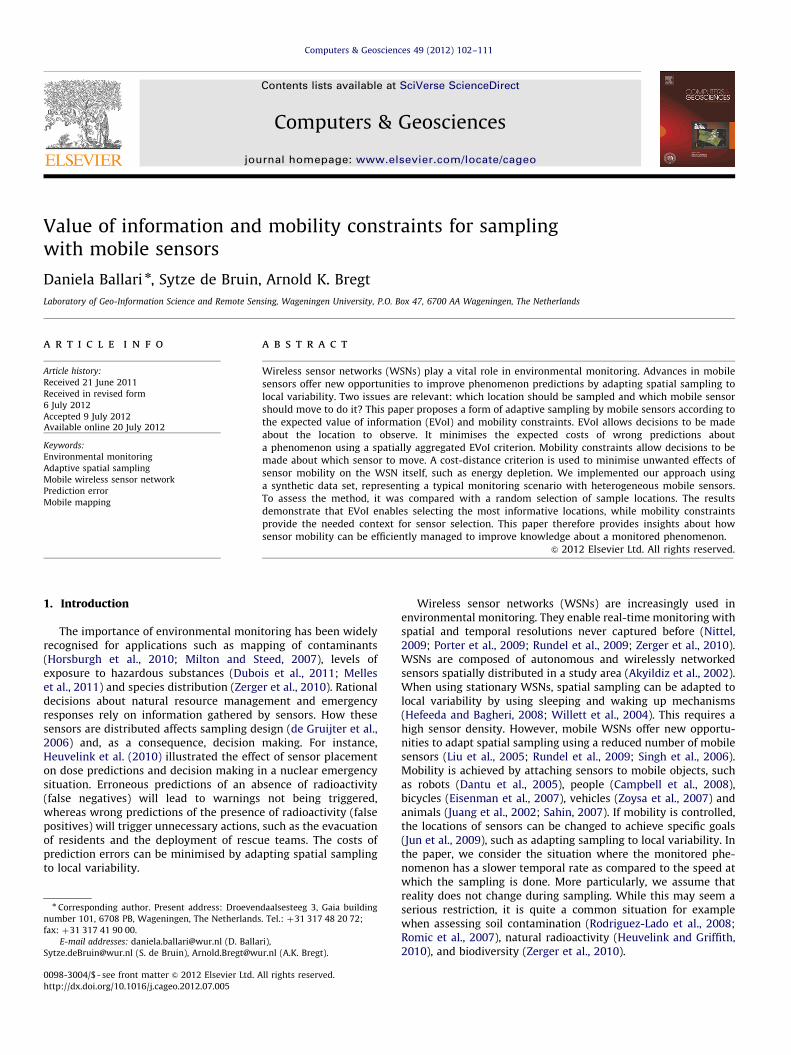
Fig. 1. Decision tree for sampling a location: (a) prior expected cost of wrong

predictions and (b) posterior expected cost of wrong predictions. Squares are

decision nodes; circles are chance nodes. The grey column shows the misclassi-

fication costs assigned to each leaf of the decision tree.

Decide to sample atalocation or not

C (T,F)Phenomenon

presence

Additionalobservation

Decide state of F

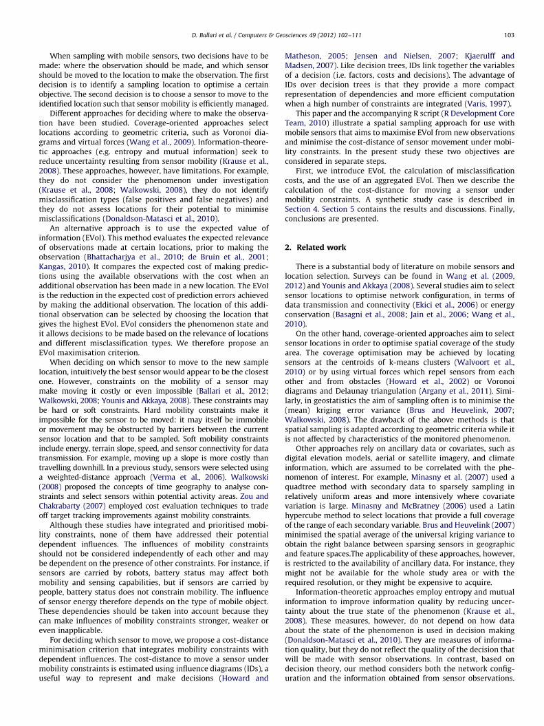
Fig. 2. Influence diagram representing the decision tree in Fig. 1.

3. Methods

3.1. Value of information

The expected value of information (EVoI) is the differencebetween the prior and posterior costs of wrong predictions:

EVoI¼ E Cprior

� ��E Cposterior

� �ð1Þ

Consider a WSN with mobile sensors deployed in a study area.Sensors monitor at locations (L) a certain phenomenon (F) which,for simplicity, has either of two states (T): presence or absence.Prior information about the phenomenon is given by a set ofdiscrete observations made by the sensors. These observations areinterpolated to predict, at unobserved locations, the probability ofthe phenomenon being present P(f¼present). This is called theprior probability map.

Using the prior probability map, unobserved locations arelabelled as ‘phenomenon present’ or ‘phenomenon absent’. Tominimise misclassification costs, Bayes decision principle choosesthe state with the minimum expected cost (Eq. (2)) (Berger,1985). Let C(T,F) be the misclassification costs: Cwrong-p for wrongpredictions of phenomenon present, and Cwrong-a for wrong pre-dictions of phenomenon absent. There are no costs for correctpredictions. The expected cost is based on available observations,thus it is called the prior expected cost of wrong predictions.Fig. 1a illustrates this decision as a decision tree.

E Cprior

� �¼min C T ,Fð ÞP Flð Þð Þ ð2Þ

As the EVoI is evaluated before moving a sensor, Bayes theoremis used to update the prior probability P(F) into a posteriorprobability P(F9X), where X represents the new data. Because Xhas not been observed yet, the posterior probability P(F9X) iscalculated from all possible outcomes of X (signals of presence andabsence) and for all possible locations in the study area. In Eq. (3),P(F) is the prior probability obtained using available observationsat a considered location. P(X9F) is the likelihood of getting apresence signal if the phenomenon is actually present. Informationabout P(X9F) can be obtained from sensor sensitivity and specifi-city data in the sensor specifications. P(X) is the probability ofgetting a presence signal at the considered location. It is obtainedby marginalising out the likelihood P(X9F) over the possible statesof F. In case of no measurement errors P(X) equals P(F):

P Fl9Xl

� �¼ P X9F� �

P Flð Þ=P Xlð Þ;

P Xlð Þ ¼X

F

P X9F� �

P Flð Þ ð3Þ

The posterior expected cost is calculated as in Eq. (2), but usingthe posterior probability P(F9X) for all the possible outcomesof X (Eq. (4)). Following Bayes decision principle, the minimumexpected costs of each outcome is weighted with P(X). This cost iscalculated after updating the prior probability into a posterior

one, thus it is called the posterior cost of wrong predictions.Fig. 1b illustrates this decision as a decision tree. Fig. 2 is aninfluence diagram for the decision tree shown in Fig. 1.

E Cposterior

� �¼X

X

P Xlð Þmin C T ,Fð ÞP Fl9Xl

� �� �ð4Þ

Finally, EVoI is calculated for each unobserved location usingEq. (1). If E(Cposterior) is smaller than E(Cprior), information has beengained and the misclassification cost reduced.

3.2. Aggregated EVoI

The EVoI calculated as described above is called the ‘localEVoI’. However, spatial correlation between observations meansthat an observation carries information not only about its ownlocation, but also about its vicinity. The expected reduction inmisclassification costs aggregated over the whole study area isthe ‘aggregated EVoI’. Maximising aggregated EVoI is equivalentto minimising misclassification costs over the whole study area.

Aggregated EVoI is calculated as the difference between theprior and posterior costs which have been aggregated over thewhole map. A posterior probability map is predicted (interpo-lated) for each possible outcome of X and for each unobservedlocation. Then, for each posterior probability map, the posteriorexpected cost is calculated using Eq. (4), and aggregated over thewhole map. The location with the maximum aggregated EVoI isselected to be sampled.

D. Ballari et al. / Computers & Geosciences 49 (2012) 102–111 105

3.3. Mobility constraints

The next step is to decide which sensor to move to the newlocation by calculating the cost-distances of moving each sensor.The sensor with the lowest cost-distance is selected.

We use influence diagrams (IDs) to integrate the mobilityconstraints into the calculation of cost-distances. An ID graphi-cally represents the decision problem including the decision,factors and costs (Howard and Matheson, 2005; Jensen andNielsen, 2007; Kjaerulff and Madsen, 2007).

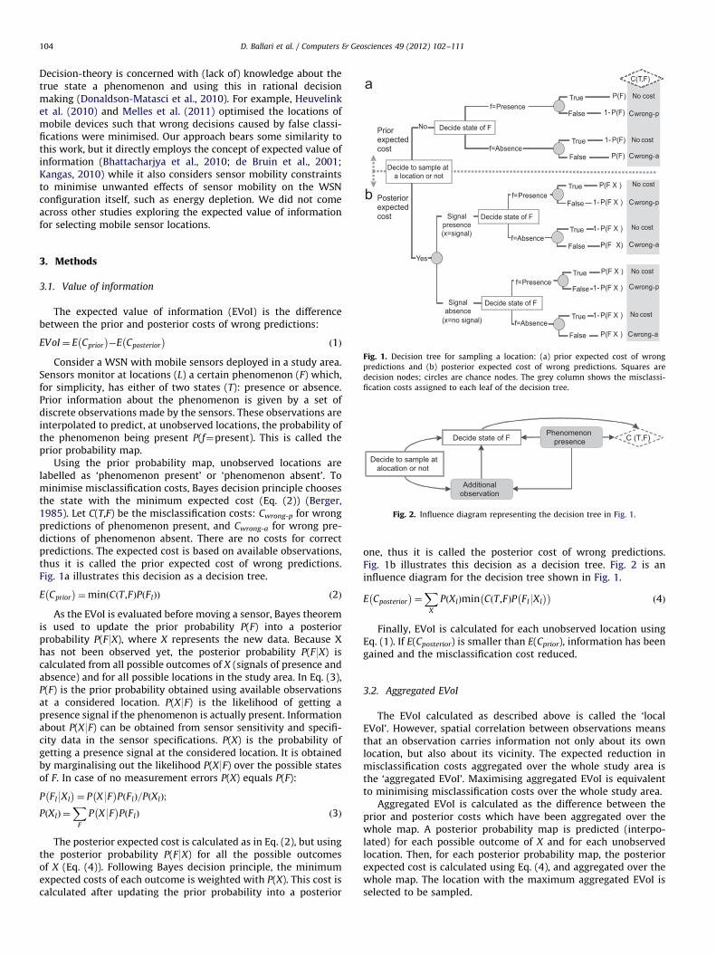
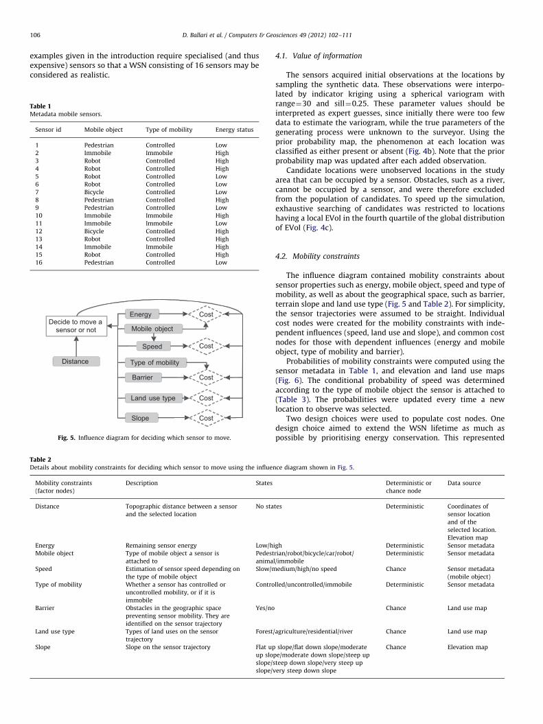
The decision is whether to move a sensor or not. Factors aremobility constraints (MC) represented by sensor properties (i.e.energy, type of mobility, mobile object, speed, connectivity, etc.),a selected sensor trajectory and properties of the geographicalspace (i.e. barriers, slope, type of land use, etc.). Distance is alsoconsidered as a factor and depends on the selected sensortrajectory. Costs are the decision maker’s preferences for eachdecision alternative, given the possible states of mobility con-straints. Fig. 3 shows the influence diagram with the decision as asquare, factors as grey rounded squares, and the cost node asa diamond. The arrows pointing to the decision node are informa-tional and represent the known information at the time of makingthe decision. The arrows pointing to the cost node are functionaland represent the link between cost values and the underlyingmobility constraints and the decision.

The cost-distance of moving a sensor (s) under mobilityconstraints is calculated using Eq. (5), in which (d¼move) is thedecision to move the sensor. The cost values (C(d¼move, MC)) aremultiplied by the probability of mobility constraints being pre-sent (P(MC)) and the distance to travel (dist).

Cost-distances ¼ dists C d¼move,MCsð ÞP MCsð Þð Þ ð5Þ

As it may be difficult to assess cost values in an integratedway when several mobility constraints are considered, costs arebroken down by mobility constraints. However, the cost values of

Decide to move asensor or not C (D,MC)

Mobility constraintsSensor propertiesSensor trajectory

Geographical space

Distance

Fig. 3. General influence diagram for deciding which sensor to move.

(a) Phenomenon presencePhenomenon absence

Predicted phenomenon Predicted phenomenon

(b)

Legend

2 Deployed sensors

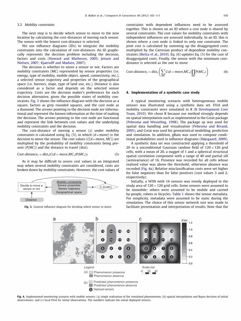
Fig. 4. Implemented monitoring scenario with mobile sensors: (a) single realisation of

observations; and (c) local EVoI for initial observations. The numbers indicate the initi

constraints with dependent influences need to be assessedtogether. This is shown on an ID where a cost node is shared byseveral constraints. The cost values for mobility constraints withindependent influences are assessed individually. In an ID, this isshown where a cost node is linked to only one constraint. Thejoint cost is calculated by summing up the disaggregated costsmultiplied by the Cartesian product of dependent mobility con-straints (Bielza et al., 2010). Eq. (6) updates Eq. (5) for the case ofdisaggregated costs. Finally, the sensor with the minimum cost-distance is selected as the one to move

Cost-distances ¼ dists

XMC

C d¼move,MCsð ÞYMC

P MCsð Þ

!ð6Þ

4. Implementation of a synthetic case study

A typical monitoring scenario with heterogeneous mobilesensors was illustrated using a synthetic data set. EVoI andmobility constraints were simulated in R (R Development CoreTeam, 2010). We chose R because our method strongly dependson spatial interpolation such as implemented in the Gstat package(Pebesma and Wesseling, 1998). The package sp was used forspatial data handling and visualisation (Pebesma and Bivand,2005), and Gstat was used for geostatistical modelling, predictionand simulation. In addition, gRain was used to compute condi-tional probabilities used in influence diagrams (Højsgaard, 2009).

A synthetic data set was constructed applying a threshold of20 to a unconditional Gaussian random field of 120�120 gridcells, with a mean of 20, a nugget of 1 and a spherical structuralspatial correlation component with a range of 40 and partial sill(semivariance) of 16. Presence was recorded for all cells whoserealised value was above the threshold; otherwise absence wasrecorded (Fig. 4a). Relative misclassification costs were set higherfor false negatives than for false positives (cost values 3 and 2,respectively).

Initially, a WSN with 16 sensors was evenly deployed in thestudy area of 120�120 grid cells. Some sensors were assumed tobe immobile; others were assumed to be mobile and carriedby people, robots or bicycles. Table 1 shows the sensor metadata.For simplicity, metadata were assumed to be static during thesimulation. The choice of this sensor network size was made tofacilitate presentation and interpretation of results. Note that the

m 40

presenceabsence

Scale bar20

the simulated phenomenon; (b) spatial interpolation and Bayes decision of initial

al deployed sensors.

D. Ballari et al. / Computers & Geosciences 49 (2012) 102–111106

examples given in the introduction require specialised (and thusexpensive) sensors so that a WSN consisting of 16 sensors may beconsidered as realistic.

Table 1Metadata mobile sensors.

Sensor id Mobile object Type of mobility Energy status

1 Pedestrian Controlled Low

2 Immobile Immobile High

3 Robot Controlled High

4 Robot Controlled High

5 Robot Controlled Low

6 Robot Controlled Low

7 Bicycle Controlled Low

8 Pedestrian Controlled High

9 Pedestrian Controlled Low

10 Immobile Immobile High

11 Immobile Immobile Low

12 Bicycle Controlled High

13 Robot Controlled High

14 Immobile Immobile High

15 Robot Controlled High

16 Pedestrian Controlled Low

Energy

Type of mobility

Mobile object

Speed

Barrier

Land use type

Slope

Cost

Cost

Cost

Cost

Cost

Decide to move asensor or not

Distance

Fig. 5. Influence diagram for deciding which sensor to move.

Table 2Details about mobility constraints for deciding which sensor to move using the influen

Mobility constraints

(factor nodes)

Description States

Distance Topographic distance between a sensor

and the selected location

No sta

Energy Remaining sensor energy Low/h

Mobile object Type of mobile object a sensor is

attached to

Pedest

anima

Speed Estimation of sensor speed depending on

the type of mobile object

Slow/m

Type of mobility Whether a sensor has controlled or

uncontrolled mobility, or if it is

immobile

Contro

Barrier Obstacles in the geographic space

preventing sensor mobility. They are

identified on the sensor trajectory

Yes/no

Land use type Types of land uses on the sensor

trajectory

Forest/

Slope Slope on the sensor trajectory Flat up

up slo

slope/s

slope/v

4.1. Value of information

The sensors acquired initial observations at the locations bysampling the synthetic data. These observations were interpo-lated by indicator kriging using a spherical variogram withrange¼30 and sill¼0.25. These parameter values should beinterpreted as expert guesses, since initially there were too fewdata to estimate the variogram, while the true parameters of thegenerating process were unknown to the surveyor. Using theprior probability map, the phenomenon at each location wasclassified as either present or absent (Fig. 4b). Note that the priorprobability map was updated after each added observation.

Candidate locations were unobserved locations in the studyarea that can be occupied by a sensor. Obstacles, such as a river,cannot be occupied by a sensor, and were therefore excludedfrom the population of candidates. To speed up the simulation,exhaustive searching of candidates was restricted to locationshaving a local EVoI in the fourth quartile of the global distributionof EVoI (Fig. 4c).

4.2. Mobility constraints

The influence diagram contained mobility constraints aboutsensor properties such as energy, mobile object, speed and type ofmobility, as well as about the geographical space, such as barrier,terrain slope and land use type (Fig. 5 and Table 2). For simplicity,the sensor trajectories were assumed to be straight. Individualcost nodes were created for the mobility constraints with inde-pendent influences (speed, land use and slope), and common costnodes for those with dependent influences (energy and mobileobject, type of mobility and barrier).

Probabilities of mobility constraints were computed using thesensor metadata in Table 1, and elevation and land use maps(Fig. 6). The conditional probability of speed was determinedaccording to the type of mobile object the sensor is attached to(Table 3). The probabilities were updated every time a newlocation to observe was selected.

Two design choices were used to populate cost nodes. Onedesign choice aimed to extend the WSN lifetime as much aspossible by prioritising energy conservation. This represented

ce diagram shown in Fig. 5.

Deterministic or

chance node

Data source

tes Deterministic Coordinates of

sensor location

and of the

selected location.

Elevation map

igh Deterministic Sensor metadata

rian/robot/bicycle/car/robot/

l/immobile

Deterministic Sensor metadata

edium/high/no speed Chance Sensor metadata

(mobile object)

lled/uncontrolled/immobile Deterministic Sensor metadata

Chance Land use map

agriculture/residential/river Chance Land use map

slope/flat down slope/moderate

pe/moderate down slope/steep up

teep down slope/very steep up

ery steep down slope

Chance Elevation map

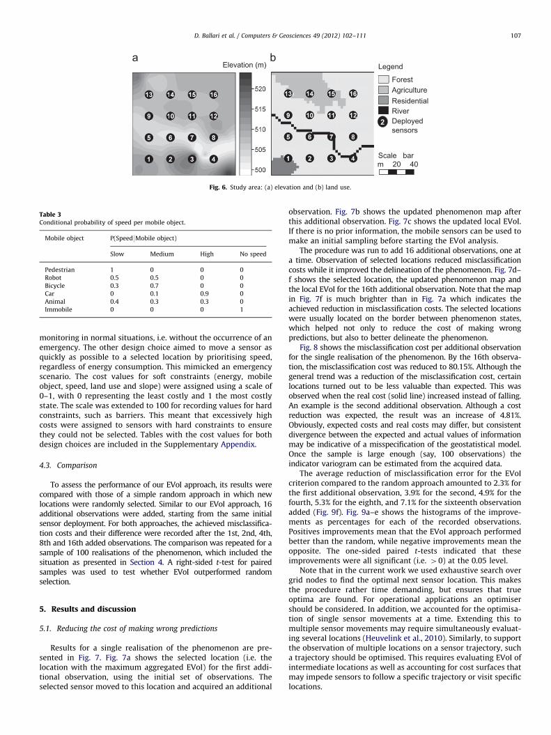
ForestAgricultureResidentialRiver

m 40

Legend

2 Deployedsensors

Scale bar20

Elevation (m)

Fig. 6. Study area: (a) elevation and (b) land use.

Table 3Conditional probability of speed per mobile object.

Mobile object P(Speed9Mobile object)

Slow Medium High No speed

Pedestrian 1 0 0 0

Robot 0.5 0.5 0 0

Bicycle 0.3 0.7 0 0

Car 0 0.1 0.9 0

Animal 0.4 0.3 0.3 0

Immobile 0 0 0 1

D. Ballari et al. / Computers & Geosciences 49 (2012) 102–111 107

monitoring in normal situations, i.e. without the occurrence of anemergency. The other design choice aimed to move a sensor asquickly as possible to a selected location by prioritising speed,regardless of energy consumption. This mimicked an emergencyscenario. The cost values for soft constraints (energy, mobileobject, speed, land use and slope) were assigned using a scale of0–1, with 0 representing the least costly and 1 the most costlystate. The scale was extended to 100 for recording values for hardconstraints, such as barriers. This meant that excessively highcosts were assigned to sensors with hard constraints to ensurethey could not be selected. Tables with the cost values for bothdesign choices are included in the Supplementary Appendix.

4.3. Comparison

To assess the performance of our EVoI approach, its results werecompared with those of a simple random approach in which newlocations were randomly selected. Similar to our EVoI approach, 16additional observations were added, starting from the same initialsensor deployment. For both approaches, the achieved misclassifica-tion costs and their difference were recorded after the 1st, 2nd, 4th,8th and 16th added observations. The comparison was repeated for asample of 100 realisations of the phenomenon, which included thesituation as presented in Section 4. A right-sided t-test for pairedsamples was used to test whether EVoI outperformed randomselection.

5. Results and discussion

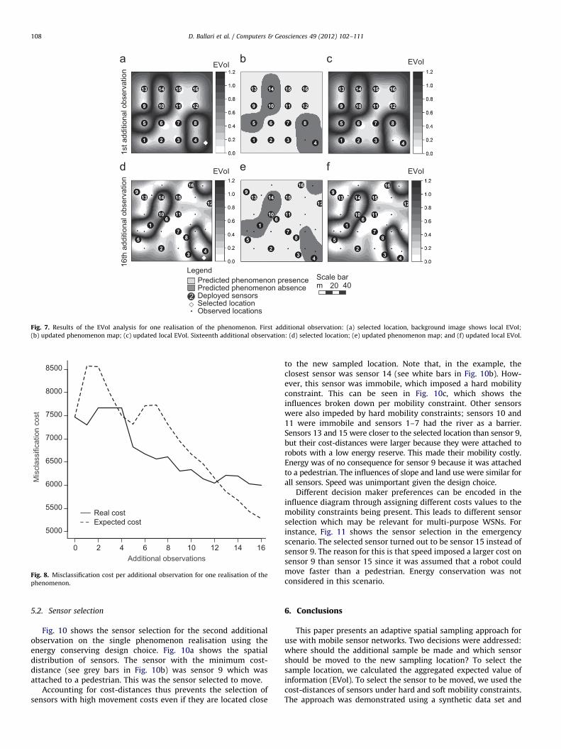
5.1. Reducing the cost of making wrong predictions

Results for a single realisation of the phenomenon are pre-sented in Fig. 7. Fig. 7a shows the selected location (i.e. thelocation with the maximum aggregated EVoI) for the first addi-tional observation, using the initial set of observations. Theselected sensor moved to this location and acquired an additional

observation. Fig. 7b shows the updated phenomenon map afterthis additional observation. Fig. 7c shows the updated local EVoI.If there is no prior information, the mobile sensors can be used tomake an initial sampling before starting the EVoI analysis.

The procedure was run to add 16 additional observations, one ata time. Observation of selected locations reduced misclassificationcosts while it improved the delineation of the phenomenon. Fig. 7d–f shows the selected location, the updated phenomenon map andthe local EVoI for the 16th additional observation. Note that the mapin Fig. 7f is much brighter than in Fig. 7a which indicates theachieved reduction in misclassification costs. The selected locationswere usually located on the border between phenomenon states,which helped not only to reduce the cost of making wrongpredictions, but also to better delineate the phenomenon.

Fig. 8 shows the misclassification cost per additional observationfor the single realisation of the phenomenon. By the 16th observa-tion, the misclassification cost was reduced to 80.15%. Although thegeneral trend was a reduction of the misclassification cost, certainlocations turned out to be less valuable than expected. This wasobserved when the real cost (solid line) increased instead of falling.An example is the second additional observation. Although a costreduction was expected, the result was an increase of 4.81%.Obviously, expected costs and real costs may differ, but consistentdivergence between the expected and actual values of informationmay be indicative of a misspecification of the geostatistical model.Once the sample is large enough (say, 100 observations) theindicator variogram can be estimated from the acquired data.

The average reduction of misclassification error for the EVoIcriterion compared to the random approach amounted to 2.3% forthe first additional observation, 3.9% for the second, 4.9% for thefourth, 5.3% for the eighth, and 7.1% for the sixteenth observationadded (Fig. 9f). Fig. 9a–e shows the histograms of the improve-ments as percentages for each of the recorded observations.Positives improvements mean that the EVoI approach performedbetter than the random, while negative improvements mean theopposite. The one-sided paired t-tests indicated that theseimprovements were all significant (i.e. 40) at the 0.05 level.

Note that in the current work we used exhaustive search overgrid nodes to find the optimal next sensor location. This makesthe procedure rather time demanding, but ensures that trueoptima are found. For operational applications an optimisershould be considered. In addition, we accounted for the optimisa-tion of single sensor movements at a time. Extending this tomultiple sensor movements may require simultaneously evaluat-ing several locations (Heuvelink et al., 2010). Similarly, to supportthe observation of multiple locations on a sensor trajectory, sucha trajectory should be optimised. This requires evaluating EVoI ofintermediate locations as well as accounting for cost surfaces thatmay impede sensors to follow a specific trajectory or visit specificlocations.

1st a

dditi

onal

obs

erva

tion

16th

add

ition

al o

bser

vatio

n

Selected locationObserved locations

m 40Predicted phenomenon presencePredicted phenomenon absence

Legend

2 Deployed sensors

Scale bar20

EVoIEVoI

EVoIEVoI

Fig. 7. Results of the EVoI analysis for one realisation of the phenomenon. First additional observation: (a) selected location, background image shows local EVoI;

(b) updated phenomenon map; (c) updated local EVoI. Sixteenth additional observation: (d) selected location; (e) updated phenomenon map; and (f) updated local EVoI.

5000

5500

6000

6500

7000

7500

8000

8500

0 10 12 14 16

Real costExpected cost

Additional observations

Mis

clas

sific

atio

n co

st

2 4 6 8

Fig. 8. Misclassification cost per additional observation for one realisation of the

phenomenon.

D. Ballari et al. / Computers & Geosciences 49 (2012) 102–111108

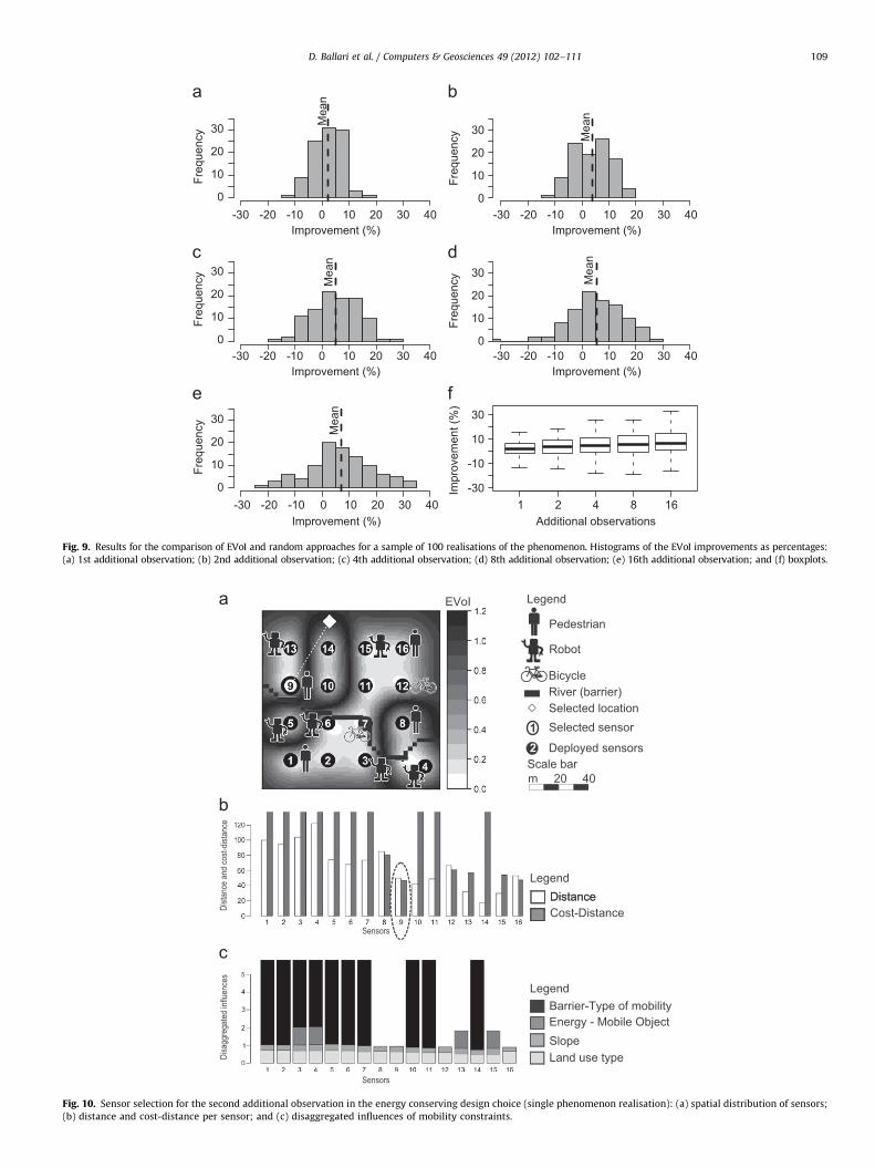
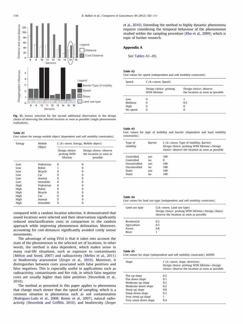
5.2. Sensor selection

Fig. 10 shows the sensor selection for the second additionalobservation on the single phenomenon realisation using theenergy conserving design choice. Fig. 10a shows the spatialdistribution of sensors. The sensor with the minimum cost-distance (see grey bars in Fig. 10b) was sensor 9 which wasattached to a pedestrian. This was the sensor selected to move.

Accounting for cost-distances thus prevents the selection ofsensors with high movement costs even if they are located close

to the new sampled location. Note that, in the example, theclosest sensor was sensor 14 (see white bars in Fig. 10b). How-ever, this sensor was immobile, which imposed a hard mobilityconstraint. This can be seen in Fig. 10c, which shows theinfluences broken down per mobility constraint. Other sensorswere also impeded by hard mobility constraints; sensors 10 and11 were immobile and sensors 1–7 had the river as a barrier.Sensors 13 and 15 were closer to the selected location than sensor 9,but their cost-distances were larger because they were attached torobots with a low energy reserve. This made their mobility costly.Energy was of no consequence for sensor 9 because it was attachedto a pedestrian. The influences of slope and land use were similar forall sensors. Speed was unimportant given the design choice.

Different decision maker preferences can be encoded in theinfluence diagram through assigning different costs values to themobility constraints being present. This leads to different sensorselection which may be relevant for multi-purpose WSNs. Forinstance, Fig. 11 shows the sensor selection in the emergencyscenario. The selected sensor turned out to be sensor 15 instead ofsensor 9. The reason for this is that speed imposed a larger cost onsensor 9 than sensor 15 since it was assumed that a robot couldmove faster than a pedestrian. Energy conservation was notconsidered in this scenario.

6. Conclusions

This paper presents an adaptive spatial sampling approach foruse with mobile sensor networks. Two decisions were addressed:where should the additional sample be made and which sensorshould be moved to the new sampling location? To select thesample location, we calculated the aggregated expected value ofinformation (EVoI). To select the sensor to be moved, we used thecost-distances of sensors under hard and soft mobility constraints.The approach was demonstrated using a synthetic data set and

-30 -20 -10 10 20 30 40Fr

eque

ncy

-30 -20 -10 10 20 30 40 1 2 16

Impr

ovem

ent (

%)

Mea

n

Mea

n

Mea

n

Mea

n

Mea

n

0

10

20

30

Freq

uenc

y

0

10

20

30

Freq

uenc

y

0

10

20

30

Freq

uenc

y

0

10

20

30

Freq

uenc

y

0

10

20

30

0Improvement (%)

-30 -20 -10 10 20 30 400Improvement (%)

-30 -20 -10 10 20 30 400Improvement (%)

-30 -20 -10 10 20 30 400Improvement (%)

30

10

-10

-30

Additional observations4 80

Improvement (%)

Fig. 9. Results for the comparison of EVoI and random approaches for a sample of 100 realisations of the phenomenon. Histograms of the EVoI improvements as percentages:

(a) 1st additional observation; (b) 2nd additional observation; (c) 4th additional observation; (d) 8th additional observation; (e) 16th additional observation; and (f) boxplots.

Distance

Land use typeSlope

Barrier-Type of mobility

Pedestrian

Robot

Dista

nce

and

cost-

dista

nce

River (barrier)

12

Selected locationSelected sensor

Deployed sensors

Energy - Mobile Object

DistanceCost-Distance

Disa

ggre

gate

d inf

luenc

es

Sensors

Sensors

Bicycle

EVoI Legend

Legend

Legend

m 40Scale bar

20

Fig. 10. Sensor selection for the second additional observation in the energy conserving design choice (single phenomenon realisation): (a) spatial distribution of sensors;

(b) distance and cost-distance per sensor; and (c) disaggregated influences of mobility constraints.

D. Ballari et al. / Computers & Geosciences 49 (2012) 102–111 109

Land use type

Slope

Barrier-Type of mobility

Dis

tanc

e an

d co

st-d

ista

nce

Speed

Distance

Dis

aggr

egat

ed in

fluen

ces

Legend

Legend

Sensors

Sensors

Cost-Distance

Fig. 11. Sensor selection for the second additional observation in the design

choice of observing the selected location as soon as possible (single phenomenon

realisation).

Table A1Cost values for energy-mobile object (dependent and soft mobility constraints).

Energy Mobile

Object

C (d¼move, Energy, Mobile object)

Design choice:

prolong WSN

lifetime

Design choice: observe

the location as soon as

possible

Low Pedestrian 0 0

Low Robot 1 0

Low Bicycle 0 0

Low Car 0 0

Low Animal 0 0

Low Immobile 0 0

High Pedestrian 0 0

High Robot 0 0

High Bicycle 0 0

High Car 0 0

High Animal 0 0

High Immobile 0 0

Table A2Cost values for speed (independent and soft mobility constraint).

Speed C (d¼move, Speed)

Design choice: prolong

WSN lifetime

Design choice: observe

the location as soon as possible

Low 0 1

Medium 0 0.5

High 0 0

No speed 0 0

Table A3Cost values for type of mobility and barrier (dependent and hard mobility

constraints).

Type of

mobility

Barrier C (d¼move, Type of mobility, Barrier)

Design choice: prolong WSN lifetime¼Design

choice: observe the location as soon as possible

Controlled yes 100

Controlled no 0

Uncontrolled yes 100

Uncontrolled no 100

Static yes 100

Static no 100

Table A4Cost values for land use type (independent and soft mobility constraint).

Land use type C(d¼move, Land use type)

Design choice: prolong WSN lifetime¼Design choice:

observe the location as soon as possible

Residential 0.2

Agriculture 0.5

Forest 0.8

River 1

Table A5Cost values for slope (independent and soft mobility constraint). ADDIN

Slope C (d¼move, slope, direction)

Design choice: prolong WSN lifetime¼Design

choice: observe the location as soon as possible

Flat up slope 0.2

Flat down slope 0.1

Moderate up slope 0.5

Moderate down slope 0.2

Steep up slope 0.8

Steep down slope 0.3

Very steep up slope 1

Very steep down slope 0.4

D. Ballari et al. / Computers & Geosciences 49 (2012) 102–111110

compared with a random location selection. It demonstrated thatsound locations were selected and their observations significantlyreduced misclassification costs in comparison to the randomapproach while improving phenomenon delineation. Moreover,accounting for cost-distances significantly avoided costly sensormovements.

The advantage of using EVoI is that it takes into account thestate of the phenomenon in the selected set of locations. In otherwords, the method is data dependent, which makes sense inmany real-life situations, such as exposure to contaminants(Milton and Steed, 2007) and radioactivity (Melles et al., 2011)or biodiversity assessment (Zerger et al., 2010). Moreover, itdistinguishes between costs associated with false positives andfalse negatives. This is especially useful in applications such asradioactivity, contaminants and fire risk, in which false negativecosts are usually higher than false positives (Heuvelink et al.,2010).

The method as presented in this paper applies to phenomenathat change much slower than the speed of sampling, which is acommon situation in phenomena such as soil contamination(Rodriguez-Lado et al., 2008; Romic et al., 2007), natural radio-activity (Heuvelink and Griffith, 2010), and biodiversity (Zerger

et al., 2010). Extending the method to highly dynamic phenomenarequires considering the temporal behaviour of the phenomenonstudied within the sampling procedure (Kho et al., 2009), which istopic of further research.

Appendix A

See Tables A1–A5.

D. Ballari et al. / Computers & Geosciences 49 (2012) 102–111 111

Appendix A. Supplementary material

Supplementary data associated with this article can be found inthe online version at http://dx.doi.org/10.1016/j.cageo.2012.07.005.

References

Akyildiz, I., Su, W., Sankarasubramaniam, Y., Cayirci, E., 2002. Wireless sensornetworks: a survey. Computer Networks 38, 393–422.

Argany, M., Mostafavi, M., Karimipour, F., Gagne, C., 2011. A GIS based wirelesssensor network coverage estimation and optimization: a Voronoi approach.Transactions on Computational Science XIV, 151–172.

Ballari, D., Wachowicz, M., Bregt, A.K., Manso-Callejo, M., 2012. A mobilityconstraint model to infer sensor behaviour in forest fire risk monitoring.Computers, Environment and Urban Systems 36, 81–95.

Basagni, S., Carosi, A., Melachrinoudis, E., Petrioli, C., Wang, Z., 2008. Controlledsink mobility for prolonging wireless sensor networks lifetime. WirelessNetworks 14, 831–858.

Berger, J.O., 1985. Statistical Decision Theory and Bayesian Analysis. Springer.Bhattacharjya, D., Eidsvik, J., Mukerji, T., 2010. The value of information in spatial

decision making. Mathematical Geosciences 42, 141–163.Bielza, C., Gomez, M., Shenoy, P.P., 2010. Modeling challenges with influence

diagrams: constructing probability and utility models. Decision SupportSystems 49, 354–364.

Brus, D.J., Heuvelink, G., 2007. Optimization of sample patterns for universalkriging of environmental variables. Geoderma 138, 86–95.

Campbell, A., Eisenman, S., Lane, N., Miluzzo, E., Peterson, R., Lu, H., Zheng, X.,Musolesi, M., Fodor, K., Ahn, G., 2008. The rise of people-centric sensing. IEEEInternet Computing 4, 12–21.

Dantu, K., Rahimi, M., Shah, H., Babel, S., Dhariwal, A., Sukhatme, G.S., 2005.Robomote: enabling mobility in sensor networks. In: Proceedings of the 4thInternational Symposium on Information Processing in Sensor Networks. IEEEPress, Los Angeles, California, USA, pp. 404–409.

de Bruin, S., Bregt, A., van de Ven, M., 2001. Assessing fitness for use: the expectedvalue of spatial data sets. International Journal of Geographical InformationScience 15, 457–471.

de Gruijter, J., Brus, D.J., Bierkens, M.F.P., Knotters, M., 2006. Sampling for NaturalResource Monitoring, 1st edn. Springer Verlag, Berlin, Heidelberg, New York332 pp.

Donaldson-Matasci, M.C., Bergstrom, C.T., Lachmann, M., 2010. The fitness value ofinformation. Oikos 119, 219–230.

Dubois, G., Cornford, D., Hristopulos, D., Pebesma, E., Pilz, J., 2011. Introduction tothis special issue on geoinformatics for environmental surveillance. Compu-ters & Geosciences 37, 277–279.

Eisenman, S., Miluzzo, E., Lane, N., Peterson, R., Ahn, G., Campbell, A., 2007. TheBikeNet mobile sensing system for cyclist experience mapping. In: Proceedingsof the 5th Conference on Embedded Networked Sensor Systems, pp. 87–101.

Ekici, E., Gu, Y., Bozdag, D., 2006. Mobility-based communication in wirelesssensor networks. IEEE Communications Magazine 44, 56–62.

Hefeeda, M., Bagheri, M., 2008. Forest fire modeling and early detection usingwireless sensor networks. Ad Hoc & Sensor Wireless Networks 7, 169–224.

Heuvelink, G., Griffith, D.A., 2010. Space–time geostatistics for geography: a casestudy of radiation monitoring across parts of Germany. Geographical Analysis42, 161–179.

Heuvelink, G., Jiang, Z., De Bruin, S., Twenhofel, C., 2010. Optimization of mobileradioactivity monitoring networks. International Journal of GeographicalInformation Science 24, 365–382.

Højsgaard, S., 2009. gRain; A Graphical Independence Networks package in R.Horsburgh, J.S., Spackman Jones, A., Stevens, D.K., Tarboton, D.G., Mesner, N.O.,

2010. A sensor network for high frequency estimation of water qualityconstituent fluxes using surrogates. Environmental Modelling & Software 25,1031–1044.

Howard, A., Mataric, M.J., Sukhatme, G.S., 2002. Mobile sensor network deploy-ment using potential fields: a distributed, scalable solution to the areacoverage problem. In: Proceedings of the 6th International Symposium onDistributed Autonomous Robotics Systems (DARS02). Citeseer, pp. 299–308.

Howard, R.A., Matheson, J.E., 2005. Influence diagrams. Decision Analysis 2,127–143.

Jain, S., Shah, R., Brunette, W., Borriello, G., Roy, S., 2006. Exploiting mobility forenergy efficient data collection in wireless sensor networks. Mobile Networksand Applications 11, 327–339.

Jensen, F., Nielsen, T., 2007. Bayesian Networks and Decision Graphs, 2nd edn.Springer, Berlin.

Juang, P., Oki, H., Wang, Y., Martonosi, M., Peh, L., Rubenstein, D., 2002. Energy-efficient computing for wildlife tracking: design tradeoffs and early experi-ences with zebranet, SIGOPS operating systems review. In: Proceedings of the10th annual conference on Architectural Support for Programming Languagesand Operating Systems, pp. 96–107.

Jun, J., Xie, B., Agrawal, D., 2009. Wireless mobile sensor networks: protocols andmobility strategies. In: Misra, S.C., Woungang, I., Misra, S., Jun, J.H., Xie, B.,

Agrawal, D.P. (Eds.), Guide to Wireless Sensor Networks. Springer, London,pp. 611–638.

Kangas, A., 2010. Value of forest information. European Journal of Forest Research129, 863–874.

Kho, J., Rogers, A., Jennings, N.R., 2009. Decentralized control of adaptive sampling inwireless sensor networks. ACM Transactions on Sensor Networks (TOSN) 5, 19.

Kjaerulff, U.B., Madsen, A.L., 2007. Bayesian Networks and Influence Diagrams: AGuide to Construction and Analysis. Springer Verlag.

Krause, A., Singh, A., Guestrin, C., 2008. Near-optimal sensor placements inGaussian processes: theory, efficient algorithms and empirical studies. Journalof Machine Learning Research 9, 235–284.

Liu, B., Brass, P., Dousse, O., Nain, P., Towsley, D., 2005. Mobility improves coverage ofsensor networks. In: Proceedings of the 6th international symposium on mobilead hoc networking and computing, Urbana-Champaign, USA. pp. 300–308.

Melles, S.J., Heuvelink, G.B.M., Twenhofel, C.J.W., van Dijk, A., Hiemstra, P.H.,Baume, O., Stohlker, U., 2011. Optimizing the spatial pattern of networks formonitoring radioactive releases. Computers & Geosciences 37, 280–288.

Milton, R., Steed, A., 2007. Mapping carbon monoxide using GPS tracked sensors.Environmental monitoring and Assessment 124, 1–19.

Minasny, B., McBratney, A.B., 2006. A conditioned Latin hypercube method forsampling in the presence of ancillary information. Computers & Geosciences32, 1378–1388.

Minasny, B., McBratney, A.B., Walvoort, D.J.J., 2007. The variance quadtreealgorithm: use for spatial sampling design. Computers & Geosciences 33,383–392.

Nittel, S., 2009. A survey of geosensor networks: advances in dynamic environ-mental monitoring. Sensors 9, 5664–5678.

Pebesma, E.J., Bivand, R.S., 2005. Classes and methods for spatial data in R. R News5, 9–13.

Pebesma, E.J., Wesseling, C.G., 1998. Gstat: a program for geostatistical modelling,prediction and simulation. Computers & Geosciences 24, 17–31.

Porter, J., Nagy, E., Kratz, T., Hanson, P., Collins, S., Arzberger, P., 2009. New eyes onthe world: advanced sensors for ecology. BioScience 59, 385–397.

R Development Core Team, 2010. R: A Language and Environment for StatisticalComputing. R Foundation for Statistical Computing, Vienna, Austria. ISBN3-900051-07-0, /http://www.R-project.orgS.

Rodriguez-Lado, L., Hengl, T., Reuter, H.I., 2008. Heavy metals in European soils: ageostatistical analysis of the FOREGS geochemical database. Geoderma 148,189–199.

Romic, M., Hengl, T., Romic, D., Husnjak, S., 2007. Representing soil pollution byheavy metals using continuous limitation scores. Computers & Geosciences 33,1316–1326.

Rundel, P.W., Graham, E.A., Allen, M.F., Fisher, J.C., Harmon, T.C., 2009. Environ-mental sensor networks in ecological research. New Phytologist 182, 589–607.

Sahin, Y., 2007. Animals as mobile biological sensors for forest fire detection.Sensors 7, 3084–3099.

Singh, A., Budzik, D., Chen, W., Batalin, M., Kaiser, W., 2006. Multiscale sensing: anew paradigm for actuated sensing of high frequency dynamic phenomena. In:Proceedings of the IEEE/RSJ International Conference on Intelligent Robots andSystems, Beijing, pp. 328–335.

Varis, O., 1997. Bayesian decision analysis for environmental and resourcemanagement. Environmental Modelling & Software 12, 177–185.

Verma, A., Sawant, H., Tan, J., 2006. Selection and navigation of mobile sensornodes using a sensor network. Pervasive and Mobile Computing 2, 65–84.

Walkowski, A.C., 2008. Model based optimization of mobile geosensor networks.In: Bernard, L., Friis-Christensen, A., Pundt, H. (Eds.), The European InformationSociety. Springer, Berlin Heidelberg, pp. 51–66.

Walvoort, D., Brus, D., de Gruijter, J., 2010. An R package for spatial coveragesampling and random sampling from compact geographical strata by k-means.Computers & Geosciences 36, 1261–1267.

Wang, B., Lim, H., Ma, D., 2009. A survey of movement strategies for improvingnetwork coverage in wireless sensor networks. Computer Communications 32,1427–1436.

Wang, Y.C., Peng, W.C., Tseng, Y.C., 2010. Energy-balanced dispatch of mobilesensors in a hybrid wireless sensor network. IEEE Transactions on Parallel andDistributed Systems.

Wang, Y.C., Wu, F.J., Tseng, Y.C., 2012. Mobility management algorithms andapplications for mobile sensor networks. Wireless Communications andMobile Computing 12, 7–21.

Willett, R., Martin, A., Nowak, R., 2004. Backcasting: adaptive sampling for sensornetworks. IEEE, 124–133.

Younis, M., Akkaya, K., 2008. Strategies and techniques for node placement inwireless sensor networks: a survey. Ad Hoc Networks 6, 621–655.

Zerger, A., Viscarra Rossel, R.A., Swain, D.L., Wark, T., Handcock, R.N., Doerr, V.A.J.,Bishop-Hurley, G.J., Doerr, E.D., Gibbons, P.G., Lobsey, C., 2010. Environmentalsensor networks for vegetation, animal and soil sciences. International Journalof Applied Earth Observation and Geoinformation 12, 303–316.

Zou, Y., Chakrabarty, K., 2007. Distributed mobility management for targettracking in mobile sensor networks. IEEE Transactions on Mobile Computing6, 872–887.

Zoysa, K.D., Keppitiyagama, C., Seneviratne, G.P., Shihan, W.W., 2007. A publictransport system based sensor network for road surface condition monitoring.In: Proceedings of the 2007 Workshop on Networked Systems for DevelopingRegions, Kyoto, Japan, p. 9.