GEF/ME/C.51/Inf.2 October 3rd, 2016

51st GEF Council Meeting October 25 – 27 2016 Washington, D.C.

VALUE FOR MONEY ANALYSIS FOR THE LAND DEGRADATION PROJECTS OF THE GEF

(Prepared by the Independent Evaluation Office)

i

TABLE OF CONTENTS Figures and Tables ......................................................................................................................................... ii

Figures ....................................................................................................................................................... ii

Tables ......................................................................................................................................................... ii

Abbreviations and Acronyms ....................................................................................................................... iii

Background and Objective ............................................................................................................................ 1

Summary ....................................................................................................................................................... 1

Definitions and Frame of Analysis ................................................................................................................. 3

Methods ........................................................................................................................................................ 7

Causal Model ............................................................................................................................................. 8

Estimating Carbon Sequestration .............................................................................................................. 9

Valuation .................................................................................................................................................... 9

Results ......................................................................................................................................................... 10

Descriptive Findings ................................................................................................................................ 10

Causal Impacts ......................................................................................................................................... 12

Valuation .................................................................................................................................................. 18

GEF LD project Valuations .................................................................................................................... 19

Discussion.................................................................................................................................................... 22

Conclusion ................................................................................................................................................... 24

Appendix I: Definitions ................................................................................................................................ 25

Defining Vegetation Productivity ............................................................................................................. 25

Defining Land Cover Change ................................................................................................................... 26

Defining Forest Fragmentation ................................................................................................................ 27

Defining Carbon Stocks and Sequestration ............................................................................................. 27

Appendix II: Methods .................................................................................................................................. 29

Data Integration ....................................................................................................................................... 29

Causal Model ........................................................................................................................................... 29

Appendix III: Geocoding International Aid .................................................................................................. 31

Appendix IV: Robustness Checks ............................................................................................................. 31

Acknowledgements ..................................................................................................................................... 34

Valuation Source Data ................................................................................................................................. 34

Bibliography ................................................................................................................................................ 35

ii

FIGURES AND TABLES

FIGURES

Figure 1: The location of all geocoded GEF Land Degradation projects ....................................................... 5

Figure 2: The location of geocoded GEF Land Degradation projects known with a high. ............................ 5

Figure 3: Locations eligible to become a control for comparison. ................................................................ 6

Figure 4: Illustrative example Causal Tree. .................................................................................................... 8

Figure 5: Average project disbursements over time. .................................................................................. 10

Figure 6: A Causal Tree representing impacts of GEF LD Projects on Vegetation ....................................... 15

Figure 7: A Causal Tree representing impacts of GEF LD Projects on forest land cover (for easier viewing, an online application is available at http://labs.aiddata.org/GEF/treeBrowser/). ..................................... 16

Figure 8: A Causal Tree representing impacts of GEF LD Projects on forest fragmentation ....................... 17

Figure 9: Distribution of Carbon Valuations (per tonne sequestered) ........................................................ 19

Figure 10: Estimated valuations of each GEF LD project location. Projects can be viewed in more detail, and monetary valuation assumptions can be modified, at http://labs.aiddata.org/gef. ........................... 19

Figure 11: Shift in forest cover patch size attributable to USD $1 (2014) of GEF LD investment over time. Year represents the year of project implementation; valuation is determined based on the impact of the project to 2014. ........................................................................................................................................... 20

Figure 12: Shift in NDVI attributable to USD $1 (2014) of GEF LD investment over time. Year represents the year of project implementation; valuation is determined based on the impact of the project to 2014. .................................................................................................................................................................... 21

Figure 13: Shift in forest cover loss attributable to USD $1 (2014) of GEF LD investment over time. Year represents the year of project implementation; valuation is determined based on the impact of the project to 2014. Larger negative values indicate a slowing. ...................................................................... 21

Figure 14: The result of a random forest for one GEF observation............................................................. 32

Tables

Table 1: Key Covariate Data Sources ............................................................................................................. 7

Table 2: Summary of conducted analyses. .................................................................................................... 8

Table 3: Descriptive Statistics of GEF LD project Locations ......................................................................... 11

Table 4: Propensity Model Results .............................................................................................................. 12

Table 5: Difference in GEF LD project LD locations and eligible locations at which no ............................... 13

Table 6: Carbon Sequestration Model......................................................................................................... 18

Table 7: Regional Variation in GEF LD Project Impacts on Indicators. ......................................................... 22

Table 8: The percent of observations that fall within one and two standard deviations ........................... 33

Table 9: The relative importance of variables within each random forest ................................................. 33

iii

ABBREVIATIONS AND ACRONYMS

AVHRR Advanced Very High Resolution Radiometer

CDIAC Carbon Dioxide Information Analysis Center

GLCF Global Land Cover Facility

GEF Global Environment Facility

LD Land Degradation

LTDR Long Term Data Record

MODIS Moderate Resolution Imaging Spectroradiometer

NASA National Aeronautics and Space Administration

NDVI Normalized Difference Vegetation Index

VFM Value for Money

UNCCD United Nations Convention to Combat Deforestation

RF Random Forest

CT Causal Tree

IATI International Aid Transparency Initiative

1

BACKGROUND AND OBJECTIVE

1. In 2011, an effort was undertaken to link the GEF Land Degradation Focal Area Strategy and the UNCCD Ten-year (2008 to 2018) strategy to streamline investments in sustainable land management. This effort was conducted following paragraph 24 of the UNCCD Strategic Plan and Framework adopted by the COP (decision 3/COP.8), under which the “COP may invite the GEF to take into account this strategic plan and to align its operations accordingly in order to facilitate effective implementation of the Convention.” This report responds directly to two calls of this initiative.

2. As stated in paragraph 20 of the document linking the GEF focal area strategy and the UNCCD strategy, “Accounting for Land Degradation Focal Area investments in a spatially quantifiable manner will foster a more accurate picture of GEF’s contribution to combating land degradation globally.” 1 Contained in this report, and made available for future analysis, is information on the geographic location (include exact latitude and longitude) of GEF LD projects, as well as related measurements following the indicators suggested in the monitoring framework of the UNCCD for measuring land degradation (UNCCD 2015).

3. As stated in paragraph 6 of the same document, “An important aspect of linking the Strategies is therefore related to the outcomes, impacts and associated indicators, all of which serve to inform project design by all stakeholders. Annex 1 is an attempt to link the expected impacts (and proposed indicators) of the UNCCD strategic objectives with the results-based management framework of the GEF Land Degradation Focal Area.” This report presents an operationalization of this objective, building on the project-based reporting available to date by extending such analyses to individual project locations.

SUMMARY

4. This analysis brings together economists, computer scientists and geographers with expertise in remote sensing and impact evaluation to apply a value for money (VFM) assessment to the case of GEF Land Degradation (LD) projects. Leveraging methodological approaches to causal identification that have not previously been applied to the study of Land Degradation, this report explicitly quantifies (1) the causally-identified impact attributable to GEF LD project locations using three indicators (capturing vegetation productivity, forest fragmentation, and forest cover change), and (2) the VFM resultant from these impacts of GEF LD projects in terms of carbon sequestration.

5. A six-step procedure is applied, in which (a) precise geospatial data on GEF LD project locations (i.e., every site at which a project operated) is generated in compliance with the International Aid Transparency Initiative (IATI) standard, (b) satellite information is used to derived long-term measurements of each of the three outcomes being assessed at each geographic location [following UNCCD 2015 guidance on indicator selection] and GEF STAP 2014

1 Linking the GEF Land Degradation Focal Area Strategy and the UNCCD Ten-year Strategy to Streamline Investments in Sustainable Land Management

2

guidance on measurement], (c) the data generated in steps a and b is integrated with a wide set of geographically-varying ancillary data (i.e., nighttime lights, population, distances to roads and rivers) to enable the match of GEF LD project locations to “control” locations where no intervention occurred, (d) a novel propensity score matching approach, Causal Trees (CT), are employed to examine the impact of GEF LD project locations on each indicator of interest, (e) observed patterns between these indicators and carbon sequestration are used to estimate the contribution of each project location in terms of tons of carbon sequestered, and (f) a value transfer approach is applied alongside an interactive, online, prototype tool to enable users to valuate individual project locations alongside a presentation of reference values found in the literature (http://labs.aiddata.org/gef) .

6. The novel methodology leveraged in this approach more regularly applied in other industries - enable recommendations regarding the spatial contexts in which GEF LD projects result in positive outcomes. This is resultant from the combination of GIS methods – which enable long-term data from satellite sensors; econometric methods – which enable causal inference and identification of impacts; and computer science methods – which enable the detection of heterogeneity in impacts across different spatial contexts.

7. This report identifies a global positive impact of GEF LD projects along all three indicators examined, but also finds considerable heterogeneity in these impacts across different geographic contexts. Key findings included:

(a) A lag time of 4.5 to 5.5 years was an important inflection point at which impacts were observed to be larger in magnitude, noting some projects were still under implementation.

(b) The initial state of the environment is a key driver in GEF impacts, with GEF LD projects tending to have a larger impact in areas with a poor initial condition.

(c) Projects located in Africa and Asia had generally positive impacts on average excepting in the case of forest fragmentation. Projects in LAC, North and South America, and Oceania all had positive impacts on all three indicators.

8. Across the entire globe, within 25km catchment areas GEF LD projects (a) increased NDVI by approximately 0.03 (relative to an average NDVI of 0.55), (b) reduced forest loss by 1.3% (relative to a global mean of 2.4% forest loss in all areas), and (c) increased the average size of forest patches by 0.25 square kilometers (relative to a global mean of 7.3 square kilometers). The estimated carbon sequestered by the GEF was - on average - 43.52 tC / ha. This equates to an estimated 108,800 tC sequestered by each GEF LD project location.2

2 This estimate is based solely on the additive impact of GEF LD projects on additional sequestration – i.e., the total

tonnes that were sequestered due to each GEF project that otherwise would not have been sequestered. This only

includes estimates of gains due to changes along the three indicators examined – forest fragmentation, NDVI, and

forest land cover, and thus may not represent the full envelope of all sequestration that is attributable to GEF

projects.

3

9. Across the 8,093 valuations of carbon identified as a part of the Value Transfer Approach (Costanza et al. 2014) employed to estimate project location valuations (deflated to 2014), a median dollar value of $12.90 / ton was identified, pulling on academic, industrial, and government reports. Using this median dollar value, we estimate that GEF LD projects3 contributed $7.5 million USD (2014) on average to sequestration alone - well above the average cost of most GEF LD projects ($4,182,887). Following these findings, this report offers two suggestions for consideration:

(a) In keeping with the joint goal of GEF and the UNCCD to promote the “Development of improved methods for multi-scale assessment and monitoring of land degradation trends, and for impact monitoring of GEF investment in SLM”, we recommend the use of the top-down learning-based approach detailed in this document as an initial screening tool for project planning. By identifying the geographic contexts in which similar projects have historically succeeded - and failed - appropriate safeguard and mitigation efforts can be put in place a priori.

(b) Echoing the joint UNCCD-GEF statement that “Accounting for Land Degradation Focal Area investments in a spatially quantifiable manner will foster a more accurate picture of GEF’s contribution to combating land degradation globally,” we recommend the ongoing collection of exact geographic information (latitude and longitude or geographic shape) of GEF LD activities. By providing exact geographic information on GEF LD project locations, it is possible to leverage decades of satellite and other spatial information in ways that is not otherwise possible.

DEFINITIONS AND FRAME OF ANALYSIS

10. The impact of GEF LD projects are examined along multiple indicators to capture fluctuations in natural capital, following the indicators suggested in the monitoring framework of the UNCCD for measuring land degradation (UNCCD 2015) and the GEF STAP guidance of 2014. This analysis is implemented with two tier 1 metrics to examine impacts on land cover change (metrics of forest fragmentation and forest cover), as well as two tier 2 metrics (vegetation productivity, carbon stocks). These are defined and discussed more extensively in the appendix.

11. Each of these measurements are calculated with the following procedures for each geocoded GEF LD project:

a. Vegetation Productivity - The yearly maximum productivity for each GEF LD project is calculated on an annual basis from 1985 to 2015 using the Long Term Data Record NDVI product. Periods prior to GEF LD project implementations are

3 While the impact at each individual project location is calculated in this document, costs are only known at the

project level. Thus, to calculate the average project valuation we aggregate each project’s location valuation

estimates.

4

used to calculate baseline trends and levels, while contemporary data is used to establish impacts.

b. Forest Cover Change - The Hansen et al. (2013) tree cover product from University of Maryland (UMD) Global Land Cover Facility is employed to detect forest cover change. These products are available at 30-meter resolution for circa 1980, 1990, and 2000, and on a yearly basis for years 2001 to 2015. The absolute annual change in tree cover is calculated post-2000, while a baseline is calculated using the data from years prior to 2000.

c. Forest Fragmentation - Within the area of influence calculated for each GEF LD project, a regionally-varying threshold is applied to the percent tree cover. This produces a binary forest (denoted by 1) vs. non-forest (denoted by 0) cover map for each time period for which forest cover change information is available. For each GEF LD project, the level of forest fragmentation is then calculated for each time period. For this analysis, the average patch size is used as a summary metric for fragmentation.

d. Carbon Stocks and Sequestration - Using the above products, Ecofloristic Zone Carbon Fractions dataset derived by the Oak Ridge National Laboratory is leveraged to estimate carbon stocks. While these estimates have inherent measurement error, the combination of field-based estimates and remote sensing techniques has become the primary method of examining carbon stocks and carbon sequestration4, due to difficulties with solely field-based estimates5.

12. Following the broad scope of this assessment, as many GEF LD project locations as is feasible are included in the analysis frame. To accomplish this goal, this report relies on a geocoded dataset produced by AidData (see Appendix III) which represents GEF land degradation projects spanning from January of 2002 until January of 2014. These 202 projects have 1,704 project locations associated with them (see figure 1); of these 1,704 this report focuses on 446 for which exact geographic information is available - i.e., the latitude and longitude at which the project was executed is known with a high degree of precision (see figure 2).

4 Asner GP, Powell GVN, Mascaro J, et al. High-resolution forest carbon stocks and emissions in the amazon. Proc Natl Acad Sci U S A.

2010;107(38):16738-16742. doi: 10.1073/pnas.1004875107. 5Saatchi SS, Harris NL, Brown S, et al. Benchmark map of forest carbon stocks in tropical regions across three continents. Proc Natl Acad Sci U

S A. 2011;108(24):9899-9904. doi: 10.1073/pnas.1019576108.

5

Figure 1: The location of all geocoded GEF Land Degradation projects

Figure 2: The location of geocoded GEF Land Degradation projects known with a high.

13. In addition to the measured locations of GEF LD projects, thousands of potential control cases are created in areas proximate to GEF activities, but that contained no known interventions. The geographic area from which control cases were selected are shown in figure 3. Eligible control locations were limited to be no further than 500 kilometers from an existing

6

GEF LD project in order to provide better potential matches, but were limited to be no closer than 50 kilometers to minimize potential spillover effects.

Figure 3: Locations eligible to become a control for comparison.

14. For each GEF LD project location and eligible control site, the outcome metric of vegetation productivity, forest cover change, and forest fragmentation are calculated. Baseline trends and levels for each of these metrics are calculated by identifying the pre-intervention time period for each GEF LD project location. To further facilitate matching, (for example, to ensure GEF LD project locations far from urban areas are compared to comparable areas) a variety of covariate information is retrieved for each location, summarized in table 1.

7

Table 1: Key Covariate Data Sources

Table 1. Key Covariate Data Sources

Domain Source Topic # of Obs. Current Coverage Spatial Res.

Temporal Spatial

Human Development DMSP-OLS

VIIRS

Nighttime lights N/A6 1992-2016 Global Grid cell (1km;

250m)

gROADS Road networks N/A 1980-2010 Global Grid cell

(~1km)

Political WDPA WDPA

Environmental

protection areas

220,453 2015 Global Variable

Demography GPW Population N/A 1990-2020 every

5 years Global Grid cell

(5km / 1km)

Environment and

Natural Resources HydroSHEDS River Networks N/A 1995-2005 Global Grid cell

(~1km)

SRTM Elevation / Slope N/A 2000 Global Grid cell (500m)

UDel Air temperature N/A 1900-2014 Global Grid cell

(50km)

Precipitation N/A 1900-2014 Global Grid cell

(50km)

METHODS

15. Six different causal models are estimated, employing different counterfactuals and modeling approaches summarized in table 2. Each model estimates the impact of GEF LD project locations on a single indicator: (Q1) NDVI, or vegetation density; (Q2) forest land cover; and (Q3) the fragmentation of forests. Two different modeling approaches are used. In case 1 (C1), each GEF LD project is buffered by 25km, and information is aggregated to those buffers. These 25km buffers are then compared to randomly distributed 25km buffers which did not contain a GEF LD project (all controls are limited to areas within 500km of GEF LD projects, but not less than 50km distant) and a Causal Tree is fit to estimate (a) the overall impacts of GEF LD projects, and (b) the geographic heterogeneity in these impacts. In case 2 (C2), same 25km treatment and control units are used in a Random Forest approach, in which ten thousand trees are fit with varying subsets of the data. This serves as a robustness check on the findings in C1, reporting both the robustness of each individual project location estimate as well as the

6 For raster datasets, see spatial resolution for a more accurate depiction of measurement density.

8

robustness of the key indicators identified in the Causal Tree. More information on these approaches are provided in appendices II (C1) and IV (C2), respectively.

Table 2: Summary of conducted analyses.

C1. 25km Buffer Causal Tree C2. 25km Buffer Random Forest

Q1. Impact of GEF LD projects on

Vegetative Density Unit of Observation: 25km Buffers Outcome Metric Source: LTDR

Unit of Observation: Watershed Outcome Metric Source: LTDR

Q2. Impact of GEF LD projects on forest

land cover Unit of Observation: 25km Buffers Outcome Metric Source: Hansen

Unit of Observation: 25Km Buffer

Outcome Metric Source: Hansen

Q3. Impact of GEF LD projects on forest

fragmentation Unit of Observation: 25km Buffers Outcome Metric Source: GLCF

Unit of Observation: 25km Buffer Outcome Metric Source: GLCF

Causal Model

16. Recent work has illustrated that - with key adjustments (see for example figure 4)- tree-based approaches can be used to identify how the causal effects of an intervention (i.e., international aid; a medical treatment) vary across key parameters (such as geographic space; see Athey and Imbens 2015a; Staff 2014; Shen et al. 2016). This is key for top-down, or global-scope analyses, as it is unlikely that aid projects will have the same effect across highly variable geographic contexts, and the drivers of such variation may not be known. A detailed explanation of this approach is included in appendix II, while figure 4 shows an example drawn from exploratory research in which a Causal Tree is applied to a limited subset of international aid, examining aid’s impact on a maximum observed NDVI value.

Figure 4: Illustrative example Causal Tree.

9

17. This figure serves as an illustrative example of the outputs of Causal Tree based approaches to identifying how impact effects may differ across a dataset. Within each terminal node in Figure 4, the difference between a weighted outcome of all treated cases (areas that received aid) is contrasted to control cases (areas that did not receive aid), and the value displayed can be directly interpreted as the causal impact of the treatment (in this example, the presence of aid) on the metric of interest (i.e., NDVI). The n presented in each node represents the number of units that were used to calculate this value. At each step of the tree, a statement (i.e., “Maximum Precipitation < 93mm”) is tested as true or false for each observation, and the impact of a given observation can be determined by identifying where it falls in the tree. As a simple example, the tree in figure 4 would provide evidence that international aid projects located in areas with a maximum yearly precipitation greater than 93 mm, that provide less than 1.4 million dollars of aid, and are farther than roughly a kilometer (635 meters) from an urban area tend to increase NDVI by 0.089. Further information on how these robustness checks are conducted is included in Appendix IV.

Estimating Carbon Sequestration

18. Once an estimated impact is generated for each GEF LD project for all three outcomes (vegetative productivity, forest cover, and fragmentation), an additional modeling step is employed to estimate how these impacts will modify carbon stocks at each GEF LD project location. The two data sources used for this are the National Carbon Storage dataset (NASA JPL; http://carbon.jpl.nasa.gov/) and the United Nation’s IPCC Tier-1 Global Biomass Carbon Zones (CDIAC; http://goo.gl/bECFSx). Using these datasets, across all GEF LD projects equation 1 is estimated:

eq. 1

where CS is the tonnes of carbon sequestered, NDVI is the NDVI measurement, and is a

fixed effect for each carbon zone. This model is then used in conjunction with the treatment

impact estimated for each GEF LD project to estimate - on a per-location basis - the absolute

impact in terms of sequestered carbon for each location. Some of the inherent limitations and

advantages of this approach are highlighted in the discussion.

Valuation

19. A Value Transfer Approach is used to approximate valuations. In this approach, the value of non-market services is approximated through the examination of a group of studies that have been previously conducted based on similar non-market services. While the authors recognize that primary data collection on valuation can provide strong, in-situ measurements of valuation, evidence suggests that the density of literature on similar services, as well as the cost-effective nature of the Value Transfer approach, positions Value Transfer as a strong “second-best” strategy (Costanza et al. 2014; see footnote 9). In this study, we will follow the methodology laid forth in Costanza et al. 2014 to select relevant studies, integrate this information with our

10

geospatial data, and provide mapped estimates of total valuation across all four outcome measures.

RESULTS

Descriptive Findings

20. A total of 1,704 GEF LD project locations were included in this analysis from 445 projects, each with implementation dates between 2002 to 2014. These projects had disbursement levels ranging from $200,000 to $35.4 million USD. Over time, larger-scale projects tended to occur (on average) in the earlier time period, with a slight decreasing trend occurring towards 2014 (see figure 5).

Figure 5: Average project disbursements over time.

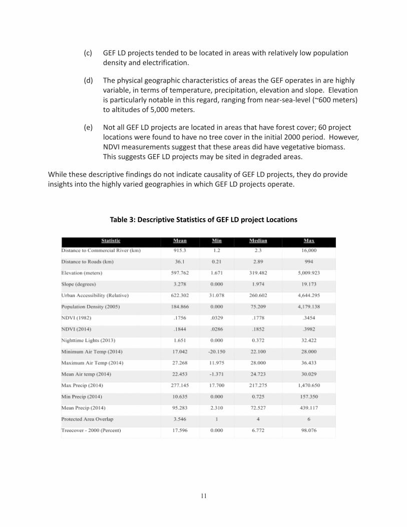
21. The results of a descriptive analysis examining the characteristics of GEF LD project locations (only considering projects for which an exact geographic location was available) can be found in table 3. These descriptors were based on the 25km areas around each GEF Land Degradation project. A few key findings are highlighted:

(a) GEF LD projects were located in areas that - on average - experienced positive increases in NDVI from 1982 to 2014. In this causal tree analysis we control for this upward trend by including information on the pre-project implementation trend in NDVI as well as the level of NDVI in the year prior to project implementation.

(b) All GEF LD projects were within 25km of a designated protected area of any kind, though only a subset were within 25km of protected areas with legally empowered designations.

11

(c) GEF LD projects tended to be located in areas with relatively low population density and electrification.

(d) The physical geographic characteristics of areas the GEF operates in are highly variable, in terms of temperature, precipitation, elevation and slope. Elevation is particularly notable in this regard, ranging from near-sea-level (~600 meters) to altitudes of 5,000 meters.

(e) Not all GEF LD projects are located in areas that have forest cover; 60 project locations were found to have no tree cover in the initial 2000 period. However, NDVI measurements suggest that these areas did have vegetative biomass. This suggests GEF LD projects may be sited in degraded areas.

While these descriptive findings do not indicate causality of GEF LD projects, they do provide insights into the highly varied geographies in which GEF LD projects operate.

Table 3: Descriptive Statistics of GEF LD project Locations

12

Causal Impacts

22. For each of the three models specified in table 2,C1, a Causal Tree is fit to identify the subsets of GEF LD projects for which differential treatment effects can be observed. This results in six different trees, which are summarized in this report. For the causal tree cases, we highlight the overall findings (i.e., if GEF LD projects in aggregate had positive, negative, or neutral impacts), as well as key findings of drivers of heterogeneity in causal impacts. For the case of random forests (C2) we contrast the results to facilitate a robustness check. Of key note is that, while each tree is unique, they all share the control variables identified in table 1 and summarized in table 3. If a variable is not present in a given tree, it can be interpreted as indicating that a particular variable was not key in defining subsets of the population for which the treatment varied in efficacy; however, the variable may still be important in mediating the impact in a single way across the entire population. Additionally, variables that are located in earlier splits in the tree tend to be more robust in terms of their importance in driving heterogeneity.

23. Not all observations were included in the Causal Tree analyses. The primary reason for observation removal was due to implementation date: in order to establish reasonable outcome measurements, the analysis was limited to projects that started in 2012 or earlier. Recognizing that even with this limitation significant variation can be expected based on the number of years a project has had to make an impact, we further control for the amount of time that elapsed between the measurement of outcome and the year of implementation.

Table 4: Propensity Model Results

13

24. A single propensity model was fit which describes the likelihood of treatment as measured by the covariate information, and is presented in table 4. This model was fit using a logistic regression, in which the response variable was a binary (GEF LD project presence or absence). While all variables are important in their role as controls in later stages of this analysis (see equation 3), of note is the significant relationship between the average minimum and maximum temperature with an increased likelihood of site selection, and a relationship between average temperature and a decreased probability of selection. Further, spatial patterns seem to play a role in site selection as evidenced by a significant relationship with longitude. Table 5 presents the pre- and post-matching difference between treatment and control groups along each ancillary variable, following a nearest neighbor matching strategy using the calculated propensity scores.

Table 5: Difference in GEF LD project LD locations and eligible locations at which no

25. Following the indicators suggested in the monitoring framework of the UNCCD for measuring land degradation (UNCCD 2015), three different metrics are used to ascertain the impact of GEF Land Degradation projects - Vegetation Density, Forest Cover, and Forest Fragmentation. Across the entire globe, GEF LD projects (a) increased NDVI by approximately 0.03 (relative to an average NDVI of 0.55), (b) reduced forest loss by 1.3% (relative to a global mean of 2.4% forest loss in all areas), and (c) increased the average size of forest patches by 0.25 kilometers (relative to a global mean of 7.3 square kilometers). We find that while the impact of GEF LD projects has been positive, there is considerable heterogeneity in impacts across different geographic contexts. Key finding for Vegetation Density included indications that projects in closer proximity to urban areas tended to be less effective; a minimum time lag

14

of 5.5 years was an important threshold for determining impact in some contexts (with some geographic locations requiring 7.5 years), and a tendency for areas with poorer initial conditions to improve to a greater degree. When Forest Cover was examined, it was found that a 4.5 year lag time was influential in determining effectivity. In the case of Fragmentation, it was found that the initial state of fragmentation - i.e., the pre-trend average - was a major factor in determining the heterogeneity in GEF LD project impacts.

26. The results of the causal tree analysis for NDVI can be seen in figure 6, and an online interactive view of these results can be found at http://labs.aiddata.org/GEF/treeBrowser/. In these results, we find that in aggregate GEF LD projects had a small, but positive impact on NDVI - specifically increasing NDVI by approximately 0.03 (relative to an average NDVI of 0.55). In addition to this aggregate finding, there are a number of findings in regard to the factors that mediated GEF LD impacts:

(a) In general, projects located in closer proximity to urban areas tended to be less effective than those located farther away.

(b) The period of time after project implementation was meaningful, with evidence suggesting that a minimum 5.5-year time lag is an important threshold for determining the degree of impact in some contexts; the maximum time lag found to be important was 7.5 years.

(c) While there is limited evidence of robustness, the analysis in this tree suggests that in limited contexts multifocal projects lead to improved outcomes.

(d) In some contexts, areas with poorer initial conditions (i.e., lower NDVI) saw greater improvement due to GEF LD projects.

(e) Environmental (slope, elevation, temperature, precipitation) and social characteristics (pop density, urban distance) all proved important in mediating the impact of GEF LD projects.

15

Figure 6: A Causal Tree representing impacts of GEF LD Projects on Vegetation Density (for easier viewing, an online application is available at

http://labs.aiddata.org/GEF/treeBrowser/).

27. Figure 7 shows the Causal Tree describing the impact of GEF LD projects on forest cover, and an interactive tree can be browsed at http://labs.aiddata.org/GEF/treeBrowser/. Each terminal node value represents the percent of tree cover loss that is attributable to GEF LD projects - i.e., a negative value indicates a GEF LD project slowed the rate of loss, while a positive value indicates it accelerated the rate of loss. As in the case of NDVI, globally there is a small but normatively positive impact attributable to GEF LD projects, which reduced forest loss by 1.3% (relative to a global mean of 2.4% forest loss in all areas). Key findings included:

(a) Evidence that projects with greater than 4.5 years of time since implementation had a stronger slowing effect on deforestation than more recent projects.

(b) Population density is a key factor driving heterogeneity in GEF LD project impacts, but relatively few GEF LD projects fell into locations with extremely low population densities (less than one individual per square km).

(c) There is some, limited evidence that GEF LD projects closer to urban areas were slightly more successful in mitigating forest cover losses in some geographic areas.

16

Figure 7: A Causal Tree representing impacts of GEF LD Projects on forest land cover (for easier viewing, an online application is available at http://labs.aiddata.org/GEF/treeBrowser/).

28. Figure 8 shows the Causal Tree describing the impact of GEF LD projects on forest fragmentation - specifically, the average forest patch size in 2014. This tree can also be viewed online at http://labs.aiddata.org/GEF/treeBrowser/. In this case, positive values indicate an increase in patch size as a product of a GEF LD project. Globally, this analysis suggests that GEF LD projects positively contributed to the patch size of forests on average, but with more significant heterogeneity in impacts when compared to the other two indicators examined - i.e., many projects had negative or neutral impacts. On average, GEF LD projects increased the average size of forest patches by 0.25 kilometers (relative to a global mean of 7.3 square kilometers). Unmeasured geographic factors - or, strong spillover effects - tended to have a large impact in the case of forest fragmentation, with the geographic latitude and longitude of a project being a consistent driver of relative efficacy of projects. GEF LD projects were also heavily influenced by the initial state of forest fragmentation - i.e., the pre-trend of average forest size is a major factor in determining the heterogeneity in GEF LD project impacts.

17

Figure 8: A Causal Tree representing impacts of GEF LD Projects on forest fragmentation (for easier viewing, an online application is available at

http://labs.aiddata.org/GEF/treeBrowser/).

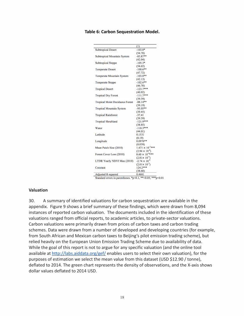
29. The model used to estimate carbon sequestration is detailed in section 6.4 (eq. 1), and the results of this model are shown in table 6. Approximately 47% of the variation in carbon sequestration across projects can be explained by the model at the project-location scale, the most conservative unit of measurement available for this analysis. While the model itself is purely predictive (and thus coefficient estimates and significance are not interpretable causally), the relative valuations of the different ecofloristic zones are of interest. These values indicate that the baseline values we use for estimation are highly variable by biome, an important factor for GEF LD projects that operate in semi-arid and humid tropical areas. Further, we find evidence supporting earlier academic literature that both forest cover loss and fragmentation are correlated with sequestration; NDVI plays a role in our prediction but we do not find significance in the relationship.

18

Table 6: Carbon Sequestration Model.

Valuation

30. A summary of identified valuations for carbon sequestration are available in the appendix. Figure 9 shows a brief summary of these findings, which were drawn from 8,094 instances of reported carbon valuation. The documents included in the identification of these valuations ranged from official reports, to academic articles, to private-sector valuations. Carbon valuations were primarily drawn from prices of carbon taxes and carbon trading schemes. Data were drawn from a number of developed and developing countries (for example, from South African and Mexican carbon taxes to Beijing’s pilot emission trading scheme), but relied heavily on the European Union Emission Trading Scheme due to availability of data. While the goal of this report is not to argue for any specific valuation (and the online tool available at http://labs.aiddata.org/gef/ enables users to select their own valuation), for the purposes of estimation we select the mean value from this dataset (USD $12.90 / tonne), deflated to 2014. The green chart represents the density of observations, and the X-axis shows dollar values deflated to 2014 USD.

19

Figure 9: Distribution of Carbon Valuations (per tonne sequestered) identified in the literature.

GEF LD project Valuations

31. Following the methodology outlined above, an estimate is performed for both overall project valuations as well as the valuation (and impact) for any given project location. Valuation for individual project locations can be viewed at http://labs.aiddata.org/gef/, as well as in figure 10. Based on the median estimate of $12.90 USD (2014) dollars per sequestered ton and a 25km area of influence, GEF LD Project locations were valued - on average - at USD $1,403,520, deflated to 2014 values. This ranged from a minimum of -$60,424, to a maximum of $4,108,650. At the project level, the mean valuation was $7,500,358, with a minimum of -$52,721 and a maximum of $48,653,058.

Figure 10: Estimated valuations of each GEF LD project location. Projects can be viewed in more detail, and monetary valuation assumptions can be modified, at

http://labs.aiddata.org/gef.

32. Over time, the value of a dollar of LD investment fluctuated across each of the three indicators assessed. In Figure 11, the average valuation of projects which started in a given year is presented (where valuation is defined based on impacts in 2014). In the case of fragmentation, projects which have been implemented most recently (2012) have apparent

20

higher returns when contrasted to earlier projects; the causation of this pattern is beyond the scope of this analysis but may provide helpful insights for practitioners seeking to identify successful strategies.

Figure 11: Shift in forest cover patch size attributable to USD $1 (2014) of GEF LD investment over time. Year represents the year of project implementation; valuation is determined based

on the impact of the project to 2014.

33. Figures 12 and 13 show the fluctuation in both NDVI and the rate of forest cover loss attributable to GEF LD projects, respectively. Projects which started in 2002, 2009, and 2012 all had notable negative impacts on NDVI, while projects in 2004 to 2007 and 2010-2011 tended to have positive impacts. In general, GEF LD projects have slowed deforestation, and projects which started in both 2002 and 2011 had an overall more positive effect (larger slowing of deforestation) per dollar of investment than other years. Across years, 2009 was generally the worst in terms of dollar efficacy, while projects which began in 2005 tended to have larger per-dollar efficiencies in terms of these three indicators. Because the models presented in this report control for other potential drivers of project variation (i.e., weather), this graph suggests significant variation in the efficiency of GEF LD projects over time. While it is outside the scope of this report to hypothesize what could cause these shifts, we note that an exploration of the projects which contributed to positive or negative fluctuations could be further examined to better understand these findings.

21

Figure 12: Shift in NDVI attributable to USD $1 (2014) of GEF LD investment over time. Year represents the year of project implementation; valuation is determined based on the impact

of the project to 2014.

Figure 13: Shift in forest cover loss attributable to USD $1 (2014) of GEF LD investment over

time. Year represents the year of project implementation; valuation is determined based on the impact of the project to 2014. Larger negative values indicate a slowing.

34. At the continental scale, there is also notable spatial variation in the impact of GEF LD projects. Table 7 describes this variation, which is generally reflective of the causal findings. Eastern Europe was the only region with universally negative findings; it also had one of the fewest number of high-precision GEF LD projects (3), limiting the interpretation of this finding. The majority of project locations were located in Africa and Asia; these had generally positive impacts on average excepting in the case of fragmentation. LAC, North and South America, and Oceania all had positive trends along all three indicators.

35. Table 7. Regional variation in GEF LD project impacts on indicators examined in this analysis. LAC indicates Latin America and the Caribbean. Red highlights indicate a negative result for GEF LD projects (i.e., increased deforestation); green highlights indicate a positive results for GEF LD projects (i.e., decreased deforestation). Significance is not calculated on a

22

per-region basis due to a highly variable N across regions. Because geographic location was the primary driver of fragmentation estimates, some proximate regions with low Ns have identical impact estimates.

Table 7: Regional Variation in GEF LD Project Impacts on Indicators.

Average change

attributable to GEF LD project

Locations

Geographic Region (Total N)

Rate of Forest Loss

Vegetative Productivity (NDVI)

Fragmentation (Mean Patch Size in Sq.Km.)

Africa (563) -.009274 0.01756905 -2.312

Asia (331) -.022815 0.02733678 -.1178

Eastern Europe (3) .002316 -0.01528436 -.0577

Europe (3) -.008403 -0.04980041 -.0577

LAC (3) -.028891 0.28456991 98.66

North America (90) -.024235 0.00435723 98.66

Oceania (56) -.010149 0.28456991 .2226

South America (57) -.001783 0.02748642 46.71

DISCUSSION

36. While this report provides evidence that, on average, GEF LD projects have mitigated or reversed negative LD processes, we also note the significant heterogeneity in these findings. We emphasize this heterogeneity to highlight the many opportunities for improvement which still exist by learning why and where GEF LD projects are leading to outcomes with relatively high benefits. These heterogeneities were found over both time - with project impacts being variable on a year-by-year basis - as well as space. As more observations are made available, we anticipate further drivers of heterogeneity in project impact could be observed (i.e., geopolitical issues; macro-economic trends).

37. The use of propensity score matching techniques to examine the causal effects of an intervention (i.e., international aid; a new business process; a new website design) has it's roots in econometric research from the early 1980s (Rosenbaum 1983). Since their introduction, propensity matching methods have been used for everything from better understanding customer retention and loyalty (Xerox, 2004), to the testing of new medical drugs (see Radiol

23

2015), to understanding supply chain dynamics (Falkowski 2009), and have been used extensively by researchers and practitioners seeking to understand the impact of aid (i.e. Gundersen and Sara 2016; Mensah et al. 2010). Most recently, these methods have become popular for testing websites such as Ebay, Facebook, and many more to establish and test optimal website designs (Taddy 2014; Backshy 2014; Briggs 2007). Practitioners have constantly refined matching approaches to understand causality, and the most recent wave of innovation has centered around heterogeneous impact effects - i.e., how an impact might vary across different geographic areas or groups of individuals (Athey and Imbens 2015). This is coupled with a push from geographic information scientists and practitioners to apply these approaches to geographic data to more cost-effectively ascertain environmental impacts, as well as considerable increases in the quality of satellite imagery available (i.e., Hansen et al. 2014). For example, using satellite and other geo-referenced data, propensity score matching and difference-in-difference approaches have been used to evaluate the impact of World Bank projects on forest change in key biodiversity areas (Buchanan et al. 2016), indigenous communities’ land rights on deforestation in Brazil (BenYishay et al. 2016), and land titling and land management programs in Ecuador (Buntaine et al. 2015).

38. Here, we advance the state of the art by applying a joint econometric and machine learning technique (specifically, Causal Trees) to examine how the impacts of GEF LD projects vary across geography and other factors. By examining the heterogeneity in impacts - rather than exclusively estimating overall effects - we show that (a) it is feasible to conduct global-scope, top-down analyses, as traditional methods for IE require pre-specification of possible factors driving heterogeneity, and (b) it is possible to distinguish between sources of positive and negative impacts.

39. We additionally employ state-of-the-art satellite imagery to detect changes as fine as 30 meters - a key factor when fragmentation and precise measurement of tree cover is of interest. By using GIS to couple this satellite imagery with a wide variety of other, globally available datasets (see table 1), we are able to provide geographic, contextual information that enables the identification of counterfactual cases. Further, by leveraging features of geographic variance itself - i.e., the trend that locations that are closer together tend to be more similar along unmeasured variables - we argue that this approach can mitigate - though not completely remove - many challenges associated with omitted variable biases.

40. By coupling three approaches - econometric propensity matching techniques, computer science machine learning algorithms, and GIS satellite imagery analysis and data integration, we further enable more accurate valuation of the impact of GEF LD projects across broader scopes than has been possible to date. By providing a methodology through which the impact of individual project locations can be estimated along multiple, value-relevant indicators, valuation efforts can focus on the single (but still very difficult) challenge of valuing shifts in indicator values, rather than methods to identify the precise percentage of a shift that is attributable to any given project.

24

41. This study has a number of remaining uncertainties and limitations which could be resolved through future work. First and foremost, this analysis is top-down, using only project information which is available at a global scale. While matching based on geography and geographic patterns can strongly mitigated omitted variable biases (i.e., by selecting treatment and control sites close together, and thus likely to experience similar conditions), nuanced, project-scale factors could still confound the results present here. We argue that, despite this limitation, the analysis presented here can be powerful in (a) identifying possible “bright spots” and “warning signs” at a relatively low cost; (b) identifying the geographic contexts in which GEF LD projects are most successful; and (c) providing strategic guidance as to the global and regional effectiveness of GEF LD projects. We strongly caution against using the information - or approach - detailed in this report to drive project-location level decision making without coupled, “bottom-up” analyses.

42. The scope across which GEF LD projects have impact is - frequently - unknown. Because limited geographic information has traditionally been collected on the exact geographic boundaries across which an intervention is performed, the underlying data used in this and similar analyses is point-based (i.e., a latitude and longitude coordinate). Because LD projects occur in a diffuse manner, an assumption as to the geographic extent a LD project might have an impact across is necessary lacking exact, geometric representations of the area across which project impact is anticipated. While we use a 25km buffer around each intervention, the collection of more precise geographic boundary information at the time of project implementation could result in more accurate impact estimates.

43. The Value Transfer Approach (Costanza et al. 2014) leveraged to estimate the total valuations of carbon sequestration is known as a “second best” option. More advanced approaches to estimating final valuations - including more explicit, regional modeling of value; stakeholder interviews; or economic-impact analyses - could provide better insights into the final estimated valuations of each project location. Further, the valuations estimated in this report only consider impacts on carbon sequestration, and do not take into consideration other benefits project locations may accrue - for example, co-benefits related to infrastructure development. Future analyses could leverage alternative remotely sensed datasets - such as Nighttime Lights - to construct indicators adequate to detect such co-benefits, or to further investigate questions of avoided emissions.

CONCLUSION

44. The findings of this report suggest that - in aggregate - GEF LD projects have had a positive impact on indicators of Land Degradation proposed by the UNCCD - specifically vegetative productivity (measured by NDVI) and forest cover (measured directly and by mean patch size). While these impacts vary substantially over space and time, we provide evidence that the GEF has contributed to increasing the total amount of carbon sequestered by forest cover and related biophysical processes. We estimate that - at a valuation of $12.90/tonne - GEF LD projects contributed $7.5 million USD (2014) on average to sequestration alone - well

25

above the average cost of most GEF LD projects ($4,182,887). We note that considerable heterogeneity exists in these findings.

45. Although examining the causal impact of international aid on environmental outcomes has been a central goal of many communities, there has been a limited engagement using spatially-explicit, geocoded aid information due to limitations in both data and methods (Corrado and Fingleton 2012; Athey and Imbens 2015a). These methodological limitations primarily stem from distinctions between modeling efforts seeking to predict relationships commonly taught and accepted by the geographic community (i.e., spatial regression or classification trees), and efforts which seek to establish causal relationships similarly taught and accepted by the economics community (i.e., propensity score matching or difference- in -difference modeling). Recent efforts have been undertaken to merge these disciplinary approaches (Drukker, Peter, and Prucha 2013; Buntaine, Hamilton, and Marco 2015b; D. Runfola et al. 2016), of which this report provides another example.

46. The methodology detailed in this report goes beyond these examples by providing an approach to capturing heterogeneity in impact effects - i.e., how GEF LD projects may vary in impact across different countries, regions, climate regimes, or human factors. This approach to learning based on historic GEF LD project implementations can additionally be flexibly applied to predict the potential impact of future projects (alongside concomitant uncertainties). As the cost of this style of analysis is lower than traditional impact evaluation, and enables the use of historic information, we believe it represents a screening step practitioners could take before project implementation.

APPENDIX I: DEFINITIONS

Defining Vegetation Productivity

1. There are many different approaches to approximating vegetation on a global scale, and satellites have been taking imagery that can be used for this purpose for over three decades. Of these approaches, the most frequently used - and applied in this study - is the Normalized Difference Vegetation Index (NDVI). The NDVI is a metric that has been used since the early 1970s, and is one of the simplest and most frequently used approaches to approximating vegetative biomass; further, it is recommended as an indicator by the GEF STAP (STAP 2014). NDVI measures the relative absorption and reflectance of red and near-infrared light from plants to quantify vegetation on a scale of -1 to 1, with vegetated areas falling between ~0.2 and 1. The reflectance by chlorophyll is correlated with plant health, and multiple studies have illustrated that it is generally also correlated with plant biomass. In other words, healthy vegetation and high plant biomass tend to result in high NDVI values (Dunbar 2009). Using NDVI as an outcome measure has a number of other benefits, including the long and consistent time periods for which it has been calculated. While the NDVI does have a number of challenges - including a propensity to saturate over densely vegetated regions, the potential for atmospheric noise (including clouds) to incorrectly offset values, and reflectances from bright soils providing misleading estimates - the popularity of this measurement has led to a number of improvements over time to offset many of these errors. This is especially true of

26

measurements from longer-term satellite records, such as those produced from MODIS and AVHRR (NASA 2015).

Defining Land Cover Change

2. Understanding the relationships between “process and pattern” - i.e., the links between drivers and observations of land cover change - has long been a focus of practitioners (Lambin et al., 2001; Liverman, 1998; Meyer and Turner, 1996; Nagendra et al., 2004; Turner et al., 2003). Land cover change has major implications for a broad range of phenomena, including the sustainability of human development, biogeochemical cycling, and levels of greenhouse gasses (Turner et al., 1995; UN-REDD, 2010). Investigating the many factors which influence land cover / use provides an avenue through which the human-environment interface can be better understood, but recent research has emphasized the lack of understanding of how anthropogenic processes influence land change (Nagendra et al., 2004). The impacts of land use / cover change on the vulnerability and sustainability of human-dominated landscapes is just beginning to be analyzed, and improving this understanding is a major goal of parties interested in understanding the consequences of land use change (Foley et al., 2005; GLP, 2010).

3. Both the geographic and development economics communities have sought to understand linkages between international development and land cover change, but often using different approaches and vocabulary. Within the geographic community, limited attention has been given to causal methodologies (including matching and difference-in-difference models), but rather focused on the (a) ability to accurately measure land cover change using satellite imagery (i.e., Borak, Lambin, and Strahler 2000; Strahler, Moody, and Lambin, n.d.; Christman et al. 2015; Rogan et al. 2003; Schwert et al. 2013), (b) impacts of spatial autocorrelation on model estimates (Miller, Arun, and Timmons Roberts 2012; Waldron et al. 2013), and (c) methods for predicting the impact(s) (and related uncertainties) of international aid on land change (Laurance et al. 2002; D. M. Runfola and Pontius 2013; van Asselen and Verburg 2013). Conversely, the development economics community has focused on the application of matching (Nelson and Chomitz 2011) and difference-in-difference (Pfaff 1999; Alix-Garcia, Shapiro, and Sims 2012; Nolte et al. 2013) techniques to establish evidence of causal relationships between international aid and land cover change - methods that follow similar approaches to clinical trials with treatment and control groups.

4. To capture land cover change in this analysis, we leverage an analysis performed by Hansen et al. (2013), in which LandSat imagery was fused with a number of other sources to capture 30-meter resolution, yearly estimates of tree cover loss. This land cover change analysis is widely leveraged to capture trends in deforestation, and represents one of the highest-resolution efforts for such measurements ever conducted. Further, as a global analysis, this product enables a precise calculation of both (a) tree cover in the year 2000, and (b) loss from 2000-2013 for every GEF LD project location.

27

Defining Forest Fragmentation

5. Classical forest fragmentation occurs when forest patches become smaller and more isolated than those in an undisturbed landscape, a process which can be driven by both natural and anthropogenic causes (Wulder et al. 2009). Academic and policy literature has repeatedly shown that fragmentation can have significant environmental implications (Mingshi et al. 2010; Garcia et al. 2005; Riitters et al. 2012). These implications include negative impacts on the biodiversity of an area (Hanski 2005, Zuidema, Sayer, & Dijkman 1996; Kolb & Diekmann 2005), negative effects on carbon sequestration (Diaz, Hector & Wardle 2009; Matthews, O’Connor, & Plantinga 2002), as well as modified risks of natural disasters such as fire (CITE). While there are many ways to describe fragmentation, in this analysis we examine the average patch size within the area of influence of GEF LD projects..

Defining Carbon Stocks and Sequestration

6. Forests contribute significantly to carbon sequestration through holding large carbon stocks. The combination of field-based estimates and remote sensing techniques has become the primary method of examining carbon stocks and carbon sequestration (Asner et al. 2010; Maselli et al. 2006; Muukkonen and Heiskanen 2005) because of difficulties with solely field-based estimates (Gibbs et al. 2007; Houghton 2005; Saatchi et al. 2007). Carbon stocks cannot be observed directly from satellite imagery; however, they can be estimated through examining factors associated with carbon stocks, particularly vegetation biomass. NDVI is one of the most widely used vegetation indices to estimate carbon stocks.

7. To date, empirical studies employing remote sensing to estimate carbon storage have done so at a local or country level and have shown that NDVI can strongly predict carbon stocks. For example, Myeong, Nowak, and Duggin (2006) estimate carbon storage among urban trees in Syracuse, New York, and find that NDVI explains 67 percent of the variation in field-based model estimates of carbon storage. Widayati, Ekadinata, and Syam (2005) examine the relation between carbon stocks and NDVI in Indonesia, motivated by the need to evaluate the effectiveness of community-based forest management projects in reducing deforestation. They found that NDVI explains 52.8 percent of the variation in carbon density. Wylie et al. (2003) use remote sensing to predict CO2 carbon fluxes in a sagebrush-steppe ecosystem in northeastern Idaho, finding that NDVI explains 79 percent of the variation in carbon flux, and including evapotranspiration as a predictor variable increased explanatory power to 82 percent. Gang et al. (2013) use NDVI, in combination with temperature and precipitation data, to estimate carbon stocks in the Xilingol grasslands in northern China, predicting carbon stocks with a 92.5 percent accuracy. For other studies that use NDVI to model carbon stocks, see Gilmanov et al. (2004) for estimates in Kazakhstan; Hunt et al. (2002, 2004) for estimates in Wyoming; Tan et al. (2007) and Piao et al. (2005) for estimates across China; Kanniah, Muhamad, and Kang (2014) and Hamdan et al. (2013) for estimates in Malaysia; and Verhegghen et al. (2012) for estimates of the Congo Basin.

8. Some researchers have moved beyond the local level to estimate global carbon stocks. Saatchi et al. (2011) estimate forest carbon stocks across 2.5 billion hectares of forests, covering

28

Africa, Asia, and South America. They rely on 14 remotely sensed variables (including NDVI) to estimate carbon stocks and field samples from 493 field sites to develop the model. They examine the predictive power of the 14 variables across geographic regions, where they find NDVI metrics explain most of the variation in carbon stocks in low biomass density forests. Other studies estimate carbon stocks around the world or at regional levels relying on remotely sensed data beyond NDVI. For example, see Baccini et al. (2012) and Ruesch and Gibbs (2008) for global estimates; Saatchi et al. (2007) for estimates of the Brazilian Amazon; Baccini et al. (2008), Brown and Gaston (1996), and Gibbs and Brown (2007a) for tropical Africa; and Brown, Iverson, and Prasad (2001) and Gibbs and Brown (2007b) for Southeast Asia. Further, some researchers have found that the relationships between NDVI, forest cover and carbon sequestration can be further permuted by forest fragmentation (Diaz, Hector & Wardle 2009; Matthews, O’Connor, & Plantinga 2002).

29

APPENDIX II: METHODS

Data Integration

9. Many of the datasets used in this analysis are collected at different spatial scales, necessitating an additional step of integration so that all observations can be analyzed at the scale of GEF LD projects (in this case, examining a 10km x 10km region around each project). To conduct this integration, we use the piecewise approximation procedure detailed in Goodchild et al. (1993):

eq. 6

where t is an index for the zone one is aggregating to (the GEF LD project area of interest), s is

an index for the set of zones one is aggregating from (i.e., a satellite pixels measuring NDVI), S is

the maximum index for all zones s, represents the value of interest at source zone s , is

the area of overlap between the two zones, is the area of the zone one is aggregating from,

and is the estimated value for the target zone. In our application, this procedure weights each

pixel of each dataset according to its overlap with each GEF LD project.

Causal Model

10. Classification and Regression Tree approaches have been commonly employed over the last two decades to aid in the classification of remotely sensed imagery (Friedl and Brodley 1997; McIver and Friedl 2002; Gamba and Herold 2009). Here, we employ Causal Trees - a novel version of a CART which enables causal inferential analyses. Causal Trees are implemented in a multiple step process, detailed below but simply summarized as (a) deriving a metric which indicates similarity between treatment and control groups; (b) using this metric to match pairs of treatment and control units via a tree; (c) contrasting the outcome of treated units to control units within every terminal node of the tree. Figure 4 shows an example drawn from exploratory research in which a Causal Tree is applied to a limited subset of international aid, examining aid’s impact on a maximum observed NDVI value. This figure serves as an illustrative example of the outputs of Causal Tree based approaches to identifying how impact effects may differ across a dataset. Unlike traditional econometric approaches in which interaction terms must be pre-specified to estimate differential impact effects, here clusters of similar treatment and control units are identified dynamically. Further, by including geographic factors in these trees (i.e., latitude and longitude), many unobserved geographic characteristics can be captured. As in a traditional econometric analysis in which variables can be identified as statistically significant, here variables which are significant (defined as the variables which describe the most variance in the data; see eq. 4) are represented in the tree. All variables are controlled for through the propensity adjustment of the outcome (see eq. 3).

30

11. The primary distinction between Causal Trees and more traditional tree-based classifiers lies in the criterion along which splits in the tree are selected. Consider a data set with n independently and identically distributed units with , and for each unit a vector of relevant covariates are measured. In a simplified case where all things other than treatment are being constant, to estimate a causal effect for each geographic location i we can use the Rubin causal model (Rubin 1997) and consider the treatment effect as being equal to:

eq. 7

where is an indicator of if a unit of observation i received aid (1) or did not (0). Following

this simplified model, we define the expected heterogeneous causal effect for any set of units as

(Athey and Imbens 2015b):

eq. 8

Athey and Imbens show that one can estimate the causal effect as where

the transformed outcome is defined as:

eq. 9

and the propensity score function is defined as . Several

approaches to estimate the propensity score can be selected (Rosenbaum and Rubin 1983; Pan

and Bai 2015) - here, we estimate using logistic regression. Once the propensity score and

have been estimated, many authors (Su et al. 2009; Athey and Imbens 2015; Wagner and

Athey 2015; Denil et al. 2014; Meinhausen 2016; Biau 2012; Wagner et al. 2014) have illustrated

that classification and regression trees can be used to isolate treatment effects within sets of

similar units. These trees seek to classify units of observation into clusters that are similar along

covariate axes, following different splitting and optimization rules.

12. Using the propensity score, Causal Tree approaches derive a transformed outcome variable, , and use this to generate tree splits instead of (the traditionally used) . This transformed outcome is calculated following eq. 3. The CT replaces the traditional MSE optimization criterion in trees by seeking to minimize the sum of in each terminal node, where represents the estimated average treatment impact within a given node, i.e.:

eq. 10

31

13. This new error term is then used to split the tree in a way identical to traditional regression trees, and provides a tree which increases the similarity of control and treated units within each node, as well as node-specific estimates of impacts.

APPENDIX III: GEOCODING INTERNATIONAL AID

This project leveraged the AidData development finance and international aid geocoding

methodology. In 2010, AidData developed a methodology for georeferencing development

projects that IATI later revised and adopted as its global reporting standard. Leveraging a team

of trained geocoders, the geocoding methodology and online toolkit relies on a double-blind

coding system, where two experts employ a defined hierarchy of geographic terms and

independently assign uniform latitude and longitude coordinates, precision codes, and

standardized place names to each geographic feature. If the two code rounds disagree, the

project is moved into an arbitration round where a geocoding project manager reconciles the

codes to assign a master set of geocodes for all of the locations described in the available

project documentation. This approach also captures geographic information at several levels—

coordinate, city, and administrative divisions—for each location, thereby allowing the data to be

visualized and analyzed in different ways depending upon the geographic unit of interest. Once

geographic features are assigned coordinates, coders specify a location class ranging from 1 to 4

for categories including administrative regions or topographical features along with a location

type specifying the exact feature (e.g., airport, second order administrative zone, etc.). Coders

then determine the location’s geographic exactness value of either 1 (exact) or 2 (approximate).

14. AidData performs many procedures to ensure data quality, including de-duplication of projects and locations, correcting logical inconsistencies (e.g. making sure project start and end dates are in proper order), finding and correcting field and data type mismatches, correcting and aligning geocodes and project locations within country and administrative boundaries, validating place names and correcting gazetteer inconsistencies, deflating financial values to constant dollars across projects and years (where appropriate), strict version control of intermediate and draft data products, semantic versioning to delineate major and minor versions of various geocoded datasets, and final review by a multidisciplinary working group.

Appendix IV: Robustness Checks

15. In order to test the robustness of the results presented in this document, two different approaches were followed. First, a random forest (RF) implementation of the Causal Tree (CT) approach was implemented. Second, the analysis was repeated using the traditional Causal Tree approach, but using the watershed in which each unit fell as the unit of observation (i.e., watersheds with no GEF LD projects contained within them were matched to watersheds that contained GEF LD projects). The RF-CT approach takes a different approach to uncertainty than a traditional Causal Tree. In the Random Forest, a large number of trees (in this case, 10,000) are fit, each time fitting using a different subset of the data. This approach provides two

32

advantages. First, it allows for an estimate of the importance of different variables across trees - i.e., it can be established which variables seem to drive heterogeneity in the impacts of GEF LD projects. Second, it provides a range of possible values that could be estimated for each GEF LD project, given the potential for different matches across different subsets of the data. From these two point of evidence, it is possible to provide insight into the relative certainty of claims for any given observation, as well as the structure of the tree found in the traditional CT approach. The primary drawback of the RF-CT is that it does not provide a single tree for interpretation (as in the above CT approach), thus limiting potential insights regarding the exact contexts in which projects succeed and fail.

Figure 14: The result of a random forest for one GEF observation.

Each of 1000 iterations are plotted

16. Figure 14 illustrates an example of how uncertainty due to tree construction can be captured for each individual GEF LD project location. We can use this distribution to calculate the percent of observations within - for example - 1 standard deviation of the mean. While this cannot be interpreted as a statistical significance (due to the lack of parametric assumptions in the underlying models and distributions, as well as differential aims of the tests), if a high percent of observations fall in this area, we illustrate that our findings are generally robust with regard to the shape of the tree. This analysis is conducted for each of the three focal areas, as summarized in table 8.

33

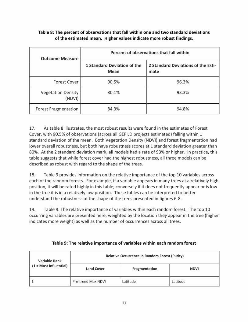
Table 8: The percent of observations that fall within one and two standard deviations of the estimated mean. Higher values indicate more robust findings.

Outcome Measure

Percent of observations that fall within

1 Standard Deviation of the Mean

2 Standard Deviations of the Esti-mate

Forest Cover 90.5% 96.3%

Vegetation Density (NDVI)

80.1% 93.3%

Forest Fragmentation 84.3% 94.8%

17. As table 8 illustrates, the most robust results were found in the estimates of Forest Cover, with 90.5% of observations (across all GEF LD projects estimated) falling within 1 standard deviation of the mean. Both Vegetation Density (NDVI) and forest fragmentation had lower overall robustness, but both have robustness scores at 1 standard deviation greater than 80%. At the 2 standard deviation mark, all models had a rate of 93% or higher. In practice, this table suggests that while forest cover had the highest robustness, all three models can be described as robust with regard to the shape of the trees.

18. Table 9 provides information on the relative importance of the top 10 variables across each of the random forests. For example, if a variable appears in many trees at a relatively high position, it will be rated highly in this table; conversely if it does not frequently appear or is low in the tree it is in a relatively low position. These tables can be interpreted to better understand the robustness of the shape of the trees presented in figures 6-8.

19. Table 9. The relative importance of variables within each random forest. The top 10 occurring variables are presented here, weighted by the location they appear in the tree (higher indicates more weight) as well as the number of occurrences across all trees.

Table 9: The relative importance of variables within each random forest

Variable Rank

(1 = Most Influential)

Relative Occurrence in Random Forest (Purity)

Land Cover Fragmentation NDVI

1 Pre-trend Max NDVI Latitude Latitude

34

2 Year Year 2000 Tree Cover

3 Pre-trend Avg Air Temp Post Implementation Time Pre-trend Max NDVI

4 Latitude Slope Pre-trend Min Temp

5 Post Implementation Time Pre-level Min Air Temp Pre-trend Max Temp

6 Slope Pre-level Avg Air Temp Elevation

7 Longitude 2000 Tree Cover Year

8 Urban Accessibility Pre-trend Avg Air Temp Urban Accessibility

9 Population Density (2000) Longitude Pre-trend Min Precip

10 Pre-trend Average NDVI Elevation Post Implementation Time

11+ All other variables All other variables All other variables

20. Table 9 illustrates the robustness of the shape of the trees - specifically, if claims regarding a particular split can be determined to be robust. Of note is that post-implementation time appears in all three models as being an important factor in distinguishing GEF LD project impacts. Additional variables that are important across multiple outcome measures included the year of implementation (suggesting a difference in the effectiveness of projects over time), geographic factors (latitude and longitude), and a variety of physical and environmental characteristics.

ACKNOWLEDGEMENTS

21. We would like to thank valuable team members Geeta Batra, Anupam Anand and the Director Juha Uitto (GEF), Dan Runfola, Jyoteshwar Nagol, Ariel BenYishay, Seth Goodman, and the AidData Data Team (Zhonghui Lv, Lauren Harrison, Alex Kappel, Sid Ghose, Brooke Russell). This work was performed in part using computational facilities at the College of William and Mary which were provided with the assistance of the National Science Foundation, the Virginia Port Authority, Virginia's Commonwealth Technology Research Fund and the Office of Naval Research.

VALUATION SOURCE DATA

The full list of valuations considered for carbon can be found at:

https://docs.google.com/spreadsheets/d/1-

kUFMuirvMLfsdMGd01i50oj1IMvfiU0PBg3YADfWxM/pubhtml

35

BIBLIOGRAPHY

Alix-Garcia, J. M., E. N. Shapiro, and K. R. E. Sims. 2012. “Forest Conservation and Slippage:

Evidence from Mexico’s National Payments for Ecosystem Services Program.” Land

Economics 88 (4): 613–38.

Andam, Kwaw S., Paul J. Ferraro, Alexander Pfaff, G. Arturo Sanchez-Azofeifa, and Juan A.

Robalino. 2008. “Measuring the Effectiveness of Protected Area Networks in Reducing

Deforestation.” Proceedings of the National Academy of Sciences of the United States of

America 105 (42): 16089–94.

Athey, Susan, and Guido Imbens. 2015a. “Recursive Partitioning for Heterogeneous Causal

Effects.” arXiv:1504.01132 [stat], April. http://arxiv.org/abs/1504.01132.

———. 2015b. “Recursive Partitioning for Heterogeneous Causal Effects.”

arXiv:1504.01132 [stat], April. http://arxiv.org/abs/1504.01132.

Borak, J. S., E. F. Lambin, and A. H. Strahler. 2000. “The Use of Temporal Metrics for Land

Cover Change Detection at Coarse Spatial Scales.” International Journal of Remote Sensing

21 (6-7): 1415–32.

Buntaine, Mark T. 2011. “Does the Asian Development Bank Respond to Past

Environmental Performance When Allocating Environmentally Risky Financing?” World

Development 39 (3): 336–50.

Buntaine, Mark T., Stuart E. Hamilton, and Millones Marco. 2015a. “Titling Community

Land to Prevent Deforestation: An Evaluation of a Best-Case Program in Morona-Santiago,

Ecuador.” Global Environmental Change: Human and Policy Dimensions 33: 32–43.

———. 2015b. “Titling Community Land to Prevent Deforestation: An Evaluation of a Best-

Case Program in Morona-Santiago, Ecuador.” Global Environmental Change: Human and

Policy Dimensions 33: 32–43.

Christman, Zachary, Christman Zachary, Rogan John, J. Ronald Eastman, and B. L. Turner II.

2015. “Quantifying Uncertainty and Confusion in Land Change Analyses: A Case Study

from Central Mexico Using MODIS Data.” GIScience and Remote Sensing, 1–28.

Corrado, L., and B. Fingleton. 2012. “Where Is the Economics in Spatial Econometrics?”

Journal of Regional Science. Wiley Online Library.

http://onlinelibrary.wiley.com/doi/10.1111/j.1467-9787.2011.00726.x/full.

36

Drukker, David M., Egger Peter, and Ingmar R. Prucha. 2013. “On Two-Step Estimation of a

Spatial Autoregressive Model with Autoregressive Disturbances and Endogenous

Regressors.” Econometric Reviews 32 (5-6): 686–733.

Friedl, M. A., and C. E. Brodley. 1997. “Decision Tree Classification of Land Cover from

Remotely Sensed Data.” Remote Sensing of Environment 61 (3): 399–409.

Gamba, Paolo, and Martin Herold. 2009. Global Mapping of Human Settlement:

Experiences, Datasets, and Prospects. CRC Press.

Kapur, Devesh, John Lewis, and Richard Webb. 2010. The World Bank: Its First Half

Century (Vol. I & II). Brookings Institution Press.

Kareiva, P., A. Chang, and M. Marvier. 2008. “Development and Conservation Goals in

World Bank Projects.” Science. academia.edu.

http://www.academia.edu/download/37393500/PovertyandConservation._2008.pdf.

Laurance, William F., Ana K. M. Albernaz, Schroth Gotz, Philip M. Fearnside, Bergen Scott,

Eduardo M. Venticinque, and Carlos Da Costa. 2002. “Predictors of Deforestation in the

Brazilian Amazon.” Journal of Biogeography 29 (5-6): 737–48.

McIver, D. K., and M. A. Friedl. 2002. “Using Prior Probabilities in Decision-Tree

Classification of Remotely Sensed Data.” Remote Sensing of Environment 81 (2-3): 253–61.

McShane, Thomas O., Paul D. Hirsch, Tran Chi Trung, Alexander N. Songorwa, Ann Kinzig,

Bruno Monteferri, David Mutekanga, et al. 2011/3. “Hard Choices: Making Trade-Offs

between Biodiversity Conservation and Human Well-Being.” Biological Conservation 144

(3): 966–72.

Mellor, John W. 2005. “Warwick J. McKibbin and Peter J. Wilcoxen. Climate Change Policy

after Kyoto . Washington, DC: Brookings Institution Press, 2002.Tamar L. Gutner. Banking

on the Environment: Multilateral Development Banks and Their Environmental

Performance in Central and Eastern Europe . Cambridge, MA: MIT Press, 2002. $24.95

(paper).” Economic Development and Cultural Change 53 (2): 540–43.

Miller, Daniel C., Agrawal Arun, and J. Timmons Roberts. 2012. “Biodiversity, Governance,

and the Allocation of International Aid for Conservation.” Conservation Letters 6 (1): 12–

20.

37

Nelson, Andrew, and Kenneth M. Chomitz. 2011. “Effectiveness of Strict vs. Multiple Use

Protected Areas in Reducing Tropical Forest Fires: A Global Analysis Using Matching

Methods.” PloS One 6 (8): e22722.

Nolte, Christoph, Arun Agrawal, Kirsten M. Silvius, and Britaldo S. Soares-Filho. 2013.

“Governance Regime and Location Influence Avoided Deforestation Success of Protected

Areas in the Brazilian Amazon.” Proceedings of the National Academy of Sciences of the

United States of America 110 (13): 4956–61.

Pan, W., and H. Bai. 2015. Propensity Score Analysis: Fundamentals and Developments.

Guilford Publications.

Pfaff, Alexander S. P. 1999. “What Drives Deforestation in the Brazilian Amazon?” Journal

of Environmental Economics and Management 37 (1): 26–43.

Rindfuss, Ronald R., Stephen J. Walsh, B. L. Turner 2nd, Jefferson Fox, and Vinod Mishra.

2004. “Developing a Science of Land Change: Challenges and Methodological Issues.”

Proceedings of the National Academy of Sciences of the United States of America 101 (39):

13976–81.

Rogan, John, Rogan John, Miller Jennifer, Stow Doug, Franklin Janet, Levien Lisa, and

Fischer Chris. 2003. “Land-Cover Change Monitoring with Classification Trees Using

Landsat TM and Ancillary Data.” Photogrammetric Engineering & Remote Sensing 69 (7):

793–804.

Rosenbaum, Paul R., and Donald B. Rubin. 1983. “The Central Role of the Propensity Score

in Observational Studies for Causal Effects.” Biometrika 70 (1): 41–55.

Rubin, Donald B. 1997. “Estimating Causal Effects from Large Data Sets Using Propensity

Scores.” Annals of Internal Medicine 127 (8_Part_2): 757–63.

Runfola, Dan, Jeff Tanner, Matthias Leu, Graeme Buchanan, and Ariel BenYishay. 2016.

“Valuing Environmental Impacts of World Bank Projects: A Case Study of Integrating Value

for Money Analysis into Impact Evaluations.” World Bank.

Runfola, D. M., and R. G. Pontius Jr. 2013. “Quantifying the Temporal Instability of Land

Change Transitions.” International Journal of GIS.

Schwert, B., J. Rogan, N. M. Giner, Y. Ogneva-Himmelberger, S. D. Blanchard, and C.

Woodcock. 2013. “A Comparison of Support Vector Machines and Manual Change

38

Detection for Land-Cover Map Updating in Massachusetts, USA.” Remote Sensing Letters

4 (9): 882–90.

Shandra, J. M. 2007. “The World Polity and Deforestation: A Quantitative, Cross-National

Analysis.” International Journal of Comparative Sociology 48 (1): 5–27.

Shandra, J. M., E. Shircliff, and B. London. 2011. “World Bank Lending and Deforestation: A

Cross-National Analysis.” International Sociology: Journal of the International Sociological

Association 26 (3): 292–314.

Shen, Changyu, Yang Hu, Xiaochun Li, Yadong Wang, Peng-Sheng Chen, and Alfred E.

Buxton. 2016. “Identification of Subpopulations with Distinct Treatment Benefit Rate

Using the Bayesian Tree.” Biometrical Journal. Biometrische Zeitschrift, June.

doi:10.1002/bimj.201500180.

Spence, Michael, Patricia Clarke Annez, and Robert M. Buckley. 2008. Urbanization and

Growth. World Bank Publications.

Staff, The Plos One. 2014. “Correction: Inferring Tree Causal Models of Cancer Progression

with Probability Raising.” PloS One 9 (12): e115570.

Strahler, A. H., A. Moody, and E. Lambin. n.d. “Land Cover and Land-Cover Change from

MODIS.” In 1995 International Geoscience and Remote Sensing Symposium, IGARSS ’95.

Quantitative Remote Sensing for Science and Applications.

doi:10.1109/igarss.1995.521802.

Turner, B. L., 2nd, Eric F. Lambin, and Anette Reenberg. 2007. “The Emergence of Land

Change Science for Global Environmental Change and Sustainability.” Proceedings of the

National Academy of Sciences of the United States of America 104 (52): 20666–71.

Turner, B., and W. B. Meyer. 1991. “Land Use and Land Cover in Global Environmental

Change.” International Social Science Journal. asu.pure.elsevier.com.

http://asu.pure.elsevier.com/en/publications/land-use-and-land-cover-in-global-

environmental-change-considerat.

UNCCD. 2015. “The Land Degradation Neutrality Project.”

http://www.unccd.int/en/Stakeholders/private_sector/Documents/Land%20Degradation

%20Neutrality.pdf.

39

van Asselen, Sanneke, and Peter H. Verburg. 2013. “Land Cover Change or Land-Use

Intensification: Simulating Land System Change with a Global-Scale Land Change Model.”

Global Change Biology 19 (12): 3648–67.

Wade, Robert Hunter. 2003. “Review: Promoting Environmental Sustainability in

Development: An Evaluation of the World Bank’s Performance.” Environment and Planning

A 35 (4): 759–60.

Waldron, Anthony, Arne O. Mooers, Daniel C. Miller, Nate Nibbelink, David Redding, Tyler

S. Kuhn, J. Timmons Roberts, and John L. Gittleman. 2013. “Targeting Global Conservation

Funding to Limit Immediate Biodiversity Declines.” Proceedings of the National Academy

of Sciences of the United States of America 110 (29): 12144–48.