Value-at-Risk and Expected Shortfall

Presentation at Finansforening’s Network for Performance Measurement

Copenhagen, June 8, 2015

Søren Plesner, CFA

sp@spfk.dk

1

The Moderator

• Soren Plesner

• M.Sc. (Economics)

• CFA, FRM & PRM

• External Lecturer at the Copenhagen Business School

• Founder of Upside (SPFK Financial Knowhow)

• Previously – BASISPOINT

– SimCorp

– Danske Bank

– IBM

• www.spfk.dk

• sp@spfk.dk

2

Some people Don’t Like CFA’s!

• So when you see a quantitative “expert”, shout for help, call for his disgrace, make him accountable. Do not let him hide behind the diffusion of responsibility. Ask for the drastic overhaul of business schools (and stop giving funding). Ask for the Nobel prize in economics to be withdrawn from the authors of these theories, as the Nobel’s credibility can be extremely harmful. Boycott professional associations that give certificates in financial analysis that promoted these methods – Nassim Nicholas Taleb and Pablo Triana i Financial Times den 7. december 2008

3

Not Much Confidence in VaR Either!

• Remove Value-at-Risk books from the shelves – quickly. Do not be afraid for your reputation. Please act now. Do not just walk by. Remember the scriptures: “Thou shalt not follow a multitude to do evil” – Nassim Nicholas Taleb and Pablo Triana i Financial Times den 7. december 2008

4

Outline

• What Is Value at Risk (VaR)?

• Problems with VaR

• Value at Risk in Financial Regulation

• The Move to Expected Shortfall

• Performance Measurement – In banks

– In asset portfolios

5

Value-at-Risk

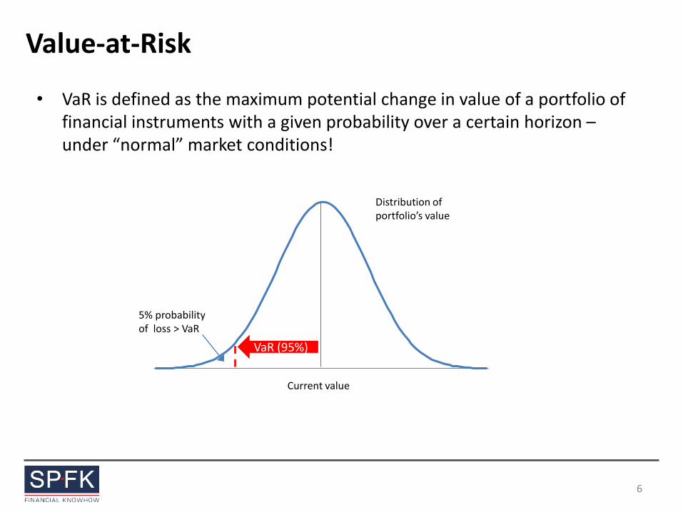
• VaR is defined as the maximum potential change in value of a portfolio of financial instruments with a given probability over a certain horizon – under “normal” market conditions!

Current value

VaR (95%)

5% probability of loss > VaR

Distribution of portfolio’s value

6

VaR – Important Applications

• Risk management – Risk assessment

– Limit setting

• Regulatory requirements – Trading book capital charges

• Evaluating the performance of risk takers – RAPM

– RAROC

– Reward to VaR ratio

– ………

7

Steps in Constructing VaR

• Mark-to-market of current position/portfolio

• Measure the variability of the risk factor(s)

• Set the time horizon

• Set the confidence level

• Calculate VaR for single position(s)

• Calculate total portfolio VaR using correlation matrix

• Report maximum potential loss (VaR)

• Perform stress testing of assumptions

8

Financial Markets – Empirical Facts

• Financial return distributions are leptokurtotic – have heavier tails and a higher peak than a normal distribution.

• Returns are typically negatively skewed

• Squared returns have significant autocorrelation – i.e. volatilities of market factors tend to cluster.

9

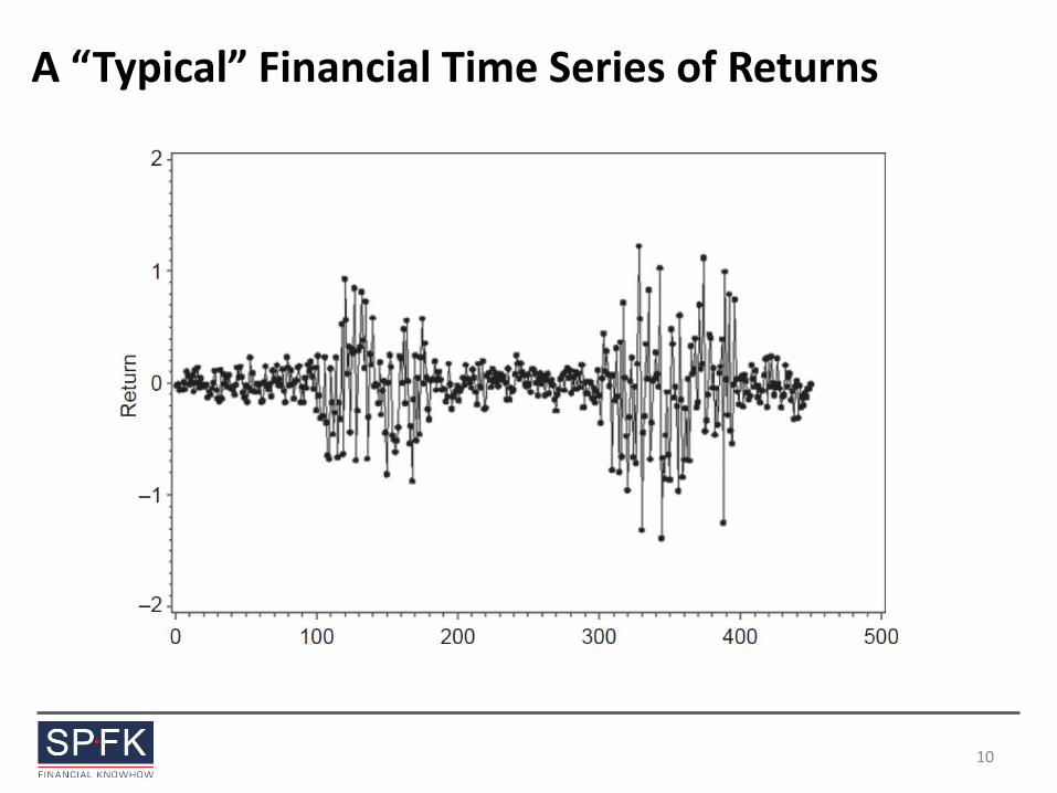
A “Typical” Financial Time Series of Returns

10

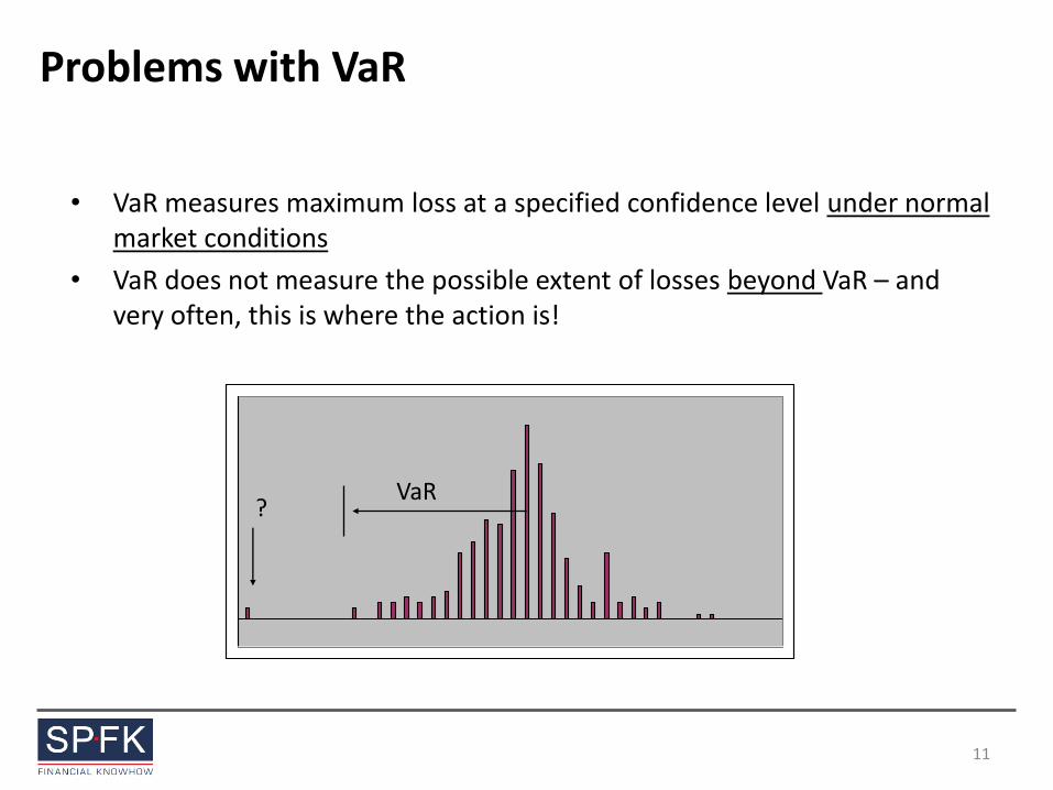
Problems with VaR

• VaR measures maximum loss at a specified confidence level under normal market conditions

• VaR does not measure the possible extent of losses beyond VaR – and very often, this is where the action is!

VaR ?

11

Surprised?

• ”We are seeing things that were 25-standard deviation moves, several days in a row” – David Viniar, CFO of Goldman Sachs, August 2007

12

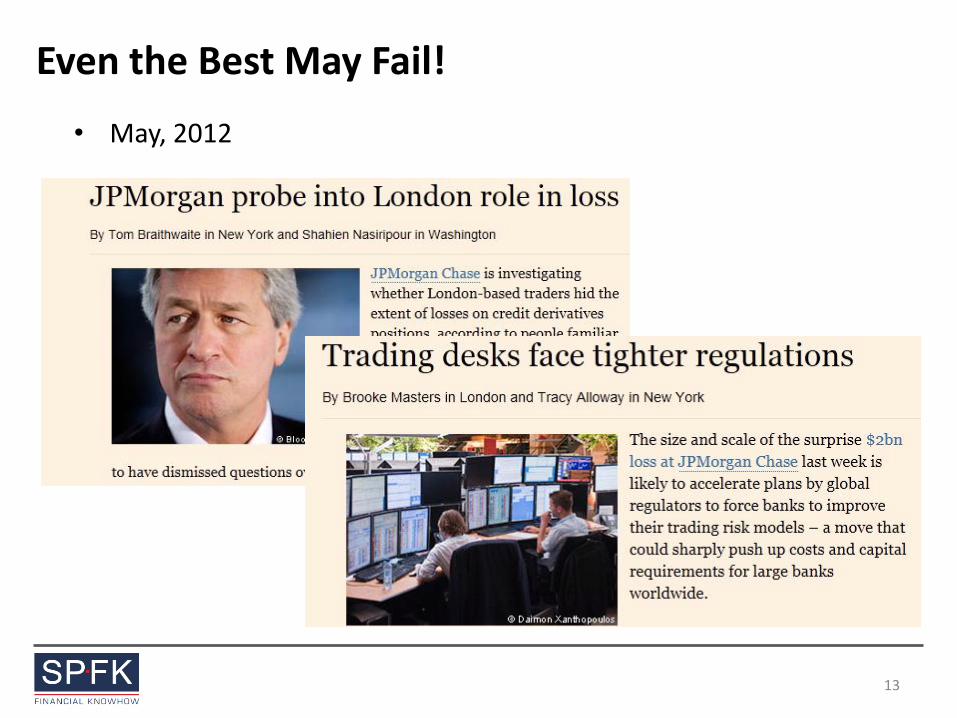
Even the Best May Fail!

• May, 2012

13

VaR Methodologies – Broad Categories

• Parametric (RiskMetrics and GARCH)

• Extreme Value Theory

• Nonparametric – Historical Simulation

– Monte Carlo simulation

14

VaR in Financial Banking Regulation (Basel)

• VaR was introduced I banking regulation in the “market risk amendment” in 1996

• Banks’ balance sheets were divided into “banking books” and a “trading books”

• 99% 10-day VaR capital charge for “market risk” – Subject to backtesting an stress testing

• But VaR (and stress testing failed completely to capture risks in the run-op to the financial crisis

• Regulatory reactions – Basel 2.5

– Trading Book Review

15

16

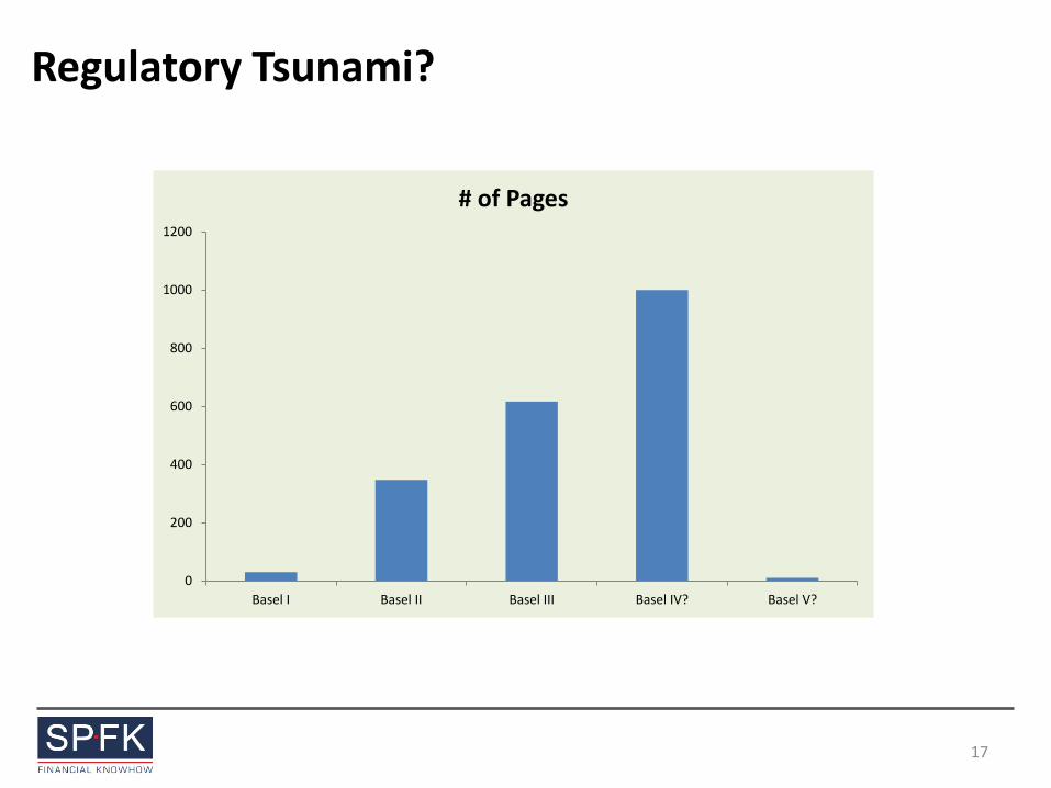
Regulatory Tsunami?

0

200

400

600

800

1000

1200

Basel I Basel II Basel III Basel IV? Basel V?

# of Pages

17

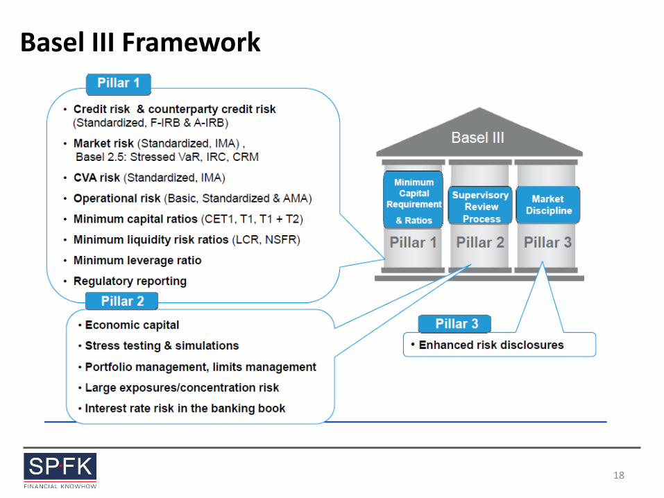
Basel III Framework

18

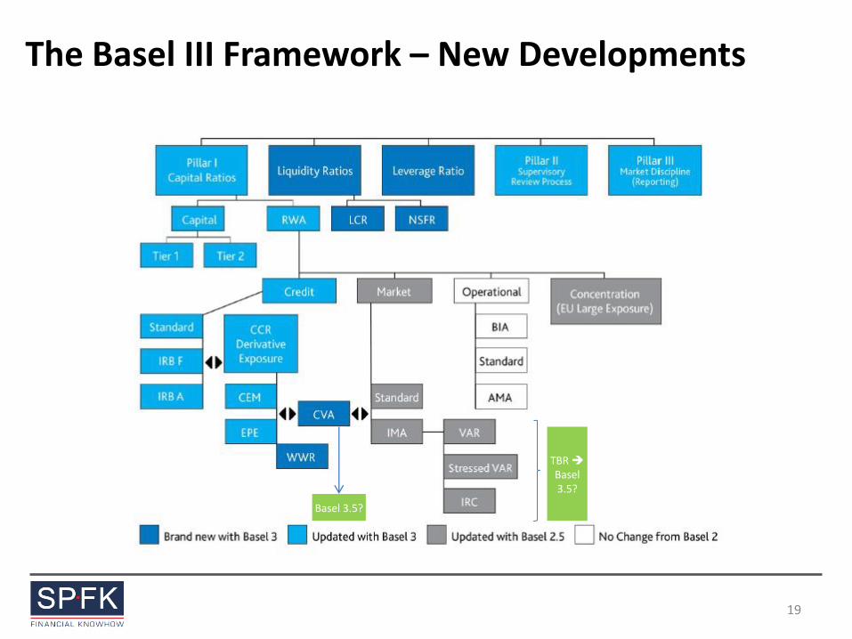
The Basel III Framework – New Developments

Basel 3.5?

TBR Basel 3.5?

19

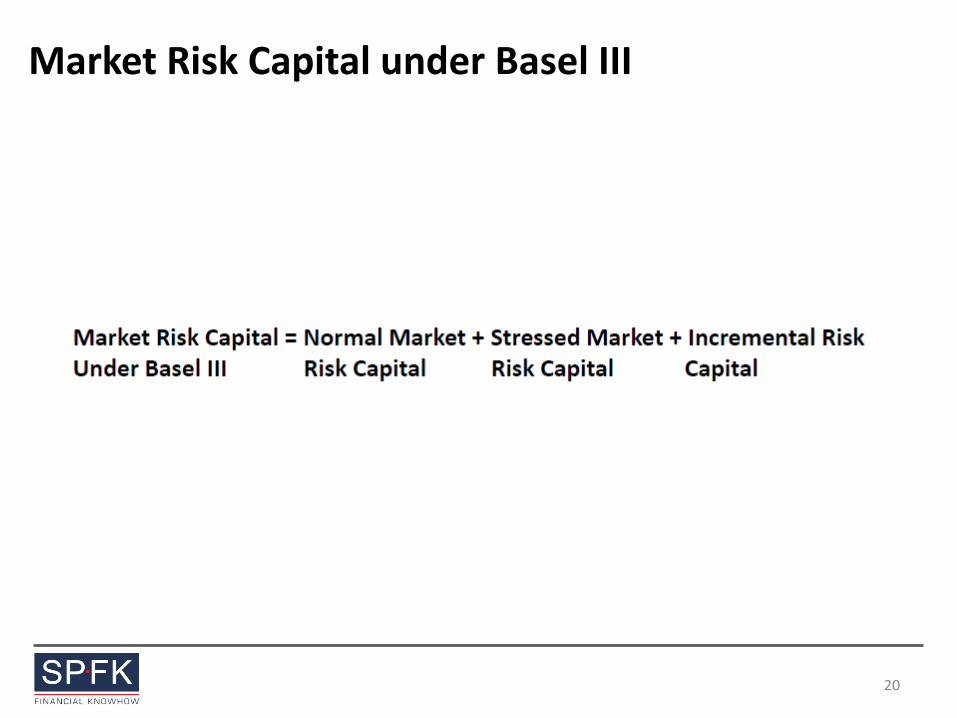
Market Risk Capital under Basel III

20

Stressed VaR

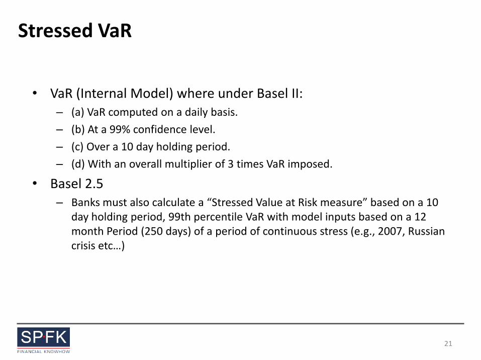
• VaR (Internal Model) where under Basel II: – (a) VaR computed on a daily basis.

– (b) At a 99% confidence level.

– (c) Over a 10 day holding period.

– (d) With an overall multiplier of 3 times VaR imposed.

• Basel 2.5 – Banks must also calculate a “Stressed Value at Risk measure” based on a 10

day holding period, 99th percentile VaR with model inputs based on a 12 month Period (250 days) of a period of continuous stress (e.g., 2007, Russian crisis etc…)

21

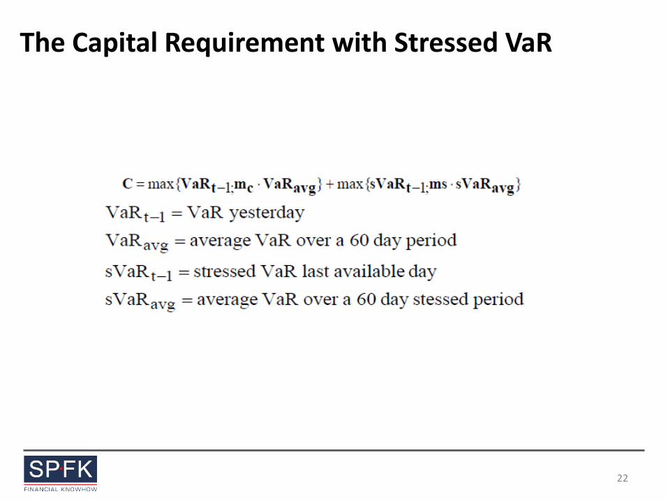
The Capital Requirement with Stressed VaR

22

Stressed VaR - Example

• Portfolio of 2 stocks – IBM , MV = 20M

– Ford, MV = 10m

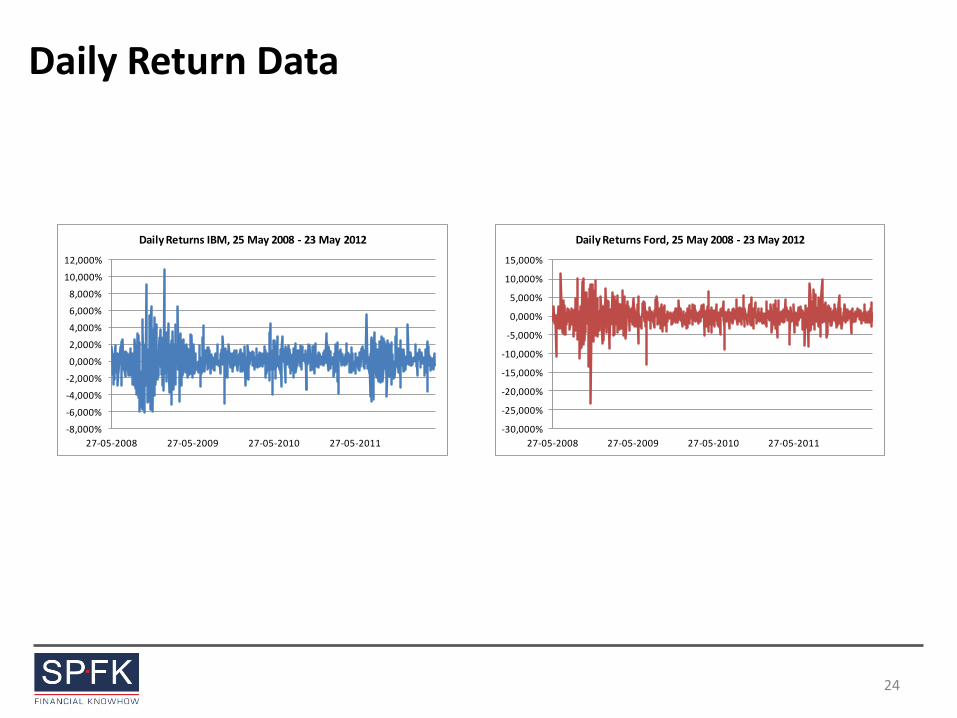
• VaR calculated used daily return data 23 May 2011 – 23 May 2012

• Stressed VaR calculated used daily return data 27 May 2008 – 27 May 2009 – ”the worst period in living memory”

23

Daily Return Data

-8,000%

-6,000%

-4,000%

-2,000%

0,000%

2,000%

4,000%

6,000%

8,000%

10,000%

12,000%

27-05-2008 27-05-2009 27-05-2010 27-05-2011

Daily Returns IBM, 25 May 2008 - 23 May 2012

-30,000%

-25,000%

-20,000%

-15,000%

-10,000%

-5,000%

0,000%

5,000%

10,000%

15,000%

27-05-2008 27-05-2009 27-05-2010 27-05-2011

Daily Returns Ford, 25 May 2008 - 23 May 2012

24

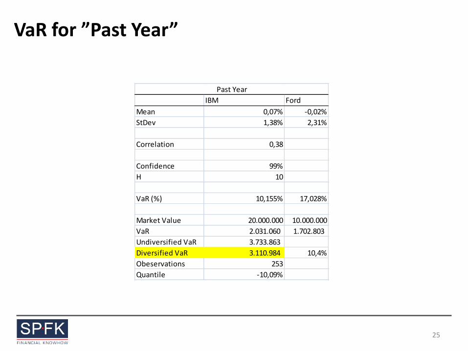
VaR for ”Past Year”

IBM Ford

Mean 0,07% -0,02%

StDev 1,38% 2,31%

Correlation 0,38

Confidence 99%

H 10

VaR (%) 10,155% 17,028%

Market Value 20.000.000 10.000.000

VaR 2.031.060 1.702.803

Undiversified VaR 3.733.863

Diversified VaR 3.110.984 10,4%

Obeservations 253

Quantile -10,09%

Past Year

25

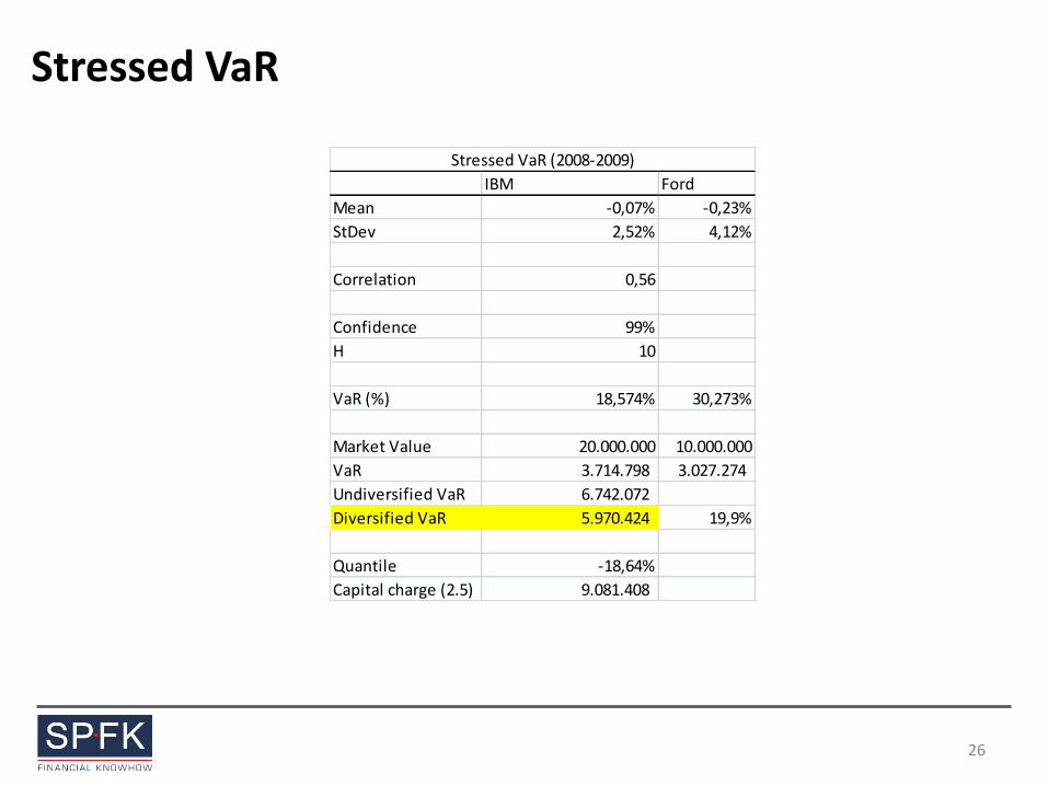
Stressed VaR

IBM Ford

Mean -0,07% -0,23%

StDev 2,52% 4,12%

Correlation 0,56

Confidence 99%

H 10

VaR (%) 18,574% 30,273%

Market Value 20.000.000 10.000.000

VaR 3.714.798 3.027.274

Undiversified VaR 6.742.072

Diversified VaR 5.970.424 19,9%

Quantile -18,64%

Capital charge (2.5) 9.081.408

Stressed VaR (2008-2009)

26

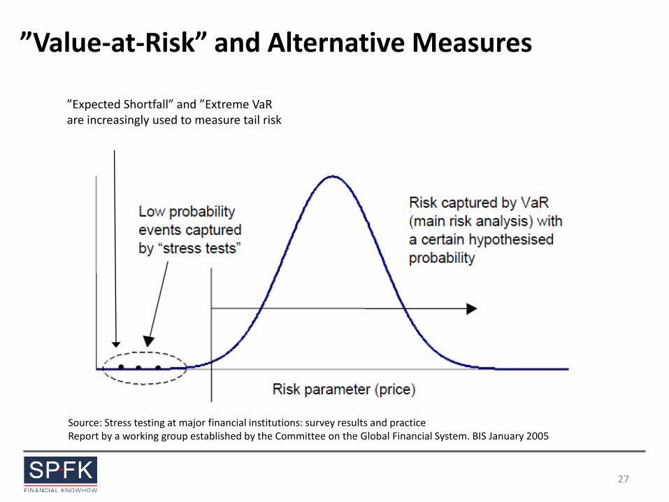
”Value-at-Risk” and Alternative Measures

Source: Stress testing at major financial institutions: survey results and practice Report by a working group established by the Committee on the Global Financial System. BIS January 2005

”Expected Shortfall” and ”Extreme VaR are increasingly used to measure tail risk

27

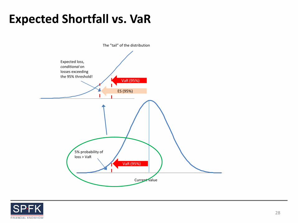
Expected Shortfall vs. VaR

Current value

VaR (95%)

5% probability of loss > VaR

VaR (95%)

ES (95%)

Expected loss, conditional on losses exceeding the 95% threshold!

The ”tail” of the distribution

28

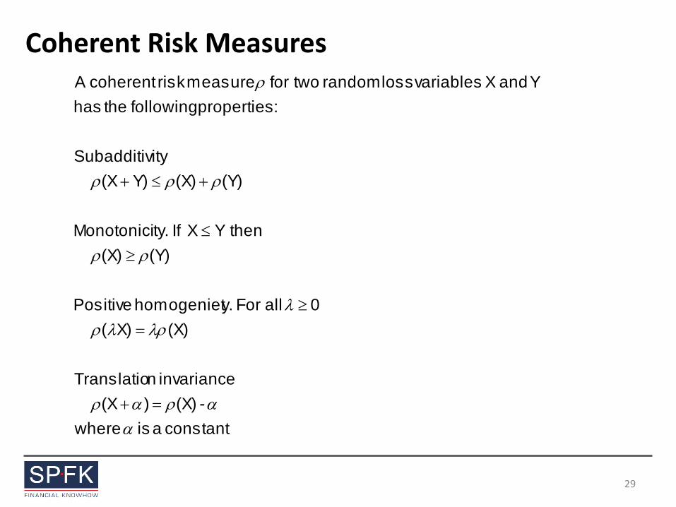
Coherent Risk Measures

constant a is where

-(X))(X

invariance nTranslatio

(X)X)(

0 all For y.homogeniet Positive

(Y)(X)

thenY X If ty.Monotonici

(Y)(X)Y)(X

itySubadditiv

:properties following the has

Y and X variables loss random two for measure risk coherentA

29

Which approaches are coherent?

• VAR measures are not coherent – Not sub-additive

• Expected shortfall (mean excess, tail VAR) is coherent

30

Example

• Two different bonds A and B with non–overlapping default probabilities

• For example: two bonds issued by Nokia and Motorola: If one defaults the other will not and vice versa.

• A portfolio that contains both bonds may have a global VaR which is bigger than the sum of the two VaR’s.

• Numerical example. – The two bonds have two different default states each with recovery values at

70 and 90 and probabilities 3% and 2% respectively.

– Otherwise they will redeem at 100.

31

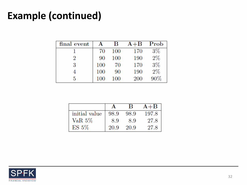
Example (continued)

32

Ways of Calculating ES

• Analytical Metods – Normal distribution

– Extreme VaR (GPD)

• Numerical Methods – Estimate full distribution using

• Historical simulation

• Monte Carlo simulation

33

“Extreme Value Theory”

• Extreme Value Theory (EVT) focuses on estimation of tails of probability distributions

• Two main approaches in EVT – Peaks-over-threshold (POT)

– Block maxima approach

34

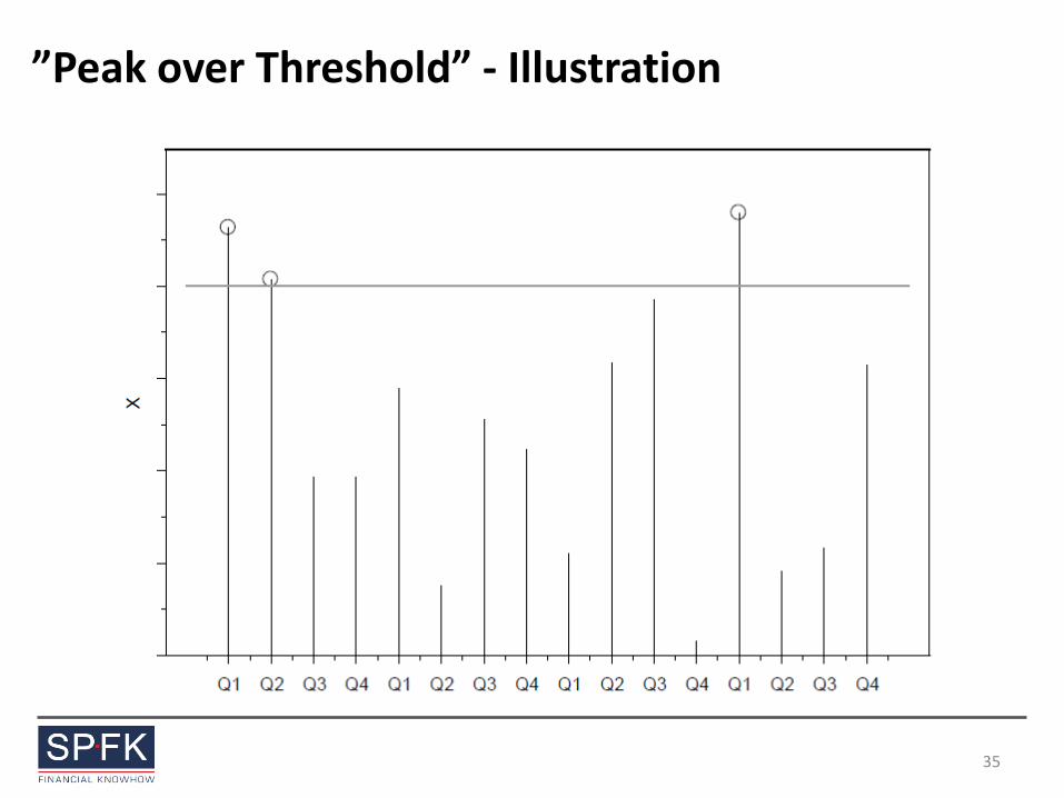
”Peak over Threshold” - Illustration

35

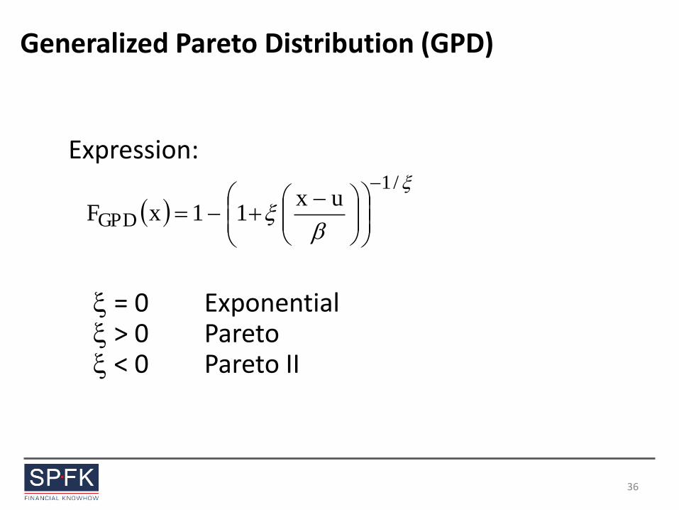
Generalized Pareto Distribution (GPD)

Expression: = 0 Exponential > 0 Pareto < 0 Pareto II

/1

GPDux

11xF

36

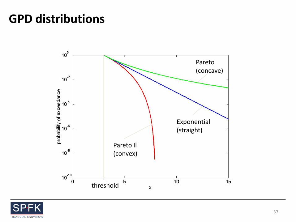
GPD distributions

Pareto (concave)

Exponential (straight)

Pareto Il (convex)

threshold

37

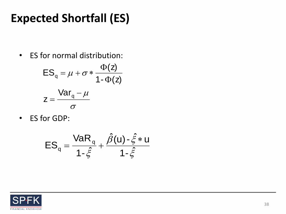
Expected Shortfall (ES)

• ES for normal distribution:

• ES for GDP:

q

q

Varz

z)(-1

z)(ES

ˆ-1

uˆ-(u)ˆ

ˆ-1

VaRES

q

q

38

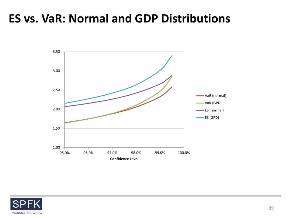
ES vs. VaR: Normal and GDP Distributions

1.00

1.50

2.00

2.50

3.00

3.50

95.0% 96.0% 97.0% 98.0% 99.0% 100.0%

Confidence Level

VaR (normal)

VaR (GPD)

ES (normal)

ES (GPD)

39

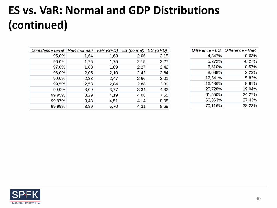
ES vs. VaR: Normal and GDP Distributions (continued)

Confidence Level VaR (normal) VaR (GPD) ES (normal) ES (GPD)

95,0% 1,64 1,63 2,06 2,15

96,0% 1,75 1,75 2,15 2,27

97,0% 1,88 1,89 2,27 2,42

98,0% 2,05 2,10 2,42 2,64

99,0% 2,33 2,47 2,66 3,01

99,5% 2,58 2,84 2,88 3,39

99,9% 3,09 3,77 3,34 4,32

99,95% 3,29 4,19 4,08 7,55

99,97% 3,43 4,51 4,14 8,08

99,99% 3,89 5,70 4,31 8,69

Difference - ES Difference - VaR

4,347% -0,63%

5,272% -0,27%

6,610% 0,57%

8,688% 2,23%

12,541% 5,83%

16,436% 9,91%

25,728% 19,94%

61,550% 24,27%

66,863% 27,43%

70,116% 38,23%

40

Risk-Adjusted Performance Measurement in Banks

41

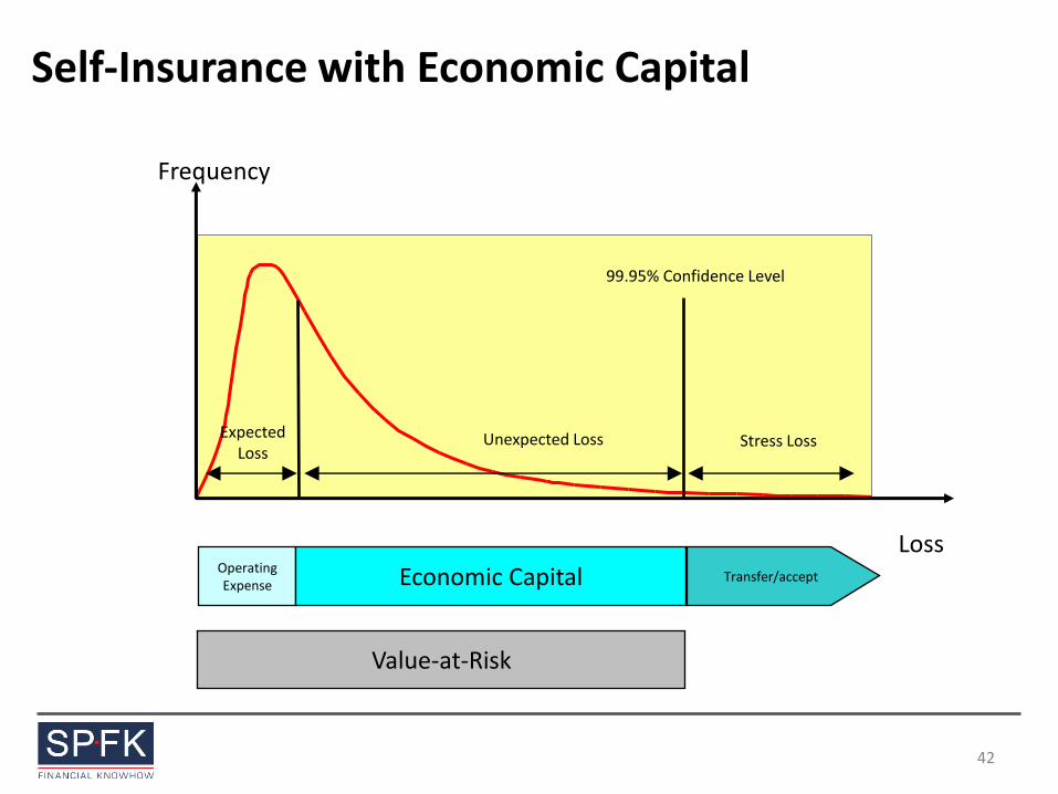
Self-Insurance with Economic Capital

Frequency

Loss

Expected Loss

Unexpected Loss Stress Loss

99.95% Confidence Level

Operating Expense Economic Capital Transfer/accept

Value-at-Risk

42

Optimal Capital Allocation

• Key problem: How to aggregate the risks attributed to the bank’s various business lines

• Some banks choose simply to add risks up and thus recognize none of the benefits of risk diversification

• Others use flat percentage reduction in risk capital to reflect diversification

43

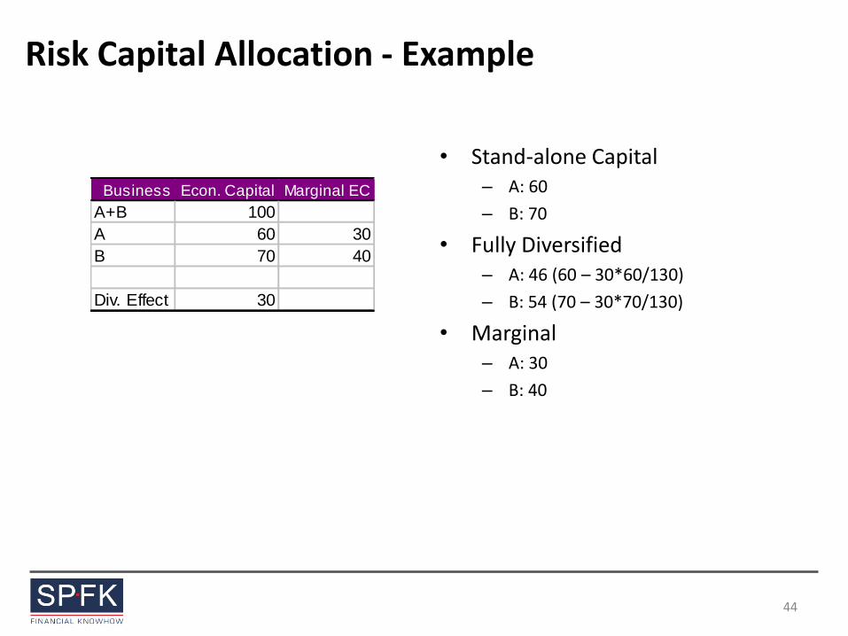
Risk Capital Allocation - Example

• Stand-alone Capital – A: 60

– B: 70

• Fully Diversified – A: 46 (60 – 30*60/130)

– B: 54 (70 – 30*70/130)

• Marginal – A: 30

– B: 40

Business Econ. Capital Marginal EC

A+B 100

A 60 30

B 70 40

Div. Effect 30

44

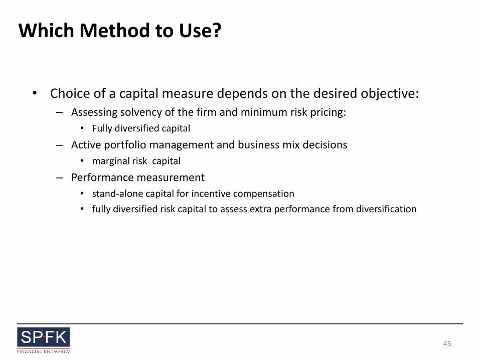
Which Method to Use?

• Choice of a capital measure depends on the desired objective: – Assessing solvency of the firm and minimum risk pricing:

• Fully diversified capital

– Active portfolio management and business mix decisions

• marginal risk capital

– Performance measurement

• stand-alone capital for incentive compensation

• fully diversified risk capital to assess extra performance from diversification

45

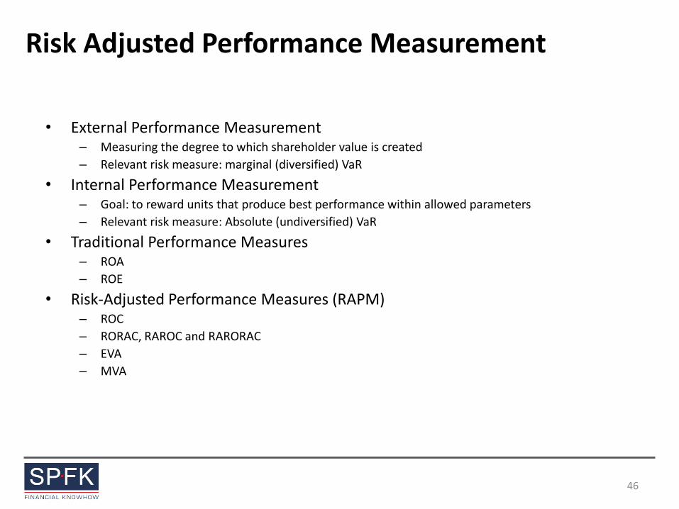
Risk Adjusted Performance Measurement

• External Performance Measurement – Measuring the degree to which shareholder value is created

– Relevant risk measure: marginal (diversified) VaR

• Internal Performance Measurement – Goal: to reward units that produce best performance within allowed parameters

– Relevant risk measure: Absolute (undiversified) VaR

• Traditional Performance Measures – ROA

– ROE

• Risk-Adjusted Performance Measures (RAPM) – ROC

– RORAC, RAROC and RARORAC

– EVA

– MVA

46

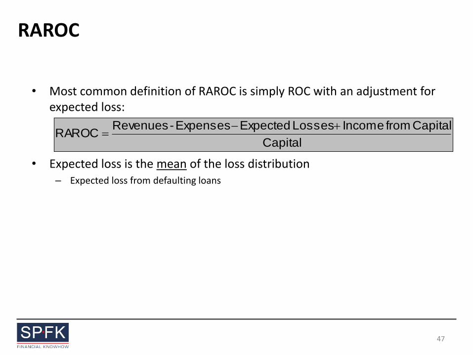
RAROC

• Most common definition of RAROC is simply ROC with an adjustment for expected loss:

• Expected loss is the mean of the loss distribution – Expected loss from defaulting loans

Capital

Capital from Income Losses ExpectedExpenses-RevenuesRAROC

47

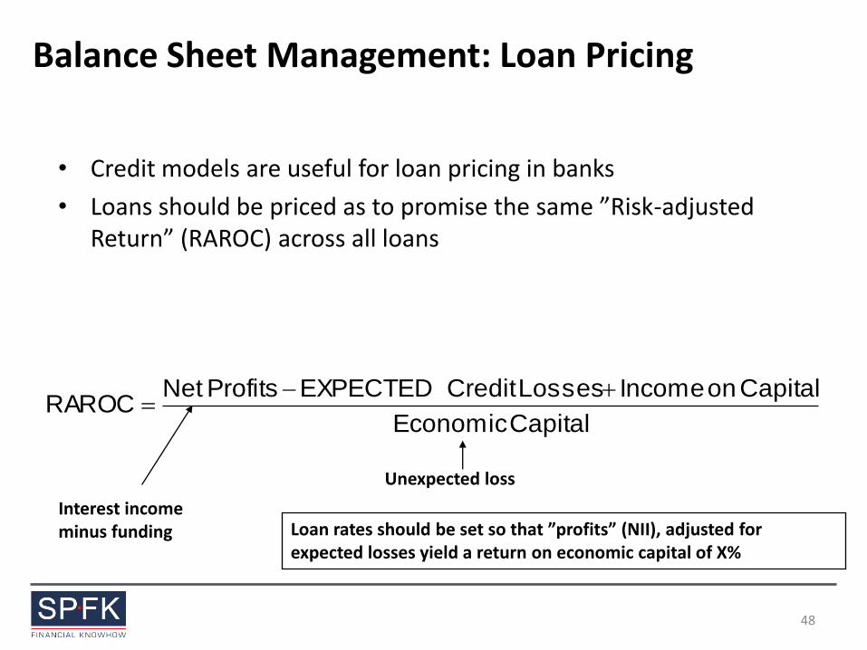
Balance Sheet Management: Loan Pricing

• Credit models are useful for loan pricing in banks

• Loans should be priced as to promise the same ”Risk-adjusted Return” (RAROC) across all loans

CapitalEconomic

Capital on IncomeLosses Credit EXPECTEDProfitsNetRAROC

Loan rates should be set so that ”profits” (NII), adjusted for expected losses yield a return on economic capital of X%

Interest income minus funding

Unexpected loss

48

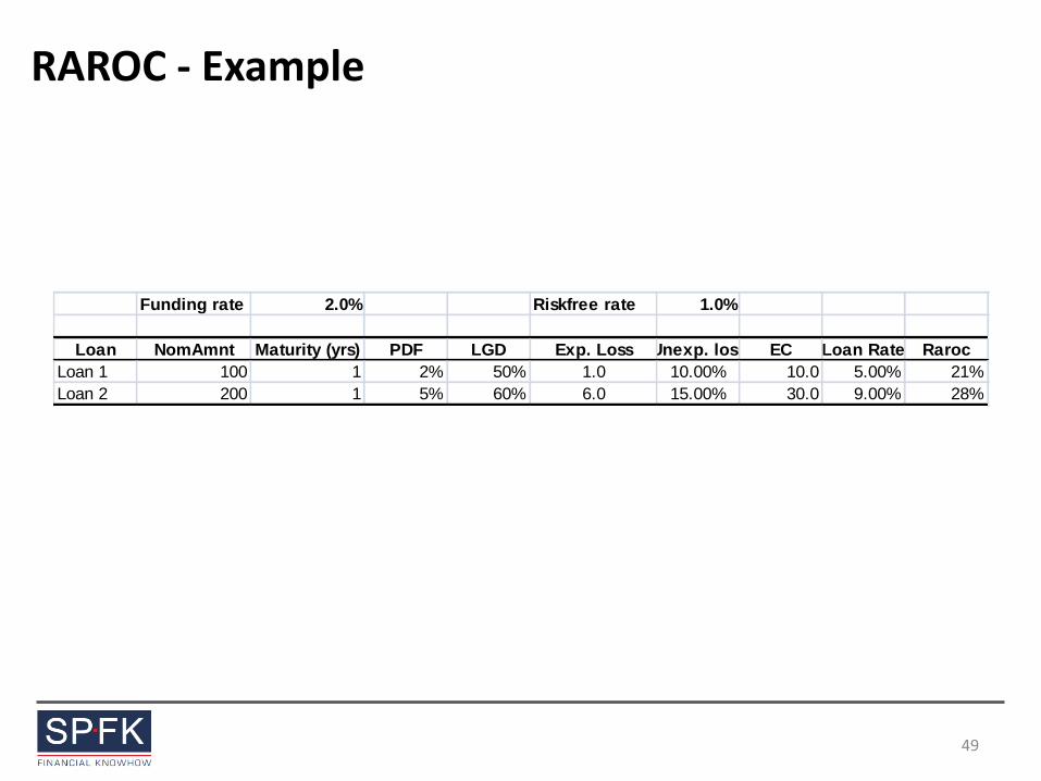
RAROC - Example

49

Funding rate 2.0% Riskfree rate 1.0%

Loan NomAmnt Maturity (yrs) PDF LGD Exp. Loss Unexp. loss EC Loan Rate Raroc

Loan 1 100 1 2% 50% 1.0 10.00% 10.0 5.00% 21%

Loan 2 200 1 5% 60% 6.0 15.00% 30.0 9.00% 28%

Risk-Adjusted Performance Measurement of Investment

Portfolios

50

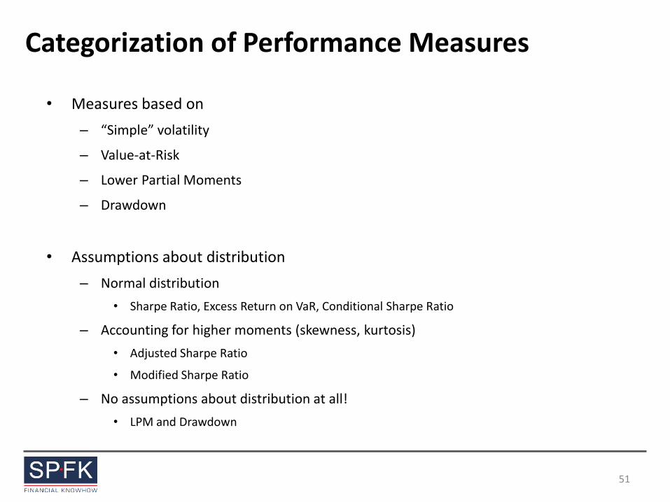
Categorization of Performance Measures

• Measures based on

– “Simple” volatility

– Value-at-Risk

– Lower Partial Moments

– Drawdown

• Assumptions about distribution

– Normal distribution

• Sharpe Ratio, Excess Return on VaR, Conditional Sharpe Ratio

– Accounting for higher moments (skewness, kurtosis)

• Adjusted Sharpe Ratio

• Modified Sharpe Ratio

– No assumptions about distribution at all!

• LPM and Drawdown

51

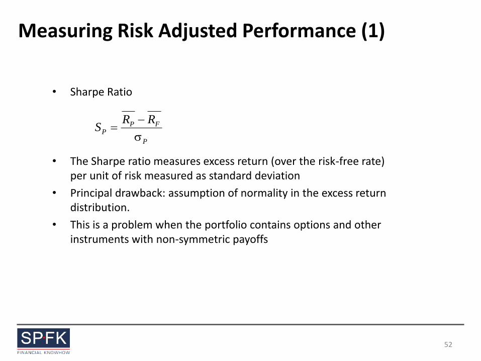
• Sharpe Ratio

• The Sharpe ratio measures excess return (over the risk-free rate) per unit of risk measured as standard deviation

• Principal drawback: assumption of normality in the excess return distribution.

• This is a problem when the portfolio contains options and other instruments with non-symmetric payoffs

Measuring Risk Adjusted Performance (1)

P

FPP

RRS

52

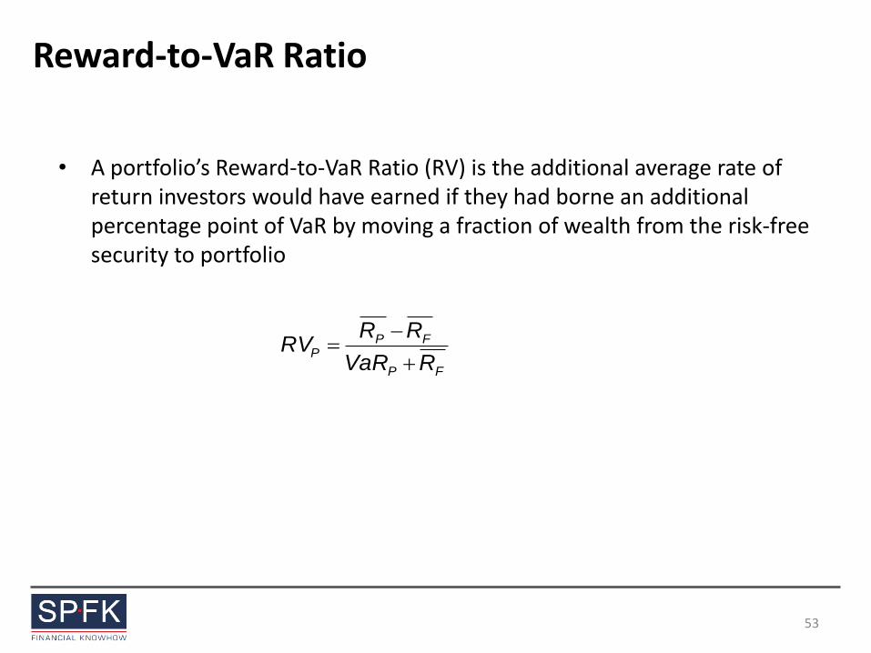
Reward-to-VaR Ratio

• A portfolio’s Reward-to-VaR Ratio (RV) is the additional average rate of return investors would have earned if they had borne an additional percentage point of VaR by moving a fraction of wealth from the risk-free security to portfolio

FP

FPP

RVaR

RRRV

53

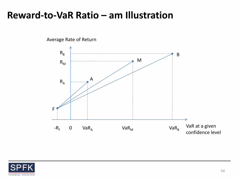
Reward-to-VaR Ratio – am Illustration

F

A

M B

VaRA VaRM VaRB

RA

RM

RB

0 -Rf

Average Rate of Return

VaR at a given confidence level

54

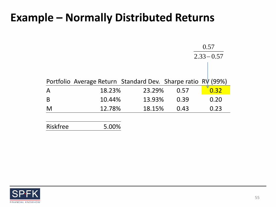
Example – Normally Distributed Returns

57.033.2

57.0

Portfolio Average Return Standard Dev. Sharpe ratio RV (99%)

A 18.23% 23.29% 0.57 0.32

B 10.44% 13.93% 0.39 0.20

M 12.78% 18.15% 0.43 0.23

Riskfree 5.00%

55

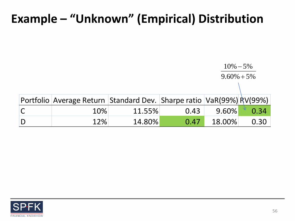
Example – “Unknown” (Empirical) Distribution

Portfolio Average Return Standard Dev. Sharpe ratio VaR(99%) RV(99%)

C 10% 11.55% 0.43 9.60% 0.34

D 12% 14.80% 0.47 18.00% 0.30

%5%60.9

%5%10

56

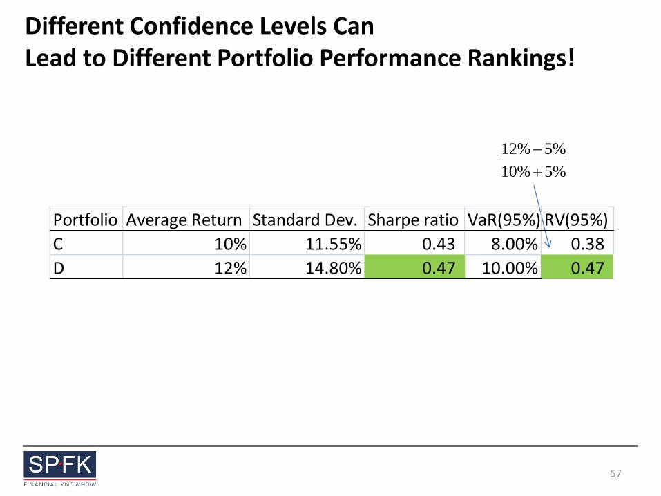
Different Confidence Levels Can Lead to Different Portfolio Performance Rankings!

%5%10

%5%12

Portfolio Average Return Standard Dev. Sharpe ratio VaR(95%) RV(95%)

C 10% 11.55% 0.43 8.00% 0.38

D 12% 14.80% 0.47 10.00% 0.47

57

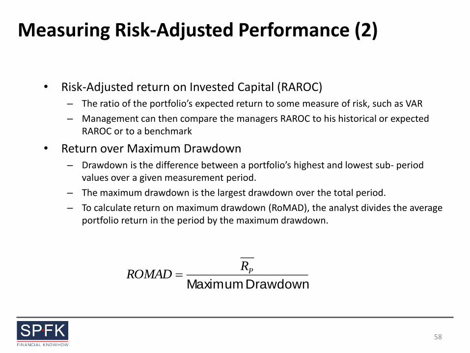
• Risk-Adjusted return on Invested Capital (RAROC) – The ratio of the portfolio’s expected return to some measure of risk, such as VAR

– Management can then compare the managers RAROC to his historical or expected RAROC or to a benchmark

• Return over Maximum Drawdown – Drawdown is the difference between a portfolio’s highest and lowest sub- period

values over a given measurement period.

– The maximum drawdown is the largest drawdown over the total period.

– To calculate return on maximum drawdown (RoMAD), the analyst divides the average portfolio return in the period by the maximum drawdown.

Measuring Risk-Adjusted Performance (2)

Drawdown MaximumPR

ROMAD

58

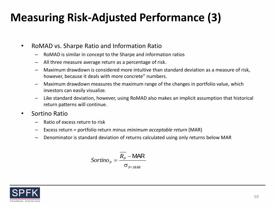
• RoMAD vs. Sharpe Ratio and Information Ratio – RoMAD is similar in concept to the Sharpe and information ratios

– All three measure average return as a percentage of risk.

– Maximum drawdown is considered more intuitive than standard deviation as a measure of risk, however, because it deals with more concrete” numbers.

– Maximum drawdown measures the maximum range of the changes in portfolio value, which investors can easily visualize.

– Like standard deviation, however, using RoMAD also makes an implicit assumption that historical return patterns will continue.

• Sortino Ratio – Ratio of excess return to risk

– Excess return = portfolio return minus minimum acceptable return (MAR)

– Denominator is standard deviation of returns calculated using only returns below MAR

Measuring Risk-Adjusted Performance (3)

MARP

PP

RSortino

MAR

59