Embed Size (px)
Citation preview
University of Rhode Island University of Rhode Island
DigitalCommons@URI DigitalCommons@URI
Open Access Dissertations
2016
Valuation of Unconventional Oil and Gas Development Valuation of Unconventional Oil and Gas Development
Andrew J. Boslett University of Rhode Island, [email protected]
Follow this and additional works at: https://digitalcommons.uri.edu/oa_diss
Recommended Citation Recommended Citation Boslett, Andrew J., "Valuation of Unconventional Oil and Gas Development" (2016). Open Access Dissertations. Paper 474. https://digitalcommons.uri.edu/oa_diss/474
This Dissertation is brought to you for free and open access by DigitalCommons@URI. It has been accepted for inclusion in Open Access Dissertations by an authorized administrator of DigitalCommons@URI. For more information, please contact [email protected].
VALUATION OF UNCONVENTIONAL OIL AND GAS DEVELOPMENT
BY
ANDREW J. BOSLETT
A DISSERTATION SUBMITTED IN PARTIAL FULFILLMENT OF THE
REQUIREMENTS FOR THE DEGREE OF DOCTOR OF PHILOSOPHY
IN
ENVIRONMENTAL AND NATURAL RESOURCE ECONOMICS
UNIVERSITY OF RHODE ISLAND
2016
DOCTOR OF PHILOSOPHY DISSERTATION
OF
ANDREW J. BOSLETT
APPROVED:
DISSERTATION COMMITTEE TODD GUILFOOS
COREY LANG
PETER AUGUST
NASSER H. ZAWIA
DEAN OF GRADUATE SCHOOL
UNIVERSITY OF RHODE ISLAND
2016
ABSTRACT
Valuation of Unconventional Oil and Gas Development
By
Andrew J. Boslett
Doctor of Philosophy of Environmental and Natural Resource Economics
University of Rhode Island
Public discourse regarding the local economic, environmental, and socio-cultural
impacts of unconventional oil and gas development has been intense, especially in those
areas of the country that are relatively unfamiliar with extractive industry. At the center
of this debate is the contrast between the economic and financial benefits that accrue to
local governments and landowners versus the environmental and socio-cultural costs
borne by the public-at-large. Understanding how local citizens value unconventional oil
and gas development is an important policy consideration for federal, state, and local
governments.
The overarching theme of this work, consisting of three manuscripts, seeks to
contribute to the debate regarding the impacts of energy consumption and development. In
two manuscripts, I use the hedonic valuation approach to value the benefits and costs of
shale gas and oil development. I do this through the context of a statewide moratorium on
development in New York and a long-standing severance between the surface and mineral
estates in the western Colorado property market.
My results indicate that homebuyers significantly value both the financial benefits
and environmental costs of unconventional oil and gas development. In Manuscript 1, I
find that New York properties that were most likely to experience the financial and
environmental impacts of Marcellus Shale development decreased in value by 23% as a
result of the moratorium, which under certain assumptions indicates a large and positive
net valuation of development. In Manuscript 2, I find that the homebuyers have large
and significant valuations of the environmental costs of development on the order of
35% of sale prices for those properties that have an unconventional well within a mile
of the property’s extent.
In my third manuscript, I again apply hedonic valuation and value the benefits and
costs of silica sand mining in western Wisconsin. The great increase in the application of
hydraulic fracturing in oil and gas production has led to an increase in demand for silica
sand. This type of sand is an important ingredient in hydraulic fracturing. Silica sand
mining has a number of local benefits and external costs. I use the hedonic valuation
methodology to value sand mining’s impacts, focusing on property views and local air
quality. I find strong evidence that both changes in view and air quality are negatively
capitalized into housing prices. I also find evidence of appreciation for those properties
that are not as subject to those environmental quality changes.

iv
ACKNOWLEDGEMENTS
The last four years have been a time of both personal and professional
development. I’d like to make some acknowledgements.
I am very grateful for the guidance, honesty, and patience of my adviser, Todd
Guilfoos. He encouraged me to pursue my research interests, every step of the way.
During our conversations, he gave me insights on what it means to be both an economist
and professional. I’ve enjoyed working with him and I appreciate the time we’ve worked
together.
I would also like to thank other faculty and staff at URI: Corey Lang, for his
teachings in applied econometrics and for our collaborations; Peter August, for his
helpful videos on ArcGIS and his open-door policy with related-questions; Jim Opaluch,
for helpful dialogue about economics throughout my time at URI (especially towards the
end); Stephen Atlas, for inviting me into his lab group and giving me insights on
behavioral economics and mental processing; Professor Emi Uchida, for bringing me
here to Rhode Island, for funding me for my first three years in the program as part of her
ecosystem services project in Rhode Island, and for many helpful conversations along the
way; Professor Tom Sproul, for many interesting conversations and for first encouraging
me to think about problems from an experimental framework; and Denise Foley and Judy
Palmer, for their help and patience over the last four years.
I’d like to thank Claudia Hitaj and Jeremy Weber for taking me on as an intern at
the USDA’s Economic Research Service. It was a great experience. I’d also like to thank
Professor Karin Limburg from the SUNY College of Environmental Science and
Forestry, for her encouragement and advice on research and life, and Sam Piel of

v
Hanover Engineering, for teaching me a lot about GIS, which has been my comparative
advantage.
I have been fortunate to become friends with many of my colleagues over the last
four years, especially Pam Booth, Robert Dinterman, Brandon Elsner, Carrie Gill,
Tingting Liu, Nate Merrill, and Edson Okwelum. I’d also like to thank India and Sprout
for their constant support and affection.
Words cannot express my appreciation to my Mom and Dad. Every day I am
reminded of how blessed I am to be their son. They have supported in every area of my
life.
Same goes for my brother, Jim. Our bike tours over the last couple years have
been a great inspiration. Here’s to many more, especially after my latest incentive…
I’d like to thank my loving wife, Lindsay. You’ve built me up every day since
I’ve met you. I can’t thank you enough for everything you’ve done for me. Your belief in
me has made the difference.
Last but not least, I should thank the State of Rhode Island and the USDA for
funding my time here in Rhode Island.
vi
PREFACE
This dissertation is written in three-manuscript form. The first manuscript is co-
authored with Todd Guilfoos and Corey Lang. It has been published in the Journal of
Environmental Economics and Management. The second manuscript is also co-authored
with Todd Guilfoos and Corey Lang. It is in review at the Journal of the Association of
Environmental and Resource Economists. The third manuscript is solo-authored and is
being prepared to submit to Land Economics or Resource and Energy Economics.
Manuscript 1: Valuation of Expectations: A Hedonic Study of Shale Gas Development
and New York’s Moratorium
Manuscript 2: Valuation of the External Costs of Unconventional Oil and Gas
Development: The Critical Importance of Mineral Rights Ownership
Manuscript 3: A Bucket or a Sieve? A Valuation of Views and Air Quality around Silica
Sand Mining in Wisconsin
vii
TABLE OF CONTENTS
ABSTRACT ........................................................................................................................ ii
ACKNOWLEDGEMENTS ............................................................................................... iv
PREFACE .......................................................................................................................... vi
TABLE OF CONTENTS .................................................................................................. vii
LIST OF FIGURES ............................................................................................................ x
LIST OF TABLES ............................................................................................................. xi
Manuscript – 1 .................................................................................................................... 1
Abstract ........................................................................................................................... 2
1. Introduction ................................................................................................................. 3
2. Background ................................................................................................................. 9
3. Conceptual Framework ............................................................................................ 15
4. Methodology ............................................................................................................. 19
5. Data ........................................................................................................................... 23
6. Results ....................................................................................................................... 27
7. Conclusion ................................................................................................................ 35
References ..................................................................................................................... 37
Tables and Figures ........................................................................................................ 43
Appendix ....................................................................................................................... 52
viii
Manuscript – 2 .................................................................................................................. 76
Abstract ......................................................................................................................... 77
1. Introduction ............................................................................................................... 78
2. Conceptual Framework ............................................................................................. 82
3. The Stock-Raising Homestead Act of 1916 .............................................................. 84
4. Empirical Setting and Data ....................................................................................... 88
5. Methodology ............................................................................................................. 91
5. Results ....................................................................................................................... 96
6. Conclusion ............................................................................................................... 102
References ................................................................................................................... 104
Tables & Figures ......................................................................................................... 110
Appendix ..................................................................................................................... 120
Manuscript – 3 ................................................................................................................ 132
Abstract ....................................................................................................................... 133
1. Introduction ............................................................................................................. 134
2. Background ............................................................................................................. 140
3. Data ......................................................................................................................... 143
4. Methodology ........................................................................................................... 146
5. Results ..................................................................................................................... 154
6. Conclusions ............................................................................................................. 161
ix
References ................................................................................................................... 164
Tables and Figures ...................................................................................................... 168
Technical Appendix ........................................................................................................ 179
First Stage of Hedonic Valuation ................................................................................ 179
Second Stage of Hedonic Valuation............................................................................ 186
References ................................................................................................................... 190
Tables & Figures ......................................................................................................... 191
x
LIST OF FIGURES
Manuscript 1
Figure 1: Timeline of New York policies on shale gas development and the number of
wells drilled in Pennsylvania from 2006 to 2014 .......................................................43
Figure 2: Unconventional well development in Bradford and Tioga counties from 2006 to
2011 ............................................................................................................................44
Figure 3: Shale thickness and border restrictions across sample counties .........................45
Figure 4: Pre-moratorium sale price trends .......................................................................46
Figure A1: Household movement across the NY-PA border ............................................59
Figure A2: Observed transactions from 2006 to 2011 in sample counties ........................60
Figure A3: New York townships that have passed pre-emptive resolutions in support of
shale gas development ................................................................................................61
Figure A4: Shale depth and border restrictions across our study area counties ................62
Manuscript 2
Figure 1: Map of unconventional oil and gas development in Colorado .........................116
Figure 2: Map of Western Colorado ................................................................................117
Figure 3: Distance bin parameter estimates and histogram of well distance ...................118
Figure 4: Propensity score distributions for one mile treatment, pre versus post matching
(Nearest Neighbor 3 – 1) ..........................................................................................119
Figure 1A: Close-up view of unconventional well development in southern Garfield
County and northwestern Mesa County ...................................................................131
Manuscript 3
Figure 1: Silica sand regions in Wisconsin ......................................................................176
Figure 2: Study area in western Wisconsin......................................................................177
Figure 3: Silica sand mining buffers ................................................................................178
Technical Appendix
Figure 1: Joint envelope of bid and offer functions .........................................................191
xi
LIST OF TABLES
Manuscript 1
Table 1: Summary statistics ...............................................................................................47
Table 2: Double difference estimates of the impact of the NY shale gas development
moratorium on housing prices ....................................................................................48
Table 3: Robustness checks for the 5 mile border restriction and shale thickness model .49
Table 4: Heterogeneous impacts of the moratorium by acreage and for resolution towns 50
Table 5: Impact of unconventional well density on residential property prices in
Pennsylvania ...............................................................................................................51
Table A1: A review of potential landowner monetary benefits from shale gas
development................................................................................................................63
Table A2: A review of potential environmental impacts of shale gas development .........65
Table A3: Summary statistics ............................................................................................66
Table A4 - Demographic, Economic, and Social Characteristics ......................................67
Table A5: Robustness checks (5 mile border & shale trim restrictions) ...........................68
Table A6: Comprehensive results from Table 2 ................................................................69
Table A7: Double difference estimates of the impact of the NY shale gas development
moratorium on housing prices, Linear Model ............................................................70
Table A8: Robustness checks for the 5 mile border restriction and shale thickness
model ..........................................................................................................................71
Table A9: Robustness checks for the 15 mile border restriction and shale thickness
model ..........................................................................................................................72
Table A10: The effect of local resolutions in support of SGD on housing prices .............73
Manuscript 2
Table 1: Financial benefits and environmental costs of oil and gas development,
differentiated by mineral estate ownership classification .........................................110
Table 2: Summary statistics .............................................................................................111
Table 3: The effect of unconventional development on residential properties with federal
mineral ownership ....................................................................................................112
xii
Table 4: Robustness checks .............................................................................................113
Table 5: The effect of unconventional development on split estate properties using
matching techniques .................................................................................................114
Table 6: The effect of unconventional development on all residential properties (N =
47,139), binary treatment ..........................................................................................115
Table 1A: Mineral rights ownership in the previous literature on unconventional oil and
gas development .......................................................................................................123
Table 2A: Comprehensive results of our models from Table 3 in the main text .............124
Table 3A: The effect of unconventional development on the residential properties with
federal mineral ownership, count treatment .............................................................126
Table 4A: The effect of unconventional development on the residential properties with
federal mineral ownership in levels of sale price .....................................................127
Table 5A: Additional robustness checks..........................................................................128
Table 6A: Pre and post-matching statistics ......................................................................129
Table 7A: The effect of unconventional development on all residential properties (N =
47,139), continuous treatment ..................................................................................130
Manuscript 3
Table 1: Summary statistics .............................................................................................168
Table 2: Impact of silica sand mining on nearby residential property prices ..................169
Table 3: Additional robustness checks ............................................................................170
Table 4: Impact of silica sand mining on nearby residential property prices, by
visibility ....................................................................................................................171
Table 5: Alternative visibility approach using r-mile buffers ..........................................172
Table 6: Impact of silica sand mining on nearby residential property prices, by cardinal
direction ....................................................................................................................173
Table 7: Impact of silica sand mining on nearby residential property prices, by view and
cardinal direction ......................................................................................................174
Table 8: Robustness checks for four mile buffer models ................................................175
1
Manuscript – 1
Published in Journal of Environmental Economics and Management, May 2016
Valuation of Expectations:
A Hedonic Study of Shale Gas Development and New York’s Moratorium
Andrew Boslett, Todd Guilfoos, and Corey Lang
Environmental and Natural Resource Economics, University of Rhode Island
2
Abstract
This paper examines the local impacts of shale gas development (SGD). We use a
hedonic framework and exploit a discrete change in expectations about SGD caused by
the New York State moratorium on hydraulic fracturing. Our research design combines
difference-in-differences and border discontinuity, as well as underlying shale geology,
on properties in Pennsylvania and New York. Results suggest that New York properties
that were most likely to experience both the financial benefits and environmental
consequences of SGD dropped in value 23% as a result of the moratorium, which under
certain assumptions indicates a large and positive net valuation of SGD.
Keywords: shale gas development; hydraulic fracturing; hedonic valuation; expectations;
rational expectations; moratorium; difference-in-differences; border discontinuity
3
1. INTRODUCTION
Shale gas development (SGD) has dramatically changed the US energy landscape
in the last decade. The Energy Information Administration (2013) predicts that the US
will shift from being a net importer to a net exporter of natural gas by 2020 and domestic
production will increase 44% by 2040. Much of the attention on SGD has been on the
Marcellus Shale, which extends over 95,000 square miles across New York, Ohio,
Pennsylvania, and West Virginia (Kargbo et al., 2010). Marcellus drilling began in 2005
and has been the source of considerable extraction. From 2005 to 2014, 7,797
unconventional wells have been drilled in Pennsylvania alone.
While the macroeconomic benefits to the US economy are clear, there is
uncertainty surrounding the local benefits and costs to households and communities
impacted by SGD. Property owners with mineral rights can receive substantial gas lease
and production royalties (Pennsylvania Department of Environmental Protection, 2012);
however, little is known about the magnitude of payments due to the private nature of the
contracts. Potential costs of SGD could include various health and environmental impacts
such as water pollution, air pollution, and traffic congestion. The impacts from the health
and environmental externalities are also highly uncertain.
Given the current scale of SGD and expected growth in the future, it is critical to
understand to the local valuation of SGD. This paper seeks to answer this question
using a hedonic framework, as housing prices should reflect the future stream of
benefits and costs tied to the property. Empirically, this is hindered in two ways. First,
the location of wells may be endogenous. Second, expectations about SGD form in
advance of actual drilling, and if expectations are capitalized into housing prices, then a
4
simple before-after comparison may lead to incorrect inference about the valuation. We
mitigate these confounding factors by specifically focusing on expectations and using
an exogenous shift in expectations to reveal valuation.
Just as hydraulic fracturing was beginning its exponential increase in
Pennsylvania, New York State implemented a de facto moratorium on hydraulic
fracturing on July 23, 2008, citing uncertainty about health and environmental impacts
(State of New York's Executive Chamber, 2008).1 The state extended the moratorium
multiple times between 2010 and 2014 (e.g., Wiessner, 2011) and, on December 17,
2014, the New York Department of Environmental Conservation implemented a
permanent ban (Kaplan, 2014). These decisions were highly contentious, as evidenced by
several dozen towns in New York passing resolutions in support of SGD in the spring
and summer of 2012 and 15 towns are currently considering secession (Mathias, 2015).2
To date, there has been no hydraulic fracturing in New York.
This paper exploits changes in expectations that resulted from New York’s
moratorium on drilling and measures this event’s impact on housing prices. Importantly,
the moratorium did not mark a change in the amount of hydraulic fracturing in New York
– expectations about future SGD are the only thing that changed.
We estimate the effect of the statewide moratorium using a difference-in-
differences methodology. We use Pennsylvania as a counterfactual because
1 There is considerable heterogeneity in state regulation on shale gas development as a result of different
political, hydrological, and geological dynamics (Kulander, 2013; Richardson et al., 2013). Some states
have used a more lenient approach to regulation. For example, Pennsylvania had no specific regulations
concerning hydraulic fracturing until early 2010 (Kulander, 2013). Since then, Governor Tom Corbett’s
signed Act 13, prohibiting any local regulation or restrictions on shale gas well production (Begos, 2012).
Like New York, New Jersey and Maryland have enacted regulations to restrict or ban hydraulic fracturing. 2 These resolutions could not supersede state law, but were meant to send a signal to state politicians in
Albany and were in contrast to the more common local bans and moratoria implemented elsewhere in the
state.
5
expectations about future SGD were likely similar to those in pre-moratorium New
York, but in contrast with New York, those expectations were realized. Our aim is to
identify the change in prices for properties in New York that are most likely to be
impacted by SGD (both positively and negatively), relative to price changes for similar
properties in Pennsylvania. We use private well water use as a proxy for properties
likely to experience SGD.3 These are essentially rural properties outside of municipal
water supply boundaries, meaning they have the space requirements for drilling.
Further, contaminated well water is one of the most common and serious environmental
costs.
The design of our preferred sample is motivated by a border discontinuity and
underlying shale geology. We begin with property transactions data for two
Pennsylvania and three New York counties along the border. In the vein of recent
border discontinuity designs (e.g., Grout et al., 2011; Turner et al., 2014) and
specifically those that use state borders (Holmes, 1998; Rohlin et al., 2014), we restrict
observations to be within five miles of the border in order to minimize unobserved
differences in price determinants and best model the counterfactual for New York
residents. Even after these restrictions, there are still substantial shale geology
differences across the border. Thus, we further restrict observations to be in a specific
band of shale thickness, a geological characteristic that strongly affects the amount of
gas or oil in a reservoir (Advanced Resources International, 2013). These restrictions
are meant to improve the similarity of expectations about future SGD. Post-moratorium
spillovers across the border are a threat to identification. However, we contend that
3 While we cannot predict exactly where SGD would occur in New York, 99.8% of drilling in our
Pennsylvania sample occurred in private well water areas.
6
these effects are minimal due to pre-moratorium expectations about spillovers, the rapid
pace of drilling stemming from high initial prices, the area comprising a single labor
market, and southerly flow of surface water.
Using the 5-mile border and shale geology restrictions, our results suggest that the
statewide moratorium decreased New York property values 23.1% for those properties
most likely to experience SGD. Relaxing the sample restrictions leads to smaller
estimates in the range of 10-21%, which suggests that effects are heterogeneous across
our New York counties and that accounting for shale geology is critical for understanding
expectations. We estimate a series of robustness checks that test additional shale geology
restrictions, test for spillover effects across the state border, and use municipal water
properties as an additional control, and results are consistent with point estimates in the
range of an 18-26% drop in housing values.
We interpret these results as a positive net valuation of SGD by buyers and sellers
in New York and Pennsylvania. However, this interpretation relies on two assumptions:
the expected probability of SGD in pre-moratorium New York is 1 and the expected
probability of post-moratorium SGD is 0 and New York and Pennsylvania property
owners and buyers accurately valued the negative and positive aspects of SGD prior to
the moratorium. We estimate several models that bolster our confidence in these
assumptions. However, if either of these assumptions are false, we are still recovering the
effect of the moratorium on property values, which is driven by expectations over
financial benefits and environmental externalities of SGD, and this is an important
estimate for areas considering bans on hydraulic fracturing. Further, the estimates serve
as a validation that expectations are capitalized into property values.
7
One of the models we use to test the assumptions needed for an interpretation of
net valuation is a more traditional model of the effect of proximity to drilling using only
our Pennsylvania observations. The results suggest no price impacts of proximity. While
one interpretation is that the impacts of drilling are small, we interpret this to mean that
ex ante expectations established in the initial expansion of SGD in Pennsylvania were
capitalized into property values and were accurate ex post leading property values not to
change. These results corroborate our claim that New York households near the border
have accurate expectations about SGD, which in turn supports a rational expectations
assumption in hedonic valuation.
There are two major contributions of this paper. First, we provide new evidence
of local impacts of SGD. Existing hedonic studies (Gopalakrishnan and Klaiber, 2014;
Muehlenbachs et al., 2014) find negative impacts of nearby drilling for well-water
dependent properties as large as -22%. However, Gopalakrishnan and Klaiber (2014)
also find that negative effects dissipate to a statistical zero 6-12 months after a permit is
issued. Our results lead to very different conclusions. One reason may be that both of
these studies either use data exclusively from western Pennsylvania or derive most of
their identifying variation from western Pennsylvania. A concern is that split estates,
where mineral rights are sold separately from the property, are common in western
Pennsylvania due to the area’s more extensive history of resource extraction (Kelsey et
al., 2012). In contrast, split estates are relatively uncommon in our focus area of eastern
Pennsylvania and south-central New York. Thus, our data are more likely to recover net
effects of SGD because property owners hold mineral rights and will benefit from
royalties and lease payments. Our interpretation of Gopalakrishnan and Klaiber (2014)
8
and Muehlenbachs et al. (2014) is that their estimates capture the negative externality of
SGD near private well water, which is critical to understand, but mostly exclude the
financial benefits because of the area of study. Consistent with this interpretation are
recent survey findings that indicate a majority of property owners that do not hold the
mineral rights to their property are dissatisfied with local drilling, whereas a majority of
property owners holding mineral rights are satisfied (Collins and Nkansah, 2013).4
While the split estate issue is perhaps the most critical, there are other
differences between our study and others that could lead to different estimates of the
local impact of SGD. We incorporate physical attributes of shale geology into the
analysis, which existing valuation studies have not utilized. This appears to be
important to creating valid counterfactuals in a difference-in-differences framework.
Further, our treatment group has no direct experience with SGD, though they seemingly
would learn about it as SGD expanded right across the border. Additionally, we are
estimating area-level impacts that capture impacts occurring to whole areas, as opposed
to a proximity analysis that captures differential impacts for properties nearby drilling.
This focus may average away some of the negative effects of SGD if property owners
in NY expect that they would be minimally impacted by negative externalities since the
placement of future shale gas wells is unknown.
The second contribution is to add to our understanding of how expectations are
capitalized into property values. While many hedonic papers implicitly assume
expectations exist and recent structural models have incorporated expectations (e.g.,
Bishop and Murphy, 2011; Ma, 2013), we offer a particularly clean, reduced-form
4 A survey by Brasier et al. (2013) found that landowners that hold their property’s underlying mineral
rights have generally lower risk perceptions of SGD.
9
illustration of how expectations factor into prices. The effect of the New York
moratorium is to change expectations, whereas the results of the proximity analysis using
only Pennsylvania properties support the idea of rational expectations because no price
changes occur once drilling commences. This work also complements hedonic studies
that show new information can cause capitalization of dis-amenities, even when levels of
dis-amenities do not change (e.g., Pope, 2008; Guignet, 2013).
2. BACKGROUND
The first objective of this section is to catalog various estimates of benefits and
costs of SGD, which is critical for putting our estimates of the net valuation of SGD in
context. Given the private and dispersed nature of financial benefits, it is a contribution of
this paper to compile these estimates. The second objective is to give a timeline of SGD
in Pennsylvania and SGD regulation in New York.
2.1 Financial benefits
During shale gas extraction, owners of sub-surface mineral rights may sign a
mineral lease contract with energy production companies, granting them the right to
develop mineral deposits underneath their property (Pennsylvania Department of
Environmental Protection, 2012). The two primary monetary benefits associated with
shale gas production are lease signing bonuses and royalty payments. A lease signing
bonus is an initial payment, based on acreage, for signing a gas lease contract (Weidner,
2013). Due to the uncertainty of natural gas production, this is perhaps the most
important element of the lease (Hefley et al., 2011). The payment level is based on a
10
number of variables, including geological factors, landowner-stipulated restrictions,
nearby drilling results, and the current state of the natural gas market (Weidner, 2013).
The average per acre signing bonus is $2,700 (Hefley et al., 2011), though this can vary
from $50 to almost $6,000 (Humphries, 2008; Green, 2010; Eichler, 2013; Rieley, 2014).
The other major monetary benefit is royalty payments, which are recurring
payments on a proportion of natural gas production. The minimum royalty rate, set by
law, is 12.5% of the value of extracted natural gas (Pennsylvania Department of
Environmental Protection, 2012). However, the negotiated rate can be much higher,
depending on the same factors that determine lease payments (Weidner, 2013).
According to a Penn State University Extension associate, Marcellus Shale gas
production has generated a cumulative total of $160 million in royalties for landowners in
Bradford County, Pennsylvania as of late 2012 (Loewenstein, 2012).
SGD infrastructure-related benefits can also serve as economic windfalls for
landowners. Surface rights owners can receive monetary payments for allowing pipeline,
compressor station, and water impoundment construction on their properties. These are
often one-time payments. A payment for pipeline easement construction is based on the
length of the constructed pipeline and can range from $5-25 per linear foot (Messersmith,
2010). Due to the nuisance factor associated with compressor stations (e.g., Litovitz et
al., 2013), payments for their construction can range from hundreds of thousands to
millions of dollars (Clark, 2014). Payments for water impoundment construction can
range from $40,000-70,000, but could potentially be lower or higher given their intended
size and permanency (Clark, 2014).
Lastly, governments have the ability to raise revenue through taxing shale gas
11
development, which in turn would have public finance implications. These public
finance measures could then be capitalized in housing prices through improvements to
public goods and services in local municipalities, such as schools. Pennsylvania did
enact an “impact fee” in 2012 through Act 13, retroactive to 2011 activity, which
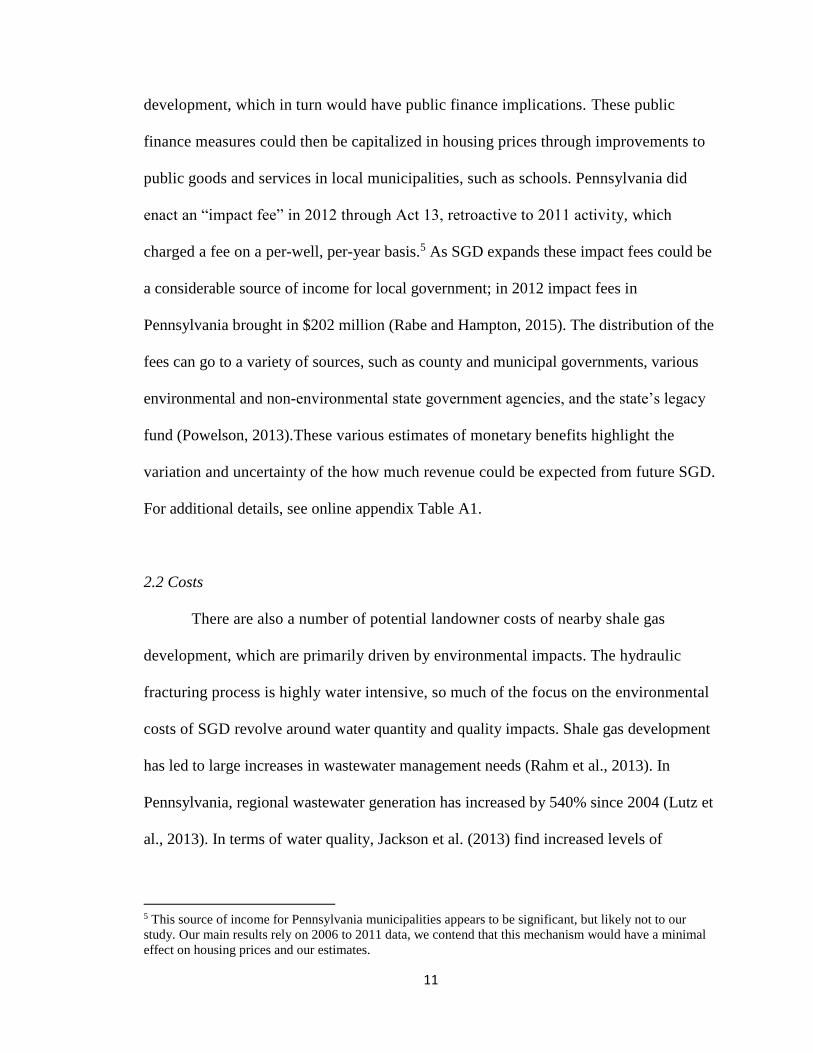
charged a fee on a per-well, per-year basis.5 As SGD expands these impact fees could be
a considerable source of income for local government; in 2012 impact fees in
Pennsylvania brought in $202 million (Rabe and Hampton, 2015). The distribution of the
fees can go to a variety of sources, such as county and municipal governments, various
environmental and non-environmental state government agencies, and the state’s legacy
fund (Powelson, 2013).These various estimates of monetary benefits highlight the
variation and uncertainty of the how much revenue could be expected from future SGD.
For additional details, see online appendix Table A1.
2.2 Costs
There are also a number of potential landowner costs of nearby shale gas
development, which are primarily driven by environmental impacts. The hydraulic
fracturing process is highly water intensive, so much of the focus on the environmental
costs of SGD revolve around water quantity and quality impacts. Shale gas development
has led to large increases in wastewater management needs (Rahm et al., 2013). In
Pennsylvania, regional wastewater generation has increased by 540% since 2004 (Lutz et
al., 2013). In terms of water quality, Jackson et al. (2013) find increased levels of
5 This source of income for Pennsylvania municipalities appears to be significant, but likely not to our
study. Our main results rely on 2006 to 2011 data, we contend that this mechanism would have a minimal
effect on housing prices and our estimates.
12
methane contamination in groundwater in heavy-SGD areas, while Olmstead et al. (2013)
find evidence of surface water pollution as a result of SGD waste disposal and
management processes. In 2014, the Pennsylvania Department of Environmental
Protection released a list of more than 250 instances where SGD operations impacted
water quality in the state.
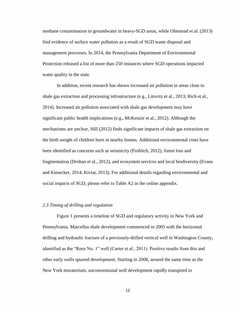
In addition, recent research has shown increased air pollution in areas close to
shale gas extraction and processing infrastructure (e.g., Litovitz et al., 2013; Rich et al.,
2014). Increased air pollution associated with shale gas development may have
significant public health implications (e.g., McKenzie et al., 2012). Although the
mechanisms are unclear, Hill (2012) finds significant impacts of shale gas extraction on
the birth weight of children born in nearby homes. Additional environmental costs have
been identified as concerns such as seismicity (Frohlich, 2012), forest loss and
fragmentation (Drohan et al., 2012), and ecosystem services and local biodiversity (Evans
and Kiesecker, 2014; Kiviat, 2013). For additional details regarding environmental and
social impacts of SGD, please refer to Table A2 in the online appendix.
2.3 Timing of drilling and regulation
Figure 1 presents a timeline of SGD and regulatory activity in New York and
Pennsylvania. Marcellus shale development commenced in 2005 with the horizontal
drilling and hydraulic fracture of a previously-drilled vertical well in Washington County,
identified as the “Renz No. 1” well (Carter et al., 2011). Positive results from this and
other early wells spurred development. Starting in 2008, around the same time as the
New York moratorium, unconventional well development rapidly transpired in
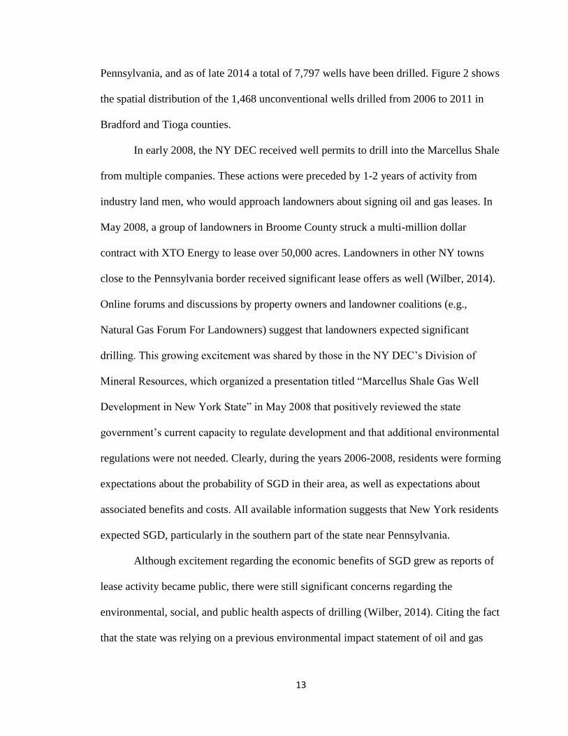
13
Pennsylvania, and as of late 2014 a total of 7,797 wells have been drilled. Figure 2 shows
the spatial distribution of the 1,468 unconventional wells drilled from 2006 to 2011 in
Bradford and Tioga counties.
In early 2008, the NY DEC received well permits to drill into the Marcellus Shale
from multiple companies. These actions were preceded by 1-2 years of activity from
industry land men, who would approach landowners about signing oil and gas leases. In
May 2008, a group of landowners in Broome County struck a multi-million dollar
contract with XTO Energy to lease over 50,000 acres. Landowners in other NY towns
close to the Pennsylvania border received significant lease offers as well (Wilber, 2014).
Online forums and discussions by property owners and landowner coalitions (e.g.,
Natural Gas Forum For Landowners) suggest that landowners expected significant
drilling. This growing excitement was shared by those in the NY DEC’s Division of
Mineral Resources, which organized a presentation titled “Marcellus Shale Gas Well
Development in New York State” in May 2008 that positively reviewed the state
government’s current capacity to regulate development and that additional environmental
regulations were not needed. Clearly, during the years 2006-2008, residents were forming
expectations about the probability of SGD in their area, as well as expectations about
associated benefits and costs. All available information suggests that New York residents
expected SGD, particularly in the southern part of the state near Pennsylvania.
Although excitement regarding the economic benefits of SGD grew as reports of
lease activity became public, there were still significant concerns regarding the
environmental, social, and public health aspects of drilling (Wilber, 2014). Citing the fact
that the state was relying on a previous environmental impact statement of oil and gas
14
drilling from 1992 that did not address the many unique environmental issues associated
with SGD (Lustgarten, 2008), Governor David Paterson passed a measure on July 23,
2008 that effectively blocked SGD for the near future. The primary intent of this measure
was to postpone development in order to study the environmental and public health
impacts of SGD, as well as New York’s capacity to regulate it (State of New York’s
Executive Chamber, 2008).
In late 2009, the New York City’s Department of Environmental Protection
published an assessment of the potential impact of SGD within the city’s water supply
area in the Catskills Mountain region. The report highlighted the water contamination
risk associated with rapid development within the watershed. In the interest of further
study of the environmental impacts of SGD, the NY state legislature or governor passed
legislation to extend the moratorium multiple times from 2010 to 2013 (Hoye, 2010; New
York Senate, 2010; Wiessner, 2011; New York Senate, 2012; New York State Assembly
2013). During this time period, a potential policy was floated that would allow SGD in
southern counties bordering Pennsylvania, but only in towns that explicitly approved it
(Hakim, 2012). However, this policy was never enacted.
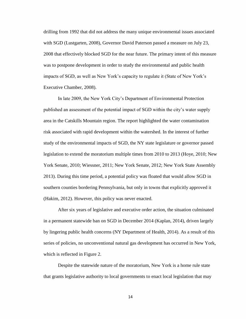
After six years of legislative and executive order action, the situation culminated
in a permanent statewide ban on SGD in December 2014 (Kaplan, 2014), driven largely
by lingering public health concerns (NY Department of Health, 2014). As a result of this
series of policies, no unconventional natural gas development has occurred in New York,
which is reflected in Figure 2.
Despite the statewide nature of the moratorium, New York is a home rule state
that grants legislative authority to local governments to enact local legislation that may
15
limit state-level intrusion into local matters (Stinson, 1997). Given this history and the
discontent with the moratorium, 45 New York towns passed resolutions in support of
SGD in the spring and summer of 2012 (FracTracker, 2014). Fourteen of these towns are
in our sample counties and are shown in Appendix Figure A3. These resolutions were
passed by town councils and were not voted on by residents, but likely reflect residents’
sentiments. The resolutions had no impact on the ability for gas companies to operate in
New York, but were intended to apply political pressure to state policy makers and signal
to industry that these towns are supportive of SGD. One of the major landowner groups
driving the passage of the resolutions, the Joint Landowners Coalition of New York, sued
Governor Cuomo in order to expedite the state’s environmental and public health review
of SGD (De Avila, 2014).
On the other side of the debate, 176 New York towns implemented local bans or
moratoriums on hydraulic fracturing in the event that the statewide moratorium was lifted
(FracTracker, 2014). Most of these townships were located in areas of the state that were
unlikely to experience significant SGD from the Marcellus Shale due to geological
limitations (e.g., low thickness). In our three NY counties, there were only two towns –
Owego (Tioga County) and Wayne (Steuben County) – that passed moratoria on shale
gas development, both in 2012.
3. CONCEPTUAL FRAMEWORK
In this section we present a hedonic property model that incorporates the
phenomena of interest, the valuation of expected shale gas development through the
enactment of a moratorium. The hedonic valuation methodology, originally presented by
16
Rosen (1974), posits that the price of a heterogeneous good can be decomposed into
implicit prices associated with its individual characteristics. By separating the price of the
good into its implicit prices, the technique can help illuminate the value of each
characteristic. The standard hedonic model assumes that all negative and positive
discounted cash flows will be capitalized into the transaction price if there is full
information about those attributes that derive benefits and costs.
We apply the hedonic valuation concept to shale gas development through
housing prices. The price function is given as Ph=Ph(L,S,N,Q(D),G(D)) where L is a
vector of lot characteristics, S is a vector of structural characteristics, N is a vector of
neighborhood characteristics, Q is a vector of environmental characteristics, and G are
geological characteristics that allow for possible shale gas development (e.g., land
overlying shale with retrievable gas). Shale gas development is represented by D.
Geological attributes, G(D), derive value from financial amenities such as lease and
royalty payments that gas companies pay to homeowners to gain access to the shale. The
dis-amenities are represented by the effect on environmental characteristics, Q(D). We
assume that development of the shale would also reduce environmental quality.6 A
homebuyer derives utility from these attributes and a composite good Y, and is expressed
as U(Y, L, S, N, Q(D), G(D)). The homebuyer maximizes utility with respect to a budget
constraint and the expected utility gained from these attributes in relation to the
composite good Y.
Prior to development, the expected flow of benefits and costs coming from shale
6 This also represents other dis-amenities that are not environmental in nature but are costs of shale gas
development that are born through damage caused by noise pollution, damaged roads, and increased
demands on other public infrastructure. We restrict ourselves to this simplified notation for ease of
discussion.
17
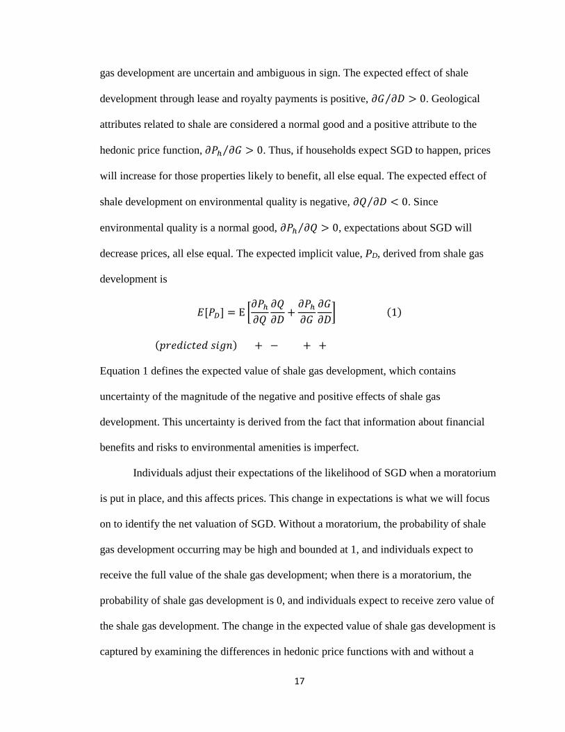
gas development are uncertain and ambiguous in sign. The expected effect of shale
development through lease and royalty payments is positive, 𝜕𝐺 𝜕𝐷⁄ > 0. Geological
attributes related to shale are considered a normal good and a positive attribute to the
hedonic price function, 𝜕𝑃ℎ 𝜕𝐺⁄ > 0. Thus, if households expect SGD to happen, prices
will increase for those properties likely to benefit, all else equal. The expected effect of
shale development on environmental quality is negative, 𝜕𝑄 𝜕𝐷⁄ < 0. Since
environmental quality is a normal good, 𝜕𝑃ℎ 𝜕𝑄⁄ > 0, expectations about SGD will
decrease prices, all else equal. The expected implicit value, PD, derived from shale gas
development is
𝐸[𝑃𝐷] = E [𝜕𝑃ℎ
𝜕𝑄
𝜕𝑄
𝜕𝐷+
𝜕𝑃ℎ
𝜕𝐺
𝜕𝐺
𝜕𝐷] (1)
(𝑝𝑟𝑒𝑑𝑖𝑐𝑡𝑒𝑑 𝑠𝑖𝑔𝑛) + − + +
Equation 1 defines the expected value of shale gas development, which contains
uncertainty of the magnitude of the negative and positive effects of shale gas
development. This uncertainty is derived from the fact that information about financial
benefits and risks to environmental amenities is imperfect.
Individuals adjust their expectations of the likelihood of SGD when a moratorium
is put in place, and this affects prices. This change in expectations is what we will focus
on to identify the net valuation of SGD. Without a moratorium, the probability of shale
gas development occurring may be high and bounded at 1, and individuals expect to
receive the full value of the shale gas development; when there is a moratorium, the
probability of shale gas development is 0, and individuals expect to receive zero value of
the shale gas development. The change in the expected value of shale gas development is
captured by examining the differences in hedonic price functions with and without a
18
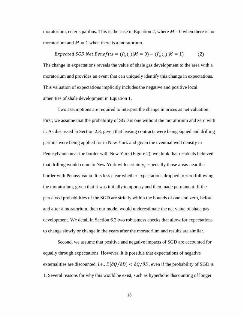
moratorium, ceteris paribus. This is the case in Equation 2, where M = 0 when there is no
moratorium and 𝑀 = 1 when there is a moratorium.
𝐸𝑥𝑝𝑒𝑐𝑡𝑒𝑑 𝑆𝐺𝐷 𝑁𝑒𝑡 𝐵𝑒𝑛𝑒𝑓𝑖𝑡𝑠 = (𝑃ℎ(. )|𝑀 = 0) − (𝑃ℎ(. )|𝑀 = 1) (2)
The change in expectations reveals the value of shale gas development to the area with a
moratorium and provides an event that can uniquely identify this change in expectations.
This valuation of expectations implicitly includes the negative and positive local
amenities of shale development in Equation 1.
Two assumptions are required to interpret the change in prices as net valuation.
First, we assume that the probability of SGD is one without the moratorium and zero with
it. As discussed in Section 2.3, given that leasing contracts were being signed and drilling
permits were being applied for in New York and given the eventual well density in
Pennsylvania near the border with New York (Figure 2), we think that residents believed
that drilling would come to New York with certainty, especially those areas near the
border with Pennsylvania. It is less clear whether expectations dropped to zero following
the moratorium, given that it was initially temporary and then made permanent. If the
perceived probabilities of the SGD are strictly within the bounds of one and zero, before
and after a moratorium, then our model would underestimate the net value of shale gas
development. We detail in Section 6.2 two robustness checks that allow for expectations
to change slowly or change in the years after the moratorium and results are similar.
Second, we assume that positive and negative impacts of SGD are accounted for
equally through expectations. However, it is possible that expectations of negative
externalities are discounted, i.e., 𝐸[𝜕𝑄 𝜕𝐷⁄ ] < 𝜕𝑄 𝜕𝐷⁄ , even if the probability of SGD is
1. Several reasons for why this would be exist, such as hyperbolic discounting of longer
19
term environmental and health impacts, discounting of external consequences of
neighbors’ actions, and uncertainty about well placements. If this assumption does not
hold, our estimate may reflect financial benefits more than costs. Still, this estimate
reveals valuation of expectations about SGD for a population that has not experienced it,
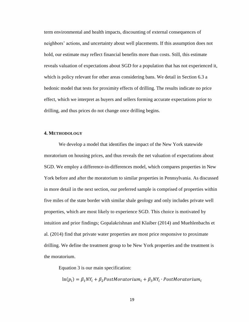
which is policy relevant for other areas considering bans. We detail in Section 6.3 a
hedonic model that tests for proximity effects of drilling. The results indicate no price
effect, which we interpret as buyers and sellers forming accurate expectations prior to
drilling, and thus prices do not change once drilling begins.
4. METHODOLOGY
We develop a model that identifies the impact of the New York statewide
moratorium on housing prices, and thus reveals the net valuation of expectations about
SGD. We employ a difference-in-differences model, which compares properties in New
York before and after the moratorium to similar properties in Pennsylvania. As discussed
in more detail in the next section, our preferred sample is comprised of properties within
five miles of the state border with similar shale geology and only includes private well
properties, which are most likely to experience SGD. This choice is motivated by
intuition and prior findings; Gopalakrishnan and Klaiber (2014) and Muehlenbachs et
al. (2014) find that private water properties are most price responsive to proximate
drilling. We define the treatment group to be New York properties and the treatment is
the moratorium.
Equation 3 is our main specification:
ln(𝑝𝑖) = 𝛽1𝑁𝑌𝑖 + 𝛽2𝑃𝑜𝑠𝑡𝑀𝑜𝑟𝑎𝑡𝑜𝑟𝑖𝑢𝑚𝑖 + 𝛽3𝑁𝑌𝑖 ∙ 𝑃𝑜𝑠𝑡𝑀𝑜𝑟𝑎𝑡𝑜𝑟𝑖𝑢𝑚𝑖
20
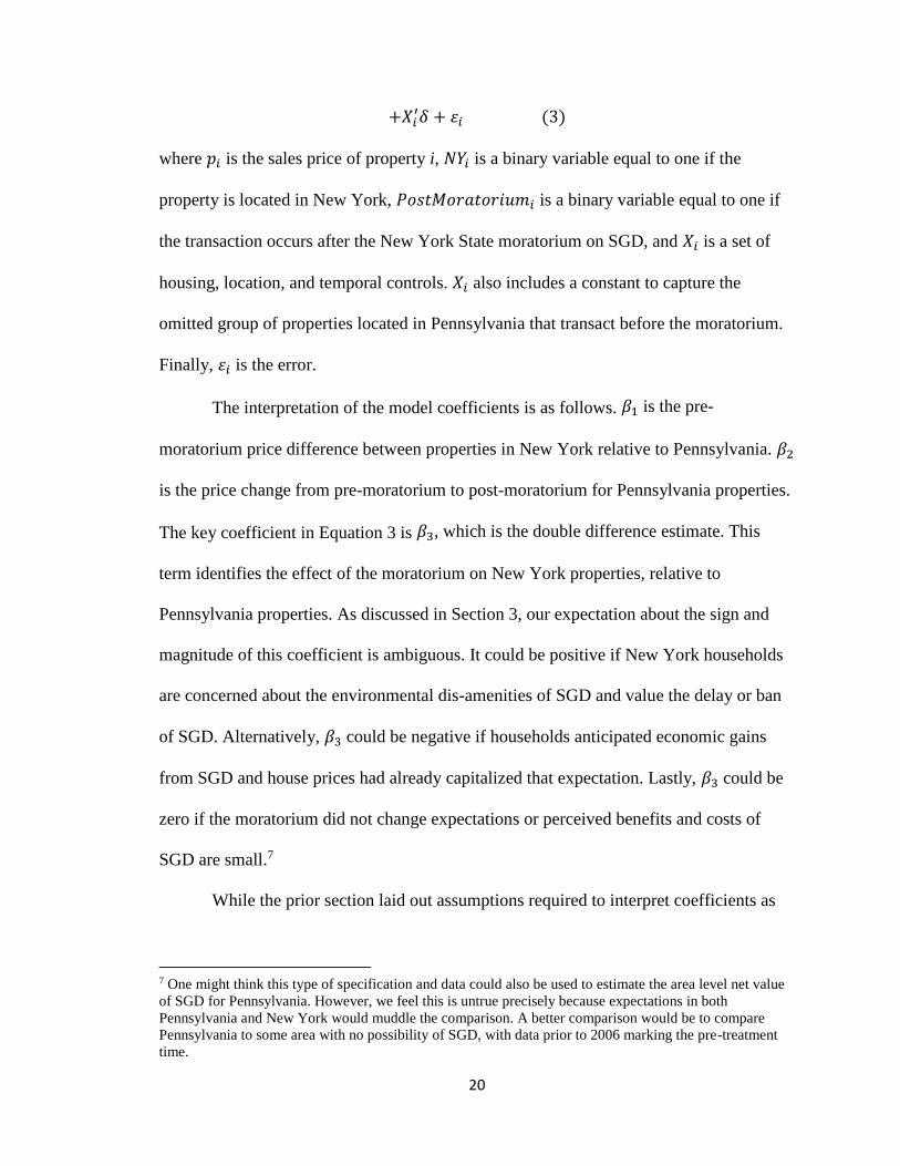
+𝑋𝑖′𝛿 + 휀𝑖 (3)
where 𝑝𝑖 is the sales price of property i, 𝑁𝑌𝑖 is a binary variable equal to one if the
property is located in New York, 𝑃𝑜𝑠𝑡𝑀𝑜𝑟𝑎𝑡𝑜𝑟𝑖𝑢𝑚𝑖 is a binary variable equal to one if
the transaction occurs after the New York State moratorium on SGD, and 𝑋𝑖 is a set of
housing, location, and temporal controls. 𝑋𝑖 also includes a constant to capture the
omitted group of properties located in Pennsylvania that transact before the moratorium.
Finally, 휀𝑖 is the error.
The interpretation of the model coefficients is as follows. 𝛽1 is the pre-
moratorium price difference between properties in New York relative to Pennsylvania. 𝛽2
is the price change from pre-moratorium to post-moratorium for Pennsylvania properties.
The key coefficient in Equation 3 is 𝛽3, which is the double difference estimate. This
term identifies the effect of the moratorium on New York properties, relative to
Pennsylvania properties. As discussed in Section 3, our expectation about the sign and
magnitude of this coefficient is ambiguous. It could be positive if New York households
are concerned about the environmental dis-amenities of SGD and value the delay or ban
of SGD. Alternatively, 𝛽3 could be negative if households anticipated economic gains
from SGD and house prices had already capitalized that expectation. Lastly, 𝛽3 could be
zero if the moratorium did not change expectations or perceived benefits and costs of
SGD are small.7
While the prior section laid out assumptions required to interpret coefficients as
7 One might think this type of specification and data could also be used to estimate the area level net value
of SGD for Pennsylvania. However, we feel this is untrue precisely because expectations in both
Pennsylvania and New York would muddle the comparison. A better comparison would be to compare
Pennsylvania to some area with no possibility of SGD, with data prior to 2006 marking the pre-treatment
time.
21
net valuation, there are also assumptions required for the difference-in-differences design
to be valid. First, we assume that Pennsylvania serves as a good counterfactual for New
York, in terms of house price dynamics. One potential concern is that areas in our study
had different reactions to the US housing market collapse, which is correlated with the
timing of the moratorium. In the Section 5, we show that our sample of Pennsylvania and
New York homes follow a similar price trend pre-moratorium. Also, by focusing on
observations close to the border, we hope to mitigate unobservable determinants of price
trends.8
Our sample choice of five border counties was meant to improve the treatment-
control comparison. Our refinement to focus in particular on properties within 5 miles of
the border with similar shale thickness furthers the strength of the good counterfactual
assumption. However, using bordering counties implicitly assumes that spillover effects
are minimal. Spillover effects could be either environmental or economic. Environmental
spillovers would occur if water or air pollution from SGD were to travel into New York
from Pennsylvania. Evidence from Gopalakrishnan and Klaiber (2014) and
Muehlenbachs et al. (2014) suggests that effects of water pollution are localized at about
2km. SGD in our study area is limited to the Susquehanna River Basin, which flows
south. Thus, any surface water contamination is also likely to flow south further into
Pennsylvania rather than north into New York.9 Economic spillovers are increases in
8 Kuminoff and Pope (2013) find that lower value properties experienced larger boom-bust swings than
higher value properties. Given the differences in price levels between the two states (see Table 1 and Figure
4), it is possible that our Pennsylvania sample experience a larger bust. However, if this was the case, our
estimates would be upward biased, suggesting the impact of the moratorium to be even more negative for
New York prices. To test whether differential boom-bust trends may be impacting our results, we estimate
models that include a series of $100,000 sale price bin fixed effects interacted with year fixed effects to
allow differential boom-bust evolution by price tier. Results are consistent with our main results. 9 An additional possibility is that property owners in pre-moratorium Pennsylvania formed expectations
about environmental spillovers from New York into Pennsylvania in the event of SGD in New York. If
22
employment and spending across the border that indirectly or directly affect the housing
market. Our estimates are unlikely to be affected by any economic spillover because our
sample is restricted to a small area of just five miles on either side of the border, and thus
can be thought of as a single labor market.10 An additional argument that applies to these
two types of spillovers is that New York residents and potential buyers would have
formed expectations about drilling in Pennsylvania and those expectations would be
capitalized into prices prior to the moratorium. Thus, while spillovers may occur, they
should be expected and already accounted for in house prices.
Second, we assume that the treatment (moratorium) had no effect on the control
(Pennsylvania). The main concern here is whether the moratorium on drilling in New
York increased drilling in Pennsylvania. We argue that the pace of development in
Pennsylvania (and elsewhere) was so rapid in the 2008-2011 timeframe that the lack of
drilling in New York had no effect on prices or scarcity in Pennsylvania. Another way for
drilling to be impacted would be if horizontal drills could cross state boundaries and
extract New York gas from Pennsylvania, but this is in fact illegal.11
Third, we assume that the implementation of the New York statewide moratorium
was exogenous to the counties in this study. We believe this is a safe assumption for two
true, then the New York moratorium may have increased prices in Pennsylvania. We argue that this effect
would have been minimal given the evidence of highly localized environmental impacts of drilling from
Gopalakrishnan and Klaiber (2014) and Muehlenbachs et al. (2014). 10 We additionally examined cross border migration to see if individuals relocated from New York to
Pennsylvania after the moratorium. The results, presented in Figure A1 of the appendix, suggest no changes
in migration patterns. 11 It is highly unlikely that horizontal well drilling across state lines has occurred along the NY-PA border.
New York has restrictions on how close one can drill to the state boundary (New York State Regulations –
Environmental Conservation Law 553.1; personal correspondence with Thomas Noll, Section Chief of the
Bureau of Oil & Gas Permitting and Management in the NY DEC Division of Mineral Resources). Though
Pennsylvania does not have an analogous law outlining state border proximity issues, Pennsylvania
Department of Environmental Protection officials note that it is unlikely that any horizontal laterals cross
over into New York from Pennsylvania (personal correspondence with David Engle, Operations Manager
in the Oil & Gas Division of the Pennsylvania Department of Environmental Protection).
23
reasons. One, it is a statewide moratorium, not just a moratorium for the three sample
New York counties, and much of the support for the moratorium came from regions in
New York outside of this sample. Two, many of the sample towns were and still are
against the moratorium as evidenced by the fact that 14 of 37 towns in our New York
sample passed resolutions in support of SGD during the spring and summer of 2012,
while only two towns passed a moratorium.
5. DATA
This study was conducted with property transaction data from five counties along
the New York – Pennsylvania border: Chemung, Steuben, and Tioga counties in New
York; Bradford and Tioga counties in Pennsylvania. We specifically chose these five
counties because 1) the two Pennsylvania counties constitute one of the major clusters of
drilling in that state, 2) all five counties are primarily agricultural and rural in character
and thus make for good comparison, and 3) they border each other so that unobservable
determinants of house prices likely follow similar dynamics.
We obtained transactions and property characteristics data from January 1, 2006
through December 31, 2012 from each county’s property assessment office and New
York’s Office of Real Property Tax Services. Sales prices are adjusted to 2011 levels
using the CPI (U.S. Bureau of Labor Statistics, 2014). For each property in our dataset,
we have information on the number of bedrooms, number of bathrooms, finished living
area, acreage, and age of each property in our dataset. Three of the five counties in our
dataset include multiple transactions per property. However, Bradford County (PA) and
Steuben County (NY) could only provide us with information for the most recent
24
transaction for each property.12
In order to identify each property’s water supply, we use data from
Pennsylvania’s Department of Environmental Protection and New York’s Department of
Taxation and Finance, Office of Real Property Tax Services. Pennsylvania’s data
contains public water supply area boundaries, making sold parcel water supply
identification straightforward. However, New York’s data on water supply access is in
parcel centroid format, which represents every parcel in the state by its center point.
Using parcel boundaries provided by county and regional planning departments, we
connected sales data to water supply data using Geographic Information Systems (GIS).
However, a portion of our sold parcels do not overlay a centroid. In order to identify the
water supply for each parcel in our transaction set, we follow Muehlenbachs et al. (2014)
and create buffers of 100 meters around all public water supply parcel centroids. Then,
we assume that all parcels falling outside of these buffers are dependent on well water.
Figure A2 in the Appendix presents all transactions in our five counties by water type.
The figure makes clear several points. First, private water supply properties are almost
exclusively outside of town boundaries. Second, Pennsylvania has a larger share of
private water properties than New York. Further, there are very few public water
properties within five miles of the border, especially in Pennsylvania.
In total, our original dataset includes 26,138 property transactions across all five
counties from 2006 to 2012. We include only single-family residential and mobile homes
12 We examined how this data limitation may affect results by only using the latest sale for all counties and
coefficients were very similar to the main results presented in Section 6. The results are available upon
request.
25
with private water, which leaves us with 8,466 observations.13 We drop all observations
that sold for less than $10,000 or more than $1,000,000 in 2011 CPI adjusted dollars.
Further, we hypothesize that lot size is a key property characteristic for forming
expectations about benefits and costs to SGD. Pennsylvania has larger lot sizes on
average, so we drop observations that fall outside of the 5% and 95% of the lot size
distribution to ensure common support between our Pennsylvania and New York
samples. Lastly, we drop eight Pennsylvania transactions that occur prior to the
moratorium that are located within two miles of a permitted well. We do this such that
all transactions pre-moratorium have expectations about SGD, but no realized impacts.
Our analysis of the moratorium uses sales in the time span 2006-2011. 2006
marks the beginning of exploration and lease signings in Pennsylvania and New York.
At this point, both properties in Pennsylvania and New York will begin to capitalize
expectations about the benefits and costs to hydraulic fracturing, but have yet to
experience it. We use 2011 as a cutoff because local resolutions begin to be passed in
early 2012. With these cuts, we are left with a sample of 4,976 transactions.
While choosing counties along the border goes a long way towards removing
unobservable differences between New York and Pennsylvania observations, we
develop four samples that further restrict observations. First, in the vein of a border
discontinuity design, two samples are created that limit observations to be within 15
miles of the border and then within five miles of the border. These samples are intended
to further minimize possible bias stemming from unobservable, time-varying processes
13 While mobile homes are often excluded in hedonic analyses such as this, we chose to include them
because a substantial proportion is located on lots greater than half an acre. We present robustness checks
in Section 6 removing mobile homes and results are similar.
26
that differentially affect housing prices across the state boundary. Second, we further
restrict the 15- and 5-mile samples to only include properties that have similar shale
geology. Figure 3 shows the thickness of shale deposits, which is a key driver of
extraction potential.14 On average, our Pennsylvania counties have thicker shale
deposits than in New York, with thickness increasing towards the southeast. In order to
ensure that expectations about SGD are similar on either side of the border, we restrict
observation to be in the 100-200 feet range of thickness. Our preferred sample, shown
by the dashed region of Figure 3, satisfies both the 5-mile border restriction and shale
thickness restriction and includes 1,018 observations.
Table 1 presents summary statistics for several variables of interest. The first
column gives the means for all private water observations in our five counties. The
second and third columns give differences in means for New York versus Pennsylvania
for pre-moratorium samples for all counties (Column 2) and the preferred sample of
observations within 5 miles of the border and of similar shale thickness (Column 3). The
purpose of examining these differences is to determine the comparability of New York
and Pennsylvania. Following Imbens and Wooldridge (2009), we divide the difference in
means by the combined standard deviation to test for substantial differences and mark
differences for which this statistic exceeds 0.25 with an asterisk. Table 1 shows there is
strong statistical overlap between the samples, lending credence to the research design.
We note that the only significant difference is in shale thickness between the samples
which is dramatically reduced by using the restricted sample. There is also convergence
of socioeconomic characteristics as we restrict our sample to tracts just along the border
14 Based on a Marcellus Shale thickness map from the Marcellus Center for Outreach and Research at
Pennsylvania State University.
27
in our study counties, as shown in Appendix Table A4.
As discussed in Section 4, the critical assumption for our difference-in-differences
design to be valid is Pennsylvania must a good counterfactual for New York. The most
common way to support this assumption this is to compare pre-treatment price trends,
and now having introduced the data, we can do just that. Figure 4 displays price trends
for 2006 through July 2008 for the preferred sample. Price trends are similar between
New York and Pennsylvania for private water properties, which further bolsters our
confidence that the counterfactual created by the control counties is appropriate. In
contrast, the pre-moratorium price trends for public water properties do not coincide,
which motivated us to not use these properties in our difference-in-differences design.
One reason for the non-parallel trends could be the small number of Pennsylvania
public water properties near the border. We could expand the sample in order to include
more public water properties (and this does indeed improve the alignment of pre-
treatment trends), but that would defeat the purpose of the border discontinuity. In
addition, we tested whether characteristics of transacted properties were different across
states after the moratorium. The results presented in Table A3 of the online appendix
show that most characteristics, most importantly lot size, are not statistically different
across states.
6. RESULTS
6.1 The effect of the statewide moratorium
Table 2 presents the main results of our analysis of the effect New York’s
statewide moratorium on housing prices (Equation 3). We present the double difference
28
coefficients from five models, each with the same specification, but with progressively
more stringent sample criteria. As controls, all models include a variety of property-
specific characteristics, year fixed effects and township fixed effects. Column 1 includes
all transactions in each of our five sample counties. Column 2 restricts transactions to be
within 15 miles of the border, while Column 3 further restricts transactions to be within
the 100-200 foot shale thickness band. Column 4 requires transactions to be within five
miles of the border, while Column 5 further restricts transactions to be within the 100-
200 foot shale thickness band. Column 5 is our preferred specification as differences in
unobservable characteristics will be minimized with the border restriction and
expectations about SGD should be very similar due to the common thickness.
The coefficient on NY*PostMoratorium in Column 1 is -0.101, which indicates
that private well water properties declined in price 10.1% after the moratorium relative to
similar properties in Pennsylvania. Restricting the sample to within 15 miles of the border
increases the magnitude of the coefficient to -0.13, and the coefficient grows again to -
0.151 when restricting for shale thickness. For the 5 mile sample, the coefficient is -
0.209, and adding shale thickness the coefficient is -0.231. The results present a clear
pattern that coefficients increase in magnitude as sample restrictions are imposed. This
pattern indicates that both the border distance restrictions and the shale thickness
restriction are important for minimizing unobservable variation and aligning expectations
across the border.
Our estimates imply that taking away the expectation of SGD reduces property
values and thus indicates a positive valuation of SGD for areas most likely to experience
both the financial benefits and environmental consequences of SGD. Combining our
29
preferred estimate of -0.231 and the average, pre-moratorium, New York house price in
our preferred sample ($110,526 in $2011), the moratorium reduced house values by
$25,531 on average relative to Pennsylvania. In turn, we interpret this number as the net
present value of an expected stream of costs and benefits of SGD. If we annualize this
present value for a 30-year productive well life with 5% interest, this result translates into
an annual net benefit of $1,649. One assumption underlying this interpretation is that the
probability goes from 1 to 0 with the moratorium. Instead, if subjective probabilities were
within the bounds of 1 and 0, then the net value would be larger and equal to $25,531
divided by the change in probability. For example, if the probability of SGD changed
from 0.9 to 0.4, then the estimated net present value of SGD would be $25,531/(0.9-
0.4)=$51,062.15 The second assumption necessary for our interpretation is that
households have accurate expectations about the benefits and costs that will result from
SGD. For instance, if households are accurate in their assessment of financial benefits,
but discount the possibility of adverse health or environmental consequences, then our
estimate may reflect lost benefits more than the net value. However, in Sections 6.2 and
6.3, we present results that bolster our confidence in these two assumptions.
6.2 Robustness checks and extensions
Table 3 provides a series of robustness checks that probe several key assumptions
15 Another way in which expectations can affect the calculation of net values is if households have a
perceived duration of the moratorium. For example, many people (authors included) had the impression
that the initial moratorium would last five years, and then the New York State government would make a
decision. In this case, the house price reduction is not the lost value of SGD, but the cost of waiting five
years for SGD. At a 5% interest rate, the annualized value of SGD would be $7,618. Given results in
Section 6.2 that households do not seem to be updating their beliefs, we think the assumption that people
believed the moratorium to be temporary is inconsistent with the data. However, future work could
examine more recent data to determine if the permanent ban in 2014 led to any price change.
30
of our difference-in-differences model and our interpretation of the results as revealing
net value of SGD.16 Each column builds on our main result of Column 5 Table 2, and
thus uses both the 5 mile border and shale thickness restrictions. Columns 1 and 2 address
the assumption of expectations changing from 1 to 0 with the moratorium. Column 1
excludes transactions occurring in 2008. As there may have been a gradual slide from
certainty of SGD to uncertainty to certainty of no SGD, removing the time period which
this slide was likely to occur ensures a large discrete and complete change in
expectations. The estimated coefficient is -0.244, which is nearly identical to the main
result. Column 2 includes transactions from 2012, which were originally excluded
because of the local resolution activity that occurred in New York in the spring and
summer of 2012. The coefficient again stays consistent at -0.255, which suggests that
expectations changed with the moratorium and did not change much after that with the
multiple extensions.
Columns 3 and 4 return to the 2006-2011 timespan and test whether alternative
shale geology characteristics may better match expectations across the border. Column 3
restricts the data set to only include those transactions that overlay shale that is 150 to
200 feet thick. The resulting parameter estimate -0.260 is similar to our Table 2 estimate.
Column 4 additionally requires transactions to overlay shale with similar depth.17 Low
depth areas of the shale have relatively lower reservoir pressure and higher water content,
which may reduce potential oil and gas recovery. However, high depth areas of the shale
16 In the appendix, we present additional robustness checks. Table A5 shows the set of control variables.
Table A7 estimates models similar to Table 2, but using the level of prices and results are similar. Table A8
tests for robustness of only including single family homes and using propensity score matching to trim the
sample for covariate balance, and results are similar. Table A9 tests supports the robustness of our 15 mile
border and shale thickness model estimate using models similar to those used in Table 3. 17 Depth is measured based on a Marcellus Shale depth map from the Marcellus Center for Outreach and
Research at Pennsylvania State University.
31
may be less permeable and have higher drilling costs than low depth areas (Advanced
Resources International, 2013). Though ambiguous, it could have an impact on
expectations. The estimate from Column 4 is -0.240, very similar to our estimate without
this additional requirement.
Our research design also assumes that environmental spillovers across the border
are minimal. In Column 5, we remove observations within 1 mile of the border in hope
that any expected or actual spillover is contained to that distance. The estimated
coefficient is -0.231, identical to the main result.18
Our final robustness check, Column 6 in Table 3, further probes how well
Pennsylvania serves as a counterfactual in terms of house price trends. Here, we use a
triple difference specification and include properties that are served by municipal water
supply. These properties are in towns and are unlikely to receive either the financial
benefits or the main environmental damages associated with water contamination. Their
purpose is to serve as an additional control for differential market trends in New York
and Pennsylvania. However, our border discontinuity with a five mile distance
requirement is designed to mitigate these types of unobservable variables. In addition, the
pre-treatment trends did not run parallel (Figure 4), and there are very few public water
properties on the Pennsylvania side (Appendix Figure A4). Thus, we do not believe this
is the best research design, but investigate it as a robustness check. The triple difference
term NY*PostMoratorium*Private, which is now the coefficient of interest, is interpreted
as the change in price due to the moratorium for New York private water supply
18 If instead of a 1 mile exposure buffer of environmental effects, there is a 5 or more mile exposure buffer,
all New York properties in our preferred sample would be exposed. Under this (extreme) assumption, our
estimates would recover the option value of mineral rights.
32
properties, relative to Pennsylvania private water properties, and relative to the
differential change between public water properties in New York and Pennsylvania. The
coefficient estimate is -0.179, which is smaller than the main result and less statistically
significant. While this result is broadly consistent with the main result, the reduced
magnitude is consistent with a pre-moratorium downward trajectory of municipal water
properties in New York relative to Pennsylvania. In sum, the range of estimates from
Table 3 support our assumptions and suggest that the moratorium reduced property
values between 18% and 26% for New York properties overlaying high-quality shale
deposits.
In Table 4, we extend our analysis of the effect of the statewide moratorium by
examining whether there were heterogeneous price impacts based on lot size and future
resolution status of a property’s township.19 Instead of using our preferred 5 mile distance
band in this analysis, we apply a border distance band of 15 miles in order to include
more towns that ultimately passed resolutions in 2012. Larger lots may be able to capture
more financial benefits through leases and royalties. Owners and potential buyers may
expect these financial benefits and so the price decline post-moratorium will be amplified
for larger properties. The first column in Table 4 presents results from a specification that
builds on our double difference framework by interacting lot size (log acres) with each of
the three double difference variables. Resulting parameter estimates indicate that the
double difference coefficient of interest is similar in magnitude to the results from Table
2, Column 3. The interaction with lot size is negative (as expected), but is statistically
19 We also estimate a model with only properties smaller than 10 acres to control for properties that have
substantial differences in values due to quality and size of the land (due to being used for agriculture). We
find our results do not qualitatively change with this restriction.
33
indistinguishable from zero.20 We interpret these results as indicating that there is no
heterogeneity across lot sizes, which we may be due to the high degree of uncertainty in
financial benefits.
The second column of Table 4 explores whether the future resolution status of a
town affects price impacts. As noted above, the statewide moratorium was unpopular in
certain parts of New York. Towns that eventually pass resolutions likely supported SGD
in the 2006-2008 range. Residents and homebuyers may have had larger expectations
about the financial benefits, and thus may have a larger price decrease post-moratorium.
We estimate a specification that is similar to the preferred specification, but additionally
interacts ResolutionTown (= 1 if a property is located in a town that passes a resolution in
2012) with the double difference variable NY*PostMoratorium. The results indicate that
residential property prices declined -12.8% post-moratorium, similar to the estimate
found in Table 2, Column 3. However, we find that this effect does not change in
resolution towns. Although the parameter estimate on the triple difference term is
negative (-9.8%), it is not statistically significant. This result suggests that the underlying
likelihood of SGD as viewed by homeowners and prospective buyers is no different in
resolution towns versus other towns. However, this modeling approach is focused on
selection and underlying characteristics, not the effect of the resolution itself. In the
appendix, we present an analysis of the property value impacts of passing a resolution.
Our results suggest no effect.
6.3 Proximity analysis
20 We also estimated models with different assumptions about the functional form for lot size and results
were similar.
34
In this section we develop a more traditional model that estimates the effect of
proximity to drilling on house prices. Similar to Gopalakrishnan and Klaiber (2014), we
estimate variations on the following model:
ln(𝑝𝑖) = 𝛽1𝑊𝑒𝑙𝑙𝑠𝑖 + 𝛽2𝑊𝑒𝑙𝑙𝑠𝑖 ∙ 𝑃𝑟𝑖𝑣𝑎𝑡𝑒𝑖 + 𝑋𝑖′𝛿 + 휀𝑖 (4)
where 𝑊𝑒𝑙𝑙𝑠𝑖 is the number of wells within a given distance of a property, 𝑃𝑟𝑖𝑣𝑎𝑡𝑒𝑖 is a
binary variable equal to one if the property depends on well water, and 𝑋𝑖 is a set of
housing, location, and temporal controls. Gopalakrishnan and Klaiber (2014) estimate
several specifications varying distance cutoffs and time windows, and we follow suit.
We implement both a one mile and two mile cutoff for the measure of proximity, and
estimate the impact of new wells six and 12 months prior to transaction, as well as any
time prior to transaction. We interact the binary variable 𝑃𝑟𝑖𝑣𝑎𝑡𝑒𝑖 with 𝑊𝑒𝑙𝑙𝑠𝑖 to allow
for heterogeneous effects of proximity over private versus public water. We use all
observations in our threes counties of Pennsylvania from 2006 to 2012. Identification
comes from comparing houses within a given distance band of a drilled shale well to
houses further away and houses that predated the drilling.
While this model has a traditional interpretation of valuation of proximity, this
model also estimates the accuracy of households’ pre-drilling expectations. Because all
transactions in this analysis occurred after households began signing leases with gas
companies, we claim that expectations of SGD net benefits had already been capitalized
into sales prices. Under this interpretation, a post-drilling change in house prices would
suggest that expectations were incorrect. Specifically, if prices decline post-drilling, as
is the case in prior studies, this would indicate that households’ expectations had either
overvalued the financial benefits or undervalued the environmental costs.
35
The results presented in Table 5 suggest that proximity to wells has no effect on
house prices. Across all six specifications, neither the public nor private well water
coefficients are statistically different from zero. These results are qualitatively robust to
changes in functional form. We interpret this to mean that ex ante expectations
established in the initial expansion of SGD in Pennsylvania were on average accurate ex
post. In turn, these results support our claim that New York households near the border
have accurate expectations about SGD. However, an alternative interpretation is there is
no economically significant benefit or cost of living in proximity to drilling.
7. CONCLUSION
This paper proposes to view hedonic analysis through a different lens by focusing
on the formation, realization, and change of expectations to inform environmental policy.
We provide area-level impacts of the statewide moratorium on SGD for households
living in New York. Under assumptions of rational expectations of benefits and costs of
SGD and the statewide moratorium causing a 100% change in expectations about the
probability of SGD, the results are interpreted as the net valuation of the local impacts
of SGD. If expectations did not change 100%, then the estimates could be seen as a
lower bound of SGD value. With loss of the rational expectations assumption, we are
still recovering the effect of the moratorium on property values, which is driven by
expectations over financial benefits and environmental externalities of SGD, and this is
an important estimate for areas considering bans on hydraulic fracturing. Our preferred
model suggests that the moratorium causes a 23.1% price decline for New York
properties most likely to experience SGD, which indicates a positive and substantial
36
valuation of SGD. Our results measuring proximity effects of drilling in Pennsylvania
suggest no price movement after drilling begins. This finding supports the rational
expectations assumption, in that expectations of SGD are formed prior to drilling and
ex post expectations were accurate in regard to the costs and benefits of SGD.
For our preferred border discontinuity sample, our point estimate translates into
a $25,531 loss in equity per house and an annualized loss of $1, 649 per house. In order
to estimate the total property market impact to these three counties, we performed the
following back-of-the-envelope calculation. The average sales price 2006-2008 for a
private water property in our three study counties in New York was $117,283 (in $2011).
Using our -10.1% estimate derived using all properties, the average house lost $11,846 in
value due to the moratorium. From the 2000 Decennial Census, these three counties have
a total of 99,402 housing units. Based on our transactions data, 30% (or 29,848) of these
are likely to have private water supply. Putting these together, we estimate the total net
loss in value for these three New York counties from the moratorium was $354 million.
37
REFERENCES
Advanced Resources International. 2013. “EIA/ARI World Shale Gas and Shale Oil
Resource Assessment.” Report. Prepared for the U.S. Energy Information
Administration, U.S. Department of Energy.
Begos, Kevin. 2012. “Pennsylvania Zoning Laws for Gas Drilling, Known as Act 13,
Debated in State Supreme Court.” Huffington Post, October 18, 2012.
http://www.huffingtonpost.com/2012/10/18/pennsylvania-gas-drilling-
laws_n_1979334.html
Bishop, Kelly C., and Alvin D. Murphy. 2011. “Estimating the Willingness to Pay to
Avoid Violent Crime: A Dynamic Approach.” American Economic Review, 101 (3):
625-629.
Brasier, Kathryn J., Diane K. McLaughlin, Danielle Rhubart, Richard C. Stedman,
Matthew R. Filteau, and Jeffrey Jacquet. 2013. “Risk Perceptions of Natural Gas
Development in the Marcellus Shale.” Environmental Practice, 15: 108-122.
Carter, Kristin M., John A. Harper, Katherine W. Schmid, and Jaime Kostelnik. 2011.
“Unconventional Natural Gas Resources in Pennsylvania: The Backstory of the
Model Marcellus Shale play.” Environmental Geosciences, 18 (4): 217-257.
Clark, Douglas. 2014. Personal communication.
Collins, Alan and Kofi Nkansah, 2013. “Divided Rights, Expanded Conflict: The Impact
of Split Estates in Natural Gas Production.” 2013 Annual Agricultural and Applied
Economics Association Meeting. Washington, DC. No. 150128.
Cornell University Cooperative Extension. 2015. “Frequently Asked Questions.” Cornell
University Natural Gas Research Center.
De Avila, Joseph. 2014. “Pro-Fracking Group Sues New York Gov. Cuomo.” The Wall
Street Journal, February 14, 2014.
http://www.wsj.com/articles/SB10001424052702304315004579383251980462952
Drohan, Patrick J., James C. Finley, Paul Roth, Thomas M. Schuler, Susan L. Stout,
Margaret C. Brittingham, and Nels C. Johnson. 2012. “Oil and Gas Impacts on Forest
Ecosystems: Findings Gleaned from the 2012 Goddard Forum at Penn State
University.” Environmental Practice, 14 (4): 394-399.
Eichler, Alexander. 2013. “Pennsylvania Fracking: A History of Shale Gas Drilling, as
Told by the People Who Live There.” The Huffington Post, January 25, 2013.
38
http://www.huggintonpost.com/2013/01/25/pennsylvania-fracking_n_2440227.html
Energy Information Administration, 2013. “Annual Energy Outlook 2013.” Report. U.S.
Department of Energy.
Evans, Jeffrey S., and Joseph M. Kiesecker. 2014. “Shale Gas, Wind and Water:
Assessing the Potential Cumulative Impacts of Energy Development on Ecosystem
Services within the Marcellus play.” PLoS ONE, 9 (2): e89210.
FracTracker. 2014. High Volume Hydrofracking Bans, Moratoria, and Movements for
Prohibitions in New York State. October 9, 2014.
http://www.fractracker.org/map/us/new-york/moratoria/
Frohlich, Cliff. 2012. “Two-Year Survey Comparing Earthquake Activity and Injection-
Well Locations in the Barnett Shale, Texas.” Proceedings of the National Academy of
Sciences, 109 (35): 13934-13938.
Gopalakrishnan, Sathya, and H. Allen Klaiber. 2013. “Is the Shale Energy Boom a Bust
for Nearby Residents? Evidence from Housing Values in Pennsylvania.” American
Journal of Agricultural Economics, 96 (1): 43-66.
Green, Elwin. 2010. “Marcellus Shale Could Be a Boon or Bane for Landowners.”
Pittsburgh Post-Gazette, February 28, 2010. http://www.post-
gazette.com/business/businessnews/2010/02/28/Marcellus-shale-could-be-a-boon-or-
bane-for-land-owners/stories/201002280253
Grout, Cyrus A., William K. Jaeger, and Andrew J. Plantinga. 2011. “Land-Use
Regulations and Property Values in Portland, Oregon: A Regression Discontinuity
Design Approach.” Regional Science and Urban Economics, 41 (2): 98-107.
Guignet, Dennis. 2013. “What Do Property Values Really Tell Us? A Hedonic Study of
Underground Storage Tanks.” Land Economics, 89 (2): 211–26.
Hakim, Danny. 2012. “Cuomo Proposal Would Restrict Gas Drilling to a Struggling
Area.” The New York Times, June 13, 2012.
http://www.nytimes.com/2012/06/14/nyregion/hydrofracking-under-cuomo-plan-
would-be-restricted-to-a-few-counties.html
Hefley, W. E., et al. 2011. “The Economic Impact of the Value Chain of a Marcellus
Shale Well.” Working Paper, Katz Graduate School of Business. University of
39
Pittsburgh. Pittsburgh, PA.
Hill, Elaine. 2012. “Unconventional Natural Gas Development and Infant Health:
Evidence from Pennsylvania.” Cornell University working paper.
Holmes, Thomas J. (1998), "The Effect of State Policies on the Location of
Manufacturing: Evidence from State Borders," Journal of Political Economy, 106 (4),
667-705.
Hoye, Sarah, 2010. “New York Governor Pauses ‘Fracking’.” CNN, December 13, 2010.
http://www.cnn.com/2010/US/12/13/new.york.fracking.moratorium/
Humphries, Marc. 2008. Memorandum to House Committee on Natural Resources.
Attention: 2008. Congressional Research Service.
Imbens, Guido W., and Jeffrey M. Wooldridge. 2009. “Recent Developments in the
Econometrics of Program Evaluation.” Journal of Economic Literature, 47 (1): 5-86.
Jackson, Robert B., Avner Vengosh, Thomas H. Darrah, Nathaniel R. Warner, Adrian
Down, Robert J. Poreda, Stephen G. Osborn, Kaiguang Zhao, and Jonathan D. Karr.
2013. “Increased Stray Gas Abundance in a Subset of Drinking Water Wells near
Marcellus Shale Gas Extraction.” Proceedings of the National Academy of Sciences,
110(28): 11250-11255.
Kaplan, Thomas. 2014. “Citing Health Risks, Cuomo Bans Fracking in New York State.”
New York Times, December 18, 2014.
http://www.nytimes.com/2014/12/18/nyregion/cuomo-to-ban-fracking-in-new-york-
state-citing-health-risks.html
Kargbo, David M., Ron G. Wilhelm, and David J. Campbell. 2010. “Natural Gas Plays in
the Marcellus Shale: Challenges and Potential Opportunities.” Environmental Science
& Technology, 44: 5679-5684.
Kelsey, Timothy W., Alex Metcalf, and Rodrigo Salcedo. 2012. “Marcellus Shale:
Land Ownership, Local Voice, and the Distribution of Lease and Royalty
Payments.” Report. Center of Economic & Community Development (CECD).
Pennsylvania State University.
Kiviat, Erik. 2013. “Risks to Biodiversity from Hydraulic Fracturing for Natural Gas in
the Marcellus and Utica shales.” Annals of the New York Academy of Sciences,
1286: 1-14.
40
Kulander, Christopher. 2013. “Shale Oil and Gas State Regulatory Issues and Trends.”
Case Western Reserve Law Review, 63 (4): 1101.
Kuminoff, Nicolai V., and Jaren C. Pope. “The Value of Residential Land and Structures
during the Great Housing Boom and Bust.” Land Economics 89, no. 1 (February 1,
2013): 1–29.
Leahy, Andy. 2011. “So When Did New York State’s Moratorium Actually Begin?”
NY Shale Gas Now Blog, November 13, 2010.
http://nyshalegasnow.blogspot.com/2011/11/so-when-did-new-york-states-
marcellus.html
Litovitz, Avisa, Aimee Curtright, Shmuel Abramzon, Nicholas Burger, and Constantine
Samaras. 2013. “Estimation of Regional Air-Quality Damages from Marcellus
Shale Natural Gas Extraction in Pennsylvania.” Environmental Research Letters, 8
(1): 1-8.
Loewenstein, James. 2012. “Natural Gas Royalties in Bradford County Reach $160
Million.” The Daily Review, September 25, 2012.
http://thedailyreview.com/news/natural-gas-royalties-in-bradford-county-reach-160-
million-1.1378260
Lustgarten, Abrahm. 2008. “Governor Signs Drilling Bill but Orders Environmental
Update.” ProPublica, July 23, 2008. http://www.propublica.org/article/governor-
signs-drilling-bill-but-orders-environmental-update-723
Lutz, Brian D., Aurana N. Lewis, and Martin W. Doyle. 2013. “Generation, Transport,
and Disposal of Wastewater Associated with Marcellus Shale Gas Development.”
Water Resources Research, 49: 1-10.
Ma, Lala. 2013. “Learning in a Hedonic Framework: Valuing Brownfield Remediation.”
Working Paper. Duke University.
Mathias, Christopher. 2015. “New York Towns Threaten Secession Over Gov. Cuomo’s
Ban On Fracking.” The Huffington Post, February 20, 2015.
http://www.huffingtonpost.com/2015/02/20/new-york-fracking-secession-southern-
tier-cuomo_n_6722296.html
McKenzie, Lisa M., Roxana Z. Witter, Lee S. Newman, and John L. Adgate. 2012.
“Human Health Risk Assessment of Air Emissions from Development of
41
Unconventional Natural Gas Resources.” Science of The Total Environment, 424: 79-
87.
Messersmith, Dave. 2010. “Natural Gas Pipeline Right-Of-Ways: Understanding
Landowner Rights and Options.” Report. Penn State Cooperative Extension.
Muehlenbachs, Lucija, Elisheba Spiller, and Christopher Timmins. 2014. “The Housing
Market Impacts of Shale Gas Development.” NBER Working Paper No. 19796.
Natural Gas Forum For Landowners. 2014. New York Leasing Forums:
http://www.naturalgasforums.com/smf/index.php/board,20.0.html
Olmstead, Sheila M., Lucija A. Muehlenbachs, Jhih-Shyang Shih, Ziyan Chu, and Alan J.
Krupnick. 2013. “Shale Gas Development Impacts on Surface Water Quality in
Pennsylvania.” Proceedings of the National Academy of Sciences, 110(13): 4962-
4967.
Pennsylvania Department of Environmental Protection. 2012. “Landowners and Oil and
Gas Leases in Pennsylvania.” 8000-FS-DEP2834.
Pennsylvania Department of Environmental Protection. 2014. Water Supply
Determination Letters.
Pope, Jaren. 2008. “Buyer Information and the hedonic: The Impact of a Seller
Disclosure on the Implicit Price for Airport Noise.” Journal of Urban Economics, 63
(2): 498-516.
Powelson, Robert F. 2013. “Annual Report of the Collection and Distribution of Funds
under Act 13 of 2012.” Pennsylvania Public Utility Commission Report.
Rabe, Barry G., and Rachel Hampton. “Taxing Fracking: The Politics of State Severance
Taxes in the Shale Era.” University of Michigan. Center for Local, State, and Urban
Policy Working Paper Series 34
Rahm, Brian G., Josephine T. Bates, Lara R. Pertoia, Amy E. Galford, David A.
Yoxtheimer, and Susan J. Riha. 2013. “Wastewater Management and Marcellus Shale
Gas Development: Trends, Drivers, and Planning Implications.” Journal of
Environmental Management, 120: 105-113.
Rich, Alisa, James P. Grover, and Melanie L. Sattler. 2014. “An Exploratory Study of Air
Emissions Associated with Shale Gas Development and Production in the Barnett
42
Shale.” Journal of the Air & Waste Management Association, 64 (1): 61-72.
Richardson, Nathan, Madeline Gottlieb, Alan Krupnick, and Hannah Wiseman. 2013.
“The State of State Shale Gas Regulation.” Report. Resources for the Future.
Rohlin, Shawn, Stuart S. Rosenthal, and Amanda Ross. “Tax Avoidance and Business
Location in a State Border Model.” Journal of Urban Economics 83 (September
2014): 34–49.
Rosen, Sherwin. 1974. “Hedonic Prices and Implicit Markets: Product Differentiation in
Pure Competition.” Journal of Political Economy, 82 (1): 34-55.
State of New York’s Executive Chamber. 2008. “Governor Patterson Signs Bill
Updating Oil and Gas Drilling Law; Pledges Environmental and Public Health
Safeguards.” Retrieved from:
http://www.governor.ny.gov/archive/paterson/press/press_0723084.html
Stinson, Joe. 1997. “The Home Rule Authority of New York Municipalities in the Land
Use Context.” Report. Pace University Law School.
Turner, Matthew A., Andrew Haughwout, and Wilbert van der Klaauw. 2014. “Land Use
Regulation and Welfare.” Econometrica, 82 (4); 1341-1403.
Weidner, Krista. 2013. “A Landowner’s Guide to Leasing Land in Pennsylvania.”
Pennsylvania State University Cooperative Extension.
Wiessner, Dan. 2011. “NY Assembly Extends Fracking Ban for another Year.” Reuters,
June 6, 2011. http://www.reuters.com/article/2011/06/06/us-newyork-fracking-
idUSTRE7556RR20110606
Wilber, Tom. 2014. “How Fracking Got Stopped in New York.” Originally published in
the Binghamton Press & Sun Bulletin, December 22, 2014.
http://tomwilber.blogspot.com/2014/12/how-fracking-got-stopped-in-new-york.html
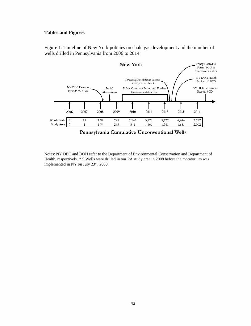
43
Tables and Figures
Figure 1: Timeline of New York policies on shale gas development and the number of
wells drilled in Pennsylvania from 2006 to 2014
Notes: NY DEC and DOH refer to the Department of Environmental Conservation and Department of
Health, respectively. * 5 Wells were drilled in our PA study area in 2008 before the moratorium was
implemented in NY on July 23rd, 2008
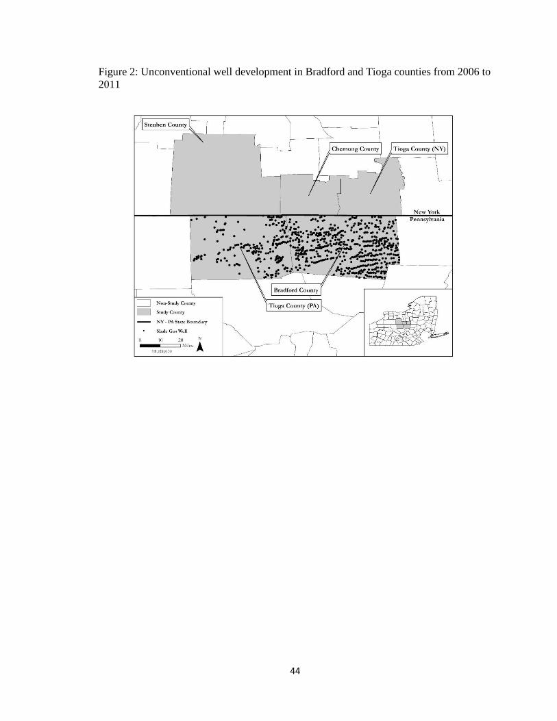
44
Figure 2: Unconventional well development in Bradford and Tioga counties from 2006 to
2011
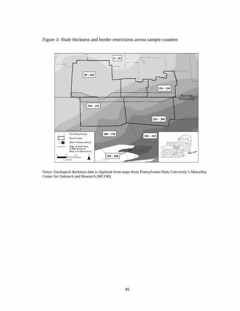
45
Figure 3: Shale thickness and border restrictions across sample counties
Notes: Geological thickness data is digitized from maps from Pennsylvania State University’s Marcellus
Center for Outreach and Research (MCOR).
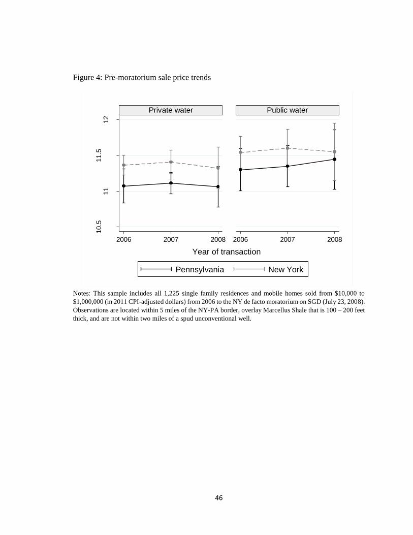
46
Figure 4: Pre-moratorium sale price trends
Notes: This sample includes all 1,225 single family residences and mobile homes sold from $10,000 to
$1,000,000 (in 2011 CPI-adjusted dollars) from 2006 to the NY de facto moratorium on SGD (July 23, 2008).
Observations are located within 5 miles of the NY-PA border, overlay Marcellus Shale that is 100 – 200 feet
thick, and are not within two miles of a spud unconventional well.
10.5
11
11.5
12
2006 2007 2008 2006 2007 2008
Private water Public water
Pennsylvania New York
Lo
g s
ale
s p
rice
Year of transaction
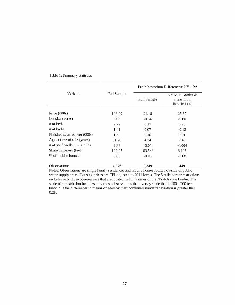
47
Table 1: Summary statistics
Variable Full Sample
Pre-Moratorium Differences: NY - PA
Full Sample
< 5 Mile Border &
Shale Trim
Restrictions
Price (000s) 108.09 24.18 25.67
Lot size (acres) 3.06 -0.54 -0.60
# of beds 2.79 0.17 0.20
# of baths 1.41 0.07 -0.12
Finished squared feet (000s) 1.52 0.10 0.01
Age at time of sale (years) 51.20 4.34 7.40
# of spud wells: 0 - 3 miles 2.33 -0.01 -0.004
Shale thickness (feet) 190.07 -63.54* 8.10*
% of mobile homes 0.08 -0.05 -0.08
Observations 4,976 2,349 449
Notes: Observations are single family residences and mobile homes located outside of public
water supply areas. Housing prices are CPI-adjusted to 2011 levels. The 5 mile border restrictions
includes only those observations that are located within 5 miles of the NY-PA state border. The
shale trim restriction includes only those observations that overlay shale that is 100 - 200 feet
thick. * if the differences in means divided by their combined standard deviation is greater than
0.25.
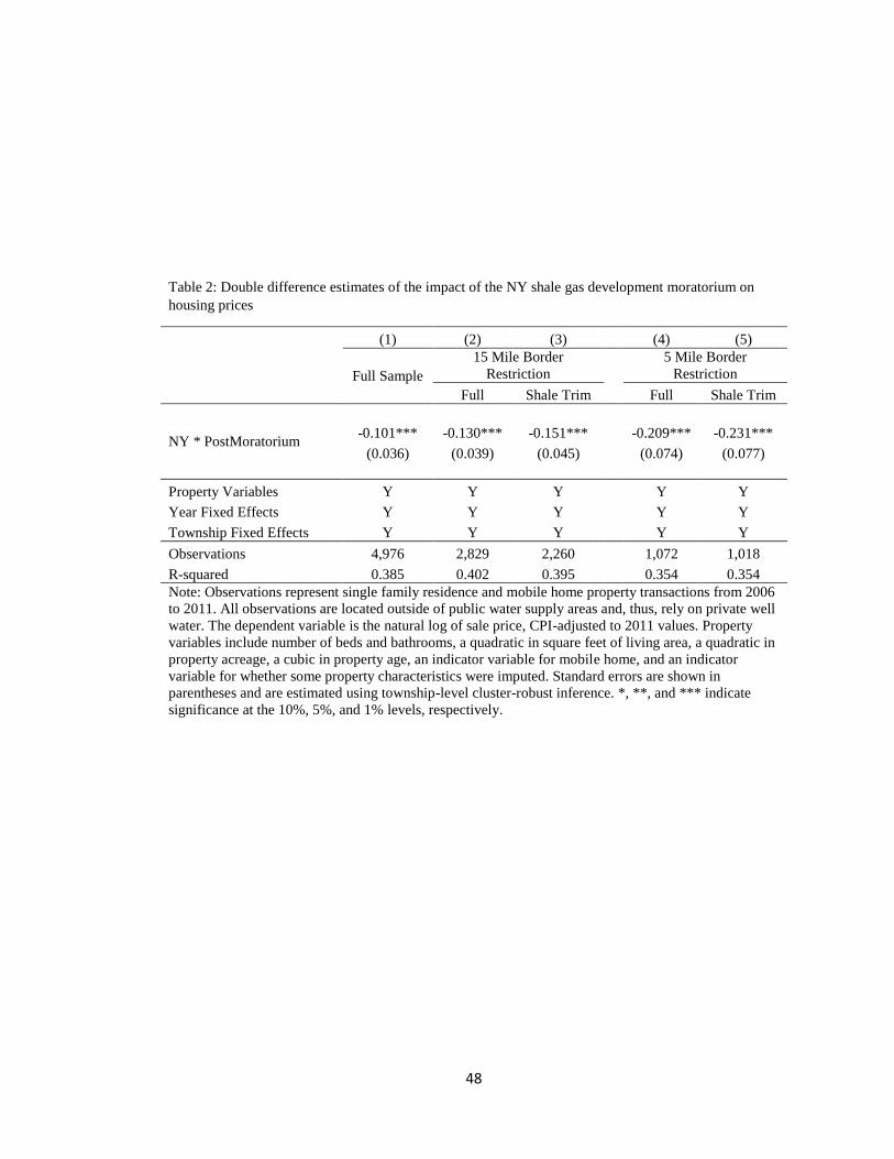
48
Table 2: Double difference estimates of the impact of the NY shale gas development moratorium on
housing prices
(1) (2) (3) (4) (5)
Full Sample
15 Mile Border
Restriction
5 Mile Border
Restriction
Full Shale Trim Full Shale Trim
NY * PostMoratorium -0.101*** -0.130*** -0.151*** -0.209*** -0.231***
(0.036) (0.039) (0.045) (0.074) (0.077)
Property Variables Y Y Y Y Y
Year Fixed Effects Y Y Y Y Y
Township Fixed Effects Y Y Y Y Y
Observations 4,976 2,829 2,260 1,072 1,018
R-squared 0.385 0.402 0.395 0.354 0.354
Note: Observations represent single family residence and mobile home property transactions from 2006
to 2011. All observations are located outside of public water supply areas and, thus, rely on private well
water. The dependent variable is the natural log of sale price, CPI-adjusted to 2011 values. Property
variables include number of beds and bathrooms, a quadratic in square feet of living area, a quadratic in
property acreage, a cubic in property age, an indicator variable for mobile home, and an indicator
variable for whether some property characteristics were imputed. Standard errors are shown in
parentheses and are estimated using township-level cluster-robust inference. *, **, and *** indicate
significance at the 10%, 5%, and 1% levels, respectively.
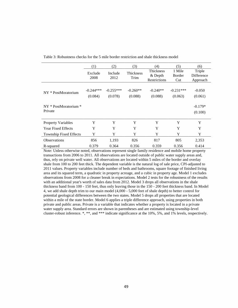
49
Table 3: Robustness checks for the 5 mile border restriction and shale thickness model
(1) (2) (3) (4) (5) (6)
Exclude
2008
Include
2012
Thickness
Trim
Thickness
& Depth
Restrictions
1 Mile
Border
Cut
Triple
Difference
Approach
NY * PostMoratorium -0.244*** -0.255*** -0.260** -0.240** -0.231*** -0.050
(0.084) (0.078) (0.088) (0.088) (0.063) (0.061)
NY * PostMoratorium *
Private
-0.179*
(0.100)
Property Variables Y Y Y Y Y Y
Year Fixed Effects Y Y Y Y Y Y
Township Fixed Effects Y Y Y Y Y Y
Observations 856 1,193 826 817 805 2,353
R-squared 0.379 0.364 0.356 0.359 0.356 0.414
Note: Unless otherwise noted, observations represent single family residence and mobile home property
transactions from 2006 to 2011. All observations are located outside of public water supply areas and,
thus, rely on private well water. All observations are located within 5 miles of the border and overlay
shale from 100 to 200 feet thick. The dependent variable is the natural log of sale price, CPI-adjusted to
2011 values. Property variables include number of beds and bathrooms, square footage of finished living
area and its squared term, a quadratic in property acreage, and a cubic in property age. Model 1 excludes
observations from 2008 for a cleaner break in expectations. Model 2 tests for the robustness of the results
with an additional year's worth of sales data from 2012. Model 3 drops all observations in the shale
thickness band from 100 - 150 feet, thus only leaving those in the 150 - 200 feet thickness band. In Model
4, we add shale depth trim to our main model (4,000 - 5,000 feet of shale depth) to better control for
potential geological differences between the two states. Model 5 drops all properties that are located
within a mile of the state border. Model 6 applies a triple difference approach, using properties in both
private and public areas. Private is a variable that indicates whether a property is located in a private
water supply area. Standard errors are shown in parentheses and are estimated using township-level
cluster-robust inference. *, **, and *** indicate significance at the 10%, 5%, and 1% levels, respectively.
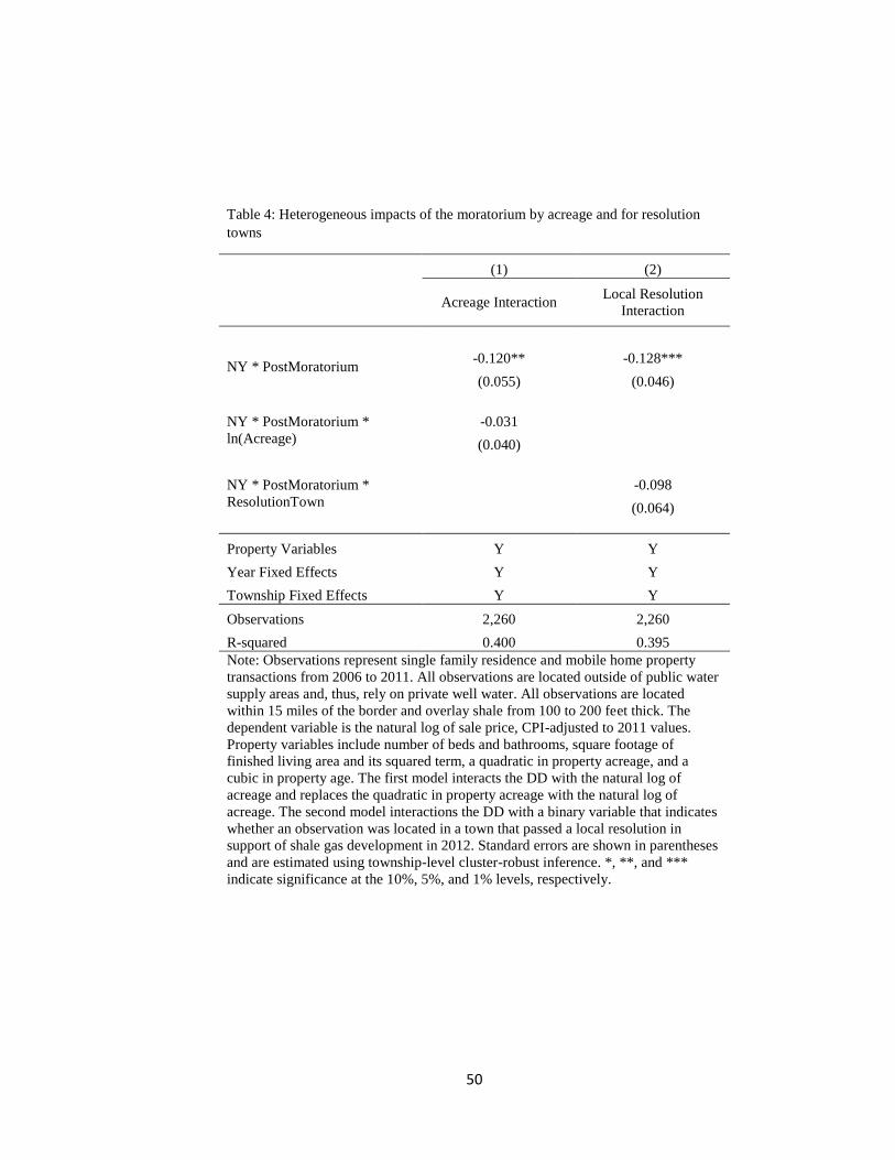
50
Table 4: Heterogeneous impacts of the moratorium by acreage and for resolution
towns
(1) (2)
Acreage Interaction Local Resolution
Interaction
NY * PostMoratorium -0.120** -0.128***
(0.055) (0.046)
NY * PostMoratorium *
ln(Acreage)
-0.031
(0.040)
NY * PostMoratorium *
ResolutionTown
-0.098
(0.064)
Property Variables Y Y
Year Fixed Effects Y Y
Township Fixed Effects Y Y
Observations 2,260 2,260
R-squared 0.400 0.395
Note: Observations represent single family residence and mobile home property
transactions from 2006 to 2011. All observations are located outside of public water
supply areas and, thus, rely on private well water. All observations are located
within 15 miles of the border and overlay shale from 100 to 200 feet thick. The
dependent variable is the natural log of sale price, CPI-adjusted to 2011 values.
Property variables include number of beds and bathrooms, square footage of
finished living area and its squared term, a quadratic in property acreage, and a
cubic in property age. The first model interacts the DD with the natural log of
acreage and replaces the quadratic in property acreage with the natural log of
acreage. The second model interactions the DD with a binary variable that indicates
whether an observation was located in a town that passed a local resolution in
support of shale gas development in 2012. Standard errors are shown in parentheses
and are estimated using township-level cluster-robust inference. *, **, and ***
indicate significance at the 10%, 5%, and 1% levels, respectively.
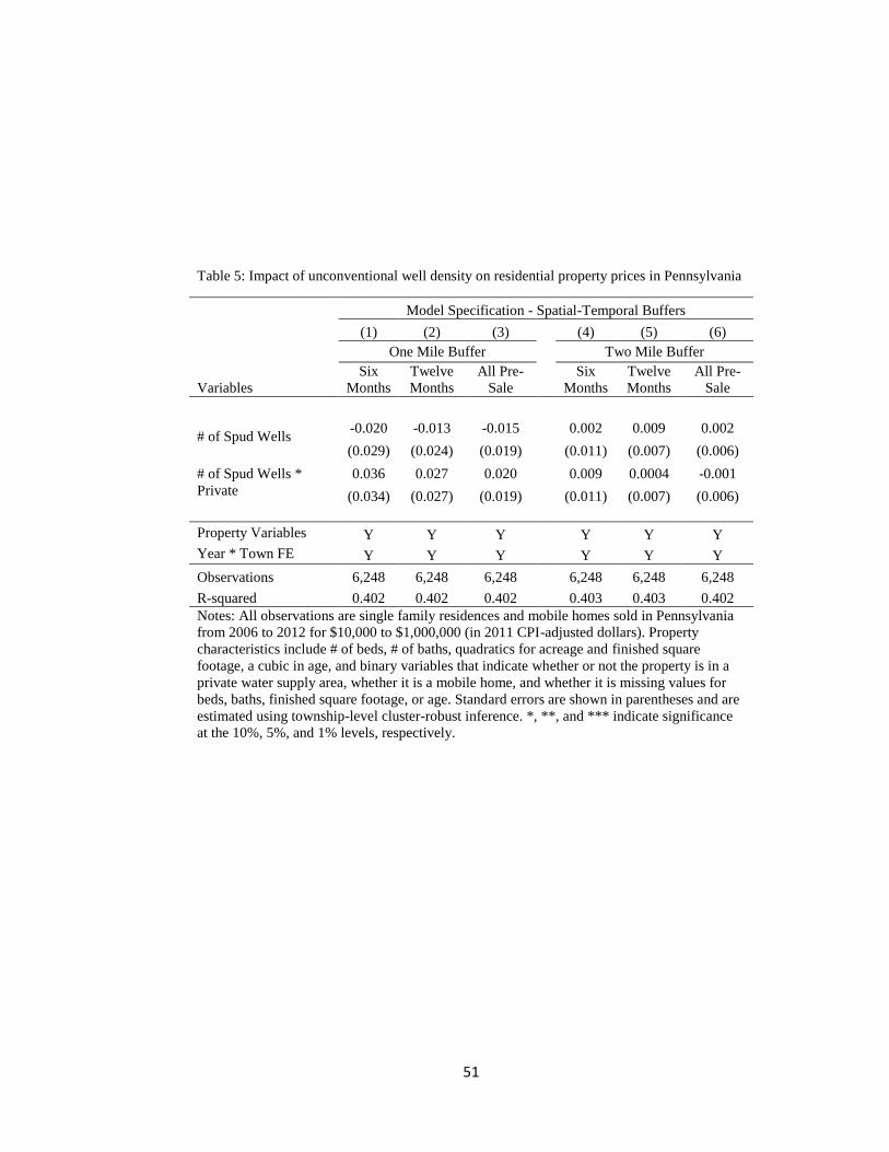
51
Table 5: Impact of unconventional well density on residential property prices in Pennsylvania
Model Specification - Spatial-Temporal Buffers
Variables
(1) (2) (3) (4) (5) (6)
One Mile Buffer Two Mile Buffer
Six
Months
Twelve
Months
All Pre-
Sale
Six
Months
Twelve
Months
All Pre-
Sale
# of Spud Wells -0.020 -0.013 -0.015 0.002 0.009 0.002
(0.029) (0.024) (0.019) (0.011) (0.007) (0.006)
# of Spud Wells *
Private
0.036 0.027 0.020 0.009 0.0004 -0.001
(0.034) (0.027) (0.019) (0.011) (0.007) (0.006)
Property Variables Y Y Y Y Y Y
Year * Town FE Y Y Y Y Y Y
Observations 6,248 6,248 6,248 6,248 6,248 6,248
R-squared 0.402 0.402 0.402 0.403 0.403 0.402
Notes: All observations are single family residences and mobile homes sold in Pennsylvania
from 2006 to 2012 for $10,000 to $1,000,000 (in 2011 CPI-adjusted dollars). Property
characteristics include # of beds, # of baths, quadratics for acreage and finished square
footage, a cubic in age, and binary variables that indicate whether or not the property is in a
private water supply area, whether it is a mobile home, and whether it is missing values for
beds, baths, finished square footage, or age. Standard errors are shown in parentheses and are
estimated using township-level cluster-robust inference. *, **, and *** indicate significance
at the 10%, 5%, and 1% levels, respectively.
52
Appendix
This appendix provides information, data, and results that supplement, but are not
critical to, the analysis in our main paper.
Tables A1 and A2 provide information regarding the monetary benefits and
environmental costs, respectively, which may accrue to landowners in areas with active
shale gas development. These supplement the discussion in Sections 2.1-2.2 of the main
text. Although we focus on environmental costs, other costs from SGD could be social in
nature, such as increased inequality and vulnerability of poor community members
(Schafft et al., 2014), strains on local road infrastructure (Miller and Sassin, 2014), and
community cultural changes (Jacquet and Kay, 2014).
Table A3 gives summary statistics for housing characteristics post-moratorium.
This table is identical in structure to Table 1 from the main text. The purpose of this table
is to test whether characteristics of transacting properties differed after the moratorium. If
the types of properties did change, then this would discredit our main difference-in-
differences estimates. The table shows that transacting New York properties are older
than Pennsylvania properties. The table also shows that shale thickness is greater in the
New York sample, as it is pre-moratorium, and the distance to spud wells is greater in
New York than in Pennsylvania, which is expected. Most importantly, lot size is not
significantly different between the states. Thus, we see no reason to believe that changes
in the types of properties that transact will affect our estimates.
Table A4 highlights differences in means for a variety of census tract-level
variables between New York and Pennsylvania (U.S. Census 2000). The table tests for
53
whether New York and Pennsylvania are significantly different from each other in terms
of demographic, economic, and social characteristics. We break up the states into three
subsets: (i) full state, (ii) study counties, and (iii) all census tracts in our study counties
that are adjacent to the state boundary. By testing for statistical differences across
different subsets of the states, we identify whether these characteristics converge as we
move closer to our primary study area adjacent to the border. Results indicate that there
are significant differences in demographic, economic, and social characteristics between
New York and Pennsylvania at the state level. Although the absolute differences start to
decrease when we restrict the census tract subset to only include those within our five
study counties, we still observe significant differences in racial characteristics, rental
occupancy percentage, and the unemployment rate. Once we restrict our sample to
include only those census tract observations along the state border, we find that the only
statistically-significant difference between the two states is median age. This is an
important result, as it strengthens our argument that by focusing our analysis along the
state border, we improve the comparability between our treatment and control groups.
Table A5 uses our preferred sample from Column 5 of Table 2 (properties within
five miles of the border with shale geology overlap) and tests how functional form
assumptions affect estimates. Results are consistent across specifications.
Table A6 provides our comprehensive model results including parameter
estimates on all covariates included in our models. All estimates have the expected sign.
In Table A7, we estimate Table 2 from the main paper using Linear-Linear
models with the understanding that the value of shale development is likely to be similar
across the spectrum of sale prices. Our model estimates indicate that New York
54
properties that are most likely to experience shale development value it in the range of
$10,000 to $28,000. Given mean sale price values for our subsample, the results are
qualitatively similar whether you use a Log-Linear or Linear-Linear, making the average
effect of the moratorium the same regardless of using logs or levels.
Table A8 provides a series of robustness checks on our results from Table 2,
Column 5 (additional to those found in Table 3), while Table A9 tests the robustness of
our results from Table 2, Column 3 (by estimating a similar series of models from Table
3). Results from both tables provide additional support to those found in the main text.
Figure A1 examines household movement across the border. One threat to our
identification strategy is spillovers across the border caused by the moratorium. Using
IRS migration data from our five sample counties, we compare the number of people
moving from New York to Pennsylvania and vice versa. Figure A1 shows parallel trends
both before and after the moratorium, giving credence to our identification assumptions.
Figure A2 shows the locations of residential property sales in our study area from
2006 to 2011 by water type.
Figure A3 shows the locations of towns in our study area that have passed SGD-
supporting townships, while Figure A4 shows shale depth across our study area with an
outlined 5-mile state border restriction buffer.
Analysis of Property Price Impacts of Local Resolutions in Favor of SGD
In addition to examining the effect of the statewide moratoria, we explore the
effect of town-level resolutions in support of SGD on housing prices. While local
resolutions had no direct effect on actual drilling activity, it is possible that passing a
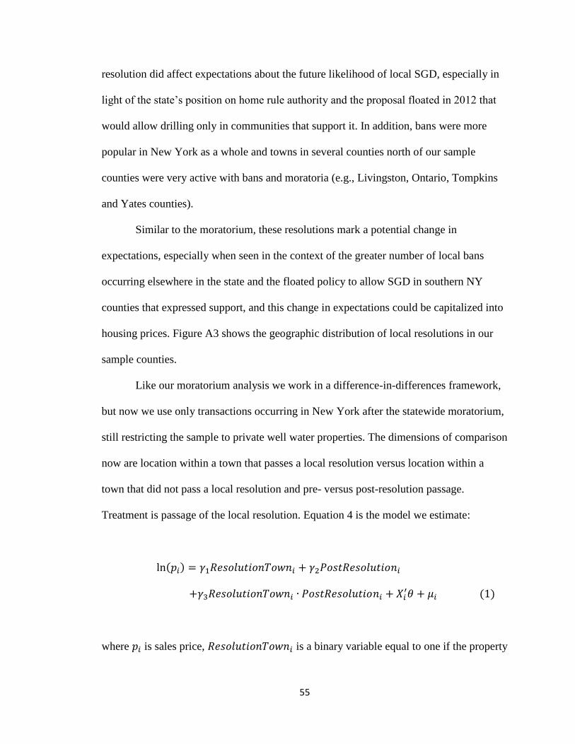
55
resolution did affect expectations about the future likelihood of local SGD, especially in
light of the state’s position on home rule authority and the proposal floated in 2012 that
would allow drilling only in communities that support it. In addition, bans were more
popular in New York as a whole and towns in several counties north of our sample
counties were very active with bans and moratoria (e.g., Livingston, Ontario, Tompkins
and Yates counties).
Similar to the moratorium, these resolutions mark a potential change in
expectations, especially when seen in the context of the greater number of local bans
occurring elsewhere in the state and the floated policy to allow SGD in southern NY
counties that expressed support, and this change in expectations could be capitalized into
housing prices. Figure A3 shows the geographic distribution of local resolutions in our
sample counties.
Like our moratorium analysis we work in a difference-in-differences framework,
but now we use only transactions occurring in New York after the statewide moratorium,
still restricting the sample to private well water properties. The dimensions of comparison
now are location within a town that passes a local resolution versus location within a
town that did not pass a local resolution and pre- versus post-resolution passage.
Treatment is passage of the local resolution. Equation 4 is the model we estimate:
ln(𝑝𝑖) = 𝛾1𝑅𝑒𝑠𝑜𝑙𝑢𝑡𝑖𝑜𝑛𝑇𝑜𝑤𝑛𝑖 + 𝛾2𝑃𝑜𝑠𝑡𝑅𝑒𝑠𝑜𝑙𝑢𝑡𝑖𝑜𝑛𝑖
+𝛾3𝑅𝑒𝑠𝑜𝑙𝑢𝑡𝑖𝑜𝑛𝑇𝑜𝑤𝑛𝑖 ∙ 𝑃𝑜𝑠𝑡𝑅𝑒𝑠𝑜𝑙𝑢𝑡𝑖𝑜𝑛𝑖 + 𝑋𝑖′𝜃 + 𝜇𝑖 (1)
where 𝑝𝑖 is sales price, 𝑅𝑒𝑠𝑜𝑙𝑢𝑡𝑖𝑜𝑛𝑇𝑜𝑤𝑛𝑖 is a binary variable equal to one if the property
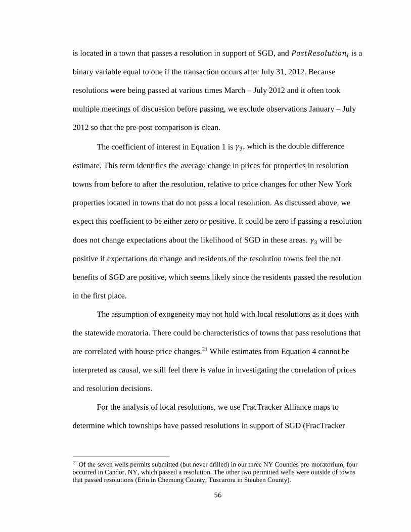
56
is located in a town that passes a resolution in support of SGD, and 𝑃𝑜𝑠𝑡𝑅𝑒𝑠𝑜𝑙𝑢𝑡𝑖𝑜𝑛𝑖 is a
binary variable equal to one if the transaction occurs after July 31, 2012. Because
resolutions were being passed at various times March – July 2012 and it often took
multiple meetings of discussion before passing, we exclude observations January – July
2012 so that the pre-post comparison is clean.
The coefficient of interest in Equation 1 is 𝛾3, which is the double difference
estimate. This term identifies the average change in prices for properties in resolution
towns from before to after the resolution, relative to price changes for other New York
properties located in towns that do not pass a local resolution. As discussed above, we
expect this coefficient to be either zero or positive. It could be zero if passing a resolution
does not change expectations about the likelihood of SGD in these areas. 𝛾3 will be
positive if expectations do change and residents of the resolution towns feel the net
benefits of SGD are positive, which seems likely since the residents passed the resolution
in the first place.
The assumption of exogeneity may not hold with local resolutions as it does with
the statewide moratoria. There could be characteristics of towns that pass resolutions that
are correlated with house price changes.21 While estimates from Equation 4 cannot be
interpreted as causal, we still feel there is value in investigating the correlation of prices
and resolution decisions.
For the analysis of local resolutions, we use FracTracker Alliance maps to
determine which townships have passed resolutions in support of SGD (FracTracker
21 Of the seven wells permits submitted (but never drilled) in our three NY Counties pre-moratorium, four
occurred in Candor, NY, which passed a resolution. The other two permitted wells were outside of towns
that passed resolutions (Erin in Chemung County; Tuscarora in Steuben County).
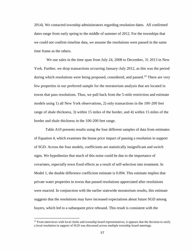
57
2014). We contacted township administrators regarding resolution dates. All confirmed
dates range from early spring to the middle of summer of 2012. For the townships that
we could not confirm timeline data, we assume the resolutions were passed in the same
time frame as the others.
We use sales in the time span from July 24, 2008 to December, 31 2013 in New
York. Further, we drop transactions occurring January-July 2012, as this was the period
during which resolutions were being proposed, considered, and passed.22 There are very
few properties in our preferred sample for the moratorium analysis that are located in
towns that pass resolutions. Thus, we pull back from the 5-mile restriction and estimate
models using 1) all New York observations, 2) only transactions in the 100-200 feet
range of shale thickness, 3) within 15 miles of the border, and 4) within 15 miles of the
border and shale thickness in the 100-200 feet range.
Table A10 presents results using the four different samples of data from estimates
of Equation 4, which examines the house price impact of passing a resolution in support
of SGD. Across the four models, coefficients are statistically insignificant and switch
signs. We hypothesize that much of this noise could be due to the importance of
covariates, especially town fixed effects as a result of self-selection into treatment. In
Model 1, the double difference coefficient estimate is 0.094. This estimate implies that
private water properties in towns that passed resolutions appreciated after resolutions
were enacted. In conjunction with the earlier statewide moratorium results, this estimate
suggests that the resolutions may have increased expectations about future SGD among
buyers, which led to a subsequent price rebound. This result is consistent with the
22 From interviews with local clerks and township board representatives, it appears that the decision to ratify
a local resolution in support of SGD was discussed across multiple township board meetings.
58
moratorium results in that it indicates positive valuation of SGD. Again, as argued in
Section 2.3, these resolutions occurred in the backdrop of the more popular local bans
and moratoria. While the resolutions are meaningless in that they do not affect SGD, they
may influence expectations about what will happen in the town in the event that the
statewide moratorium is eventually lifted.
However, restricted subsets of the data indicate negative double difference
coefficient estimates in the range of -0.074 to -0.183. With the caveat that these
coefficients are not statistically different than zero, the point estimates suggest that
properties located within resolution towns depreciated post-resolution, relative to similar
properties elsewhere. The contradiction in results between Model 1 and Models 2-4 and
large standard errors suggest that the relationship either is ambiguous or cannot be
measured with our sample counties.
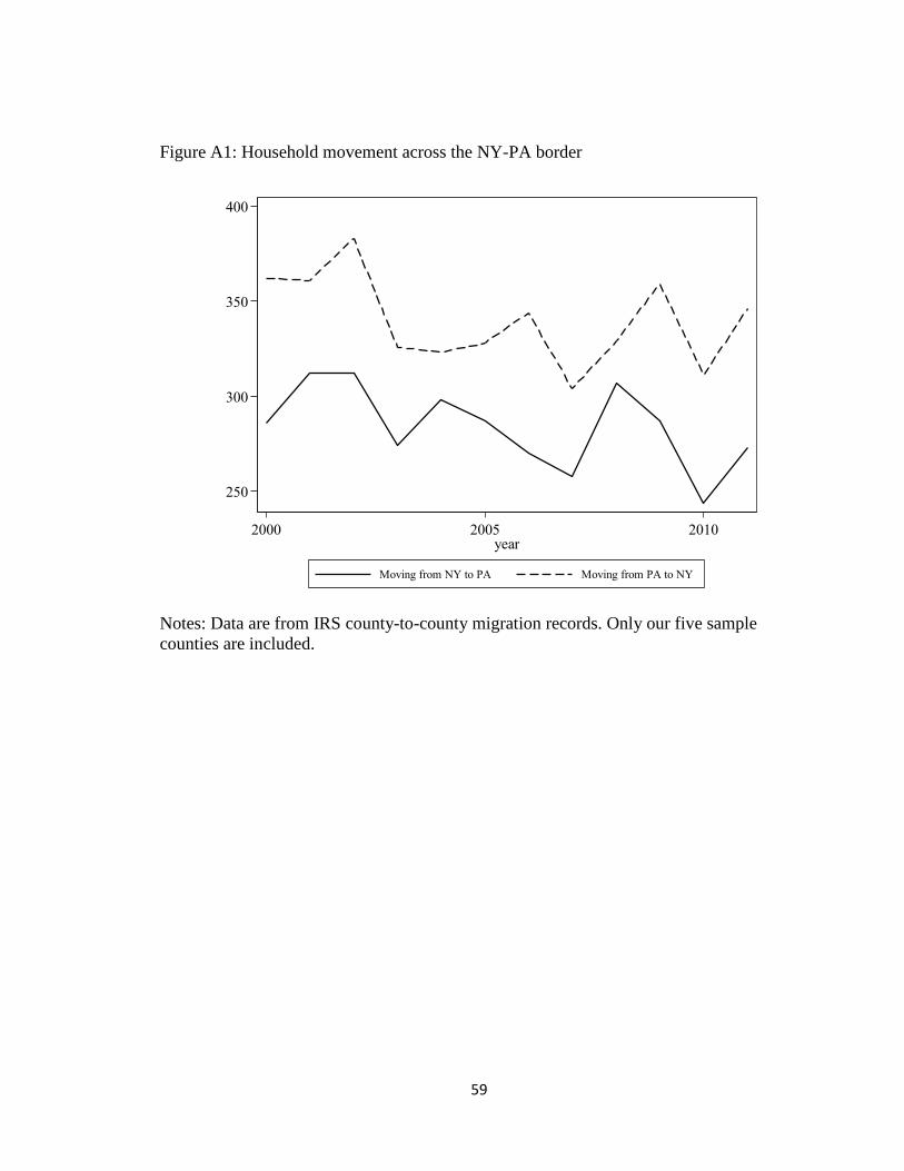
59
Figure A1: Household movement across the NY-PA border
Notes: Data are from IRS county-to-county migration records. Only our five sample
counties are included.
250
300
350
400
Num
ber
of
house
hold
s
2000 2005 2010year
Moving from NY to PA Moving from PA to NY
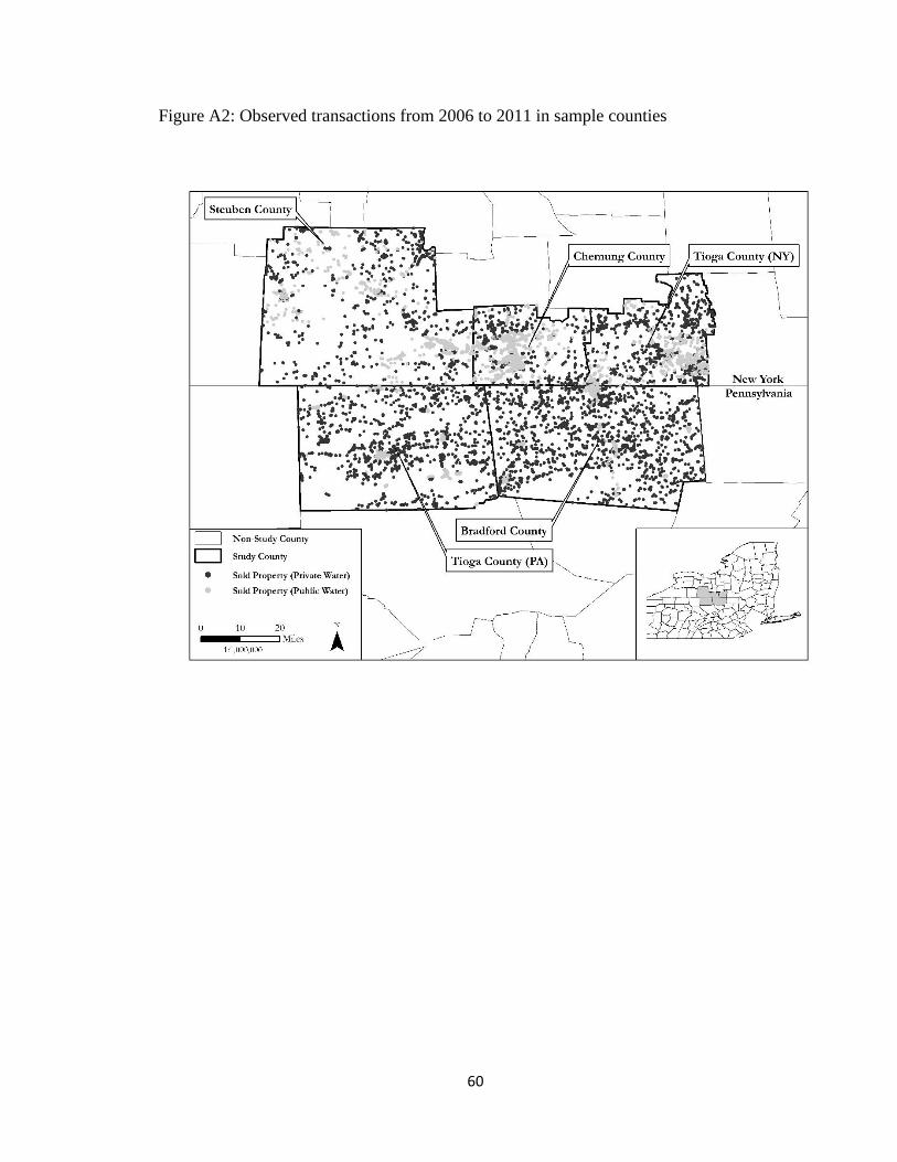
60
Figure A2: Observed transactions from 2006 to 2011 in sample counties
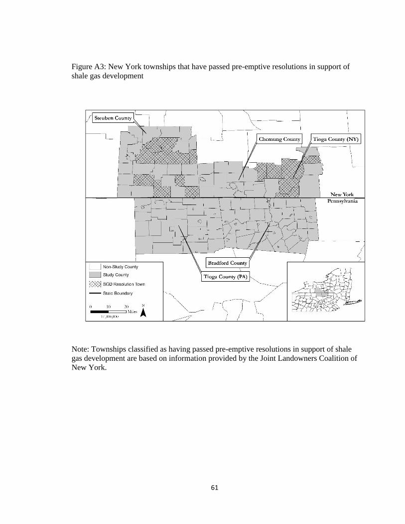
61
Figure A3: New York townships that have passed pre-emptive resolutions in support of
shale gas development
Note: Townships classified as having passed pre-emptive resolutions in support of shale
gas development are based on information provided by the Joint Landowners Coalition of
New York.
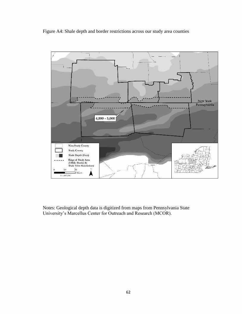
62
Figure A4: Shale depth and border restrictions across our study area counties
Notes: Geological depth data is digitized from maps from Pennsylvania State
University’s Marcellus Center for Outreach and Research (MCOR).
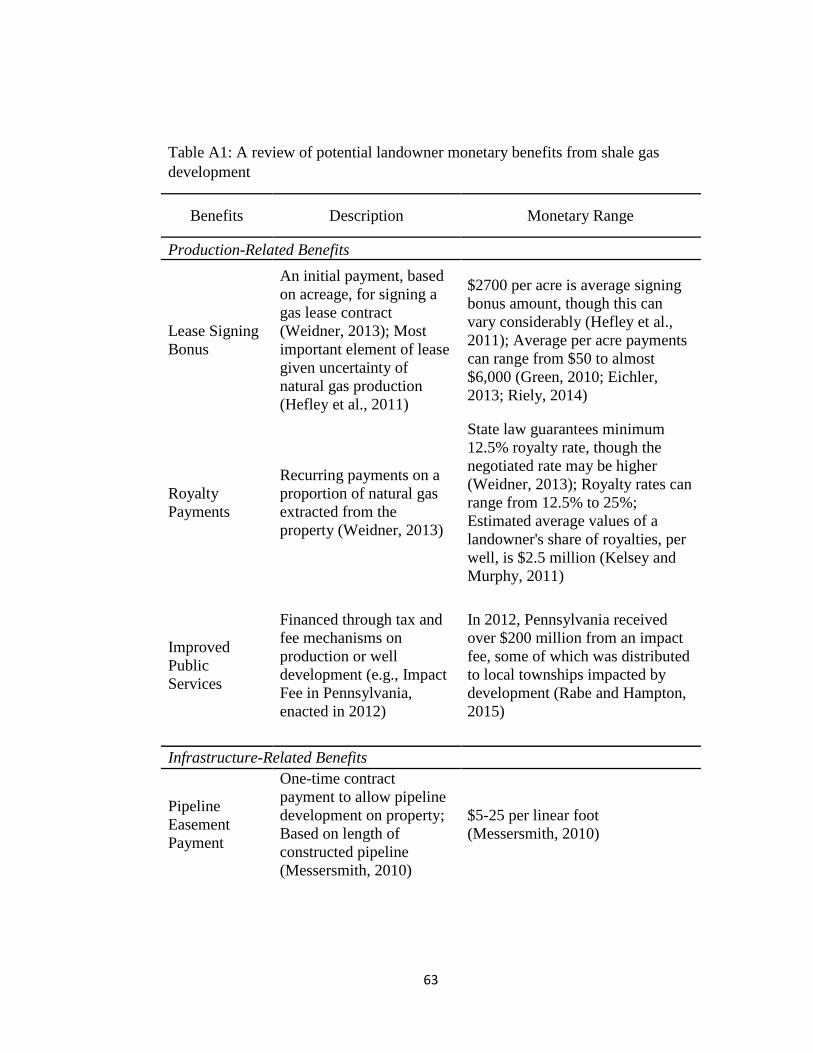
63
Table A1: A review of potential landowner monetary benefits from shale gas
development
Benefits Description Monetary Range
Production-Related Benefits
Lease Signing
Bonus
An initial payment, based
on acreage, for signing a
gas lease contract
(Weidner, 2013); Most
important element of lease
given uncertainty of
natural gas production
(Hefley et al., 2011)
$2700 per acre is average signing
bonus amount, though this can
vary considerably (Hefley et al.,
2011); Average per acre payments
can range from $50 to almost
$6,000 (Green, 2010; Eichler,
2013; Riely, 2014)
Royalty
Payments
Recurring payments on a
proportion of natural gas
extracted from the
property (Weidner, 2013)
State law guarantees minimum
12.5% royalty rate, though the
negotiated rate may be higher
(Weidner, 2013); Royalty rates can
range from 12.5% to 25%;
Estimated average values of a
landowner's share of royalties, per
well, is $2.5 million (Kelsey and
Murphy, 2011)
Improved
Public
Services
Financed through tax and
fee mechanisms on
production or well
development (e.g., Impact
Fee in Pennsylvania,
enacted in 2012)
In 2012, Pennsylvania received
over $200 million from an impact
fee, some of which was distributed
to local townships impacted by
development (Rabe and Hampton,
2015)
Infrastructure-Related Benefits
Pipeline
Easement
Payment
One-time contract
payment to allow pipeline
development on property;
Based on length of
constructed pipeline
(Messersmith, 2010)
$5-25 per linear foot
(Messersmith, 2010)
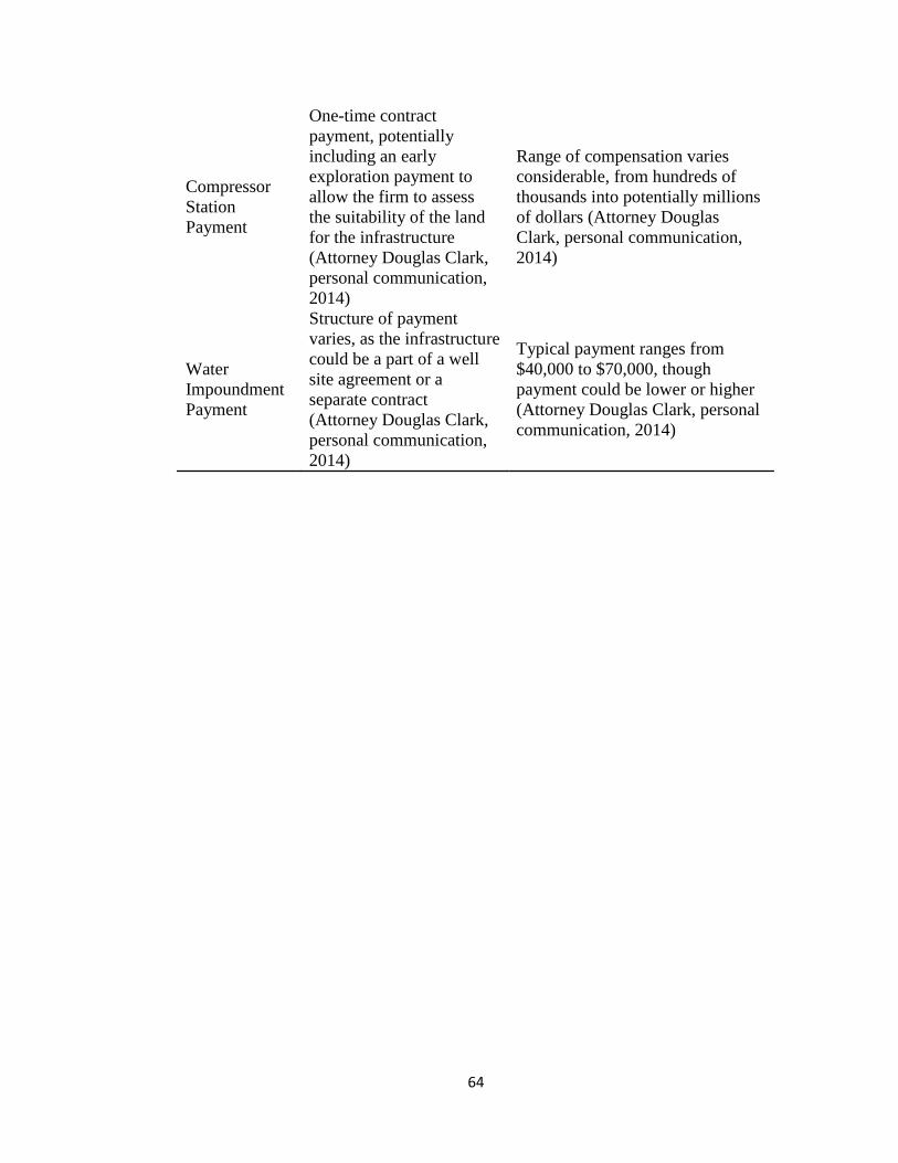
64
Compressor
Station
Payment
One-time contract
payment, potentially
including an early
exploration payment to
allow the firm to assess
the suitability of the land
for the infrastructure
(Attorney Douglas Clark,
personal communication,
2014)
Range of compensation varies
considerable, from hundreds of
thousands into potentially millions
of dollars (Attorney Douglas
Clark, personal communication,
2014)
Water
Impoundment
Payment
Structure of payment
varies, as the infrastructure
could be a part of a well
site agreement or a
separate contract
(Attorney Douglas Clark,
personal communication,
2014)
Typical payment ranges from
$40,000 to $70,000, though
payment could be lower or higher
(Attorney Douglas Clark, personal
communication, 2014)
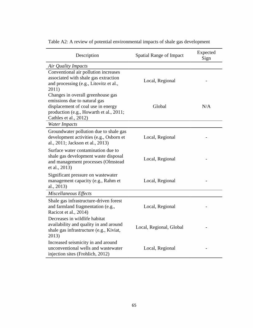
65
Table A2: A review of potential environmental impacts of shale gas development
Description Spatial Range of Impact Expected
Sign
Air Quality Impacts
Conventional air pollution increases
associated with shale gas extraction
and processing (e.g., Litovitz et al.,
2011)
Local, Regional -
Changes in overall greenhouse gas
emissions due to natural gas
displacement of coal use in energy
production (e.g., Howarth et al., 2011;
Cathles et al., 2012)
Global N/A
Water Impacts
Groundwater pollution due to shale gas
development activities (e.g., Osborn et
al., 2011; Jackson et al., 2013)
Local, Regional -
Surface water contamination due to
shale gas development waste disposal
and management processes (Olmstead
et al., 2013)
Local, Regional -
Significant pressure on wastewater
management capacity (e.g., Rahm et
al., 2013)
Local, Regional -
Miscellaneous Effects
Shale gas infrastructure-driven forest
and farmland fragmentation (e.g.,
Racicot et al., 2014)
Local, Regional -
Decreases in wildlife habitat
availability and quality in and around
shale gas infrastructure (e.g., Kiviat,
2013)
Local, Regional, Global -
Increased seismicity in and around
unconventional wells and wastewater
injection sites (Frohlich, 2012)
Local, Regional -
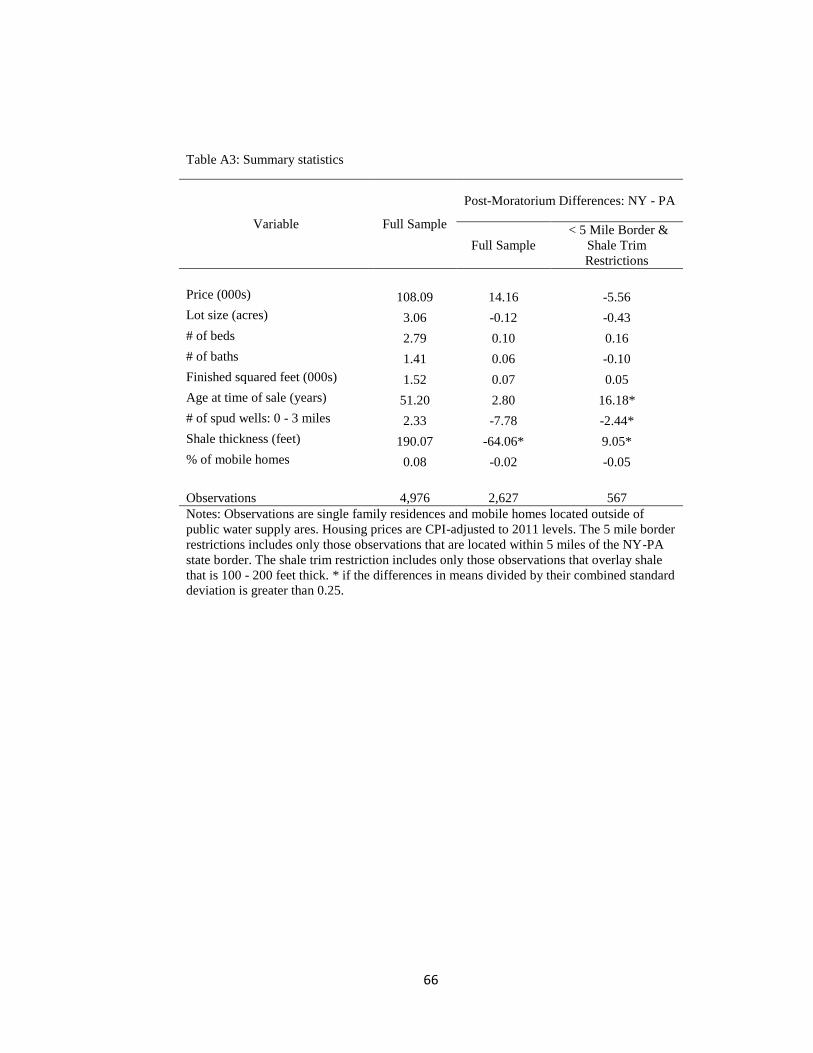
66
Table A3: Summary statistics
Variable Full Sample
Post-Moratorium Differences: NY - PA
Full Sample
< 5 Mile Border &
Shale Trim
Restrictions
Price (000s) 108.09 14.16 -5.56
Lot size (acres) 3.06 -0.12 -0.43
# of beds 2.79 0.10 0.16
# of baths 1.41 0.06 -0.10
Finished squared feet (000s) 1.52 0.07 0.05
Age at time of sale (years) 51.20 2.80 16.18*
# of spud wells: 0 - 3 miles 2.33 -7.78 -2.44*
Shale thickness (feet) 190.07 -64.06* 9.05*
% of mobile homes 0.08 -0.02 -0.05
Observations 4,976 2,627 567
Notes: Observations are single family residences and mobile homes located outside of
public water supply ares. Housing prices are CPI-adjusted to 2011 levels. The 5 mile border
restrictions includes only those observations that are located within 5 miles of the NY-PA
state border. The shale trim restriction includes only those observations that overlay shale
that is 100 - 200 feet thick. * if the differences in means divided by their combined standard
deviation is greater than 0.25.
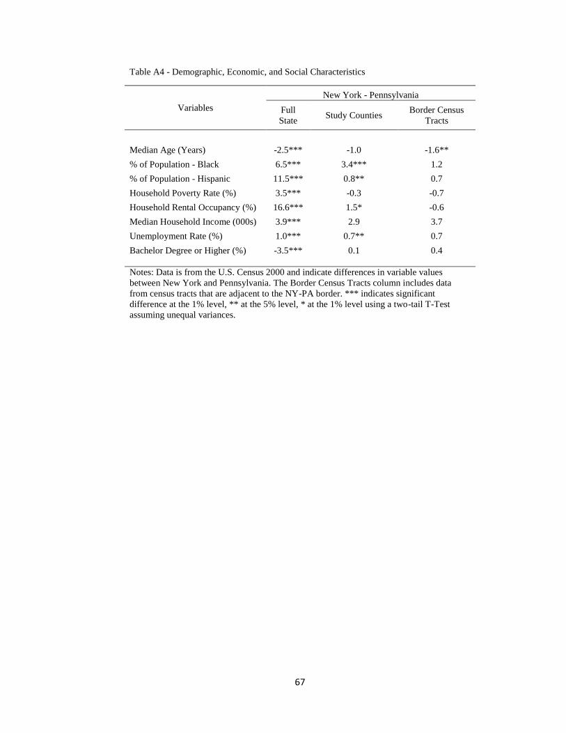
67
Table A4 - Demographic, Economic, and Social Characteristics
Variables
New York - Pennsylvania
Full
State Study Counties
Border Census
Tracts
Median Age (Years) -2.5*** -1.0 -1.6**
% of Population - Black 6.5*** 3.4*** 1.2
% of Population - Hispanic 11.5*** 0.8** 0.7
Household Poverty Rate (%) 3.5*** -0.3 -0.7
Household Rental Occupancy (%) 16.6*** 1.5* -0.6
Median Household Income (000s) 3.9*** 2.9 3.7
Unemployment Rate (%) 1.0*** 0.7** 0.7
Bachelor Degree or Higher (%) -3.5*** 0.1 0.4
Notes: Data is from the U.S. Census 2000 and indicate differences in variable values
between New York and Pennsylvania. The Border Census Tracts column includes data
from census tracts that are adjacent to the NY-PA border. *** indicates significant
difference at the 1% level, ** at the 5% level, * at the 1% level using a two-tail T-Test
assuming unequal variances.
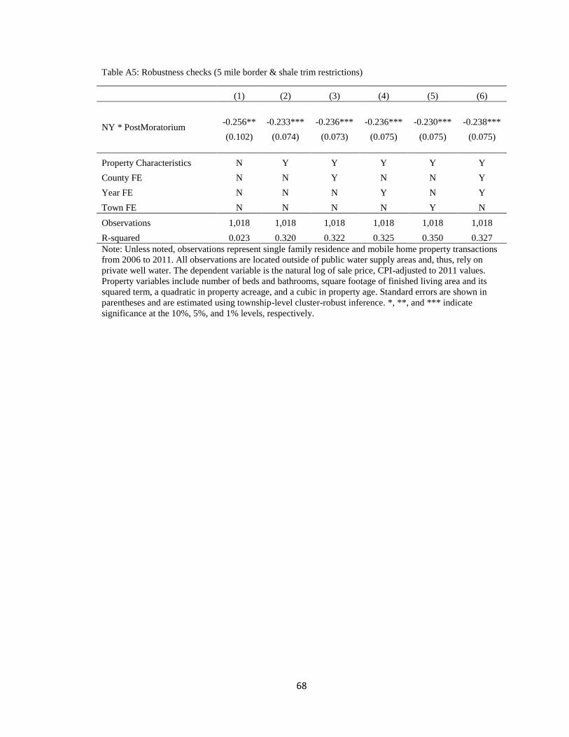
68
Table A5: Robustness checks (5 mile border & shale trim restrictions)
(1) (2) (3) (4) (5) (6)
NY * PostMoratorium -0.256** -0.233*** -0.236*** -0.236*** -0.230*** -0.238***
(0.102) (0.074) (0.073) (0.075) (0.075) (0.075)
Property Characteristics N Y Y Y Y Y
County FE N N Y N N Y
Year FE N N N Y N Y
Town FE N N N N Y N
Observations 1,018 1,018 1,018 1,018 1,018 1,018
R-squared 0.023 0.320 0.322 0.325 0.350 0.327
Note: Unless noted, observations represent single family residence and mobile home property transactions
from 2006 to 2011. All observations are located outside of public water supply areas and, thus, rely on
private well water. The dependent variable is the natural log of sale price, CPI-adjusted to 2011 values.
Property variables include number of beds and bathrooms, square footage of finished living area and its
squared term, a quadratic in property acreage, and a cubic in property age. Standard errors are shown in
parentheses and are estimated using township-level cluster-robust inference. *, **, and *** indicate
significance at the 10%, 5%, and 1% levels, respectively.
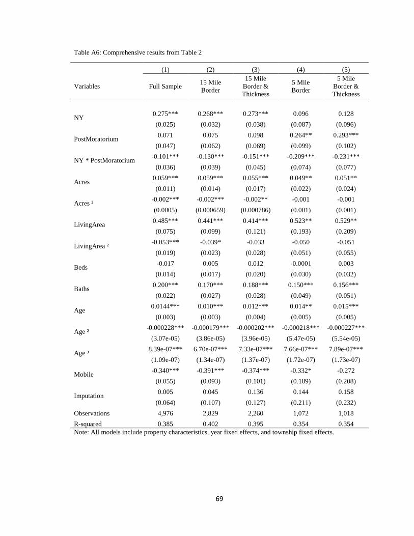
69
Table A6: Comprehensive results from Table 2
(1) (2) (3) (4) (5)
Variables Full Sample 15 Mile
Border
15 Mile
Border &
Thickness
5 Mile
Border
5 Mile
Border &
Thickness
NY 0.275*** 0.268*** 0.273*** 0.096 0.128
(0.025) (0.032) (0.038) (0.087) (0.096)
PostMoratorium 0.071 0.075 0.098 0.264** 0.293***
(0.047) (0.062) (0.069) (0.099) (0.102)
NY * PostMoratorium -0.101*** -0.130*** -0.151*** -0.209*** -0.231***
(0.036) (0.039) (0.045) (0.074) (0.077)
Acres 0.059*** 0.059*** 0.055*** 0.049** 0.051**
(0.011) (0.014) (0.017) (0.022) (0.024)
Acres ² -0.002*** -0.002*** -0.002** -0.001 -0.001
(0.0005) (0.000659) (0.000786) (0.001) (0.001)
LivingArea 0.485*** 0.441*** 0.414*** 0.523** 0.529**
(0.075) (0.099) (0.121) (0.193) (0.209)
LivingArea ² -0.053*** -0.039* -0.033 -0.050 -0.051
(0.019) (0.023) (0.028) (0.051) (0.055)
Beds -0.017 0.005 0.012 -0.0001 0.003
(0.014) (0.017) (0.020) (0.030) (0.032)
Baths 0.200*** 0.170*** 0.188*** 0.150*** 0.156***
(0.022) (0.027) (0.028) (0.049) (0.051)
Age 0.0144*** 0.010*** 0.012*** 0.014** 0.015***
(0.003) (0.003) (0.004) (0.005) (0.005)
Age ² -0.000228*** -0.000179*** -0.000202*** -0.000218*** -0.000227***
(3.07e-05) (3.86e-05) (3.96e-05) (5.47e-05) (5.54e-05)
Age ³ 8.39e-07*** 6.70e-07*** 7.33e-07*** 7.66e-07*** 7.89e-07***
(1.09e-07) (1.34e-07) (1.37e-07) (1.72e-07) (1.73e-07)
Mobile -0.340*** -0.391*** -0.374*** -0.332* -0.272
(0.055) (0.093) (0.101) (0.189) (0.208)
Imputation 0.005 0.045 0.136 0.144 0.158
(0.064) (0.107) (0.127) (0.211) (0.232)
Observations 4,976 2,829 2,260 1,072 1,018
R-squared 0.385 0.402 0.395 0.354 0.354
Note: All models include property characteristics, year fixed effects, and township fixed effects.
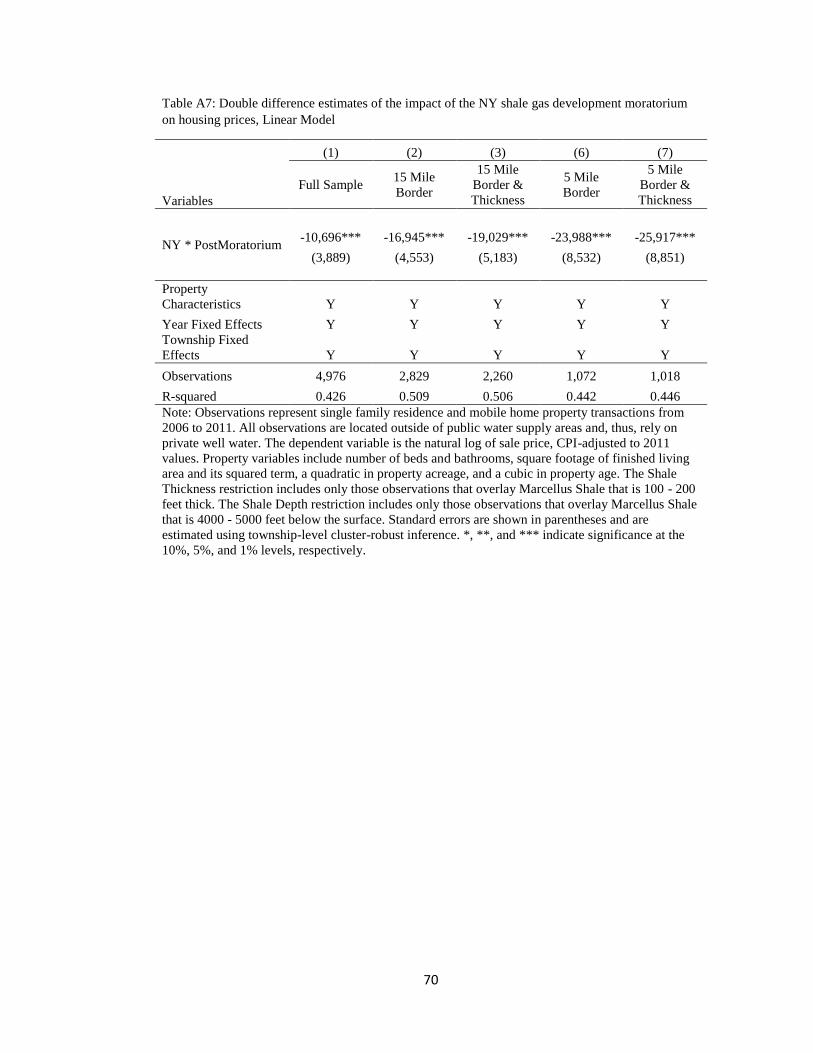
70
Table A7: Double difference estimates of the impact of the NY shale gas development moratorium
on housing prices, Linear Model
(1) (2) (3) (6) (7)
Variables
Full Sample 15 Mile
Border
15 Mile
Border &
Thickness
5 Mile
Border
5 Mile
Border &
Thickness
NY * PostMoratorium -10,696*** -16,945*** -19,029*** -23,988*** -25,917***
(3,889) (4,553) (5,183) (8,532) (8,851)
Property
Characteristics Y Y Y Y Y
Year Fixed Effects Y Y Y Y Y
Township Fixed
Effects Y Y Y Y Y
Observations 4,976 2,829 2,260 1,072 1,018
R-squared 0.426 0.509 0.506 0.442 0.446
Note: Observations represent single family residence and mobile home property transactions from
2006 to 2011. All observations are located outside of public water supply areas and, thus, rely on
private well water. The dependent variable is the natural log of sale price, CPI-adjusted to 2011
values. Property variables include number of beds and bathrooms, square footage of finished living
area and its squared term, a quadratic in property acreage, and a cubic in property age. The Shale
Thickness restriction includes only those observations that overlay Marcellus Shale that is 100 - 200
feet thick. The Shale Depth restriction includes only those observations that overlay Marcellus Shale
that is 4000 - 5000 feet below the surface. Standard errors are shown in parentheses and are
estimated using township-level cluster-robust inference. *, **, and *** indicate significance at the
10%, 5%, and 1% levels, respectively.
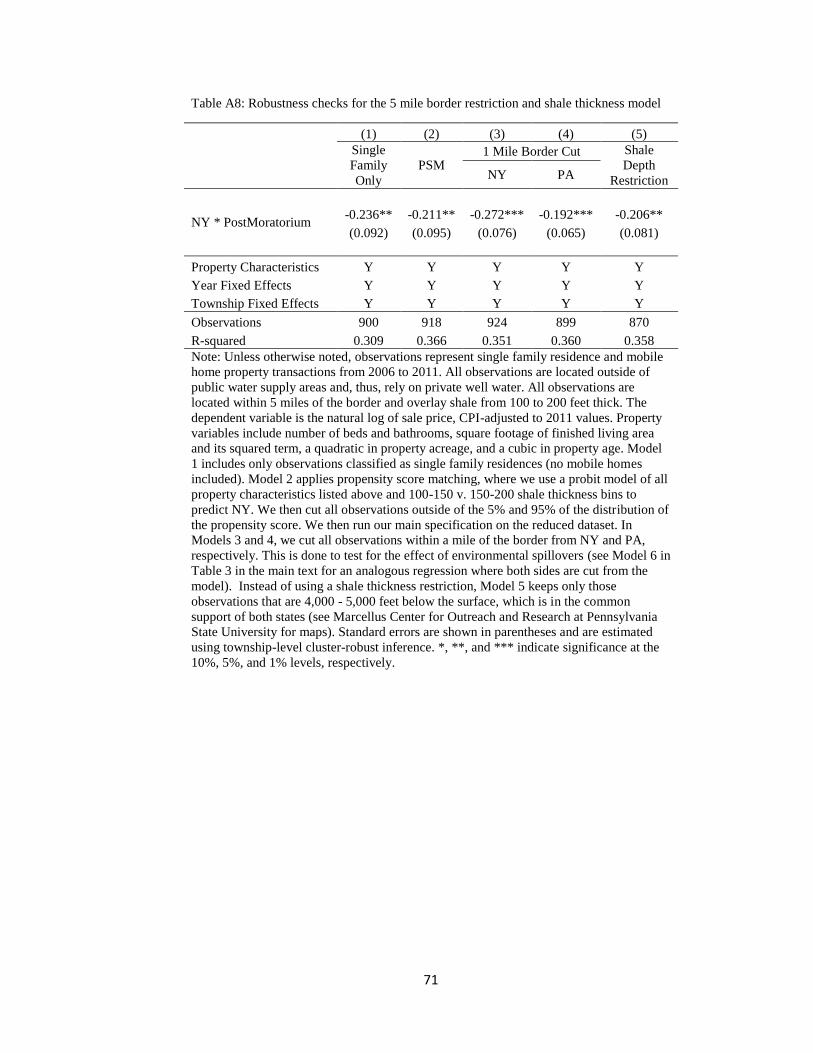
71
Table A8: Robustness checks for the 5 mile border restriction and shale thickness model
(1) (2) (3) (4) (5)
Single
Family
Only
PSM 1 Mile Border Cut Shale
Depth
Restriction NY PA
NY * PostMoratorium -0.236** -0.211** -0.272*** -0.192*** -0.206**
(0.092) (0.095) (0.076) (0.065) (0.081)
Property Characteristics Y Y Y Y Y
Year Fixed Effects Y Y Y Y Y
Township Fixed Effects Y Y Y Y Y
Observations 900 918 924 899 870
R-squared 0.309 0.366 0.351 0.360 0.358
Note: Unless otherwise noted, observations represent single family residence and mobile
home property transactions from 2006 to 2011. All observations are located outside of
public water supply areas and, thus, rely on private well water. All observations are
located within 5 miles of the border and overlay shale from 100 to 200 feet thick. The
dependent variable is the natural log of sale price, CPI-adjusted to 2011 values. Property
variables include number of beds and bathrooms, square footage of finished living area
and its squared term, a quadratic in property acreage, and a cubic in property age. Model
1 includes only observations classified as single family residences (no mobile homes
included). Model 2 applies propensity score matching, where we use a probit model of all
property characteristics listed above and 100-150 v. 150-200 shale thickness bins to
predict NY. We then cut all observations outside of the 5% and 95% of the distribution of
the propensity score. We then run our main specification on the reduced dataset. In
Models 3 and 4, we cut all observations within a mile of the border from NY and PA,
respectively. This is done to test for the effect of environmental spillovers (see Model 6 in
Table 3 in the main text for an analogous regression where both sides are cut from the
model). Instead of using a shale thickness restriction, Model 5 keeps only those
observations that are 4,000 - 5,000 feet below the surface, which is in the common
support of both states (see Marcellus Center for Outreach and Research at Pennsylvania
State University for maps). Standard errors are shown in parentheses and are estimated
using township-level cluster-robust inference. *, **, and *** indicate significance at the
10%, 5%, and 1% levels, respectively.
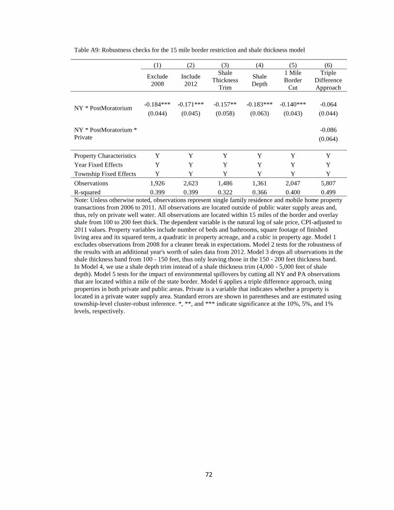
72
Table A9: Robustness checks for the 15 mile border restriction and shale thickness model
(1) (2) (3) (4) (5) (6)
Exclude
2008
Include
2012
Shale
Thickness
Trim
Shale
Depth
1 Mile
Border
Cut
Triple
Difference
Approach
NY * PostMoratorium -0.184*** -0.171*** -0.157** -0.183*** -0.140*** -0.064
(0.044) (0.045) (0.058) (0.063) (0.043) (0.044)
NY * PostMoratorium *
Private
-0.086
(0.064)
Property Characteristics Y Y Y Y Y Y
Year Fixed Effects Y Y Y Y Y Y
Township Fixed Effects Y Y Y Y Y Y
Observations 1,926 2,623 1,486 1,361 2,047 5,807
R-squared 0.399 0.399 0.322 0.366 0.400 0.499
Note: Unless otherwise noted, observations represent single family residence and mobile home property
transactions from 2006 to 2011. All observations are located outside of public water supply areas and,
thus, rely on private well water. All observations are located within 15 miles of the border and overlay
shale from 100 to 200 feet thick. The dependent variable is the natural log of sale price, CPI-adjusted to
2011 values. Property variables include number of beds and bathrooms, square footage of finished
living area and its squared term, a quadratic in property acreage, and a cubic in property age. Model 1
excludes observations from 2008 for a cleaner break in expectations. Model 2 tests for the robustness of
the results with an additional year's worth of sales data from 2012. Model 3 drops all observations in the
shale thickness band from 100 - 150 feet, thus only leaving those in the 150 - 200 feet thickness band.
In Model 4, we use a shale depth trim instead of a shale thickness trim (4,000 - 5,000 feet of shale
depth). Model 5 tests for the impact of environmental spillovers by cutting all NY and PA observations
that are located within a mile of the state border. Model 6 applies a triple difference approach, using
properties in both private and public areas. Private is a variable that indicates whether a property is
located in a private water supply area. Standard errors are shown in parentheses and are estimated using
township-level cluster-robust inference. *, **, and *** indicate significance at the 10%, 5%, and 1%
levels, respectively.
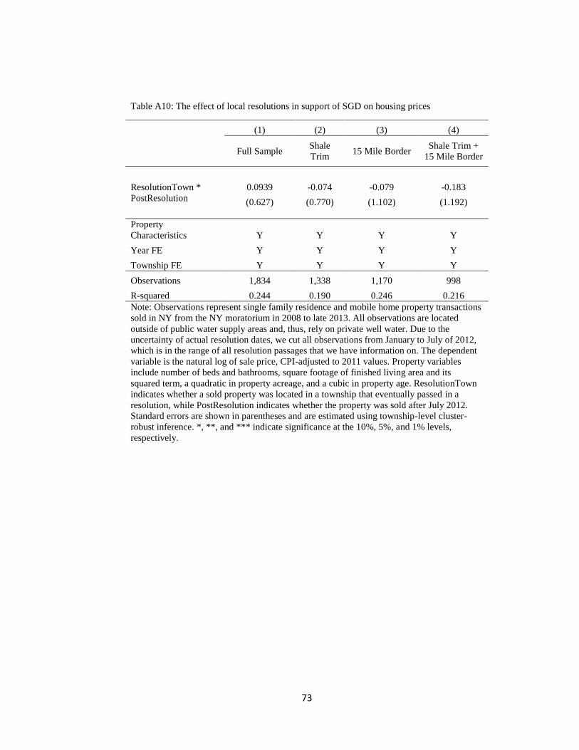
73
Table A10: The effect of local resolutions in support of SGD on housing prices
(1) (2) (3) (4)
Full Sample Shale
Trim 15 Mile Border
Shale Trim +
15 Mile Border
ResolutionTown *
PostResolution
0.0939 -0.074 -0.079 -0.183
(0.627) (0.770) (1.102) (1.192)
Property
Characteristics Y Y Y Y
Year FE Y Y Y Y
Township FE Y Y Y Y
Observations 1,834 1,338 1,170 998
R-squared 0.244 0.190 0.246 0.216
Note: Observations represent single family residence and mobile home property transactions
sold in NY from the NY moratorium in 2008 to late 2013. All observations are located
outside of public water supply areas and, thus, rely on private well water. Due to the
uncertainty of actual resolution dates, we cut all observations from January to July of 2012,
which is in the range of all resolution passages that we have information on. The dependent
variable is the natural log of sale price, CPI-adjusted to 2011 values. Property variables
include number of beds and bathrooms, square footage of finished living area and its
squared term, a quadratic in property acreage, and a cubic in property age. ResolutionTown
indicates whether a sold property was located in a township that eventually passed in a
resolution, while PostResolution indicates whether the property was sold after July 2012.
Standard errors are shown in parentheses and are estimated using township-level cluster-
robust inference. *, **, and *** indicate significance at the 10%, 5%, and 1% levels,
respectively.
74
References
Cathles, Lawrence M., Larry Brown, Milton Taam, and Andrew Hunter, 2012. “A
commentary on “The greenhouse-gas footprint of natural gas in shale formations” by
R.W. Howarth, R. Santoro, and Anthony Ingraffea.” Climatic Change 113(2): 525-
535.
Eichler, Alexander. 2013. “Pennsylvania Fracking: A History of Shale Gas Drilling, as
Told by the People Who Live There.” The Huffington Post, January 25, 2013.
http://www.huggintonpost.com/2013/01/25/pennsylvania-fracking_n_2440227.html
FracTracker. 2014. High Volume Hydrofracking Bans, Moratoria, and Movements for
Prohibitions in New York State. October 9, 2014.
http://www.fractracker.org/map/us/new-york/moratoria/
Frohlich, Cliff. 2012. “Two-Year Survey Comparing Earthquake Activity and Injection-
Well Locations in the Barnett Shale, Texas.” Proceedings of the National Academy of
Sciences, 109 (35): 13934-13938.
Green, Elwin. 2010. “Marcellus Shale Could Be a Boon or Bane for Landowners.”
Pittsburgh Post-Gazette, February 28, 2010. http://www.post-
gazette.com/business/businessnews/2010/02/28/Marcellus-shale-could-be-a-boon-or-
bane-for-land-owners/stories/201002280253
Hefley, William H., Shaun Seydor, Michella K. Bencho, Ian Chappel, Max Dizard,
John Hallman, Julia Herkt, Pei Jiuan Jiang, Matt Kerec, Fabian Lampe,
Christopher L. Lehner, Tingyu Wei, Bill Birsic, Emily Coulter, Erik M. Hatter,
Donna Jacko, Samuel Mignogna, Nicholas Park, Kaitlin Riley, Tom Tawoda,
Eric Clements, and Roman Harlovic, 2011. “The Economic Impact of the Value
Chain of a Marcellus Shale Well.” Working Paper, Katz Graduate School of
Business. University of Pittsburgh. Pittsburgh, PA.
Howarth, Robert W., Renee Santoro, and Anthony Ingraffea, 2011. Methane and the
greenhouse-gas footprint of natural gas from shale formations. Climatic Change
106(4): 679-690.
Jackson, Robert B., Avner Vengosh, Thomas H. Darrah, Nathaniel R. Warner,
Adrian Down, Robert J. Poreda, Stephen G. Osborn, Kaiguang Zhao, and
Jonathan D. Karr. 2013. “Increased Stray Gas Abundance in a Subset of Drinking
Water Wells near Marcellus Shale Gas Extraction.” Proceedings of the National
Academy of Sciences, 110(28): 11250-11255.
Jacquet, Jeffrey, and David L. Kay. 2014. “The Unconventional Boomtown: Updating
the Impact Model to Fit New Spatial and Temporal Scales.” Journal of Rural and
Community Development, 9 (1): 1-23.
Kargbo, David M., Ron G. Wilhelm, and David J. Campbell. 2010. “Natural Gas
Plays in the Marcellus Shale: Challenges and Potential Opportunities.”
Environmental Science & Technology, 44: 5679-5684.
Kelsey, Timothy W., and Thomas B. Murphy, 2011. Economic implications of natural
gas drilling in the Marcellus Shale Region. Federal Reserve Bank of Philadelphia.
Cascade 77.
Kiviat, Erik. 2013. “Risks to Biodiversity from Hydraulic Fracturing for Natural Gas
in the Marcellus and Utica shales.” Annals of the New York Academy of Sciences,
1286: 1-14.
75
Litovitz, Avisa, Aimee Curtright, Shmuel Abramzon, Nicholas Burger, and
Constantine Samaras. 2013. “Estimation of Regional Air-Quality Damages from
Marcellus Shale Natural Gas Extraction in Pennsylvania.” Environmental Research
Letters, 8 (1): 1-8.
Messersmith, Dave. 2010. “Natural Gas Pipeline Right-Of-Ways: Understanding
Landowner Rights and Options.” Report. Penn State Cooperative Extension.
Miller, Timothy, and James M. Sassin. 2014. “Assessing the Impacts of Shale Oil and
Gas Developments on Rural Texas Highway Infrastructure.” Conference Proceeding
Paper. Shale Energy Engineering 2014: Technical Challenges, Environmental Issues,
and Public Policy.
Olmstead, Sheila M., Lucija A. Muehlenbachs, Jhih-Shyang Shih, Ziyan Chu, and
Alan J. Krupnick. 2013. “Shale Gas Development Impacts on Surface Water
Quality in Pennsylvania.” Proceedings of the National Academy of Sciences, 110(13):
4962-4967.
Osborn, Stephen G., Avner Vengosh, Nathaniel R. Warner, and Robert B.
Jackson, 2011. Methane contamination of drinking water accompanying gas-well
drilling and hydraulic fracturing. Proceedings of the National Academy of Sciences
108(20): 8172-8176.
Rabe, Barry G., and Rachel Hampton. 2015. “Taxing Fracking: The Politics of State
Severance Taxes in the Shale Era.” University of Michigan. Center for Local, State,
and Urban Policy Working Paper Series 34.
Racicot, Alexandre, Véronique Babib-Roussel, Jean-François Dauphinais, Jean-
Sébastien Joly, Pascal Noël, and Claude Lavoie, 2014. A framework to predict the
impacts of shale gas infrastructures on the forest fragmentation of an agroforest
region. Environmental Management 53(5): 1023-1033.
Rahm, Brian G., Josephine T. Bates, Lara R. Pertoia, Amy E. Galford, David A.
Yoxtheimer, and Susan J. Riha. 2013. “Wastewater Management and Marcellus
Shale Gas Development: Trends, Drivers, and Planning Implications.” Journal of
Environmental Management, 120: 105-113.
Riely, Kaitlynn. 2014. “Allegheny County Announces Deal for Drilling under Deer
Lakes Park.” Pittsburgh Post-Gazette, March 17, 2014. http://www.post-
gazette.com/local/north/2014/03/17/Fitzgerald-to-discuss-status-of-Marcelluys-Shal
e-drilling-proposal-under-Deer-Lakes-Park-today/stories/201403170148
Schafft, Kai A., Leland L. Glenna, Brandon Green, and Yetkin Borlu. 2014. “Local
Impacts of Unconventional Gas Development within Pennsylvania’s Marcellus Shale
Region: Gauging Boomtown Development through the Perspectives of Educational
Administrators.” Society & Natural Resources: An International Journal, 27 (4): 389-
404.
Weidner, Krista. 2013. “A Landowner’s Guide to Leasing Land in Pennsylvania.”
Pennsylvania State University Cooperative Extension.
76
Manuscript – 2
Submitted to Journal of the Association of Environmental and Resource Economists,
June 2016
Valuation of the External Costs of Unconventional Oil and Gas Development:
The Critical Importance of Mineral Rights Ownership
Andrew Boslett, Todd Guilfoos, and Corey Lang
Environmental and Natural Resource Economics, University of Rhode Island
77
Abstract
This paper seeks to quantify the negative externalities associated with unconventional
extraction of oil and gas using hedonic valuation and residential property transactions.
One complication in determining local impacts is the fact that some but not all properties
are tied with mineral rights, which enable the residents to benefit financially from nearby
drilling. To overcome this issue, we exploit the mineral severance legacy of the Stock-
Raising Homestead Act of 1916 to identify properties in Western Colorado that with
certainty do not have mineral rights and thus are only impacted negatively by proximate
drilling. Our regression results suggest that housing prices decline about 35% when
drilling occurs within one mile. This estimate of local costs is substantially larger than
prior results found elsewhere in the literature, which demonstrates the critical importance
of mineral ownership.
Keywords: unconventional oil and gas development; hydraulic fracturing; horizontal
drilling; federal mineral ownership; mineral severance; hedonic valuation
JEL codes: Q3, Q5
78
1. Introduction
Shale and tight oil and gas basins have emerged as important sources of energy in
the United States through innovations in hydraulic fracturing and horizontal drilling. This
development has led to significant impacts on residents and landowners that are close to
drilling activities. There are environmental and health risks associated with
unconventional oil and gas development related to groundwater contamination (Osborn et
al., 2011), surface water pollution (Olmstead et al., 2013), wastewater management
(Rahm and Riha, 2012), and infant health (Hill, 2013; McKenzie et al., 2014). However,
there are positive impacts as well, especially for those residents that lease their mineral
rights to drilling companies in return for royalty payments and lease signing bonuses
(Fitzgerald, 2014; Hardy and Kelsey, 2015).1 Royalty payments can be paid as high as
20% of the value of production and lease signing bonuses can reach into the thousands of
dollars per acre leased (e.g., Brasier et al., 2011; Kelly-Detwiler, 2013).
There is a growing body of literature in economics that seeks to estimate the local
impacts of unconventional oil and gas development through hedonic valuation, with
remarkable variation in estimates. Gopalakrishnan and Klaiber (2014) examine price
responses in southwestern Pennsylvania and find that prices can decline by as much as
22% for private well-water dependent properties, but generally are smaller and short
lived. Muehlenbachs et al. (2015) use data from across Pennsylvania and find that shale
development can lead to depreciation as high as 17% for well water properties within 1.5
1 The United States is unique in that private citizens can own the minerals underneath their property. In
most countries, it is the government or the crown that owns all subsurface rights (Kulander, 2013). Since
U.S. citizens can own their properties’ minerals, they can financially benefit from drilling through leasing.
The possibility of financial benefits has led to more public support for unconventional oil and gas
development in the United States than in other countries (e.g., Stevens, 2010; Gény, 2010). Private mineral
rights ownership has been crucial in driving development in the United States (Wang and Krupnick, 2013).
79
kilometers of an unconventional drill site. They also find that drilling can have a small
positive impact on property sale prices in public water supply areas. Delgado et al. (2016)
use data from Northeastern Pennsylvania and find no robust impact of nearby drilling.
Boslett et al. (2016) examine the impact of the New York State moratorium on
unconventional drilling and find New York properties most likely to be impacted by
shale gas development declined 24% in value relative to comparable Pennsylvania
properties after the moratorium. They interpret this finding as a positive expected value
of shale gas development. Weber and Hitaj (2015) find evidence of appreciation in farm
property values in both Pennsylvania and Texas, especially during leasing periods.
Importantly, their estimates are attenuated in areas with significant mineral severance. In
Colorado, Bennett and Loomis (2015) find mixed results that are often not statistically
significant. Also in Colorado, James and James (2015) find that a one kilometer decrease
in distance away from an unconventional well is associated with a 7 to 20% decrease in
sale price. However, this effect can be mitigated if the property is above a horizontal well
lateral, which suggests royalty payments from leasing are capitalized into prices. Using
zip code level aggregate data from Texas, Weber et al. (2016) find evidence of both
appreciation and depreciation due to shale development. There remain large variations in
estimates of shale gas development on property prices without sufficient explanation.
One potential reason for the contrasting results is that mineral right ownership is
not accounted for explicitly in these studies. Mineral ownership is important because it
firmly demarcates property owners who financially benefits from unconventional gas
development versus those who do not. Without mineral ownership information, it is not
known whether the recovered valuation is a net impact of financial positives and
80
environment/health negatives, purely the negatives, or a weighted average of the two. In
Pennsylvania, which is the focus of several of the above studies, mineral right ownership
varies substantially and systematically across the state. In Western Pennsylvania, where
there is a legacy of energy extraction, mineral rights are more often severed from surface
rights than in northeastern Pennsylvania, where energy extraction only started recently
(Kelsey et al., 2012). The valuation studies focused on Eastern Pennsylvania estimate less
negative (or even positive) impacts of shale gas.2 While the important distinction between
private well water and public water properties has been identified by the existing hedonic
valuation literature, the critical issue of mineral rights ownership has not been resolved.
This has not been a lack of foresight or understanding by researchers of the importance of
mineral ownership in how people are impacted by drilling. Rather, this information is
extremely difficult for researchers to obtain.3
In this paper, we resolve the issue of unknown mineral rights by exploiting a
historical severance in mineral rights ownership, the Stock-Raising Homestead Act of
1916 (SRHA1916). Over the course of the 19th century, the United States expanded its
boundaries through territorial acquisition, often exchanging land rights for homesteading
starting with the Homestead Act of 1862. In the late 1800s and early 1900s, the federal
2 Consistent with this interpretation of the valuation results, homeowners that do not own mineral rights
have an increased perception of environmental risk (Brasier et al., 2013) and frustration (Collins and
Nkansah, 2015). 3 Mineral right ownership information is held in county deeds offices and is not commonly included in
property deeds. The chain of title can be unclear, especially when the mineral estate was historically
separated from the surface estate. One may need to go back to the original land grant to confirm the title of
the mineral estate. Charting mineral rights ownership over time is the full-time job of a title abstractor
(Wilson, 2014). Suffice it to say, it would be difficult for researchers to successfully obtain mineral rights
ownership information for a large property transaction database. One of the authors of this study spent a
day at Pennsylvania’s Bradford County’s Register and Recorder office researching mineral rights transfers
and can attest to this. See Table 1A in the Appendix on a review of the previous literature and how each
paper contextualized the issue of mineral rights ownership.
81
government recognized both the increasing value of energy for economic growth and the
government’s inability to properly identify “mineral” lands, which they kept in federal
ownership, and “nonmineral” lands, which they disbursed for homesteading. In response,
the federal government passed the SRHA1916, which continued the tradition of land
disbursement, but the federal government retained ownership of minerals in all land
disbursed after 1916 (Gates, 1977; Harrison, 1989).
To build our dataset of transactions, we identify residential properties in Colorado
located on land originally distributed under the SRHA1916. Thus, the federal government
owns the mineral rights for each of these properties and current residents do not benefit
financially from lease and royalty payments. Our study area is on the western slope of
Colorado, centered in Garfield, Mesa, and Rio Blanco counties. Western Colorado was
one of the major areas of post-1916 homesteading and this region is one of the primary
locations of unconventional oil and gas development in the state.
Our hedonic analysis suggests that houses within one mile of an unconventional
drill site sell for 34.8% less than comparable properties without proximate drilling. This
result is robust across various subsets of the data and alternative regression specifications,
including a repeat sales model and a matching model. When multiplied by the average
house price of $183,300, this discount translates to a price reduction of $63,788, which
equals $3,952 when annualized by a 30-year mortgage and a 5% interest rate. We
interpret this price difference as the household valuation of the external environmental
and health costs associated with proximity to unconventional oil and gas development.
Our findings corroborate the negative valuations found in other papers, but are
much larger – 60% larger in magnitude than the largest existing negative estimate. This
82
disparity demonstrates the importance of understanding mineral rights, as financial
benefits of drilling are capitalized into housing prices and can adulterate estimates of
external costs. Supporting this conclusion, we also estimate hedonic models using
Western Colorado properties with unknown mineral rights ownership, mirroring the setup
of prior studies, and find much smaller and statistically insignificant impacts of
proximity.
Our paper is structured as follows. We start in Section 2 with a conceptual
framework that discusses the issue of mineral rights ownership in valuation of
unconventional oil and gas development. In Section 3, we outline the history of
SRHA1916. In Section 4, we discuss our data set and how we obtained it. We then follow
with a discussion our methodological approach and the assumptions we use in our
interpretation of our model results. In Section 5, we present our results, and Section 6
concludes.
2. Conceptual Framework
In this section, we outline the potential biases in hedonic valuation of
unconventional oil and gas development. The net benefits and costs of oil and gas
development vary across mineral estate classifications. Only residential properties that
are unified with their property’s mineral estate can receive direct financial benefits, such
as a lease signing bonus and production-based royalties. However, all properties receive
the environmental costs of nearby oil and gas development. Previous hedonic valuation
work has not incorporated the ownership of mineral rights into valuation frameworks due
83
to the lack of data. Thus, these studies have typically contextualized their estimates as net
valuations of local oil and gas development. 4
We define the price of property i as )(iP , a function of environmental
characteristicsiE , the financial benefits of oil and gas development
iF , and structural
characteristics. The environmental quality of the property is influenced by the presence of
local oil and gas development, iD . These impacts could be associated with diminished
water quality, air quality, forest and habitat fragmentation, or visual or noise
disamenities. Additionally, the financial benefits of owning the property are impacted by
the presence of local oil and gas development,iD .
In this framework, mineral ownership is defined as a binary variable,iM , equal to
1 if the property’s surface estate is connected with its mineral estate and equal to 0
otherwise. The net valuation of unconventional oil and gas development for property i
can be decomposed as follows:
(1) i
i
i
i
i
i
i
i
i
iD
F
F
PM
D
E
E
PValuation
Thus, the valuation of development, as capitalized by housing prices, is a net valuation of
the environmental impacts of development (first term) and the financial benefits of
development, contingent on ownership of the property’s mineral estate (second term). For
the sake of simplicity, we re-write the equation as:
(2) BMCValuation ii ,
4 Muehlenbachs et al. (2015) note that their estimate of the adjacency effect is an overall effect of the
financial benefits of nearby drilling minus its environmental costs, while Gopalakrishnan and Klaiber
(2014) remark that their negative valuations are likely understated due to the fact that they cannot control
for the potential benefits of mineral leasing.
84
where C and B refer to the true values of the capitalization of the financial benefits and
environmental costs (Table 1). If a property has mineral rights, then the estimated
valuation will be the net impact, BC . However, if a property is a split estate, then the
estimated valuation will be the external costs of being proximate to drilling.
In order for researchers to estimate valuation with real data, a residential property
market level analysis is required. We define as the proportion of properties unified with
their minerals. Using the terminology from Table 1, we have:
(3) )1()( CBCValuationEstimated
The estimated valuation is conditional on the proportion of treated properties with
mineral rights, which is unknown to the researcher. Knowing either BC or C is useful
for understanding local impacts and for guiding policy. But a weighted average of the
two with an unknown weight yields imprecise guidance.
In this paper, we take advantage of the historical split in mineral rights from
surface rights caused by SRHA1916, which is detailed in the next section. Thus, in our
sample, = 0 and we can isolate the negative environmental costs, C, from the financial
benefits of development. This framework assumes there are no area level impacts of oil
and gas development on properties which differ by mineral rights ownership, which
would impact the estimate of proximity to wells. This potential issue is easily addressed
with information about mineral rights ownership over the entire population of sale, or
restricting the sample to only those properties without mineral rights ownership, i.e. =
0, as we do in this study.
3. The Stock-Raising Homestead Act of 1916
85
In the late 1800s and early 1900s, the federal government passed a series of
homestead acts that encouraged immigration and development in the western United
States. The exact mandate varied across the acts; typically, settlers received 160-640
acres in return for a promise of ranching, cropping, or timber management on the
property (Bureau of Land Management, 2006).
Early homestead acts apportioned both surface and subsurface rights to
homesteaders. This was the case for the original Homestead Act of 1862, signed by
President Abraham Lincoln after the separation of the Confederacy from the United
States. These lands were selected for disbursement due to their perceived “nonmineral”
character, as delineated by General Land Office’s entrymen and surveyors. All lands with
mineral potential were retained by the federal government; however, demarcation was
imperfect due to technology limitations (Leshy, 1987).
Recognizing its limitations in mineral assessment, the federal government passed
the SRHA1916. This policy effectively discontinued the mineral-nonmineral
classification system (Harrison, 1989). Homesteading individuals were granted no more
than a section of land for ranching and forage crop production, conditional on making
permanent improvements on the land within three years of the entry date. However, the
federal government would retain mineral ownership of all lands disbursed through the
Stock-Raising Homestead Act:
“That all entries made and patents issued under the provisions of this Act shall be
subject to and contain a reservation to the United States of all coal and other
86
minerals in the lands so entered and patented, together with the right to prospect
for, mine, and remove the same.”5
In addition, homesteaders and other later surface right owners had to allow access
to the land for subsurface exploration and production:
“Any person who has acquired from the United States the coal or other mineral
deposits in any such land, or the right to mine and remove the same, may reenter
and occupy so much of the surface thereof as may be required for all purposes
reasonably incident to the mining or removal of the coal or other minerals, first,
upon securing the written consent or waiver the homestead entryman or patentee;
second, upon payment of the damages to crops or other tangible improvements to
the owner thereof…or, third, in lieu of either of the forgoing provisions, upon the
execution of a good and sufficient bond…to secure the payment of such damages
to the crops or tangible improvements of the entryman or owner.”6
This condition precludes the surface owner from preventing mineral exploration.
The intent of the act was to continue the practice of homesteading and agricultural
development of the west without compromising the federal government’s interest in
mineral exploration (Tanke and Putz, 1982). If the surface owner had the right to prevent
production from the property, the mineral estate would have no value. More recent
5 The Statues at Large of the United States of America from December, 1915 to March, 1917. Session 2.
Chapter 9. Section 9. Page 864. 6 The Statues at Large of the United States of America from December, 1915 to March, 1917. Session 2.
Chapter 9. Section 9. Page 864.
87
legislation has maintained surface use access for mineral rights interests while providing
some limited protection to surface owners through accommodation doctrine. This
principle allows only “reasonable” use of the surface by the mineral owner. The mineral
owner may only access the surface if there are no other alternatives that could avoid
interference with the present surface uses (Johnson, 1998). However, mineral rights
dominance has largely been kept in place, as it is difficult for surface owners to prove
that the use of the surface by the mineral owner is not reasonable (Kulander, 2013).
On privately-owned lands with federal mineral ownership, the mineral lessee
must make a “good faith effort” to secure surface owner consent to access the property
(Bureau of Land Management, 2007). However, the surface estate owner is only entitled
to compensation associated with damages to crops and agricultural-related improvements.
Thus, in the context of shale gas extraction, a homeowner may be exposed to water
contamination, air pollution, noise, and visual disamenities, but not be entitled to
compensation.7
The SRHA1916 led to a significant amount of private land with federal mineral
ownership in the western United States. Out of approximately 300 million acres
conveyed to private individuals through the various homesteading acts (Loomis, 2002),
nearly 60 million acres have been split from their underlying subsurface estates as a result
of the SRHA1916. In Colorado alone, these lands total 5.2 million acres. Figure 1 shows
lands with federal mineral ownership across Colorado.
In a split estate, the surface property owner cannot financially benefit from
7 If the mineral lessee cannot come to a surface use agreement with the land owner, the company must rely
on a performance bond to indemnify against unforeseen damages to crops and agricultural improvements.
However, this bond does not cover all damages that a surface owner may face from drilling.
88
drilling. This situation is common in areas of the country that have experienced historical
energy development and mining (e.g., Kelsey et al., 2012; Pender et al., 2014; Railroad
Commission of Texas, 2015). Surface ownership can be split from its mineral rights
through the issuance of a severance deed, in which a private landowner sells the land but
retains the minerals. This situation is analogous to mineral ownership law in other
countries: private land owners neither control the course of oil and gas development, nor
financially benefit from it. The mineral estate is essentially dominant, which means that
the surface owner must allow access to the mineral owner for exploration.
4. Empirical Setting and Data
Colorado has a long history of oil and gas development. According to data from
the U.S. Geological Survey (Biewick, 2008), most Colorado counties have experienced
oil and gas exploration since the early 1900s. Some counties, especially those outside of
the intermountain areas, have seen a large increase in oil and gas development since the
1940s.
More recently, the new technologies of horizontal drilling and hydraulic
fracturing have been used for extraction in Colorado. According to Drillinginfo, over
11,000 horizontal wells were drilled in Colorado between 2000 and 2014. Figure 1
displays the spatial distribution of this drilling. There are generally three drilling
hotspots: northwestern Colorado, Weld County on Colorado’s Front Range, and La Plata
and Montezuma counties in southwestern Colorado. Our study focuses on northwestern
Colorado because there is extensive federal mineral ownership in this area. Bennett and
89
Loomis and (2015) and James and James (2016) examine impacts in Weld County, which
is more densely populated, but has much less federal mineral ownership that
northwestern Colorado. Montezuma County contains many tribal lands, which
complicates analysis due to jurisdictional complexity of mineral development and policy
(West, 1992).
In this study, we use residential property transaction data from Garfield, Mesa,
and Rio Blanco counties in western Colorado. We received this data from each county
assessor’s office. All transactions in our analyses occurred from 2000 to the end of 2014.
All transaction data contains property characteristic information including the number of
bedrooms and bathrooms, living area, age of the property, and its classified property or
land use. We include only those transactions that are defined as residential or agricultural
with a residential building (N = 55,114). All mobile homes are dropped from the analyses
(N = 2,819).8 The data allow us to observe multiple sales per property, not just the most
recent. All transactions that had more than seven bedrooms were dropped out of concern
that the properties were apartment buildings (N = 16).
In order to focus on properties without mineral rights, we use the federal mineral
ownership data from the Bureau of Land Management’s Colorado GIS office.9 We
overlay federal oil and gas ownership data layers with parcel boundaries. We include
properties in our final sample that are completely contained within the federal mineral
ownership boundaries (N = 871).10 While this cuts 98% of the transactions in our
8 Results from our main models are robust to including mobile homes and are available in the online
appendix. 9 “Statewide Federal Mineral Ownership” data product. 10 There were data scale and alignment issues between our parcel data and our mineral ownership data. As a
result, our restriction is conservative. There are likely other properties that are severed from their oil and
gas rights by the SRHA but are not fully within the federal mineral ownership extent. We test our results
90
database, this restriction is necessary to identify the subset of properties that do not
benefit financially from nearby drilling. It is almost certain that some properties outside
of the federal mineral ownership boundary do not own mineral rights, but it is unknown
on a property basis. Thus, this is the sample that provides the best estimate of the external
costs of local oil and gas development. As shown in the results section, our coefficient
estimates change considerably when we include properties with unclear mineral rights
ownership. Lastly, we cut all observations in the below the 5th and above the 95th
percentile of the sale price distribution to remove the influence of outliers. Our final
sample is 783 transactions.
We received directional and horizontal well development data from Drillinginfo.
In our three counties, there were 4,374 horizontal wells drilled from 2000 to 2014. Figure
2 maps the distribution of these wells relative to federal mineral ownership. In ArcGIS,
we calculate the distance to the closest well at the time of sale. In addition, we calculated
additional spatial statistics associated with distance to the closest municipality (U.S.
Census definition) and the percentage of the property in an agricultural use from the
National Land Cover Dataset 2001 to use as control variables in our regression model.
Table 2 provides summary statistics for our preferred sample of split estate
properties, as well as the complete set of properties. Properties with federal mineral
ownership are less expensive, relative to the population of properties. Split estate
properties typically are less expensive, are larger in lot size, and have relatively less
agricultural land. Interestingly, split estate properties are also more likely to have a
using less restrictive definitions of a split estate (i.e., 75 and 90% of property within federal mineral
ownership boundary) and find robust results (available in the online appendix).
91
nearby horizontal well.11
As discussed in the introduction, prior hedonic valuation papers have focused on
differences in impacts between municipal water and private well water properties
(Gopalakrishnan and Klaiber 2014, Muehlenbachs et al. 2015, Boslett et al. 2016). In
Colorado, data does not exist on which properties have private vs. public water supply.
However, our primary sample of split estate properties are typically outside of municipal
boundaries, which is the best proxy for public water supply.12 Therefore, our estimates
are applicable to households that face the risk of groundwater contamination and are
comparable to studies that focus on private water properties.
5. Methodology
We use the hedonic price method to estimate the effect of drilling proximity on
housing prices. Our basic specification is:
(4) isttsististist XWellp ')ln( .
istp is the sale price of property i in spatial unit s in year t. Prices are adjusted to 2015
levels using the Consumer Price Index. istWell is a binary variable that indicates whether
property i has an unconventional well within a given distance buffer at the time of sale.
'
istX is a vector of structural, locational, and environmental explanatory variables. s are
spatial fixed effects; we present specification using both county and census tract as the
11 This may suggest that there is a relationship between well development and mineral right severance, but
that is beyond the scope of this paper. 12 Phone conversation with Scott McGowan, GIS Coordinator with the Colorado Department of Public
Health and Environment).
92
spatial unit. t are year fixed effects. Collectively, these fixed effects control for
unobserved price determinants across space and time. ist is the error.
is our coefficient of interest and is interpreted as the impact of having an
unconventional well within r miles of the property on residential sale prices. Since we are
only analyzing properties with federal mineral ownership, it reflects the marginal value of
the environmental costs of having an unconventional well within the given spatial buffer.
Our goal is to define the radius r so that it captures the full spatial extent of
negative externalities, but this is a priori unknown. Following Linden and Rockoff
(2008) and more recently Muehlenbachs et al. (2015), we estimate a version of Equation
(4) that includes a series of binary variables for different distance bands and seek to
determine empirically at what distance the impact is statistically zero.
Figure 3 graphically presents results of a model that regresses log sales price on
half mile distance bandwidths out to two miles, as well as property characteristics, year
fixed effects, and census tract fixed effects. Results suggest that parameter estimates for
the 0-0.5 mile bin and 0.5-1 mile bin are negative and statistically significant. Coefficient
estimates are statistically insignificant beyond one mile. This finding is robust across
alternative distance bin classifications and similar to findings from Gopalakrishnan and
Klaiber (2014) and Muehlenbachs et al. (2015), who use a one mile and a two kilometer
buffer, respectively, in their analyses. The similarity in coefficient estimates between the
0-0.5 mile and 0.5-1 mile bins is at first surprising because we would expect greater
externalities closer to the drill sight. However, Figure 3 also displays the frequency of
observations by distance and we see clustering of observations around 0.5 miles, which is
why it is difficult to discern differential impacts less than and greater than 0.5 miles.
93
Going forward, we define r equal to one, and hence istWell is a binary variable equal to 1 if
there was a well drilled within one mile of the property before its sale.
5.1 Assumptions
There are a number of assumptions needed to interpret our estimates as the
valuation of the environmental costs of unconventional oil and gas development. First,
we assume that the assignment to treatment – in this case, close proximity to a horizontal
well – is exogenous. It is unlikely that split estate owners can strongly dictate whether
drilling happens, as the surface owner cannot prevent the mineral estate owner from
accessing subsurface resources. Impacted parties can protest the inclusion of a parcel in
an oil and gas lease sale (Bureau of Land Management Regulation 43 CFR 3120.1-3), but
we were unable to find any protests directly from homeowners in our three study
counties.13 A potential concern is that early oil and gas development could influence the
likelihood of severance. In our case, the likelihood of severance is not a concern because
of our study area’s historical severance of mineral rights.
Second, we assume that property buyers and sellers have full information about
local drilling activity and its potential for environmental impact. This is reasonable given
the scale of planning and land disturbance associated with well permitting and drilling
(e.g., Moran et al., 2015) and significant local discussion regarding the impacts of drilling
(e.g., Williams, 2008; Lustgarten, 2009; Harmon, 2014). This region of Colorado has
13 There are examples of homeowners protesting the inclusion of a parcel in a 2012 lease sale in Delta
County, outside of our study area. Most protests submitted to the Bureau of Land Management concerned
environmental and social issues associated with drilling on publically-owned land, not split estate concerns
on privately-owned land.
94
also been the primary site for multiple assessments of the health risks associated with
unconventional development (e.g., Kassotis et al., 2013). As a result, home buyers are
likely conscious of the potential benefits and costs of unconventional oil and gas
development.
Third, property buyers and sellers are informed of the property’s mineral right
status and they understand its ramifications. There has been significant mineral
development in western Colorado over the last century (Biewick, 2008). As a result,
citizens are likely familiar with both oil and gas development and mineral ownership
laws. The state legislature also passed a law in 2001 that required pre-transaction
notification of the potential for a split estate (Garfield County Energy Advisory Board,
2007). There has been much public discussion since 2000 regarding a law that would
mandate disclosure of mineral severance prior to all real estate sales. Although this
legislation has not been passed due to issues secondary to the disclosure requirement
(Moreno, 2011), it has been a major point of policy discussion in the state legislature over
the study’s time period. Additionally, federally-owned minerals were never disbursed
with the land, so a title search is relatively quick and the information is publically
accessible on the Bureau of Land Management’s website.
Fourth, we assume that our estimates are not impacted by positive spillover
effects of unconventional oil and gas development, including labor opportunities and
improved public finances. Although these can be important benefits of local oil and gas
development (e.g., Weber, 2012; Newell and Rami, 2015), these benefits are likely to be
received at the regional level and are unlikely to be related to drilling adjacency or to
mineral rights ownership.
95
Fifth, we assume that the financial benefits that a split estate owner can receive
from local development are negligible. Landowners who do not own mineral rights are
unable to receive lease or royalty payments from on-site production. However,
landowners can receive compensation through a surface use agreement, which formally
outlines where drilling and surface disturbances can happen on the property. Drilling
companies must make a “good faith effort” to come to a surface use agreement with a
landowner in a split estate situation. If the two parties are unable to come to an
agreement, then the drilling company can rely on a performance bond (Bureau of Land
Management, 2007). This alternative option does not cover all damages that a surface
owner may face from drilling, such as contaminated drinking water, drilling-related
noise, air pollution, and visual changes to the landscape. Additionally, performance
bonds are typically meant to compensate for damages to cropland, but not pastureland
(Fitzgerald, 2010). Since lands subject to SRHA1916 were originally intended for
ranching and were deemed largely unsuitable for cropping, it is unlikely that property
owners are reliant on a performance bond to indemnify them against damages related to
drilling. It is more often than not that the surface owner will come to a surface use
agreement with the drilling lessee (Hill and Rippley, 2004; BLM, 2006; Fitzgerald,
2010). Anecdotal reports suggest that oil and gas developers have leverage in
negotiations, as they can rely on a performance bond if they do not agree to the surface
owner’s preferred terms (e.g., The Telluride Daily Planet, 2005; Powder River Basin
Resource Council, 2010; Hancock, 2014). For these reasons, it is unlikely that the
financial benefits accrued from signing a surface use agreement are significant.14
14 This was corroborated in an email conversation with Cameron Grant, a mineral law attorney (Lyons
Gaddis Kahn Hall Jeffers Dworak & Grant, A Professional Corporation of Attorneys and Counselors).
96
5. Results
5.1 Main Results
In Table 3, we present results that estimate the parameters of Equation (4),
defining istWell as a binary variable equal to 1 if there was a well drilled within one mile
of the property. We present four model specifications that sequentially add more control
variables to the model. Column 1 only includes property and location variables (i.e.,
number of bedrooms, distance to closest municipality), Column 2 adds year fixed effects,
Column 3 adds county fixed effects, and Column 4 replaces county fixed effects with
census tract fixed effects. Across columns, the coefficient on proximity ranges from -
0.211 to -0.362 and is always statistically significant. The coefficient increases in
magnitude substantially when year fixed effects are included, which is intuitive given that
drilling (and hence treatment) is correlated with time. The coefficient is stable across
Columns 2-4. Our preferred model is Column 4 that includes both year and tract fixed
effects. This specification indicates that houses within one mile of an unconventional
well sell for 34.8% less than houses further away, all else equal. This discount for
proximity when multiplied by the average house price of $183,300 translates to price
reduction of $63,788. Converting this into an annual impact using a 30-year mortgage
and a 5% interest rate yields $3,952, which is our best estimate of the annual external
impacts of unconventional oil and gas development.
97
5.2. Robustness checks
In Table 4, we test for the robustness of this general result across alternative
specifications and subsets of the data. In Column 1, we include an additional control
variable, which is the number of vertical (conventional) oil and gas wells drilled within a
mile of a property between 1980 and 1999. The concern is that past drilling is likely
correlated with unconventional drilling, and thus if there is a negative impact on prices of
past drilling, our estimates in Table 3 could be misattributing the variation from past
drilling to current drilling. Since recent vertical well development may be an exploratory
precursor to later horizontal well development, we use pre-2000 data to avoid potential
endogeneity issues. In Column 2, we restrict our sample to only properties that are within
20 miles of an eventual unconventional well site. One concern with our full sample used
in Table 3 is that some observed sales are far from drilling and may be a poor control
group. By restricting the spatial distance, we hope to mitigate any bias that results from
distant control observations. Column 3 further restricts the sample to be within 10 miles
of an eventual unconventional well site. In Column 4, we restrict observations to be
within 2005 to 2014. No proximate drilling took place within one mile of any sample
properties prior to 2005. In our full sample, these pre-2005 properties are purely control
observations. If there are structural changes in the housing market not captured by year
fixed effects, then these observations may not be a good control and our estimates may be
biased. In Column 5, we exclude all observations that sold more than once over our time
period. Although fifteen years is a long time, there may be unobservable differences in
the price dynamics of properties that sold multiple times over the study’s period. In
98
Column 6, we estimate a repeat sales model and include only properties that sold more
than once. Including property-level fixed effects better controls for unobservable property
characteristics that could be correlated with proximity to drilling.
The coefficient estimates across these six columns are largely consistent with the
main results. Magnitudes range from -0.307 to -0.381 and all estimates are statistically
significant. Table 4 indicates that our estimates of the effect of drilling with one mile of a
residential property are largely robust to alternative specifications and subsets of the
data.15
5.3. Matching analysis
In this section, we shift to a matching approach in order to better control for
observable differences between our control and treatment groups (e.g., Abbot and
Klaiber, 2013; Ghanem and Zhang, 2014; Ferraro et al., 2015). The main goal of
matching is to avoid the issue of selection bias and to create valid treatment-control
comparisons through pairing on observable covariates (e.g., Caliendo and Kopeinig,
2008; Angrist and Pischke, 2009). This occurs when the estimated relationship between
treatment status and outcome is driven by inherent differences in covariate distributions
between treatment and control groups.
We use matching to further test the robustness of our regression model results.
15 In the Appendix, we provide additional robustness checks. In Tables 2A and 3A, we find qualitatively
similar results when we define our treatment variable as the number of wells drilled within one mile of the
property’s extent, or when we use a distance bin approach. At the suggestion of a reviewer, we estimate our
models in levels, as opposed to logs, and find similar results (Table 3A). In line with the structure of Table
4, we provide additional robustness check in Table 5A. All results from the Appendix support our main
findings.
99
We first estimate a propensity score model of the probability of treatment as a function of
property-specific variables:
(5) ititit XWell '
where itWell is a dummy variable equal to 1 if property i has an unconventional well
within r miles of the property. In this case,'
itX is a vector of structural and locational
explanatory variables used in our regression models, along with the number of vertical oil
and gas wells drilled within a mile of the property from 1980 to 1999, as in Column 1 of
Table 4. Including year and tract fixed effects would be ideal to control for temporal price
trends and spatial unobservables, but given our limited sample size these match criteria
are infeasible.
The propensity score is calculated using estimated coefficients from Equation (5).
We then match treated observation to control observations using nearest neighbor
matching with replacement. We match each treatment observation to its closest three
control observations (3 -1 nearest neighbor matching). We apply a 0.05 caliper on the
propensity score. Figure 4 provides the propensity score distributions for our control and
treatment groups, pre versus post-matching, and shows that matching significantly
reduces the difference between the distributions.16
Table 5 presents estimates of the treatment effect for our matching models. In
Column 1, we estimate the difference in means between our treated observations and our
matched control observations. The estimated difference in log prices is -0.263 and is
16 Following Rosenbaum and Rubin (1985), Sianesi (2004), and Kassie et al. (2011), we test the balancing
between our matched treatment and control groups through mean standardized differences and the pseudo
R² and likelihood ratio test of joint significance. We find that the mean standardized differences in our
variables are reduced, our Pseudo-R² is reduced, and that the joint significance of the matching covariates is
rejected, post-matching. These results are available in Table 8A in the Appendix.
100
statistically significant. In Columns 2-4, we use the matched sample to ensure covariate
balance, but we return to a least squares framework to account for price dynamics and
spatial unobservable variables. Control observations can be used more than once, so we
weight each transaction proportional to the number of times it is used in the matching
process using weighted least squares.17
In Column 2, we control for the estimated propensity score in our regression. The
coefficient on proximity is -0.241, quite similar to the matching estimate. In Column 3,
we add year fixed effects. The coefficient here is -0.439, which is a substantial increase in
magnitude over Columns 1-2. Adding year fixed effects had a similar impact on
coefficient magnitude in Table 3. In Column 4, we lastly add tract fixed effects and the
resulting coefficient is -0.353, nearly identical to the main results in Table 3. In
conclusion, our matching model improves the similarity of our treated and control
observations, but results are similar to the regression models.
5.4. The effect of proximity when mineral rights ownership is unknown
We now seek to understand how valuation estimates change when mineral rights
ownership is unknown, as is the case in all prior papers in this literature. We now include
properties that are not completely contained within the federal mineral ownership
boundaries. It is uncertain whether the mineral rights are unified with the property or split
and owned by another party.
In Table 6, we estimate Equation (4) with our expanded sample (N = 47,073).
17 All transactions not matched to another observation are given zero weight.
101
Column 1 presents a specification identical to our preferred specification of Column 4 in
Table 3, which includes property characteristics and year and tract fixed effects. The
coefficient estimate is -0.057 and is statistically insignificant. This is substantially smaller
in magnitude than estimates using only split estate properties. We interpret the disparity
in coefficients as resulting from inclusion of properties that are tied to mineral rights and
thus are able to financially benefit from nearby drilling, which offsets the negative
impacts. However, we are unable to recover a comparison of benefits and costs using
these estimates because the distribution of mineral estate ownership is unobserved.
The second column in Table 6 estimates separate proximity effects for properties
with federal mineral ownership (our main sample) and properties without federal mineral
ownership. Federal mineral ownership is a binary variable equal to 1 if the property is
completely contained within the federal mineral ownership boundaries. The estimated
impact for properties with unknown mineral ownership is -0.031, similar to Column 1.
The coefficient on the interaction between the indicator for within one mile and federal
mineral ownership is -0.318, similar to the main result in Table 3. Further, the interaction
coefficient and is statistically significant meaning that the impact of proximity is
statistically different for properties without mineral rights than properties with unknown
mineral rights, and these are all properties in the same three counties.18
18 We again estimate similar models using count and distance bin-based treatment variables. These results
are available in the Appendix. In Table A6, our results suggest that the impact of nearby unconventional oil
and gas development on housing prices is statistically significant and negative. We estimate that each well
drilled within a mile decreases sale price by -0.7 to -0.2%. This is a significant attenuation relative to
properties split from their mineral rights by the federal government, where we find a much higher estimate
of -2.0%. In Table A7, we find that the effects of development within different spatial rings around the
property varies across models. We generally find negative effects within two miles of development, though
they are only strong and statistically significant when using county fixed effects. When using our preferred
model with census tract fixed effects, our results indicate that having a well within one mile of the property
reduces sale price by -4.3%.
102
6. Conclusion
We seek to quantify the negative externalities associated with unconventional
extraction of oil and gas using hedonic valuation of residential properties. We exploit the
Stock-Raising Homestead Act of 1916 to identify properties that do not have mineral
rights, and thus cannot benefit financially from lease payments or royalties to isolate the
external costs of unconventional oil and gas development. This approach resolves a
significant issue in the valuation of unconventional oil and gas development, which has
caused uncertainty in the interpretation of estimates from previous studies.
The results of our hedonic analysis suggest that houses within one mile of an
unconventional drill site sell for 34.8% less than comparable properties without
proximate drilling. This discount translates to a price reduction of $63,788, which equals
$3,952 when annualized by a 30-year mortgage and a 5% interest rate. We interpret this
price difference as the household valuation of the external environmental and health costs
associated with proximity to unconventional oil and gas development. Further, our
findings are 60% larger in magnitude than the largest existing negative estimate. While
there are differences across study areas and identification strategies across studies, we
interpret the disparity resulting from our studies ability to identify split estate properties.
The results of this paper can inform how the United States and other countries
proceed with energy development. The suite of energy options available to consumers
have benefits and costs that are received at global, regional, and local levels. Our
estimates of the local external costs of unconventional oil and gas development should be
103
considered with respect to those incurred from other forms of energy production,
including coal-fired power plants (Davis, 2011), wind turbines (Lang et al., 2014;
Gibbons, 2015), and nuclear power facilities (Gawande et al., 2013).
For those states that allow local regulation of oil and gas development, optimal
local policy responses to unconventional oil and gas development should consider these
results alongside others which find positive valuations of development (Boslett et al.,
2016). Mineral rights ownership is clearly important to valuation of local energy
development. Policy-makers should account for mineral rights in policy development.
They can then take measures to further support or regulate development (e.g., Zirogiannis
et al., 2015) as a function of the level of local ownership of the minerals.
Our findings are relevant and applicable to a broader geographic area than
Colorado. Prior hedonic valuation research provides great insight on local valuation of
unconventional oil and gas development, especially on its perceived water quality risks.
However, external validity outside of the United States is limited in these studies because
private citizens in European and many other countries do not own subsurface minerals.
Our study may provide a better metric for external costs of unconventional oil and gas
exploration in these cases because it accounts for the critically important issue of mineral
rights ownership.
104
References
Angrist, Joshua D., and Jörn-Steffen Pischke. 2009. Mostly Harmless Econometrics: An
Empiricist’s Companion. Princeton, New Jersey, USA: Princeton University Press.
Bennett, Ashley, and John Loomis. 2015. Are housing prices pulled down or pushed up
by fracked oil and gas wells? A hedonic price analysis of housing values in Weld County,
Colorado. Society & Natural Resources 28 (11): 1168-1186.
Biewick, Laura H. 2008. Areas of Historical Oil and Gas Exploration and Production in
the United States. United States Geological Survey.
Boslett, Andrew, Todd Guilfoos, and Corey Lang. 2016. Valuation of expectations: A
hedonic study of shale gas development and New York’s moratorium. Journal of
Environmental Economics and Management 77: 14-30.
Boxall, Peter, Wendy H. Chan, and Melville L. McMillan. 2005. The impact of oil and
natural gas facilities on rural residential property values: A spatial hedonic analysis.
Resource and Energy Economics 27 (3): 248-269.
Brasier, Kathryn J., Matthew Filteau, Diane K. McLaughlin, Jeffrey Jacquet, Richard C.
Stedman, Tim W. Kelsey, and Stephen J. Goetz. 2011. Residents’ perceptions of
community and environmental impacts from development of natural gas in the Marcellus
shale: A comparison of Pennsylvania and New York cases. Journal of Rural Social
Sciences 26 (1): 32-61.
Brasier, Kathryn J., Diane K. McLaughlin, Danielle Rhubart, Richard C. Stedman,
Matthew R. Filteau, and Jeffrey Jacquet. 2013. Risk perceptions of natural gas
development in the Marcellus shale. Environmental Practice 15 (2): 108-122.
Bureau of Land Management. 2003. Permitting Oil and Gas on Split Estate Lands and
Guidance for Onshore Oil and Gas Order No. 1. Instruction Memorandum No. 2003-131.
Bureau of Land Management. 2006. Split estate: Private surface / public minerals – What
does it mean to you? Presentation, Bureau of Land Management, U.S. Department of
Interior.
Bureau of Land Management. 2007. Split estate: Rights, responsibilities, and
opportunities. Community publication, BLM/WO/GI-06/022+3161/REV 07, Bureau of
Land Management, U.S. Department of Interior.
Caliendo, Marco, and Sabine Kopeinig. 2008. Some practical guidance for the
implementation of propensity score matching. Journal of Economic Surveys 22 (1): 31-
72.
105
Collins, Alan, and Kofi Nkansah. 2015. Divided rights, expanded conflict: Split estate
impacts on surface owner perceptions of shale gas drilling. Land Economics 91 (4): 688-
703.
Colorado School of Public Health. 2011. Battlement Mesa health impact assessment.
Public health study commissioned by the Garfield County Board of County
Commissioners.
Coons, Teresa, and Russel Walker. 2008. Community health risk analysis of oil and gas
industry impacts in Garfield County. Public health study commissioned by the Garfield
County Board of Commissioners.
Davis, Lucas. 2011. The effect of power plants on local housing values and rents. The
Review of Economics and Statistics 93 (4): 1391-1402.
Delgado, Michael, Todd Guilfoos, and Andrew Boslett. 2015. The cost of unconventional
gas extraction: A hedonic analysis. Working Paper.
Ferraro, Paul J., Merlin M. Hanauer, Daniela A. Miteva, Joanna L. Nelson, Subhrendu K.
Pattanayak, Christoph Nolte, and Katharine R.E. Sims. 2015. Estimating the impacts of
conservation on ecosystem services and poverty by integrating modeling and evaluation.
Proceedings of the National Academy of Sciences 112 (24): 7420-7425.
Fitzgerald, Timothy. 2010. Evaluating split estates in oil and gas leasing. Land
Economics 86 (2): 294-312.
Fitzgerald, Timothy. 2013. The role of ownership in environmental performance:
Evidence from coalbed methane development. Environmental Management 52 (6): 1503-
1517.
Fitzgerald, Timothy. 2014. Importance of mineral rights and royalty interests for rural
residents and landowners. Choices 29 (4): 1-7.
Garfield County Energy Advisory Board. 2007. Community guide: Understanding
natural gas development.
Gates, Paul W. 1977. Homesteading in the high plains. Agricultural History 51 (1): 109-
133.
Gawande, Kishore, Hank Jenkins-Smith, H., and May Yuan. 2013. The long-run impact
of nuclear waste shipments on the property market: Evidence from a quasi-experiment.
Journal of Environmental Economics and Management 65 (1): 56-73.
Gény, Florence. 2010. Can unconventional gas be a game changer in European gas
markets? NG 46, Oxford Institute for Energy Studies.
106
Ghanem, Dalia, and Junjie Zhang. 2014. ‘Effortless Perfection:’ Do Chinese cities
manipulate air pollution data? Journal of Environmental Economics and Management 68
(2): 203-225.
Gibbons, Stephen. 2015. Gone with the wind: Valuing the visual impacts of wind
turbines through house prices. Journal of Environmental Economics and Management
72: 177-196.
Gopalakrishnan, Sathya, and H. Allen Klaiber. 2014. Is the shale energy boom a busty for
nearby residents? Evidence from housing values in Pennsylvania. American Journal of
Agricultural Economics 96 (1): 43-66.
Hancock, Laura. 2014. Wyoming committee endorses split-estate bonding hike to
$10,000. Casper Star-Tribune, February 17.
Hardy, Kirsten, and Timothy W. Kelsey. 2015. Local income related to Marcellus shale
activity in Pennsylvania. Community Development 46 (4): 329-340.
Harmon, Gary. 2014. Most gas drilling permit applications in Colorado for non-federal
land. Grand Junction Daily Sentinel, February 16.
Harrison, Sylvia L. 1989. Disposition of the mineral estate on United States public lands:
A historical perspective. Public Land Law Review 10 (131): 131-156.
Hill, Drake D., and P. Jaye Rippley. 2004. The split estate: Communication and
education versus legislation. Wyoming Law Review 4(2): 585-605.
Hill, Elaine. 2013. Oil and gas development and infant health in Colorado. University of
Rochester Working Paper.
James, Alexander, and Jasmine James. 2016. A canary near a gas well: Gas booms and
housing-market busts in Colorado. Working Paper.
Johnson, John E. 1998. Gerrity Oil & Gas Corp. v. Magness: Colorado’s furtive shift
toward accommodation in the surface-use debate. Tulsa Law Review 33 (3): 943-957.
Kassie, Menale, Bekele Shiferaw, and Geoffrey Muricho. 2011. Agricultural technology,
crop income, and poverty alleviation in Uganda. World Development 39 (10): 1784-1795.
Kassotis, Christopher D., Donald E. Tillitt, J. Wade Davis, Annette M. Hormann, and
Susan C. Nagel. 2013. Estrogen and androgen receptor activities of hydraulic fracturing
chemicals and surface and ground water in a drilling dense region. Endocrinology 155
(3): 897-907.
Kelly-Detwiler, Peter. 2013. Shale leases: Promised land. Forbes, January 3.
107
Kelsey, Timothy W., Alex Metcalf, and Rodrigo Salcedo. 2012. Marcellus shale: Land
ownership, local voice, and the distribution of lease and royalty dollars. Pennsylvania
State University. Center for Economic and Community Development Research Paper
Series.
Kulander, Christopher S. 2013. Common law aspects of shale oil and gas development.
Idaho Law Review 49: 367-398.
Lang, Corey, James J. Opaluch, and George Sfinarolakis. 2014. The windy city: Property
value impacts of wind turbines in an urban setting. Energy Economics 44: 413-421.
Leshy, John D. 1987. The Mining Law: A Study in Perpetual Motion. New York, New
York, USA: Routledge.
Linden, Linda, and Jonah E. Rockoff. 2008. Estimates of the impact of crime risk on
property values from Megan’s Laws. The American Economic Review 98 (3): 1103–27.
Loomis, John. 2002. Integrated Public Lands Management: Principles and Applications
to National Forests, Parks, Wildlife Refuges, and BLM Lands. New York, NY: Columbia
University Press.
Lustgarten, Abrahm. 2009. Colorado study links methane in water to drilling.
ProPublica, April 22.
Lustgarten, Abrahm, and Nicholas Kusnetz. 2011. Science lags as health problems
emerge near gas fields. ProPublica, September 16.
McKenzie, Lisa M., Ruixin Guo, Roxana Z. Witter, David A. Savitz, Lee S. Newman,
and John L. Adgate. 2014. Birth outcomes and maternal residential proximity to natural
gas development in rural Colorado. Environmental Health Perspectives 122 (4): 412-417.
Moran, Matthew D., A. Brandon Cox, Rachel L. Wells, Chloe C. Benichou, and Maureen
R. McClung. 2015. Habitat loss and modification due to gas development in the
Fayetteville Shale. Environmental Management 55 (6); 1276-1284.
Moreno, Ivan. 2011. Bill aims to inform homeowners of mineral rights. CBS Denver,
December 6.
Muehlenbachs, Lucija, Elisheba Spiller, and Christopher Timmins. 2015. The housing
market impacts of shale gas development. The American Economic Review 105 (12):
3633-3359.
Newell, Richard G., and Daniel Raimi. 2015. Oil and gas revenue allocation to local
governments in eight states. Working Paper No. 21615, National Bureau of Economic
Research Working Paper, Cambridge, MA.
108
Olmstead, Sheila, Lucija A. Muehlenbachs, Jhih-Shyang Shih, Ziyan Chu, and Alan J.
Krupnick. 2013. Shale gas development impacts on surface water quality in
Pennsylvania. Proceedings of National Academy of Sciences 110 (13): 4962-4967.
Osborn, Stephen G., Avner Vengosh, Nathaniel R. Warner, and Robert B. Jackson. 2011.
Proceedings of the National Academy of Sciences 108 (20): 8172-8176.
Pender, John L., Jeremy G. Weber, and Jason P. Brown. 2014. Sustainable rural
development and wealth creation: Five observations based on emerging energy
opportunities. Economic Development Quarterly 28 (1): 73-86.
Powder River Basin Resource Council. 2010. The state of the split estate. A landowner
perspective: Five years after passage of the Wyoming Split Estate Statute. Policy report.
Rahm, Brian G., and Susan J. Riha. 2012. Toward strategic management of shale gas
development: Regional, collective impacts on water resources. Environmental Science &
Policy 17: 12-23.
Railroad Commission of Texas, 2015. Oil & gas exploration and surface ownership.
General information document.
Rosen, Sherwin. 1974. Hedonic prices and implicit markets: Product differentiation in
pure competition. The Journal of Political Economy 82 (1): 34-55.
Rosenbaum, Paul R., and Donald B. Rubin. 1985. Constructing a control group using
multivariate matched sampling methods that incorporate the propensity score. The
American Statistician 39 (1): 33-38.
Sianesi, Barbara. 2004. An evaluation of the Swedish system of active labour market
programmes in the 1990s. The Review of Economics and Statistics 86 (1): 133-155.
Stevens, Paul. 2010. The ‘Shale Gas Revolution’: Hype and Reality. London, UK:
Chatham House Report.
Tanke, Tony J., and C. Putz. 1982. Use of lands patented under the Stock-Raising
Homestead Act for construction and operation of geothermal power plants. Natural
Resources Lawyer 14: 725-740.
Telluride Daily Planet. 2005. Property owners at odds with BLM oil and gas leases. April
29.
Wang, Zhongmin, and Alan Krupnick. 2013. A retrospective review of shale gas
development in the United States: What led to the boom? Resources for the Future.
Discussion Paper 13-12.
109
Weber, Jeremy. 2012. The effects of a natural gas boom on employment and income in
Colorado, Texas, and Wyoming. Energy Economics 34 (5): 1580-1588.
Weber, Jeremy, J. Wesley Burnett, and Irene M. Xiarchos. 2014. Shale gas development
and housing values over a decade: Evidence from the Barnett Shale. Working Paper 14-
165, United States Association for Energy Economics.
Weber, Jeremy, and Claudia Hitaj. 2015. What can we learn about shale gas development
from land values? Opportunities, challenges, and evidence from Texas and Pennsylvania.
Agricultural and Resource Economics Review 44 (2): 40-58.
West, Mary Beth. 1992. Natural resources development on Indian reservations: Overview
of tribal, state, and federal jurisdiction. American Indian Law Review 17 (1): 71-98.
Williams, David O. 2008. Garfield County Dems lament energy-industry influence in
local races. The Colorado Independent, November 7.
Williams, David O. 2009. Garfield County officials see value in Battlement Mesa health
study. The Colorado Independent, November 18.
Wilson, Joe. 2014. Title searches: Proof of mineral rights ownership. Greene County
Messenger, November 28.
Zirogiannis, Nikolaos, Jessica Alcorn, Jayne Piepenburg, and John Rupp. 2015. I want in
on that: Community-level policies for unconventional gas development in New York.
Agricultural and Resource Economics Review 44 (2): 164-194.
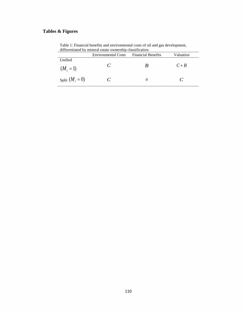
110
Tables & Figures
Table 1: Financial benefits and environmental costs of oil and gas development,
differentiated by mineral estate ownership classification
Environmental Costs Financial Benefits Valuation
Unified
)1( iM C B BC
Split )0( iM C 0 C
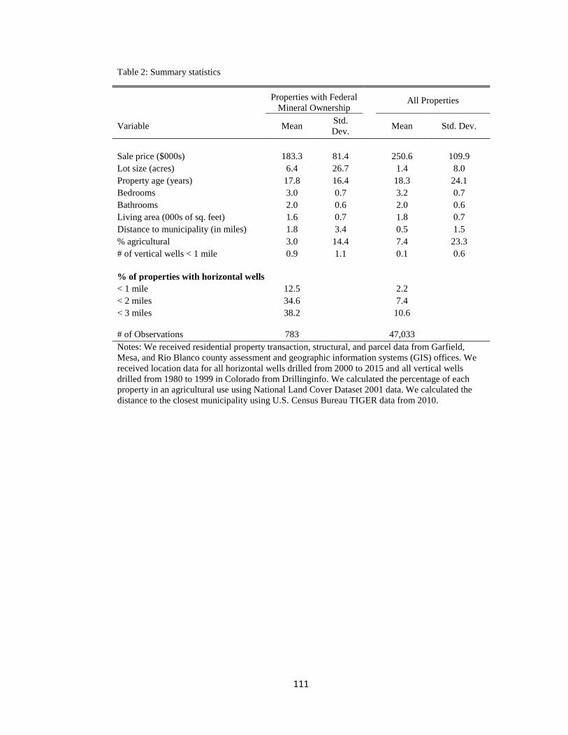
111
Table 2: Summary statistics
Properties with Federal
Mineral Ownership
All Properties
Variable Mean Std.
Dev.
Mean Std. Dev.
Sale price ($000s) 183.3 81.4 250.6 109.9
Lot size (acres) 6.4 26.7 1.4 8.0
Property age (years) 17.8 16.4 18.3 24.1
Bedrooms 3.0 0.7 3.2 0.7
Bathrooms 2.0 0.6 2.0 0.6
Living area (000s of sq. feet) 1.6 0.7 1.8 0.7
Distance to municipality (in miles) 1.8 3.4 0.5 1.5
% agricultural 3.0 14.4 7.4 23.3
# of vertical wells < 1 mile 0.9 1.1 0.1 0.6
% of properties with horizontal wells
< 1 mile 12.5 2.2
< 2 miles 34.6 7.4
< 3 miles 38.2 10.6
# of Observations 783 47,033
Notes: We received residential property transaction, structural, and parcel data from Garfield,
Mesa, and Rio Blanco county assessment and geographic information systems (GIS) offices. We
received location data for all horizontal wells drilled from 2000 to 2015 and all vertical wells
drilled from 1980 to 1999 in Colorado from Drillinginfo. We calculated the percentage of each
property in an agricultural use using National Land Cover Dataset 2001 data. We calculated the
distance to the closest municipality using U.S. Census Bureau TIGER data from 2010.
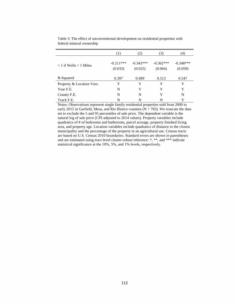
112
Table 3: The effect of unconventional development on residential properties with
federal mineral ownership
(1) (2) (3) (4)
= 1 if Wells < 1 Miles -0.211*** -0.343*** -0.362*** -0.348***
(0.033) (0.025) (0.064) (0.059)
R-Squared 0.397 0.499 0.513 0.547
Property & Location Vars. Y Y Y Y
Year F.E. N Y Y Y
County F.E. N N Y N
Track F.E. N N N Y
Notes: Observations represent single family residential properties sold from 2000 to
early 2015 in Garfield, Mesa, and Rio Blanco counties (N = 783). We truncate the data
set to exclude the 5 and 95 percentiles of sale price. The dependent variable is the
natural log of sale price (CPI-adjusted to 2014 values). Property variables include
quadratics of # of bedrooms and bathrooms, parcel acreage, property finished living
area, and property age. Location variables include quadratics of distance to the closest
municipality and the percentage of the property in an agricultural use. Census tracts
are based on U.S. Census 2010 boundaries. Standard errors are shown in parentheses
and are estimated using tract-level cluster-robust inference: *, **, and *** indicate
statistical significance at the 10%, 5%, and 1% levels, respectively.
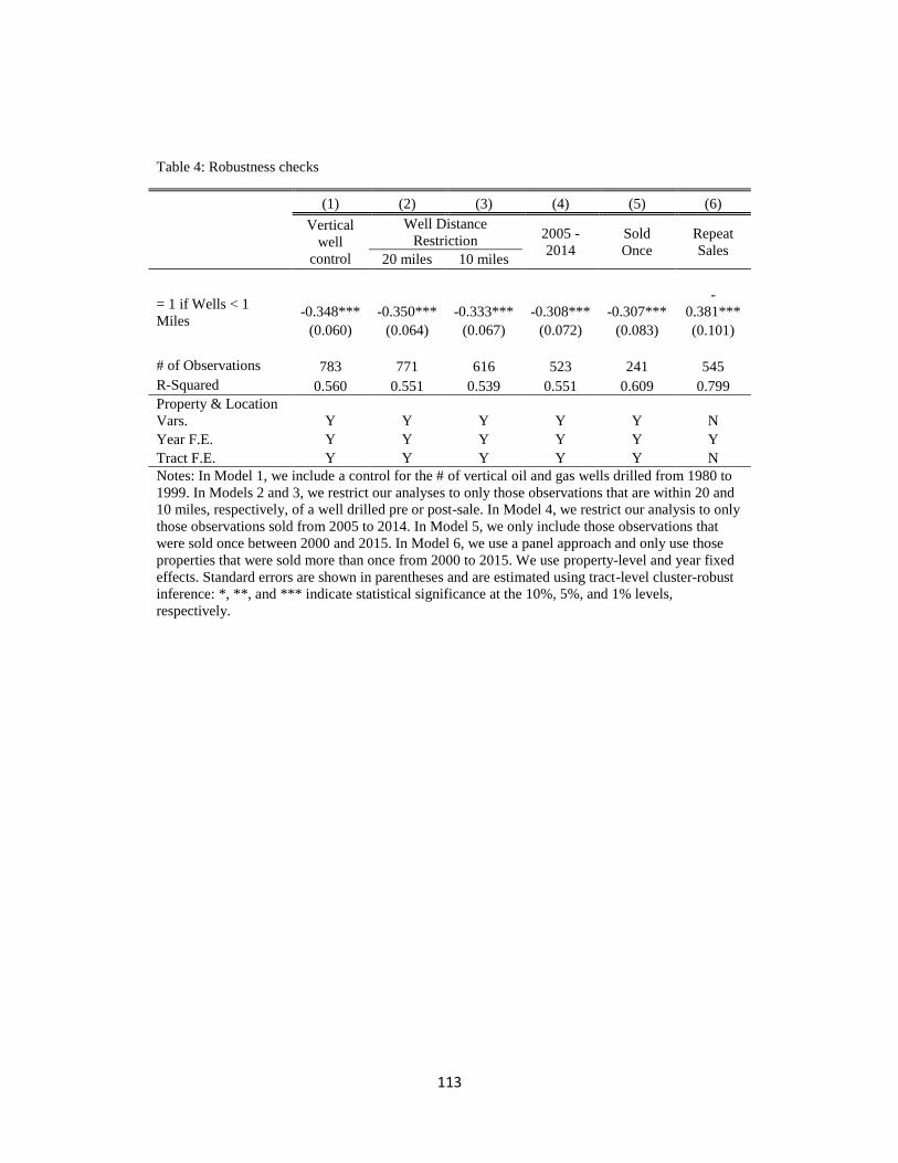
113
Table 4: Robustness checks
(1) (2) (3) (4) (5) (6)
Vertical
well
control
Well Distance
Restriction 2005 -
2014
Sold
Once
Repeat
Sales 20 miles 10 miles
= 1 if Wells < 1
Miles -0.348*** -0.350*** -0.333*** -0.308*** -0.307***
-
0.381***
(0.060) (0.064) (0.067) (0.072) (0.083) (0.101)
# of Observations 783 771 616 523 241 545
R-Squared 0.560 0.551 0.539 0.551 0.609 0.799
Property & Location
Vars. Y Y Y Y Y N
Year F.E. Y Y Y Y Y Y
Tract F.E. Y Y Y Y Y N
Notes: In Model 1, we include a control for the # of vertical oil and gas wells drilled from 1980 to
1999. In Models 2 and 3, we restrict our analyses to only those observations that are within 20 and
10 miles, respectively, of a well drilled pre or post-sale. In Model 4, we restrict our analysis to only
those observations sold from 2005 to 2014. In Model 5, we only include those observations that
were sold once between 2000 and 2015. In Model 6, we use a panel approach and only use those
properties that were sold more than once from 2000 to 2015. We use property-level and year fixed
effects. Standard errors are shown in parentheses and are estimated using tract-level cluster-robust
inference: *, **, and *** indicate statistical significance at the 10%, 5%, and 1% levels,
respectively.
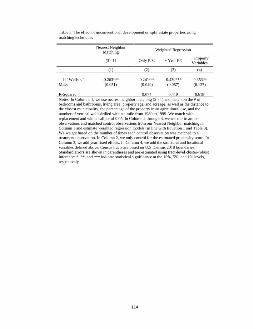
114
Table 5: The effect of unconventional development on split estate properties using
matching techniques
Nearest Neighbor
Matching
Weighted Regression
(3 - 1)
Only P.S. + Year FE
+ Property
Variables
(1) (2) (3) (4)
= 1 if Wells < 1
Miles
-0.263*** -0.241*** -0.439*** -0.353**
(0.051) (0.049) (0.057) (0.137)
R-Squared 0.074 0.410 0.618
Notes: In Columns 1, we use nearest neighbor matching (3 - 1) and match on the # of
bedrooms and bathrooms, living area, property age, and acreage, as well as the distance to
the closest municipality, the percentage of the property in an agricultural use, and the
number of vertical wells drilled within a mile from 1980 to 1999. We match with
replacement and with a caliper of 0.05. In Column 2 through 4, we use our treatment
observations and matched control observations from our Nearest Neighbor matching in
Column 1 and estimate weighted regression models (in line with Equation 1 and Table 3).
We weight based on the number of times each control observation was matched to a
treatment observation. In Column 2, we only control for the estimated propensity score. In
Column 3, we add year fixed effects. In Column 4, we add the structural and locational
variables defined above. Census tracts are based on U.S. Census 2010 boundaries.
Standard errors are shown in parentheses and are estimated using tract-level cluster-robust
inference: *, **, and *** indicate statistical significance at the 10%, 5%, and 1% levels,
respectively.
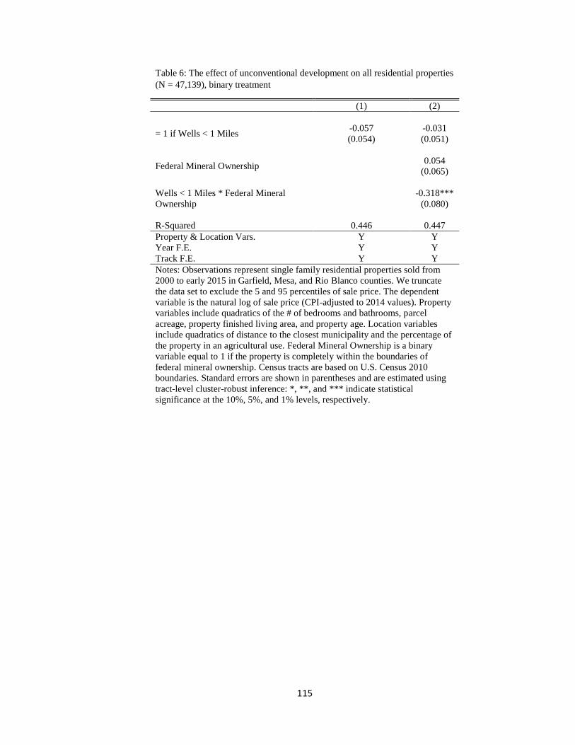
115
Table 6: The effect of unconventional development on all residential properties
(N = 47,139), binary treatment
(1) (2)
= 1 if Wells < 1 Miles -0.057 -0.031
(0.054) (0.051)
Federal Mineral Ownership 0.054
(0.065)
Wells < 1 Miles * Federal Mineral
Ownership
-0.318***
(0.080)
R-Squared 0.446 0.447
Property & Location Vars. Y Y
Year F.E. Y Y
Track F.E. Y Y
Notes: Observations represent single family residential properties sold from
2000 to early 2015 in Garfield, Mesa, and Rio Blanco counties. We truncate
the data set to exclude the 5 and 95 percentiles of sale price. The dependent
variable is the natural log of sale price (CPI-adjusted to 2014 values). Property
variables include quadratics of the # of bedrooms and bathrooms, parcel
acreage, property finished living area, and property age. Location variables
include quadratics of distance to the closest municipality and the percentage of
the property in an agricultural use. Federal Mineral Ownership is a binary
variable equal to 1 if the property is completely within the boundaries of
federal mineral ownership. Census tracts are based on U.S. Census 2010
boundaries. Standard errors are shown in parentheses and are estimated using
tract-level cluster-robust inference: *, **, and *** indicate statistical
significance at the 10%, 5%, and 1% levels, respectively.
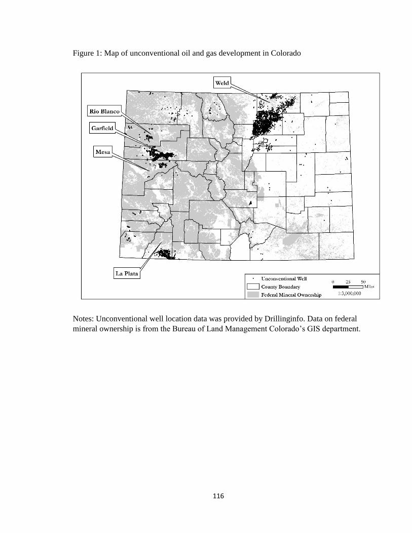
116
Figure 1: Map of unconventional oil and gas development in Colorado
Notes: Unconventional well location data was provided by Drillinginfo. Data on federal
mineral ownership is from the Bureau of Land Management Colorado’s GIS department.
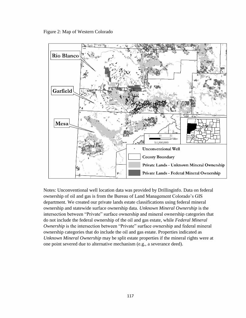
117
Figure 2: Map of Western Colorado
Notes: Unconventional well location data was provided by Drillinginfo. Data on federal
ownership of oil and gas is from the Bureau of Land Management Colorado’s GIS
department. We created our private lands estate classifications using federal mineral
ownership and statewide surface ownership data. Unknown Mineral Ownership is the
intersection between “Private” surface ownership and mineral ownership categories that
do not include the federal ownership of the oil and gas estate, while Federal Mineral
Ownership is the intersection between “Private” surface ownership and federal mineral
ownership categories that do include the oil and gas estate. Properties indicated as
Unknown Mineral Ownership may be split estate properties if the mineral rights were at
one point severed due to alternative mechanism (e.g., a severance deed).
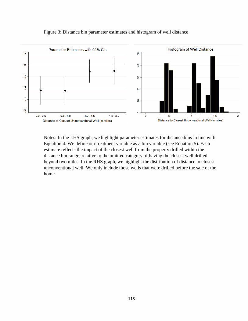
118
Figure 3: Distance bin parameter estimates and histogram of well distance
Notes: In the LHS graph, we highlight parameter estimates for distance bins in line with
Equation 4. We define our treatment variable as a bin variable (see Equation 5). Each
estimate reflects the impact of the closest well from the property drilled within the
distance bin range, relative to the omitted category of having the closest well drilled
beyond two miles. In the RHS graph, we highlight the distribution of distance to closest
unconventional well. We only include those wells that were drilled before the sale of the
home.
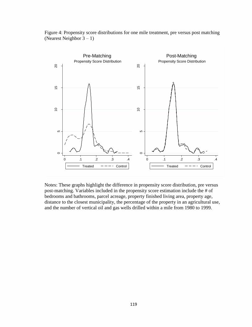
119
Figure 4: Propensity score distributions for one mile treatment, pre versus post matching
(Nearest Neighbor 3 – 1)
Notes: These graphs highlight the difference in propensity score distribution, pre versus
post-matching. Variables included in the propensity score estimation include the # of
bedrooms and bathrooms, parcel acreage, property finished living area, property age,
distance to the closest municipality, the percentage of the property in an agricultural use,
and the number of vertical oil and gas wells drilled within a mile from 1980 to 1999.
05
10
15
20
Kern
el D
en
sity
0 .1 .2 .3 .4
Treated Control
Propensity Score Distribution
Pre-Matching
05
10
15
20
0 .1 .2 .3 .4
Treated Control
Propensity Score Distribution
Post-Matching
120
Appendix
This Appendix provides information that is supplementary but not critical, to the
analyses that included in the main paper.
Table 1A includes a brief literature review of the literature on hedonic valuation
of unconventional oil and gas development. In this review, we focus on how mineral
rights ownership was discussed in each of the papers, especially in respect to how it
influenced their valuation. We do not summarize the results contained within each of
studies. The literature is discussed in greater detail in the main paper and all References
made in the table are listed in the Works Cited.
Table 2A provides a more comprehensive list of our parameter estimates in our
main specifications from Table 3 in the main text. The signs on the variables generally
match our expectations. Property price increases in acreage and living area but with
diminishing returns. Older houses sell for a discount. Property price decreases in the
number of bedrooms and bathrooms. This is unexpected, but this is not a concern given
correlation between both variables and living area. We generally find that property price
decreases as one moves further away from municipalities, though at a diminishing rate.
This is somewhat expected given the amenities associated with living in or near towns.
In Table 3A, we define treatment as the number of wells drilled within 1 mile.
The structure of the table is similar to that of Table 3 in the main paper. We find
qualitatively similar results when using this alternative treatment definition. Each well
drilled within a mile is associated with a decrease in sale price of 2%.
At the advice of an informal reviewer, we estimate Equation 4 in levels instead of
logs in Table 4A. We again find qualitatively similar results. In our preferred
121
specification in Column 4, we estimate that having an unconventional well within a mile
of a property decreases sale price by $52,000. This is similar to an analogous estimate
using the mean sale price in our study area and our estimate from Table 3, Column 4.
In Table 5A, we test for the robustness of our results in Table 3 of the main paper
across a number of additional models. In Column 1, we include only those properties that
are within three miles of a well drilled from 1980 to 1999. This model tests whether or
not our treatment effect estimates are associated with differing levels of historical oil and
gas development. In Columns 2 and 3, we relax our definition of a split estate – those
properties with federal mineral ownership – to allow properties with 90% and 75%
coverage, respectively, within federal mineral ownership boundaries. In Columns 4 and
5, we use alternative well distance restrictions to our 20 and 10 mile distances used in
Columns 2 and 3 from our robustness table in the main text. In Column 6, we cut
observations below the 5% and above the 95% distribution in acreage. We do this to
avoid the influence of outlying observations based on property size. Lastly, in Column 7,
we include mobile homes while also controlling for them using a binary indicator.
Our results from our additional models suggest that our results are robust. Our
results are similar when we relax our definition of the split estate. Although these
definitions are still restrictive and are likely including observations with federal mineral
ownership, they suggest that we could increase our sample size and still obtain similar
results. Our results are also similar to our main results when we use alternative
restrictions based on distance to the closest well and when we cut outlying observations
by acreage.
122
In Table 6A, we provide a brief summary of pre and post-matching statistics from
Table 5 in the main text. Mean standardized differences in the matching covariates are
reduced. Also, the Pseudo-R² is reduced and the p-value of the likelihood ratio test of
joint significance of the matching covariates is significantly higher, post-matching. These
results suggest that there are no differences in observed characteristics between control
and treatment observations, post-matching.
In Table 7A, we use our full sample in line with Table 6 in the main text. Instead
of only including properties with federal mineral ownership, we now include properties
with unknown mineral ownership. However, we now define treatment as the number of
unconventional wells drilled within a mile of the property. In Column 1, we find that
each well within a mile is associated with a 0.3% decrease in property sale price. This
effect is not significant and is much smaller than the estimates found in Table 2A (1.7 to
2.0%). In Column 2, we differentiate the effect of well development by whether or not
the property is within federal mineral ownership boundaries. We find that the effect of
well development is much larger for those properties with federal mineral ownership (-
1.6%). For those properties with unknown mineral ownership, the effect is close to zero
and insignificant. These findings support those from Table 6 in the main text. Since those
properties with unknown mineral ownership are likely to include properties with unified
mineral rights, our treatment effect for these properties is likely to be a net effect of
financial benefits and external costs of development.
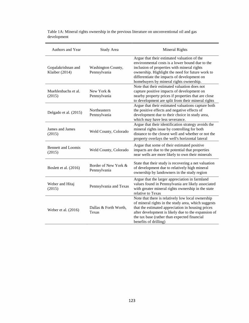
123
Table 1A: Mineral rights ownership in the previous literature on unconventional oil and gas
development
Authors and Year Study Area Mineral Rights
Gopalakrishnan and
Klaiber (2014)
Washington County,
Pennsylvania
Argue that their estimated valuation of the
environmental costs is a lower bound due to the
inclusion of properties with mineral rights
ownership. Highlight the need for future work to
differentiate the impacts of development on
homebuyers by mineral rights ownership.
Muehlenbachs et al.
(2015)
New York &
Pennsylvania
Note that their estimated valuation does not
capture positive impacts of development on
nearby property prices if properties that are close
to development are split from their mineral rights
Delgado et al. (2015) Northeastern
Pennsylvania
Argue that their estimated valuations capture both
the positive effects and negative effects of
development due to their choice in study area,
which may have less severance.
James and James
(2015) Weld County, Colorado
Argue that their identification strategy avoids the
mineral rights issue by controlling for both
distance to the closest well and whether or not the
property overlays the well's horizontal lateral
Bennett and Loomis
(2015) Weld County, Colorado
Argue that some of their estimated positive
impacts are due to the potential that properties
near wells are more likely to own their minerals
Boslett et al. (2016) Border of New York &
Pennsylvania
State that their study is recovering a net valuation
of development due to relatively high mineral
ownership by landowners in the study region
Weber and Hitaj
(2015) Pennsylvania and Texas
Argue that the larger appreciation in farmland
values found in Pennsylvania are likely associated
with greater mineral rights ownership in the state
relative to Texas
Weber et al. (2016) Dallas & Forth Worth,
Texas
Note that there is relatively low local ownership
of mineral rights in the study area, which suggests
that the estimated appreciation in housing prices
after development is likely due to the expansion of
the tax base (rather than expected financial
benefits of drilling)
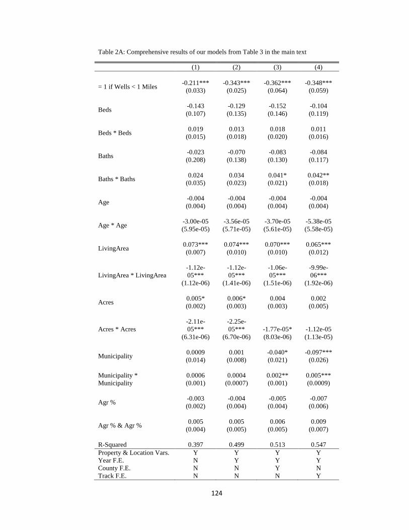
124
Table 2A: Comprehensive results of our models from Table 3 in the main text
(1) (2) (3) (4)
= 1 if Wells < 1 Miles -0.211*** -0.343*** -0.362*** -0.348***
(0.033) (0.025) (0.064) (0.059)
Beds -0.143 -0.129 -0.152 -0.104
(0.107) (0.135) (0.146) (0.119)
Beds * Beds 0.019 0.013 0.018 0.011
(0.015) (0.018) (0.020) (0.016)
Baths -0.023 -0.070 -0.083 -0.084
(0.208) (0.138) (0.130) (0.117)
Baths * Baths 0.024 0.034 0.041* 0.042**
(0.035) (0.023) (0.021) (0.018)
Age -0.004 -0.004 -0.004 -0.004
(0.004) (0.004) (0.004) (0.004)
Age * Age -3.00e-05 -3.56e-05 -3.70e-05 -5.38e-05
(5.95e-05) (5.71e-05) (5.61e-05) (5.58e-05)
LivingArea 0.073*** 0.074*** 0.070*** 0.065***
(0.007) (0.010) (0.010) (0.012)
LivingArea * LivingArea
-1.12e-
05***
-1.12e-
05***
-1.06e-
05***
-9.99e-
06***
(1.12e-06) (1.41e-06) (1.51e-06) (1.92e-06)
Acres 0.005* 0.006* 0.004 0.002
(0.002) (0.003) (0.003) (0.005)
Acres * Acres
-2.11e-
05***
-2.25e-
05*** -1.77e-05* -1.12e-05
(6.31e-06) (6.70e-06) (8.03e-06) (1.13e-05)
Municipality 0.0009 0.001 -0.040* -0.097***
(0.014) (0.008) (0.021) (0.026)
Municipality *
Municipality
0.0006 0.0004 0.002** 0.005***
(0.001) (0.0007) (0.001) (0.0009)
Agr % -0.003 -0.004 -0.005 -0.007
(0.002) (0.004) (0.004) (0.006)
Agr % & Agr % 0.005 0.005 0.006 0.009
(0.004) (0.005) (0.005) (0.007)
R-Squared 0.397 0.499 0.513 0.547
Property & Location Vars. Y Y Y Y
Year F.E. N Y Y Y
County F.E. N N Y N
Track F.E. N N N Y

125
Notes: Notes: This table displays coefficient estimates from our control variables in our
models highlighted in Table 3. Beds is the number of bedrooms in the property's house.
Baths is the number of bathrooms in the property's house. LivingArea is the square
footage of finished area in the property (in 00s). Acres is the property's acreage. Age is
the property's age (years). Municipality is the distance to closest municipality (U.S.
Census Bureau 2010). Agr % is the percentage of the property in an agricultural use
(National Land Cover Dataset 2001).
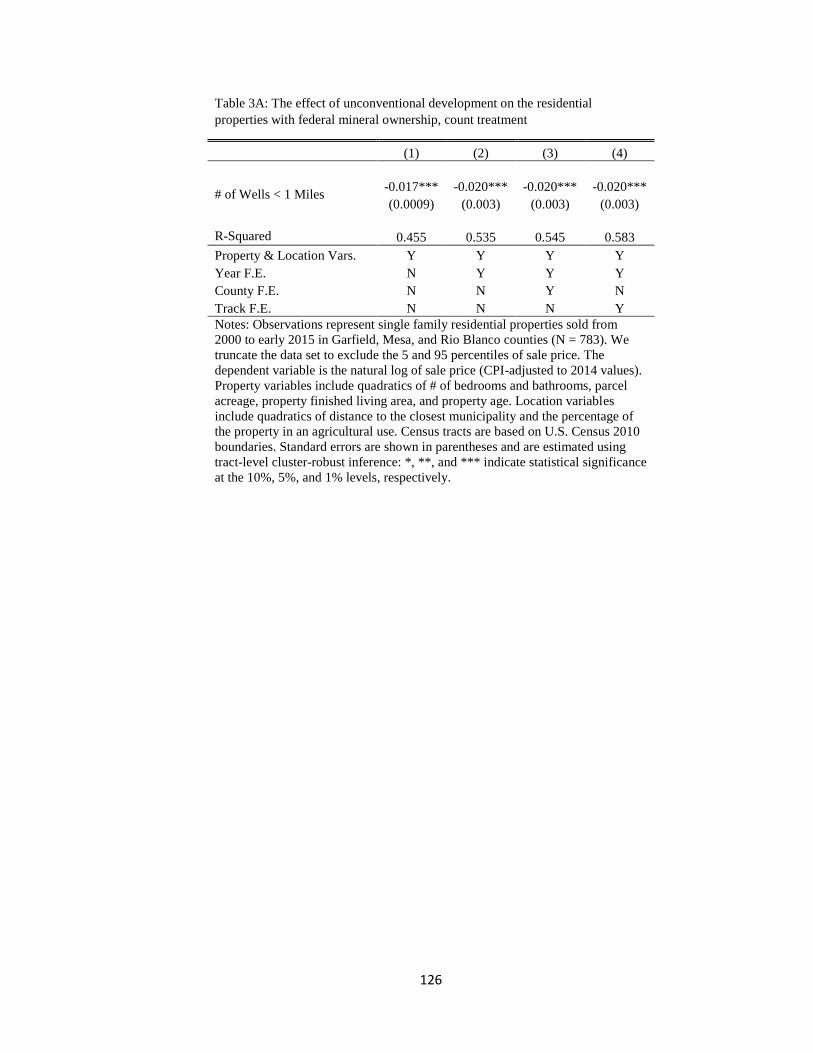
126
Table 3A: The effect of unconventional development on the residential
properties with federal mineral ownership, count treatment
(1) (2) (3) (4)
# of Wells < 1 Miles -0.017*** -0.020*** -0.020*** -0.020***
(0.0009) (0.003) (0.003) (0.003)
R-Squared 0.455 0.535 0.545 0.583
Property & Location Vars. Y Y Y Y
Year F.E. N Y Y Y
County F.E. N N Y N
Track F.E. N N N Y
Notes: Observations represent single family residential properties sold from
2000 to early 2015 in Garfield, Mesa, and Rio Blanco counties (N = 783). We
truncate the data set to exclude the 5 and 95 percentiles of sale price. The
dependent variable is the natural log of sale price (CPI-adjusted to 2014 values).
Property variables include quadratics of # of bedrooms and bathrooms, parcel
acreage, property finished living area, and property age. Location variables
include quadratics of distance to the closest municipality and the percentage of
the property in an agricultural use. Census tracts are based on U.S. Census 2010
boundaries. Standard errors are shown in parentheses and are estimated using
tract-level cluster-robust inference: *, **, and *** indicate statistical significance
at the 10%, 5%, and 1% levels, respectively.
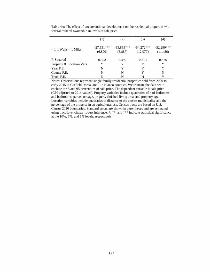
127
Table 4A: The effect of unconventional development on the residential properties with
federal mineral ownership in levels of sale price
(1) (2) (3) (4)
= 1 if Wells < 1 Miles -27,531*** -53,853*** -54,272*** -52,290***
(6,890) (5,887) (12,977) (11,486)
R-Squared 0.398 0.499 0.513 0.576
Property & Location Vars. Y Y Y Y
Year F.E. N Y Y Y
County F.E. N N Y N
Track F.E. N N N Y
Notes: Observations represent single family residential properties sold from 2000 to
early 2015 in Garfield, Mesa, and Rio Blanco counties. We truncate the data set to
exclude the 5 and 95 percentiles of sale price. The dependent variable is sale price
(CPI-adjusted to 2014 values). Property variables include quadratics of # of bedrooms
and bathrooms, parcel acreage, property finished living area, and property age.
Location variables include quadratics of distance to the closest municipality and the
percentage of the property in an agricultural use. Census tracts are based on U.S.
Census 2010 boundaries. Standard errors are shown in parentheses and are estimated
using tract-level cluster-robust inference: *, **, and *** indicate statistical significance
at the 10%, 5%, and 1% levels, respectively.
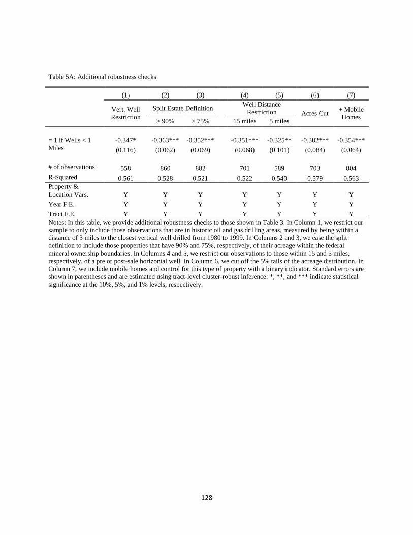
128
Table 5A: Additional robustness checks
(1) (2) (3) (4) (5) (6) (7)
Vert. Well
Restriction
Split Estate Definition Well Distance
Restriction Acres Cut + Mobile
Homes > 90% > 75% 15 miles 5 miles
= 1 if Wells < 1
Miles
-0.347* -0.363*** -0.352*** -0.351*** -0.325** -0.382*** -0.354***
(0.116) (0.062) (0.069) (0.068) (0.101) (0.084) (0.064)
# of observations 558 860 882 701 589 703 804
R-Squared 0.561 0.528 0.521 0.522 0.540 0.579 0.563
Property &
Location Vars. Y Y Y Y Y Y Y
Year F.E. Y Y Y Y Y Y Y
Tract F.E. Y Y Y Y Y Y Y
Notes: In this table, we provide additional robustness checks to those shown in Table 3. In Column 1, we restrict our
sample to only include those observations that are in historic oil and gas drilling areas, measured by being within a
distance of 3 miles to the closest vertical well drilled from 1980 to 1999. In Columns 2 and 3, we ease the split
definition to include those properties that have 90% and 75%, respectively, of their acreage within the federal
mineral ownership boundaries. In Columns 4 and 5, we restrict our observations to those within 15 and 5 miles,
respectively, of a pre or post-sale horizontal well. In Column 6, we cut off the 5% tails of the acreage distribution. In
Column 7, we include mobile homes and control for this type of property with a binary indicator. Standard errors are
shown in parentheses and are estimated using tract-level cluster-robust inference: *, **, and *** indicate statistical
significance at the 10%, 5%, and 1% levels, respectively.

129
Table 6A: Pre and post-matching statistics
Pre-Matching Post-Matching
Mean Normalized Bias 23.2 5.4
Pseudo R² 0.094 0.021
Likelihood Ratio Test P-Value < 0.001 0.756
Notes: We used Nearest Neighbor Matching (3 - 1) with replacement a 0.05 caliper. We
matched on the # of bedrooms and bathrooms, living area, property age, distance to
municipality, percentage of the property in an agricultural use, and the number of vertical wells
drilled within a mile from 1980 to 1999.
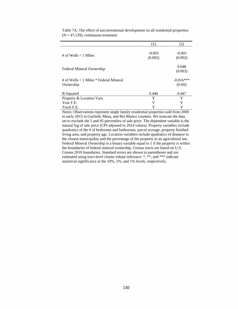
130
Table 7A: The effect of unconventional development on all residential properties
(N = 47,139), continuous treatment
(1) (2)
# of Wells < 1 Miles -0.003 -0.001
(0.002) (0.002)
Federal Mineral Ownership 0.048
(0.063)
# of Wells < 1 Miles * Federal Mineral
Ownership
-0.016***
(0.002
R-Squared 0.446 0.447
Property & Location Vars. Y Y
Year F.E. Y Y
Track F.E. Y Y
Notes: Observations represent single family residential properties sold from 2000
to early 2015 in Garfield, Mesa, and Rio Blanco counties. We truncate the data
set to exclude the 5 and 95 percentiles of sale price. The dependent variable is the
natural log of sale price (CPI-adjusted to 2014 values). Property variables include
quadratics of the # of bedrooms and bathrooms, parcel acreage, property finished
living area, and property age. Location variables include quadratics of distance to
the closest municipality and the percentage of the property in an agricultural use.
Federal Mineral Ownership is a binary variable equal to 1 if the property is within
the boundaries of federal mineral ownership. Census tracts are based on U.S.
Census 2010 boundaries. Standard errors are shown in parentheses and are
estimated using tract-level cluster-robust inference: *, **, and *** indicate
statistical significance at the 10%, 5%, and 1% levels, respectively.
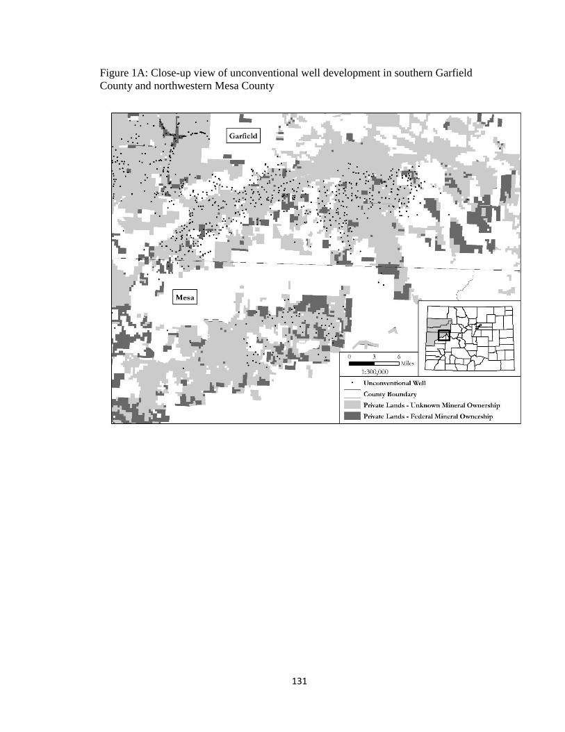
131
Figure 1A: Close-up view of unconventional well development in southern Garfield
County and northwestern Mesa County
132
Manuscript – 3
Prepared for submission to Resource and Energy Economics
A Bucket or a Sieve?
A Valuation of Views and Air Quality around Silica sand mining in Wisconsin
Andrew Boslett
Environmental and Natural Resource Economics, University of Rhode Island
133
Abstract
Silica sand mining has increased significantly since the beginning of the boom in
unconventional oil and gas development. This increase in mining has had economic,
environmental, and socio-economic impacts on local citizens. Yet, there has only been
limited work exploring these issues in the academic literature. In this study, I explore how
residential property buyers value the benefits and external costs of silica sand mining in
Wisconsin. To my knowledge, this is the first hedonic valuation of silica sand mining in
the academic literature. Evidence suggest that silica sand mining can decrease residential
property sale prices through viewshed and air quality impacts. These effects are
economically and statistically significant. I estimate stronger effects for those properties
that are subject to both viewshed impacts and air pollution from silica sand mining. I find
additional evidence that properties that are not subject to viewshed and air quality impacts
appreciate in value post-mining. This suggests that there is potential for post-mining
appreciation, perhaps associated with expectations of leasing-derived benefits from future
on-property mining or price premiums associated with property sales to mining companies.
Keywords: silica sand mining; hydraulic fracturing; hedonic valuation; viewshed; air
quality
134
1. Introduction
The demand for silica sand has increased measurably since the beginning of the
boom in unconventional oil and gas development. Silica sand is one of the key
ingredients in hydraulic fracturing, a process that has spurred significant oil and gas
production from previously inaccessible shale resources. This type of sand is the most
often-used proppant in hydraulic fracturing. A proppant is injected to maintain the
fractures created during hydraulic fracturing (Benson and Wilson 2015). Hydraulic
fracturing can require over 450 tons of proppant per well (King 2016). Although sand
mined in the Midwest United States has historically been used in a variety of
applications, most often in glass-making, the proportion of sand purchased by the oil and
gas industry has increased over time. It comes as no surprise that silica sand mining is
increasingly known as ‘frac’ sand mining.
Though the academic literature has explored many of the impacts of the
unconventional oil and gas boom, there has been considerably fewer studies on local
impacts associated with silica sand mining. These impacts can be both a blessing and a
curse. In terms of positive impacts, the increase in demand for silica sand from the oil and
gas industry has led to employment and income creation, a welcome boost for rural
communities that have not recovered from the great recession (Prengaman 2012). Sand
mining may also lead to growth in other sectors of the economy, including the rural rail
economy (Davies 2012a). Local landowners and farmers may also receive significant
signing bonuses and royalty payments from leasing their land to mining companies.
Others have sold their land outright to mining companies for prices above and beyond
assessed value (e.g., Davies 2012b; Lenker and Auch 2013; Dirr 2014; Mertens 2014).
135
Yet, these positive benefits are juxtaposed against environmental quality
concerns. Despite its name, ‘frac’ sand mining involves no hydraulic fracturing and is
instead extracted using surface mining techniques. This type of mining can take a
significant toll on the landscape by leveling hills and causing habitat fragmentation.
These mines can be very large; the average (maximum) size of permitted or operational
frac sand mines in Wisconsin is 341 (4000) acres (Wisconsin Department of Natural
Resources 2016). There are potential health concerns associated with increased local air
pollution and ambient silica dust (e.g., Pierce 2011). Sand mines also use a significant
amount of water and chemicals for sand processing (Wisconsin Department of Natural
Resources 2012; Minnesota Department of Health 2014). This may lead to local water
quality and quantity concerns for nearby farm owners and residents (Mundahl et al. 2014;
Verburg 2014). Many stakeholder groups have petitioned silica sand mining over these
environmental concerns (Pearson 2013) and some towns have passed short-term
moratoria on silica sand mining (Kennedy 2013).
The focus of this paper is on the residential property market in western
Wisconsin. As of 2016, there are over a hundred silica sand mines in the state, most of
which are located in counties along the Mississippi River. The growth in the industry has
been rapid over the last five years. In 2011 alone, the number of active sand mines
doubled in the state. From 2002 to 2013, total production of sand and gravel in Wisconsin
increased by around 1,100% (United States Geological Survey 2016). Figure 1 provides a
map of the current extent of silica sand mining in Wisconsin. Other states that have frac-
quality silica sand basins include Illinois, Iowa, Michigan, and Minnesota (Benson and
136
Wilson 2015), though as of 2014, Wisconsin produces over half of the United States’
total production of silica sand (Content 2015).
In this paper, I use hedonic pricing theory to value the local impacts of silica sand
mining in Wisconsin. This technique has a wide history of use in the economic literature
and has recently been applied to understand how people value unconventional oil and gas
development (e.g., Muehlenbachs et al. 2015). To my knowledge, this is the first
economic study to use hedonic valuation to understand how citizens value silica sand
mining’s impacts.
My approach relies on regression models that relate the level of local silica sand
mining to residential property sale prices. I first estimate a series of preliminary models
exploring how general proximity to silica sand mining has influenced residential property
sale prices from 2011 to 2016. I then explore the potential for heterogeneous impacts by
impact of mine. I focus on the capitalization of viewshed impacts and air quality impacts
associated with mining. These are two of the major environmental costs of sand mining. I
differentiate the effect of mining by whether or not it is in view of the residential
property. I hypothesize that having to view mining activity may negatively influence sale
price beyond the effect of mere proximity. My approaches are similar to those used in the
hedonic valuation of the impact of wind turbine views on housing prices (e.g.,
Heintzelman and Tuttle 2012; Gibbons 2015).41
41 This work builds on an extended literature incorporating property views into hedonic valuation models.
Much of this literature has focused on views of environmental amenities or natural land uses (see Bourassa
et al. 2004 for an extensive review). More recent work has focused on viewshed impacts associated with
energy infrastructure, including wind turbines and nuclear energy stations (e.g., Heintzelman and Tuttle
2012; Dickes et al. 2013; Lang et al. 2014; Gibbons 2015).
137
Following this analysis, I explore how air pollution and dust from mines influence
the sale price of residential properties. Given the rural character of my study area, I do
not have spatially-explicit air pollution data. Instead, I use an indicator of cardinal
direction away from each mine as a proxy for likelihood of air pollution associated with
mining. I argue that those properties on the eastward side of sand mines are more likely
to be impacted by dust and particulates from mining activity. An estimated differential
effect between properties in opposite directions away from the mine is likely to be
connected with greater air pollution effects on the eastward side of mines.
In my preliminary models, I find only weak evidence that silica sand mining has a
significant impact on residential property prices. When I differentiate by whether a
property is in-view or out-of-view of a mine, my results suggest that sand mining has a
negative impact on sale prices for those properties in-view of a mine. Each in-view frac
sand mine within two to four miles of the properties is associated with a 6 to 11%
decrease in property sale price. However, I do not find a significant impact of sand
mining that occurs within one mile of the property. Out-of-view sand mining generally
has positive effects on sale price, but these are not significant.
My hypothesis regarding air quality impacts is supported by my findings. Sand
mining from the west can have a negative impact on sale prices of downwind residential
properties. At the same time, I find significant evidence of appreciation for properties that
are upwind of mining activity. Each eastward sand mine within a mile of a property is
associated with an increase in property sale price of 12%. This effect decreases to around
10% for mines within one to two miles and to 3-4% for mines within two to four miles.
These effects are much stronger than the effects for corresponding westward mines.
138
Given the above results, I examine how silica sand mining influences residential
properties across indicators of both views of and the direction of mining activity.
Estimates suggest that silica sand mining from the west significantly reduces residential
property sale price, though the effect is considerably stronger for those properties that are
in view of a sand mine. I also find sale price appreciation for residential properties that
are out-of-view of eastward sand mining.
My results are suggestive of highly-localized positive capitalization of mining, as
well as significant negative capitalization of viewshed and air quality impacts for those
properties that are close but not adjacent to sand mining. Appreciation associated with
silica sand mining makes sense, as Wisconsin sand mines have expanded outward over
time42 and mining companies have been active in leasing or buying land outright for
mining (e.g., Davies 2012b; Dirr 2014). Appreciation may be linked to (1) property sales
to mining companies at prices above assessed values, or (2) expectations for this type of
sale price premium in the future (especially for those properties that are in close
proximity to mining activity but have not been sold to mining companies yet). It may also
be linked to property price compensation packages used by frac sand mine companies to
alleviate concerns from local residents regarding property price impacts. These packages
are used to compensate property owners for any losses in value, post-mining. According
to an unnamed county councilman in western Wisconsin, a sand mining company will
typically pay a premium over the listing price if a nearby residential property is unsold
six months after listing. It is currently unclear how often this type of transaction occurred
42 Based on aerial footprints of mines across time from Ted Auch, FracTracker Alliance.
139
in our data set. If it happened often, it may contribute to my findings of no change in
price or appreciation for certain properties.
At the same time, depreciation associated with silica sand mining appears to be
driven by both view and air quality changes. This is especially true for those properties
that are close but not adjacent to mining activity. Since I do not find any significant
evidence of environmental costs being capitalized within one mile, it seems as though the
benefits of mining are highly localized around mines but the costs are diffused outwards
from the mine to at least four miles away.
To my knowledge, this is the first economic study to explore the economic
impacts related to silica sand mining (concurrent with Kalinin et al. 2016). Although
Parker and Phaneuf (2013) provide a discussion of the potential impacts of silica sand
mining on property prices, their insights were based on price impacts associated with
other types of industrial activity. My results provide additional context of the mining-
driven changes that have occurred in rural areas of Wisconsin. I move beyond the
literature review and provide estimates of the impact of silica sand mining on nearby
property prices. Despite the recent slowdown in drilling, oil and gas development using
hydraulic fracturing is expected to continue in the future (United States Energy
Information Administration’s Annual Energy Outlook 2015). As a result, ‘frac’ sand
mining is likely to continue to be an issue in rural Wisconsin. Understanding how the
impacts of this type of sand mining are valued by local homeowners will be an important
topic into the foreseeable future. This study provides an important first step in
understanding how and why silica sand mining is capitalized into housing prices and
valued by homebuyers.
140
This paper is structured in the following manner. In Section 2, I provide
background on silica sand mining and its economic, environmental, and socio-cultural
implications. In Section 3, I discuss my study area of western Wisconsin and outline my
data. In Section 4, I highlight my methodological approach. In Section 5, I present my
empirical results and finish with some brief conclusions in Section 6.
2. Background
2.1. Silica sand mining in Wisconsin
Although sandstone basins are located in many areas of the United States, the
sandstone deposits in Wisconsin have characteristics that make it ideal in hydraulic
fracturing applications. This sand has a high silica content and mostly consists of quartz,
which is very hard (7.0 on the Mohs scale). As a result, it is able to resist pressure and
hold open fractures from hydraulic fracturing. The sand deposits in the region are also
generally close to the surface. This is in part a result of the fact that this general area of
Wisconsin avoided significant glaciation during the last ice age.43 This anomaly has made
it easier for companies to access and retrieve the sand through surface mining (Benson
and Wilson 2015).
2.2. Silica sand mining and its impacts
Academic research on the economic and socio-cultural impacts of silica sand
mining has been fairly limited. Deller and Schreiber (2012) explore the relationship
between general mining activity and various economic and socio-cultural variables,
though their methodology was unable to differentiate silica sand mining from other types
of mining. They also use county-level data at the national scale. Other economic studies
43 This is why this area of Wisconsin is known as the “Driftless Area” (Benson and Wilson 2015).
141
have been either non-academic or associated with stakeholder group funding. Power and
Power (2013) raise caution over high expectations of economic impact from silica sand
mining, but their suggestions are extrapolated from general mining activity across the
United States and rest of the world. Using IMPLAN and data from Illinois’ LaSalle
County, Harger (2015) estimates large direct and indirect employment and income effects
from local silica sand mining.44 In a review of literature related to the economic and
environmental impacts of industrial activity and mining, Parker and Phaneuf (2015)
suggest that silica sand mining may negatively impact property values and tourism in
Pepin County, Wisconsin. However, this conclusion was based on anecdote and insights
from the hedonic valuation literature of general industrial activity.
In the sociology literature, Pearson (2013) highlights community expectations
regarding the financial and employment benefits of silica sand mining versus the
environmental costs received by the general public in the vicinity of the mines. Although
some rural landowners may receive hundreds of thousands of dollars for selling their land
to mining companies, he generally describes the local community as opposed to silica
sand mining on environmental, public health, and socio-cultural grounds. In later work,
Pearson (2016) argues that the rapid pace and intensity of silica sand mining can reduce
residents’ sense of place and community.
A number of studies have explored the environmental impacts of silica sand
mining. Air pollution and increased silica dust in the local atmosphere is a prominent
concern in public media, though studies have found mixed results regarding the
magnitude of impact. Richards and Brozell (2015) were unable to detect differences in
44 As a note, this work was funded by the LaSalle County Mining Coalition and the Illinois Associate of Aggregate Producers.
142
upwind/downwind respiratory crystalline silica levels. However, Walters et al. (2015)
found PM2.5 levels above the Environmental Protection Agency’s annual standard.
Although each silica sand mine can use as much as 2.5 million gallons of water a day
(Wisconsin Department of Natural Resources 2012) and silica sand mining may change
groundwater aquifer recharge (Parsen and Gotkowitz 2013), there have been no studies
that evaluated pre and post-mining water quality in areas around silica sand mines.
However, in 2012, 20% of active mines and processing plants in Wisconsin were cited
for environmental violations (Prengaman 2013). Locke (2015) argues that this is an
increasing concern given that silica sand mines are often located in unzoned areas
without formal planning procedures.
2.3. Related hedonic valuation literature
There is a relatively limited literature on the hedonic valuation of mining activity
or its associated impacts. In early work, Hitzhusen et al. (1997) use lakeside property
prices to estimate the economic cost of pollution associated with abandoned strip mines
in Ohio. Their results indicate that close proximity to abandoned mines reduces the sale
price of properties. In later work, Damigos (2006) describes a National Resource Damage
Assessments that used hedonic valuation to value environmental costs of the Eagle Mine
in Colorado. The mine reduced sale price by $25,000 for those properties within six
miles. Williamson et al. (2007) explore the property price impacts associated with acid
mine drainage-impaired streams in West Virginia. They observe impacts of -$4,800 for
those properties located within a quarter-mile of an impaired stream.
To my knowledge, there are no studies using hedonic valuation to infer how
residents value the impacts of silica sand mining. Although Parker and Phaneuf (2013)
143
discuss some of potential implications of mining on housing prices, their insights are
based on a survey of the related literature on other types of mining and industrial activity.
3. Data
3.1. Study Area
My study area is focused in thirteen counties in western Wisconsin (Figure 2).
These counties are primarily rural with some scattered larger cities and towns, including
Chippewa Falls, Eau Claire, La Crosse, Marshfield, and Sparta. All counties overlay
sandstone formations that are sources of ‘frac’ sand and have experienced recent mining.
There are 95 ‘frac’ sand mines within the counties (out of 101 in the entire state). Many
of these mines were permitted between 2011 and 2016. Only seven of the mines were
permitted for reclamation prior to the mid-2000s, which is generally agreed as the starting
point to the boom in unconventional oil and gas development (Bauer 2014). There is
some limited evidence that another sixteen mines were in place in 2004, based on aerial
imagery from the National Agriculture Imagery Program (NAIP). However, this evidence
is highly subjective, as it is difficult to differentiate mining and agriculture in aerial
imagery.
3.2. Data
I use real estate transfer data from the Wisconsin Department of Revenue. This
data set includes all residential property transfers that occurred in Wisconsin since the
beginning of 2011. I only include those properties where the buyer and seller have no
prior relationship and where the seller has not retained any rights associated with the
property (e.g., a life estate or conservation easement). I also exclude multi-family
properties. To avoid using non-fair market value property sales, I cut all property
144
transactions with sale prices less than $20,000. After these cuts, I have 33,843 property
transactions in my study area.
Although this data set contains all residential property transactions since 2011, it
includes only a limited amount of property information. It comprises no information on
the structural characteristics of the property beyond whether it is a mobile or multi-family
home. However, I did receive structural characteristic data for a limited number of
properties from Chippewa, Eau Claire, Jackson, Monroe, and Trempealeau. This
information was provided by some of the state’s regional Multiple Listing Services. A
limitation of this data is that only those observations that were listed through the Multiple
Listing Service were included in their databases. For each county in my data set, only 30
to 60% of my observations have matching MLS data. Thus, I incorporate this data only as
a robustness check for my main models.
Using each property’s unique parcel identification code, I supplement my data
from the DOR by creating a rich dataset of locational information. I calculate the distance
to the closest perennial stream from the National Hydrography Dataset. I also calculate
the distance to the closest railway line and interstate highway (from the U.S. Census
Bureau, circa 2010). I calculate each property’s average elevation using data from the
Natural Resource Conservation Service’s Data Gateway. I use land cover data from the
National Land Cover Dataset (NLCD) 2011 to calculate the average agricultural and
forest land cover in and around each parcel.45
45 The parcel data that I used was not amenable to calculating statistics within parcel boundaries due to
some overlapping parcel boundaries. Thus, I used focal statistics in ArcGIS and calculated local statistics
within 500 meters around each parcel’s centroid. For example, instead of calculating the percentage of each
parcel in an agricultural use, I calculated the percentage of land in an agricultural use within a 500m buffer
of each parcel’s centroid.
145
I received silica sand mining location data from the Wisconsin Department of
Natural Resources.46 This data set included 127 silica sand mining locations, including
mines, processing and drying plants, rail stations, and resin coating facilities. I only
consider those facilities classified as performing at least some mining activity (N = 101).
All other facilities are dropped from the analysis.
The data set provides coordinate location and production status for all silica sand
mines in the state. However, the data does not include any information on when the
mines were first permitted or excavated. Most permitting and regulation of sand mining
in Wisconsin is done at the local level (e.g., Schuessler 2015). Although sand mines must
abide by state air and water regulations, all reclamation permitting is done either by the
county or the township where the mine is located. In order to commence non-metallic
mining, each company must receive a reclamation permit (Haines 2012). I received
reclamation permitting dates for 93 frac sand mines in Wisconsin through
correspondence with local county and township officials in zoning and land information
departments.47 I use this as my proxy for before-after status of mining for each property
transaction. If a property is close to mining activity that was permitted for reclamation
before the time-of-sale, then the property is considered “treated” by silica sand mining. If
the mine was permitted for reclamation after the time-of-sale, then the property is
considered a “control” observation since silica sand mining was not occurring at the time-
46 Wisconsin’s Department of Natural Resources’ “Locations of industrial sand mines and processing plants
in Wisconsin”, Microsoft Excel spreadsheet. 47 There were eight frac sand mines from which I could not find associated reclamation permitting
information. These eight mines were prospective mines as of January of 2016 that had only just applied for
reclamation permitting.
146
of-sale. Thus, for all analyses in this study, properties that are “treated” with nearby sand
mining are those that were sold after a mine was first permitted for reclamation.
I calculated the distance to and direction from all frac sand mines within twenty
miles for all properties in my study area. I used this information to estimate the distance
to the closest silica sand mine and the number of silica sand mines within different
buffers of each property’s extent. Additionally, I used ArcGIS and digital elevation data
to outline the viewshed of each sand mine in my study area. I estimated the local
viewshed of each mine’s centroid. Unfortunately, I did not have surveyed mine
boundaries that would better capture the extent of mining. The implication of this is that
both my distance and viewshed estimates are likely conservative. Properties are likely
closer to mining activity than what would be suggested by my distance measure and there
are likely some properties that are incorrectly classified as being out of a mine’s
viewshed. Future work will exploit mine boundaries aerial-digitized by Auch (2016).
4. Methodology
4.1. The effect of silica sand mining on local property prices
In my analyses, I estimate hedonic valuation models to value the impacts of silica
sand mining as perceived by home buyers in western Wisconsin. This approach has a
long history of use in applied economics research (see Rosen (1974) for an early outline
of the model). The main idea underlying the approach is that the price of a heterogeneous
good is associated with its attributes and characteristics. The price of the good can then
be decomposed as a function of its characteristics. This approach is particularly useful in
eliciting how homebuyers value the impacts associated with neighborhood amenities and
disamenities.
147
My first models relate the sale price of a home to the number of silica sand mines
that are within a series of distance bins away from the property:
(1) isttsistististist XMineMineP '
21 ...)21()10()ln(
istP is the sale price of residential property i at time t in census tract s. istMine )10( and
istMine )21( are equal to the number of frac sand mines within 0 – 1 miles and 1 – 2
miles, respectively, of property i at the time of sale, t (see Figure 3 for examples of frac
sand mine buffers of one mile, two miles, and five miles). The β parameters reflect the
percentage change of each sand mine within the given spatial area on the natural log of
sale price. Although I only show counts for two rings, I also include a count of mines
within 2 – 4 miles in my main specifications.
I control for property and location characteristics in'
istX , as well as census tract
fixed effects, s , and year fixed effects,
t . These fixed effects help control for
unobservable factors that vary across space and time and may influence the likelihood of
local sand mining and residential property sale price. This approach relies on the
comparison of a group of properties with a nearby sale mine permitted or in operation
before the sale of the property versus (1) those properties without a nearby mine at any
time and (2) those properties with a nearby mine permitted only after the sale of the
property.
I infer a valuation of the impacts of silica sand mining using my β parameters. In
these models, I do not identify separate impacts so any valuation from these parameters is
net of the benefits and costs of nearby mining. Given the possibility of both positive and
148
negative impacts associated with silica sand mining, I have no prior expectation of the
signs of these parameters.
To test for the robustness of these results, I estimate the model with alternative
subsets of the data. I describe each robustness check in Section 5.
4.2. The effect of silica sand mining’s viewshed changes on local property prices
Next, I explore the possibility of heterogeneous impacts based on certain
characteristics of the spatial relationship of each property to silica sand mining. I first
estimate how changes in views associated with silica sand mining impact nearby
residential property prices. The landscape and land use fragmentation impacts of silica
sand mining may lead to greater property price impacts for those properties that are in
sight of a nearby sand mine, ceteris paribus.
I estimate the following regression model:
(2) isttsist
ististist
X
YXMineNonVisibleYXeVisibleMinP
'
21 )()()ln(.
This distance bin-based approach is similar to that used in Tables 2 and 3 except I now
differentiate these counts by whether the mines are in-view or out-of-view of the
property. istYXeVisibleMin )( and istYXMineNonVisible )( are equal to the number of
the in-view and out-of-view frac sand mines, respectively, within X and Y miles of
property i at the time of sale, t. The β parameters now reflect the percentage change of
each in-view or out-of-view sand mine within X to Y miles on the natural log of sale
price. Although I only show counts for one arbitrary X – Y mile ring, I include multiple
mine counts in my main regression models (i.e., 0 to 1 miles, 1 to 2 miles, and 2 to 4

149
miles). I control for property and location characteristics, census tract fixed effects, and
year fixed effects.
I have no prior expectation of the sign of either 1 or
2 due to the potential for
the environmental costs of silica sand mining to be offset by positive appreciation,
perhaps due to expectations of a future sale premium from a mining company. However,
I believe that these parameters may both be positive if the costs of mining are lower than
any perceived financial benefits. On the other hand, they may both be negative if its costs
are greater than its positive impacts. However, I hypothesize that 1 will be attenuated if
2 is positive or larger in absolute magnitude if 2 is negative as a result of negative
capitalization of viewshed changes due to silica sand mining.
For any given X – Y spatial area, I estimate the viewshed impact of silica sand
mining by subtracting 2 from
1 . This value is the difference in housing price between
those properties in sight of a frac sand mine versus those out of sight of a frac sand mine,
post-permitting. For now, I argue that the only difference between these properties is the
impact of the viewshed itself, though I relax this assumption in my discussion of later
results.
To test for the robustness of my viewshed results, I estimate various alternatives
of Equation 1. These models vary by different subsets of the data. I describe them in
Section 5.
As an additional source of robustness, I follow Gibbons (2015) and use a slightly
different approach to identification. My viewshed approach described above defines
treatment using a bin framework, where I differentiate the effect of in-view and out-of-
view silica sand mining across different spatial areas. I now use a strict r mile buffer
150
approach and limit my observations to only those within r miles of a mine at any time. I
again include counts of both visible and non-visible frac sand mines, permitted prior to
the sale of the property, within r miles.
(3) isttsistististist XMineNonVisibleeVisibleMinP '
21)ln(
where istesVisibleMin is the number of visible frac sand mines located within r miles and
istMinesNonVisible is the number of non-visible frac sand mines located within the same
distance for residential property i at time t in census tract s. 1 and
2 indicate the
impact of each visible and non-visible sand mine, respectively, within r miles on
residential property sale price. I estimate this model across alternative values of r,
including integers from 1 to 4 miles.
For each buffer, I estimate two versions of Equation 3. The first model restricts
the control group to only include those properties that are close to nearby mining that has
not been permitted at the time-of-sale. Thus, these are properties that are close to future
mining sites. By restricting my control observations to only those properties that are close
to pre or post-sale mining, I avoid the potential issue of unobserved variability in housing
and neighbor stock across my study area. I am more likely comparing observations in my
control and treatment groups that are similar in characteristics and have experienced the
same local economic and market trends.
The second version is more inclusive and does not use this restriction. This model
incorporates control observations within twenty miles of present or future silica sand
mining. This is the approach applied in the analyses in Tables 2 through 4. Our control
observations are those properties that are either (1) close to future mining sites, as in the
151
first version of Equation 3, or (2) those residential properties that are outside of r miles
but within twenty miles of a mine permitted before or after the time of sale.
4.4. Heterogeneity across cardinal direction
I then test for heterogeneity of impact by cardinal direction in order to get a first-
order approximation of the impact of frac sand mine-driven air pollution on sale price. I
use westerly and easterly cardinal direction away from the mine’s meridian as a proxy for
prevailing wind conditions. I hypothesize that wind blows more often to the east. Thus,
those properties with westward frac sand mines are at a greater risk of air dust and
pollution versus those with eastward frac sand mines.
I estimate a structurally similar model to Equation 2:
(4) isttsist
ististist
X
YXEastwardYXWestwardP
'
21 )()()ln(
istYXWestward )( is the number of westward frac sand mines located within X and Y
miles and istYXEastward )( is the number of eastward frac sand mines located within
the same distance for residential property i at time t in census tract s. For each given X –
Y spatial area,1 and
2 indicate the impact of each westward and eastward sand mine,
respectively, on residential property sale price.
I again have no prior expectations of the sign of 1 or
2 . However, I hypothesize
that 1 will be attenuated or more negative relative to
2 as a result of presumed higher
levels of ambient dust and pollution for properties with westward-situated mining
activity.
152
I use the difference between 1 and
2 as a first-order approximation of the
capitalization of local air quality impacts in housing prices. The primary assumptions in
this interpretation is that (1) air quality effects are felt predominately by those on the
eastward side of mines, and (2) the only difference between properties on either side of
the mine is the relative levels of air pollution and dust. However, a concern is that my
control group - those mines with eastward mines - are likely to incur air quality impacts,
as well. To the extent that my control group suffers from spillover effects associated with
air quality impacts, my estimate is an underestimation of the valuation of air quality
impacts of silica sand mining in housing prices.
4.4. Heterogeneity across both viewshed and cardinal direction
In my last series of models, I combine my indicators from Equations 1 and 3 and
allow the impact of viewshed to vary based on cardinal direction from the mine. I now
differentiate across two margins: (1) in-view or out-of-view of a mine, and (2) east or
west of a mine (Equation 5):
(5)
isttsist
istist
ististist
X
EastwardNonVisibletwardVisibleEas
WestwardNonVisibletwardVisibleWesP
'
43
21)ln(
Each variable is a separate count of frac sand mines within r miles of each potential
combination of visibility and direction. Parameter interpretations are similar to those
above. They represent the differential impacts of each type of mine, specified by
visibility and direction, on residential property sale price.
Comparisons in parameters from 1 through
4 allow a more thorough
exploration of the implications of air pollution and views of frac sand mines on prices for
153
residential properties near frac sand mines. Each combination of visibility and cardinal
direction is associated with a different combination of impact. I hypothesize that 1 will
be the most negative or, if all parameters are positive, strongly attenuated parameter, due
to the fact that these properties are subject to both the viewshed and air pollution impacts
of silica sand mining. I also hypothesize that 4 will be the most positive or, if all
parameters are negative, strongly attenuated parameter, due to the fact that these
properties do not face either the viewshed or the air pollution impacts of silica sand
mining. I have no prior expectation of the relative differences between 2 and
3 since I
do not know whether the air pollution impact (i.e.,2 ) or the viewshed impact (i.e.,
3 )
will be more strongly valued in housing prices.
As a final note, this analysis allows us to estimate which properties are most
impacted by the viewshed and air pollution impacts of silica sand mining. Although I can
approximate the valuation of viewshed impacts by differencing my 1 from
2 or 3
from 4 , there may be concerns that those properties that are in view and to the east of
silica sand mining are also more subject to air pollution costs than those out-of-view but
also to the east of silica sand mining. This may be the case if topography serves as a
source of deposition of dust for those out-of-view properties to the east of mining. In this
case, the difference of 1 and
2 may capture viewshed impacts and the increased
impact of air pollution based on viewshed.
With that concern acknowledged, however, I still believe that this is an important
analysis. By controlling for both viewshed and cardinal direction, I obtain a more
nuanced understanding of the differential impact of silica sand mining across spatial and
topographical characteristics.
154
5. Results
5.1. The effect of silica sand mining’s viewshed changes on local property prices
I estimate Model 1 with treatments across three different spatial areas: a 0 to 1
mile buffer, a 1 to 2 mile ring, and a 2 to 4 mile ring. I control for a quadratic function of
property acreage, quadratic functions of a series of locational variables, year fixed
effects, and census tract fixed effects. My locational variables include the proximities to
the closest interstate highway and railroad and the percentage of land in an agricultural
use within 500 meters of the parcel's centroid. I only use those observations above the 5th
percentile and below the 95th percentile to reduce the potential for outlying sale prices (~
$30,000 to $340,000).
Table 1 provides summary statistics for my main sample, as well as those
properties that are within four miles of a frac sand mine, pre-sale. Properties share
generally similar characteristics, though properties near silica sand mining are also closer
to the interstate highway system and railroad system. This makes sense given the
transportation needs of silica sand mining production and transportation.
My results in Table 2 suggest that nearby silica sand mining can have a significant
and negative impact on residential property prices, though this effect seems to only exist
for properties with mines located between two to four miles away. However, this effect is
not statistically-significant when including census tract fixed effects. Across all models, I
uncover no evidence that mining has an influence on price within two miles.
These results are somewhat surprising. The typical assumption in the literature is
that environmental impacts diminish with increasing distance away from the source. In
the mining context, one would expect attenuating effects of proximity to sand mining as
one moves further away from mining activity. However, I find some limited evidence of
155
a significant effect of mining beyond two miles, but no effect of sand mining within two
miles.
Since census tract fixed effects help control for unobserved differences in housing
price across the study area, Column 4 in Table 2 is the preferred model. The estimate of
this model suggests no significant effect of sand mining on nearby property prices. To
test for the robustness of this non-result, I estimate models of Equation 1 with alternative
subsets of the data. In Column 1, I relax our restriction on sale price to only exclude those
observations sold for less than $20,000. Columns 2 through 4 gradually restrict the
dataset to avoid potential unobserved differences in spatially-varying characteristics that
drive sale price. In Column 2, I only include observations from census tracts with sand
mining activity at least within two miles away from the tract’s borders. In Column 3, I
exclude all observations that are outside of ten miles from the nearest sand mine. In
Column 4, I only include observations from those counties from which we have structural
characteristic information from the state’s Multiple Listing Service databases. Lastly, I
only include those observations with structural characteristic information in Column 5. In
this model, I also control for quadratic functions of the number of bedrooms, number of
bathrooms, and living area of the property.
My results in Table 3 provide further support for results in Column 4 of Table 2. I
am unable to find any significant evidence that silica sand mining has a significant net
effect on sale price. Although I find slightly larger estimates of some of our treatment
effects, none of these differences are significant.
5.2. The effect of silica sand mining’s viewshed changes on local property prices
156
My results from Tables 2 and 3 suggest that sand mining has at most a limited
effect on the sale price of residential property prices. I now explore whether this finding
of only a limited relationship is masking potential heterogeneity of valuation outside of a
pure distance measure.
I first explore whether the impact of local silica sand mining is different for those
properties that are in-view versus out-of-view of mining activity. In Table 4, I estimate
four models of Equation 2. In each column, I control for property characteristics, year
fixed effects, and census tract effects. In Columns 1 and 2, I restrict my control
observations to be within 20 and 10 miles, respectively, of mining activity. In Column 3,
I only include observations from those census tracts with sand mining activity or are
within two miles of a sand mine. In Column 4, I only include those observations that have
structural characteristic information from the MLS. I use these various subsets due to the
fact that my study area is extensive, covering thirteen counties. There may be significant
heterogeneity across the region, especially between those areas with silica sand mining
and those without it.
My results in Table 4 suggest that silica sand mining can be negatively capitalized
into residential properties prices if it is in-view of the property. This is especially true if
the mines are located from 1 to 4 miles away from the property. I estimate that each in-
view frac sand mine from 1 to 2 miles and 2 to 4 miles is associated with 5-7 and 10-11%
decreases, respectively, in sale price. Most estimated effects in these two bins are
statistically significant.
However, I find no statistically-significant impacts within 1 mile of the property.
In fact, the magnitude of the effect of in-view silica sand mining seems to increase as one
157
moves further away from the property. This result is again surprising. One would expect
that the impact of views would generally be smaller for properties that are further away
from mining.
I find some limited evidence that out-of-view silica sand mining has a
statistically-significant effect on nearby residential property prices. However, my
estimates are only statistically significant for one subset of the data – only those
properties in census tracts with silica sand mining – and only within the 1 to 2 mile ring. I
find that effects of out-of-view mining attenuate with increasing distance away, which is
the opposite of the relationship between estimated effect and distance away for in-view
mining.
These results provide some insight as to why I find significant effects only
beyond a certain distance away of mining activity. I find positive but statistically
insignificant effects for properties within one mile of out-of-view silica sand mining. This
may be driven by highly-localized expectations of financial benefits associated with silica
sand mining. As one moves further away from mining, these expectations diminish, as
suggested by out-of-view effects attenuating with increasing distance.
Yet, at the same time, I find that the effect of in-view mining increases with
increasing distance. It is possible that those properties beyond a mile of a mine are not
likely to receive financial benefits from leasing land for mining or selling land to mining
companies. If this is the case, then these properties face viewshed impacts without a
strong likelihood of compensation. For those properties that are in closer proximity to
silica sand mining (i.e., within a mile), there may be a stronger likelihood of financial
benefits, which may compensate for some of the viewshed impacts. This explanation is
158
speculative, but does make sense given the estimated relationships between in-view and
out-of-view mining and distance away from mining activity.
As an additional form of robustness, I follow Gibbons (2015) in Table 5 and focus
exclusively on those properties that are close to sand mining activity, pre or post-sale. In
doing so, I differentiate those properties sold after mining occurs by visibility of the frac
sand mines. Thus, I compare properties in-view and out-of-view of silica sand mining
after it occurs versus properties sold in the same area, pre-mining. By focusing in such a
small area, I remove the potential for omitted variable bias associated with differences
between control areas without mining versus treatment areas with mining.
I estimate Equation 3 across four different buffers with radii of 1, 2, 3, and 4
miles. I include two models for each distance buffer: (1) a model that only includes a
count of the visible sand mines at the time-of-sale, and (2) a model that includes counts
of both visible and non-visible sand mines at the time-of-sale. I use the same control
variables and fixed effects and sale price distribution from Tables 2 and 4.
All of these models suggest that visible sand mines have a negative impact on the
sale price of nearby residential properties. My estimates are statistically-significant for
the three and four mile buffers. I estimate that each visible sand mine within three miles
is associated with a 6% decrease in sale price. This effect increases in magnitude to 7-
8% at four miles.
However, I do not obtain statistically-significant effects for the one and two mile
buffers. Estimates for these buffers are also smaller in magnitude than those found in the
larger buffers. Although this is surprising, it matches up with what I found in Tables 2
through 4. There are two main reasons why this may be happening. First, I have a very
159
limited sample in these regions very close to mining activity. When I relax my
econometric specification and only control for year and census tract fixed effects, I obtain
stronger estimates in the -12 to -7% range that are close to statistical significance at the
10% level. Second, the potential financial benefits of silica sand mining that accrue to
landowners may complicate any comparison between models across buffer sizes. In-view
properties within one mile of a mine may have greater expectations of potential financial
benefits from mining activity than those that are in-view of mines, but are further away.
Those that are relatively far away from mining may have viewshed impacts without the
potential for compensation.
5.3. Heterogeneity across cardinal direction
In Table 5, I estimate Equation 3 using the same spatial areas defined in Table 2
and 3. I follow the structure of Table 3 and use various subsets of the data in order to test
for robustness of the result across different spatial restrictions. Instead of differentiating
by view of mining activity, I now differentiate properties sold after mining occurs by the
cardinal direction away from the frac sand mines. I hypothesize that properties with
westward mines are more likely to be negatively impacts by air pollution impacts from
silica sand mining than those properties with eastward mines.
Within the 2 to 4 mile ring away from the property, I generally find that each
silica sand mine from the west is associated with a decrease in sale price on the order of 2
to 3%. However, I do not find significant effects for properties within two miles.
Importantly, close proximity to eastward frac sand mines is associated with an
increase in property sale price, relative to pre-mining properties. This effect is statistically
significant across all treatment areas. The effects attenuate with increasing distance away,
160
as expected. The impact of each eastward frac sand mine within a mile is on the order of
12-13%. For eastward frac sand mines located within 1 to 2 miles, the impact is on the
order of 10%. From 2 to 4 miles, the effect is around 3.5%.
Negative estimates associated with westward sand mining provide supportive
evidence of capitalization of air pollution and ambient dust impacts of silica sand mining.
At the same time, positive estimates for eastward sand mining is suggestive of the
capitalization of either (1) actual or expected property prices premiums from direct sales
of land to mining companies, or (2) expected payments from leasing land for silica sand
mining.
5.4. Heterogeneity across both viewshed and cardinal direction
In Sections 5.1 through 5.3, I observed that viewshed and air quality impacts
influence the sale price of residential properties in close proximity to silica sand mining. I
now differentiate the effect of mining by both viewshed and cardinal direction at the
same time by estimating Equation 4. Each viewshed/direction combination captures a
different combination of impacts: (1) westward, visible frac sand mines influence both air
quality and viewshed, (2) westward, non-visible frac sand mines influence only air
quality, (3) eastward, visible frac sand mines influence only viewshed, and (4) eastward,
non-visible frac sand mines are subject to neither viewshed nor persistent air quality
impacts.
Evidence from Table 7 largely supports earlier results. Properties subject to both
viewshed and air quality impacts decrease in value across all four buffer sizes, though the
effect is only statistically significant from two to four miles (8-10% for each frac sand
mine). There is no effect of westward, non-visible mines. Additionally, I find evidence
161
of appreciation for those properties that are not impacted by either environmental cost
(i.e., those properties with non-visible, eastward mines). This effect is statistically
significant across all models and attenuates from 20% at 1 mile to 6% at 4 miles. My
estimates are not statistically significant for eastward, visible sand mines. However, the
difference in estimates for in-view and out-of-view eastward mines is suggestive of there
being a strong viewshed impact on property prices.
In Table 8, I test for the robustness of my results for my four mile buffer estimates
across alternative subsets of the data. My results from Table 8 generally support my
results from Table 7. Parameter estimates across the models are similar to those found in
Column 4. Some estimates are larger than from the main sample, but not significantly so.
From these results, it appears as those the properties that are most impacted by silica sand
mining are those properties that are both in-view and east of the mines. This makes sense,
as they are most subject to the viewshed and air pollution impacts of silica sand mining.
6. Conclusions
Although these results are exploratory, they are meaningful as a first step in a
longer analysis of the local economic impacts of silica sand mining. Overall, I find
evidence of both appreciation and depreciation associated with nearby silica sand mining.
My results suggest that silica sand mining’s impacts on local views and air quality can be
a source of depreciation in home values. Properties with westward mines decrease in
value, post-mining, whether or not they have a view of the mine. In-view, westward
mines have a larger influence on sale price than those out-of-view, though I am unable to
find significant viewshed effects for eastward mines. This may be driven by the small
number of observations with viewable, eastward mines. This may be a cause of concern
162
in Tables 4 and 5, where I do not control for cardinal direction of mines. If only 10% of
properties are in view of a mine, I may be misattributing my effect to viewshed when it is
more an air quality impact. There also may be an additive effect of air pollution for
properties in view of a mine versus those without a view of a mine. Deposition of sand
and particulates from mining on trees and topography may lead to greater air quality
effects for properties with a clear line of sight to a sand mine. Results from Tables 7 and
8 seem to support this possibility.
Although many frac sand mines were permitted after the beginning of my
dataset’s timeline, I do not have a large group of pre-mining control observations near
future mining sites, nor do I have a rich set of structural property characteristics from
which I could use as controls in a propensity score matching analysis. This limits my
ability to estimate causal relationships between silica sand mining and residential
property prices. It also makes it difficult to fully understand the balance in property
characteristics between those properties treated with mining and those that are not treated
with mining. The same issue is evident in my comparisons of observations across
different directions and views of silica sand mining. However, it is encouraging that my
results are similar when I only use those observations with structural information data
from the state’s Multiple Listing Services.
With that said, these findings reveal an intuitive and consistent story. Silica sand
mining seems to influence homebuyers, especially through viewshed and air quality
impacts. These results support anecdotal evidence from local residents in Wisconsin, as
well as the insights from Parker and Phaneuf (2013), that silica sand mining has
environmental impacts that may manifest in housing price decreases. At the same time,
163
some of my results suggest the possibility of limited price appreciation. Although the
mechanism is not clear, this may be due to expectations regarding future leasing activity
or direct sales to mining companies for a large premium. Future work in this literature
should focus on addressing the above issues to provide stronger policy information for
decision-makers and stakeholders in Wisconsin and the surrounding region.
164
References
Auch, Ted. 2016. Silica sand mine expansion ArcGIS data. FracTracker Alliance.
Bauer, R. Andrew. 2014. The unconventional oil and gas boom. Econ Focus Paper,
Federal Reserve Bank of Richmond.
Benson, Mary Ellen, and Anna B. Wilson. 2015. Frac sand in the United States – A
geological and industry overview. Open-File Report 2015-1107, U.S. Geological Survey,
U.S. Department of the Interior.
Bourassa, Steven C., Martin Hoesli, and Jian Sun. 2004. What’s in a view? Environment
and Planning A 36: 1427-1450.
Content, Thomas. 2015. Wisconsin’s frac sand industry booms. Milwaukee-Wisconsin
Journal Sentinel, May 28.
Damigos, Dimitris. 2006. An overview of environmental valuation methods for the
mining industry. Journal of Cleaner Production 14 (3-4): 234-247.
Davies, Phil. 2012a. Frac sand mining spurs rural rail. Fed Gazette publication, Federal
Reserve Bank of Minneapolis.
Davies, Phil. 2012b. Sand surge: In Minnesota and Wisconsin, frac sand mining has lifted
local economies – and stirred opposition. Fed Gazette publication, Federal Reserve Bank
of Minneapolis.
Deller, Stephen, and Andrew Schreiber. 2012. Frac sand mining and community
economic development. Staff Paper No. 565, Department of Agricultural & Applied
Economics, University of Wisconsin-Madison.
Dickes, Lori, David Wyman, and Steve Springs. 2013. The power of energy: Effects of a
nuclear power station on land sale prices. Appraisal Journal 81 (1): 34-44.
Dirr, Allison. 2014. Frac sand mines credited for rising, dropping property values.
Wisconsin Center for Investigative Journalism, March 30.
Farm Service Agency. 2004. National Aerial Imagery Program (NAIP). Aerial imagery
for Wisconsin. United States Department of Agriculture.
Fink, Alexander, and Thomas Stratmann. 2015. U.S. housing prices and the Fukushima
nuclear accident. Journal of Economic Behavior & Organization 117: 309-326.
Gibbons, Stephen. 2015. Gone with the wind: Valuing the visual impacts of wind
turbines through house prices. Journal of Environmental Economics and Management
72: 177-196.
165
Haines, Anna. 2012. Planning and zoning for “frac sand” mining. Center for Land Use
Education. University of Wisconsin – Stevens Point.
Harger, Brian, 2015. Economic impact analysis: The LaSalle County mining industry.
Center for Government Studies at Northern Illinois University. Analysis prepared on
behalf of the LaSalle County Mining Coalition and the Illinois Associate of Aggregate
Producers.
Heintzelman, Martin D., and Carrie M. Tuttle. 2012. Values in the wind: A hedonic
analysis of wind power facilities. Land Economics 88 (3): 571-588.
Hitzhusen, Fred J., Lauren Friedman, Kythrie Silva, and Diane Hite. 1997. Hedonic price
and travel cost estimation of strip mine impacts on lake-based property and recreation
values. Working paper, Department of Agricultural Economics, Ohio State University.
Homer, Collin, Jon Dewitz, Limin Yang, Suming Jin, Patrick Danielson, George Xian,
John Coulston, Nathaniel Herold, James Wickham, and Kevin Megown. Completion of
the 2011 National Land Cover Database for the conterminous United States –
Representing a decade of land cover change information. Photogrammetric Engineering
and Remote Sensing 81 (5); 345-354.
Kalinin, Alexey, Dominic Parker, Corbett Grainger, and Daniel Phaneuf. 2016. What the
frac? Sand mining and transport-induced externalities. Presentation, Allied Social
Sciences Associations 2016 Annual Conference.
Kennedy, Tony. 2013. Wisconsin county board approves moratorium on frac sand mines.
Minneapolis Star Tribune, August 19.
King, Hobart. 2016. What is frac sand? Geology: Geoscience News and Information.
Lang, Corey, James J. Opaluch, and George Sfinarolakis. 2014. The windy city: Property
value impacts of wind turbines in an urban setting. Energy Economics 44: 413-421.
Lenker, Brook, and Ted Auch. 2013. Sifting through sand mining. Article, FracTracker
Alliance.
Locke, Christina. 2015. Frac sand mines are preferentially sited in unzoned rural areas.
PLoS ONE 10 (7): e0131386.
Mertens, Richard. 2014. Next fracking controversy: In the Midwest, a storm brews over
‘frac sand’. The Christian Science Monitor, March 9.
Minnesota Department of Health. 2014. Silica sand mining and public health. Site
Assessment and Consultation Unit.
166
Muehlenbachs, Lucija, Elisheba Spiller, and Chris Timmins. 2015. The housing market
impacts of shale gas development. The American Economic Review 105 (12): 3633-3659.
Mundahl, Neal, Bruno Borsari, Caitlin Meyer, Philip Wheeler, Natalie Siderius, and
Sheila Harmes. 2014. Sustainable management of water quality in southeastern
Minnesota, USA: History, citizen attitudes, and future implications. In Sustainable Water
Use and Management. Springer International Publishing.
Parker, Dominic, and Daniel Phaneuf. 2013. The potential impacts of frac sand transport
and mining on tourism and property values in Lake Pepin communities. Report.
Parsen, Michael J., and Madeline B. Gotkowitz. 2013. Managing Chippewa County’s
groundwater – today and tomorrow: Evaluating the impacts of industrial sand mines and
irrigated agriculture on the county’s water resources. Factsheet 07, Wisconsin Geological
and Natural History Survey.
Pearson, Thomas. 2013. Frac sand mining in Wisconsin: Understanding emerging
conflicts and community organizing. Culture, Agriculture, Food and Environment: The
Journal of Culture & Agriculture 35 (1): 30-40.
Pearson, Thomas. 2016. Frac sand mining and the disruption of place, landscape, and
community in Wisconsin. Human Organization 75 (1): 47-58.
Pierce, Crispin. 2011. Health risks of frac sand mining and processing. Poster
presentation, National Environmental Health Association Meeting.
Power, Thomas Michael, and Donovan S. Power. 2013. The economic benefits and costs
of frac-sand mining in West Central Wisconsin: Phase one of study – General economic
& community overview. Report prepared for Wisconsin Farmers Union, Wisconsin
Towns Association and the Institute for Agriculture and Trade Policy
Prengaman, Kate. 2012. Frac sand boom creates thousands of jobs. Wisconsin Center for
Investigative Journalism, August 19.
Prengaman, Kate. 2013. Frac sand industry faces DNR violations, warnings. Wisconsin
Center for Investigative Journalism, March 3.
Richards, John, and Todd Brozell. 2015. Assessment of community exposure to ambient
respirable crystalline silica near frac sand processing facilities. Atmosphere 6 (8); 960-
982.
Rosen, Sherwin. 1974. Hedonic prices and implicit markets: Product differentiation in
pure competition. Journal of Political Economy 82 (1); 34-55.
Schuessler, Ryan. 2015. Wisconsin locals fear dust from mines for fracking sand even as
boom wanes. Al Jazeera America, November 6.
167
United States Census Bureau. 2010. TIGER/Line Shapefiles.
United States Energy Information Administration. 2015. Annual Energy Outlook.
Department of Energy.
United States Geological Survey. 2016. Minerals Yearbook: Silica (Includes Industrial
Sand and Gravel, Quartz Crystal, and Tripoli and Special Silica). 2002 and 2013
editions.
Natural Resources Conservation Service. 2016. National Hydrography Dataset for
Wisconsin. United States Department of Agriculture, produced with United States
Geological Survey and the Environmental Protection Agency.
Verburg, Steven. 2014. Frac sand miners fined $60,000 for stormwater spill in creek.
Wisconsin State Journal, September 9.
Walters, Kristin, Jeron Jacobson, Zachary Kroening, and Crispin Pierce. 2015. PM 2.5
airborne particulates near frac sand operations. Journal of Environmental Health 78 (4):
8-12.
Williamson, James M., Hale W. Thurston, and Matthew T. Heberling. 2008. Valuing acid
mine drainage remediation in West Virginia: A hedonic modeling approach. The Annals
of Regional Science 42 (4): 987-999.
Wisconsin Department of Natural Resources. 2012. Silica sand mining in Wisconsin.
Informational document.
Wisconsin Department of Revenue. 2016. Real estate transfer data. Microsoft Excel
spreadsheets.
Wisconsin Department of Natural Resources. 2016. Locations of industrial sand mines
and processing plants in Wisconsin. Microsoft Excel spreadsheet.
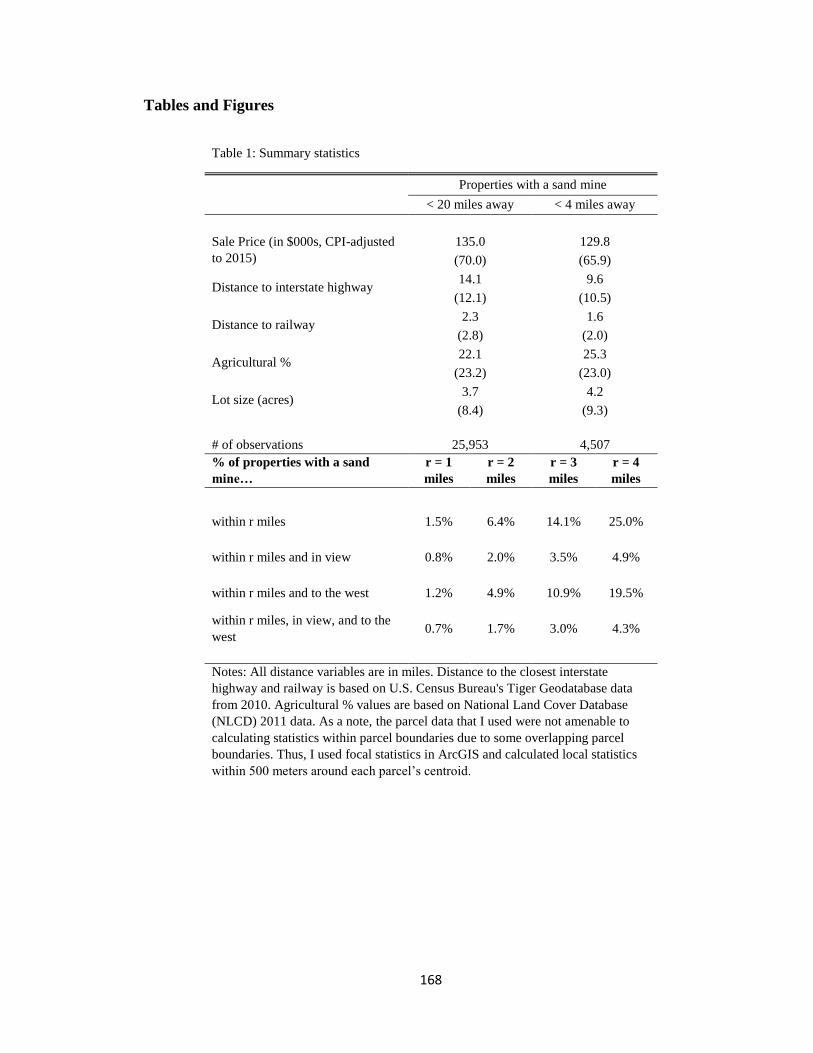
168
Tables and Figures
Table 1: Summary statistics
Properties with a sand mine
< 20 miles away < 4 miles away
Sale Price (in $000s, CPI-adjusted
to 2015)
135.0 129.8
(70.0) (65.9)
Distance to interstate highway 14.1 9.6
(12.1) (10.5)
Distance to railway 2.3 1.6
(2.8) (2.0)
Agricultural % 22.1 25.3
(23.2) (23.0)
Lot size (acres) 3.7 4.2
(8.4) (9.3)
# of observations 25,953 4,507
% of properties with a sand
mine…
r = 1
miles
r = 2
miles
r = 3
miles
r = 4
miles
within r miles 1.5% 6.4% 14.1% 25.0%
within r miles and in view 0.8% 2.0% 3.5% 4.9%
within r miles and to the west 1.2% 4.9% 10.9% 19.5%
within r miles, in view, and to the
west 0.7% 1.7% 3.0% 4.3%
Notes: All distance variables are in miles. Distance to the closest interstate
highway and railway is based on U.S. Census Bureau's Tiger Geodatabase data
from 2010. Agricultural % values are based on National Land Cover Database
(NLCD) 2011 data. As a note, the parcel data that I used were not amenable to
calculating statistics within parcel boundaries due to some overlapping parcel
boundaries. Thus, I used focal statistics in ArcGIS and calculated local statistics
within 500 meters around each parcel’s centroid.
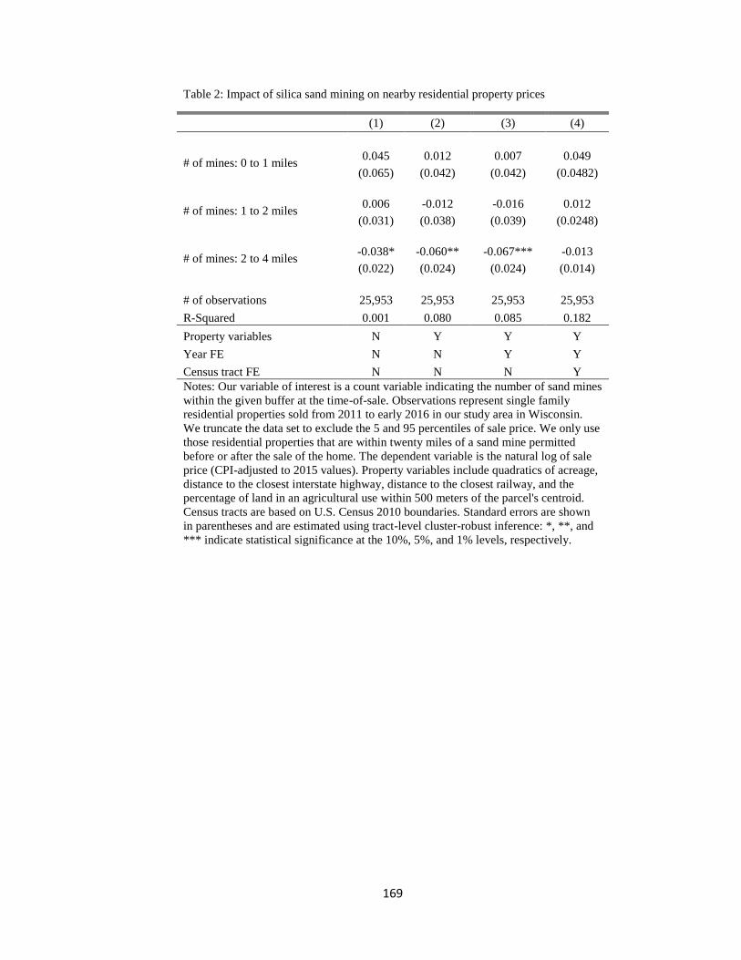
169
Table 2: Impact of silica sand mining on nearby residential property prices
(1) (2) (3) (4)
# of mines: 0 to 1 miles 0.045 0.012 0.007 0.049
(0.065) (0.042) (0.042) (0.0482)
# of mines: 1 to 2 miles 0.006 -0.012 -0.016 0.012
(0.031) (0.038) (0.039) (0.0248)
# of mines: 2 to 4 miles -0.038* -0.060** -0.067*** -0.013
(0.022) (0.024) (0.024) (0.014)
# of observations 25,953 25,953 25,953 25,953
R-Squared 0.001 0.080 0.085 0.182
Property variables N Y Y Y
Year FE N N Y Y
Census tract FE N N N Y
Notes: Our variable of interest is a count variable indicating the number of sand mines
within the given buffer at the time-of-sale. Observations represent single family
residential properties sold from 2011 to early 2016 in our study area in Wisconsin.
We truncate the data set to exclude the 5 and 95 percentiles of sale price. We only use
those residential properties that are within twenty miles of a sand mine permitted
before or after the sale of the home. The dependent variable is the natural log of sale
price (CPI-adjusted to 2015 values). Property variables include quadratics of acreage,
distance to the closest interstate highway, distance to the closest railway, and the
percentage of land in an agricultural use within 500 meters of the parcel's centroid.
Census tracts are based on U.S. Census 2010 boundaries. Standard errors are shown
in parentheses and are estimated using tract-level cluster-robust inference: *, **, and
*** indicate statistical significance at the 10%, 5%, and 1% levels, respectively.
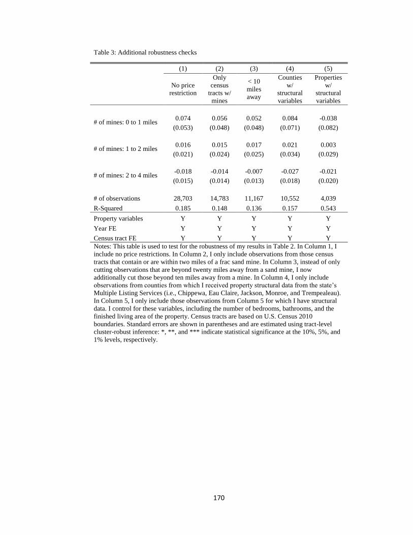
170
Table 3: Additional robustness checks
(1) (2) (3) (4) (5)
No price
restriction
Only
census
tracts w/
mines
< 10
miles
away
Counties
w/
structural
variables
Properties
w/
structural
variables
# of mines: 0 to 1 miles 0.074 0.056 0.052 0.084 -0.038
(0.053) (0.048) (0.048) (0.071) (0.082)
# of mines: 1 to 2 miles 0.016 0.015 0.017 0.021 0.003
(0.021) (0.024) (0.025) (0.034) (0.029)
# of mines: 2 to 4 miles -0.018 -0.014 -0.007 -0.027 -0.021
(0.015) (0.014) (0.013) (0.018) (0.020)
# of observations 28,703 14,783 11,167 10,552 4,039
R-Squared 0.185 0.148 0.136 0.157 0.543
Property variables Y Y Y Y Y
Year FE Y Y Y Y Y
Census tract FE Y Y Y Y Y
Notes: This table is used to test for the robustness of my results in Table 2. In Column 1, I
include no price restrictions. In Column 2, I only include observations from those census
tracts that contain or are within two miles of a frac sand mine. In Column 3, instead of only
cutting observations that are beyond twenty miles away from a sand mine, I now
additionally cut those beyond ten miles away from a mine. In Column 4, I only include
observations from counties from which I received property structural data from the state’s
Multiple Listing Services (i.e., Chippewa, Eau Claire, Jackson, Monroe, and Trempealeau).
In Column 5, I only include those observations from Column 5 for which I have structural
data. I control for these variables, including the number of bedrooms, bathrooms, and the
finished living area of the property. Census tracts are based on U.S. Census 2010
boundaries. Standard errors are shown in parentheses and are estimated using tract-level
cluster-robust inference: *, **, and *** indicate statistical significance at the 10%, 5%, and
1% levels, respectively.
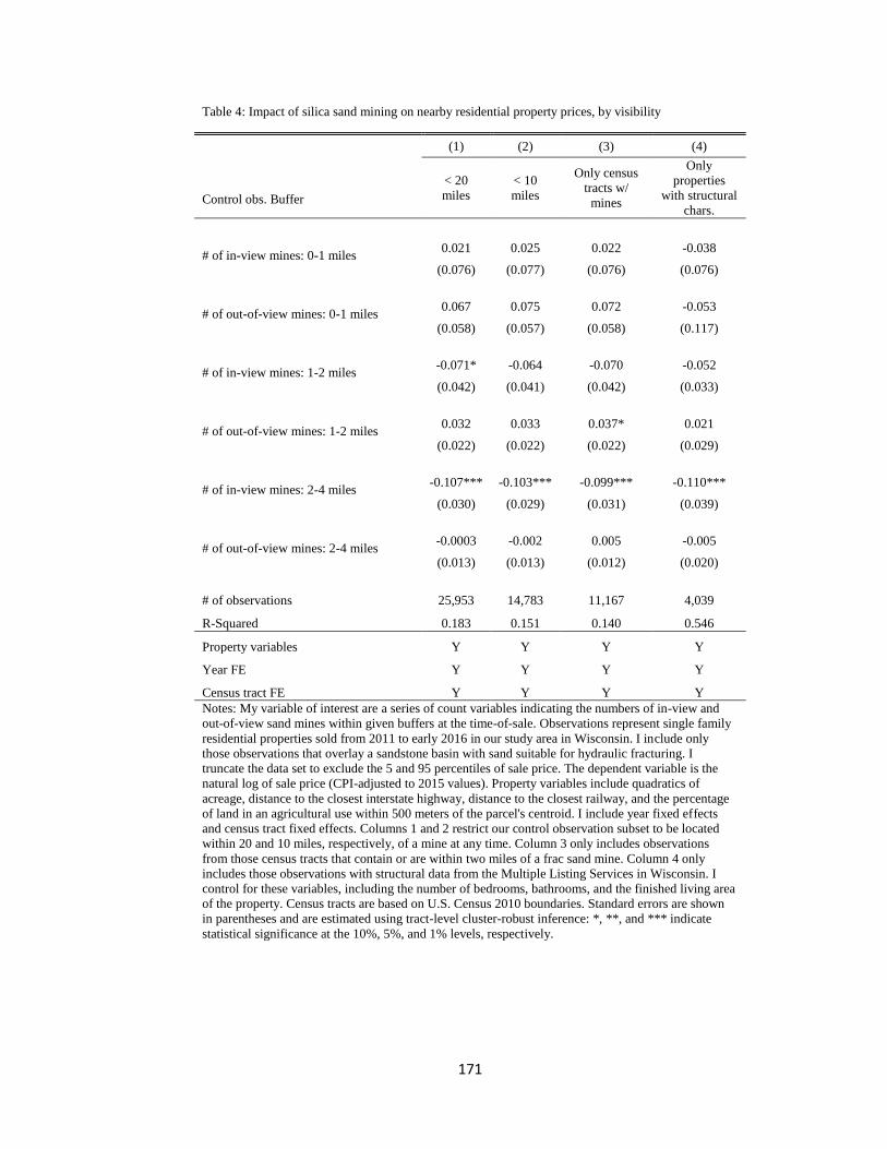
171
Table 4: Impact of silica sand mining on nearby residential property prices, by visibility
(1) (2) (3) (4)
< 20
miles
< 10
miles
Only census
tracts w/
mines
Only
properties
with structural
chars. Control obs. Buffer
# of in-view mines: 0-1 miles 0.021 0.025 0.022 -0.038
(0.076) (0.077) (0.076) (0.076)
# of out-of-view mines: 0-1 miles 0.067 0.075 0.072 -0.053
(0.058) (0.057) (0.058) (0.117)
# of in-view mines: 1-2 miles -0.071* -0.064 -0.070 -0.052
(0.042) (0.041) (0.042) (0.033)
# of out-of-view mines: 1-2 miles 0.032 0.033 0.037* 0.021
(0.022) (0.022) (0.022) (0.029)
# of in-view mines: 2-4 miles -0.107*** -0.103*** -0.099*** -0.110***
(0.030) (0.029) (0.031) (0.039)
# of out-of-view mines: 2-4 miles -0.0003 -0.002 0.005 -0.005
(0.013) (0.013) (0.012) (0.020)
# of observations 25,953 14,783 11,167 4,039
R-Squared 0.183 0.151 0.140 0.546
Property variables Y Y Y Y
Year FE Y Y Y Y
Census tract FE Y Y Y Y
Notes: My variable of interest are a series of count variables indicating the numbers of in-view and
out-of-view sand mines within given buffers at the time-of-sale. Observations represent single family
residential properties sold from 2011 to early 2016 in our study area in Wisconsin. I include only
those observations that overlay a sandstone basin with sand suitable for hydraulic fracturing. I
truncate the data set to exclude the 5 and 95 percentiles of sale price. The dependent variable is the
natural log of sale price (CPI-adjusted to 2015 values). Property variables include quadratics of
acreage, distance to the closest interstate highway, distance to the closest railway, and the percentage
of land in an agricultural use within 500 meters of the parcel's centroid. I include year fixed effects
and census tract fixed effects. Columns 1 and 2 restrict our control observation subset to be located
within 20 and 10 miles, respectively, of a mine at any time. Column 3 only includes observations
from those census tracts that contain or are within two miles of a frac sand mine. Column 4 only
includes those observations with structural data from the Multiple Listing Services in Wisconsin. I
control for these variables, including the number of bedrooms, bathrooms, and the finished living area
of the property. Census tracts are based on U.S. Census 2010 boundaries. Standard errors are shown
in parentheses and are estimated using tract-level cluster-robust inference: *, **, and *** indicate
statistical significance at the 10%, 5%, and 1% levels, respectively.
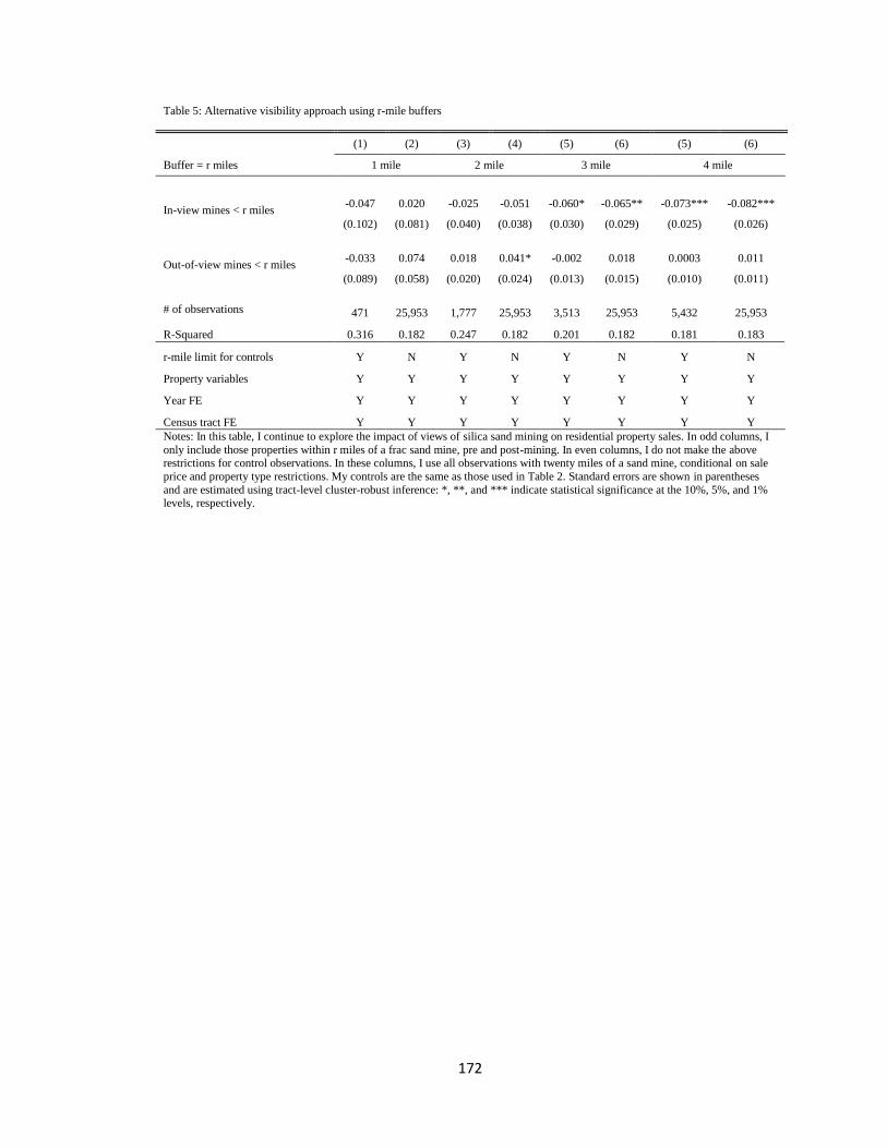
172
Table 5: Alternative visibility approach using r-mile buffers
(1) (2) (3) (4) (5) (6) (5) (6)
Buffer = r miles 1 mile 2 mile 3 mile 4 mile
In-view mines < r miles -0.047 0.020 -0.025 -0.051 -0.060* -0.065** -0.073*** -0.082***
(0.102) (0.081) (0.040) (0.038) (0.030) (0.029) (0.025) (0.026)
Out-of-view mines < r miles -0.033 0.074 0.018 0.041* -0.002 0.018 0.0003 0.011
(0.089) (0.058) (0.020) (0.024) (0.013) (0.015) (0.010) (0.011)
# of observations 471 25,953 1,777 25,953 3,513 25,953 5,432 25,953
R-Squared 0.316 0.182 0.247 0.182 0.201 0.182 0.181 0.183
r-mile limit for controls Y N Y N Y N Y N
Property variables Y Y Y Y Y Y Y Y
Year FE Y Y Y Y Y Y Y Y
Census tract FE Y Y Y Y Y Y Y Y
Notes: In this table, I continue to explore the impact of views of silica sand mining on residential property sales. In odd columns, I
only include those properties within r miles of a frac sand mine, pre and post-mining. In even columns, I do not make the above restrictions for control observations. In these columns, I use all observations with twenty miles of a sand mine, conditional on sale
price and property type restrictions. My controls are the same as those used in Table 2. Standard errors are shown in parentheses
and are estimated using tract-level cluster-robust inference: *, **, and *** indicate statistical significance at the 10%, 5%, and 1% levels, respectively.
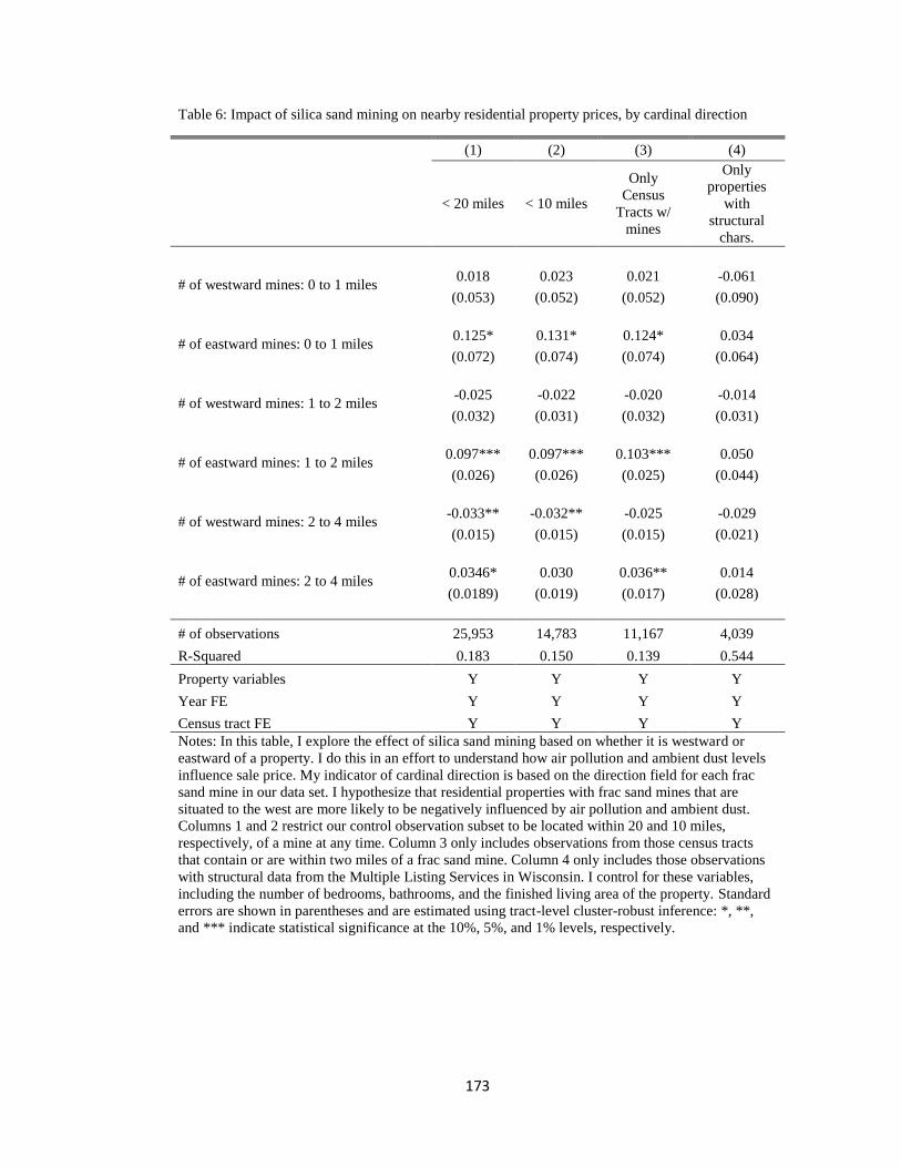
173
Table 6: Impact of silica sand mining on nearby residential property prices, by cardinal direction
(1) (2) (3) (4)
< 20 miles < 10 miles
Only
Census
Tracts w/
mines
Only
properties
with
structural
chars.
# of westward mines: 0 to 1 miles 0.018 0.023 0.021 -0.061
(0.053) (0.052) (0.052) (0.090)
# of eastward mines: 0 to 1 miles 0.125* 0.131* 0.124* 0.034
(0.072) (0.074) (0.074) (0.064)
# of westward mines: 1 to 2 miles -0.025 -0.022 -0.020 -0.014
(0.032) (0.031) (0.032) (0.031)
# of eastward mines: 1 to 2 miles 0.097*** 0.097*** 0.103*** 0.050
(0.026) (0.026) (0.025) (0.044)
# of westward mines: 2 to 4 miles -0.033** -0.032** -0.025 -0.029
(0.015) (0.015) (0.015) (0.021)
# of eastward mines: 2 to 4 miles 0.0346* 0.030 0.036** 0.014
(0.0189) (0.019) (0.017) (0.028)
# of observations 25,953 14,783 11,167 4,039
R-Squared 0.183 0.150 0.139 0.544
Property variables Y Y Y Y
Year FE Y Y Y Y
Census tract FE Y Y Y Y
Notes: In this table, I explore the effect of silica sand mining based on whether it is westward or
eastward of a property. I do this in an effort to understand how air pollution and ambient dust levels
influence sale price. My indicator of cardinal direction is based on the direction field for each frac
sand mine in our data set. I hypothesize that residential properties with frac sand mines that are
situated to the west are more likely to be negatively influenced by air pollution and ambient dust.
Columns 1 and 2 restrict our control observation subset to be located within 20 and 10 miles,
respectively, of a mine at any time. Column 3 only includes observations from those census tracts
that contain or are within two miles of a frac sand mine. Column 4 only includes those observations
with structural data from the Multiple Listing Services in Wisconsin. I control for these variables,
including the number of bedrooms, bathrooms, and the finished living area of the property. Standard
errors are shown in parentheses and are estimated using tract-level cluster-robust inference: *, **,
and *** indicate statistical significance at the 10%, 5%, and 1% levels, respectively.
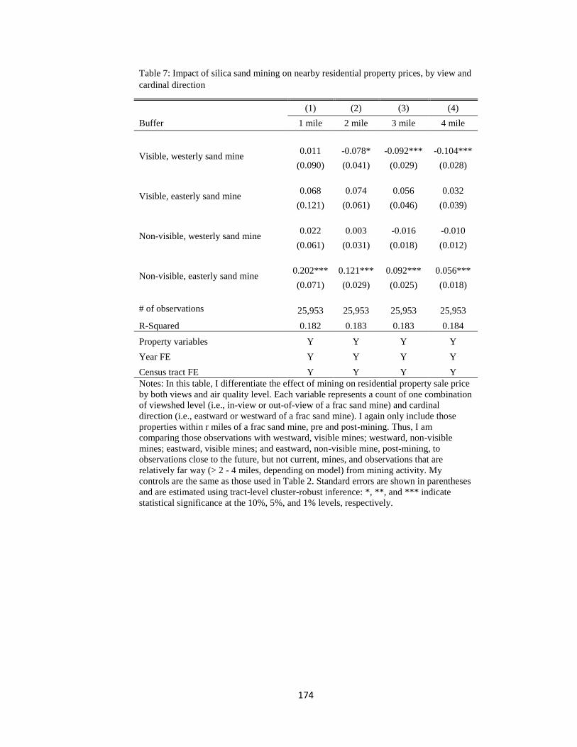
174
Table 7: Impact of silica sand mining on nearby residential property prices, by view and
cardinal direction
(1) (2) (3) (4)
Buffer 1 mile 2 mile 3 mile 4 mile
Visible, westerly sand mine 0.011 -0.078* -0.092*** -0.104***
(0.090) (0.041) (0.029) (0.028)
Visible, easterly sand mine 0.068 0.074 0.056 0.032
(0.121) (0.061) (0.046) (0.039)
Non-visible, westerly sand mine 0.022 0.003 -0.016 -0.010
(0.061) (0.031) (0.018) (0.012)
Non-visible, easterly sand mine 0.202*** 0.121*** 0.092*** 0.056***
(0.071) (0.029) (0.025) (0.018)
# of observations 25,953 25,953 25,953 25,953
R-Squared 0.182 0.183 0.183 0.184
Property variables Y Y Y Y
Year FE Y Y Y Y
Census tract FE Y Y Y Y
Notes: In this table, I differentiate the effect of mining on residential property sale price
by both views and air quality level. Each variable represents a count of one combination
of viewshed level (i.e., in-view or out-of-view of a frac sand mine) and cardinal
direction (i.e., eastward or westward of a frac sand mine). I again only include those
properties within r miles of a frac sand mine, pre and post-mining. Thus, I am
comparing those observations with westward, visible mines; westward, non-visible
mines; eastward, visible mines; and eastward, non-visible mine, post-mining, to
observations close to the future, but not current, mines, and observations that are
relatively far way (> 2 - 4 miles, depending on model) from mining activity. My
controls are the same as those used in Table 2. Standard errors are shown in parentheses
and are estimated using tract-level cluster-robust inference: *, **, and *** indicate
statistical significance at the 10%, 5%, and 1% levels, respectively.
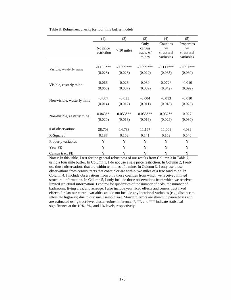
175
Table 8: Robustness checks for four mile buffer models
(1) (2) (3) (4) (5)
No price
restriction > 10 miles
Only
census
tracts w/
mines
Counties
w/
structural
variables
Properties
w/
structural
variables
Visible, westerly mine -0.105*** -0.099*** -0.099*** -0.111*** -0.091***
(0.028) (0.028) (0.029) (0.035) (0.030)
Visible, easterly mine 0.066 0.026 0.039 0.072* -0.010
(0.066) (0.037) (0.039) (0.042) (0.099)
Non-visible, westerly mine -0.007 -0.011 -0.004 -0.013 -0.010
(0.014) (0.012) (0.011) (0.018) (0.023)
Non-visible, easterly mine 0.043** 0.053*** 0.058*** 0.062** 0.027
(0.020) (0.018) (0.016) (0.029) (0.030)
# of observations 28,703 14,783 11,167 11,009 4,039
R-Squared 0.187 0.152 0.141 0.152 0.546
Property variables Y Y Y Y Y
Year FE Y Y Y Y Y
Census tract FE Y Y Y Y Y
Notes: In this table, I test for the general robustness of our results from Column 3 in Table 7,
using a four mile buffer. In Column 1, I do not use a sale price restriction. In Column 2, I only
use those observations that are within ten miles of a mine. In Column 3, I only use those
observations from census tracts that contain or are within two miles of a frac sand mine. In
Column 4, I include observations from only those counties from which we received limited
structural information. In Column 5, I only include those observations from which we received
limited structural information. I control for quadratics of the number of beds, the number of
bathrooms, living area, and acreage. I also include year fixed effects and census tract fixed
effects. I relax our control variables and do not include any locational variables (e.g., distance to
interstate highway) due to our small sample size. Standard errors are shown in parentheses and
are estimated using tract-level cluster-robust inference: *, **, and *** indicate statistical
significance at the 10%, 5%, and 1% levels, respectively.
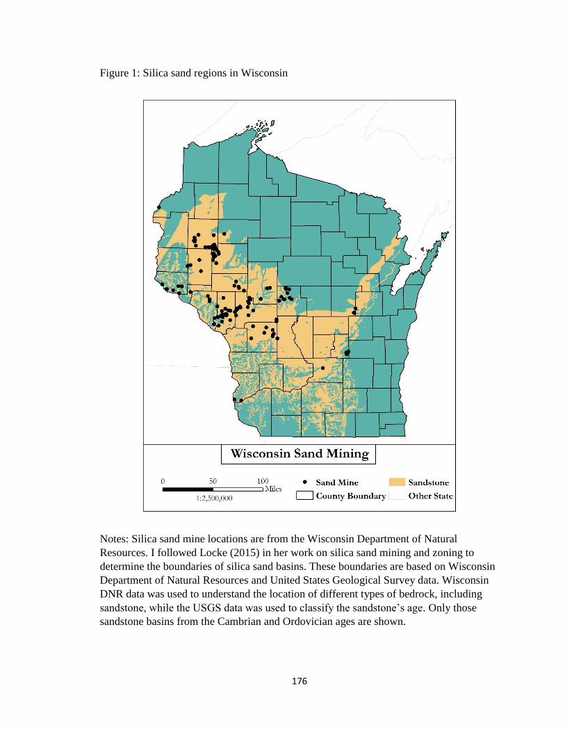
176
Figure 1: Silica sand regions in Wisconsin
Notes: Silica sand mine locations are from the Wisconsin Department of Natural
Resources. I followed Locke (2015) in her work on silica sand mining and zoning to
determine the boundaries of silica sand basins. These boundaries are based on Wisconsin
Department of Natural Resources and United States Geological Survey data. Wisconsin
DNR data was used to understand the location of different types of bedrock, including
sandstone, while the USGS data was used to classify the sandstone’s age. Only those
sandstone basins from the Cambrian and Ordovician ages are shown.
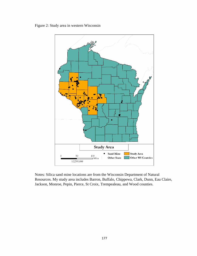
177
Figure 2: Study area in western Wisconsin
Notes: Silica sand mine locations are from the Wisconsin Department of Natural
Resources. My study area includes Barron, Buffalo, Chippewa, Clark, Dunn, Eau Claire,
Jackson, Monroe, Pepin, Pierce, St Croix, Trempealeau, and Wood counties.
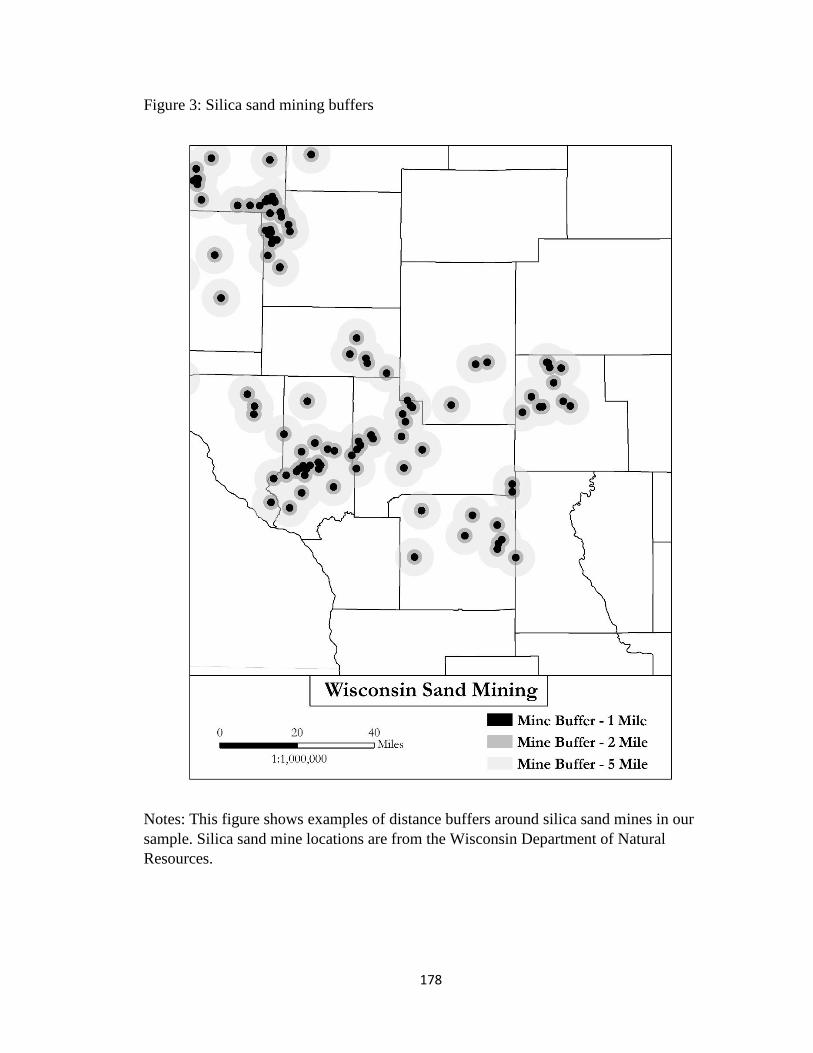
178
Figure 3: Silica sand mining buffers
Notes: This figure shows examples of distance buffers around silica sand mines in our
sample. Silica sand mine locations are from the Wisconsin Department of Natural
Resources.
179
Technical Appendix
Each manuscript of my dissertation relies heavily on hedonic valuation. This
technique was first outlined by Rosen (1974) and has a long history of use in the
economics literature. In this technical appendix, we describe the methodology’s
theoretical underpinnings and its key assumptions. We discuss the first and second stages
of hedonic valuation in turn.
First Stage of Hedonic Valuation
Hedonic valuation is based on the idea that a good’s price is related to levels of its
characteristics. This approach is only relevant to those classes of projects that are
differentiated in characteristics. This makes sense, as goods with homogeneous
characteristics would all sell at the same price. Two examples of goods that are
differentiated in terms of their characteristics include residential houses and automobiles.
All residential houses have beds and bathrooms, but the level of these assets varies across
houses. Some residential properties have two bedrooms; others have three bedrooms. On
the other hand, automobiles vary in size, miles per gallon, and interior options. Some
automobiles have leather interiors, while others have basic fabric interiors.
These and other characteristics of these types of goods influence sale price.
Residential property prices are generally higher for properties with more bedrooms;
automobile prices are higher for cars with a sunroof. These types of characteristic-price
relationships form the logic behind hedonic valuation. By exploring how sale prices
change in response to changes in characteristics, one can decompose how each
characteristic influences the good’s ultimate price at the margin.
180
How is a hedonic price function formed in a competitive market setting?
Following Rosen (1974) and Freeman (2003), consider a hypothetical housing market
where each house is decomposed into vectors of its characteristics:
(1) ),,( ENSh .
Characteristics of houses are included in three vectors: S includes structural
characteristics, such as the number of bedrooms, number of bathrooms, and acreage of
the property; N includes neighborhood characteristics, such as local school quality,
proximity to local grocery stores, and local crime levels; and E includes environmental
characteristics, such as the level of surrounding tree cover, air quality levels, and
proximity to local parks and greenspaces.
These characteristics are important in determining sale prices because they provide
utility to the consumer.
(2) ),,,( xENSU .
x is an index to represent all other utility-bearing goods consumed. Thus, consumers
essentially face a trade-off between characteristics associated with the house and what
they could buy in terms of all other goods. It is generally assumed that homebuyers have
perfect information regarding the level of these characteristics.
In this housing market, consumers are presented with a sufficiently large number
of options such that he or she can choose which house has the desired levels of
characteristics in terms of maximizing utility. Subject to their income, it is assumed that
consumers can locate anywhere in the market and that there are no transaction costs
associated with re-location.
181
It is also assumed that consumers cannot repackage goods through arbitrage. This
condition is important in that it ultimately leads to marginal prices that are non-linear.
This forbids consumers from buying two houses with different characteristic
combinations at a lower price than if they had only bought one house with the combined
characteristics from the two houses. As a result, the budget constraint for the consumers
is nonlinear: the marginal price of a characteristic is positive but decreases with
increasing levels of the characteristic.
Consumers are price-takers and observe price, )( ihp , which is a function of
property characteristics:
(3) ),,()( iiii ENSphp
In determining which house to buy, they consider each good’s bundle of characteristics
and their relationships to house price, conditional on their household budget, y:
(4) xZpy i )(
For simplification purposes, we combine iS ,
iN , and iE into a single vector of house
characteristic, iZ . Equation (4) states that what a consumer does not spend on a home is
spent on all other goods, x.
One can solve the utility-maximization using consumer optimization, which yields:
(5)
xU
ZU
Z
p i
i
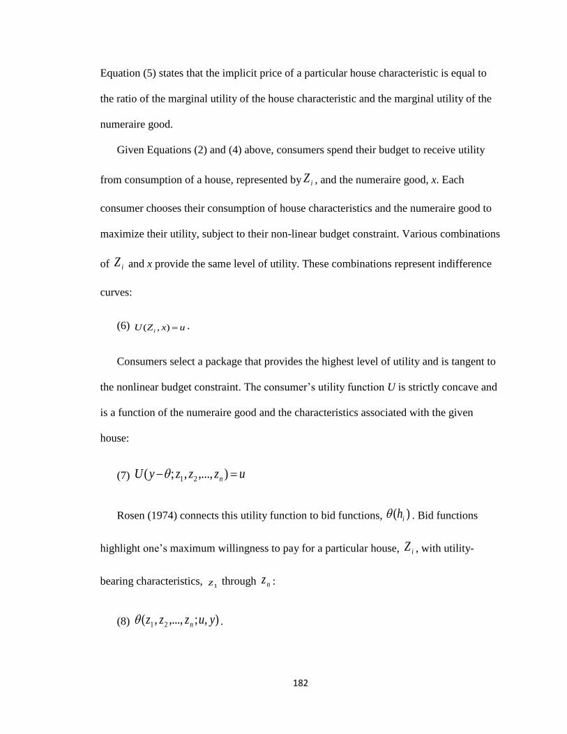
182
Equation (5) states that the implicit price of a particular house characteristic is equal to
the ratio of the marginal utility of the house characteristic and the marginal utility of the
numeraire good.
Given Equations (2) and (4) above, consumers spend their budget to receive utility
from consumption of a house, represented by iZ , and the numeraire good, x. Each
consumer chooses their consumption of house characteristics and the numeraire good to
maximize their utility, subject to their non-linear budget constraint. Various combinations
of iZ and x provide the same level of utility. These combinations represent indifference
curves:
(6) uxZU i ),( .
Consumers select a package that provides the highest level of utility and is tangent to
the nonlinear budget constraint. The consumer’s utility function U is strictly concave and
is a function of the numeraire good and the characteristics associated with the given
house:
(7) uzzzyU n ),...,,;( 21
Rosen (1974) connects this utility function to bid functions, )( ih . Bid functions
highlight one’s maximum willingness to pay for a particular house, iZ , with utility-
bearing characteristics, 1z through nz :
(8) ),;,...,,( 21 yuzzz n .
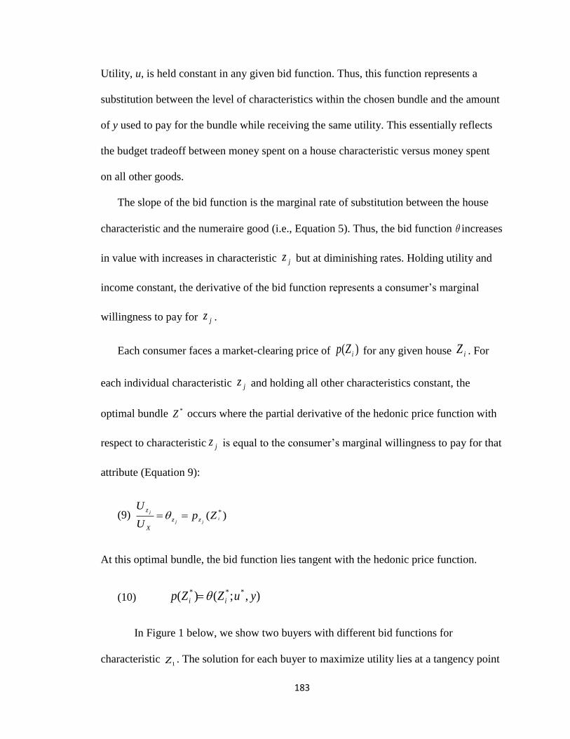
183
Utility, u, is held constant in any given bid function. Thus, this function represents a
substitution between the level of characteristics within the chosen bundle and the amount
of y used to pay for the bundle while receiving the same utility. This essentially reflects
the budget tradeoff between money spent on a house characteristic versus money spent
on all other goods.
The slope of the bid function is the marginal rate of substitution between the house
characteristic and the numeraire good (i.e., Equation 5). Thus, the bid function increases
in value with increases in characteristic jz but at diminishing rates. Holding utility and
income constant, the derivative of the bid function represents a consumer’s marginal
willingness to pay for jz .
Each consumer faces a market-clearing price of )( iZp for any given house iZ . For
each individual characteristic jz and holding all other characteristics constant, the
optimal bundle *Z occurs where the partial derivative of the hedonic price function with
respect to characteristic jz is equal to the consumer’s marginal willingness to pay for that
attribute (Equation 9):
(9) )( *i
jj
j
ZpU
Uzz
X
z
At this optimal bundle, the bid function lies tangent with the hedonic price function.
(10) ),;()( *** yuZZp ii
In Figure 1 below, we show two buyers with different bid functions for
characteristic 1Z . The solution for each buyer to maximize utility lies at a tangency point
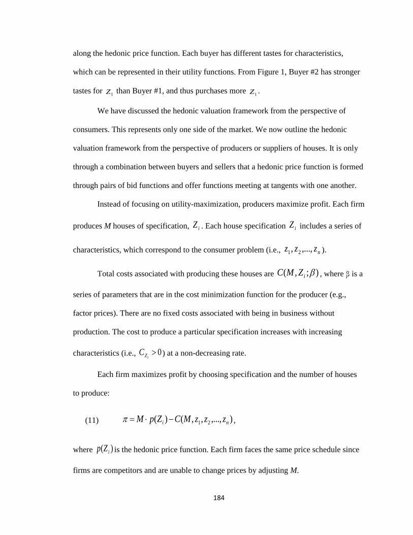
184
along the hedonic price function. Each buyer has different tastes for characteristics,
which can be represented in their utility functions. From Figure 1, Buyer #2 has stronger
tastes for 1Z than Buyer #1, and thus purchases more
1Z .
We have discussed the hedonic valuation framework from the perspective of
consumers. This represents only one side of the market. We now outline the hedonic
valuation framework from the perspective of producers or suppliers of houses. It is only
through a combination between buyers and sellers that a hedonic price function is formed
through pairs of bid functions and offer functions meeting at tangents with one another.
Instead of focusing on utility-maximization, producers maximize profit. Each firm
produces M houses of specification, iZ . Each house specification iZ includes a series of
characteristics, which correspond to the consumer problem (i.e., nzzz ,...,, 21 ).
Total costs associated with producing these houses are );,( iZMC , where β is a
series of parameters that are in the cost minimization function for the producer (e.g.,
factor prices). There are no fixed costs associated with being in business without
production. The cost to produce a particular specification increases with increasing
characteristics (i.e., 0iZC ) at a non-decreasing rate.
Each firm maximizes profit by choosing specification and the number of houses
to produce:
(11) ),...,,,()( 21 ni zzzMCZpM ,
where )( iZp is the hedonic price function. Each firm faces the same price schedule since
firms are competitors and are unable to change prices by adjusting M.
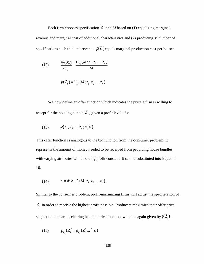
185
Each firm chooses specification iZ and M based on (1) equalizing marginal
revenue and marginal cost of additional characteristics and (2) producing M number of
specifications such that unit revenue )( iZp equals marginal production cost per house:
(12) M
zzzMC
z
Zp nz
j
i j),...,,;()( 21
),...,,;()( 21 nMi zzzMCZp
We now define an offer function which indicates the price a firm is willing to
accept for the housing bundle, iZ , given a profit level of π.
(13) ),;,...,,( 21 nzzz
This offer function is analogous to the bid function from the consumer problem. It
represents the amount of money needed to be received from providing house bundles
with varying attributes while holding profit constant. It can be substituted into Equation
10.
(14) ),...,,;( 21 nzzzMCM .
Similar to the consumer problem, profit-maximizing firms will adjust the specification of
iZ in order to receive the highest profit possible. Producers maximize their offer price
subject to the market-clearing hedonic price function, which is again given by )( iZp .
(15) ),;()( *** iziz ZZpjj
186
So far, we have described the consumer and producer problems separately and
have assumed that )( iZp is observed in the market by both parties. However, their
decisions are not made in isolation from each other. They are made simultaneously.
Consumers purchase houses, iZ , with characteristics nzzz ,...,, 21 such that their utility is
maximized and any deviations in characteristics lead to relative decreases in utility. At
the same time, producers create properties with characteristics and levels that maximize
profit at a certain sale price. Any deviations in characteristics or asking price lead to a
loss in π.
In the market, each buyer is matched to a seller that is willing to sell the desired
housing bundle at the buyer’s willingness to pay. The agreed-on price maximizes utility
for the consumer and profit for the firm. Others buyers with different tastes and
preferences are also matched with sellers with different production costs. This variation
leads to multiple matches between buyers and sellers all at different points along the
characteristics-price frontier. These paired bid and offer functions, tangent to each other
at a single point, meet and form a joint envelope that represents )( iZp , hedonic price
function (Figure 1). Thus, a hedonic price function is the set of tangencies between
consumers and producers of goods in the market, as represented by individual bid and
offer functions.
Second Stage of Hedonic Valuation
The first two sections of Rosen (1974) describe the joint envelope of bid and offer
functions from consumers and producers, respectively, which ultimately combine to
187
create a hedonic price function. The hedonic price function is a reduced-form equation,
relating the sale price of a good to its underlying characteristics. In the applied economics
literature, most researchers have focused explicitly on estimating the hedonic price
function by regressing residential property price against a set of property characteristics.
Partial derivatives of this function with respect to each characteristic provide marginal
prices for each characteristic, which are equivalent to the marginal rate of substitution
between the characteristic and the numeraire good
Yet, the hedonic price function is not a structural equation defining the supply and
demand of each characteristic. The first-stage estimated hedonic price function is only
relevant for welfare changes due to marginal changes in characteristics.
A second stage of hedonic valuation uses the estimated hedonic price relationship
to infer the parameters of marginal bid and offer functions. This stage is especially
important since estimates of the marginal bid function allow one to infer the welfare
change associated with an exogenous, non-marginal change in one of the characteristics
of the good. An estimated marginal bid function would allow for the assessment of
welfare changes associated with large, widespread changes in characteristics that cause
shifts in the hedonic price function.
Rosen (1974) recommends a two-stage least squares process to solve the
following system of supply and demand functions, derived from derivatives of the bid
and offer functions:
(16) ),,...,,()(
),,...,,()(
21
21
n
z
zz
n
z
zz
zzzGZp
zzzFZp
i
ii
i
ii
188
F() represents a marginal demand price for characteristic jz , which is a derivative of the
bid function with respect to the characteristic. On the other hand, G() is the marginal
supply price for characteristic jz , which is the derivative of the offer function with
respect to the characteristic. α are exogenous variables that represent consumer-specific
demographic variables, tastes, and preferences that may influence one’s value function. β
is a corresponding set of exogenous variables for the producer (e.g., differences in factor
prices and technologies). These exogenous supplier variables are used as instruments for
the marginal demand price function.
Yet, the identification of this structural model is complicated. Following Bartik
(1987), the nonlinear nature of hedonic prices leads to consumers choosing both quantity
consumed and marginal price. This leads to an endogeneity problem. Each consumer’s
marginal prices are correlated with unobserved tastes and preferences. These tastes and
preferences lead to a choice of housing bundle that is indirectly correlated with producer
characteristics. Thus, the instruments used for identification are correlated with the
residuals in the marginal demand function.
There have been multiple strategies proposed to circumvent this issue. Bartik
(1987) proposes an instrumental variable approach that uses exogenous shifts in the
consumer budget constraint as instruments. These instruments must be uncorrelated with
unobserved consumer tastes and preferences, the main issue inherent in Rosen (1974).
Kahn and Lang (1988) advise the use of data from multiple markets and then use market
binary indicators as instruments. Consumers across different markets may have similar
tastes and preferences but face varying marginal price schedules. The differences in these
marginal price schedules are exogenous to consumer tastes and preferences. However,
189
the underlying assumption of this approach – that consumers in different markets have
similar distributions of tastes and preferences – is questionable. More recent approaches
include Ekeland, Heckman, and Nesheim (2004), Bishop and Timmins (2015), and
Bishop and Timmins (2016). Ekeland et al. (2004) support the general intuitions behind
the second stage approach used in Rosen (1974) and suggest two approaches to
identification: (1) a non-parametric transformation approach, and (2) a non-linear
instrumental variables approach. Bishop and Timmins (2015) employ a maximum
likelihood approach to estimate the marginal bid function that is most likely given
consumer choices and their demographic information. Bishop and Timmins (2016) apply
a panel data approach where they observe multiple sales per household. Since each sale is
subject to a different hedonic price function, they are able to estimate two amenity
choices under different supply conditions. They use this information to infer individual-
specific demand functions. Due to the computational difficulties and theoretical issues
associated with estimation of the supply and demand functions in the second stage, most
papers restrict their focus to estimating the hedonic price function. However, there have
been limited attempts to estimate both the first stage hedonic price function, as well as the
underlying demand function (e.g., Bishop and Timmons 2015; Bishop and Timmons
2016).
190
References
Bartik, Timothy J. 1987. The estimation of demand parameters in hedonic price models.
Journal of Political Economy 95 (1); 81-88.
Bishop, Kelly, and Chris Timmins. 2015. Estimating the marginal willingness to pay
function without instrumental variables. Working paper.
Bishop, Kelly, and Chris Timmins. 2016. Using panel data to easily estimate hedonic
functions. Working paper.
Ekeland, Ivar, James J. Heckman, and Lars Nesheim. 2004. Identification and estimation
of hedonic models. Journal of Political Economy 112 (2), S60-S109.
Freeman, A. Myrick. 2003. The Measurement of Environmental and Resource Values:
Theory and Methods. 2nd Edition. Abingdon-on-Thames, UK: Routledge.
Kahn, Shulamit, and Kevin Lang. 1988. Efficient estimation of structural hedonic
systems. International Economic Review 29 (1); 157-166.
Rosen, Sherwin. 1974. Hedonic prices and implicit markets: Product differentiation in
pure competition. Journal of Political Economy, 82 (1); 34-55.
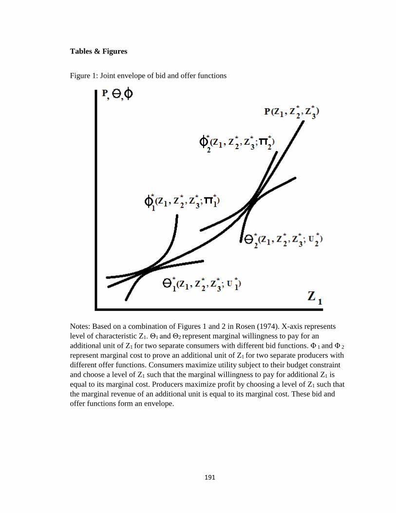
191
Tables & Figures
Figure 1: Joint envelope of bid and offer functions
Notes: Based on a combination of Figures 1 and 2 in Rosen (1974). X-axis represents
level of characteristic Z1. Θ1 and Θ2 represent marginal willingness to pay for an
additional unit of Z1 for two separate consumers with different bid functions. Φ 1 and Φ 2
represent marginal cost to prove an additional unit of Z1 for two separate producers with
different offer functions. Consumers maximize utility subject to their budget constraint
and choose a level of Z1 such that the marginal willingness to pay for additional Z1 is
equal to its marginal cost. Producers maximize profit by choosing a level of Z1 such that
the marginal revenue of an additional unit is equal to its marginal cost. These bid and
offer functions form an envelope.