Embed Size (px)
Citation preview

Valuation of Swing Options andExamination of Exercise Strategies
by Monte Carlo Techniques
Dr. Uwe Dorr
Kellogg College
University of Oxford
A thesis submitted in partial fulfillment for the MSc in
Mathematical Finance
September 29, 2003

“Valuation of Swing Options and Examination of Exercise Strategies with Monte
Carlo Techniques”
Dr. Uwe Dorr
MSc in Mathematical Finance
Trinity 2003
Abstract
Monte–Carlo simulation techniques are used to investigate (standardized)
Swing options. In a first approach, this is done by an algorithm which
is based on the Longstaff Schwartz method for American and Bermudan
options. This algorithm yields the value of the Swing option under the
assumption that the optimal exercise strategy is applied. Furthermore the
optimal strategy can be extracted from the algorithm. Various examples
including Swing options with upswings, downswings and penalties are
valued numerically, and an upper boundary for Swing options is found
in the computer experiment. In a second approach, the exercise strategy
is used as input parameter and the expected payoff with respect to this
strategy is calculated by strictly forward evolving Monte Carlo. For these
simualtions, a one factor log–normal mean–reverting process is used to
desribe the behaviour of the underlying spot price. The success of several
sample strategies is discussed in terms of process properties like mean–
reversion speed and volatility.

Contents
1 Introduction 1
1.1 Swing Options in the Real World . . . . . . . . . . . . . . . . . . . . 1
1.2 Valuation of Swing Options . . . . . . . . . . . . . . . . . . . . . . . 2
1.2.1 Modelling the Price Process . . . . . . . . . . . . . . . . . . . 3
1.2.2 Numerical Methods for the Early Exercise Problem . . . . . . 4
1.3 The Aim of This Thesis . . . . . . . . . . . . . . . . . . . . . . . . . 5
1.4 How this Thesis is Organized . . . . . . . . . . . . . . . . . . . . . . 6
2 Stochastic Processes for the Electricity Spot Price 8
2.1 One Factor Mean-Reverting Process . . . . . . . . . . . . . . . . . . . 9
2.1.1 The Process . . . . . . . . . . . . . . . . . . . . . . . . . . . . 9
2.1.2 Solution for S(t) . . . . . . . . . . . . . . . . . . . . . . . . . 10
2.1.3 Mean and Variance of S . . . . . . . . . . . . . . . . . . . . . 11
2.1.4 Vanilla Call Option . . . . . . . . . . . . . . . . . . . . . . . . 11
2.1.5 Summary . . . . . . . . . . . . . . . . . . . . . . . . . . . . . 12
2.2 Two Factor Mean–Reverting Process . . . . . . . . . . . . . . . . . . 13
2.2.1 The Process . . . . . . . . . . . . . . . . . . . . . . . . . . . . 13
2.2.2 Solution for log S(t) . . . . . . . . . . . . . . . . . . . . . . . . 14
2.2.3 Forward Price and Vanilla Call Option . . . . . . . . . . . . . 17
3 Least Squares Monte Carlo for Swing Options 18
3.1 The Longstaff–Schwartz Algorithm for American and Bermudan Options 19
3.1.1 Theory . . . . . . . . . . . . . . . . . . . . . . . . . . . . . . . 19
3.1.2 The Algorithm . . . . . . . . . . . . . . . . . . . . . . . . . . 21
3.2 Extension of Longstaff-Schwartz to Swing Options . . . . . . . . . . . 23
3.2.1 Illustrative Example . . . . . . . . . . . . . . . . . . . . . . . 23
3.2.2 General Case: Upswings, Downswings and Penalty Functions . 27
3.2.3 Implementation . . . . . . . . . . . . . . . . . . . . . . . . . . 29
i

3.3 Computational Results . . . . . . . . . . . . . . . . . . . . . . . . . . 31
3.3.1 Tests . . . . . . . . . . . . . . . . . . . . . . . . . . . . . . . . 32
3.3.2 Results for the One-Factor Process . . . . . . . . . . . . . . . 32
3.3.3 Results for the Two Factor Process . . . . . . . . . . . . . . . 35
3.3.4 Upper and Lower Boundaries . . . . . . . . . . . . . . . . . . 36
4 Exercise Strategies 45
4.1 Illustration of Early Exercise for a Bermudan Option with two Exercise
Opportunities . . . . . . . . . . . . . . . . . . . . . . . . . . . . . . . 46
4.1.1 The Threshold for Early Exercise . . . . . . . . . . . . . . . . 46
4.1.2 Dependence of the Threshold on the Process Parameters . . . 48
4.1.3 Summary of the Early Exercise Problem . . . . . . . . . . . . 50
4.1.4 Interplay between Early Exercise and Option Value . . . . . . 51
4.2 Valuation of Swing Options in Terms of Exercise Strategies . . . . . . 52
4.2.1 Optimal Strategy for Swing Options . . . . . . . . . . . . . . 53
4.2.2 Comparison of Different Exercise Strategies . . . . . . . . . . 58
5 Summary and Outlook 65
5.1 Summary . . . . . . . . . . . . . . . . . . . . . . . . . . . . . . . . . 65
5.2 Outlook . . . . . . . . . . . . . . . . . . . . . . . . . . . . . . . . . . 66
A Proof of the Statement: Threshold for Early Exercise > Mean Re-
version Level 68
B The MATLAB Routines 70
Bibliography 77
ii

Chapter 1
Introduction
1.1 Swing Options in the Real World
In order to hedge themselves against extreme price fluctuations of certain commodi-
ties, many consumers enter into forward contracts which give them the right and the
obligation to purchase a fixed amount of the commodity for a predetermined price.
However, for some market participants this reduction of risk is not sufficient, since
they do not know their exact future need of the commodity. In particular, this is a
serious problem with commodities that cannot be stored or for which storage is very
expensive.
Therefore so-called Swing contracts have been developed in order to give the holder
a certain flexibility with respect to the amount purchased in the future. These sort of
contracts are mainly found in energy markets, since energy is difficult (or expensive)
to store and exhibits extreme price fluctuations. This refers especially to electricity,
but Swing contracts appear also in coal (see [11, 12]) and gas markets (see [4]), for
example.
In the following we concentrate mainly on Swing options on electricity. The main
characteristic properties of Swing options however, i. e. the multiple early exercise
features, are the same for all underlying commodities. Only the choice of suitable
stochastic processes depends strongly on the type of underlying asset.
According to [10], typical Swing contracts contain a so called base load agreement.
The base load agreement is a set of forward contracts with different expiry dates tj,
j = 1, . . . , N . Each forward contract Fj is based on a fixed amount of electricity
(or, in general, any commodity), bj. At each expiry date the holder has the option to
purchase an excess amount or decrease the base load volume. This means the amount
of electricity purchased (for a predetermined price, i. e. the strike price) by the holder
1

of the Swing option can “swing” within a certain range (bj + ∆j) where
∆j ∈ (l1j , l2j ) ∪ (l3j , l
4j ) (1.1)
l1j ≤ l2j ≤ 0 ≤ l3j ≤ l4j (1.2)
If ∆j is positive (negative) the option exercised by the holder at opportunity tj is
called upswing (downswing).
In the case when l1j 6= l2j (or l3j 6= l4j ) the holder can choose the nominal of the
option (that means the amount to purchase for upswings or to sell for downswings)
within the respective range.
For typical contracts there a further restrictions:
• the total number of upswings, U , and downswings, D, is limited, i. e. , U ≤ N ,
D ≤ N , U + D ≤ N
• there may be a penalty payment which depends on the total volume purchased
at the end of the Swing contract period (which usually corresponds to the end
of the base load contract tN)
For valuation purposes, the base load contract on the one side and the up- and
downswings on the other side can be separated from each other. For the remainder
of this thesis we concentrate on the latter part and consider the Swing option as a
set of U upswings and D downswings, including a penalty agreement.
1.2 Valuation of Swing Options
The valuation of electricity Swing options involves two main issues:
• Modelling the underlying electricity price process;
• Solving the complex early exercise problem.
These two aspects are – in principle – independent of each other. The first has been
widely discussed in the context of futures price modelling in electricity markets, for
example. The second can be considered as an extension of Bermudan exercise features
which occur frequently in the context of interest rate derivatives like swaptions.
2

1.2.1 Modelling the Price Process
As a consequence of liberalization of electricity markets which has taken place in the
U.S. and many European countries, the energy price is mainly driven by supply and
demand. Together with some characteristic properties of electricity, this leads to large
short–term volatility of the electricity spot price. These characteristic properties can
be summarized as follows:
• Power as a commodity exhibits a heterogenous nature, both with respect to
time and location of its generation (see [13]);
• Electricity cannot be stored efficiently;
• Arbitrage processes are difficult to set up because of technical constraints (see
[5]) and thus electricity markets are not completely efficient.
In addition to pronounced short–term volatility electricity prices exhibit further
typical properties which result from the peculiarities of supply and demand:
• Mean reversion: volatility decreases with increasing time horizon. There is a
long–term equilibrium (“fair price”) which is much less volatile than the spot
price. The mean–reversion speed is determined by how quickly supply can react
on sudden demand changes (see [16]);
• Cyclical variations: these occur on different time–scales (time of day, day
of week, seasons) and are driven by cyclical demand changes. This aspect of
the price process can be considered as deterministic and therefore easily be
separated from the stochastic time dependence (see [1] where this is discussed
for a temperature process in the context of weather derivatives);
• Occasional spikes: in addition to the large short–term volatility extreme
changes occur occasionally which last only for a very short time. Positive spikes
can, e. g. , be caused by outages in the generation or transmission process (see
[7]) or by extreme events (politics, weather, etc.). Negative spikes can occur
when it is difficult to reduce generation capacity in periods of low demand.
From these observations it is clear that simple geometric Brownian motion which
is very popular for the modelling of equity prices is not well suited to model the
electricity price process.
3

Several log–normal mean–reversion processes have been proposed in the literature.
These processes can be driven by one stochastic factor, as discussed in [17] or [15], or
by two or more factors (see, for example, [8]).
These processes, however, do not cover occasional spikes completely. Therefore
jump diffusion processes are frequently used. For example, a discrete jump diffusion
component can be added to a log–normal model. In [9] and [16] two–factor mean–
reverting processes with jumps are suggested, and among practitioners three–factor
models seem to be quite popular [19].
1.2.2 Numerical Methods for the Early Exercise Problem
Because of their complicated early exercise features, Swing options can be considered
as a generalization of Bermudan–type options which are common in interest rate
markets and thus frequently discussed in literature. A holder of a Bermudan–type
option can exercise his right only once. Further, Bermudan–type options can be
regarded as dicretized American options which are very popular in equity markets,
for example.
In general, there is no analytical solution for the early exercise problem and thus
numerical methods have to be applied.
For Swing options, tree–based methods as suggested in [10] seem to be the most
popular approach so far, but there are other possibilities for tackling the problem.
For example, in a recent thesis (see [18]), valuation of Swing options by finite–
differences has been demonstrated.
In the case of Bermudan options in interest markets, Monte–Carlo methods have
become popular during the last few years. There are mainly two important ap-
proaches:
• Parametrization of the early exercise decision and optimization of the strategy
as proposed in [2];
• Finding the optimal strategy by estimating the conditional continuation as
demonstrated in [14].
In the latter case, conditional continuation values are estimated via a series of
regressions. This approach is pursued in the present thesis.
4

1.3 The Aim of This Thesis
In summary, there are three main goals tracked by this thesis:
• Implementation of a tool for the valuation of Swing options which is flexible
enough to allow for different underlying stochastic processes – this valuation
corresponds to the usual optimal strategy approach;
• Monitoring expected payoffs of Swing options for different (suboptimal) exercise
strategies and comparison with the optimal strategy;
• Investigating the dependence of Swing option values, expected payoffs and opti-
mal early exercise boundaries on process parameters like mean-reversion speed
and volatility.
For these purposes, it seems to be appropriate to simplify the object under consider-
ation in two ways.
First, we restict ourselves to standardized simplified Swing contracts. The main
part of the present thesis concentrates to Swing contracts solely with upswings and
no penalties. At N exercise opportunities these contracts give the holder the right
(but not the obligation) to purchase a certain amount of the underlying for a specified
(strike) price, but the holder can exercise this right at most m times (where m ≤ N).
At each single opportunity, only one right may be exercised.
Note that the fixed exercise amount implied by this contract is no further restric-
tion in the absence of penalty agreements. If there is no penalty, the holder will
always choose the maximum amount when he exercises an up– or downswing.
Valuation of Swing contracts with upswings, downswings and penalties however
is performed as well, but without detailed discussion of the results.
Second, we consider only two different stochastic processes for the underlying.
The first is a one factor mean-reverting process which is well suited to demonstrate
of the impact of mean-reversion and volatility. Virtually all systematic investigations
of the interplay between process parameters on the one side and Swing option values,
expected payoffs or early exercise boundaries on the other side refer to this process.
In all practical computations the process components which depend determinis-
tically on time are set constant. Since deterministic effects like seasonality of prices
are beyond the scope of the present work, this means no restriction. For a discussion
of the impact of seasonality, refer to [18].
5

The second stochastic process is a two factor mean–reverting process. For this
process, valuation of Swing options is demonstrated but no discussion of the impact
of the process parameters is given.
Neither of the two processes seem to be first choice for the calibration of real mar-
ket data, since they do not cover extreme price spikes which are frequently observed
in electricity markets, for example (see above). The one factor process covers some
very important aspects of real processes like mean-reversion while the number of pa-
rameters is small enough to allow for systematic investigations. A further advantage
is that for this process the valuation of Swing options by finite-differences has been
carried out in a former thesis [18] and thus the results can be compared.
Monte Carlo simulations are chosen in this thesis, although these methods ex-
hibit some disadvantages like slow convergence and difficult handling of early exercise
features. However, the following arguments make it clear why Monte Carlo an ap-
propriate approach to the numerical valuation of Swing options:
• In this thesis it is demonstrated that the Least-Squares Monte-Carlo method
for American opions presented by Longstaff and Schwartz [14] works for Swing
options as well;
• The numerical valuation tool presented in this thesis can easily be expanded to
any stochastic process;
• Monte Carlo methods allow for monitoring the numerical uncertainty, both in
the value of the Swing option and in the early exercise thresholds;
• In addition to the Least-Squares Monte Carlo approach, expected payoffs for
different strategies can be determined very easily by Monte Carlo simulations.
1.4 How this Thesis is Organized
After this introductory chapter, the rest of the thesis is organized as follows.
In Chapter 2 the two stochastic processes under consideration are discussed with
respect to analytic solutions for the stochastic spot price, its expected value (forward
price) and the value of vanilla call options.
The Least-Squares Monte-Carlo method for the valuation of American options is
described in the first part of Chapter 3. Its extension to Swing options is introduced
in the second part where both the algorithm and its implementation are discussed.
The last part of the chapter contains numerical results obtained for both stochastic
6

processes, including the valuation of Swing options with upswings, downswings and
penalties, and the comparison with finite-differences calculations.
Exercise strategies are discussed in Chapter 4. The whole chapter is restricted to
the one factor mean-reverting process. In the first part, the early exercise problem
including the influence of the process parameters on the threshold for early exercise
are discussed in detail for the special case of a Bermudan option with two exercise
opportunities. The extension of the early exercise problem to Swing options is given
in the second part of the chapter. This includes the determination of the optimal
strategy and its convergence from Least-Squares Monte-Carlo and quantitative results
for the success of several (suboptimal) sample strategies and its dependence on the
process parameters.
7

Chapter 2
Stochastic Processes for theElectricity Spot Price
In this thesis two different stochastic processes for the spot price of electricity are
discussed explicitly. The one factor mean-reverting process described first has already
been used in a previous thesis [18]. In that thesis Swing options have been valued by
finite differences. This yields the important advantage that option values obtained
by the two different methods can be compared with each other. A further advantage
of the one factor process is the fact that there are only a few process parameters.
Systematic investigation of characteristic process properties like mean–reversion and
volatility is therefore much easier than in the case of processes with many parameters.
The second process under investigation is a two factor mean-reverting process.
Although significantly more complicated than the one factor process this process can
be integrated as well. This is advantegous since the Monte–Carlo simulation does not
need to be performed for differential timesteps.
Both processes are treated in the following manner. First, the characteristic pa-
rameters are discussed. Then the stochastic differential equation for the spot price
is solved. This yieds the spot price as a function of a stochastic variable. From this
function the expected value of the spot price, i. e. the forward price, is calculated
analytically. Finally the price of a vanilla call option is obtained by calculating the
expected value of its payoff.
8

2.1 One Factor Mean-Reverting Process
2.1.1 The Process
According to [15] we consider a process
St = F (t)eYt (2.1)
for the electricity spot price S where F (t) denotes the deterministic part and Yt the
stochastic part driven by the process
dYt = −αYtdt + σ(t)dWt (2.2)
Equation (2.2) describes a mean-reverting process with mean–reversion level zero
and mean-reversion speed α > 0. In the stochastic term of (2.2), σ(t) denotes the
time-dependent (but deterministic) volatility and dWt the increment of a standard
Brownian motion. The stochastic function Y describes the deviation from the deter-
ministic (but time–dependent) equilibrium level F .
As usually done for stock markets, exponential price changes are assumed in this
model. In particular, this assumption prevents negative prices. Furthermore, the
process (2.1) has the important advantage that it is integrable for any positive, con-
tinuously differentiable function F (t). This allows for a wide range of models for the
deterministic part of the price. The deterministic part of the price includes the effect
of seasonality which is an important property of electricity prices.
Using Ito’s lemma we obtain
dS =
(d log F (t)
dt+ α log F (t) +
1
2σ2(t)− α log S
)Sdt + σ(t)SdWt (2.3)
= α (ρ(t)− log S) Sdt + σ(t)SdWt (2.4)
where
ρ(t) =1
α
(d log F (t)
dt+
1
2σ2(t)
)+ log F (t) (2.5)
Note that the process above is assumed to be the real–world process. Since no efficient
hedging strategy exists for this contract, the Monte-Carlo simulations are performed
with the real–world process. There is no market price of risk and therefore no trans-
formation into the risk-neutral world.
9

2.1.2 Solution for S(t)
Substituting
r = log S (2.6)
and applying Ito’s lemma once again yields
dr =
(α(ρ(t)− r)− 1
2σ2(t)
)dt + σ(t)dWt (2.7)
For simplicity of notation we introduce
β(t) = αρ(t)− 1
2σ2(t) =
d log F (t)
dt+ α log F (t) (2.8)
and obtain
dr + αrdt = β(t)dt + σ(t)dWt (2.9)
Keeping in mind that
d(reαt
)= eαtdr + αreαtdt (2.10)
we can integrate (2.9) from the start point t0 to the end point t and we get
r(t) = r(t0)e−α(t−t0) +
∫ t
t0
e−α(t−s)β(s)ds +
∫ t
t0
e−α(t−s)σ(s)dWs (2.11)
With the definition (2.8) the first integral in (2.11) can be calculated explicitly. Sub-
stituting
r = log F (2.12)
and using (2.8) yields
e−α(t−s)β(s) = e−α(t−s)
(dr
ds+ αr(s)
)=
d(r(s)e−α(t−s)
)ds
(2.13)
and therefore we can rewrite (2.11)
r(t)− r(t) = (r(t0)− r(t0)) e−α(t−t0) +
∫ t
t0
e−α(t−s)σ(s)dWs (2.14)
Resubstituting r and r according to (2.6) and (2.12), respectively, we finally obtain
S(t) = F (t)
(S(t0)
F (t0)
)e−α(t−t0)
e∫ t
t0e−α(t−s)σ(s)dWs (2.15)
The integral in the exponent of the last term of (2.15) is stochastic. Since the incre-
ment dWs is normally distributed with zero mean and variance ds
dWs ∼ N(0, ds) (2.16)
10

the integral is also normally distributed with zero mean and variance
v(t, t0) := var
[∫ t
t0
e−α(t−s)σ(s)dWs
]=
∫ t
t0
e−2α(t−s)σ2(s)ds (2.17)
Thus we can write (2.15) as
S(t, t0) = A(t, t0)eX (2.18)
where
A(t, t0) = F (t)
(S(t0)
F (t0)
)e−α(t−t0)
(2.19)
and
X ∼ N(0, v(t, t0)) (2.20)
2.1.3 Mean and Variance of S
At this stage, the calculation of the expected value and the variance of S is very easy
E[S(t)|S(t0)] = A(t, t0)E[eX ] (2.21)
= A(t, t0)
∫ ∞
−∞
1√2πv(t, t0)
e− X2
2v(t,t0) eXdX (2.22)
= A(t, t0)ev(t,t0)
2 (2.23)
and the variance is given by
var[S(t)|S(t0)] = E[S2(t)|S2(t0)]− (E[S(t)|S(t0)])2 (2.24)
where
E[S2(t)|S2(t0)] = A2(t, t0)
∫ ∞
−∞
1√2πv(t, t0)
e− X2
2v(t,t0) e2XdX (2.25)
= A2(t, t0)e2v(t,t0) (2.26)
and thus
var[S(t)|S(t0)] = A2(t, t0)(e2v(t,t0) − ev(t,t0)
)(2.27)
2.1.4 Vanilla Call Option
In the next step we consider a vanilla call option with strike K and expiry time t. The
value of this option at time t0 is given by the discounted expected payoff at expiry
c(S, t0, t) = e−r(t−t0)E[max(S(t)−K, 0)|S(t0)] (2.28)
11

For simplicity, we set the risk–free interest rate to zero. This has been done in
[18] with the explanation that a risk–free portfolio containing a physically settled
derivative remains constant and does not grow with the risk–free rate.
However, typical time–horizons discussed in this thesis are in the order of magni-
tude of a couple of days. This means that discounting has virtually no effect.1
With zero interest rate we obtain
c(S, t0, t) = E[max(A(t, t0)eX −K, 0)|S(t0)] (2.29)
= A(t, t0)E[max(eX − K
A(t, t0), 0)|S(t0)] (2.30)
= A(t, t0)
∫ ∞
−∞
1√2πv(t, t0)
max(eX − K
A(t, t0), 0)e
− X2
2v(t,t0) dX (2.31)
= A(t, t0)1√
2πv(t, t0)
∫ ∞
log KA(t,t0)
(eX − K
A(t, t0)
)e
X2
2v(t,t0) (2.32)
= A(t, t0) · ev(t,t0)
2 N 0v(t,t0)(d1)−K · N 0
v(t,t0)(d2) (2.33)
where
N ab (y) =
∫ y
−∞
1√2πb
e−(x−a)2
2b dx (2.34)
is the normal cumulative function with mean a and variance b and
d1 = log
(A(t, t0)
K
)+ v(t, t0) (2.35)
d2 = d1 − v(t, t0) (2.36)
2.1.5 Summary
In summary, using the notation
A(t, t0) = F (t)
(S(t0)
F (t0)
)e−α(t−t0)
(2.37)
v(t, t0) =
∫ t
t0
e−2α(t−s)σ2(s)ds (2.38)
d1 = log
(A(t, t0)
K
)+ v(t, t0) (2.39)
d2 = d1 − v(t, t0) (2.40)
we have found the following expressions for the spot price, the forward price and the
value of a vanilla call option.
1Note that typical values for the daily volatility are in the order of 40%. This will completelycover up the discounting effect.
12

Spot Price
The spot price at time t given the spot price at time t0 is
S(t, t0) = A(t, t0)eX (2.41)
X ∼ N(0, v(t, t0)) (2.42)
Forward Price
The forward price of S at time t0 with respect to expiry t is given by
F(S, t0, t) = A(t, t0)ev(t,t0)
2 (2.43)
Vanilla Call Option
The value at time t0 of a vanilla call option with strike K and expiry t is given by
c(S, t0, t) = A(t, t0) · ev(t,t0)
2 N 0v(t,t0)(d1)−K · N 0
v(t,t0)(d2) (2.44)
In the special case of constant F and constant volatility, i. e.
F (t) ≡ F = const (2.45)
σ(t) ≡ σ = const (2.46)
we obtain
A(t, t0) = S(t0)e−α(t−t0)
F 1−e−α(t−t0)
(2.47)
v(t, t0) =σ2
2α
(1− e−2α(t−t0)
)(2.48)
2.2 Two Factor Mean–Reverting Process
2.2.1 The Process
According to [8] we consider the following process:
dSt = (r − δt)Stdt + σSStdW St (2.49)
where r is the interest rate and σS the variance of the geometric Brownian motion
followed by S. The convenience yield δt is stochastic and follows a mean–reverting
process
dδt = α(κδ − δt)dt + σδdW δt (2.50)
13

The variance of the change of the convenience yield is represented by σδ, αδ is the
speed of adjustment and κδ the long–run mean yield. Furthermore, the two Wiener
processes W St and W δ
t are correlated with correlation coefficient ρ.
Since the concept of convenience yield is usually only applied to storable com-
modities, this model is more appropriate for gas or oil prices than for electricity.2
Nevertheless is it relevant for Swing options in general.
In this approach the net convenience yield can be interpreted as a theoretical
construction to incorporate the special effects of supply, demand and other particu-
liarities of the power market into one variable. Those effects are usually stochastic,
implying a model for the stochastic behaviour of convenience yield. As a key as-
sumption in the model, electricity is therefore modelled as an asset with stochastic
(positive or negative) dividend yield δt which itself follows a mean–reversion process
of the Ornstein–Uhlenbeck type.
For simplicity, the market price of convenience yield risk is assumed to be zero.
2.2.2 Solution for log S(t)
If we consider B(S, δ, t) to be a twice continuously differentiable function, we obtain
from Ito’s lemma
dB = BSdS + Bδdδ + Btdt +1
2BSS (dS)2 +
1
2Bδδ (dδ)2 + BSδdSdδ (2.51)
where the subscripts denote the respective partial derivatives (see [8]).
With B(S, δ, t) = log S and (2.49) we obtain immediately
d log St = (r − δt −1
2σ2
S)dt + σSdW St (2.52)
Integration from t0 to t yields
log St = log St0 +
(r − 1
2σ2
)(t− t0)−
∫ t
t0
δ(y)dy + σS
∫ t
t0
dW Ss (2.53)
Equation (2.50) can be written as
dδt + αδtdt = ακδdt + σδdW δt (2.54)
Using (2.10) this can be integrated and we obtain
δ(y) = κδ + (δt0 − κδ)e−α(y−t0) + σδ
∫ y
t0
e−α(y−s)dW δs (2.55)
2Note that in [8] the two–factor model was applied to oil prices.
14

and thus∫ t
t0
δ(y)dy = κδ(t− t0) + (δt0 − κδ)1− e−α(t−t0)
α+ σδ
∫ t
t0
∫ y
t0
e−α(y−s)dydW δs (2.56)
The integral on the right hand side of (2.56) can be written as∫ t
t0
[e−αy
∫ y
t0
eαs dW δs
dsds
]dy (2.57)
and therefore it can be evaluated using integration by parts. As final result for the
integral over δ we obtain∫ t
t0
δ(y)dy = κδτ + (δt0 − κδ)1− e−ατ
α+ σδ
∫ t
t0
1− e−α(t−s)
αdW δ
s (2.58)
where τ = t− t0. Equation (2.53) can now be rewritten as
log St = log St0 +
(r − 1
2σ2
S − κδ
)τ − (δt0 − κδ)
1− e−ατ
α+ X − Y (2.59)
where the stochastic variables X and Y are given by
X = σS
∫ t
t0
dW Ss = σS
(W S
t −W St0
)(2.60)
Y = σδ
∫ t
t0
1− e−α(t−s)
αdW δ
s (2.61)
Since the increments dW S and dW δ are correlated, X and Y are correlated as well.
Provided that X and Y are not perfectly correlated or anticorrelated3 we can decor-
relate the random variables by performing the transformation(dW S
dW δ
)=
1√2
(1 −11 1
)(dX ′
dY ′
)(2.62)
The transformed increments dX ′ and dY ′ are uncorrelated and their variances are
given by
E[dX ′dX ′] = (1 + ρ)dt (2.63)
E[dY ′dY ′] = (1− ρ)dt (2.64)
With the new increments we obtain
X ′ =1√2
∫ t
t0
[σS −
σδ
α(1− e−α(t−s))
]dX ′
s (2.65)
Y ′ =1√2
∫ t
t0
[σS +
σδ
α(1− e−α(t−s))
]dY ′
s (2.66)
3In this case the process could be regarded as a one–factor process.
15

Equation (2.55) can be written as
δt = κδ + (δt0 − κδ)e−ατ + Z (2.67)
where the random variable Z is given by
Z = σδ
∫ t
t0
e−α(t−s)dW δs (2.68)
=σδ√2
∫ t
t0
e−α(t−s)dX ′s +
σδ√2
∫ t
t0
e−α(t−s)dY ′s (2.69)
= Z ′X + Z ′Y (2.70)
There is full correlation between X ′ and Z ′X , and between Y ′ and Z ′Y . The variances
of the random variables can be calculated by evaluating the following integrals;
var[X ′] =1 + ρ
2
∫ t
t0
[σS −
σδ
α(1− e−α(t−s))
]2ds (2.71)
var[Y ′] =1− ρ
2
∫ t
t0
[σS +
σδ
α(1− e−α(t−s))
]2ds (2.72)
var[Z ′X ] =1 + ρ
2
∫ t
t0
σ2δe−2α(t−s)ds (2.73)
var[Z ′Y ] =1− ρ
2
∫ t
t0
σ2δe−2α(t−s)ds (2.74)
In summary we obtain the following results:
log St = log St0 + β(τ) + X ′ − Y ′ (2.75)
δt = η(τ) + Z ′X + Z ′Y (2.76)
where
β(τ) = (r − 1
2σ2
S − κδ)τ − (δt0 − κδ)1− e−ατ
α(2.77)
η(τ) = κδ + (δt0 − κδ)e−ατ (2.78)
τ = t− t0 (2.79)
The random variables X ′, Y ′, Z ′X and Z ′Y are normally distributed with mean zero
and their variances are given by
var[X ′] =1 + ρ
2
[γ2−τ + 2γ−
σδ
α2(1− e−ατ ) +
σ2δ
2α3(1− e−2ατ )
](2.80)
var[Y ′] =1− ρ
2
[γ2
+τ − 2γ+σδ
α2(1− e−ατ ) +
σ2δ
2α3(1− e−2ατ )
](2.81)
var[Z ′X ] =1 + ρ
4ασ2
δ (1− e−ατ ) (2.82)
var[Z ′Y ] =1− ρ
4ασ2
δ (1− e−ατ ) (2.83)
16

where
γ± = σS ±σδ
α(2.84)
2.2.3 Forward Price and Vanilla Call Option
We can rewrite (2.75) as
S(t) = S(t0)eβ(τ)eχ (2.85)
where the new random variable
χ = X ′ − Y ′ (2.86)
is normally distributed with mean zero and variance
var[χ] ≡ vχ = var[X ′] + var[Y ′] (2.87)
where var[X ′] and var[Y ′] are given by (2.80) and (2.81), respectively. Thus we can
calculate the forward price and the price of a vanilla call option according to (2.23)
and (2.33), respectively, and obtain the following results:
Forward Price
The forward price of S at time t0 with respect to expiry t is given by
F(S, t0, t) = S(t0)eβ(τ)e
vχ2 (2.88)
where β(τ) and vχ are given by (2.77) and (2.87), respectively.
Vanilla Call Option
The value at time t0 of a vanilla call option with strike K and expiry t is given by
c(S, t0, t) = S(t0)eβ(τ)e
vχ2 N 0
vχ(d1)−KN 0
vχ(d2) (2.89)
where
d1 = β(τ) + log
(S(t0)
K
)+ vχ (2.90)
d2 = β(τ) + log
(S(t0)
K
)(2.91)
and N ba (·) is given by (2.34).
17

Chapter 3
Least Squares Monte Carlo forSwing Options
Monte–Carlo methods are very popular in practical finance, since they are – in general
– easy to implement and allow the treatment of problems with high dimensionality.
In particular, when there are multiple stochastic factors, numerical methods like
finite–differences or binomial techniques become impractical while Monte Carlo is
still appropriate. Since the convergence of Monte Carlo is fairly slow, other methods
are preferred as long as the underlying stochastic process is simple and the number
of risk factors is small.
In the case of energy derivatives appropriate stochastic processes for the underly-
ing, e. g. the electricity price, are in general considerably complicated, since they have
to account for seasonality, mean reversion, spikes etc (see §1.2.1). Calibration of a
model for the energy price to real market data usually requires at least two stochas-
tic factors, frequently in conjunction with jump diffusion. Therefore Monte–Carlo
methods may be the best choice if the stochastic processes under consideration are
expected to be close to reality.
However, the treatment of early exercise features is a great challenge for Monte–
Carlo methods. For American and Bermudan options several approaches to this
problem have been discussed in the literature. Some authors use stratification or
parametrization techniques to approximate the transitional density function or the
early exercise boundary (see references in [14]). Others treat the problem in a different
way. They focus directly on the conditional expectation function involved in the
iterations of dynamic programming and use least squares regression to estimate the
conditional expectations. These conditional expectations, i. e. the continuation values
under the asumption that the option is not exercised at a particular opportunity
(iteration step) are estimated by least squares regression.
18

One example for these Least Squares Monte Carlo (LSM) methods is the algorithm
proposed by Longstaff and Schwartz [14] which seems to have become more and more
popular among practitioners [6]. In the first part of the present chapter the Longstaff
Schwartz algorithm for American or Bermudan options is described.
The extension of this algorithm to Swing options with more than one exercise
right is discussed in the second part, including the presence of upswings, downswings
and penalty functions. As a central issue of the present thesis the extended algorithm
has been implemented in MATLAB and the routines involved are sketched in this
part.
The third part addresses some computational results which have been obtained
using the routines outlined in the second part of this chapter. These results include
simulations for both the one factor and the two factor processes described in Chapter
2. In particular, an upper bound for Swing options is obtained from the numerical
experiment.
3.1 The Longstaff–Schwartz Algorithm for Amer-
ican and Bermudan Options
3.1.1 Theory
The basic idea of the Longstaff Schwartz algorithm, described in detail in [14] (and
similar approaches like those reported in [6]), is to use least squares regression on a
finite set of functions as a proxy for conditional expectation estimates.
In a first step, the time axis has to be discretized, i. e. if the American option is
alive within the time horizon [0, T ] early exercise is only allowed at discrete times
0 < t1 < t2 < . . . < tJ = T . The American option is thus approximated by a
Bermudan option.
For a particular exercise date tk, early exercise is performed if the payoff from
immediate exercise exceeds the continuation value, i. e. the value of the (remaining)
option if it is not exercised at tk. This continuation value can be expressed as condi-
tional expectation of the option payoff with respect to the risk neutral pricing measure
Q. The expectation is taken conditional on the information set Ftk which is available
at tk. Representing the continuation value for a particular sample path ω by F (ω, tk)
we can write
F (ω, tk) = EQ
[K∑
j=k+1
D(tk, tj)C(ω, tj, tk, T )|Ftk
](3.1)
19
where D(tk, tj) is the discount factor from tk to tj and C(ω, tj, tk, T ) denotes the path
of cashflows generated by the option, conditional on the option not being exercised
at or prior to time tk and the holder following the optimal exercise strategy for all
remaining opportunities tj between tk and T . Note that for each path ω there is at
most one j with C(ω, tj, tk, T ) > 0, since the Bermudan option has only one exercise
right.
Starting at tJ we work backwards through time. The early exercise decision at
time tJ−1 is made by comparing F (ω, tK−1) with the immediate payoff P (X) where
X is the value of the underlying at time tJ−1 in path ω. While P (X) is known the
functional form of F (ω, tJ−1) is unknown.
Assuming some technical details, the conditional expectation can be represented
by a set of basis functions Bj as
F (ω, tK−1) =∞∑
j=0
aj(tK−1)Bj(X) (3.2)
Since we consider a Markov process for the state variable X, only current realizations
of it can be included in the basis functions Bj. For practical purposes F (ω, tJ−1) has
to be approximated by FM(ω, tJ−1) using the first M < ∞ basis functions.
At this stage the crucial step is to be done, namely estimating FM(ω, tJ−1) by
regressing the discounted values of C(ω, s, tJ−1, T ), i. e. the cashflows which occur at
tJ – onto the basis functions. Since the early exercise decision is only relevant for those
paths where the option is in the money at tJ−1 the regression is restricted to these
paths. This regression yields FM(ω, tJ−1) as an (unbiased) estimator for FM(ω, tJ−1).
Now the exercise decision is made by comparing P (X) with FM(ω, tJ−1) and with
these new cashflows at tJ−1 the iteration steps further backwards in time (see next
section). At the end the result obtained by Least–Squares Monte Carlo, V NLSM, is the
average over the cashfows from each path (note that there is at most one cashflow
per path),
V NLSM =
1
N
N∑i=1
CLSM(ωi) (3.3)
where CLSM(ωi) denotes the discounted cashflows which result from following the LSM
strategy.
Since the LSM method represents one particular strategy the “real” option value
V (which represents the optimal strategy) must be greater than or equal to V NLSM. The
convergence of V NLSM, i. e. the proposition that for any ε > 0 there exists an M < ∞
20

such that
limN→∞
Pr[|V − V N
LSM| > ε]
= 0 (3.4)
is proved mathematically by the authors of [14] for the case where there are only two
exercise opportunities. A general proof of the convergence of the Longstaff Schwartz
algorithm has been given in [6].
3.1.2 The Algorithm
In this section the Longstaff Schwartz algorithm is desribed explicitly. For the sake
of simplicity it is assumed that all interest rates are zero and therefore discounting
can be omitted. We will use this assumption throughout the rest of the thesis (see
§2.1).
Before starting the actual algorithm the paths for the underlying spot prices have
to be sampled. For N paths and J exercise opportunities (timesteps), this yields an
N × J matrix S where the matrix element Sij is the spot price in the i-th path at
time tj.
As a second preparation step the set of basis functions (Bj)Mj=0 for the regression
has to be chosen from a great variety of possibilities such as Hermite, Legendre,
Chebyshev, Gegenbauer or Jacobi polymomials, for example. However, Longstaff and
Schwartz emphasize that their numerical tests indicate that Fourier or trigonometric
series and even simple powers of the state variables also give accurate results.
The initial step of the actual algorithm is to determine the cashflow vector CJ at
the last timestep tJ . These cashflows are easy to get since the continuation values
are then zero, i. e.
CJi = P (SiJ) (3.5)
where P is the payoff function. In the following we focus on the payoff of a vanilla
call option
P (Sij) = max(Sij −Kj, 0). (3.6)
where the strike prices Kj can vary from timestep to timestep.
Second, we consider the spot prices at timestep tJ−1 and select those for which
P (SiJ−1) > 0. This yields the LJ−1 × 1–vector SJ−1 where LJ−1 is number of in-
the-money paths at timestep tJ−1. The least squares regression of CJ onto the basis
functions Bj is now performed by minimizing the expression
||BJ−1aJ−1 − CJ || (3.7)
21

where aJ−1 is the (M + 1)× 1–vector of regression coefficients for timestep tJ−1 and
the matrix BJ−1 is given by
BJ−1 =
B0(S1J−1) · · · BM(S1J−1)... · · · ...
B0(SLJ−1J−1) · · · BM(SLJ−1J−1)
(3.8)
The solution of the minimization is given by
aJ−1 =((BJ−1)T BJ−1
)−1(BJ−1)T CJ−1 (3.9)
With that we obtain the vector of continuation values ContJ−1 by
ContJ−1i =
M∑k=0
aJ−1k BJ−1
ik (3.10)
Once we have the continuation values we perform early exercise whenever
P (SiJ−1) > ContJ−1i (3.11)
The elements CJ−1i of the cashflow vector CJ−1 are then given by
• P (SiJ−1) if the early exercise condition (3.11) is true
• 0 else
Subsequently the elements of the cashflow vector CJ have to be set to zero for
those paths where (3.11) is true.
We then step backwards through time until we reach the first timestep. At each
timestep early exercise is performed as described above. Note that whenever a cash-
flow at timestep tk is generated by early exercise in path i all cashflows which occur
in this path later than tk (this is at most one) have to be removed.
At the end we can build the cashflow matrix C from the cashflow vectors Ck by
concatenating the cashflow vectors Ck, k = 1, . . . , J and the option value is given by
the artithmetic average of the row sums.1
In [14] a very helpful illustration of the algorithm is given by a numerical example.
1These sums have at most one non-zero addend.
22

3.2 Extension of Longstaff-Schwartz to Swing Op-
tions
For the valuation of Swing options the basic concepts of Least–Squares Monte Carlo
can be directly adopted. Since we now have more than one exercise right, however,
we have to deal with an additional “dimension”, i. e. the number of exercises left.
In order to avoid overformalization the extension of LSM to Swing options is first
described using a particular example, i. e. a Swing option with 5 opportunities and
3 exercise rights (upswings). After this the algorithm is generalized by introducing
downswings and penalty functions. In the last part of this section the MATLAB
implementations of the algorithms are sketched.
3.2.1 Illustrative Example
We consider a Swing option with exercise opportunities at times t1, t2, t3, t4 and t5.
There are 3 upswings, and the strike price at each opportunity is K.
Sampling N paths yields the N × 5-spot price matrix S.
The main difficulties arising from the presence of more than one exercise rights are
the following:
• The benefit from immediate exercise is not only the payoff, but the payoff plus
the value of the remaining Swing option (which has one upswing fewer than the
original one);
• When early exercise is performed at tk, rearranging the cashflows at later op-
portunities requires the cashflow matrix of the Swing option with one upswing
less than the original one.
The generalized cashflow matrix of our algorithm must therefore have three di-
mensions:
• First dimension: number of paths
• Second dimension: number of timesteps (exercise opportunity)
• Third dimension: number of exercise rights (upswings) left
We denote the cashflow matrix for e upswings2 left as Ce. In our example, there
are thus three N × 5 matrices C1, C2 and C3.
2Note that e is here an integer and not the base of natural logarithms
23

After the initial step the cashflow matrices look as follows:
C3 =
% % P (S13) P (S14) P (S15)% % P (S23) P (S24) P (S25)...
......
......
% % P (SN3) P (SN4) P (SN5)
(3.12)
C2 =
% % % P (S14) P (S15)% % % P (S24) P (S25)...
......
......
% % % P (SN4) P (SN5)
(3.13)
C1 =
% % % % P (S15)% % % % P (S25)...
......
......
% % % % P (SN5)
(3.14)
where
P (S) = max(S −K, 0) (3.15)
is the payoff of the upswing. The %–signs mean that these cashflows are undefined
at this stage.
For C3 we can combine the last three timesteps in the initial step of the algorithm
since it is obvious that early exercise takes place at t3 whenever the payoff at this
timestep is positive. Note that this is the third timestep from the last.
Similarly, when two upswings are left immediate early exercise is performed at t4
and thus we can combine the last two timesteps for C2.
The matrix C1 corresponds to the cashflow matrix in the Longstaff Schwartz
algorithm for Bermudan options.
As an example, if we have only six paths, after the initial step the matrices might
look as follows:
C3 =
% % P13 0 P15
% % P23 P24 0% % P33 0 0% % P43 P44 P45
% % P53 0 P55
% % P63 P64 P65
(3.16)
24

C2 =
% % % 0 P15
% % % P24 0% % % 0 0% % % P44 P45
% % % 0 P55
% % % P64 P65
(3.17)
C1 =
% % % % P15
% % % % 0% % % % 0% % % % P45
% % % % P55
% % % % P65
(3.18)
Here all Pij = P (Sij) are non zero.
We now start stepping backwards in time. For t4 we calculate the continuation
values for one upswing left by least squares regression of the cashflow vector C15 onto
the basis functions as described in §3.1.2. In C15 only the paths where the payoff at
t4 is positive are considered (see also §3.1.2). We denote the vector of continuation
values at timestep four with one upswing left as Cont14.
With the continuation values we can perform early exercise and C1 may look like
C1 =
% % % 0 P15
% % % P24 0% % % 0 0% % % P44 0% % % 0 P55
% % % P64 0
(3.19)
In our example, early exercise at t4 was carried out for all possible paths, i. e. paths
2, 4 and 6. Note that for paths 4 and 6 the cashflows at t5 had been removed. The
cashflow matrices C2 and C3 remain unchanged in this step.
Now we move on to t3. In order to get Cont23 we first have to add the cashflow
vectors C24 and C2
5 . Denoting the sum vector as C24+5 we obtain the relevant sum
vector C24+5 by omitting all paths where P (Si3) is zero. The continuation vector
Cont23 is then obtained by linear regression of C2
4+5 on the basis functions.
The early exercise condition now reads
P (Si3) + Cont13(i) > Cont2
3(i) (3.20)
That means we have to calculate Cont13 before we can perform early exercise in C2.
This calculation is easily done according to the usual Longstaff Schwartz algorithm.
25

For those paths where condition (3.20) is fulfilled early exercise is performed. This
means that for each corresponding path i, C23(i) is set equal to the payoff P (Si3) and
the cashflows C24(i) and C2
5(i) are replaced by C14(i) and C1
5(i), respectively.
After this early exercise for t3 is performed in C1. While C3 still remains un-
changed in this step the other cashflow matrices in our example might look like
C2 =
% % P13 0 P15
% % P23 P24 0% % P33 0 0% % 0 P44 P45
% % 0 0 P55
% % P63 P64 0
(3.21)
C1 =
% % 0 0 P15
% % P23 0 0% % 0 0 0% % 0 P44 0% % 0 0 P55
% % P63 0 0
(3.22)
For C2 early exercise was performed in paths 1, 2, 3 and 6. Note that in path 6 the
cashflows after t3 had to be modified according to C1 at the iteration step before, i. e.
t4 (see §3.19). For C1 early exercise occurs only in paths 2 and 6.
Moving on to t2 early exercise must be performed for all three cashflow matrices.
First, the continuation vectors are calculated by regressing Ce3+4+5, e = 1, 2, 3 onto
the basis functions as described above. Then early exercise is carried out starting
with C3 by evaluating the condition
P (Si2) + Cont22(i) > Cont3
2(i). (3.23)
The condition for C2 reads
P (Si2) + Cont12(i) > Cont2
2(i) (3.24)
and for C1 we obtain
P (Si2) > Cont12(i) (3.25)
Since early exercise includes rearranging the cashflows after t2 according to the cash-
flow matrix (with one upswing fewer) at the preceding iteration step, it is important
that the procedure is first done with C3, then with C2 and finally with C1.
Repeating the same procedure for t1, we end up with the final cashflow matrices
C1, C2 and C3. From these matrices we obtain the value of the corresponding Swing
options by taking the average of the row sums.
26

Note that although we were only interested in the option with 3 upswings at the
beginning, we now have valued simultaneously the options with one and two exercise
rights.3 This is very helpful with respect to the investigation of upper and lower
boundaries (see §3.3.4)
3.2.2 General Case: Upswings, Downswings and Penalty Func-tions
The general form of Swing options as described in §1.1 is more complicated since
Swing options can include, for example,
• not only call (upswings) but also put features (downswings)
• penalty functions which depend on the total number of exercises (upswings and
downswings)
This has two main consequences for the algorithm. First, in the initial step only
the last timestep can be treated since continuation values might be negative because
of penalty and thus it could be sensible to let one or more exercise rights expire
worthless. Second, we have an additional dimension, i. e. the number of downswings
left.
Let us first introduce some notation:
• u and d are the numbers of upswings and downswings exercised,4 respectively
(in a particular iteration step)
• umax and dmax are the total numbers of upswings and downswings, respectively
• J is the number of timesteps (exercise opportunities)
The generalized cashflow tensor has now four dimensions (path, timestep, up-
swings exercised, downswings exercised) and consists of [(umax + 1) · (dmax + 1)− 1]
cashflow matrices5 Cu,d. Each of these matrices has dimension (N × J).
In the initial step, we have to evaluate the cashflows at the last exercise opportu-
nity. With φ(u, d) denoting the penalty function for u upswings and d downswings
3It would not have been necessary to carry out early exercise for C2 and C1 at t1 in order to getC3, but omitting these steps implies no big improvement of computational efficiency.
4Note that in the previous Section we have used the number of exercise rights left5We do not need to calculate Cumax,dmax since this matrix is zero
27

exercised we obtain the following cashflows in path i at the final timestep tJ :
for 0 ≤ u < umax, 0 ≤ d < dmax:
Cu,dJ (i) = max [Pu(SiJ)− φ(u + 1, d), Pd(SiJ)− φ(u, d + 1), 0] (3.26)
for 0≤ d < dmax:
Cumax,dJ (i) = max [Pd(SiJ)− φ(umax, d + 1), 0] (3.27)
for 0 ≤ u < umax:
Cu,dmax
J (i) = max [Pu(SiJ)− φ(u + 1, dmax), 0] (3.28)
where Pu,d is the payoff of the up-, downswing.
Stepping backwards in time we have to do the following in each step:
• calculate the continuation values by least squares regression;
• perform early exercise.
When performing early exercise we have to step forward from u, d = 0 to u, d =
umax, dmax. It does not matter whether we start with u or d, however. Explicitly, in
timestep j (and thus iteration step J + 1 − j) the early exercise conditions for the
upswings are
for 0 ≤ u < umax, 0 ≤ d ≤ dmax, u + d < j:
Pu(Sij) + Contu+1,dj (i) > Contu,d
j (i) (3.29)
For the downswings we obtain
for 0 ≤ u ≤ umax, 0 ≤ d < dmax, u + d < j:
Pd(Sij) + Contu,d+1j (i) > Contu,d
j (i) (3.30)
Eventually the value of the Swing option is obtained by calculating the average
of the row sums of C0,0 after the final iteration step. Note that in each row there are
at most umax + dmax non-zero cashflows.
28
3.2.3 Implementation
The implementation was performed in MATLAB. Since this software is matrix-based,
matrix operations are optimized with respect to computational speed. In the par-
ticular case of Monte–Carlo simulations, one therefore has to avoid any loop over
the paths but rather handle the sampled paths as matrices. A further advantage of
MATLAB is the fact that it provides a great variety of pre-implemented numerical
operations, in particular linear (least-squares) regression.
The implementation of the extended Longstaff-Schwartz (LS) algorithm consists
of two main parts:
• the sampling of the paths;
• the least-squares algorithm.
These two parts are independent of each other and hence it is very easy to extend
the tools presented below to any stochastic process desired. In this case only the
sampling routine has to be modified. For the present thesis I have implemented two
sampling routines, one for the one factor mean-reverting process described in §2.1
and the other for the two factor-process discussed in §2.2.
I have implemented two different routines for the LS algorithm with and without
penalty functions. The reason for this is that some iteration steps are redundant if
there is no penalty (see §3.2.1) and this can be used to improve computational speed.
As we will see later, most of the results presented in this thesis are restricted to the
absence of penalty functions.
In both cases simple powers up to M = 2 are used as basis functions, i. e.
B0(X) = 1 (3.31)
B1(X) = X (3.32)
B2(X) = X2 (3.33)
In the following the most important routines are sketched very briefly. An overview
over all relevant routines which have been implemented in the context of this thesis
is given in Appendix A.
Path Sampling for the One Factor Process
Since the effects of seasonality are not in the focus of the present thesis, the deter-
ministic part F (t) in (2.1) and the volatility in (2.2) are assumed to be constant,
according to (2.45) and (2.46), respectively.
29

For the one-factor process antithetic sampling is performed. If there are N paths
and J exercise opportunities, N2×J random numbers xij are drawn independently from
a standard normal distribution. This yields a N2× J–matrix which is concatenated
with −xij along the first dimension (rows), i. e. we obtain an N×J–matrix of standard
normally distributed random numbers.
Multiplication of each column vector (x)j with√
v(tj, tj−1) where v(t, t0) is given
by (2.48) yields a matrix Xij of normally distributed random numbers with mean zero
and variance v(tj, tj−1). According to (2.41), the spot-price matrix is then obtained
from this matrix by element-wise taking the exponential and subsequent multiplica-
tion of each column vector with A(tj, tj−1) as given by (2.47).6
Path Sampling for the Two Factor Process
As above we consider N paths and J exercise opportunities. In the case of the two
factor process we have to sample two matrices x′ and y′ where the random numbers
x′ij and y′ij are uncorrelated, i. e. for each 1 ≤ i, k ≤ N and 1 ≤ j, l ≤ J we have
E[x′ijy′kl] = 0 (3.34)
From x′ and y′ we obtain the matrices X ′, Y ′, Z ′X , and Z ′Y by multiplication of the
column vectors according to
(X ′)j = var[X ′](tj) · x′j (3.35)
(Y ′)j = var[Y ′](tj) · y′j (3.36)
(Z ′X)j = var[Z ′X ](tj) · x′j (3.37)
(Z ′Y )j = var[Z ′Y ](tj) · y′j (3.38)
where the variances are given by (2.80) to (2.83), respectively.
For each timestep tj, the vectors Stj and δtj are then calculated according to (2.75)
and (2.55), respectively, where the start values δt0 and log St0 are used to calculate
the δt1 and log St1 , and the δtj−1and log Stj−1
are used to compute the δtj and log Stj .
In the last step the spot price matrix S is obtained by taking element-wise the
exponential of log S.
6Note that this is an iterative process, i. e. Stj cannot be calculated until Stj−1 is known.
30

LS Algorithm for Upswings without Penalty
As explained in §3.2.1 early exercise is performed over as many timesteps as possible
in the initial iteration step. If the total number of upswings is U all cashflow matrices
from 1 to U exercises left are calculated in the subsequent iteration steps. For each
timestep a different strike can be chosen.
LS Algorithm for Upswings and Downswings with Penalty
While upswings correspond to call option features, downswings are the put option
equivalent. The LS algorithm for downswings is completely analogous to that for
upswings, except the fact that the payoff function is the payoff of a put option. In
the actual implementation the strikes for the downswings can be chosen independently
of the strikes for the upswings.
The presence of a penalty function implies that the initial iteration steps can only
cover one (i. e. the last) timestep. This means that there are more linear regressions
to be performed and therefore the algorithm is slightly slower. In contrast to the case
of no penalty only the result for the total number of up- and downswings is returned
by the routine.
Empirical Error
In both routines the extended Longstaff Schwartz (LS) algorithm is carried out 10
times. The mean and the standard deviation of the 10 results are returned as the
option’s value and as a measure for its statistical error, respectively.
3.3 Computational Results
This section contains some results obtained by the routines described above. In order
to make sure that the routines yield correct results a number of numerical tests have
been applied to them. This is outlined in the first part of this section.
In the second and third parts some numerical results for the one and two factor
processes are presented and the influence of penalty functions is discussed.
A discussion of upper and lower boundaries for Swing options is given in the last
part of this section. In particular, an upper boundary has been found in the computer
experiment. This upper boundary is smaller than the set of Bermudan options which
is frequently referred to in the literature.
31

spot value S 20timesteps 10time between two timesteps δt 1exercise rights (upswings) 6strike at each timestep K 20mean reversion speed α 0.5mean reversion level F 20.7387volatility σ 0.392
Table 3.1: One factor mean–reverting process parameters for the convergence check.
3.3.1 Tests
The first step of the testing process concentrates on the sampling routines. A large
number of paths (usually 1000000) was sampled and the mean and variance of the
sampled spot prices have been compared with the theoretical values.
In the next step the LS routines have been applied to a vanilla call option, i. e.
one timestep (exercise opportunity) and one upswing. The result was compared with
the theoretical values as given by (2.44) and (2.89).
Up to this stage there have been no least squares regressions, i. e. the actual
Longstaff Schwartz algorithm has not proved its accuracy yet. In order to achieve
this, numerical results for the one factor process have been compared with those
obtained by finite-differences as described in [18] (see §3.3.2 below). Note that the
LS routine is independent of the sampling. This means that if the algorithm works
for the one factor process, it works for the two factor process as well.
The two different LS routines have been tested against each other, i. e. the routine
for up- and downswings with penalty has been applied to the special case of zero
penalty and zero downswings.
All tests have shown positive results.
3.3.2 Results for the One-Factor Process
Convergence
In order to check the convergence of the LS algorithm the empirical error was inver-
stigated as a function of the number of paths N . As a typical property of Monte
Carlo methods the variance of the result (and thus the empirical error) is expected to
decrease like N− 12 . The process parameters of the example chosen are given in Table
3.1.
32

For small numbers of paths (up to 800) the empirical error was calculated from
100 simulations, for large numbers of paths the error was obtained by calculating the
variance of 10 simulations.
The result is depicted in Figure 3.1. In the logarithmic representation we approx-
imately obtain a straight line with ∆ log E∆ log N
≈ −12
which is expected from the square
root behaviour mentioned above. For ≈ 100000 paths we end up with an empirical
error of about 0.1%.
102
103
104
105
10−1
100
Number of Paths
Em
p.E
rror
(%
)
Figure 3.1: Empirical error as a function of the number of paths. In this logarithmicrepresentation we approximately obtain a straight line.
Numerical Results
As a first numerical experiment, the Swing options value has been calculated for
various spot prices and two different values of the mean reversion speed α (see Figure
3.2). All other process parameters were kept constant according to Table 3.1. The
impact of mean reversion is clearly discernible. For low spot prices and large α mean
reversion tends to pull the prices up to the mean reversion level which lies slightly
above the strike. Therefore the option value is quite high even for a spot price as
small as 0.01. The opposite is true for large spot prices when mean reversion pulls the
price down and thus the options value does not increase very fast with increasing spot
33

0 5 10 15 20 25 30 35 40 45 50 550
50
100
150
200
250
Spot Price
Opt
ion
Val
ue
α=0.05
α=0.5
Figure 3.2: Swing option value as function of the spot price for two different valuesof the mean reversion speed. The Swing consists of 6 upswings at 10 opportunities.
price. In the case of weak mean reversion (α = 0.05) these effects are much weaker
and therefore the option behaves more like a vanilla call option with a geometric
Brownian motion as underlying process.
Introducing four downswings in addition to the six upswings (and keeping all
other parameters constant7) must lead to an overall increase of the Swing options
value since the new option has more exercise rights while keeping all rights of the old
option. This is shown in the left part of Figure 3.3. Since the downswings are in
the money for low spot prices the option’s value as a function of the spot price now
exhibits a minimum for both values of α.
As final step we introduce a penalty function φ:
φ(v) =
50 for v ≤ −130(v − 2) for v > 20 otherwise
(3.39)
where
v = u− d (3.40)
7the strikes of the downswings were set equal to the strikes of the upswings
34

0 10 20 30 40 50 60 70 800
50
100
150
200
250
300
350
Spot Price
Opt
ion
Val
ue
α=0.05
α=0.5
0 10 20 30 40 50 60 70 800
50
100
150
200
250
300
350
Spot Price
Opt
ion
Val
ue
α=0.05
α=0.5
Figure 3.3: Swing option value as function of the spot price for two different valuesof the mean reversion speed without (left) and with penalty (right). The Swingconsists of 6 upswings and 4 downswings at 10 opportunities. As a consequence ofthe downswings the option value exhibits a minimum. Introducing a penalty leads toan overall decrease of the option value.
and u(d) is the total number of upswings (downswings) exercised. It is evident that
the penalty must lead to an overall decrease of the option value. This is shown in the
right part of Figure 3.3.
Comparison with Finite Differences
Figure 3.4 shows a typical result of the comparison between the two methods. The
relative deviations are significantly smaller than one percent and thus lie within the
numerical accuracy. For the Monte Carlo results, the accuracy is about 0.3%. How-
ever, the accuracy for the finite–difference calculations is not known exactly.
3.3.3 Results for the Two Factor Process
Convergence
The convergence check for the two factor process has been performed in the same way
as for the one factor process (see §3.3.2). Table 3.3.3 shows the process parameters
for the calculated example.
As for the one factor process we obtain an approximately linear curve for the
empirical error as a function of the number of paths with ∆ log E∆ log N
≈ −12
which indicates
the√
N−1
law for Monte Carlo simulations. However, as expected the factor of
proportionality is larger than for the one factor process. For example, we end up
with an empirical error of ≈ 0.5 % for 100000 paths which is significantly larger
35

0 10 20 30 40 50 60 70 80−1
−0.8
−0.6
−0.4
−0.2
0
0.2
0.4
0.6
0.8
1
Spot Price
Rel
ativ
e D
evia
tion
(%)
6 upswings 0 downswings
α = 0.05
0 10 20 30 40 50 60 70 80−1
−0.8
−0.6
−0.4
−0.2
0
0.2
0.4
0.6
0.8
1
Spot Price
Rel
ativ
e D
evia
tion
(%)
6 upswings 4 downswings
α = 0.5
Figure 3.4: Relative difference between the Swing option values obtained by LeastSquares Monte Carlo and Finite Differences. The calculations have been performedfor a Swing option with 10 opportunities and mean-reversion speeds of 0.05 (left, nodownswings) and 0.5 (right, 4 downswings). All other parameters are the same as inTable 3.1
than ≈ 0.1 % in the case of the one factor process. A further reason for the slower
convergence is that unlike the one factor sampling routine, no antithetic sampling is
done in the two factor routine.
Numerical Results
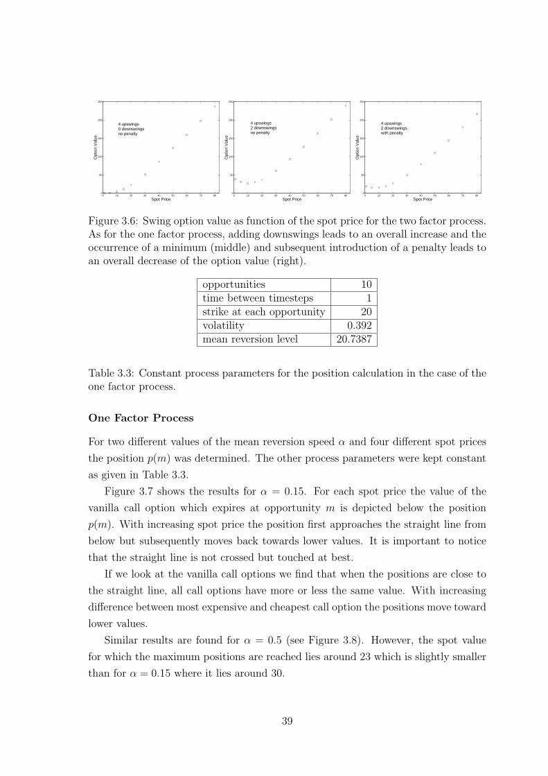
With all other parameters given in Table 3.3.3 Swing option values have been calcu-
lated for:
• six opportunities, four upswings, no downswings and no penalty;
• six opportunities, four upswings, two downswings and no penalty;
• six opportunities, four upswings, two downswings and penalty according to
(3.39)
The results are similar to those for the one factor process (see Figure 3.6).
3.3.4 Upper and Lower Boundaries
Since the numerical valuation of Swing options is – in general – quite costly, one
tries to find approximation methods which are as simple as possible. In this context
it is important to find upper and lower bounds which can be considered as a first
approximation step.
36

spot value S 20timesteps 6time between two timesteps δt 1exercise rights (upswings) 4strike at each timestep K 20α 0.5δ0 0.05κ 0.03σS 0.4σδ 0.05ρ 0.5r 0.04
Table 3.2: Two factor mean–reverting process parameters for the convergence check.For the definitions of the parameters see §2.2.1
From simple considerations one can deduce the following boundaries for a swing
option with m exercise rights and N opportunities:
• Upper boundary: m Bermudan options (each of them with N opportunities
acccording to the opportunities of the Swing option);
• Lower boundary: Callstrip, i. e. the sum of the m most valuable in the set of the
N vanilla call options which expire at the N opportunities of the Swing option.
These boundaries are frequently discussed in the literature (see [10], for example)
and can be explained in the following way:
• Upper boundary: A holder of m Bermudan options can exercise in the same
way a Swing option’s holder can. Furthermore he has the right of exercising
more than one option at the same opportunity. This means that he has more
possibilities than the holder of the Swing option and thus a set of m Bermudan
options is an upper boundary for the Swing option.
• Lower boundary: The holder of a Swing option can exercise at each opportunity
while the holder of the callstrip is restricted to m exercise dates which are fixed
at the beginning. The Swing option’s holder can exercise at these m dates, but
he doesn’t have to. Thus the callstrip must be a lower boundary.
In the next step we want to investigate where the Swing options value is situated
between the two boundaries. We therefore introduce the position p:
p =value of Swing option− lower boundary
upper boundary − lower boundary(3.41)
37

102
103
104
105
100
101
Number of Paths
Em
p. E
rror
(%
)
Figure 3.5: Empirical error as a function of the number of paths for the two factorprocess. As for the one factor process we obtain approximately a straight line In thislogarithmic representation.
It is obvious that p lies between 0 and 1. For fixed N we now consider p as a function
of m and immediately find the two trivial cases
p(1) = 1 (3.42)
p(N) = 0 (3.43)
since for m=1(N) the Swing option is the same as the Bermudan option (callstrip).
As a computer experiment, p(m) has been determined for both processes and
various sets of process parameters.
Before going into the numerical results we first have a look on the straight line
between the two limiting cases (3.42) and (3.43). This line u is given by
u(m) =N −m
N − 1(3.44)
and the position u(m) corresponds to a Swing option value Vu(m) of
Vu(m) =N −m
N − 1m · Bermudan +
m− 1
N − 1· Callstrip (3.45)
38
0 10 20 30 40 50 60 70 800
50
100
150
200
250
Spot Price
Opt
ion
Val
ue
4 upswings 0 downswingsno penalty
0 10 20 30 40 50 60 70 800
50
100
150
200
250
Spot Price
Opt
ion
Val
ue
4 upswings 2 downswingsno penalty
0 10 20 30 40 50 60 70 800
50
100
150
200
250
Spot Price
Opt
ion
Val
ue
4 upswings 2 downswings with penalty
Figure 3.6: Swing option value as function of the spot price for the two factor process.As for the one factor process, adding downswings leads to an overall increase and theoccurrence of a minimum (middle) and subsequent introduction of a penalty leads toan overall decrease of the option value (right).
opportunities 10time between timesteps 1strike at each opportunity 20volatility 0.392mean reversion level 20.7387
Table 3.3: Constant process parameters for the position calculation in the case of theone factor process.
One Factor Process
For two different values of the mean reversion speed α and four different spot prices
the position p(m) was determined. The other process parameters were kept constant
as given in Table 3.3.
Figure 3.7 shows the results for α = 0.15. For each spot price the value of the
vanilla call option which expires at opportunity m is depicted below the position
p(m). With increasing spot price the position first approaches the straight line from
below but subsequently moves back towards lower values. It is important to notice
that the straight line is not crossed but touched at best.
If we look at the vanilla call options we find that when the positions are close to
the straight line, all call options have more or less the same value. With increasing
difference between most expensive and cheapest call option the positions move toward
lower values.
Similar results are found for α = 0.5 (see Figure 3.8). However, the spot value
for which the maximum positions are reached lies around 23 which is slightly smaller
than for α = 0.15 where it lies around 30.
39

opportunities 10time between timesteps 1strike at each opportunity 20σS 0.4σδ 0.05δ0 0.05κ 0.03ρ 0.5r 0α 0.5
Table 3.4: Constant process parameters for the position calculation in the case of thetwo factor process.
Two Factor Process
For both processes the value of the vanilla call option exhibits typical behaviour. As
a consequence of mean reversion it does not necessarily increase with increasing time
to expiry. Monotonically increasing option value with increasing time to expiry is
only observed for small spot prices. For spot prices larger than the mean reversion
level the option value decreases monotonically with increasing time to expiry since
mean reversion pulls the spot price back towards the mean reversion level.
At the crossing point between increasing and decreasing behaviour the call option
value exhibits a maximum, but the dependence on the time to expiry is very weak
in this regime. With the process parameters given in Table 3.4 this crossing point
occurs for S ≈ 26. As shown in Figure 3.9 the positions are then very close to the
straight line while they move towards lower values when the spot price increases or
decreases.
Again, the straight line is not crossed and it should be emphasized that – in all
computer experiments performed for this thesis – no set of process parameters has
been found for which the position was above the straight line.
Conclusion
In computer experiments carried out for both the one factor and the two factor mean-
reverting processes, the straight line (3.45) has turned out to be an upper boundary
for Swing options. For all m, this boundary is smaller than or equal to
V Bu (m) := m · Bermudan (3.46)
40

which is frequently discussed as upper boundary in the literature. On the other hand,
with suitable process parameters, i. e. those which make all corresponding call options
worth more or less the same, the values of Swing the options are very close to the
straight line.
Unlike the boundary (3.46) there is no simple explanation why the straight line
(3.45) is indeed a theoretical boundary independent of the underlying process. In a
heuristic way, it can be interpreted as follows.
If we consider a Bermudan option (m=1) with N opportunities, we can regard
the problem as having N − 1 “degrees of freedom”, since for all opportunities except
the last one the holder can decide between early exercise and continuation. At the
last opportunity the Bermudan option is always exercised if it is in the money.
For a Swing option, there are only N −m degrees of freedom, since it has turned
into a set of m vanilla call options if no early exercise has occured before opportunity
N −m. Thus we can interpret the Swing option as consisting of Bermudan parts and
vanilla call parts. The weight of the Bermudan part is – according to the number of
’degrees of freedom’ – given by N−mN−1
and, consequently, since the weights must sum
up to 1, the weight of the vanilla call part is m−1N−1
. Since the vanilla call part can – by
definition – not be more valuable than the corresponding callstrip, (3.45) is an upper
boundary.
Assuming that the straight line is in deed an upper boundary for all underlying
processes, one can find an approximation formula for Swing options. This formula
yields some value between the callstrip and the straight line. The position between
those two boundaries must then depend on the spread between cheapest and most
expensive corresponding vanilla call option.
However, the explicit derivation of this approximation formula is beyond the scope
of this thesis, since for this purpose the investigation of a great variety of underlying
processes seems to be necessary.
41

1 2 3 4 5 6 7 8 9 100
0.1
0.2
0.3
0.4
0.5
0.6
0.7
0.8
0.9
1
Exercise rights
Pos
ition
S=10
α=0.15
1 2 3 4 5 6 7 8 9 100
0.1
0.2
0.3
0.4
0.5
0.6
0.7
0.8
0.9
1
Exercise rights
Pos
ition
S=20
α=0.15
1 2 3 4 5 6 7 8 9 100
5
10
15
20
25
30
Opportunity
Val
ue o
f van
illa
call
optio
n
S=10
α=0.15
1 2 3 4 5 6 7 8 9 100
5
10
15
20
25
30
Opportunity
Val
ue o
f van
illa
call
optio
n
S=20
α=0.15
1 2 3 4 5 6 7 8 9 100
0.1
0.2
0.3
0.4
0.5
0.6
0.7
0.8
0.9
1
Exercise rights
Pos
ition
S=30
α=0.15
1 2 3 4 5 6 7 8 9 100
0.1
0.2
0.3
0.4
0.5
0.6
0.7
0.8
0.9
1
Exercise rights
Pos
ition
S=50
α=0.15
1 2 3 4 5 6 7 8 9 100
5
10
15
20
25
30
Opportunity
Val
ue o
f van
illa
call
optio
n
S=30
α=0.15
1 2 3 4 5 6 7 8 9 100
5
10
15
20
25
30
Opportunity
Val
ue o
f van
illa
call
optio
n
S=50
α=0.15
Figure 3.7: Position between upper and lower boundary as a function of the numberof exercise rights. Beneath each position graph the values of the vanilla call optionsexpiring at each opportunity are depicted. The positions are close to the straight linewhen the call option values are more or less the same for all expiry dates.
42

1 2 3 4 5 6 7 8 9 100
0.1
0.2
0.3
0.4
0.5
0.6
0.7
0.8
0.9
1
Exercise rights
Pos
ition
S=10
α=0.50
1 2 3 4 5 6 7 8 9 100
0.1
0.2
0.3
0.4
0.5
0.6
0.7
0.8
0.9
1
Exercise rights
Pos
ition
S=23
α=0.50
1 2 3 4 5 6 7 8 9 100
2
4
6
8
10
12
14
16
Opportunity
Val
ue o
f van
illa
call
optio
n
S=10
α=0.50
1 2 3 4 5 6 7 8 9 100
2
4
6
8
10
12
14
16
Opportunity
Val
ue o
f van
illa
call
optio
n
S=23
α=0.50
1 2 3 4 5 6 7 8 9 100
0.1
0.2
0.3
0.4
0.5
0.6
0.7
0.8
0.9
1
Exercise rights
Pos
ition
S=30
α=0.50
1 2 3 4 5 6 7 8 9 100
0.1
0.2
0.3
0.4
0.5
0.6
0.7
0.8
0.9
1
Exercise rights
Pos
ition
S=50
α=0.50
1 2 3 4 5 6 7 8 9 100
2
4
6
8
10
12
14
16
Opportunity
Val
ue o
f van
illa
call
optio
n
S=30
α=0.50
1 2 3 4 5 6 7 8 9 100
2
4
6
8
10
12
14
16
Opportunity
Val
ue o
f van
illa
call
optio
n
S=30
α=0.50
Figure 3.8: Position between upper and lower boundary as a function of the numberof exercise rights for α = 0.5 (analogous to Figure 3.7)
43

1 2 3 4 5 6 7 8 9 100
0.1
0.2
0.3
0.4
0.5
0.6
0.7
0.8
0.9
1
Exercise rights
Pos
ition
S=15
1 2 3 4 5 6 7 8 9 100
0.1
0.2
0.3
0.4
0.5
0.6
0.7
0.8
0.9
1
Exercise rights
Pos
ition
S=26
1 2 3 4 5 6 7 8 9 100
0.5
1
1.5
2
2.5
3
Opportunity
Val
ue o
f van
illa
call
optio
n
S=15
1 2 3 4 5 6 7 8 9 100
1
2
3
4
5
6
7
8
Opportunity
Val
u of
van
illa
call
optio
n
S=26
1 2 3 4 5 6 7 8 9 100
0.1
0.2
0.3
0.4
0.5
0.6
0.7
0.8
0.9
1
Exercise rights
Pos
ition
S=40
1 2 3 4 5 6 7 8 9 100
0.1
0.2
0.3
0.4
0.5
0.6
0.7
0.8
0.9
1
Exercise rights
Pos
ition
S=60
1 2 3 4 5 6 7 8 9 100
2
4
6
8
10
12
14
16
18
20
Opportunity
Val
ue o
f van
illa
call
optio
n
S=40
1 2 3 4 5 6 7 8 9 100
5
10
15
20
25
30
35
40
Opportunity
Val
ue o
f van
illa
call
optio
n
S=60
Figure 3.9: Position between upper and lower boundary as a function of the numberof exercise rights for the two factor process. In contrast to Figure 3.7 and 3.8, theordinates in the plots of the vanilla call options do not all have the same scale.
44

Chapter 4
Exercise Strategies
In the previous chapter, the valuation of Swing option was (implicitly) based on the
following assumptions:
• the holder applies the optimal exercise strategy;
• the payoff from early exercise can be realized immediately.
However, in reality these assumptions are not necessarily fulfilled.
First, applying the optimal strategy requires knowledge at each opportunity as to
whether it is better to exercise or not.
Second, if physical delivery is settled the holder may not be able to benefit from
early exercise since he has to sell the electricity delivered.
In this chapter we focus on the valuation of Swing options in terms of different
exercise strategies, i. e. we determine the expected payoff under the condition that a
particular exercise strategy is applied. In particular, we try to find an approach to
the value of a Swing option for a holder who
• does not know the optimal exercise strategy explicitly or;
• cannot decide by himself when to exercise since he is exposed to external con-
straints
In the first case, the aim is to find a simple strategy which yields an option value close
to the optimal exercise value. This strategy is to be found by simple considerations
about the process parameters.
An example for the second case could be the following. The holder has bought the
Swing option in order to protect himself from extremely high spot prices, but he does
not know in advance when his need for electricity will occur. When there is no need
for electricity he cannot realize the payoff from an early exercise since he is not able
45

to sell the electricity delivered. Under these circumstances this holder is interested
in knowing the difference between his expected payoff and the market price of the
option which is assumed to be based on optimal exercise.
Throughout this chapter, we restict ourselves to the one-factor process discussed in
§2.1. In this way we keep the number of process parameters small. In particular, this
allows us to investigate the interplay of mean reversion and volatility systematically.
Furthermore, some aspects of the early exercise problem can be treated analytically.
In the first part of this chapter, some basic concepts of early exercise are illustrated
by means of a Bermudan option with two exercise opportunities. The relationship
between process parameters and early exercise is investigated in detail.
Although the example discussed in the first section is a very crude simplification
compared to the complicated exercise structure of a Swing option, it is shown in the
second part that some basic results can be extended to Swing options with virtually
no restriction. In this section the values of Swing options in terms of various strategies
are compared with each other.
4.1 Illustration of Early Exercise for a Bermudan
Option with two Exercise Opportunities
In this section we consider the simplest possible case of a swing option with early
exercise, i. e. a Bermudan option with two exercise opportunities at times t0 and t.
The advantage of this example is that some basic aspects of the early exercise problem
can be treated analytically.
4.1.1 The Threshold for Early Exercise
At time t0 the holder has to decide whether to exercise or not. If the holder decides
not to exercise, the option turns into a vanilla call option. Therefore, early exercise
is optimal if the payoff from realization is greater than the value of the call option,
i. e.
c(S, t0, t) > S −K (4.1)
where S and K denote the spot and strike prices, respectively. In the following we
keep the strike price K, the mean reversion level F and the time to maturity t − t0
constant and consider the value of the vanilla call option as a function of the spot price
S, the mean reversion speed α and the volatility σ. Omitting the time arguments
46

(2.44) reads
c(S, α, σ) = Aev2N 0
v (d1)−KN 0v (d2) (4.2)
where A and v are given in (2.47) and (2.48), respectively. With these parameters,
d1 and d2 can be written as
d1 = logA
K+ v = d2 + v (4.3)
and N ab (.) is defined by (2.34). Differentiating (4.2) with respect to S yields the delta
of the call option:
∂c
∂S= e
v2∂A
∂S
(N 0
v (d1) +1√2πv
e−d21
2v
)− K
A
∂A
∂S
1√2πv
e−d22
2v (4.4)
where
∂A
∂S= xSx−1F 1−x (4.5)
x = e−α(t−t0) (4.6)
Since 0 < x < 1, we obtain the following limits for S →∞:
A → ∞ (4.7)
∂A
∂S→ 0 (4.8)
d1 → ∞ (4.9)
d2 → ∞ (4.10)
From that it follows directly that
limS→∞
∂c
∂S= 0 (4.11)
Figure 4.1 shows a typical plot of a call option against spot price together with
the payoff from immediate exercise. Since both the call and the delta of the call are
always greater than zero1 and delta approaches zero for S →∞ the equation
c(X, t0, t) = max(X −K, 0) (4.12)
always has a solution for X, i. e. there is a (unique) threshold for early exercise.2
One can show that this threshold is always greater than the mean reversion level
F (see Appendix A). This is intuitively clear – why should one exercise early if one
knows that the spot price is “drawn up” towards F?
1This is intuitively obvious, but can also easily be seen from Eq. (2.29)2However, the convergence S → ∞ is very slow. For example, using the same parameters as in
Figure 4.1, i. e. (α,σ) = (0.5,0.4), we still obtain δ = 0.1388 for a spot price of 1000.
47

0 10 20 30 40 50 60 70 80
0
10
20
30
40
50
60
Spot Price
Val
ue
Remaining Call Option (no exercise)
Payoff from early exercise
Figure 4.1: Payoff from early exercise and value of the remaining option in the case ofno early exercise. The threshold for early exercise (continuation value), i. e. the pointof intersection, is slightly larger than 30. Since the call option value is greater thanthe payoff below the threshold, its delta must be smaller than one at the threshold.
4.1.2 Dependence of the Threshold on the Process Parame-ters
In the next step we want to find out in which way X depends on the process param-
eters, in particular,
• the mean reversion speed α and
• the volatility σ.
The early exercise condition
c(X,α, σ)−X + K = 0 (4.13)
can be regarded as an implicit definition of a function f which depends on (α, σ) and
fulfills
c(f(α, σ), α, σ)− f(α, σ) + K = 0 (4.14)
48

Applying the implicit value theorem to X = f(α, σ) we find explicit expressions for
the partial derivatives ∂X∂α
and ∂X∂σ
in the vicinity of some (X0, α0, σ0) where X0 =
f(α0, σ0):
∂X
∂α(X, α, σ) =
1∂c∂S− 1
·(− ∂c
∂α
)(4.15)
∂X
∂σ(X, α, σ) =
1∂c∂S− 1
·(− ∂c
∂σ
)(4.16)
Since (with t0=0)
∂v
∂α=
∂
∂α
(σ2
2α
(1− e−2αt
))(4.17)
= − σ2
2α2
(1− e−2αt︸ ︷︷ ︸
<1
)− σ2t
αe−2αt (4.18)
< 0 (4.19)
and (with x = e−αt)
∂A
∂α= −αx · F log
S
F︸ ︷︷ ︸>0 for S>F
ex log SF (4.20)
< 0 (4.21)
the expected value
E[S(t)|S(0)] = Aev2 (4.22)
decreases with increasing α and thus the same is true for the value of the call option,
i. e.∂c
∂α< 0 (4.23)
Note that we are still in the vicinity of the threshold, and therefore we can assume
S > F . In some vicinity of the threshold delta must be smaller than one (see Figure
4.1) and thus it follows from (4.15) that
∂X
∂α< 0 (4.24)
In the limit α →∞ we obtain
A → F (4.25)
v → 0 (4.26)
d1,2 → lnS
K(4.27)
N 0v (d1,2) =
∫ d1,2
−∞
1√2πv
e−x2
2v dx =
∫ d1,2√v
−∞
1
2πe−
x2
2 → 1 (4.28)
49

Note that in (4.28) we have used that S > K and therefore limα→∞ d1,2 > 0. This
is certainly true since we are only interested in S = X, and the threshold must lie
above the strike.
From (4.2) it follows therefore that
limα→∞
c = F −K ⇒ limα→∞
X = F (4.29)
On the other hand, since v increases with increasing σ,
∂v
∂σ=
σ
α
(1− e−2αt
)> 0 (4.30)
and A does not depend on σ, it follows from Eq. (4.16) that the expected value (4.22)
increases with increasing σ, i. e.∂c
∂σ> 0 (4.31)
Therefore it follows from (4.16) that
∂X
∂σ> 0 (4.32)
4.1.3 Summary of the Early Exercise Problem
To summarize the results of §4.1.1 and §4.1.2, we have found that the threshold for
early exercise:
• always exists if α > 0
• is always greater than the mean reversion level F ;
• decreases with increasing α and approaches F in the limit α →∞;
• increases with increasing σ.
These results are illustrated in Figure 4.2. Intuitively it is not surprising that the
threshold (which lies always above the mean reversion level) decreases with increasing
mean reversion speed. If α is large one should immediately make use of early exercise,
since the spot price is expected to be pulled down towards the mean reversion level.
However, if σ is large, there is still some hope that the spot price will rise again
towards values significantly above the mean reversion level. Therefore the need for
early exercise is relaxed.
50

0 10 20 30 40 50 60 70 80 90 100
0
10
20
30
40
50
60
70
80
Spot Price
Val
ue
α=0.15 σ=0.60
0 10 20 30 40 50 60 70 80 90 100
0
10
20
30
40
50
60
70
80
Spot Price
Val
ue
α=0.30σ=0.60
0 10 20 30 40 50 60 70 80 90 100
0
10
20
30
40
50
60
70
80
Spot Price
Val
ue
α=1.00σ=0.60
0 10 20 30 40 50 60 70 80 90 100
0
10
20
30
40
50
60
70
80
Spot Price
Val
ue
α=0.50 σ=0.20
0 10 20 30 40 50 60 70 80 90 100
0
10
20
30
40
50
60
70
80
Spot Price
Val
ue
0 10 20 30 40 50 60 70 80 90 100
0
10
20
30
40
50
60
70
80
α=0.50 σ=0.80
0 10 20 30 40 50 60 70 80 90 100
0
10
20
30
40
50
60
70
80
Spot Price
Val
ue
α=0.50 σ=1.20
Figure 4.2: Dependence of the threshold on α (top) and σ (bottom). While Xdecreases with increasing α (and constant σ) it increases with increasing σ (andconstant α).
4.1.4 Interplay between Early Exercise and Option Value
For the Bermudan option described in the previous section, the holder can maximize
his expected payoff by early exercise. The optimal exercise strategy is very simple: if
the spot price at time t0 exceeds the threshold X, he decides to exercise. However,
applying the optimal strategy requires exact knowledge of X. In the simple case
described above it is quite easy to determine X numerically, but for more realistic
situations (e. g. more than one opportunity) this may not be the case. Therefore it is
important to investigate the benefit from early exercise in more detail. This means
that one should get a feeling for the sensitivity of the expected option payoff to the
actual strategy.
This shall now be achieved in an intuitive way. As can be seen in Figure 4.2 the
cutting angle between the payoff from early exercise and the continuation function3)
increases with increasing α. In Figure 4.3 this is illustrated in an even more drastic
manner. For α = 0.05, the curves are so close to each other that a suboptimal early
exercise decision4 is expected to have virtually no impact on the expected option
payoff. However, the opposite is right for α = 0.5. In this case the sensitivity of the
expected payoff with respect to the actual strategy must be significant.
3That means the value of the remaining option in the case of no early exercise as a function of S.4This means exercise below the threshold or no exercise above the threshold.
51

0 20 40 60 80 100 120 140
0
20
40
60
80
100
120
140
Spot Price
Val
ue
α=0.05 σ=0.40
0 20 40 60 80 100 120 140
0
20
40
60
80
100
120
140
Spot Price
Val
ue
α=0.50 σ=0.40
Figure 4.3: The cutting angle between payoff from early exercise and continuationfunction is very small for α = 0.05 (left) and large for α = 0.5 (right).
The cutting angle φ is given by
φ(α, σ) =π
4− arctan
(∂c
∂S|S=X
)(4.33)
In the following we use φ as an indicator for the sensitivity of the expected option
payoff on the strategy. For the simple case described above it is obvious that the
sensitivity increases and with increasing φ. The question whether this is still true for
swing options with much more complex exercise structures is investigated in the next
section.
But first we should consider how φ depends on the process parameters α and
σ. Since an analytic treatment of φ is very difficult (if possible) this has been done
numerically. It has turned out that φ increases with increasing α while it decreases
with increasing volatility.5 However, the dependence on α seems to be much stronger
than the dependence on σ.
4.2 Valuation of Swing Options in Terms of Exer-
cise Strategies
Valuation of swing options in terms of exercise strategies means calculation of the
option’s expected payoff under the assumption that a particular strategy is applied.
For the simple Bermudan option discussed in §4.1 a strategy is characterized by one
single threshold of early exercise. In general, the description of a strategy for a swing
option requires several threshold values since there are more than one opportunity
5Again, α and σ have been identified as ’rivals’ in the one-factor mean reverting process
52
and more than one exercise right. These thresholds can be expressed by a threshold
matrix. The matrix which corresponds to optimal exercise cannot be calculated
analytically, but it can be extracted from the LSM algorithm.
Instead of extracting the (optimal) strategy from the LSM algorithm one can
directly apply an arbitrary strategy to a particular path of the spot price. In this way
the expected payoff under the strategy applied is determined by simply calculating
the average of the path payoffs.
This is done in the second part of this section for three different strategies. The
first part of the section concentrates on optimal exercise. It starts with the introduc-
tion of the strategy matrix. In a second step, it is shown how the optimal strategy
is extracted from the LSM algorithm and in which way knowledge of the optimal
strategy can be used to reduce computing time in special situations. The focus of the
third part is on the convergence of the strategy matrix in the LSM framework. In
particular, the convergence is investigated in terms of its dependence on the process
parameters.
4.2.1 Optimal Strategy for Swing Options
Definition of the Strategy Matrix
In contrast to the simple case described in §4.1, swing options have in general more
than one exercise opportunity and more than one exercise right. Thus a certain
exercise strategy cannot be described by one single threshold. In order to define a
certain strategy we introduce the strategy matrix Σ. For N opportunities and m
exercise rights this matrix has m rows and N columns, and the matrix element Σij
denotes the threshold for the i-th exercise at the j-th opportunity.
Obviously, not all of the m×N matrix elements depend on the process parameters.
First, for i > j the definition of a threshold does not make sense, e. g. you cannot
perform the second exercise in the first timestep. Second, for j > N − m − 1 + i
the optimal threshold must be the strike, since the respective exercise right expires
worthless if the holder does not exercise (see §3.2.1).
For the rest of this chapter we concentrate on the case N=6, m=3. With K
denoting the strike price the strategy matrix looks then as follows:
Σ =
X11 X12 X13 K K K% X22 X23 X24 K K% % X33 X34 X35 K
(4.34)
Thus there are 9 threshold values which depend on the process parameters (the %–
signs indicate that the corresponding matrix elements are not defined). However, if
53
mean reversion level 20.7387time between two timesteps 1strike at each timestep 20
Table 4.1: Parameters which are kept constant in the whole Chapter.
there was a penalty function, only the threshold in the last step would be fixed and
we would have 12 parameter-dependent threshold values (see §3.2.2).
Determination of the Optimal Strategy from Least-Squares Monte Carlo
As described in §3.2 the (extended) Longstaff-Schwartz algorithm calculates the cash-
flow matrix from the simulated spot price matrix. If the number of paths (i. e. number
of rows in the spot price and cashflow matrices) is sufficient, the threshold values Xij
can easily be determined by just searching the smallest spot prices which imply early
exercise. This has to be done for each timestep and, furthermore, in each timestep
one has to distinguish between first, second and third exercise.
In the following we consider a variety of examples. In order to keep this tractable
we focus our attention on the impact of α and σ and keep all other parameters
constant. Explicitly, Table 4.1 shows the values assumed for these parameters. Since
σ denotes the daily volatility the time unit is 1 day.6
For α=0.5 and σ=0.4 we obtain
Σ =
24.98± 0.04 24.02± 0.04 22.75± 0.05 20 20 20% 26.65± 0.03 25.52± 0.05 23.94± 0.04 20 20% % 29.49± 0.07 28.13± 0.08 26.15± 0.03 20
(4.35)
where the errors refer to the empirical error estimated from 10 Monte Carlo simula-
tions as described in §3.2.3. As one would expect by intuition the threshold for j-th
exercise decreases from timestep to timestep. This decrease is relatively small up to
timestep N −m−1+ i and subsequently the threshold immediately falls down to the
strike.
The strategy matrix (4.35) was calculated with a start value for the spot price
of S(t0)=30. However, the optimal strategy must be independent of the actual start
value since we consider a Markov process. The decision for or against early exercise
must not depend on the value of S at some earlier timestep but only on the actual
value.
6All values used here are in the same order of magnitude as those which were found in [18] asresult of a parameter estimation for real market data.
54

S(t0) 5 10 20 30 50X11 24.78± 0.69 25.05± 0.06 24.99± 0.04 24.98± 0.04 25.05± 0.05X12 23.97± 0.10 24.02± 0.06 24.03± 0.04 24.02± 0.03 24.07± 0.04X13 22.71± 0.06 22.74± 0.04 22.77± 0.05 22.75± 0.04 22.79± 0.04X22 27.00± 0.56 26.69± 0.07 26.67± 0.04 26.65± 0.03 26.68± 0.03X23 25.49± 0.11 25.53± 0.04 25.55± 0.05 25.52± 0.05 25.53± 0.04X24 23.92± 0.03 23.99± 0.04 23.98± 0.05 23.94± 0.04 23.98± 0.04X33 30.74± 1.55 29.49± 0.09 29.49± 0.11 29.46± 0.07 29.48± 0.04X34 28.04± 0.14 28.10± 0.06 28.17± 0.05 28.13± 0.08 28.15± 0.03X35 26.18± 0.08 26.22± 0.06 26.17± 0.09 26.15± 0.03 26.18± 0.07
Table 4.2: Optimal Strategy matrices obtained from LSM with different start values.For all threshold values the empirical error is shown in addition.
This is confirmed in a striking manner by simulations performed with different
start values (see Table 4.2). The simulations have been carried out with 100000
paths (50000 plus 50000 antithetic).
As can be seen in Table 4.2 the empirical errors for the threshold values are very
small, for S(t0) > 5 they scatter around 0.3%. For S(t0)=5, the empirical errors are
larger, at least for the first exercise in each timestep. The reason for this is that there
are not enough paths for which the spot price exceeds the threshold and therefore
the statistics for early exercise is bad. Increasing the number of paths should lead to
a decrease of the empirical error even for small start values like S(t0)=5.
If we look back to the simple case described in §4.1, a small empirical error of the
threshold value would be expected if the cutting angle φ was quite large. Explicitly,
for α=0.5 and σ=0.4 Eq. (4.13) and (4.33) yield the following values for the threshold
and the cutting angle, respectively:
X = 26.04 (4.36)
φ = 0.346 (4.37)
Indeed, the cutting angle for the simple Bermudan option is large (see also Figure
4.3, right part).
At this stage it is worth emphasizing that the result from the simple Bermudan
option is transferrable to the more complex swing option. Furthermore the thresholds
Xij are of the same order of magnitude as X.
55

S(t0) Simulated Strategy Longstaff Schwartz5 9.97± 0.03 9.96± 0.05
10 13.38± 0.04 13.38± 0.0420 19.74± 0.04 19.74± 0.0430 26.76± 0.04 26.74± 0.0550 40.91± 0.05 40.89± 0.04
Table 4.3: Comparison of swing option values calculated by LSM with those obtainedfrom simulating the optimal strategy.
As explained in §4.1.4 a large cutting angle implies a large sensitivity of the ex-
pected option payoff with respect to the exercise strategy. This means that deviating
from the optimal strategy should lead to a significant decrease of the expected option
payoff.
In the next two sections we will investigate systematically in which way this can
be transferred to the sensitivity of the Swing option’s expected payoff with respect
to the actual strategy.
First however we stay with our example for a moment and consider the following:
Since the optimal strategy depends only on the process parameters and not on the
start value for the spot price, simulating the strategy should yield the same results
as the Longstaff Schwartz algorithm. Simulating the strategy means that we use
the (optimal) strategy matrix as input parameter and apply the respective strategy
to the simulated paths. This yields the cashflow matrix from which the expected
payoff and thus the option value can be calculated. It should be stressed that this
simulation is much faster than the Longstaff Schwartz algorithm, since there are no
linear regressions to be carried out.7
Table 4.3 shows the calculated values of the swing option for different spot prices
(i. e. start values in the simulation). For each spot price the value obtained by Least
Squares Monte Carlo is compared with the value obtained by directly simulating the
exercise strategy. As thresholds the mean values of the strategy matrix for S(t0)=30
were used, i. e.
Σ =
24.98 24.02 22.75 20 20 20% 26.65 25.52 23.94 20 20% % 29.46 28.13 26.15 20
(4.38)
7Furthermore, unlike the Longstaff Schwartz algorithm the spot price matrix has to be kept inthe memory only once. Early exercise is performed by comparing the spot prices with fixed thresholdvalues as given by the strategy matrix and no continuation values have to be considered.
56

α 0.05 0.15 0.15 0.3 0.5 1σ 0.4 0.6 0.4 0.4 0.4 0.4φ 0.025 0.080 0.099 0.221 0.346 0.538∆LSM(%) 0.55 0.28 0.23 0.2 0.21 0.14X 98.79 64.26 35.86 28.79 26.04 23.74Xij 67.60 59.78 36.45 28.74 25.76 23.42∆Xij 29.99 1.97 0.35 0.09 0.06 0.03
Table 4.4: Empirical error of the LSM swing value and the thresholds for various setsof process parameters. Beside the process parameters α and σ the table contains thecutting angle, the empirical error of the swing option’s value (∆ LSM), the thresholdfor the simple Bermudan case (X), the average threshold of the strategy matrixobtained by LSM (Xij) and the average of the empirical error of these thresholds(∆Xij).
Obviously the correspondence between the two methods is virtually perfect in our
example. This leads us to the following suggestion:
If a swing option has to be valued for many different spot prices, it is sufficient to carry
out the Longstaff Schwartz routine for one single (but suitable) spot price. For all
other spot prices the swing option can be valued by simulating the optimal strategy.
The computing time could be significantly decreased by this.
The Empirical Error of the Optimal Thresholds for Different Cutting An-gles
As stated above one would expect an increasing empirical error for the thresholds in
the strategy matrix with decreasing cutting angle (see §4.1.4). In order to confirm
this hypothesis I have calculated optimal strategy matrices for a variety of cutting
angles. Since showing all thresholds would only confuse the reader I focus on the
arithmetic average of the threshold values and their empirical errors.
Table 4.4 shows the results for various simulations which have been carried out
with start value 20.
It is clearly discernible that the empirical error decreases with increasing cutting
angle. I have, however, performed many simulations and found out that this rela-
tionship is not strict. As mentioned above, the emprical error also depends on the
difference between start value and threshold. For example, for start values far above
X the errors of the thresholds are relatively small, even for small cutting angles.8
8Note that for small cutting angles the thresholds are very high and therefore start values farabove the threshold are not very interesting.
57

Anyway, φ is a good indicator for the “sharpness” of the optimal exercise strategy.
While the empirical error of the threshold is very high for small cutting angles,
the error of the Swing option value is still small (although slightly larger than for
large angles). That means that convergence of the Swing value does not necessarily
require convergence of the strategy matrix.
Although there is no obvious meaning of the arithmetic average of the thresholds
in the strategy matrix it is noticable that this value lies very close to the threshold
X for the simple Bermudan case as described in §4.1. Actually, not only the average
but also each single threshold exhibits qualitively the same dependence on α and σ
as X (see §4.1.2 and §4.1.3).
4.2.2 Comparison of Different Exercise Strategies
In this section we will now investigate how the expected payoff depends on the actual
exercise strategy. In particular, we compare the following simple strategies with the
optimal strategy:
• coincidential (random) exercise (C)
• exercise immediately (I)
• high threshold early exercise (H)
Coincidential exercise is not a proper stragegy and cannot be described by a strategy
matrix. This is where the holder’s exercise decision is driven by external constraints
such as need for electricity. In this case he cannot optimize the option payoff by
applying an appropriate strategy.
The simulation is performed as follows: first the exercise times are drawn for
each simulated path, i. e. one of the 20 possible combinations (j1, j2, j3) where 1 ≤j1 < j2 < j3 ≤ 6 is chosen randomly. Thereby it is assumed that all combinations
occur with the same probability. Then for each path the cashflows are evaluated by
applying the function max(S(tj)−K, 0) to the spot price at the j-th timestep, where
j ∈ {j1, j2, j3}. Finally the cashflows are added for each path and the average over
the sums is the expected payoff.
Immediate exercise means that the holder exercises immediately when the option
is in the money. The corresponding strategy matrix reads
ΣI =
K K K K K K% K K K K K% % K K K K
(4.39)
58
High threshold early exercise corresponds to the exercise matrix
ΣH =
4K 3K 2K K K K% 4K 3K 2K K K% % 4K 3K 2K K
(4.40)
We define the success s of a particular strategy by
sStrategy =Exp Payoff using Strategy
Exp Payoff using Optimal Strategy(4.41)
It turns out that the different strategies exhibit characteristic relationships be-
tween s and the actual spot price S(t0). In particular, for the C strategy s tends
to increase with increasing spot price. Above the strike this increase is not always
observed. Depending on α and σ the success can remain more or less constant or
even pass through a maximum.
In the case of the I strategy s always passes through a minimum which is located
at the strike price. This is not surprising, since early exercise with very small payoff
becomes probable if the option is at the money. If the option is far in or far out
of the money this ’wrong’ (with respect to the optimal strategy) exercise decision
becomes less likely, especially at the first opportunity. It is noticeable that the call
strip exhibits the same behaviour as the I strategy, i. e. the ratio between the call
strip value (see §3.3.4) and the value of the Swing is minimal when the option is at
the money.
For the H strategy s decreases monotonously with increasing spot price – at least
in the range between 5 and 50. This can be understood by realizing that the expected
missed benefit from early exercise increases with increasing spot price. However, when
the spot price is far enough above the first threshold of 4K the H strategy is getting
better. For S → ∞ the H strategy must approach the optimal strategy since early
exercise (which is then optimal) is applied for all paths.9
Figure 4.4 shows typical plots of s as a function of the spot price for the different
strategies.
In order to judge the suitability of the I and H strategies it is sensible to take the
minimum of s in the observed range since this minimum represents the inadequacy of
the strategy, i. e. the holder’s error when applying his (suboptimal) strategy. If this
error is too large, the holder has to refine his strategy.
On the other hand, for the C strategy it is interesting to examine the value of s for
different spot prices. In this case the problem is different. The potential buyer of the
9Actually this convergence is quite slow. For α = 1, σ = 0.2 we arrive at s = 90.5% forS = 100000.
59

0 5 10 15 20 25 30 35 40 45 50 5545
50
55
60
65
70
75
80
85
90
95
100
Spot Price
s (%
)
α=0.05 σ=0.40
0 5 10 15 20 25 30 35 40 45 50 5565
70
75
80
85
90
95
100
Spot Price
s (%
)
α=0.05 σ=0.40
0 5 10 15 20 25 30 35 40 45 50 5565
70
75
80
85
90
95
100
Spot Price
s (%
)
α=0.30 σ=0.40
Figure 4.4: Success of the different strategies for various spot prices. The success ofcoincidential exercise tends to increase with increasing spot price (left), the successof immediate exercise passes through a minimum located at the strike price (middle)and the success of high threshold early exercise decreases with increasing spot price(right).
option has no influence on the strategy, but he might make his decision of purchase
dependent on the expected payoff compared to the optimal value.
In order to investigate the success of the different strategies I have performed sim-
ulations with various parameter sets. The results are summarized in Table 4.5 which
shows the minimum success of the I and H strategies and the minimum and maxi-
mum success of the C strategy together with the process parameters, the threshold
X of the simple Bermudan problem and the cutting angle as defined by (4.33).
Success of Coincidential Exercise
First, we take a look on the C strategy. For small α and thus small cutting angles
φ the success s rises up to more than 90% of the Swing value when the option is in
the money. With increasing mean reversion speed, this difference decreases since the
minimum success rises and the maximum success falls (see Figure 4.5). The decrease
of the maximum success is significantly larger than the increase of the minimum
success. This can be explained as follows.
For large spot prices, mean reversion impacts the expected payoff in a twofold
manner. With increasing α
• the spot price is pulled down more strongly towards the mean reversion level
and
• the sensitivity of the payoff with respect to suboptimal (coincidential) early
exercises increases
The second effect is clearly discernible for (α,σ)=(0.05,0.4). Since the threshold is
located at 98.79 the vast majority of coincidential exercises must be suboptimal for
60

α σ X φ sCmin sC
max sImin sH
min
0.05 0.2 31.05 0.03 48.8 94.2 78.6 93.30.05 0.4 98.79 0.025 54.3 93.0 70.7 98.70.05 0.6 695.21 0.025 57.8 83.5 60.3 86.20.15 0.2 25.16 0.132 50.4 84.9 84.1 69.80.15 0.4 35.86 0.099 54.8 84.4 80.7 90.10.15 0.6 64.26 0.080 58.3 84.1 76.0 99.20.30 0.2 23.55 0.246 50.6 75.7 87.2 46.20.30 0.4 28.79 0.221 54.7 74.4 86.2 69.40.30 0.6 37.94 0.194 57.6 74.0 84.1 88.20.50 0.2 22.70 0.356 51.6 69.5 88.8 33.80.50 0.4 26.04 0.346 54.7 68.0 88.8 52.20.50 0.6 30.93 0.325 56.9 67.2 87.7 72.40.50 0.8 38.37 0.302 58.3 66.5 86.6 86.90.50 1.0 50.18 0.283 59.2 65.9 85.0 94.90.50 1.2 69.76 0.267 59.7 65.0 83.3 98.41.00 0.2 21.88 0.539 54.1 63.9 89.6 32.81.00 0.4 23.74 0.538 55.5 61.9 90.6 43.91.00 0.6 26.09 0.530 56.2 61.3 90.5 54.91.00 1.6 54.60 0.476 56.8 58.4 87.5 96.0
Table 4.5: Results of the strategy simulations. For all parameter sets (α,σ) the simplethreshold X and the cutting angle φ are shown in addition. The subscripts min andmax refer to the observed spot price range of 5 ≤ S ≤ 50. However, for immediateexercise sI
min this is also the global minimum.
61

0 5 10 15 20 25 30 35 40 45 50 5545
50
55
60
65
70
75
80
85
90
95
100
Spot Price
s (%
)α=0.05α=0.15α=0.3 α=0.5 α=1
Figure 4.5: Success of coincidential exercise as a function of spot price for variousmean reversion speeds. With increasing α, the difference between smin and smax
decreases. Note that the lines only serve as guide to the eye.
S(t0)=50. Nevertheless, the success is 93%. On the other hand, for (α,σ)=(1.0,0.2)
the threshold is 21.88 and thus the proportion of optimal exercises is expected to be
quite high. The success for S(t0) = 50, however, is only 63.9%.
For low spot prices (i. e. when the option is out of the money) coincidential ex-
ercises with zero payoff lead to a significant decrease of the expected payoff even if
α is small. With increasing mean reversion speed, the spot price is pulled up more
strongly towards the mean reversion level and these zero payoff exercises become less
likely. Altogether, the effects of increasing sensitivity to suboptimal exercise and
amplified upward movement eliminate each other more or less on the low spot price
side.
Success of Immediate Exercise
With the I strategy there are two main observations:
• Keeping α constant the success decreases with increasing σ
• Keeping σ constant the success increases with increasing α
62

The first result is easy to understand. Since the threshold increases with increasing σ
immediate exercise becomes less optimal and therefore the expected payoff decreases.
However, the second result is surprising at first glance. Since the sensitivity of
the expected payoff on the deviation from the optimal strategy is increasing with
increasing mean reversion speed one could expect a decrease of the success. On the
other hand, even if a holder applies the optimal strategy he may miss one or another
possible exercise. This is the case when the spot price was above the strike but
below the (optimal) threshold at a certain opportunity but subsequently decreased
and remained below all thresholds. With increasing α the number of these missed
exercises is expected to increase. A holder who applies the I-strategy, however, will
never miss any exercise.
Success of High Threshold Early Exercise
Compared to the I strategy the H strategy exhibits inverse behaviour, i. e. :
• With increasing σ (and constant α) the success decreases
• With increasing α (and constant σ) the success decreases
The only exception is to be seen for (α,σ)=(0.05,0.6), but note that in this case the
threshold is at 695.21 and thus far away from probable spot prices in the simulation.10
Since the threshold increases with increasing σ the H strategy gets closer to the
optimal strategy and therefore the success increases - a long as α remains constant.
With increasing α there are two effects. First the threshold decreases and thus the
H strategy becomes less optimal and, second, suboptimal exercise decisions gain
in importance since the sensitivity increases. Note that for (α,σ)=(0.15,0.2) the
threshold is 25.16 and the success 69.6% while for (α,σ)=(0.5,0.4) the threshold of
26.04 is very close but the success of 52.2% remarkably worse.
Concluding Remarks
A close look on Table 4.5 yields that the I strategy is less dangerous than the H
strategy. Even under unfavourable conditions concerning the process parameters the
success of the I strategy lies around 80% and is always significantly greater than
the success of the C strategy. Remarkably, the latter is not the case with the H
10It should be emphasized that the minimum success of the H strategy is the minimum taken overthe observed range 5 ≤ S(t0) ≤ 50 and not the total minimum. This is in contrast to the I strategywhere the minimum at the strike price is the total minimum.
63

strategy. For large mean reversion speed, suboptimal exercise leads to a success
which is significantly worse than the success of coincidential exercise.
On the other hand, for certain sets of process parameters (implying a high but
not too high optimal threshold) the H strategy is very successfull and reaches up to
∼ 99% of the optimal value. This is not the case with immediate exercise. Even if
the conditions are good the maximum success remains around 90%.
From my personal point of view I am quite surprised that the success of coinciden-
tial exercises is that high. From intuition I would not have expected values as high
as 60-85% since coincidential exercise is completely irrational and leads occasionally
to early exercise even when the option is out of the money.
64

Chapter 5
Summary and Outlook
5.1 Summary
In the present thesis, Swing options have been investigated using Monte Carlo simu-
lation techniques. For that purpose two different approaches have been pursued:
• least squares Monte Carlo in order to find the option value with respect to the
optimal exercise strategy;
• strictly forward evolving strategy simulation in order to find the expected payoff
for a particular (suboptimal) exercise strategy.
The first approach was realized by extending the Longstaff Schwartz algorithm for
Bermudan or American options to the Swing option case where the holder has m
exercise rights at N opportunities. This was done using two different stochastic pro-
cesses for the underlying price, namely a one factor and a two factor mean–reverting
process.
Both processes were discussed with respect to the solutions of their stochastic
differential equations, the expected values of the solutions (forward prices) and the
values of the corresponding vanilla call options.
The extended Longstaff Schwartz algorithm was applied to Swing options with
upswings (call option features), downswings (put option features), and penalty func-
tions.
For the one factor process the results have been compared to those obtained by
finite–differences in a former thesis, and no significant deviations have been found.
In a computer experiment an upper boundary for Swing options with m upswings
at N opportunities has been found. This boundary is smaller than m times the
value of a Bermudan call option which is frequently discussed in the literature. Since
65

the boundary is valid for both processes under examination and contains no process
dependent parameters, it is concluded that it results solely from the exercise structure
and is thus universially valid.
In the second approach a particular exercise strategy (which is defined by a strat-
egy matrix) is used as input parameter and the expected payoff of the Swing option
is determined by simulating the exercise strategy for a large number of paths followed
by the spot price. All strategy simulations have been performed using the one factor
process for the spot price.
The success of different simple strategies, i. e. the expected payoff relative to the
expected payoff using the optimal strategy, has been investigated with respect to its
dependence on process parameters like mean–reversion speed and volatility.
As a first step in this context, the optimal exercise threshold was investigated for
a simple Bermudan option with two exercise opportunities. This can partly be done
analytically, and the main results concerning the dependence of the optimal threshold
on mean–reversion speed and volatility can be applied to Swing options as well. This
is also true for the sensitivity of the expected payoff with respect to the strategy
which depends strongly on the process parameters.
Three sample strategies have been compared with each other. This was done for
various sets of process parameters and start values for the spot price. The results
for the success of the strategies were explained in the context of process properties,
optimal exercise thresholds and sensitivity of the expected payoff with respect to the
strategy.
5.2 Outlook
Based on the present work, two main issues could be addressed:
• Implementation of a valuation tool for Swing options which is designated for
practical purposes;
• Finding a (semi–analytic) approximation formula for Swing options.
The first issue requires the implementation of an underlying stochastic process which
can be fitted to real market data. Moreover, since Swing options in practice have
typical lifetimes of several months and thus a large number of exercise opportunities,
it seems to be necessary to care for convergence acceleration in order to keep the
number of paths small and thus the computing time acceptable. For example, this
could be done with the help of variance reduction by using control–variates. A further
66

important aspect is that, in pratice, exercise decisions have to be made one day in
advance. It seems therefore appropriate to consider the forward rather than the spot
price process.
The second issue has already been sketched in Section 3.3.4. It seems to be
possible to find an approximation which expresses the Swing option value in terms of
the corresponding Bermudan option and the corresponding vanilla call options. This
approximation is not fully analytic, since the value of the Bermudan option cannot
be calculated analytically.
67

Appendix A
Proof of the Statement: Thresholdfor Early Exercise > MeanReversion Level
The following proof is done according to [3].
With the notation
A = Se−αt
F 1−e−αt
(A.1)
v =σ2
2α
(1− e−2αt
)(A.2)
(A.3)
where F is the mean reversion level, we can write the value of a call option as
c(A,√
v) = Aev2
∫ 1√v(ln A
K+v)
−∞
1√2π
e−x2
2 dx−K
∫ 1√v
ln AK
−∞
1√2π
e−x2
2 dx (A.4)
where K is the strike price, α the mean reversion speed and σ the volatility.1
We will now show that
S < F ⇒ c > S −K (A.5)
For this purpose we first introduce a new variable z by defining
z =1√v
lnA
K(A.6)
and perform the coordinate transformation
(√
v, A = Kez√
v) → (√
v, z) (A.7)
1It is evident that all these quantities are positive.
68

Hence we can rewrite Eq. (A.4) as
c = K
(ez√
v+ 12v
∫ z+√
v
−∞
1√2π
e−x2
2 dx−∫ t
−∞
1√2π
e−x2
2 dx
)(A.8)
i. e. as a function of the two independent variables z and√
v.
We now want to maximize c with respect to√
v, i. e. we search for a zero of the
partial derivative
1
K
∂c
∂√
v= (z +
√v)ez
√v+ 1
2v
∫ z+√
v
−∞
1√2π
e−x2
2 dx + ez√
v+ 12v 1√
2πe−
12(z+
√v)2 (A.9)
Setting (A.9) to zero yields
0 =
∫ z+√
v
−∞
1√2π
e−x2
2 dx +1
z +√
v
1√2π
e−12(z+
√v)2 (A.10)
The right hand side of Eq. (A.10) can be written as a function of y := z +√
v:
f(y) =
∫ y
−∞
1√2π
e−x2
2 dx +1
y
1√2π
e−12y2
(A.11)
In the limit y →∞ we obtain
limy→∞
f(y) = 1 (A.12)
On the other hand,df
dy= − 1√
2πy2e−
y2
2 < 0 (A.13)
meaning f is a stricly monotonically decaying function of y.
Together with (A.12) this yieds that f has no zeroes and thus c(√
v, z) has no
maxima with respect to√
v. Therefore the same is true for c(A,√
v) and since
lim√v→∞
c(A,√
v) = ∞ (A.14)
we obtain
c(A,√
v) ≥ lim√v→0
c(A,√
v) = A−K (A.15)
On the other hand
A = Se−αt
F 1−e−αt
= S
(S
F
)1−e−αt
> S (A.16)
since S < F .
Thus we have shown that
c > S −K (A.17)
i. e. c = S −K cannot be true if S < F . Therefore we obtain
S > F (A.18)
69

Appendix B
The MATLAB Routines
In the following the most important MATLAB routines used in this thesis are sketched.
However, this does not include all programs used in this thesis. For example, sim-
ple functions which calculate analytic values of single call options or the value of a
callstrip are omitted.
ls upswing.m
This function calculates the value of a Swing option by using the extended Longstaff
Schwartz algorithm as described in Sec. 3.2.1. The Swing option consists only of
upswings and there is no penalty function, and the underlying stochastic process is
the one-factor mean-reverting process discussed in Sec. 2.1.
Input Parameters
paths number of paths included in each simulation looptimesteps number of exercise opportunitiesdelta t vector of time periods between exercise opportunitiesstart value spot pricef mean reversion levelalpha mean reversion speedsigma volatilityexercises number of upswingsstrikes vector of strike prices
Functionality and Subroutines
In each of the 10 simulation loops the following is done:
70

• Creation of the spot price matrix by the subroutine create paths anti.m. This
function uses antithetic sampling, i. e. the number of paths must be even. As
can be seen from the input parameters, the periods between the opportunities
can differ from each other.
• Performing the LS algorithm as described in 3.2.1. Note that the strike prices
can vary from opportunitiy to opportunity. The least squares regression is car-
ried out by the subroutine cont values.m which uses special built–in functions
provided by MATLAB. After exercising the reset of the cashflow matrices is
done by the subroutine reset cf matrix
Output
The output is a u×2–matrix where u is the number of upswings. In the first (second)
column the average (standard deviation) of the 10 simulation results are shown. The
numbers in the i–th row correspond to a Swing option with i upswings. As explained
in Sec. 3.2.1, we calculate simultaneously the value of U different Swing option with
one to U upswings.
ls upswing 2f.m
This function is very similar to ls upswing.m. The only differerence is the paths
sampling which is now done for the two factor mean-reverting process as discussed in
Sec. 2.2.
Input Parameters
paths number of paths included in each simulation looptimesteps number of exercise opportunitiestau vector of time periods between exercise opportunitiesstart value spot pricestart delta initial convenience yield δ0
alpha mean reversion speedkappa ??sigma s volatility of the spot pricesigma d volatility of the convenience yieldrho correlation vetween spot price and convenience yieldr interest rateexercises number of upswingsstrikes vector of strike prices
71

Functionality and Subroutines
The function works exactly in the same way as ls upswing.m, except that the path
sampling is performed by the subroutine create paths 2f.m. This subroutine does
not use antithetic sampling.
Output
The output is equivanlent to ls upswing.m.
ls updownswing.m
This function calculates the value of a Swing option with u upswings, d downswing
and includes an (arbitrary) penalty function φ.
Input Parameters
paths number of paths included in each simulation looptimesteps number of exercise opportunitiesdelta t vector of time periods between exercise opportunitiesstart value spot pricef mean reversion levelalpha mean reversion speedsigma volatilityups number of upswingsustrikes vector of strike prices for the upswingsdowns number of downswingsdstrikes vector of strike prices for the downswings
Functionality and Subroutines
As in the case of ls upswing.m, the path sampling is done with the subroutine
create paths anti.m.
However, the least squares algorithm is slightly different. As discussed in Sec.
3.2.2, the penalty function has to be evaluated in the initial iteration step. Calculating
the penalty is carried out with the subroutine penalty.m which can easily be edited
in order to implement an arbitrary form of φ.
The least squares regression is performed by the subroutine cont values.m (as for
ls upswing.m), and the reset of the cashflow matrices by the function reset cfmatrix ud.m.
The latter subroutine handles the four dimensional cashflow matrix as discussed in
72

Sec. 3.2.2. Note that the strike prices for the upswings need not be the same as for
the downswings.
Output
The output is a 1×2–vector where the first (second) element is the average (standard
deviation) of the ten simulation results. In contrast to ls upswing.m), only the Swing
with u upswings and d downswings is returned by the routine (see also Sec. 3.2.2.
ls updownswing 2f.m
This function is similar to ls updownswing.m. The only difference is that the sam-
pling is done assuming the two factor mean-reverting process.
Input Parameters
paths number of paths included in each simulation looptimesteps number of exercise opportunitiestau vector of time periods between exercise opportunitiesstart value spot pricestart delta initial convenience yield δ0
alpha mean reversion speedkappa ??sigma s volatility of the spot pricesigma d volatility of the convenience yieldrho correlation vetween spot price and convenience yieldr interest rateexercises number of upswingsups number of upswingsustrikes vector of strike prices for the upswingsdowns number of downswingsdstrikes vector of strike prices for the downswings
Functionality and Subroutines
The path sampling is the same as for ls upswing 2f.m and the LS algorithm is the
same as for ls updownswing.m.
Output
The output is equivalent to the output of ls updownswing.m.
73

ls upswing strat.m
This is an extension of ls upswing.m. The value of the Swing option (only upswings,
no penalty) remains unchanged, but in addition to the option value the elements of
the strategy matrix and their standard deviations are returned (see Sec. 4.2.1).
Input Parameters
The input parameters are the same as for ls upswing.m.
Functionality and Subroutines
The valuation of the Swing option is exactly the same as in the case of ls upswing.m
where the cashflow matrix is determined by the LS algorithm. Additionally, the
optimal strategy matrix is calculated from the cashflow matrix. This evaluation is
performed by the subroutine find strategy.m.
Output
If there are u upswings and m opportunities, the output is a matrix of dimension u×2(m+2). As before, the first two columns contain the average and standard deviation
of the simulations for Swing options from 1 to u upswings. The next m columns built
the strategy matrix as defined in 4.2.1. As discussed in 4.2.1 not all elements of the
strategy matrix are defined. For the undefined elements zeros are returned. The last
m columns represent the standard deviations of the elements of the strategy matrix.
strat upswing.m
This function performs the valuation of a Swing option in terms of a certain exercise
strategy as discussed in Sec. 4.2.1 and 4.2.2, i. e. the expected payoff with respect
to a certain strategy.
74

Input Parameters
paths number of paths included in each simulation looptimesteps number of exercise opportunitiesdelta t vector of time periods between exercise opportunitiesstart value spot pricef mean reversion levelalpha mean reversion speedsigma volatilityexercises number of upswingsstrikes vector of strike pricesstrat matrix u× m strategy matrixloops number of simulation loops
Functionality and Subroutines
The path sampling is carried out using the subroutine create paths anti. With
the spot price matrix, early exercise is performed according to the strategy matrix.
Unlike the LS algorithm this routine steps forward in time. Besides the path sampling
there is no further subroutine.
Output
The output is a (1× 2) vector where the first (second) element is the average (stan-
dard deviation) of the simulation. Note that the number of loops is here an input
parameter.
coinc strat upswing.m
This function calculates the expected payoff of a Swing option assuming random (co-
incidential) exercise. As explained in Sec. 4.2.2 random exercise cannot be described
by a strategy matrix. If there are u upswings a u-tupel of exercise times is chosen
randomly. All possible sets of exercise times are assumed to have equal probablities.
Input Parameters
The input parameters are the same as for ls upswing.m.
75

Functionality and Subroutines
Again, the path sampling is performed using create paths anti. The random choice
of the exercise time set is realized with the help of special built–in functions provided
by MATLAB. For the simulation of early exercise, no further subroutine is used.
Output
The output is the same as for strat upswing.m.
76

References
[1] P. Alaton, B. Djehiche, and D. Stillberger, On modelling and pricing
weather derivatives, Appl. Math. Finance, 9 (2002), pp. 1–20.
[2] L. Andersen, A simple approach to the pricing of bermudan swaptions in the
multifactor libor market model, Journal of Computational Finance, 3 (1999),
pp. 5–32.
[3] E. Bick. Private Communication, 2003.
[4] L. Clewlow and C. Strickland, Energy Derivatives: Pricing and Risk
Management, Lacima Publications, 2000.
[5] M. Crookes, Risk factors in power markets, Risk Publications, London, (1999).
[6] D. L. E. Clement and P. Protter, An analysis of a least squares regression
method for american option pricing, Finance and Stochastics, 6 (2002), pp. 449–
471.
[7] A. Eydeland and H. Geman, Fundamentals of electgricity derivatives, in:
Energy modelling & the management of uncertainty, Risk Publications, London,
(1999), pp. 35–43.
[8] R. Gibson and E. S. Schwartz, Stochastic convenience yield and the pricing
of oil contingent claims, Journal of Finance, 45 (1990), pp. 959–976.
[9] J. E. Hillard and J. Reis, Valuation of commodity futures and options under
stochastic convenience yields, interest rates, and jump diffusions in the spot,
Journal of Financial and Quantitative Analysis, 33 (1998), pp. 61–86.
[10] P. Jaillet, E. I. Ronn, and S. Tom-
paidis, Valuation of commodity-based swing options,
http://www.bus.utexas.edu/faculty/Stathis.Tompaidis/research/research.htm,
(2001).
77

[11] Joskow, Vertical integration of long–term contracts: The case of coal–burning
electric generating plants, Journal of Law, Economics, and Organization, 1
(1985), pp. 33–80.
[12] Joskow, Contract duration and relationship–specific investments: Empirical ev-
idence from coal markets, American Economic Review, 77 (1987), pp. 168–185.
[13] V. Kaminski, The challenge of pricing and risk managing electricity derivatives,
in: The us power market, Risk Publications, London, (1997), pp. 149–171.
[14] F. A. Longstaff and E. S. Schwartz, Valuing american options by sim-
ulation: A simple least-squares approach, Review of Fin. Studies, 14 (2001),
pp. 113–147.
[15] J. J. Lucia and E. S. Schwartz, Electricity prices and power derivatives:
Evidence from the Nordic power exchange, Review Deriv. Research, 5 (2002),
pp. 5–50.
[16] D. Pilipovic, Energy Risk: Valuing and Managing Energy Derivatives,
McGraw–Hill, 1998.
[17] E. S. Schwartz, The stochastic behaviour of commodity proces: Implications
for valuation and hedging, The Journal of Finance, 52 (1997), pp. 923–973.
[18] T. Wegner, Swing options and seasonality of power prices, master’s thesis,
University of Oxford, 2002.
[19] T. Wegner. Private Communication, 2003.
78