Valuation of product-mix flexibility using real options

Int. J. Production Economics 78 (2002) 13–28

Valuation of product-mix flexibility using real options

Jens Bengtsson*, Jan Olhager

Department of Production Economics, IMIE, Link .ooping Institute of Technology, S-581 83 Link .ooping, Sweden

Received 7 April 2000; accepted 19 February 2001

Abstract

Flexibility in manufacturing operations is becoming increasingly more important to industrial firms, due to e.g.,

increasing market demand volatility, internationalisation of markets and competition, and shorter product life cycles.

Defining, measuring and evaluating manufacturing flexibility have not been straightforward – neither in theory nor in

practice. The use of real options has shown to be an accessible approach for the valuation of certain types of flexibility.

When using real options for capital budgeting purposes it is possible to take flexibility options into account in the

valuation process. In this paper, we use real options to evaluate one specific type of manufacturing flexibility, i.e.,

product-mix flexibility. We provide both theoretical and practical perspectives, based on a real case. The main interest

of the company under study is to evaluate product-mix flexibility with respect to capacity, set-ups, level of automation

and multi-functionality of resources. The case involves multiple products and demand uncertainty, wherefore product

demands are used as the underlying asset in the real options models. Thus, the contribution of this paper concerns the

combination of real case, multiple products, capacity constraints, and set-up costs. The results of the analysis show that

(i) the value of flexibility decreases when demand volatility increases, (ii) flexible resources add substantial value as

compared to dedicated resources, and (iii) the flexibility value of marginal capacity decreases with increasing levels of

capacity. # 2002 Elsevier Science B.V. All rights reserved.

Keywords: Real options; Capital budgeting; Manufacturing flexibility; Product-mix flexibility; Case study; Capacity; Set-up cost

1. Introduction

Manufacturing companies often face high de-mand volatility, in terms of total volume, productmix and customisation requirements. In order tocope with these changes in the manufacturingenvironment, the company would need to possess

some degrees of flexibility in order to staycompetitive and profitable. Flexibility can be seenas a fundamental property of the manufacturingsystem [1]. Thus, it is a complementary property toproductivity, and the prevailing opinion today isthat companies need to be both productive andflexible, and that there must be no trade-offbetween the two. In this sense, flexibility can beviewed as the firms’ ability to stay productive overa longer period of time. Then, it is obvious that thefirm must be able to cope with changes in themanufacturing environment, e.g., with respect to

*Corresponding author. Tel.: +46-13-281000; fax: +46-13-

288975.

E-mail addresses: [email protected] (J. Bengtsson),

[email protected] (J. Olhager).

0925-5273/02/$ - see front matter # 2002 Elsevier Science B.V. All rights reserved.

PII: S 0 9 2 5 - 5 2 7 3 ( 0 1 ) 0 0 1 4 3 - 8

market demand. Consequently, high demandvolatility puts a strong emphasis on flexibilityand productivity.Flexibility as such has not been clearly defined.

The word has a certain level of flexibility in itsinterpretation, since different people put differentmeanings to the word. Consequently, flexibility isdifficult to measure, since a parameter must bedefined in order to be measurable. However, therehave been numerous attempts at defining andmeasuring manufacturing flexibility; for an over-view, see, e.g., Gupta and Goyal [2], Sethi andSethi [3], and Sarker et al. [4]. It is well establishedthat flexibility can be viewed in many perspectives;the two most widely cited being volume flexibilityand product-mix flexibility. Once a specific flex-ibility dimension has been focussed, then it may bepossible to define the concept, measure it, andalso evaluate various means for providing thisflexibility dimension. The evaluation procedurehas not been straightforward, since flexibilitymay be regarded as the potential behaviour ofthe manufacturing system to adapt to environ-mental changes, rather than the flexibility thathas been demonstrated historically. This insighthas opened up for new valuation approaches thatdo not stem from the manufacturing arena. Onesuch approach is the use of option pricing theory.The approach is called ‘‘real options’’ whenapplied to non-financial, or ‘‘real’’, assets. Theaction space that the flexibility property of themanufacturing system spans (cf. [1]) can beinterpreted as a set of options. Then, the flexibilitypotential of the system can be evaluated using realoptions.An overview of the literature on real options as

it relates to manufacturing flexibility is provided inBengtsson [5]. It was found that experiences fromcases with real data are limited, and that only twoproducts have been considered when dealing withproduct-mix flexibility. This paper will providesome contributions in these respects. We provide acase study with real data on the valuation ofproduct-mix flexibility. The case involves sixproducts that share a manufacturing facility,divided into two product groups of three productseach. Thus, the case faces two levels of switching,in terms of set-up costs.

We first make a brief review of the concept ofproduct-mix flexibility from a manufacturingpoint of view. We then discuss how real optionscan be applied to product-mix flexibility. In thesection that follows we provide an introduction tooption modelling and valuation methods. Then,we present a real option model for product-mixflexibility incorporating, e.g., multiple products,set-up costs and capacity constraints. The casestudy starts with a description of the companyunder study. After a discussion on modelling, dataand assumptions, the results are presented andanalysed. Finally, a summary and concludingremarks are provided.

2. A manufacturing perspective on product-mix

flexibility

Product-mix flexibility is typically regarded asone of the major flexibility dimensions that maymake a difference relative to the customers, theother basic types being volume flexibility and newproduct flexibility.Product-mix flexibility in general refers to the

ability of the manufacturing system to cope withchanges in the product mix. This ability can meandifferent things for different companies. For some,quick changeovers between products are impor-tant. For others, it is important to be able to dealwith relative volume changes within a givenproduct mix. If products have different loadprofiles along the manufacturing supply chain,variability in product quantities will lead to timevarying capacity requirements.Product-mix flexibility may be interpreted as an

output- or customer-related flexibility since it isdirectly driven by customer demand, see, e.g.,Olhager [6] and Grubbstr .oom and Olhager [1].Since the seminal work by Browne et al. [7] inclassifying and distinguishing between differentflexibility types, different authors have provideddifferent interpretations of flexibility types relatedto product-mix flexibility. A summary of some ofthese contributions is shown in Table 1.As can be seen from Table 1, there is no

unanimous definition on product mix flexibility.Instead, different authors may even use different

J. Bengtsson, J. Olhager / Int. J. Production Economics 78 (2002) 13–2814

conceptual names for this flexibility type. How-ever, the term product-mix flexibility tends toprevail today for this type of flexibility. Someinclude specific conditions that need to be takeninto consideration as a constraint, such aspresumed ‘‘low changeover cost’’, ‘‘economically’’,and ‘‘quickly’’. Such conditions make it difficult tomeasure flexibility, since they at least must bequantified in order to work as a guideline. Still,there are some keywords that dominate thedefinitions and conceptions of product-mix flex-ibility: (i) ability to switch quickly betweenproducts within a given product mix, (ii) abilityto handle changes in relative volumes amongproducts in a given product mix, and (iii) abilityto handle design modifications and expand theproduct mix.Flexibility dimensions such product-mix flex-

ibility can be achieved through different flexibilitymeans, see, e.g., Chambers [13], Olhager [6] andUpton [14]. For example, fast set-ups and excess

capacity facilitate product-mix flexibility. The keyto both factors is set-up time reduction. Thereby, alink can be established between ‘‘quickly’’,‘‘economically’’ and ‘‘low changeover cost’’. Bysimply adding capacity, product-mix flexibility willincrease, but at the expense of higher manufactur-ing costs. The addition of such capacity must becarefully analysed and evaluated with respect todemand volatility and profit contribution. For thepurpose of this study, we will define product-mixflexibility as the ability to switch between pro-ducts, both within a product group and betweenproduct groups.

3. A real options perspective on product-mix

flexibility

This section is devoted to a review of theliterature on real options that are pertinent toproduct-mix flexibility. After Black and Scholes

Table 1

Different interpretations of product-mix related flexibility types

Author (Ref.) Product-mix related

flexibility type

Definition

Buzacott (1982) [8] Job flexibility The ability of the system to cope with changes in jobs to be

processed by the system.

Browne et al. (1984) [7] Product flexibility The ability to changeover to produce a new (set of) product(s)

very economically and quickly.

Production flexibility The universe of part types that the FMS can produce.

Son and Park (1987) [9] Product flexibility The adaptability of a manufacturing system to changes in

product mix.

Sethi and Sethi (1990) [3] Product flexibility The ease with which new parts can be added or substituted for

existing parts.

Process flexibility The set of part types that the system can produce without major

set-ups.

Production flexibility The universe of part types that the manufacturing system can

produce without adding major capital equipment.

Hyun and Ahn (1992) [10] Product flexibility The ability to handle difficult, non-standard orders and to take

the lead in new product introduction.

Mix flexibility The adaptability of a manufacturing system to changes in

product mix (changes in the relative volumes of products or

production sets).

Gerwin (1993) [11] Product-mix flexibility Capability of producing a number of product lines and/or

numerous variations within a line.

Olhager (1993) [6] Product-mix flexibility The ability to change relative production quantities among the

products in a product mix.

Grubbstr.oom and Olhager

(1997) [1]

Product-mix flexibility The ability to adapt the product mix to changes in market

demand.

Berry and Cooper (1999) [12] Product-mix flexibility The ability to produce a broad range of products or variants

with presumed low changeover costs.

J. Bengtsson, J. Olhager / Int. J. Production Economics 78 (2002) 13–28 15

[15] and Merton [16] derived the famous Black andScholes formula for European call and putoptions, the theory has been used to value otherderivatives with somewhat more complicated pay-offs.Margrabe [17] deals with the problem to value

an option to exchange one asset for another. Asthe name of the option says, the holder has theopportunity to exchange one asset for another andwill do so if the price of the asset that can beexchanged is lower than the other. Margrabeshows that an analytical expression can be found,which is applicable to both the American andEuropean variant of this option. This type ofoption can also be used in real option cases wherethere is an opportunity to exchange something forsomething else. For example, consider the situa-tion where a company is producing a product buthas the opportunity to switch to producinganother product. If the exchange will be carriedout or not depends on the value of producing andselling the first product and the value of doing thesame with the second. This derivative is dependenton two underlying assets, which follow geometricBrownian motions and whose payoff is dependenton the values relatively to each other. Even thoughproduct-mix flexibility is not mentioned as anapplication area, the results can be related to thecase of switching between two products. However,switching costs per se are not included in themodel. McDonald and Siegel [18] analyse aninvestment when there is an option to shutdown free of charge, i.e., if the price does notexceed the variable cost the option should beexercised and production shut down. In this wayan investment can partly be seen as an portfolio ofoptions to shut down, where an option is exercisedevery time a decision – whether to produce ornot – is made. They analyse the case where pricefollows geometric Brownian motion but they alsoextend the analysis to include the case whenvariable cost is uncertain and follows geometricBrownian motion. The latter analysis results in anexpression that shows similarities to Margrabe[17]. However, McDonald and Siegel [18] allow forthe rate of return of the underlying asset to differfrom the rate of return required at equilibriummarkets.

Stulz [19] and Johnson [20] deal with the pricingof options on the minimum or the maximum oftwo and several assets, respectively. These twopapers are developed with the purpose to valuefinancial derivatives on several underlying assetswith one exercise price. However, the structure ofthe derivative may easily be translated to simplemanufacturing situations. Let us assume a verysimple system characterised by the flexibility toproduce one product at a time where prices of eachproduct are uncertain, following geometric Brow-nian motions, whereas the variable cost of produ-cing is certain and identical between products.Then, the models of Stulz [19] and Johnson [20]valuing the option on the maximum could be used.Some authors explicitly deal with valuation of

product-mix flexibility using option pricing. Kula-tilaka [21] was one of the first, building a model tovalue a flexible manufacturing system (FMS)where switching between two production modesis allowed to take place. A production mode mayeither represent a routing, i.e., how to produce asingle product, or a particular set of inputs oroutputs that is produced in the system. Thus, thelatter form is directly related to product-mixflexibility. Kulatilaka [22] also considers threeother actions incorporating options; waiting toinvest, shut down, and abandon. The uncertainunderlying asset generating the profit stream isrepresented by a parameter, which follows a mean-reverting process and can be modelled by, e.g.,demand, price, and exchange rate. Mean-revertingprocesses are considered instead of the usualgeometric Brownian motion. Also, switching costsbetween different production modes and otheractions are considered. In most cases, switchingcosts call for non-analytical solutions, whereforestochastic dynamic programming is used to over-come the problems related to the treatment ofthese costs in an appropriate way and to find thevalue of the optimal production scheme. Thismodel is more thoroughly explained by Kulatilaka[22].Andreou [23] proposes a model for evaluating

the flexibility to produce two different products inthe same manufacturing system. The systemcontains both dedicated and flexible capacity,where dedicated capacity is able to produce one


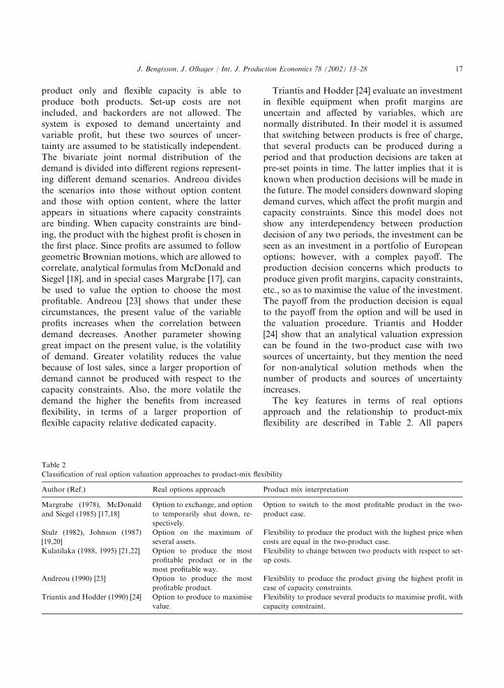
product only and flexible capacity is able toproduce both products. Set-up costs are notincluded, and backorders are not allowed. Thesystem is exposed to demand uncertainty andvariable profit, but these two sources of uncer-tainty are assumed to be statistically independent.The bivariate joint normal distribution of thedemand is divided into different regions represent-ing different demand scenarios. Andreou dividesthe scenarios into those without option contentand those with option content, where the latterappears in situations where capacity constraintsare binding. When capacity constraints are bind-ing, the product with the highest profit is chosen inthe first place. Since profits are assumed to followgeometric Brownian motions, which are allowed tocorrelate, analytical formulas from McDonald andSiegel [18], and in special cases Margrabe [17], canbe used to value the option to choose the mostprofitable. Andreou [23] shows that under thesecircumstances, the present value of the variableprofits increases when the correlation betweendemand decreases. Another parameter showinggreat impact on the present value, is the volatilityof demand. Greater volatility reduces the valuebecause of lost sales, since a larger proportion ofdemand cannot be produced with respect to thecapacity constraints. Also, the more volatile thedemand the higher the benefits from increasedflexibility, in terms of a larger proportion offlexible capacity relative dedicated capacity.

Triantis and Hodder [24] evaluate an investmentin flexible equipment when profit margins areuncertain and affected by variables, which arenormally distributed. In their model it is assumedthat switching between products is free of charge,that several products can be produced during aperiod and that production decisions are taken atpre-set points in time. The latter implies that it isknown when production decisions will be made inthe future. The model considers downward slopingdemand curves, which affect the profit margin andcapacity constraints. Since this model does notshow any interdependency between productiondecision of any two periods, the investment can beseen as an investment in a portfolio of Europeanoptions; however, with a complex payoff. Theproduction decision concerns which products toproduce given profit margins, capacity constraints,etc., so as to maximise the value of the investment.The payoff from the production decision is equalto the payoff from the option and will be used inthe valuation procedure. Triantis and Hodder[24] show that an analytical valuation expressioncan be found in the two-product case with twosources of uncertainty, but they mention the needfor non-analytical solution methods when thenumber of products and sources of uncertaintyincreases.The key features in terms of real options

approach and the relationship to product-mixflexibility are described in Table 2. All papers

Table 2

Classification of real option valuation approaches to product-mix flexibility

Author (Ref.) Real options approach Product mix interpretation

Margrabe (1978), McDonald

and Siegel (1985) [17,18]

Option to exchange, and option

to temporarily shut down, re-

spectively.

Option to switch to the most profitable product in the two-

product case.

Stulz (1982), Johnson (1987)

[19,20]

Option on the maximum of

several assets.

Flexibility to produce the product with the highest price when

costs are equal in the two-product case.

Kulatilaka (1988, 1995) [21,22] Option to produce the most

profitable product or in the

most profitable way.

Flexibility to change between two products with respect to set-

up costs.

Andreou (1990) [23] Option to produce the most

profitable product.

Flexibility to produce the product giving the highest profit in

case of capacity constraints.

Triantis and Hodder (1990) [24] Option to produce to maximise

value.

Flexibility to produce several products to maximise profit, with

capacity constraint.


above with the exception of Kulatilaka [21,22]assume processes of diffusion type to represent theevolution of the underlying asset. Kulatilaka[21,22] deals with processes of mean-reversiontype.Typically, only two products are considered,

which should not be representative to most of thesituations faced by producing companies. Triantisand Hodder [24] allow for multiple products intheir basic model, but are restricted to the two-product case in order to arrive at an analyticsolution. Therefore, to draw relevant conclusionsfrom a practical point of view more productswould need to be included in the valuationformula. The models of the production system inthe literature are also rather simple and show smallsimilarities to real manufacturing systems. Itshould therefore be of interest to include typicalfeatures of a real production situation, productiondecisions and the case of several products in avaluation of a product-mix flexible manufacturingsystem. Also, capacity constraints are only in-cluded in Andreou [23] and Triantis and Hodder[24], and set-up costs (or ‘‘switching’’ costs) areonly treated by Kulatilaka [21,22]. Thus, thecombination of capacity and set-up costs has notbeen treated previously. In real manufacturingsituation, product-mix flexibility would be re-stricted by both these factors. Therefore, in orderto capture the characteristics of the real case, forwhich our model is developed, we need toincorporate multiple products, set-up costs andcapacity constraints. Adding the fact that we areusing real data, we hope to contribute to the areaof real options valuation of product-mix flexibilityin particular, but also to the understanding of realoptions valuation of flexibility in general.

4. Option valuation

In this paper, as well as in some other realoption papers, the value of product-mix flexibilitydepends on the value of several underlyingvariables and can thereby be seen as a derivative.The value of a derivative can in some case beexpressed as analytical formulas, see, e.g., theBlack–Scholes formula [15], but often numerical

methods are required to estimate a value. In thispaper, as will be described in the next section, theoptions have a complex payoff pattern and aredependent on several underlying assets, and thisimplies that a numerical approach has to be used.The numerical approaches can be divided into

two groups. The first includes the lattice ap-proaches, see, e.g., Cox et al. [25] and Boyle et al.[26], and explicit and implicit finite differenceapproach, see, e.g., Brennan and Schwartz [27].The second includes the Monte Carlo approach,see, e.g., Boyle [28], dealing with one underlyingasset. A general disadvantage of the first group isan increasing degree of complexity when thenumber of underlying assets increases. In thisrespect the Monte Carlo approach offers an easierway to value options on several underlying asset.Another advantage of the Monte Carlo approachis that other types of processes than geometricBrownian motion, e.g., jump, jump-diffusion ormean-reverting processes, can be included rela-tively easily. However, two disadvantages are thatresults will lack accuracy due to significantstandard errors and it can be rather time consum-ing. This may call for error-reduction methods,which either reduce the required number ofsimulation runs with preserved standard error, orvice versa. Since Monte Carlo simulations may betime consuming it can be less suitable, e.g., in thecase of pricing financial assets. However, in thecase of valuing real options the time requiredshould be less critical.Since one of the objectives of this paper is to

evaluate flexibility in the case of several underlyingassets, it is important to use an approach whichsupports this and which makes it rather easy toadd or subtract an underlying asset. Based on theadvantages and disadvantages of each group, theMonte Carlo approach seems to be the mostappropriate in our case.Before running a Monte Carlo simulation, the

process subject to simulation has to be defined.First, we assume the case of a derivative dependenton a traded underlying asset S, whose dynamicsare given by the following geometric Brownianmotion:

dS ¼ aSdtþ sSdW ; ð1Þ


where a and s are the drift rate and volatility,respectively. The term dW represents the incre-ment of a Wiener process, which has a Gaussiandistribution with mean equal to zero and avariance equal to dt. We also assume that thereis a risk-free asset available, generating a non-stochastic risk-free rate of return, r. Using Ito’sformula, the dynamics of the two assets above andthe absence of arbitrage, the Black–Scholesequation [15] can be derived:

Ft þ rSFS þ 12s2S2FSS � rF ¼ 0; ð2Þ

FðT ; SÞ ¼ FðSÞ; ð3Þ

where Ft ¼ qF=qt etc. FðT ; SÞ denotes the term-inal boundary condition and is equal to the valueof the derivative at the exercise date T . Feynman–Kac’s stochastic representation formula gives asolution to the partial differential equation (PDE)in (2) and the value of the derivative F a time t,ðt5TÞ, which is given by

F t;Sð Þ ¼ e�rðT�tÞEQ½FðSðTÞÞ�; ð4Þ

where EQ½FðSðTÞÞ� represents the expected valueof the derivatives at exercise date, T , under the Q-measure and where the dynamics of S under Q arerepresented by

dS ¼ rSdtþ sSdW : ð5Þ

This implies that the option is valued using so-called risk neutral valuation, see, e.g., Cox andRoss [29]. Therefore, the derivative will not bevalued under the objective probabilities but valuedas if we were living in a risk neutral world. Thisdoes not mean that we in fact are risk neutral, orpretend to be, but that the option can be valuedregardless of the investors’ risk preferences. Theimplications relative the Monte Carlo approachand other approaches are that we have no use ofthe true drift a and the option can be valued bysimulating S using the risk-free rate, r. The s is,however, the same as in Eq. (1).In this paper the options are dependent on

several underlying variables, or more formallyexpressed, a vector process (D ¼ D1; :::;DN). TheBlack–Scholes equation, as well as Feynman–Kac’s stochastic representation formula, can bederived in the case of several underlying assets.

Thereby, derivatives on several underlying assetscan also be valued using risk neutral valuation.In this case the underlying assets are represented

by product demand or, expressed differently, byproduct demand revenues if prices are fixed. Sincedemand, or revenues, are non-traded assets, anumber of extensions and more or less restrictiveassumptions are required in order to make itpossible to use option pricing. This implies alsothat we cannot use the same line of reasoning asabove. However, one way to proceed is to use theapproach suggested by Constantinides [30]. To usethis approach assumptions regarding that marketsare complete and that there exist traded dynamicportfolios, which are perfectly correlated with thenon-traded real assets, have to be made. Accord-ing to Constantinides, any asset whether traded ornon-traded can be priced in a world withsystematic risk, e.g., using capital asset pricingmodel (CAPM), by replacing the actual drift witha certainty-equivalent by subtracting a risk-pre-mium. This approach is based on the intertempor-al CAPM by Merton [31] and is thereby dependenton assumptions such as that securities of firms aretraded on perfect capital markets, prices ofsecurities are log-normally distributed and inves-tors maximise their strictly concave and time-additive utility function. Thereby the PDE can bederived:

FtþXNi¼1

ðai � lmrimsiÞDiFi

þ1

2

XNi¼1

XNj¼1

rijsisjDiDjFij � rF ¼ 0;

lm ¼ðam � rÞ

sm; ð6Þ

lm is called the market price of risk and is definedas the excess total return of the market portfolioabove the risk-free rate of return per unit of risk;rij is the correlation between the demand ofproduct i and product j. ai is the growth rate ofthe non-traded underlying asset. If the underlyingasset is not traded, its growth rate may fall belowthe equilibrium total expected rate of return froman equivalent-risk traded financial security, see


McDonald and Siegel [18]. The rate-of-returnshortfall between the equilibrium rate and theactual rate is similar to a constant dividend yield.This leads to that the following PDE determinesthe value of the option:

Ft þXNi¼1

ðr� diÞDiFi

þ1

2

XNi¼1

XNj¼1

rijsisjDiDjFij � rF ¼ 0: ð7Þ

The Q-dynamics of the process Di is then given by

dDi ¼ r� dið ÞDidtþDi

PNj¼1 sijdWj ;

dWidWj ¼ 0; 8i; j i 6 ¼ j:ð8Þ

This is the type of process that will be used in theMonte Carlo simulation.

5. A real options model for product-mix flexibility

Here, we present a model using real options forthe valuation of product-mix flexibility that laterwill be applied to a real manufacturing system. Inan attempt to estimate the value of product-mixflexibility, the pay-off from the options of theflexible manufacturing system has to be defined.Before this can be done, a number of assumptionshave to be made concerning how productiondecisions are made. The following assumptions,regarding the options and the pay-off, are made:

(i) Production decisions are taken at pre-setpoints in time Tk, k 2 [1,K] andT15T25 � � �5TK . The time between anytwo pre-set points in time is allowed to vary.

(ii) If the value of the demand of producti; i 2 [1,N], does not exceed any set-up cost,SCil , of assembly line l; l 2 [1,L], no produc-tion of product i will take place.

(iii) If total demand is higher than actual totalcapacity, a selection between products takesplace with the objective to combine productsand assembly lines so as to maximise profits.

(iv) If production is constrained to produce thetotal demand of product i, Dik, due to capacitylimitations but is able to produce the quantityQilk such that the value of the produced

quantity exceeds set-up costs, then the productis a candidate for production.

(v) The price of product i is stable and exogen-ously given. Variable, fixed, and set-up costsare also stable but they may differ betweenassembly lines.

(vi) No inventory is considered.(vii)Demand that cannot be satisfied is considered

as lost sales. Thus, back-orders are notallowed.

These assumptions imply the following Eq. (9),which models the options and the pay-off of anoptimal production decision at time Tk:

Vk Tkð Þ ¼ Max

�XLl¼1

XNi¼1

Max½ðPi � VCilÞ:Qilk � SCil ; 0��

s:t

XLl¼1

Qilk4Dik

XNi¼1

Qilk4Clmax; ð9Þ

where Pi is the price of product i, VCil is thevariable cost of product i produced on line l, SCil

is the set-up cost for product i on line l, Clmax is the

maximum capacity of line l.Based on Eq. (9), a production system can be

regarded as a portfolio of European options toproduce since there are no interdependenciesbetween options in different periods. Investing ina system will give us numerous options to produceso as to maximise contribution margin, but tomake a correct investment decision, investmentand fixed costs must be considered. It should benoted that set-ups are considered as set-up costswhereas set-up times are not included explicitly.To estimate the value of the option with exercise

date Tk, the following procedure is carried out:

(i) Simulate ‘‘risk-free’’ demand, under the Q-measure, for all products i giving a demandvector D.

(ii) For a given D, optimise production so as tomaximise the value of the production sche-dule.

(iii) Perform the steps above n number of times.


(iv) Estimate the expected value of the option, i.e.,the mean of the payoff over all simulationruns.

(v) Discount the expected value with the risk-freerate to get the present value of the option.

This procedure is repeated to all availableoptions and an aggregate value of all options canthereafter be determined.

6. Case study

In this section, we first describe the manufactur-ing system and its environment. We then describethe modelling methodology and assumptions,before presenting and analysing the results.

6.1. Description

The case company, ABB Motors AB, producesmedium power electrical motors. The orderpenetration point is mixed between make-to-stock(MTS; 70% of total product volume) and make-to-order (MTO; 30%), the latter yielding higherprofit margins. MTO motors have a four-weekcustomer lead-time while MTS motors are shippedwithin 24 hours. The total order of a customer maybe large but is a mix of products. Individualproducts may differ substantially from a produc-tion point of view. The assembly operations atABB Motors are performed at three lines. Eachline is dedicated to a specific family of motors andeach family consists of several motors.The assembly line under study produces six

motors, which are divided into two groups, here

denoted by S (smaller) and B (bigger). Bothgroups are available with three different numbersof poles: 2, 4, and 6. Table 3 presents the averageweekly demand and the variable cost for eachmotor (these numbers are scaled since real data areconfidential).In order to satisfy customer needs, every motor

can be customised, leading to many differentvariants. However, customisation is relatively easyto manage and the impact on the assembly lineoperations and efficiency is negligible, whencompared to changeovers between sizes andnumber of poles. Therefore, set-up times due tocustomisation can be disregarded. The mostimportant point along the assembly line understudy with respect to product-mix flexibility is thewiring station. The operation that determines themain characteristics of a motor is carried out here,and this station is also the bottleneck. Currently,this station consists of one automatic wiringmachine and three semiautomatic machines. Table4 provides some basic characteristics (numbers arescaled relative the real data).

Table 3

Variable cost for different models of motor S and B,

respectively

Motor Average weekly

demand

Variable cost

(SEK)

S-2 184 569

S-4 298 479

S-6 38 479

B-2 38 691

B-4 148 691

B-6 22 691

Table 4

Characteristics of an automatic and a semiautomatic machine, respectively

Automatic machine Semiautomatic machine

Capacity 16motors/h 4motors/h

Number of producing hours/day 15 h 15 h

Set-up time between sizes 1.5 h 0.5 h

Set-up time between number of poles 0.7 h 0.7 h

Variable machine cost 400 SEK/h 340 SEK/h

Variable labour cost 549 SEK/h 366 SEK/h


The key issues that the company wants toaddress in this study are: (i) the optimal config-uration with respect to the level of automation –how should the mix of automatic and semiauto-matic resources be composed? (ii) the optimalconfiguration of flexible and dedicated equip-ment – should resources be dedicated to specificproducts or not? and (iii) the value of extracapacity – extra capacity is expected to add roomfor flexibility – however, how much is this worth?Before these questions are answered, modellingissues and assumptions made are discussed in thenext section.

6.2. Modelling and assumptions

Since option pricing is dependent on thebehaviour of the underlying assets, we have tomake assumptions regarding the behaviour of theprocesses. We assume that demand follows geo-metric Brownian motion, i.e., the same kind ofprocess as in Eq. (1). This assumption implies thatdemand is continuously log-normally distributed.A feature of modelling demand as a geometricBrownian motion is that the process will nevertake on any negative values. Other features of thisprocess are that there is a positive probability ofinfinite demand and that demand will be zero foreternity if demand ever hits the zero-barrier.Although these processes may not explain the trueprocesses perfectly, we make the assumption thatthese are reasonable proxies. The real demanddata contained a minor seasonal effect, but it isrelatively small and therefore disregarded. Theanalysis will be carried out using a correlationbetween products equal to zero and a relativestandard deviation of 150%. A standard deviationof 150% may be considered as high whencompared to previous literature. However, theydo not deal with real industrial cases. The realstandard deviations for the products under studywere 150% or higher. Therefore, 150% was chosenin order to reflect reality and still be relatively closeto previous research.In order to carry out the valuation we assume

that the prices of the products are exogenouslygiven and stable. Together with the company wemade the assumption of a ‘‘reasonable’’ margin of

15%, which is added to the variable cost ofproducing in the semiautomatic (with highervariable cost). Since prices are the same regardlessof the resource on which the motor is produced,this will lead to a somewhat higher margin forthose motors produced on the automatic machine.This approach does not really capture the differ-ence in profit contribution margin between MTOand MTS motors, but will handle the fact that thecost of producing is different between the twomachines. Based on these data and assumptions,the profit contribution margins are given inTable 5.Except for the value of the parameters discussed

above, we also need the risk-free rate of return andthe difference between the rate of return of theunderlying asset and that of the replicating asset.The risk-free rate of return is set to 5% and therate of return difference, d, is assumed to be zerofor all cases. The latter implies that the drift ratesof the underlying assets are equal to the drift rates(determined by, e.g., CAPM) of the portfolios thatreplicate the underlying asset.The assembly line under study has the same

proportion of MTO/MTS products as the com-pany in general, i.e., 30% MTO and 70% MTS.The replenishment lead time of a MTS motor isapproximately one week. The assembly lead timefor MTO products is also approximately oneweek. Therefore, production decisions are as-sumed to be based on weekly demand. If weeklycapacity is not sufficient, an MTO order isconsidered lost. This can be interpreted such thatorders within a week are accepted to the assemblycapacity limit using available-to-promise logic.

Table 5

Contribution margins of each product for the automatic and

semiautomatic resources

Motor Automatic

(SEK)

Semiautomatic

(SEK)

S-2 229 112

S-4 216 98

S-6 216 98

B-2 247 130

B-4 247 130

B-6 247 130


Orders in excess of this level are not taken. ForMTS orders, it is assumed that these need to bereplenished within a week; otherwise stock-outswill occur. Consequently, MTO and MTS pro-ducts can be treated in the same way from amodelling perspective. All orders that cannot bemet by weekly capacity are thus considered as lostsales.Since this analysis focuses on flexibility and

issues regarding flexibility, where decisions aremade with the objective to maximise profits givenvariable costs, relative prices, available capacity,etc., investment and fix costs are excluded. Thisexclusion does not change the general analysis. If afull analysis regarding the net present values ofdifferent configurations is needed these costs caneasily be incorporated.

6.3. Results

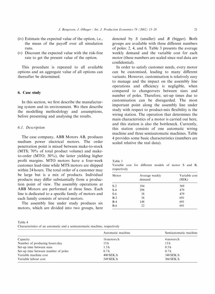
When carrying out the analysis we have lookedat production on a weekly basis. For each week,we have carried out 1000 ðn ¼ 1000Þ simulations toget the demand distribution. For every simulationrun the production is optimised, using AMPLsoftware, to find the maximum pay-off. From thepayoff distribution, we estimate the mean valueand discount it to get the present value of theoption.Fig. 1 shows the value of the option to produce

every week, from the first week until week 25 in asystem constituted of one automatic plus foursemiautomatic machines and with a capacity of1200 motors per week and 4300 motors per week,

respectively. This configuration was chosen as abase case, since it is very close to the actualresource mix of the company and it will allow forcomparisons between configurations having thesame level of capacity. The values of the options toproduce in Fig. 1 are very similar for differentweeks, although a slightly negative trend can beobserved.The negative trend could partly be explained by

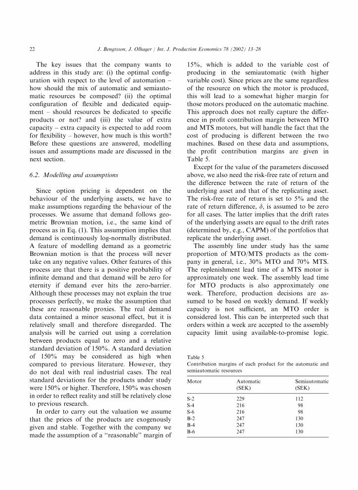
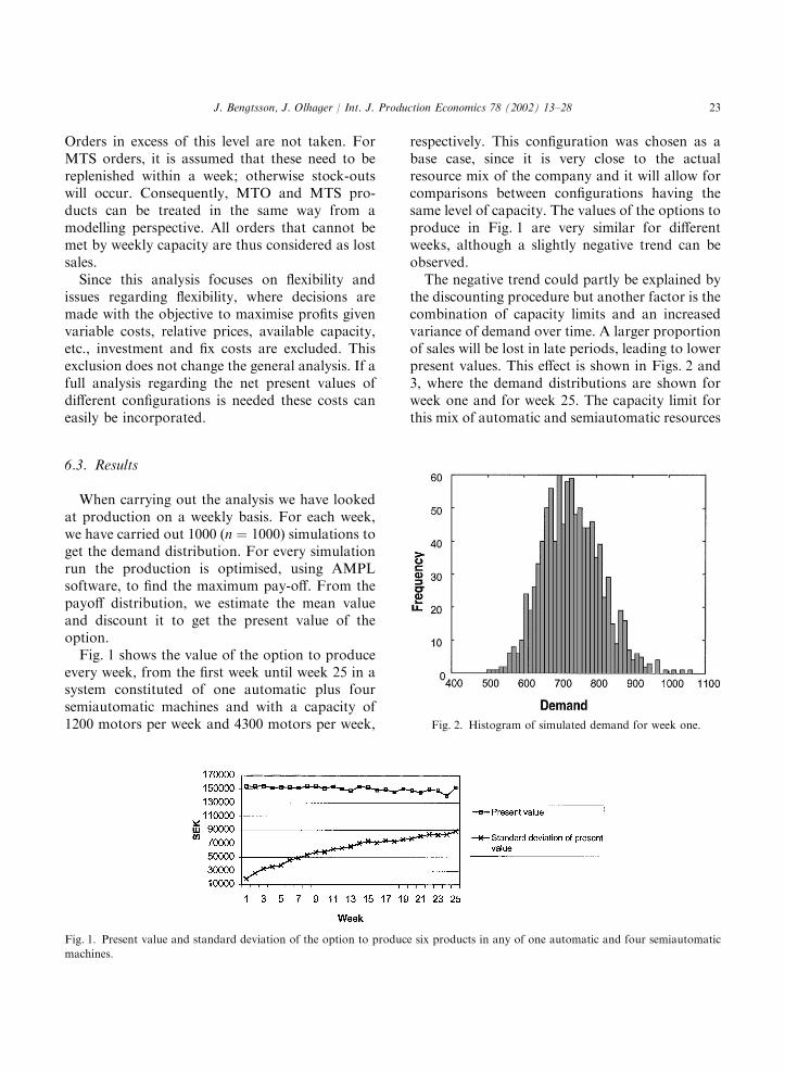
the discounting procedure but another factor is thecombination of capacity limits and an increasedvariance of demand over time. A larger proportionof sales will be lost in late periods, leading to lowerpresent values. This effect is shown in Figs. 2 and3, where the demand distributions are shown forweek one and for week 25. The capacity limit forthis mix of automatic and semiautomatic resources

Fig. 1. Present value and standard deviation of the option to produce six products in any of one automatic and four semiautomatic

machines.

Fig. 2. Histogram of simulated demand for week one.


is 2400 units per week. During week one, no lostsales are experienced, since the maximum demandover all simulation runs was lower than 1100, cf.,Fig. 2. However, the capacity limit becomes activequite a few times in week 25, which can be seen inFig. 3, leading to quite a few cases of lost sales.The capacity limit restricts the maximum payoff

to a certain amount. Simultaneously, the increasedvariance causes a heavier downward tail in thedistribution of total demand and consequently inthe distribution of total payoff. A heavier down-ward tail and a limited payoff upward result in aslightly decreasing mean value of the option thelonger the time to maturity. This effect was also

shown in a valuation of an option to produce inweek 50, which we performed, and where thepresent value was approximately 126 000 SEK andthe standard deviation approximately 103 000SEK.

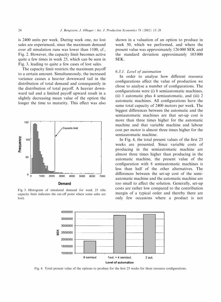
6.3.1. Level of automationIn order to analyse how different resource

configurations affect the value of production wechose to analyse a number of configurations. Theconfigurations were (i) 8 semiautomatic machines,(ii) 1 automatic plus 4 semiautomatic, and (iii) 2automatic machines. All configurations have thesame total capacity of 2400 motors per week. Thebiggest differences between the automatic and thesemiautomatic machines are that set-up cost ismore than three times higher for the automaticmachine and that variable machine and labourcost per motor is almost three times higher for thesemiautomatic machine.In Fig. 4, the total present values of the first 25

weeks are presented. Since variable costs ofproducing in the semiautomatic machine arealmost three times higher than producing in theautomatic machine, the present value of theconfiguration with 8 semiautomatic machines isless than half of the other alternatives. Thedifferences between the set-up cost of the semi-automatic machine and the automatic machine aretoo small to affect the solution. Generally, set-upcosts are rather low compared to the contributionmargin of a typical order and thereby there areonly few occasions where a product is not

Fig. 3. Histogram of simulated demand for week 25 (the

capacity limit indicates the cut-off point where some sales are

lost).

Fig. 4. Total present value of the options to produce for the first 25 weeks for three resource configurations.


produced due to the fact that the contributionmargin does not exceed the set-up cost. Thepresent values of the other two configurationsare almost the same. However, the configurationof two automatic machines has a slightly higherpresent value, which can be explained as follows.Since capacity utilisation is low on average, mostof the orders in both alternatives are produced onthe automatic resource, with a capacity of 1200motors a week and a higher profit margin. Theorders that cannot be produced on the automaticmachine have to be produced on either thesemiautomatic or automatic machines, respec-tively. Since these orders are rather few, thedifferences between these two configurations willbe rather low. If, for example, total demand waslarger, capacity limits were lower, or the varianceof demand was higher, the difference between thetwo would be larger.

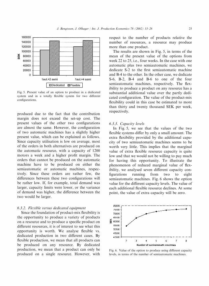
6.3.2. Flexible versus dedicated equipmentSince the foundation of product-mix flexibility is

the opportunity to produce a variety of productson a resource and to produce a specific product ondifferent resources, it is of interest to see what thisopportunity is worth. We analyse flexible vs.dedicated production in two different cases. Byflexible production, we mean that all products canbe produced on any resource. By dedicatedproduction, we mean that a product can only beproduced on a single resource. However, with

respect to the number of products relative thenumber of resources, a resource may producemore than one product.The results are shown in Fig. 5, in terms of the

mean of the present value of the options fromweek 22 to 25, i.e., four weeks. In the case with oneautomatic plus two semiautomatic machines, wededicate S-2 to the first semiautomatic machineand B-4 to the other. In the other case, we dedicateS-6, B-2, B-4 and B-6 to one of the foursemiautomatic machines, respectively. The flex-ibility to produce a product on any resource has asubstantial additional value over the partly dedi-cated configuration. The value of the product-mixflexibility could in this case be estimated to morethan thirty and twenty thousand SEK per week,respectively.

6.3.3. Capacity levelsIn Fig. 5, we see that the values of the two

flexible systems differ by only a small amount. Theextra flexibility provided by the additional capa-city of two semiautomatic machines seems to beworth very little. This implies that the marginalvalue of extra flexible resource capacity is quitelow and that we would not be willing to pay muchfor having this opportunity. To illustrate thephenomenon of reduced marginal value of flex-ibility, we analysed seven different capacity con-figurations running from two to eightsemiautomatic machines. Fig. 6 shows the optionvalue for the different capacity levels. The value ofeach additional flexible resource declines. At somepoint, the value of extra capacity will be zero.

Fig. 6. Value of the option to produce using different capacity

levels, in terms of the number of semiautomatic machines.

Fig. 5. Present value of an option to produce in a dedicated

system and in a totally flexible system for two different

configurations.


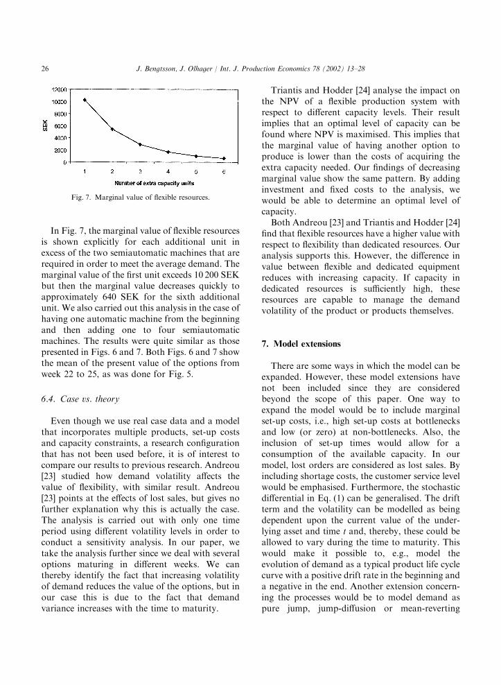
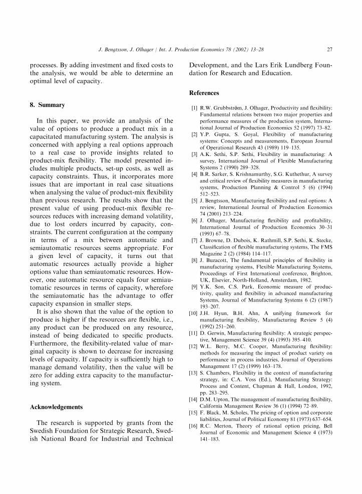
In Fig. 7, the marginal value of flexible resourcesis shown explicitly for each additional unit inexcess of the two semiautomatic machines that arerequired in order to meet the average demand. Themarginal value of the first unit exceeds 10 200 SEKbut then the marginal value decreases quickly toapproximately 640 SEK for the sixth additionalunit. We also carried out this analysis in the case ofhaving one automatic machine from the beginningand then adding one to four semiautomaticmachines. The results were quite similar as thosepresented in Figs. 6 and 7. Both Figs. 6 and 7 showthe mean of the present value of the options fromweek 22 to 25, as was done for Fig. 5.

6.4. Case vs. theory

Even though we use real case data and a modelthat incorporates multiple products, set-up costsand capacity constraints, a research configurationthat has not been used before, it is of interest tocompare our results to previous research. Andreou[23] studied how demand volatility affects thevalue of flexibility, with similar result. Andreou[23] points at the effects of lost sales, but gives nofurther explanation why this is actually the case.The analysis is carried out with only one timeperiod using different volatility levels in order toconduct a sensitivity analysis. In our paper, wetake the analysis further since we deal with severaloptions maturing in different weeks. We canthereby identify the fact that increasing volatilityof demand reduces the value of the options, but inour case this is due to the fact that demandvariance increases with the time to maturity.

Triantis and Hodder [24] analyse the impact onthe NPV of a flexible production system withrespect to different capacity levels. Their resultimplies that an optimal level of capacity can befound where NPV is maximised. This implies thatthe marginal value of having another option toproduce is lower than the costs of acquiring theextra capacity needed. Our findings of decreasingmarginal value show the same pattern. By addinginvestment and fixed costs to the analysis, wewould be able to determine an optimal level ofcapacity.Both Andreou [23] and Triantis and Hodder [24]

find that flexible resources have a higher value withrespect to flexibility than dedicated resources. Ouranalysis supports this. However, the difference invalue between flexible and dedicated equipmentreduces with increasing capacity. If capacity indedicated resources is sufficiently high, theseresources are capable to manage the demandvolatility of the product or products themselves.

7. Model extensions

There are some ways in which the model can beexpanded. However, these model extensions havenot been included since they are consideredbeyond the scope of this paper. One way toexpand the model would be to include marginalset-up costs, i.e., high set-up costs at bottlenecksand low (or zero) at non-bottlenecks. Also, theinclusion of set-up times would allow for aconsumption of the available capacity. In ourmodel, lost orders are considered as lost sales. Byincluding shortage costs, the customer service levelwould be emphasised. Furthermore, the stochasticdifferential in Eq. (1) can be generalised. The driftterm and the volatility can be modelled as beingdependent upon the current value of the under-lying asset and time t and, thereby, these could beallowed to vary during the time to maturity. Thiswould make it possible to, e.g., model theevolution of demand as a typical product life cyclecurve with a positive drift rate in the beginning anda negative in the end. Another extension concern-ing the processes would be to model demand aspure jump, jump-diffusion or mean-reverting

Fig. 7. Marginal value of flexible resources.


processes. By adding investment and fixed costs tothe analysis, we would be able to determine anoptimal level of capacity.

8. Summary

In this paper, we provide an analysis of thevalue of options to produce a product mix in acapacitated manufacturing system. The analysis isconcerned with applying a real options approachto a real case to provide insights related toproduct-mix flexibility. The model presented in-cludes multiple products, set-up costs, as well ascapacity constraints. Thus, it incorporates moreissues that are important in real case situationswhen analysing the value of product-mix flexibilitythan previous research. The results show that thepresent value of using product-mix flexible re-sources reduces with increasing demand volatility,due to lost orders incurred by capacity, con-straints. The current configuration at the companyin terms of a mix between automatic andsemiautomatic resources seems appropriate. Fora given level of capacity, it turns out thatautomatic resources actually provide a higheroptions value than semiautomatic resources. How-ever, one automatic resource equals four semiau-tomatic resources in terms of capacity, whereforethe semiautomatic has the advantage to offercapacity expansion in smaller steps.It is also shown that the value of the option to

produce is higher if the resources are flexible, i.e.,any product can be produced on any resource,instead of being dedicated to specific products.Furthermore, the flexibility-related value of mar-ginal capacity is shown to decrease for increasinglevels of capacity. If capacity is sufficiently high tomanage demand volatility, then the value will bezero for adding extra capacity to the manufactur-ing system.

Acknowledgements

The research is supported by grants from theSwedish Foundation for Strategic Research, Swed-ish National Board for Industrial and Technical

Development, and the Lars Erik Lundberg Foun-dation for Research and Education.

References

[1] R.W. Grubbstr.oom, J. Olhager, Productivity and flexibility:

Fundamental relations between two major properties and

performance measures of the production system, Interna-

tional Journal of Production Economics 52 (1997) 73–82.

[2] Y.P. Gupta, S. Goyal, Flexibility of manufacturing

systems: Concepts and measurements, European Journal

of Operational Research 43 (1989) 119–135.

[3] A.K. Sethi, S.P. Sethi, Flexibility in manufacturing: A

survey, International Journal of Flexible Manufacturing

Systems 2 (1990) 289–328.

[4] B.R. Sarker, S. Krishnamurthy, S.G. Kuthethur, A survey

and critical review of flexibility measures in manufacturing

systems, Production Planning & Control 5 (6) (1994)

512–523.

[5] J. Bengtsson, Manufacturing flexibility and real options: A

review, International Journal of Production Economics

74 (2001) 213–224.

[6] J. Olhager, Manufacturing flexibility and profitability,

International Journal of Production Economics 30–31

(1993) 67–78.

[7] J. Browne, D. Dubois, K. Rathmill, S.P. Sethi, K. Stecke,

Classification of flexible manufacturing systems, The FMS

Magazine 2 (2) (1984) 114–117.

[8] J. Buzacott, The fundamental principles of flexibility in

manufacturing systems, Flexible Manufacturing Systems,

Proceedings of First International conference, Brighton,

UK, Elsevier, North-Holland, Amsterdam, 1982.

[9] Y.K. Son, C.S. Park, Economic measure of produc-

tivity, quality and flexibility in advanced manufacturing

Systems, Journal of Manufacturing Systems 6 (2) (1987)

193–207.

[10] J.H. Hyun, B.H. Ahn, A unifying framework for

manufacturing flexibility, Manufacturing Review 5 (4)

(1992) 251–260.

[11] D. Gerwin, Manufacturing flexibility: A strategic perspec-

tive, Management Science 39 (4) (1993) 395–410.

[12] W.L. Berry, M.C. Cooper, Manufacturing flexibility:

methods for measuring the impact of product variety on

performance in process industries, Journal of Operations

Management 17 (2) (1999) 163–178.

[13] S. Chambers, Flexibility in the context of manufacturing

strategy, in: C.A. Voss (Ed.), Manufacturing Strategy:

Process and Content, Chapman & Hall, London, 1992,

pp. 283–295.

[14] D.M. Upton, The management of manufacturing flexibility,

California Management Review 36 (1) (1994) 72–89.

[15] F. Black, M. Scholes, The pricing of option and corporate

liabilities, Journal of Political Economy 81 (1973) 637–654.

[16] R.C. Merton, Theory of rational option pricing, Bell

Journal of Economic and Management Science 4 (1973)

141–183.


[17] W. Margrabe, The value of an option to exchange one asset

for another, Journal of Finance 33 (1) (1978) 177–186.

[18] R. McDonald, D. Siegel, Investment and the valuation of

firms when there is an option to shut down, International

Economic Review 26 (2) (1985) 331–349.

[19] R.M. Stulz, Options on the minimum or maximum of two

risky assets: Analysis and application, Journal of Financial

Economics 10 (2) (1982) 161–185.

[20] H. Johnson, Options on the maximum or the minimum of

several assets, Journal of Financial and Quantitative

Analysis 22 (3) (1987) 277–283.

[21] N. Kulatilaka, Valuing the flexibility of flexible manufac-

turing system, IEEE Transaction on Engineering Manage-

ment 35 (4) (1988) 250–257.

[22] N. Kulatilaka, The value of flexibility: A general model of

real options, in: L. Trigeorgis (Ed.), Real Options in

Capital Investment: Models, Strategies, and Application,

Praeger, New York, 1995.

[23] S.A. Andreou, A capital budgeting model for product-mix

flexibility, Journal of Manufacturing and Operations

Management 3 (1990) 5–23.

[24] A. Triantis, J. Hodder, Valuing flexibility as a complex

option, The Journal of Finance 45 (2) (1990) 549–565.

[25] J.C. Cox, S.A. Ross, M. Rubinstein, Option pricing: A

simplified approach, Journal of Financial Economics 7 (3)

(1979) 229–264.

[26] P.P. Boyle, J. Evnine, S. Gibbs, Numerical evaluation of

multivariate contingent claim, The Review of Financial

Studies 2 (1989) 241–250.

[27] M.J. Brennan, E.S. Schwartz, Finite difference methods

and jump processing arising in the pricing of contingent

claims: A synthesis, Journal of Financial and Quantitative

Analysis 13 (3) (1978) 461–474.

[28] P.P. Boyle, Options: A Monte Carlo approach, Journal of

Financial Economics 4 (1977) 323–338.

[29] J.C. Cox, S.A. Ross, The valuation of options for

alternative stochastic processes, Journal of Financial

Economics 3 (1976) 145–179.

[30] G.M. Constantinides, Market risk adjustment in project

valuation, The Journal of Finance 33 (2) (1978) 603–616.

[31] R.C. Merton, An intertemporal capital asset pricing

model, Econometrica 41 (1973) 867–887.


Documents

Valuation of product-mix flexibility using real options